Flow Measurement - Denver, Colorado · Flow Measurement Dr. James C.Y. Guo, ... Ci vil Engineering, U. of Colorado Denver ... 1.50 21.75 19.00 4.60 0.33 1.83 0.76

1

Flow Measurement

Dr. James C.Y. Guo, P.E., Professor and Director Civil Engineering, U. of Colorado Denver

Pitot-Static Tube

2

Pitot-tube for Velocity Measurement

Dr. James C.Y. Guo, Professor and P.E., Civil Engineering, U. of Colorado Denver

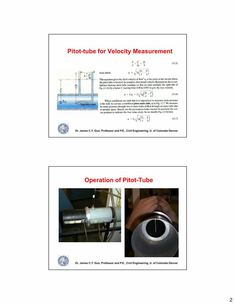
Operation of Pitot-Tube


3

Manometer and Pressure Differential

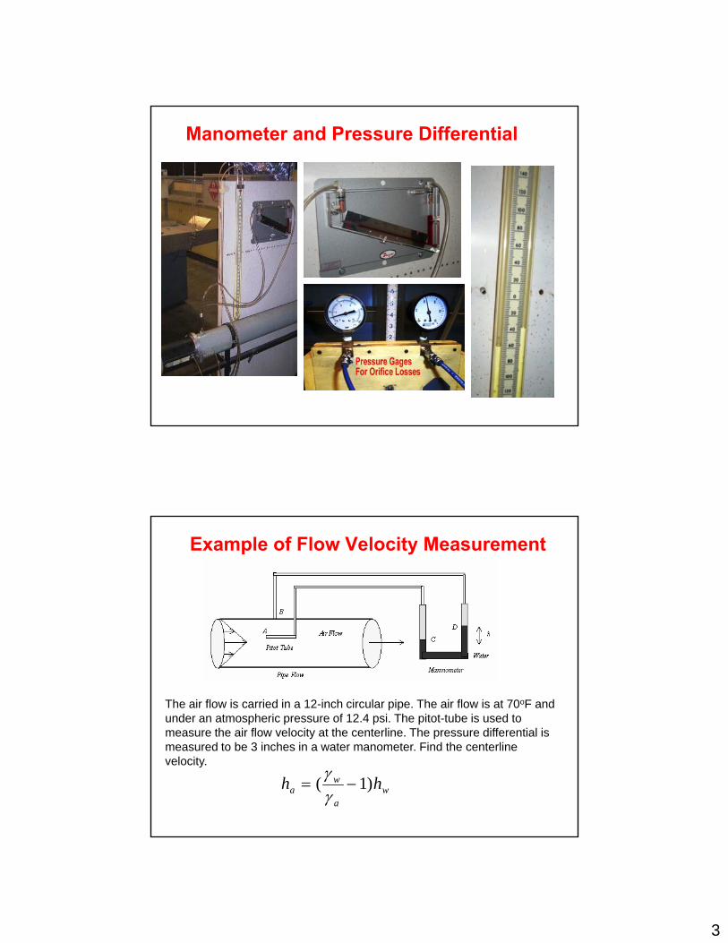
Example of Flow Velocity Measurement

The air flow is carried in a 12-inch circular pipe. The air flow is at 70oF and under an atmospheric pressure of 12.4 psi. The pitot-tube is used to

th i fl l it t th t li Th diff ti l imeasure the air flow velocity at the centerline. The pressure differential is measured to be 3 inches in a water manometer. Find the centerline velocity.

wa

wa hh )1( −=

γγ

4

Measurement of Flow Rate

0velocity in feet/sec

20

18

12

8

0 2 4 6 10 ftRadius


Example of Air Flow Velocity ContoursLocation Measured Average Circle Ring Incremental Accum

from Air Flow Flow Area Area Flow FlowPipe Cntr Velocity Velocity

cm mps mps sq m sq m mps mps58 0.000 1.06

0.875 0.107 0.093 0.09355 1 750 0 9555 1.750 0.95

1.885 0.133 0.251 0.34451 2.020 0.82

2.145 0.236 0.507 0.85143 2.270 0.58

2.315 0.127 0.295 1.14638 2.360 0.45

2.485 0.352 0.874 2.02018 2.610 0.10

2.670 0.102 0.272 2.2920 2 730 0 00

Calculate the cross sectional average velocityCalculate the ratio of the center velocity to average velocity

0 2.730 0.00

5

Review of Turbulent Flow Velocity Profile

rRRuU

rRRuUu mm −

−=−

−= log76.5ln5.2 ** (22)

Eq 22 has two unknown: Um and u*.

VfVU m 2.1)326.11( ≈+= (23)

8*fVu ==

ρτ (24)

6

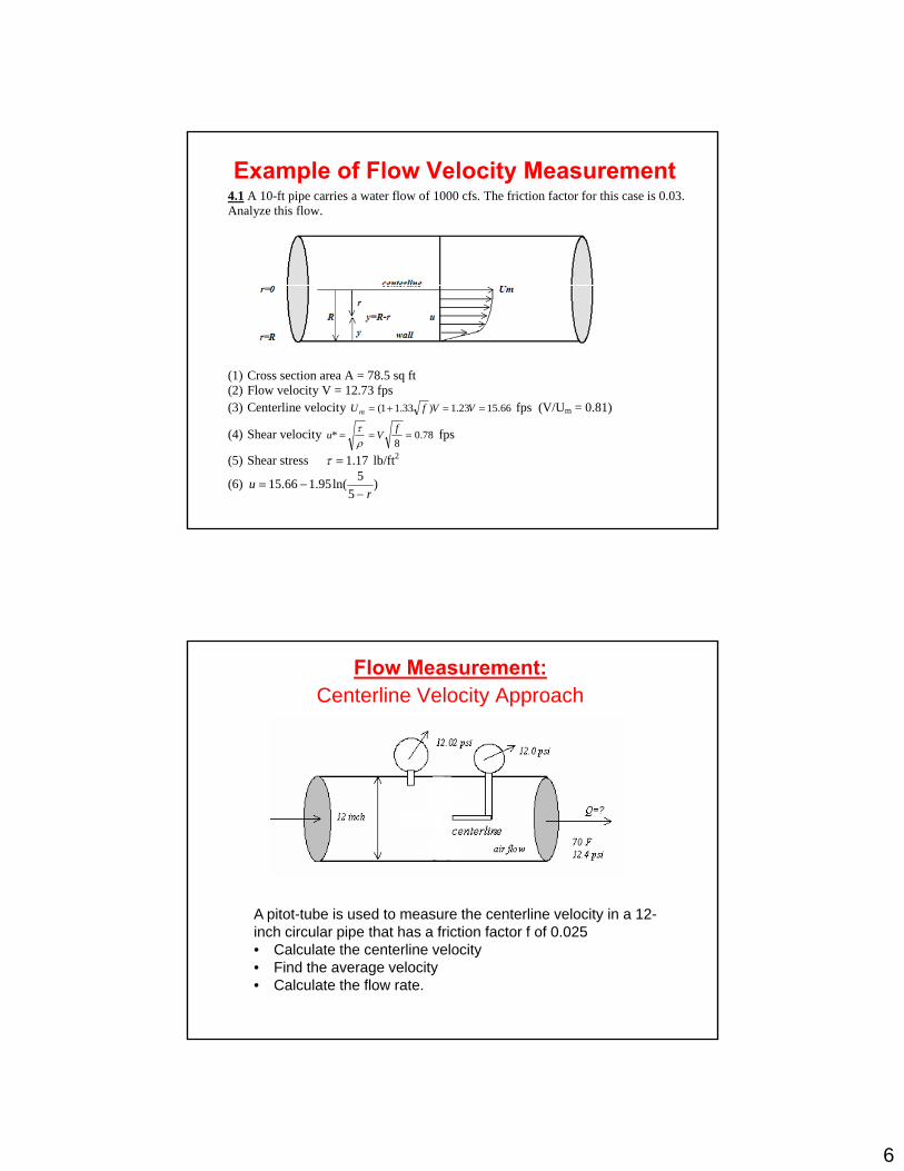
Example of Flow Velocity Measurement4.1 A 10-ft pipe carries a water flow of 1000 cfs. The friction factor for this case is 0.03. Analyze this flow.

(1) Cross section area A = 78.5 sq ft (2) Flow velocity V = 12.73 fps( ) y p(3) Centerline velocity 66.1523.1)33.11( ==+= VVfUm fps (V/Um = 0.81)

(4) Shear velocity 78.08

* ===fVu

ρτ fps

(5) Shear stress 17.1=τ lb/ft2

(6) )5

5ln(95.166.15r

u−

−=

Flow Measurement: Centerline Velocity Approach

A pitot-tube is used to measure the centerline velocity in a 12-inch circular pipe that has a friction factor f of 0.025• Calculate the centerline velocity• Find the average velocity• Calculate the flow rate.

7

Venturi Meter

iiii ghAVAQ == 2

i

a

ia

iiii

QQK

ghKAQ

ghVQ

=

= 2

Orifice Meter

ia

iiii

ghKAQ

ghAVAQ

=

==

2

2

Q

i

a

QQK =

Qi

Qa

8

Orifice OutletOrifice = an opening on a wallNozzle = a short converting pipe Jet = a high-speed stream of flow issued from a nozzle


9

Orifice Outlet Equation

c

i

cc

VC

AAC =

vc

iviccca

iiii

i

cv

CCKghKAghCACVAQ

ghAVAQ

VVC

=

===

==

=

22

2

)(2 oo YYgKAQ −=


Examples of Orifice Outlet


10

Weir Hydraulics


End Contraction

5.15.1)1.0(232 HLCHHnLgCQ ewd =−=

Cd=0.67


11

Examples of Orifice Outlet

An opening area in the flow field can be vertical, horizontal, or inclined. This opening area may be operated like an orifice when the entire opening area is submerged or operated like a weir if the opening area is partially submerged.

Q=min (Qweir, Qorifice) for a given depth


Example for Weir Flow

Find the release flow rate through the vertical orifice(1)when the water surface elevation at 5002 ft(2)when the water surface elevation at 5006 ft


12

Roadway Culvert

VNotch

13

Sluice Gate

gYACQ s 2= Cs=0.5 to 0.6


OPEN CHANNEL FLOW 1. Bottom Width B 2. Side Slope Z3. Top Width T= B + 2 Z Y4. Area A = 0.5 (T+B)Y5. Wetted Perimeter P = B + 2 Y(1+Z2)0.5

6. Hydraulic Radius R = A/P7. Hydraulic Depth D = A/T8. Froude Number Fr = U/(gD)0.5

14

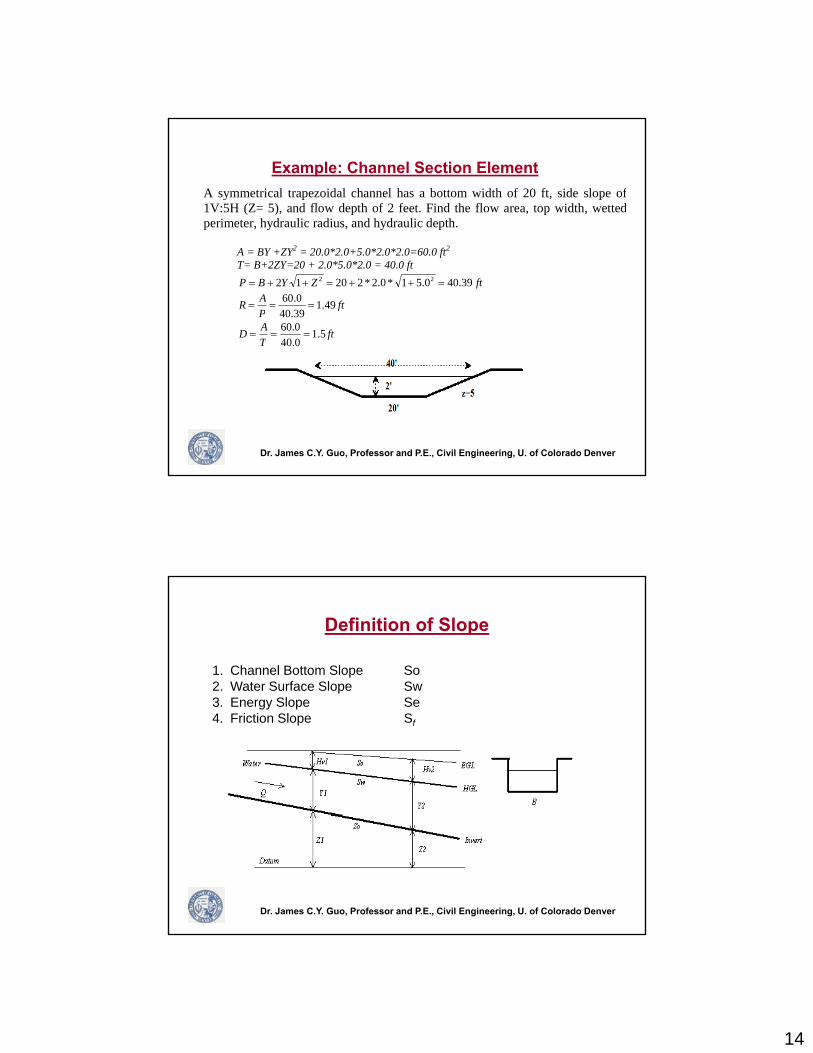
Example: Channel Section ElementA symmetrical trapezoidal channel has a bottom width of 20 ft, side slope of1V:5H (Z= 5), and flow depth of 2 feet. Find the flow area, top width, wettedperimeter, hydraulic radius, and hydraulic depth. A = BY +ZY2 = 20.0*2.0+5.0*2.0*2.0=60.0 ft2 T= B+2ZY=20 + 2.0*5.0*2.0 = 40.0 ft 39.400.51*0.2*22012 22 =++=++= ZYBP ft

49.139.400.60===

PAR ft

5.10.400.60===

TAD ft


Definition of Slope

1. Channel Bottom Slope So2. Water Surface Slope Sw3. Energy Slope Se4. Friction Slope Sf


15

Manning’s Eq is dimensionally inconsistent, but most widely accepted and used for channel design.K= 1.486 for feet-sec or K=1 for meter-sec.

Empirical Equations

SPAnKAS

PA

nKUAQ 3

235

21

32 −

=⎟⎠⎞

⎜⎝⎛==2

132

SRnKU =

Use the bottom slope to produce the normal depth (uniform flow)Use the energy slope to predict the flow depth (non-uniform flow)

Man-made Channels

Cross Waves

Super Elevation on Outer Bank

Uniform Flow

16

Prismatic Channel

Uniformity inAlignment StraightConstant Cross SectionConstant Channel SlopeConstant Channel RoughnessIt takes a long distance to develop uniform flow

Normal Flow1. Let Se=So to find Y=Yn2. Froude Number

A t id l h l i di h f 300 f Th h l h l fA trapezoidal channel carries a discharge of 300 cfs. The channel has a slope of0.005, roughness of 0.03, bottom width of 5 ft, and side slope of 1V:ZH, Z=2.0.Determine the normal depth. )25( nnn YYA +=

nnn YYP 47.40.52125 2 +=++=

005.0)47.45()]25([03.049.1 3/23/5 −++= nnn YYYQ

So e ha e Y 3 91 ft A 50 08 ft2 T 20 63 ft d U 5 99 fSo we have Yn= 3.91 ft, An=50.08 ft2, Tn=20.63 ft, and Un=5.99 fps. 43.2

63.2008.50

===TAD feet

68.043.22.32

99.5=

×=rF < 1.0. Subcritical flow!


17

Example of Weir and Channel Flow

Determine the flow from the weir measurementCalculate the normal flow condition downstream


Specific Energy=Y+U2/2g1. Illustration-- Sluice gate (ΔE=0)2. For a given Q, the curve for Y vs Es3. Flow regimes4 C iti l Fl4. Critical Flow 5. Increase or decrease of Q


18

Example for Specific Energy Curve

SPECIFIC ENERGY CURVE FOR TRAPEZOIDAL CHANNEL

Bottom Width B= 10.00 feetLeft Side Slope Z1= 3.00 ft/ftRight Side Slope Z2= 3.00 ft/ft

Design Flow Q= 100 cfsDesign Flow Q= 100 cfsBeginning Flow Depth Y= 0.50 ftIncremental Depth Dy= 0.25 ft

Flow Flow Top Flow Kinetic Sp. FroudeDepth Area Width Velocity Energy Energy Numer

Y A T u u^2/2g Es Fr ft sq ft ft fps ft ft

0.50 5.75 13.00 17.39 4.70 5.20 4.610.75 9.19 14.50 10.88 1.84 2.59 2.411.00 13.00 16.00 7.69 0.92 1.92 1.501.25 17.19 17.50 5.82 0.53 1.78 1.031.50 21.75 19.00 4.60 0.33 1.83 0.761.75 26.69 20.50 3.75 0.22 1.97 0.582.00 32.00 22.00 3.13 0.15 2.15 0.462 25 37 69 23 50 2 65 0 11 2 36 0 37

Specific Energy

2 00

2.50

3.00

3.50

4.00

4.50

5.00

w D

epth

in ft

2.25 37.69 23.50 2.65 0.11 2.36 0.372.50 43.75 25.00 2.29 0.08 2.58 0.302.75 50.19 26.50 1.99 0.06 2.81 0.263.00 57.00 28.00 1.75 0.05 3.05 0.223.25 64.19 29.50 1.56 0.04 3.29 0.193.50 71.75 31.00 1.39 0.03 3.53 0.163.75 79.69 32.50 1.25 0.02 3.77 0.144.00 88.00 34.00 1.14 0.02 4.02 0.124.25 96.69 35.50 1.03 0.02 4.27 0.114.50 105.75 37.00 0.95 0.01 4.51 0.10

0.00

0.50

1.00

1.50

2.00

0.00 1.00 2.00 3.00 4.00 5.00 6.00

Es in feet

Flow

Application of Energy Eq---Sluice Gate

Flow Flow Wetted Hy- Flow Flow Froude Sp Depth to SpDepth Area P-meter Radius Velocity rate Numer Energy Centroid Force

Y A P R U Q Fr Es Yh Fsft sq ft ft ft fps cfs ft ft klb10.00 500.0 92.5 5.41 9.30 4650.7 0.70 11.34 3.64 197.49

Flow Flow Top Flow Kinetic Sp. FroudeDepth Area Width Velocity Energy Energy Numer

Y A T u u^2/2g Es Fr ft sq ft ft fps ft ft

6.00 204.00 58.00 22.80 8.07 14.07 2.147.35 289.59 68.80 16.06 4.00 11.35 1.388.00 336.00 74.00 13.84 2.97 10.97 1.149.00 414.00 82.00 11.23 1.96 10.96 0.88

10.00 500.00 90.00 9.30 1.34 11.34 0.7011.00 594.00 98.00 7.83 0.95 11.95 0.5612.00 696.00 106.00 6.68 0.69 12.69 0.46


19

Critical Flow Fr=1.01. Froude number = 12. Critical flow depth 3. Critical Slope is solved by Manning’s eq with Yn=Yc4. Mild Slope and Steep Slope

012

== cTQF

1. Bottom Width B 2. Side Slope Z3. Top Width Tc= B + 2 Z Yc4. Area Ac = 0.5 (Tc+B)Yc5. Hydraulic Depth Dc = Ac/Tc6. Froude Number Fr = Uc/(gDc)0.5 =1.0

0.13 ==c

r gAF


cccccc

c SPAnKAS

PA

nKUAQ 3

2353

2−

=⎟⎟⎠

⎞⎜⎜⎝

⎛==

Example for Critical FlowGiven Design Information: Find Critical Slope

Bottom Width B= 5.00 feet Bottom Width B= 5.00 feetLeft Side Slope Z1= 3.00 ft/ft Left Side Slope Z1= 3.00 ft/ftRight Side Slope Z2= 3.00 ft/ft Right Side Slope Z2= 3.00 ft/ftManning's n N= 0.035 Manning's n N= 0.014Longitudinal Slope S= 0.0075 ft/ft Longitudinal Slope S= 0.00237 ft/ftDesign Flow Q= 500.00 cfs Design Flow Q= 500.00 cfs

Normal Flow ConditionNormal Flow Depth Yn= 4.27 feet Normal Flow Depth Yn= 3.68 feetWetted Periemeter P= 32.02 ft/ft Wetted Periemeter P= 28.27 ft/ftNormal Flow Area An= 76.12 sq ft Normal Flow Area An= 59.03 sq ftHydraulic Radius R= 2.38 feet Hydraulic Radius R= 2.09 feetFroude Number Fr= 0.73 Froude Number Fr= 1.01Difference In Q dQ= 0.00 ft/ft Difference In Q dQ= 0.00 ft/ft

Critical Flow Condition:Critical Depth Yc= 3.68 feetCritical Top Width Tc= 27.06 feetCritical Flow Area Ac= 58.93 sq ftFroude Number Fr= 1.01Froude Number Fr 1.01

0.13

2

==c

cr gA

TQF

cccccc

c SPAnKAS

PA

nKUAQ 3

2353

2−

=⎟⎟⎠

⎞⎜⎜⎝

⎛==

20

Specific Force 1. Illustration -- Jump (ΔF=0)2. For a given Q, the curve for Y vs Fs3. Flow regimes4. Critical Flow

Yo

4. Critical Flow 5. Increase or decrease of Q


Example for Specific Force Curve

SPECIFIC FORCE CURVE FOR TRAPEZOIDAL CHANNEL

Bottom Width B= 10.00 feetLeft Side Slope Z1= 3.00 ft/ftRight Side Slope Z2= 3.00 ft/ft

Design Flow Q= 100 cfs

Yo

Design Flow Q= 100 cfsBeginning Flow Depth Y 0.25 ftIncremental Depth Dy= 0.25 ft

Flow Flow Top Central Flow Sp. Froude SPDepth Area Width Depth Velocity Force Numer Energy

Y A T Yo u Fs Fr Esft sq ft ft ft fps Klbs ft

0.25 2.69 11.50 0.12 37.21 7.24 13.56 21.750.50 5.75 13.00 0.24 17.39 3.46 4.61 5.200.75 9.19 14.50 0.35 10.88 2.31 2.41 2.591.00 13.00 16.00 0.46 7.69 1.87 1.50 1.921.25 17.19 17.50 0.57 5.82 1.74 1.03 1.781.50 21.75 19.00 0.67 4.60 1.80 0.76 1.831.75 26.69 20.50 0.77 3.75 2.01 0.58 1.972 00 32 00 22 00 0 87 3 13 2 35 0 46 2 15

Specific Force

1.50

2.00

2.50

3.00

3.50

4.00

Flow

Dep

th in

ft

2.00 32.00 22.00 0.87 3.13 2.35 0.46 2.152.25 37.69 23.50 0.97 2.65 2.80 0.37 2.362.50 43.75 25.00 1.07 2.29 3.36 0.30 2.582.75 50.19 26.50 1.16 1.99 4.03 0.26 2.813.00 57.00 28.00 1.26 1.75 4.82 0.22 3.053.25 64.19 29.50 1.35 1.56 5.72 0.19 3.293.50 71.75 31.00 1.45 1.39 6.74 0.16 3.53

0.00

0.50

1.00

0.00 2.00 4.00 6.00 8.00

Fs in Klb

21

Application of Force Eq---Jump

Flow Flow Wetted Hy- Flow Flow Froude Sp Depth to SpDepth Area P-meter Radius Velocity rate Numer Energy Centroid Force

Y A P R U Q Fr Es Yh Fsft sq ft ft ft fps cfs ft ft klb

2.50 31.3 17.1 1.83 35.59 1112.1 4.35 22.11 1.17 79.06

Flow Flow Top Central Flow Sp. Froude SPDepth Area Width Depth Velocity Force Numer Energy

Y A T Yo u Fs Fr EsY A T Yo u Fs Fr Esft sq ft ft ft fps Klbs ft

2.50 31.25 15.00 1.17 35.59 79.05 4.34 22.175.00 75.00 20.00 2.22 14.83 42.37 1.35 8.41

10.00 200.00 30.00 4.15 5.56 63.79 0.38 10.4811.27 239.71 32.54 4.62 4.64 79.11 0.30 11.6012.00 264.00 34.00 4.89 4.21 89.60 0.27 12.28


Hydraulic Jump: from supercritical to subcritical flow

22

PUMP DESIGN

Pump

Pump Design by Dr. James Guo, UC-Denver

Pump = mechanic energy converted to fluid energyOutput energy = efficiency x Input energy

23

Pump Head and Units fp HHhH +=+ 21

A pump is identified by its rotating speed, power, and efficiency.

Horse Power η

γ550

pQhHp = for ft-second units where Hp in horse power = 550 lb-ft,

Kilowatts η

γ1000

pQhKw = for meter-second units. One Horse Power = 0.746 Kw

Pump Net Positive Suction Head

PumptoLossesHdSuctionHeaH i +=+Fi d S ti H d PumptoLossesHdSuctionHeaH pumpin ++

gVZ

PH pump

pumpvapor

pump 2

2++=

γ

inatm

in ZP

H +=γ

Find Suction Head.

24

Pump Net Required Discharge Head

PumpFromLossesHeHeadDischH +=+ argFi d Di h H d PumpFromLossesHeHeadDischH outpump +=+ arg

gVZ

PH pump

pumpvapor

pump 2

2++=

γ

Outatm

Out ZP

H +=γ

Find Discharge Head.

Design Pump Head and Horsepower

Find Pump Head

sOutflowLosInflowLossHhH outpin ++=+

Find the pump head with Q=2 cfsIs the pump head equal to suction head + discharge head?Why do we have to calculate suction and discharge heads?

d u p ead

25

Affinity Law

Pump Model and Prototype

1. Basic DataModel Pump Diameter D1 1.00 feet

Pump Rotational Speed n1 1800.00 rpmProto-type Pump Diameter D2 2.00 feet

P R t ti l S d 2 1200 00

Performance Curve (Model Pump)

4045

Pump Rotational Speed n2 1200.00 rpm

2. Pump Affiniity and Similarity Laws: Proto-type to Model RatiosRotational speed ratio n*=n2/n1 0.67 Diameter ratio D*=D2/D1 2.00Head ratio h*=h2/h1 1.78Flow ratio Q*=Q2/Q1 5.33 Power ratio P*=P2/P1 9.48

3. Pump Performance Curve Enter model pump curve:

Flowrate cfs 0.10 0.50 0.75 1.00 1.50 2.00 2.50

05

101520253035

0

0 1 2 3Flow rate in cfs

Pum

p he

ad in

feet

Pump Design by Dr. James Guo, UC-Denver

Pumphead feet 40.00 39.00 37.00 33.00 22.00 10.00 2.00

Calculate Proto-type pump curveFlowrate cfs 0.53 2.67 4.00 5.33 8.00 10.67 13.33Pumphead feet 71.11 69.33 65.78 58.67 39.11 17.78 3.56

26

Pump in series or in parallel

Calculate Proto-type pump curveFlowrate cfs 0.53 2.67 4.00 5.33 8.00 10.67 13.33Pumphead feet 71.11 69.33 65.78 58.67 39.11 17.78 3.56

3. Pump Performance Curve for multiple pumps Flowrate Number of Pump in Series Pumphead Number of Pump in Parallel

Q 1 2 3 4 Hp 1 2 3 4cfs Pump head in feet, Hp feet Flow rate in cfs, Q

0.53 71.11 142.22 213.33 284.44 71.11 0.53 1.07 1.60 2.132.67 69.33 138.67 208.00 277.33 69.33 2.67 5.33 8.00 10.674.00 65.78 131.56 197.33 263.11 65.78 4.00 8.00 12.00 16.005.33 58.67 117.33 176.00 234.67 58.67 5.33 10.67 16.00 21.338.00 39.11 78.22 117.33 156.44 39.11 8.00 16.00 24.00 32.00

10.67 17.78 35.56 53.33 71.11 17.78 10.67 21.33 32.00 42.6713.33 3.56 7.11 10.67 14.22 3.56 13.33 26.67 40.00 53.33

A and Q

Documents

Flow Measurement - Denver, Colorado · Flow Measurement Dr. James C.Y. Guo, ... Ci vil Engineering, U. of Colorado Denver ... 1.50 21.75 19.00 4.60 0.33 1.83 0.76