Embed Size (px)
Citation preview

Flow instabilities in centrifugal compressors atlow mass flow rate
by
Elias Sundstrom
December 2017
Technical Reports
Royal Institute of Technology
Department of Mechanics
SE-100 44 Stockholm, Sweden

Akademisk avhandling som med tillstand av Kungliga Tekniska Hogskolan iStockholm framlagges till offentlig granskning for avlaggande av teknologiedoktorsexamen onsdagen den 13 December 2017 kl 10:15 i sal D3, KungligaTekniska Hogskolan, Lindstedtsvagen 5, Stockholm.
TRITA-MEK Technical report 2017:12ISSN 0348-467XISRN KTH/MEK/TR-17/12-SEISBN 978-91-7729-555-6
c�Elias Sundstrom 2017
Universitetsservice US–AB, Stockholm 2017

To Ellinor, Sunniva and Jan, whose sacrifices made it possible.


Flow instabilities in centrifugal compressors at low massflow rate
Elias Sundstrom
The Competence Center for Gas Exchange (CCGEx), KTH Mechanics, RoyalInstitute of Technology, SE-100 44 Stockholm, Sweden
AbstractA centrifugal compressor is a mechanical machine with purpose to convert kineticenergy from a rotating impeller wheel into the fluid medium by compressingit. One application involves supplying boost air pressure to downsized internalcombustion engines (ICE). This allows, for a given combustion chamber volume,more oxygen to the combustion process, which is key for an elevated energeticefficiency and reducing emissions. However, the centrifugal compressor is limitedat off-design operating conditions by the inception of flow instabilities causingrotating stall and/or surge. These instabilities appear at low flow rates andtypically leads to large vibrations and stress levels. Such instabilities affectthe operating life-time of the machine and are associated with significant noiselevels.
The flow in centrifugal compressors is complex due to the presence of a widerange of temporal- and spatial-scales and flow instabilities. The success fromconverting basic technology into a working design depends on understandingthe flow instabilities at off-design operating conditions, which limit significantlythe performance of the compressor. Therefore, the thesis aims to elucidate theunderlying flow mechanisms leading to rotating stall and/or surge by means ofnumerical analysis. Such knowledge may allow improved centrifugal compressordesigns enabling them to operate more silent over a broader operating range.
Centrifugal compressors may have complex shapes with a rotating partthat generate turbulent flow separation, shear-layers and wakes. These flowfeatures must be assessed if one wants to understand the interactions among theflow structures at different locations within the compressor. For high fidelityprediction of the complex flow field, the Large Eddy Simulation (LES) approachis employed, which enables capturing relevant flow-driven instabilities underoff-design conditions. The LES solution sensitivity to the grid resolution usedand to the time-step employed has been assessed. Available experimentaldata in terms of compressor performance parameters, time-averaged velocity,pressure data (time-averaged and spectra) were used for validation purposes.LES produces a substantial amount of temporal and spatial flow data. Thisnecessitates efficient post-processing and introduction of statistical averagingin order to extract useful information from the instantaneous chaotic data. Inthe thesis, flow mode decomposition techniques and statistical methods, suchas Fourier spectra analysis, Dynamic Mode Decomposition (DMD), ProperOrthogonal Decomposition (POD) and two-point correlations, respectively, areemployed. These methods allow quantifying large coherent flow structures at
v

frequencies of interest. Among the main findings a dominant mode was foundassociated with surge, which is categorized as a filling and emptying processof the system as a whole. The computed LES data suggest that it is causedby substantial periodic oscillation of the impeller blade incidence flow angleleading to complete system flow reversal. The rotating stall flow mode occurringprior to surge and co-existing with it, was also captured. It shows rotating flowfeatures upstream of the impeller as well as in the diffuser.
Key words: Centrifugal Compressor, flow instabilities, rotational flows, rotat-ing stall, surge, compressible Large Eddy Simulation.
vi

Flodesinstabilitet i centrifugalkompressor vid lagt mass-flode
Elias Sundstrom
The Competence Center for Gas Exchange (CCGEx), KTH Mekanik, KungligaTekniska Hogskolan, SE-100 44 Stockholm, Sverige
SammanfattningEn centrifugalkompressor ar en mekanisk maskin dar syftet ar att omvand-la kinetisk energi fran ett roterande pumphjul genom komprimering av ettflodesmedium. En applikation innebar att oka lufttrycket i sma forbranningsmoto-rer (ICE). Detta medger, for en given volym i forbranningskammaren, mer syretill forbranningsprocessen, vilket ar en nyckel till en forhojd energieffektivitetoch minskning av utslapp. Centrifugalkompressorer ar emellertid begransadevid icke optimala driftsforhallanden p.g.a. flodesinstabiliteter som orsakar rote-rande stall och eller surge. Dessa instabiliteter uppstar vid laga floden och ledervanligen till stora vibrationer och stressnivaer. Sadana instabiliteter paverkarkompressorns operativa livstid och forknippas med signifikanta ljudnivaer.
Flodet i centrifugalkompressorer ar komplext pa grund av ett brett intervallav temporala och spatiala skalor samt flodesinstabiliteter. Formagan att konver-tera grundlaggande teknik till en fungerande design beror pa en forstaelse avflodesinstabiliter vid icke-optimala driftsforhallanden som begransar kompres-sorns prestanda. Ambitionen med avhandlingen ar att med hjalp av numeriskanalys belysa underliggande flodesmekanismer som leder till roterande stall ocheller surge. Sadan kunskap kan mojliggora forbattringar i centrifugalkompres-sorns konstruktion som gor att turboaggregat opererar tystare over ett bredarearbetsomrade.
Centrifugalkompressorer kan ha en komplex utformning med roterandedelar som genererar turbulenta flodesseparationer, skjuvskikt och vakar. Des-sa flodesfenomen bor utvarderas om man vill forsta interaktionerna mellanflodesstrukturer pa olika spatiala omraden i kompressorn. For hog noggrannhetvid uppskattning av komplexa flodesfalt anvands Large Eddy Simulation (LES).Denna metod mojliggor upplosning av relevanta flodesdrivna instabiliteten undericke-optimala betingelser. Resultatkansligheten med LES har underskots medavseende pa tathet i berakningsnatet samt i storleken pa tidssteget. Tillgangligexperimentell matdata avseende kompressorns prestandaparametrar, tidsme-delvarderade hastigheter och tryckdata (tidsmedelvarderade samt spektra) haranvants for valideringsandamal. LES producerar en betydande mangd temporaloch spatial data. Detta kraver en effektiv efterbehandling och tillampning avstatistisk medelvardering for att extrahera anvandbar information fran denmomentant kaotiska datamangden. I avhandlingen anvands olika dekomposi-tionstekniker och statistiska metoder, t.ex. Fourier spektralanalys, DynamicMode Decomposition (DMD), Proper Ortogonal Decomposition (POD) ochtvapunktskorrelation. Dessa metoder mojliggor kvantifiering av storskaliga och
vii

sammanhangande flodesstrukturer vid intressant frekvenser. Ett betydande re-sultat pavisar en dominerande flodesmod som ar identifierad som surge. Dennamod kan kategoriseras som en systemoscillation med periodisk fyllning ochtomning av systemet som helhet. Data fran LES tyder pa att den orsakas aven betydande periodisk variation av impellerbladens anblasningsvinkel, somorsakar fullstandig flodesomriktning i systemet. En flodesmod relaterad tillroterande stall kunde ocksa pavisas. Den ses forekomma innan eller samexisteramed surgefenomenet. Det kannetecknas av roterande virvelstrukturer uppstromsom pumphjulet men aven nedstroms i diffusorn.
Nyckelord: Centrifugalkompressor, flodesinstabiliter, roterande floden, rote-rande stall, surge, kompressibel Large Eddy Simulation.
viii

Preface
Flow instabilities at off-design operating conditions in centrifugal compressorsare examined in the thesis. The main focus is at low flow rates and exploring theonset mechanism of rotating stall and surge. The first part of the thesis providesan overview of centrifugal compressor terminology as wells as an introductionto preliminary aerodynamic design technology and analysis. This includes abrief description of reduced order modeling for fast assessment of compressorperformance maps together with linearized modeling for assessment of stabilitylimits. More advanced numerical simulation methodologies, i.e. steady-stateReynolds Averaged Navier-Stokes (RANS) and the Large Eddy Simulation (LES)approach, are also discussed. The second part of the thesis includes severalpapers, as listed further below. Papers 1, 3 and 5 are conference proceedingcontributions whereas Papers 2, 4 and 6 have been submitted for publication.All papers have been adapted to comply with the thesis format.
Paper 1. E. Sundstrom, B. Semlitsch & M. Mihaescu, 2014. Assessmentof the 3D Flow in a Centrifugal compressor using Steady-State and UnsteadyFlow Solvers. SAE Technical paper (2014-01-2856).
Paper 2. E. Sundstrom, B. Semlitsch & M. Mihaescu, 2017. GenerationMechanisms of Rotating Stall and Surge in Centrifugal Compressors. Acceptedfor publication in Flow, Turbulence and Combustion, Springer, 2017.
Paper 3. E. Sundstrom, B. Semlitsch & M. Mihaescu, 2015. CentrifugalCompressor: The Sound of Surge. AIAA Technical paper, AIAA 2015-2674,https://doi.org/10.2514/6.2015-2674.
Paper 4. E. Sundstrom, B. Semlitsch & M. Mihaescu, 2017. Acousticsignature of flow instabilities in radial compressors. Under review J. of Soundand Vibration.
Paper 5. E. Sundstrom, B. Kerres & M. Mihaescu, 2016. Evaluationof Centrifugal Compressor Performance Models using Large Eddy SimulationData. ASME Technical paper, GT2016-57169.
Paper 6. E. Sundstrom, M. Mihaescu, M. Giachi, E. Belardini & V.Michelassi, 2017. Analysis of vaneless diffuser stall instability in a centrifugalcompressor. Under review Int. J. Turbomach. Propuls. Power.
December 2017, Stockholm
Elias Sundstrom
ix


Contents
Abstract v
Sammanfattning vii
Preface ix
Nomenclature xiv
Part I - Overview, Outcomes and Discussions
Chapter 1. Introduction 1
1.1. Background and Motivation 2
1.2. Objectives and Research questions 4
Chapter 2. Theory of Centrifugal Compressors 10
2.1. Geometry and characteristics 10
2.2. 1D Compressor modeling theory 13
2.3. Flow features of stall, rotating stall and surge 19
2.4. Theoretical stability criteria 20
Chapter 3. Modeling Compressor Flow 29
3.1. Reynolds Averaged Navier-Stokes (RANS) 33
3.2. Curvature correction 35
3.3. Large Eddy Simulation (LES) 41
3.4. Advanced post-processing 43
3.5. Ffowcs Williams and Hawkings equation 47
Chapter 4. Numerical Methods 50
4.1. Discretization 50
Chapter 5. Results: Highlights and Discussion 55
xi

Chapter 6. Conclusions 74
6.1. Contributions 74
6.2. Proposal for future work 77
Chapter 7. Publications 80
Acknowledgements 83
Bibliography 84
xii

Part II - Papers
Paper 1. Assessment of the 3D Flow in a Centrifugal compressorusing Steady-State and Unsteady Flow Solvers 91
Paper 2. Generation Mechanisms of Rotating Stall and Surgein Centrifugal Compressors 117
Paper 3. Centrifugal Compressor: The Sound of Surge 137
Paper 4. Acoustic signature of flow instabilities in radialcompressors 163
Paper 5. Evaluation of Centrifugal Compressor PerformanceModels using Large Eddy Simulation Data 189
Paper 6. Analysis of vaneless diffuser stall instability in acentrifugal compressor 211
xiii

Nomenclature
m Mass flow rate [kg/s]h Specific enthalpy [J/kg]s Specific entropy [J/kg-K]c Speed of sound [m/s]f Frequency [Hz]k Wave number [1/m]L Characteristic length [m]Ma Mach number [-]p Pressure [Pa]r, θ, z Radial, Tangential and Axial coordinates, [m]x, y, z Cartesian coordinates, [m]η Isentropic efficiencyΦ Phase angle [radian]γ Ratio of specific heatβ angle [o]cp Specific heat at constant pressure [J/kg-K]t Time [s]T Temperature [Kelvin]�u Velocity vector [m/s]�U Mean velocity [m/s]ρ Density [kg/m3]ω Angular frequency [rad/s or 1/s]RO Rotating Order, Normalized angular velocityBPF Blade Passing FrequencyV Volume [m3]Re Reynolds numberk Turbulent kinetic energy [m2/s2]� Dissipation rate [m2/s3]
Subscript0 Total, ambient or mean variable1 upstream of the impeller2 downstream of the impellerref variable is referred to reference valueb blade
Superscript— Average∼ Favre average� Fluctuation
Only commonly used symbols and quantities are listed above. Other abbrevia-tions and quantities are explained in the text at first occurrence.
xiv

Part I
Overview, Outcomes andDiscussions

Chapter 1
Introduction
Since the 1950s there is a variety of scientific evidence showing global warming:a climate change due to observed century-scale rise of the Earth’s averagetemperature. Global warming is believed to have anticipated effects such asrising sea levels, expansions of deserts, reoccurring extreme weather events andocean acidification1. Such consequences will ultimately influence security offood supply due to decreasing crop yields and the survival of endangered species.
The human influence is concluded as the most likely cause, and one signifi-cant factor is vehicle emissions from cars and trucks on the open road. In theEuropean Union (EU) the majority (99%) of new registered cars and trucksrely on an internal combustion engine (ICE) as the main propulsion system2.Although in recent years, the market has seen a growing share of electrifiedpropulsion units. However, due to the mature technology with ICE it’s projectedto dominate the market for the foreseeable future. The problem is that themajority of ICE systems are based on combustion of fossil based fuels (e.g.Gasoline or Diesel), where the main combustion products are carbon dioxide(CO2) and water. CO2 is a greenhouse gas, which contributes to the globalwarming. Combustion of Gasoline or Diesel may also yield toxic byproductsthat are dangerous for humans and other organisms, e.g. carbon monoxide(CO), nitrogen oxides (NOx), hydrocarbons (HC) and particulate matter (PM).The type and amount of emissions depend strongly on the local conditions (suchas pressure, temperature and equivalence ratio) in the cylinder. Improvingthe fuel economy of ICE has a direct impact on reducing emissions, which ispositive for the environment. The European Union (EU) legislation regardingvehicle emissions has become more stringent in the past few decades, and fur-ther restrictions are expected to follow 3, 4, 5. By 2020 the objective dictates40% CO2 reduction for cars and light-duty vehicles and 30% for heavy-dutytrucks. Generated noise is another concern with combustion engines, whichhas a disturbing impact in densely populated residential areas. This is also
1https://climate.nasa.gov/evidence/2ACEA (2017). European automotive manufacturers’ association: Consolidated registrations.3Regulation (EU) No 333/2014 of the European Parliament and of the Council4https://ec.europa.eu/clima/policies/transport/vechiles/heavy/documentation.htm5http://www.iea.org/publications/freepublications/publication/
CO2EmissionsFromFuelCombustion2017Overview.pdf
1

2 1. Introduction
regulated within EU, as a maximum sound pressure level (SPL) due to vehicledrive-by on the open road6.
1.1. Background and Motivation
ICE can be described as a reacting flow system. It is a system containing amulti-component fluid mixture whose constituents react chemically with eachother. The mixture contains a substantial amount of chemical energy lockedwithin molecular bonds. Upon combustion the available chemical energy istransformed into thermal energy, which in turn is transformed, partially, intomechanical energy in the power-train of the vehicle, thus moving the vehicle.For an efficient combustion process there is a need to regulate the concentrationspecies present in the reaction. This is so since chemical reaction of fuels likehydrocarbons are composed of a large number of reaction steps with a wide rangeof time scales. In addition, turbulence imposes its own time- and length-scalesthat only partially overlap with the species time-scales. Resolving all time-and length-scales relevant to combustion is out of reach to current knowledgeand computational power. Without going into details of stoichiometric balanceequations between reactant and product species, respectively, it has beenidentified by other researchers that some few so called integral parameters areinfluential in defining the overall power output from ICE. The engine poweroutput can be modeled (in zero dimension) with an elementary equation asfollows, see e.g. Heywood (1988):
P =1
2· n · pme · VSW (1.1)
The engine power is thus seen to depend mainly on the engine speed n, thebrake mean effective pressure pme (an indication of the engine load) and theswept cylinder volume VSW . The last parameter is a measure of the enginesize. These parameters are included to yield different frictional losses. Forexample, the engine speed is associated with a quadratic increase in frictionloss. It is approximately constant with respect to the engine load, and increaseslinearly with engine size, see experimental works by Guzzella & Sciarretta(2007); Ben-Chaim et al. (2013); Leduc et al. (2003). Accordingly, reducingthe engine speed would theoretically have a positive effect on frictional losses.However, too low engine speeds may introduce side effects associated withnon-smooth operations causing high vibrational levels. The next candidateparameter for reduced frictional losses to consider is VSW , i.e. the engine size.This is one of the more promising engineering directions for improved fueleconomy and thus lowering the emission levels (e.g. CO2). Reduced engine sizeis commonly attributed to downsizing of the modern reciprocating combustionengine. Downsizing naturally leads to less thermal and frictional losses butlowers the power output. This is compensated by adding a well matchedturbocharging unit in gas exchange circuit, as sketched in Fig. 1.1. The aim isto convert some of the exhaust gas enthalpy into rotational kinetic energy of
6Directive 2002/49/EC relating to the assessment and management of environmental noise.

1.1. Background and Motivation 3
the turbine wheel, which otherwise is being wasted, c.f. Guzzella & Sciarretta(2007); Ben-Chaim et al. (2013); Leduc et al. (2003).
The turbine wheel is spooled to high rotational speeds, and so is thecompressor impeller wheel, since both are mounted on the same shaft, seeFig. 1.2. This can be seen in the sliced turbocharger hardware assembly, whereinternal components of respective subsystem are visually exposed.
Engine
Intercooler
Compressed Air Flow Hot Exhaust Gasses
Ambient Air Inlet Exhaust Gas Discharge
Figure 1.1: Sketch showing the gas exchange circuit between theICE and the turbocharger system (adapted after an image fromhttps://www.carfinderservice.com/car-advice/how-a-turbo-works).
The main objective with the turbocharging system is to provide boostpressure, by a dynamic transfer of the impeller shaft kinetic energy into increasedamount of (compressed) air towards the engine’s cylinder. The compressedair is directed from the diffuser towards the cylinder via the volute exit pipe.Further elevation of the intake air density supplied to the engine is possibleby means of installing an intercooler, see Fig. 1.1. Feeding the engine with ahigher density compressed air, richer in its oxygen content, may allow a fasterfuel burn rate within a given combustion chamber. Downsizing also reduces theoverall weight of the power-train system.
For the outlined turbocharger concept to work efficiently, losses in the energytransfer must be minimized. Ideally, the fluid flow stream should thereforebe steady with marginal fluctuation disturbances through the turbochargingmachine. For best fuel economy the engine should be operated at low enginespeeds, which means that the turbocharger in an actual driving cycle operates at

4 1. Introduction
Air Inlet Exhaust
intake impeller shaft scrollvolute turbine wheel
bypass channel shroud diffuser oil housing
Figure 1.2: A photograph showing a partially cut-out turbocharger hardwareassembly. The centrifugal compressor system is located to the left; the oilhousing system is located in the middle of the view; and the turbine system tothe right hand side.
low mass flow rates. However, operation of the centrifugal compressor part of theturbocharging system is subjected to a limited operating range towards low massflow rates, where emerging flow instabilities are known to occur. Mechanismsleading to flow instabilities are stall, which may develop into rotating stall andsurge. Such flow phenomena cause large vibrations and influence the lifetime ofthe machine.
1.2. Objectives and Research questions
The overall thesis objective is to enhance the understanding of the mechanismsand key factors leading to stall onset in centrifugal compressors. This involvesquantifying emerging flow instabilities, the process of their generation and theirimpact on the compressor’s operating range. Of growing importance is to exposethe interlink between the flow instabilities and the aerodynamically generatedsound in centrifugal compressors, as well as the role of flow-acoustics coupling andits effect on the compressor stability and performance. The thesis also attemptsto provide an efficient and accurate method for modeling charging system’sstability and performance. In terms of gaining physics based understandingof the driving factors and parameters governing the noise generation process,quantifications of the dominant acoustics sources are made. This involvesestablishment of correlations between the acoustic sources to the propagatingnoise in the far-field, influencing the environment.

1.2. Objectives and Research questions 5
In the scientific community there are several hypothesis proposed for mech-anisms leading to stall, rotating stall and the more severe surge instability incentrifugal compressors. Flow driven instabilities are reported to be influencedby adverse pressure gradients, shear-layer instabilities, boundary layer sepa-ration, and wake effects, see e.g. (Paduano et al. 2001; Hellstrom et al. 2012;Guillou et al. 2012; Lennemann & Howard 1968; Despres et al. 2013). Thegeometry is typically of a confined space nature, with complex high curvaturefeatures, see Fig. 1.2. The impeller wheel is rotating at high angular velocities(i.e. more than 100.000 rpm). The compressible flow is subjected to a widerange of spatial length scales, e.g. installation duct piping an order of magnitudelarger than the impeller blade tip width. Similarly, it is also subjected to a largerange of temporal scales, from the low frequency surge phenomenon at dozensof Hz to the high frequency tonality due to the impeller blade passing at tens ofkHz. Concerning noise production from centrifugal compressors, low frequencytonality features of the flow associated with rotating stall and surge would havea specific acoustic sound source signature yielding a distinct interference patternof the acoustic sound in the far-field.
A tentative precursor mechanism for rotating stall and surge is that dueto boundary layer separation on the impeller blade surfaces. It is associatedwith frequent alteration of the incidence flow angles at the inducer and theexducer side of the impeller (Paduano et al. 2001; Tan et al. 2010). Thismay have profound effects on the compressors efficiency and performanceand thus the impeller’s ability to produce downstream momentum and boostpressure (Bousquet et al. 2014). In scenarios where the thin boundary layer issubjected to flow reversal pressure equalization may subsequently take place.This may cause increased flow blockage in the blade passages. A high enoughcritical pressure in the blade passage implies that the blades can no longerproduce sufficient momentum to push against the high pressure downstreamin the diffuser. Therefore, the pressure ratio of the centrifugal stage may dropmomentarily. It is conjectured that an impeller blade may be subjected to stallon either the pressure or the suction side (Kammer & Rautenberg 1982; Oakeset al. 2002). If manifested on the suction side it is commonly referred to as apositive stall, whereas a negative stall is said to occur on the pressure side. Withanalogue to airfoils, a negative stall naturally may be less common as comparedto the case with a positive stall. From an impeller blade design perspective,higher curvature is more frequent on the suction side, thus boundary layerseparation is more likely taking place there. Due to the impeller rotation,the flow field is typically non-uniform over time, giving rise to circumferentialvarying disturbance. For example, for an impeller with clockwise rotation, theleft blade may experience higher incidence flow angle and thus be subjected tomore stall. In contrast, the neighboring blade to the right may experience alower incidence flow angle, and thus a degree of lesser stall. Such non-uniformityin the blade incidence flow angle may gradually start to propagate from bladeto blade. Ultimately, it may manifest in a local flow instability phenomenontermed as rotating stall. Conceivably, one or several blade passages may be

6 1. Introduction
subjected to stall. Sometimes this evolving process is referred to as stalled cells.Such stall cells may also impact the flow field upstream at the inducer butalso downstream in the diffuser. The number of such rotating stall cells doestend to depend on the operating condition as well as the chosen geometricaldesign of the centrifugal compressor (Broatch et al. 2016; Sundstrom et al.2017). Nevertheless, an indicative parameter have been proposed, stating thatthe convection speed of the propagating stall cell should be about 50% of theimpeller angular speed Jansen (1964). This figure has been observed bothnumerically and experimentally for a range of centrifugal compressor designs(Tsujimoto et al. 1996; Ljevar et al. 2006; Kalinkevych & Shcherbakov 2013).
There exists an alternative explanation for development into rotating stallfor centrifugal compressors fitted with a vaned diffuser, as proposed in theworks by (Bousquet et al. 2014). Based on Reynolds Averaged Navier-Stokes(RANS) computations, the onset of rotating stall is discussed as a boundarylayer separation on the diffuser vane pressure side. This rotating stall is said tobe transferred to the suction side. A pressure wave was argued to cause periodicalteration of favorable and adverse pressure gradients, leading to a sequenceof separation and reattachment of the boundary layer in the diffuser passage.Additionally, a hub to suction side corner separation is a possible inception siteof surge instability. However, there exist centrifugal compressors fitted withvaneless diffusers, which can also be subjected to rotating stall and surge. Surgeis commonly characterized as a system instability with complete flow reversalas documented by Fink et al. (1991). This instability is accompanied by largeoscillations of the mass flow rate together with high amplitude low frequencypulsation of the total pressure ratio. One reported feature with compressorsurge is existence of swirling tip-leakage back-flow in the same direction as theimpeller rotation with a low frequency tonality associated with an emptyingand refilling process between the outlet pipe duct and the impeller entrance,see e.g. Guillou et al. (2012). The tonality of surge oscillation can be estimatedusing the Helmholtz resonator theory on simplified model geometry. It has beenshown to give a surge frequency in the order of ten percent of the rotationalfrequency of the impeller shaft, (c.f. (Rothe & Runstadler 1978)). The surgefrequency estimate is also seen to depend on the downstream duct volume. Apossible onset route for the surge instability has also been hypothesized tobe due to formation of a shear-layer in the volute, associated with a velocitygradient (Hellstrom et al. 2012). Such shear-layer is conjectured to be periodicand believed to reside under the volute tongue.
Some centrifugal compressor designs may be fitted with a ported shroud,which are known to induce secondary flow instabilities, see works by Guillouet al. (2012); Gancedo et al. (2016). Analysis of PIV measurements exposedpossible interaction of flow reversal from the ported shroud cavities with theincoming flow. The unsteady interaction between the incoming flow towards theimpeller and the reversed annular swirling flow present at unstable operating

1.2. Objectives and Research questions 7
conditions was further investigated in the present work using compressible LESdata, work exposed in Papers 1 to 4.
There can be several acoustic noise generation mechanisms that can beprovoked in a centrifugal compressor. The corresponding acoustic sourcescan be categorized according to their acoustic and appearance characteristics,commonly referred to as monopoles, dipoles and quadrupoles, see e.g. (da Sil-veira Brizon & Medeiros 2012). A monopole acoustic source represents theacoustic contribution from the displacement of the fluid caused by motion of asurface (e.g. impeller blade surface). A dipole source corresponds to pressurefluctuations (i.e. unsteady pressure loads) on a solid surface. For a stationarysurface the dipole source may be due to unsteady flow separation, unsteadyvortex shedding or vortices interacting with the surface. For impeller blades,the surface is moving through a non-uniform flow field or with a varying velocity.Quadrupole sources origins from free field turbulent fluctuations or by varyingtangential shear stresses on the surface. The outcoming spectrum associatedwith such an acoustic source has a broadband character. A prevailing noisesource with approximately uniform inflow conditions is the blade passing fre-quency (BPF) tonality, i.e. the impeller angular velocity times the number ofthe impeller blades.
Narrowband tip clearance noise is discussed to overshadow the BPF noise,see Raitor & Neise (2008). It has been reported to occur at approximately50% of the rotating order (RO) for some compressor designs and may bemore substantial at lower impeller speeds. This noise is suggested to emanatefrom secondary flow motion in the gap between the compressor casing and theimpeller blades similar to axial compressors, see works by Kameier & Neise(1997). Other researchers Mendonca et al. (2012) and Tomita et al. (2013),associate narrowband noise at higher frequencies to the rotational speed. InMendonca et al. (2012) noise source is linked with a rotating stall feature.Another noise source observed to be evident at near-surge operating conditionsis coined “whoosh noise”, see Teng & Homco (2009) or Evans & Ward (2005).It is discussed as a broadband noise, stretching over several orders of kHz. Itis postulated that “whoosh noise” is more apparent at near-surge operatingconditions as compared to actual deep-surge operating conditions, see Teng &Homco (2009); Broatch et al. (2015). In Karim et al. (2013) high incidenceangles at the impeller blade leading edges has been found to relate with noisegeneration and in Broatch et al. (2015) suggests that rotating flow structures inthe blade passages is causing the so called “whoosh noise”. In contrast Teng &Homco (2009) relates the main noise source to be localized further downstreamin the compressor outlet piping. All these investigations reveal the challengeassociated with characterizing the perceived acoustic noise with the actualgeneration mechanism.
In this context, gaining a physical understanding of the flow field as wellas assessment of flow-acoustics coupling depends on our ability to capture,

8 1. Introduction
visualize, and quantify with high-fidelity a large range of spatial- and temporal-length scales associated with particular flow and acoustic modes. A high enoughresolution is desired both within the compressor, i.e. local areas with flowinstabilities and acoustic sources, but also further away to understand theimpact of upstream and downstream installation effects. Moreover, this shouldcover enough statistics to capture from the lowest (surge) up to the highestfrequencies (BPF) of interest. Gaining this understanding has so far beenchallenging to achieve by means of available experimental tools. Nevertheless,high frequency resolved pressure probe measurements have been used to analyzenarrowband and broadband flow features in the compressor, see works by Raitor& Neise (2008); Torregrosa et al. (2014). One problem is that it is an invasivetechnique, where drilling the compressor casing is required for probe installation.Uncertainties naturally arise if the probe tip itself may influence the flow field.Particle Image Velocimetry (PIV) is another measurement technology that hasbeen used with some success (Guillou et al. 2012). The PIV methodology relieson taking camera snapshots of illuminated particles flowing through a lasersheet plane. As a consequence the equipment must be positioned in areas withoptical access. However, if the laser sheet is positioned in the vicinity of andaligned with the impeller wheel frontal plane, some side-effects are known tooccur where scattering from background solid surfaces may contaminate theimage. In other words, it may highlight features of the flow which does notexist. For this reason PIV has so far had a limited practical use for a physicalunderstanding of complex flow fields within confined space applications such,as in the case of the centrifugal compressor.
In this thesis, the Large Eddy Simulation (LES) approach is employed,which is a suitable option to extract the information needed to analyze theflow instabilities under consideration, i.e. stall, rotating stall, and surge. LESalso reduces the number of modeling parameters that one encounters in forexample Reynolds averaged Navier-Stokes (RANS). The modeling of near-surgeconditions requires resolving the large flow pulsations along with a combinationof broadband and narrowband fluctuations. Capturing of rotational flow features(e.g. rotating stall instability) in non-axisymmetric geometries calls for time-dependent and full annulus geometry (360o) simulation, which implies longcomputational times. Moreover, the problem involves a large range of velocitiesassociated with the complex geometry, which is characterized by high curvatures,rotating components, tip clearances, the presence of flow control devices (e.g.ported shroud). Since LES is a discrete approximation of the flow governingequations it is believed that it can handle the complex physics (e.g. laminar-to-turbulent transition, rotating stall, surge, and noise generation) that oneis expecting to encounter. An important consideration is to have a highenough spatial resolution for capturing these essential flow physics. Due to thegeometrical complexity of centrifugal compressors, it is always a challenge tovalidate the numerical approach employed due to the limited availability ofdetailed experimental data in the range of parameters of interest.

1.2. Objectives and Research questions 9
Due to the chaotic nature of the flow one objective is to evaluate suitableflow mode decomposition techniques for quantifying the developing larger flowinstabilities as the conditions gradually approach off-design operations. Acousticpressure waves propagating upstream and downstream from the source regionscan be correlated with phenomena in the flow and with the acoustic sources.Distribution of the acoustic source signatures may be extracted using flow modedecomposition, e.g. Fourier surface spectra, Proper Orthogonal Decomposition(POD) and or Dynamic Mode Decomposition.
High fidelity LES for these applications require sufficient computationalpower resources, exceeding 100000 CPU hours, i.e. supercomputing hardwarefacilities. Consequently, another research direction in this thesis considersthe use of low order modeling for prediction of the compressor performancecharacteristics. This is an attractive choice since the focus of the problem underconsideration can be described by few modes in addition to the fact that theapproach requires low computational cost and offering fast turn-around times.Therefore, low order modeling is ideally suited for early design phases and toassess the compressors integration as part of a larger engine boosting system.The associated results have comparable accuracy as with high fidelity simulationsand available experimental data at near optimum design condition. Howeverat off-design condition towards surge or choke significant discrepancies arisewith the reduced order models. In practice only the overall global performanceparameters from measurements are available for correlation of the 1D models.At off-design operating conditions the LES data can be used to understand whythe reduced models fail, but also to enhance their predictive capabilities (bydeveloping augmented models for assessing component-wise parametric losses).

Chapter 2
Theory of Centrifugal Compressors
A centrifugal compressor can be categorized as one form of a dynamic compressoror turbomachine. The attribute “compressor” refers to compression of a fluidmedium. In particular it signifies a transfer of kinetic energy to a high potentialenergy (pressure rise) of a continuous flowing stream. The attribute “centrifugal”states that the energy transfer involves an action due to centrifugal force. Someof the benefits with centrifugal over axial compressors are as follows: higherpressure rise may be achieved with a single stage, which also means simplicityin design and production. An axial compressor would typically need severalstages in series for the same output in this regard. In general it has a bettersurge margin and it is less prone to foreign object damages. These propertiesmakes them suitable for turbocharging systems of Internal Combustion Engines(ICE).
2.1. Geometry and characteristics
A centrifugal compressor can be designed in many different ways, c.f. Aungier(2000). For introductory purposes Figure 2.1 provides schematic front and sideviews of a typical centrifugal compressor stage. Key components are (see alsoFig. 1.2): an inlet duct station (0-1), an impeller (1-2), a diffuser (2-3), a volute(4), and finally an outlet duct (5) for flow discharge where the compressed flowmay be utilized for some specific purpose.
The impeller energizes the fluid by its rotation (in the clockwise directionin the figure). At the exducer station (2), the flow enters the diffuser. There,additional fluid kinetic energy is recovered before the flow discharges into thevolute. In the figure the diffuser is sketched as an empty space, and is commonlyreferred to as a vaneless diffuser design. However, some diffuser designs may beequipped with guide vanes for flow control. Guide vanes may also be presentupstream of the inducer (1), commonly denoted as inlet guide vanes. A voluteis utilized to smoothly guide or collect the flow towards the exit cone andeventually being funneled out via the outlet duct. The appearance of the voluteis very much based on experiences from previous well-functioning designs. Apopular choice from a design perspective is to employ a cross-section areavariation as function of the tangential direction. In the sketch a simple spiralfunction was adopted. The figure also depicts an intermediate line a little
10

2.1. Geometry and characteristics 11
1 1�0
3
2
r1,tip
r1,rms
r1,hub
b2
ω�ez
r2
Cz�ez
Cr�erCm�em
Cθ�eθ
4
5
a) side view b) front view
Figure 2.1: Side and front view sketches illustrating a typical centrifugal com-pressor stage. Both sketches are adapted from Aungier (2000).
downstream of the inducer, i.e. station (1�). This serves to highlight that someimpeller designs incorporates blades with a shorter chord. Those blades arecalled splitter blades whereas the others are called full length or main blades.
A question is how and why a torque input on the impeller shaft deliverspower to the fluid. It is recognized that the compressor is an open system inthe sense that fluid can cross the system boundaries at the inlet and the outlet.From the first law of thermodynamics for a steady flow in such an open systemthere must be an energy balance. On one side of the balance equation
q + w = mΔ(e+ pv + C2/2) (2.1)
there is a sum of work done on the system w and an input due to heat transferq. The work done is due to the rigid body rotation of the impeller wall surfaceboundary, expressed as the angular velocity of the impeller times the appliedshaft torque, �ω · �τ . The heat transfer q is an energy flow between the systemand its environment due to heating or cooling, which is most often neglectedfor centrifugal compressors. The equation is balanced on the right hand sidewith the mass flow rate m multiplied with changes in the flow energy consistingof internal energy e, work required pv to move the fluid across the system
boundaries, and the kinetic energy C2/2, where �C is the fluid velocity vector.The sum e+pv in the brackets is defined as the specific enthalpy h and togetherwith the kinetic energy term it is defined as the total enthalpy h0, respectively.Therefore, the appropriate energy equation for a compressor is
w = mΔh0 = m(h0d − h0i), (2.2)

12 2. Theory of Centrifugal Compressors
where the energy change is taking place for a compressor operating betweeninlet total conditions (p0i, T0i) and discharge (p0d, T0d). The change in totalenthalpy is often normalized with the blade tip speed U which is called thework coefficient:
ψ = Δh0/U2 (2.3)
For incompressible flow and using Δh = Δp/ρ it can be put in the followingform:
ψ = Δp/(ρU2) (2.4)
Instead of defining a change it is also common to define a pressure increase as aratio between inlet and discharge:
PR = pd/pi (2.5)
For a reversible process the specific entropy s is defined as
ds = dqrev/T. (2.6)
The second law of thermodynamics dictates the direction of the compressionprocess from inlet to discharge. For an adiabatic process it requires Δs = 0.A process that is both adiabatic and reversible is said to be isentropic, i.e. aconstant entropy. For a closed system the thermodynamic relation for entropyis
Tds = dh− vdp (2.7)
Thus, assuming an isentropic process, the work input required to produce thepressure rise would be a little less than the actual Δh0. This is denoted as
Δh0s =
� d
i
vdp (s = const). (2.8)
The integrated work input between inlet and discharge is schematically drawn inthe h− s diagram Fig. 2.2. It consists of two parts, one ideal process (constantentropy) and one isobaric process (constant total pressure). The isobaric curvesin Fig. 2.2 are obtained from the entropy change ds in the fluid:
ds = dh/T −Rdp/p (2.9)
In the isobaric case dp = 0 and integrating yields:
T0 = T0ref · eΔs/cp ⇒ h0 = h0ref · eΔs/cp (2.10)
which gives an explicit relation between the total enthalpy as function of thechange in entropy. The difference between the isobaric curves (e.g. p0ds and p0d)is related to the total enthalpy loss or efficiency of the centrifugal compressor(i.e. Δh0s compared to Δh0 ). It is commonly defined as the fraction of theideal over the actual work input:
ηs = Δh0s/Δh0 =h0i − h0s
h0i − h0d(2.11)

2.2. 1D Compressor modeling theory 13
Since most compressors operate at moderate temperatures (<< 1000 K), acalorically perfect gas with constant heat capacities cv and cp is generally agood approximation. This allow the alternative efficiency form
ηs =PR
(γ−1)/γ0 − 1
T0d/T0i − 1, (2.12)
where γ = cp/cv is the ratio of specific heats. In order to obtain an overviewof centrifugal compressor performance for various operating conditions thepressure ratio and the efficiency quantities can be combined, see Fig. 2.2b).It is drawn with several pressure ratio (PR) curves as function of the massflow rate, where each PR curve is given for a specific impeller speed. On topthe efficiency is given as contour lines, with higher levels centered along someoptimum design operating condition. At very high mass flow rates, the flow mayreach sonic speeds in the impeller blade passages, and the flow becomes choked.This is a limiting boundary called stonewall or choke line. On the other side,towards low mass flow rates there is a limiting boundary called surge, which is aflow phenomenon where the compressor flow undergoes large system oscillation.Stable and robust operation is not possible beyond that limit.
s
h
Δs
p0i
p0d
p0ds
Δh0
Δh0s
ideal
actual
≈ TΔs
m
PR
Design line
Iso-speedIso-efficiency
Choke line
Surge line
a) h− s stage diagram b) compressor map
Figure 2.2: Schematically drawn stage h− s diagram and a compressor map.The pressure ratio is commonly based on total-to-total pressures between inletand discharge. This corresponds to stations (0) and (5) as sketched in Fig. 2.1(note that inlet and discharge stations may be designated with other numbersfor example (1) and (2), respectively). The mass flow rate m is commonlydefined at discharge. Both sketches are adopted from Aungier (2000).
2.2. 1D Compressor modeling theory
The compressor modeling theory formulated by Aungier (2000) and Gravdahl& Egeland (2012) is exposed in the current subsection. To relate power input

14 2. Theory of Centrifugal Compressors
w with the power delivered to the fluid, the velocity is considered in cylindrical
coordinates, �C = Cr�er + Cθ�eθ + Cz�ez, and the equation of angular momentumbetween inducer and exducer is given by:
m(�r2 × �C2 − �r1 × �C1) = �τc (2.13)
The absolute velocity magnitude at the inducer C1 is
C1 = m/(ρ01A1) (2.14)
where ρ01 is the stagnation inlet density. For convenience the frontal area A1
is computed at root mean square radius defined as r1 =�
r21,tip + r21,hub. The
velocity vector upstream of the inducer may in practice contain a tangentialcomponent Cθ1 but neglecting pre-swirl allows the simplification Cm1 = C1,and α1 = 0, see Fig. 2.3. The impeller blade velocity is given by
�U = �ω × �r (2.15)
where ω is the impeller angular velocity magnitude in the clockwise direction.When U1 and C1 are drawn upstream of the impeller leading edge, see Fig. 2.3 therelative velocity W1 as seen by the blade is obtained by the vector relationship
�W1 = �C1 − �U1. (2.16)
At the exducer the fluid exits with absolute velocity C2, while the bladespeed at this station is U2 = ωr2, and the relative velocity is thus W2. Acombination of equations 2.13, 2.15, 2.16, and 2.2 subsequently gives a relationfor the change in enthalpy:
Δh0 = U2Cθ2 − U1Cθ1. (2.17)
This equation is important and is known as the Euler turbomachinery equation.Applying the cosine theorem on the velocity triangles in Fig.2.3 one obtains:
W 2 = C2 + U2 − 2UC cosα (2.18)
Inserting in Eq. 2.17 the Euler equation can then be written as:
Δh0 =1
2[(C2
2 − C21 ) + (W 2
1 −W 22 ) + (U2
2 − U21 )] (2.19)
This equation shows that the work input from the rotor rotation can increasethe total enthalpy of the fluid in three different ways. The first term on theright hand side (C2
2 −C21 ) corresponds to an increase in kinetic energy over the
impeller. The second term (W 22 −W 2
1 ) is a measure of the change in kineticenergy of the relative flow. The last term (U2
2 − U21 ) is the centrifugal effect,
which is independent of the mass flow rate and is directly connected with theinducer and exducer radii. From Fig. 2.1, r2 is much larger than r1 and thus theexducer blade tip velocity may approximately be twice as large as compared tothe inducer blade velocity. This corresponds to a nearly 50% of the pressure risesolely due to the centrifugal effect. Since this is independent of the mass flow ratethrough the machine it means that radial compressors can produce a pressurerise even-though the blades may be completely stalled. In an axial compressor

2.2. 1D Compressor modeling theory 15
W1W1b
U1
C1
Cm1
Cθ1
β1
α1
β1b
Wθ1
W2
U2Cm2
C2
β2b β2α2
CS
Wθ2 Cθ2,ideal
Cθ2 CS
Figure 2.3: Velocity triangles at inducer and diffuser (adapted after Gravdahl& Egeland (2012)).
the flow enters and exit at approximately the same radii. Consequently thecontribution from the centrifugal term is nearly zero. Therefore, a singlecentrifugal compressor stage can produce much higher pressure rise as comparedto a single axial compressor stage and it can do so for a wider operating range.
For an ideal impeller, the exit relative velocity should be tangential withthe blade exit angle. In Fig. 2.3 the impeller blade is drawn with a back sweepangle β2b and Cθ2,ideal is given by:
Cθ2,ideal = U2 − Cm2 cot(β2b) (2.20)
However, the actual tangential velocity is smaller due to a slip component CS .From measurements a slip factor may be obtained to relate the fraction betweenthe actual to the ideal case, defined as:
σ = Cθ2/Cθ2,ideal ≈ 1− 2/Z. (2.21)
The last expression is an explicit estimate suggested by Stanitz & Ellis (1950).A typical slip factor value range is σ = 0.8...0.95, where Z is the number ofimpeller blades. Assuming no pre-swirl, then combining equations 2.17, 2.20,

16 2. Theory of Centrifugal Compressors
and 2.21 yields an expression of the ideal specific enthalpy delivered to the fluid:
Δh0,ideal = σU22 (1−
m
ρ02A2U2cotβ2b). (2.22)
Thus, the ideal work input is a function of speed, the mass flow rate and theback sweep blade angle.
2.2.1. Work losses in a centrifugal compressor
It is important to note that the actual work input is smaller than the idealsituation due to various losses. Some losses are known to be more dominant andare essential in defining the stability characteristic of the centrifugal compressor.The blade at the inducer is effectively subjected to an incoming flow velocity W1
with angle β1. Depending on the mass flow rate being high or low there wouldbe an angle of incidence, defined as the difference between the blade angle andthe gas stream angle:
βi = β1b − β1 (2.23)
Hence, there must be a tangential velocity component Wθ1 due to incidencethat the blade leading edge is seeing. Since there is a blade the flow is effectivelyrealigned with the blade angle. This realignment of the flow introduces a loss,which may be asymmetric depending on if βi is positive or negative. The furtherthe operation and hence mass flow rate is from an ideal optimum efficiencyfor the chosen blade design the larger this loss would be. If however, the lossis assumed to be symmetric about this near optimum condition is may beexpressed as:
Δhii = W 2θ1/2 (2.24)
From the velocity triangle in Fig. 2.3 the relations,
cosβ1 =U1 − Cθ1
W1and sinβ1 =
Cm1
W1, (2.25)
and using the sinus relation, Wθ1 is given by
Wθ1 = U1 − Cθ1 − Cm1 cotβ1b (2.26)
Therefore, the incidence loss can be expressed
Δhii =1
2
�U1 −
m cotβ1b
ρ01A1
�2
(2.27)
The result shows that the incidence varies as the square of the mass flow rateand is symmetric about some optimum mass flow rate. Another vital loss is duefriction. It is a typical irreversible process and introduces rise in entropy. In aproposal by Ferguson (1963), who studied friction in attached channel flows,the loss is estimated as:
Δhfi = filbDi
W 21b
2(2.28)

2.2. 1D Compressor modeling theory 17
there li is the blade channel length and Di = 2πr1/Z is the mean hydraulicdiameter of the channel. The friction factor fi is often obtained experimentallybut from an idea presented by Haaland (1983) an explicit formula is given as:
1/f1/2i = −1.8 log(6.9/Re+ [(�/Di)/3.7]
1.1 (2.29)
It depends on the Reynolds number which defines the ratio of inertial overviscous forces in the flow and may be computed as Re = U2b2/ν, where b2 isthe impeller tip width and ν is the fluid kinematic viscosity. Combining thelatter equations and using the sinus theorem, the work loss due to friction canbe written
Δhfi =fili
2Diρ2A21 sinβ1b
m = kfim2 (2.30)
Thus, the friction loss varies as the square of the mass flow rate and is indepen-dent of the impeller speed. A similar procedure may be adopted for the diffuserfriction loss:
Δhfd = kfdm2 (2.31)
This suggests that the diffuser friction loss also varies with the mass flow ratesquare. However, since the flow is not guided with vanes it is important toconsider the fluid flow path and the corresponding L for the fiction computation.From Fig. 2.1 the width b2 is constant, thus the cross-section area increases lin-early with the radius. Since mass is conserved, the radial velocity must decrease.So does the tangential velocity due to conservation of angular momentum. Forzero axial velocity the slope of the flow path is constant,
tanα2 =Cm2
Cθ2=
dr
rdθ= constant, (2.32)
and integrating yields
θ3 − θ2 = lnr3r2
cotα2. (2.33)
Therefore, assuming inviscid incompressible diffuser flow the fluid particles mustfollow along a spiral trajectory, subjected to an adverse pressure gradient. FromPythagoras theorem (see Fig. 2.3) it follows that
dL =�dr2 + (rdθ)2 = dr
�1 + cot2 α2 =
dr
sinα2, (2.34)
and integrating givesr3 − r2 = L sinα2 (2.35)
If a perfect diffusion is assumed then the average velocity along the spiraltrajectory is given as C2/2 and the work loss due to friction becomes:
Δhfd =fi(r3 − r2)
8D sinα2
C32
Cm2= kfdm
2
�1 +
�σU2(ρ02A2)
2
m2− cotβ2b
�2�3/2
(2.36)The expression after the first equality shows a singularity in the limit where themass flow rate approach zero, and the loss goes to infinity. Of course that iscompletely unphysical. In reality the loss is bounded due to viscosity. Moreover,

18 2. Theory of Centrifugal Compressors
for shallow flow angles there would be a growing adverse pressure gradient,which may be onset for boundary layer separation and cause larger pressurelosses. The expression after the second equality stipulates that as the mass flowrate escalates the fluid flow path becomes shorter, hence dropping the diffuserfriction loss.
The aforementioned major losses can now be subtracted from the idealwork and the overall stage efficiency can be written
ηs =Δh0,ideal
Δh0,ideal +Δhloss, (2.37)
where Δhloss = Δhii+Δhif +Δhdf . In reality more loss mechanisms should beadded to this sequence. But taking into account only the major loss mechanisms,neglecting minor ones, a qualitative understanding emerge on how the stagecharacteristic stability is affected. The effect of the slip factor is effectively alinear shift of the work flow coefficient ψs, computed as
ψs = ηsψ = ηsΔh0
U22
= ηs
�σ +
Cm2
U2cotβ2b
�(2.38)
Cm2/U2
0
ψ
cotβ2b
Slip factor
diffuser friction loss
ψs
surgelimit
impeller loss
Figure 2.4: Compressor stage performance characteristic (adapted from Aungier(2000)).
The effects of the blade back sweep angle β2b and the diffuser friction lossresults in a negative slope. This gives a stabilizing characteristic and shiftsthe surge line limit towards lower mass flow rates, see Fig. 2.4. Finally, theimpeller loss, here mainly due to the inducer loss, gives a typical arc shape. Thepeak level on the ψs curve defines the transition point from positive to negativeslope. According to Greitzer (1976) surge may occur somewhere between zeroand positive slope. This means that some compressor designs may surge at thepeak pressure point, while some others may surge further to the left of thispoint. From an engineering point of view, the actual surge line is defined asthe lowest mass flow rate possible to measure a stable reading from a gas stand.An extra safely margin is added to the actual surge line with aim to avoid

2.3. Flow features of stall, rotating stall and surge 19
surge. The amount of safety margin is case specific but Bloch (2006) suggestusing a few percent offset to the actual surge line. Due to lack of a universaldefinition, the surge line is not a reliable indicator of the ultimate transitionpoint between stable and unstable operation. For practical considerations it isregarded as a sufficient margin to maintain stable conditions. Of course this isa very qualitative description of the stability characteristic and a fundamentalquestion emerges if this may be quantified in practice.
Test data from gas stand measurements usually only cover the stableoperating regimes, i.e. a safety margin from the surge limit on the left handside and until the choke margin on the right hand side. This means that littleis known about the characteristic in surge operation. However, it is reasonableto assume that the performance will continuously drop in the limit m = 0.Crucially, due to the centrifugal effect, the compressor will still be able toproduce work in this limit. Therefore, the work coefficient cannot drop to zerobut must retain a positive value at m = 0. For negative mass flow rates onemay assume that the characteristic buildup. To mimic such behavior one mayassume that the pressure rise is proportional to the mass flow rate for m < 0.Introducing this idealization gives the following expression:
ψs(U1, m) =p02p01
=
�cnm
2 + ψs0(U1), m ≤ 0�1 +
ηs(m,U1)Δh0,ideal
cpT01
�γ/γ−1
, m > 0(2.39)
where ψs0(U1) is a coefficient at m = 0 and a constant cn is chosen to definethe slope for negative mass flow rates.
2.3. Flow features of stall, rotating stall and surge
It is important to realize that the centrifugal compressor is subjected to a verycomplex flow field. The presence of the radial velocity component in the bladepassages causes a Coriolis force/acceleration. It is normal to the relative velocity
vector �W and will produce a cross-flow blade-to-blade static pressure gradient.For a fluid element the Coriolis force per unit volume is
�FC
V=
1
r
∂p
∂θ= 2ρ(�ω × �W ) = −2ρω(Wθ�er −Wr�eθ) (2.40)
The negative sign indicates an increasing pressure opposite the direction ofrotation, i.e. a pressure gradient towards the blade pressure side. The tangentialcomponent (2ωWr) is usually the more influential and will direct the flowopposite to the impeller angular velocity. It is proportional to the radial velocityand will hence increase towards the exducer.
A fluid element in the blade passage is also exposed to a so called bladepressure force via the centrifugal acceleration. It has one component in the
direction or tangential with the �W and another component normal to �W . Thelater component acts in the opposite direction to the Coriolis acceleration. Themain effect of the normal component can be seen as a force from the bladepressure side to the suction side.

20 2. Theory of Centrifugal Compressors
Both Coriolis and blade pressure forces, respectively, can be seen to influencethe fluid element in the blade passage in different ways. The Coriolis forcedepends on the radial velocity and will hence affect the core flow of the bladepassage. The blade pressure force on the other hand only depends on geometryand impeller angular velocity and will thus mainly influence the boundary layerflow. The two forces yield a flow field developing into two separate distinctzones. Qualitatively there would be one jet like zone towards the pressure sideand a more boundary layer like (slower velocity) towards the suction side. Theprimary jet zone is highly energetic. In many aspects it may be considered tobe isentropic to first approximation. The other boundary layer like zone resultsin an overall secondary wake zone, and is thus considered highly non-isotropic.The two zones will gradually mix after the impeller due to different levels oftangential momentum. For compressors operating at ideal conditions the mixinglength according to Johsson & Dean (1966) is approximately 1.15r2.
Force acting on the fluid element in the blade passage can also be due tostreamline curvature. This arises from the flow being gradually redirected fromaxial to a radial direction. The curvature is larger on the shroud as compared tothe hub side. This yields a pressure gradient directed from the hub to the shroudside. As a consequence the boundary layer on the shroud side is subjected to astronger adverse pressure gradient, resulting in a corresponding boundary layerthickening. Therefore, the shroud is more prone to separation. On the hub sidecurvature will help stabilizing the boundary layer, therefore it is generally morealigned flow on that side, and less prone to separation.
Many impeller designs have unshrouded configuration, meaning that thereis a gap clearance between the rotating blade tip and the stationary shroudsurface. The gap is subjected to leakage with a Couette-type flow characteristic.The flow is thus leaking over from the pressure side to the suction side in theshroud boundary layer in a direction opposite the impeller angular velocity.When this flow enters the next blade passage close the suction side it maycurl up into a tip clearance vortex due to boundary layer separation. Thephenomenon has been studied among others by e.g. Moore & Greitzer (1986);Lennemann & Howard (1968).
2.4. Theoretical stability criteria
One of the best-known description for behavior assessment of a compressoroscillating system is the so-called Greitzer model (Greitzer 1976). The systemconsist of a compressor of length LC with a lumped mass on one end. Theother end is connected with a throttle valve and with a plenum volume inbetween. This is in analogue with a mechanical system; a particle of mass mwho is attached to one spring and two dampers and constrained to move alonga straight line, see Fig. 2.5.
From the conservation law of continuity the change in plenum mass is thedifference between incoming mass (i.e. mc at the compressor) and outgoing

2.4. Theoretical stability criteria 21
V2
Compressor
Δpc
Plenum
Throttle
Δpt
p1 p2 p2 p1
Ac, Lc At, Lt
m
Figure 2.5: Compressor oscillation system (adapted from Greitzer (1976)).
mass (i.e. mt at the throttle).
(dρVp)
dt= mc − mt. (2.41)
Assuming isentropic compression it can be shown that
dρ
dt=
1
γRT
dp
dt=
1
a2dp
dt, (2.42)
where a is the speed of sound. Therefore 2.41 can be written as
dppdt
=a2
Vp(mc − mt). (2.43)
The gradual flow diffusion yields low Mach number flow downstream of thecompressor. Hence, assuming incompressible flow in the outlet duct the unsteadyvelocity variation may be described as a rigid body fluid movement due to thedifference in inlet and outlet plenum pressure. It then follows that
ρAcLcdV
dt= (Δpc −Δpp)Ac, (2.44)
where Δpc is the change in compressor pressure and Δpp is the change in theplenum. With analogue to pipe flow, the rate of change of mass flow in thecompressor can subsequently be written
dmc
dt=
Ac
Lc(−Δpp +Δpc(mc, U2)) (2.45)
In a similar fashion the rate of change of the throttling mass flow can beexpressed
mt
dt=
At
Lt(Δpp −Δpt(mc, U2)) (2.46)
The three equations 2.41, 2.45 and 2.46 together are seen to be a system of first-order ordinary differential equations. It is noted that this system is autonomous,

22 2. Theory of Centrifugal Compressors
time t does not appear explicitly. Ideally, one should try to find an explicitsolution for a given set of initial conditions, so that the system response canbe assessed for any time. It is often impossible to solve a system of differentialequations exactly, especially since the compressor characteristic is nonlinearwith respect to the mass flow rate and impeller rotational speed. Fortunately, astep-by-step recipe for solving differential equations on a computer was devisedby Euler in 1768, and more accurate recipes emerged later such as the Runge-Kutta method. At first sight, it would be necessary to employ the step-by-stepprogram for different numerical values of the constants Ac, At, Lt, Lc, Vp, a andut; not forgetting all geometrical constants involved for computing the state-space compressor characteristic. The parameter ut is a dimensionless quantityfor the throttle position (between 0 and 1). However, Greitzer deliberates theanalysis, by defining the new scaled variables
φ =m
ρUA,ψ =
Δp12ρU
2, ξ = tωH = ta
�Ac
VpLc(2.47)
where the first two are known as the mass flow coefficient and the pressure workcoefficient, respectively. Time is here seen to be scaled with the Helmholtz fre-
quency defined as ωH = a�
Ac
VpLc. Introducing this, the problem is transformed
into
dφc
dξ= B(ψc(φc,ω)− ψ) (2.48)
dφt
dξ=
B
G(ψ − ψt(φt, ut)) (2.49)
dψ
dξ=
1
B(φc − φt(ψ, ut)) (2.50)
where several constant parameters are collected into two designated stabilityparameters (B,G), defined as:
B =U
2a
�Vp
AcLc=
U
2ωHLc(2.51)
G =LtAc
LcAt. (2.52)
If the throttle equivalent length is small compared to the compressor lengththen G would be small and the problem simplifies to a system with only twodegrees of freedom (φc,ψ) and one stability parameter B. Consider now a locallinearization of the compressor performance curve and the throttle valve curvearound a specific operating point (φc0,ψ0, ut0) and transforming the coordinatesystem to the specific point yielding
�x1
x2
�=
�Bψ�
c −B1B − 1
Bψ�t
� �x1
x2
�(2.53)
Here ψ�c and ψ�
t are the slopes of the centrifugal compressor performance curveas well as the throttle valve curve in the neighborhood of their respective

2.4. Theoretical stability criteria 23
intersection point at (x1 = φc − φc0, x2 = ψ − ψ0, ut0). It is recognized thatthis is an eigenvalue problem of the general form x = Ax with an analyticalsolution in the complex plane for λ(= α+ iβ). Computing the determinant ofthe eigenvalue problem yields a second order characteristic equation. The tworoots are
λ1,2 = −1
2(
1
Bψ�t
−Bψ�c)±
1
2
�(
1
Bψ�t
−Bψ�c)
2 − 4(1− ψ�c
ψ�t
) (2.54)
If the real part of the eigenvalue is negative, i.e. α < 0, the system is stablebecause any perturbation will reduce in amplitude with time. Moreover, theimaginary part, β defines the frequency of a step response to the linearizedmodel. Examining the eigenvalues therefore, it is seen that stability is onlyguaranteed for the following two conditions
ψ�c ≤ ψ�
t (2.55)
ψ�c ≤
1
B2ψ�t
(2.56)
The former is called the static stability condition. The second, usually morerestrictive is due to the B factor, and therefore it is called the dynamic stabilitycondition. It is interesting therefore to evaluate the root locus variation due tothe stability parameter B, shown in Fig. 2.6.
-4 -2 0 2
α
-1
-0.5
0
0.5
1
β
B=4
B=4
B=0.05
B=0.05
0 1 2 3
B
-1
0
1
2
3
α
stable
unstable
Figure 2.6: Root locus variation with respect to stability parameter B, withchoice of parameters ψ�
c = 1 and ψ�t = 5.
.
One observes that for small B there are two statically stable equilibriumpoints, because there is no frequency component. As B increases, the twopoints move closer and closer together until they depart their separate ways.The mechanism is a bifurcation into two conjugate complex branches. At thebifurcation point then, the equilibrium position becomes dynamically stable. IfB is increased some more, the branches eventually transition into the positive

24 2. Theory of Centrifugal Compressors
real half of the complex plane and the equilibrium becomes dynamically unstable.As B continues to increase, at approximately B = 2, the two branches merge ata second bifurcation point and the equilibrium point is statically unstable.
This analysis contains an inherent limitation due to the employed lineariza-tion, requiring small enough variations around the equilibrium point. Whatis needed therefore is to maintain the nonlinear variation of the compressorperformance characteristic as well as the nonlinear variation of the throttlevalve curve. Experimental data obtained by Guillou et al. (2012) are presentedin Fig. 2.7. Two different speedlines are depicted for this compressor, whichconsist of ten main blades and accommodates a ported shroud in an idealizedinstallation with an upstream bell mouth inlet. Since it is challenging to obtain
-0.05 0 0.05 0.1 0.15 0.2
φc
0
0.5
1
1.5
2
2.5
ψ
64 krpm
88 krpm
Figure 2.7: Test data for a ported shroud centrifugal compressor (black dots).The dashed curves shows the throttle valve characteristic using Eq. 2.58. Com-pressor characteristic to the left hand side of the last measurement point isobtained by means of Eq. 2.57.
reliable measurements for compressor characteristic with positive slope, thisarea is approximated using a technique from Moore & Greitzer (1986). Thismethod employs a cubic polynomial in the following form
ψc(φc, N) = C∗0 (N)+H∗(N)
�1 +
3
2(
φc
W ∗(N)− 1)− 1
2(
φc
W ∗(N)− 1)3
�(2.57)
The parameter W ∗ and H∗ defines the semi-width and semi-height, and thevalley point C∗
0 . A fitting procedure is thus performed on the compressorcharacteristic test data for every rotor speed N . Moreover, the throttle valvecharacteristic is commonly described by means of a quadratic variation with

2.4. Theoretical stability criteria 25
respect to the mass flow coefficient.
φt = k�
ψt,where ψt > 0 (2.58)
In this expression k is a dimensionless throttle coefficient, which depends onthe throttle position ut.
From an engineering perspective the most interesting question is what willeventually happen to the state variables (φc,ψ). In particular there can be fourconceivable possibilities for the eventual behavior: (i) does the state variablesgrow exponentially with time, (ii) will the state variables tend to some finitelimit, (ii) does the state variables approach some regular oscillation, (iv) orperhaps none of those things but rather fluctuate randomly. The last item(iv) can immediately be ruled out since the system considered is autonomous.However, when a nonlinearity is introduced to the system, it has the propertythat if nothing is done to it initially, it will remain in a state of rest for anygiven time. On the other hand if the stability parameter B is slightly increased,then the state variables will end up swinging back and forth in some particularway, as shown in Fig. 2.8.
In the case B = 0.02, with chosen initial conditions, ψ exhibits decayingoscillations and comes to rest at a non-dimensional time ξ ≈ 50. In the phasespace diagram this corresponds to an inward spiraling trajectory. For the caseB = 0.2 the solution exhibits a growing amplitude and eventually approach aregular oscillation, almost similar to a simple harmonic with period 10. Forstill larger values of B, the character of the limit cycle is gradually divertingfrom a simple harmonic trajectory in phase space. The period of the limitcycle is significantly reduced ≈ 3 and so does the amplitude. During the firsthalf of the cycle ψ increases slowly until the peak value. There is a suddenswitch to negative φc values in a very short time. During the second half ofthe cycle ψ reduces slowly to the valley point and then suddenly φc switches toa larger positive value. Thus, the rate of the switch is directly dependent ofthe size of B, and the larger it is the more sudden the switching becomes. Thegeneral behavior shares some resemblance with the van der Pol limit cycle, andfor a large stability parameter B therefore, the sudden switch is known as arelaxation oscillation.
It is important to understand that the Greitzer model is not completelysatisfactory in describing the long term behavior for a real centrifugal compressor.The shortcoming is the inability of the model to account for chaotic oscillations,since the considered system is autonomous and two-dimensional, with thefollowing form:
φc = f(ψ,φc) (2.59)
ψ = g(ψ,φc). (2.60)
The reason why the model cannot account for chaotic behavior emerges from thePoincare-Bendixon theorem (Coddington & Levinson 1955) outlined as follows.Suppose there exist equilibrium points, i.e. f(ψ,φc) = 0 and g(ψ,φc) = 0

26 2. Theory of Centrifugal Compressors
0 50 100
ξ
1
1.5
2
ψ
0 0.1 0.2
φc
0
1
2
ψ
B =0.02
0 50 100
ξ
1
1.5
2
ψ
0 0.1 0.2
φc
0
1
2
ψ
B =0.2
0 50 100
ξ
1
1.5
2
ψ
0 0.1 0.2
φc
0
1
2
ψ
B =2
Figure 2.8: Self-excited oscillation of the Greitzer model with characteristicsfrom the ported shroud centrifugal compressor. Initial conditions ψ0 = 1.5,φc0 =0.05.
and trajectories in phase space are seeded from initial points. According tothe theorem, the trajectory in phase space must either (i) terminate in anequilibrium point, or (ii) return of the seed point, (iii) or approach a limit cycle.A consequence is that for a two-dimensional and autonomous system, phasespace trajectories cannot cross themselves. This prevents phase paths crossingthemselves in an erratic way leading to chaotic behavior. A simple remedy then,is to consider a non-autonomous system. As the impeller blades pass by withfrequency Ω one may deduce an additional pressure disturbance with amplitudeA, being added to Eq. 2.60. This can be recast into the autonomous first order

2.4. Theoretical stability criteria 27
system:
φc = f(ψ,φc) (2.61)
ψ = g(ψ,φc) +A cosΩξ (2.62)
ξ = 1. (2.63)
At a stroke, the system clearly becomes three dimensional and the Poincare-Bendixon theorem is not applicable. When a small forcing is employed tothe system a rather peculiar phase space emerges, as shown in Fig. 2.9. Suchstochastic dynamics have two important features. First the oscillations areirregular; one period is never quite the same with the next following one.Second, the periodic behavior of the state space variable is very sensitive toinitial conditions. One of the ψ(t) curves have a slightly perturbed initialcondition by just 1 part in 1000. In the first few periods the solutions are almostindistinguishable but eventually, as more cycles are considered, the two curvesdepart, heading towards different long term behavior. The phase space trajectory
0 50 100
ξ
1
1.5
2
ψ
0 0.1 0.2
φc
0
1
2
ψ
B =0.2
A =0.1
0 50 100
ξ
1
1.5
2
ψ
0 0.1 0.2
φc
0
0.5
1
1.5
2
ψ
B =0.2
A =2
Figure 2.9: Numerical solution of the Greitzer model with added forcing. Initialconditions ψ0 = 1.5,φc0 = 0.05. Choice of parameters A = 0.1 and B = 0.2 forfigures on the top row. The red ψ(ξ) curve with initial condition φ0 = 1.501.The second row of figures display period-doubling with A = 2.
given on the right hand side of Fig. 2.9 should be seen as the projection onto the

28 2. Theory of Centrifugal Compressors
ψ,φc plane, where the time dimension would be perpendicular to the plane itself.Despite appearances of phase path crossings, this never in fact happens; it isdue to projection anomaly. From the seed point, annotated with a star symbol,the solution quickly spirals outward and towards the limit cycle. However, witheach turn around the limit cycle the solution does not end up at the same placeas with the previous cycle. The trajectory is therefore seen to wobble a littleback and forth about the limit cycle in a very complex situation. Generally,this behavior may be described as a strange attractor. In the event that thesolution re-occurs in phase space, thus for some later orbit, would probablyrequire multiple turns around the strange attractor. In fact, as the forcingamplitude A is further increased, the solution display period-doubling. From themathematical study of nonlinear systems, if a sequence of time dependent dataexhibits period-doubling it is said to be a probable root to chaotic oscillations. Agradual picture thus emerges that the surge dynamics in centrifugal compressorsis very complex. Even with reduced order modeling the surge feature mayconsist of period-doubling and possibly stochastic evolving variables. But toreally understand the surge phenomenon it is necessary to study the fluid flowin more detail, which means using an unsteady, three-dimensional approachable to resolve the most important energetic flow structures.

Chapter 3
Modeling Compressor Flow
The gas flow through centrifugal compressors is assumed to be governed bythe mass, momentum and energy conservation equations, respectively. Typicallength scales of the flow are assumed to be orders of magnitude larger than inter-molecular scales. Thus, the fluid material is treated as a continuum, meaningthat flow quantities such as pressure and temperature are approximately uniformwithin fluid elements. The set of equations are known as the compressible Navier-Stokes equations. In Cartesian tensor notation they are given as:
∂ρ
∂t+
∂(ρui)
∂xi= 0 (3.1)
∂(ρui)
∂t+
∂(ρuiuj)
∂xj= − ∂p
∂xi+
∂σij
∂xj+ ρfi (3.2)
∂(ρe0)
∂t+
∂(ρuie0)
∂xi= −∂(pui)
∂xi− ∂qi
∂xi+
∂(ujσij)
∂xi(3.3)
Equation 3.1 governs the continuity of mass, where t – time, ρ – density, xi
– Cartesian coordinate (i = 1, 2, 3), ui – absolute fluid velocity componentin direction xi. The second equation 3.2 governs the time rate of change ofmomentum of the fluid. It is balanced on the right hand side by a sum of normalstresses due to pressure p and shear-stresses σij due to viscosity acting on thefluid. Constitutive relations must be used to connect components of the stress-tensor to the velocity gradients. The source term fi represents the sum of bodyand other external forces, if such forces are present. The energy equation 3.3is obtained via the first law of thermodynamics, where e0 = e+ 1
2uiuj is thetotal energy per unit mass. It is balanced on the right due to heat flux qi andstress acting on the continuum volume boundaries. Overall this constitutes fiveequations, but since there are nine unknown (p, ρ, e, ui, qi) terms, additionalconstitutive equations are needed for a closed system. The ideal gas law is usedto express density as function of temperature T and pressure p:
p = ρRT (3.4)
R is the specific gas constant. If the fluid is a thermally perfect gas the internalspecific energy e and the specific enthalpy h, respectively, are only dependenton temperature. Due to compression the temperature increases, but for acentrifugal compressor application this increment in temperature is found to be
29

30 3. Modeling Compressor Flow
moderate (e.g. T << 1000 K). Therefore, the fluid can be assume caloricallyperfect where specific heats (at constant volume cV ) and at constant pressurecp) are constants. Thus, for an ideal gas
e = cV T (3.5)
h = cpT (3.6)
The enthalpy is related to energy via h = e+RT . Another assumption is thatmolecular diffusion fluxes of heat and mass may satisfy Fick’s law
qi = −k∂T
∂xi(3.7)
where k is the thermal conductivity coefficient. This yields three additionalequations. Moreover, if the compressible fluid is assumed to be Newtonian, it ispossible to use constitutive relations connecting the components of the viscousstress tensor to the velocity gradients:
σij = 2µSij −2
3µSkkδij (3.8)
where µ is the molecular dynamic viscosity of the fluid. The ’Kronecker delta’δij is unity when i = j and zero otherwise. The first component in Eq. 3.8depicts the deformation rate tensor due to strain and is expressed as:
Sij =1
2
�∂ui
∂xj+
∂uj
∂xi
�(3.9)
The second term in Eq. 3.8 on the right hand side is associated with bulkviscosity. This relation for the stress tensor assumes that Stoke’s hypothesisholds, which is commonly adopted for mono-atomic gases. The influence of theviscosity is to resist deformation caused by shear stress. Its effect is generationof a force opposite to the flow direction, where neighboring fluid elements movepast each other at different flow speeds.
Since the temperature increases due to compression the dynamic viscosity istemperature dependent. This dependency can be accounted for by Sutherland’smodel:
µ
µ0=
�T
T0
� 32�T0 + TS
T + TS
�(3.10)
where TS is the Sutherland constant and T0 = 273 K is a reference condition.
In principle, it is possible to provide any specified momentum source fieldconfiguration, for example arising from rotation in the case of centrifugalcompressor applications. This could be introduced as a function involvingcomponents of the rotation vector ωk and the radius vector rk about theimpeller shaft axis.
Naturally, in centrifugal compressors there are stationary upstream anddownstream components where fluid particles move in non-accelerating inertialsystems. Due to the impeller rotation ωk (assumed constant throughout thisthesis), fluid particles inside this region must be treated in an acceleratingnon-inertial system. A kinematic relationship is used to interpret the fluid

3. Modeling Compressor Flow 31
particle velocity in the stationary reference frame v (absolute velocity) to itsrelative velocity vrel in the moving (accelerating) reference frame using:
v = vsp + vrel = (v�0 + ω × rrel) + vrel (3.11)
The term vsp is the velocity of a material point consisting of the velocity of theorigin of the moving reference frame v�
0 and a term due to its rotation. In the lastterm the angular velocity is cross multiplied with the position vector rrel of afluid element moving in the accelerating reference frame. The kinematic relationis inserted into the continuity, momentum and energy conservation equations,which governs the compressible flow through the centrifugal compressor.
3.0.1. The character of the flow
In broad terms, the flow field inside the centrifugal compressor may be charac-terized as a highly unsteady, three-dimensional, chaotic turbulent flow. Fluctua-tions due to turbulence appear due to flow mixing between large and small scaleflow features in a broad range of frequencies. The turbulence intensity can beestimated using the non-dimensional Reynolds number. The Reynolds numberis the ratio between inertial and viscous forces. Assuming a characteristic lengthscale L ≈ 0.1 m and assuming a kinetic viscosity of the fluid ν = 1.5 · 10−5 m2/sthe molecular diffusion time in a centrifugal compressor may be estimated:
Tmol ∼L2
ν≈ 11 min (3.12)
The turbulent diffusion time process is order of magnitude faster due to a largerviscosity of the flow. Assuming a typical eddy size say 0.5L and a fluctuatingvelocity u� say 10% of the impeller blade tip speed the turbulent time scale isorder of milliseconds:
Tturb ∼L2
νturb≈ L2
Λ · u� ≈ 5 millisec (3.13)
The ratio between time scales of molecular diffusion and turbulent diffusion canbe identified as the Reynolds number, computed as:
ReΛ =inertial forces
viscous forces=
Λv�
ν> 105 (3.14)
This indicates a highly turbulent flow regime with high diffusivity of the flowfield. At the largest length scales flow eddies are limited by the characteristicgeometry size and the boundary layer thickness. These eddies absorbs energyfrom the mean flow. A fundamental concept with fluid flow turbulence isexistence of an energy cascade process. This involves an energy transfer dueto interaction between large eddy scales with successively smaller ones. Atthe smallest scales, molecular viscosity defines a lower limit where the eddiesdissipate its residual kinetic energy into heat. From the works by Kolmogorov(1991) it is conjectured that the cascaded process lead to a self-similar state atthe molecular viscosity level, at which the smallest eddies would be independent

32 3. Modeling Compressor Flow
of eddies on larger scales. At the molecular level Kolmogorov obtained thefollowing relations:
η =
�ν3
�
�1/4
, tη =�ν�
�1/2, vη = (ν�)
1/4(3.15)
Reη =η · vην
= 1 (3.16)
where the smallest length scale η, time scale tη, and velocity vη only depend onthe kinetic viscosity ν and the dissipation rate �. If one assumes a power inputof 10 kW and a total fluid mass of about 60 g, it gives � ≈ 2 · 105m2s3. Thus,the smallest length scale is about η ≈ 10−6 m. Another factor for the cascadeprocess is an assumption that the energy flux from large to small eddy scalesremain in a quasi-equilibrium state, �f = �. Since the ratio between large andsmall scales is given by:
Λ
η=
�uΛ
ν
�3/4
= Re3/4Λ (3.17)
it can be seen that the degrees of freedom needed for a 3D flow grows as Re9/4Λ .
Including the entire cascade process of all eddy scales implies that computational
grid points scales as Re9/4Λ and the corresponding computational effort growing
as Re3. Inserting the previous Reynolds number estimate suggest a necessityof 3 · 109 grid points. Subsequently it would be quite a challenge solving theexact governing equations of turbulent flows with all scales resolved even onthe most powerful supercomputers available today.
Kolmogorov’s second hypothesis postulate on the existence of an inertialsubrange, where the turbulent spectrum depends only on the wave number andthe turbulent dissipation rate (and not on viscosity). For large ReΛ the idea isthat for a bounded range η << 2π
κ << Λ, viscosity would have a small impact.With this assumption and applying dimension analysis the following energyrelations are valid in the so called inertial subrange.
E = α�2/3κ−5/3 (3.18)
The -5/3 slope has been verified in a range of high Reynolds number flowapplications. A similar result but based on a pressure fluctuations is given as:
Epp = αp�4/3κ−7/3 (3.19)
Due to the outcome of a linear regime in the inertial subrange via Kolmogorov’ssecond hypothesis, there is an argument to include modeling of this part of theenergy spectra. In other words, instead of resolving all eddy scales all the wayto Kolmogorov’s microscale, it is more affordable to employ time-averaged orfiltered governing equations. This leads to a concept of turbulence modeling,which can be grouped in two categories. One is referred to as Reynolds-AveragedNavier-Stokes (RANS) with eddy viscosity turbulence modeling. The other isreferred to as large scale resolving simulations, e.g. Large Eddy Simulation(LES). Figure 3.1 illustrates the conceptual coverage of the respectively modeling

3.1. Reynolds Averaged Navier-Stokes (RANS) 33
log k
logE(k)
-5/3
Production Inertial subrange Dissipation
Kolmogorov
scale
RANS
LES resolves LES models
Figure 3.1: Energy spectrum of a fully turbulent flow.
approaches in the energy spectrum. Qualitatively it shows that all wavelengthsare modeled with RANS whereas the most energetic flow structures are resolvedwith the LES approach, thus circumventing the computational challenges withDirect Numerical Simulation (DNS), which resolves all scales.
3.1. Reynolds Averaged Navier-Stokes (RANS)
Reynolds averaging is a concept where each solution quantity φ is decomposedinto a time-averaged value φ and a fluctuating component φ�:
φ = φ+ φ� (3.20)
In a compressible flow, turbulent fluctuations may cause density variations,which leads to the concept of density weighted averaging. This is also knownas Favre averaging φ = ρφ/ρ, where over-bar depicts the Reynolds average.By definition of the decomposition, the average of the fluctuations vanishes.It should be pointed out that the Reynolds averaging does not separate non-turbulent time-dependent structures from turbulent structures. By introducingthe time-averaged flow quantities into Eqs. 3.1 to 3.3 yields the so calledcompressible Reynolds Averaged Navier-Stokes (RANS) equations:
∂ρ
∂t+
∂(ρ�ui)
∂xi= 0, (3.21)
∂(ρ�ui)
∂t+
∂(ρ�ui�uj)
∂xj= − ∂p
∂xi+
∂σij
∂xj+
∂τij∂xj
, (3.22)
and
∂∂t
�ρ��e+ �ui�ui
2
�+
ρu��i u
��i
2
�+ ∂
∂xj
�ρ�uj
��h+ �ui�ui
2
�+ �uj
ρu��i u
��i
2
�
= ∂∂xj
( �ui(�σij − ρu��i u
��i )) +
∂∂xj
�−qj − ρu��
j h�� + σiju��
i − ρu��j
u��i u
��j
2
� (3.23)

34 3. Modeling Compressor Flow
The viscous stress tensor σij is the term responsible for transport of momentumthrough motions at the molecular scale. The averaging introduces the Reynoldsstress term τij = −ρu��
i u��j , which accounts at macroscale for transport of
momentum through motion at the turbulent scales. The Reynolds stresstensor is symmetric and consists of six independent components. In orderto close the system or equations, for the averaged variables, the individualterms of this tensor must be expressed in terms of the averaged variables. Thisrequirement demands introduction of modeling into the system. As statedabove, in Reynolds averaging the fluctuating component includes fluctuationsof any nature (turbulent and non-turbulent). If non-turbulent time-dependentstructures exist and these have frequencies that overlap the turbulent spectrum,the modeling become even more difficult, if possible at all, than otherwise. Insuch cases, the modeling must be problem dependent and therefore it is just anad-hoc solution.
A practical measure of the overall turbulence level is dictated by the specificturbulent kinetic energy given as:
K =1
2
�u�2 + v�2 + w�2
�(3.24)
Experiments and Kolmogorov’s theory indicate that fluctuations are presentat all scales simultaneously. That is from the smallest Kolmogorov scales tothe large length scales that are the main energy carrying eddies. The concepthere with modeling is to realize the underlying mechanism associated withdissipation of energy, description of turbulence production, as well as dissipationand transport of turbulent kinetic energy.
3.1.1. Eddy-viscosity modeling of the Reynolds stress
The Reynolds stress tensor is commonly modeled using an idea introduced byBoussinesq. It is called Eddy-viscosity modeling where the Reynolds stresstensor is related to the time-averaged velocity gradients:
− ρu��i u
��j ≈ 2ρνTSij −
2
3ρνTSkkδij (3.25)
where the strain rate tensor Sij is determined according to Eq. 3.9 an ν is thekinematic viscosity and hence a property of the fluid. The introduced turbulenteddy viscosity νT is a local property of the flow rather than the fluid. It must beacknowledged that several assumptions are incorporated in Eq. 3.25. One is thatthe Reynolds stress tensor can be obtained directly from single point quantities.Another is that the strain rate tensor assumes a linear dependence on the time-averaged velocity gradient components. Thus, there is no rotational influence.This assumption naturally limits the applicability for highly swirling flows incentrifugal compressors. Although, despite the seemingly harsh assumption,eddy viscosity modeling have been reported to give reasonable predictions muchfaster as compared to scale-resolving counterparts. A popular choice for eddyviscosity modeling relies on solving two transport equations. Those equationsare used with aim to solve scalar quantities for computation of the turbulence

3.2. Curvature correction 35
viscosity µT . In this thesis the so called K − ω model, has been used, mainlyto provide a good suitable initial condition for subsequent LES computations.The model solves one transport equation of the turbulent kinetic energy K andanother for the specific dissipation rate ω. Here, ω is proportional to �/K. Acomprehensive derivation of the K − ω model can be found in the original workof Wilcox (1998). The K equation is derived from the momentum equationwith introduced Reynolds decomposition. Subtracting the Reynolds equationthen results in an expression for the velocity fluctuation. Each component ofthe velocity fluctuation is multiplied by itself and then the three componentsare added together and the sum is time-averaged. In tensor notation the modeltakes the following form:
�∂∂t + ui
∂∂xj
�K = P − CµKω + ∂
∂xj
��ν + νT
σT
�∂K∂xj
�,�
∂∂t + ui
∂∂xj
�ω = (C�1 − 1) ω
K )P − (Cω2 − 1)Cµω2 + ∂
∂xj
��ν + νT
σT
�∂ω∂xj
�,
Production P = −u�iu
�j∂ui
∂xj= [EVM ] = 2νTSijSij ,
Dissipation ω = νCµK
∂u�i
∂xj
∂u�j
∂xi,
Turbulent viscosity νT = Kω
(3.26)
In the K − ω model the term P accounts for the production of turbulentkinetic energy. The ω is a quantity that accounts for energy dissipation intoheat. The last components in the K − ω equations are terms that accounts forspatial redistribution due to viscous and turbulent effects. Due to introductionof eddy viscosity modeling in the K −ω transport equations, auxiliary relationsand coefficient are required for closure. These can be obtained experimentallyby considering homogenous shear flows or isotropic turbulent decay scenarios,see Wilcox (1998) for more details. Reported advantages with the K − ω modelis good response to pressure gradients, an imperative feature for separated flows.It offers a better wall boundary condition compared to K − � models, whereK → 0 and �/K → ∞. However K − ω is sensitive at non-turbulent interfacesat the boundary layer edge. It is known to be sensitive to free-stream conditionscausing excessive production rate P in shear flows. To address various issuesMenter (1993) suggest several amendments to the standard formulation. Heintroduces a cross-diffusion term in the ω-equation in an attempt to remedythe boundary layer edge problem. Moreover issues with unphysical excessiveproduction are bounded using a dedicated limit factor. The modified formulationhas been used sometimes in this thesis and is called Menter SST K − ω twoequation model.
3.2. Curvature correction
There are several problems in fluid mechanics that involve turbulent flow alongcurved surfaces. Here one can mention applications such as diffuser flow, anessential component in centrifugal compressors. An early work with aim tocharacterize the effect of curvature on fully developed turbulent flow can be

36 3. Modeling Compressor Flow
credited to Wattendorf (1935). An experimental setup was developed usinga curved channel of constant curvature and cross-section. Velocity profileswere measured between the inner and outer radius of the channel and themeasured distributions exposed a characteristic tilted shape. In explanation,the peak of the circumferential velocity profile was seen to move closer to theinner radius of the channel. From the peak and towards the outer radius themeasured data were seen to conform to a potential distribution uθr = constant.It was concluded that the flow velocity distribution were strongly influenced bycurvature.
Several decades later some research studies have been targeting turbulencemodeling in curved channels. Here one can mention the work by Shur et al.(2000) who propose a streamline-curvature effect in the framework of eddy-viscosity turbulence modeling. In a more recent study curvature correction withtwo-equation eddy viscosity models such as K − � and K − ω has been assessedfor idealized centrifugal compressor applications, c.f. Dufor et al. (2008).
In summary, curvature correction is a feature with aim to modify theturbulent energy production with respect to local flow rotation and vorticityrespectively. The essential ingredient is introduction of a curvature correctionfactor fc to the turbulent production term in the K transport equation. FromShur et al. (2000) the curvature correction factor is given as follows:
fc = min(Cmax,1
Cr1(|η|− η) +�1−min(Cr2, 0.99)
(3.27)
where η is a function of the strain-rate tensor and the rotation-rate tensor. Theterms denoted with capital C and with an index are modeling constants asproposed by (Shur et al. 2000). Consequently there is a large freedom in choos-ing the model constants requiring extensive parameter sensitivity assessment.Moreover, small variations of the proposed default values may potentially yieldsignificant differences in the predicted turbulent production.
The case presented by Wattendorf (1935) can be modeled as a 2D steady-state and fully developed turbulent flow in a circular channel. The outer radiusis Ro = 0.25 m, the inner radius is Ri = 0.2 m, so that the channel width isd = Ro −Ri = 0.05 m. The influence from the channel depth is hence neglectedsince a 2D domain is considered. Since the flow is assumed periodic, a 30o
degree sector of the circular channel is considered. The inlet opening of thedomain is located at one end and the outlet is thus located on the other end.This means that flow is assumed axisymmetric so that the tangential velocityonly depends on the radial position. For modeling purposes the openings areconnected as a periodic fully developed interface with a specified mass flowrate of 1 kg/s. This corresponds to Red = 54000 which is within a turbulentregime. Figure 3.2a) shows the normalized circumferential velocity profile uθ/Uθ
obtained experimentally (Wattendorf 1935) and numerically using eddy viscositymodeling with and without curvature correction option.

3.2. Curvature correction 37
0.8 0.85 0.9 0.95 1
r/R
0
0.2
0.4
0.6
0.8
1
uθ/U
θ
Experiment
Curvature corr.
No curv. corr.
uθr = const
0.8 0.85 0.9 0.95 1
r/R
-1
-0.5
0
0.5
1
u′v′=
−νT∂uθ
∂r
Curvature corr.
No curv. corr.
Figure 3.2: a) Circumferential velocity profiles computed with eddy viscositymodeling with and without curvature correction option included. b) Distributionof the Reynolds stress cross component u�v� across the channel width, obtainedwith and without curvature correction.
Evidently, curvature correction introduces a desired effect. It modifiesthe profile into a tilted distribution with the peak level shifted towards theinner channel radius, as observed in the experimental data. Without curvaturecorrection there is no longer a tendency of an inflection point towards theinner radius and the profile is more symmetric about the center radius. Asa consequence a larger difference is therefore obtained compared with theexperimental observation.
One attempt to elucidate the effect of curvature correction in the frameworkof eddy viscosity modeling is to look at the Reynolds stress cross componentdistribution across the channel width. This quantity can be estimated bycomputing:
− u�v� = νT∂uθ
∂r(3.28)
In this expression νT is the turbulent viscosity as computed by the eddy viscositymodel. Without curvature correction it is evident that the distribution is moresymmetric with a zero level at the center radii of the channel, see Fig. 3.2a).With curvature correction the distribution exposes clear difference towards theinner radius. An interesting sharp gradient at approximately r/R = 0.825 ismanifested, which correlates with the location of the inflection point tendencyas observed in the circumferential velocity component distribution in Fig. 3.2b).The reason for the sharp gradient at this location may be a consequence of thecurvature correction factor expression. Since fC evaluates a minimum functionfrom two different terms, a smooth transition is not guaranteed.
The effect of introducing curvature correction modification to theK equationdemonstrates a possibility to capture a better trend as compared to experimentaldata. It is evident that the curvature correction modification introduced dependson several modeling constants. A future work may naturally go further exploring

38 3. Modeling Compressor Flow
variations of the default modeling constants, as proposed by Shur et al. (2000).This may seem attractive at first sight but one quickly realizes that alterationof the modeling constants in the curvature correction framework yields manypossible combinations. Thus, testing one set of modeling constants still leavesmany others to explore. For this particular test case the curvature correction isseen to limit the Reynolds stress level towards the inner radius of the curvedchannel. This seems to correlate with a tendency for a developing inflectionpoint. Unfortunately, this is not an observed feature in the experimental data.What is more likely to happen in a turbulent boundary layer in a curved channelis developing coherent longitudinal vortex structures, known as Gortler vortices(see e.g. Saric (1994)).
3.2.1. Boundary layer flow
It was shown that the flow in a centrifugal compressor can be subjected to largeReynolds numbers, a consequence of the low viscosity of the fluid. One maythus, as a first approximation, attempt to completely disregard from the effectof shear stresses. However, it turns out from observations that the flow do notslip on the wall. Thus, even if the viscosity is small for ambient air it cannotbe neglected in a thin region close to the wall where the wall-normal gradientscales increases with the inverse of the viscosity. Depending on the size of theReynolds number there can be vastly different flow regimes taking place in thethin so called boundary layer. If the flow is smooth and stable for disturbancesit is said to be laminar. In this regime the velocity increases linearly withdistance from the wall to the boundary layer edge. In a scenario with highenough flow speed disturbances are amplified and trigger a transition into ahighly unstable and turbulent boundary layer flow. This particular boundarylayer flow is observed to modify the velocity profile into a logarithmic shape.In reality however, the flow over e.g. the impeller blades may be subjected toa mix between laminar and turbulent states. Regardless of flow regime, thelayer closest to the non-slip wall is laminar. It is identified as an extremely thinregion called the laminar or viscous sublayer. Usually this layer is very difficultto capture experimentally and from a numerical point of view very costly toresolve with the grid. More insight into the stream-wise velocity variation inthe boundary layer as function of the wall normal direction can be obtainedfrom the streamwise-time averaged, momentum equation
U∂U
∂x+ V
∂U
∂y= −1
ρ
dp0dx
+∂
∂y
�ν∂U
∂y− u�v�
�(3.29)
Equation 3.29 holds assuming 2D flow, steady-state flow, and Re >> 1. Thus,it has a limited application range and so does not completely take into accountunsteady 3D flows in centrifugal compressors. Introducing a non-dimensionallength y+ = yuτ
ν scale and velocity scale u+ = uuτ
into the thin shear-layerequation gives the following relation:
u+ =1
κln y+ +B (3.30)

3.2. Curvature correction 39
It is assumed here that the friction velocity is uτ =�
τW /ρ and τW is thewall shear stress. In order to obtain Eq. 3.30 eddy viscosity modeling must beintroduced for the turbulence stress term assuming that the velocity scales as√K and that the mixing length varies linearly in the wall normal direction. This
is also known as Prandtl’s mixing length hypothesis. The expression in Eq. 3.30contains κ - von Karman constant, and B - empirical coefficient, and suggests alog-law variation. From observations this variation is not valid everywhere buttypically only in a layer sufficiently far from the non-slip wall, i.e. in a regionwhere 50 ≤ y+ ≤ 200. These are not universal bounds but rather case specific.For small y+ < 5 the relationship u+ = y+ holds in the aforementioned viscoussublayer. For large y+ > 200, i.e. outside the log-law region, any streamwisevelocity deficit will start to mix with the bulk flow velocity. This area is alsocalled the wake-region and found to be at wall normal distances exceedingapproximately 15% of the total boundary layer thickness. In Fig. 3.3 boundarylayer profiles obtained with Large Eddy Simulation at 40% and 90% impellerblade chord stations are evaluated w.r.t the law of the wall. In the figure theblended wall law is from an idea introduced by Reichardt (1951). It combinesthe viscous sublayer and the logarithmic region into a range entitled bufferlayer. It is a concept known as all y+ wall treatment. If the boundary layerflow is attached to the wall surface then the blended wall law enables a costeffective approach. The near wall region is extrapolated with a simple relationand hence allows for grid coarsening in the boundary layer. Unfortunately itmay fail in recirculating and separated flows, e.g. surge operating conditions,so practically it is limited to attached flow.
100
102
y+
0
10
20
30
40
50
u+
u+= y
+
log law
blended law
LES 40% chord
LES 90% chord
90% chord
40% chord
Figure 3.3: Law of the wall, tangential velocity near the wall with mixing lengthmodel as compared with LES data at the impeller blade surface under steadynear optimum design efficiency operating conditions

40 3. Modeling Compressor Flow
As the fluid particles moves over the impeller blade imperfections due tosurface roughness may perturb the flow. However, close to blade leading edges,the influence from perturbations will be limited and the initial boundary layermay be laminar. Additionally, the transition to a fully turbulent boundary layeris a slow process that may occur only over a long enough distance. For a smoothsurface this would be as illustrated with the black curve in Fig. 3.3 at 40%blade chord. Towards the trailing edge, disturbances may grow substantiallymanifesting in a transition to a turbulent boundary layer, as illustrated withthe gray 90% chord curve. However, this may only happen for sufficiently longdistances. The length of the laminar part can be estimated with analogue to thehydrodynamic entry length for pipe flow, c.f. Hoffmann et al. (1996). Assuminglaminar flow the entrance length Lh,laminar is estimated as:
Lh,laminar ≈ 0.05ReDD (3.31)
where D is the pipe diameter. Assuming that D ≈ 2 cm is in the same order ofmagnitude as the impeller blade chord and that laminar flow is only observedfor ReD < 2000. It suggest that the entire blade surface is subjected to laminarflow. In reality though due to installation effects, e.g. upstream duct piping,may introduce special turbulence characteristic levels influencing the boundarylayer state. This in turn will influence the stability of the flow and also frictionallosses. The size of this loss is highly dependent on the boundary layer state butmore importantly the boundary layer thickness. A measure of the boundarylayer thickness is the displacement thickness, defined by:
δ1 =
� δ
0
(1− ρu
ρeUe)dy (3.32)
If one assumes a laminar boundary layer state, then the displacement thicknesscorresponds to approximately 25% of the blade-to-blade pitch. In Fig. 3.3 thisis y+ ≈ 500 at 40% chord and y+ ≈ 250 at 90% chord. In order to computefriction forces the shear stress must be integrated along the streamwise direction.For the laminar case the shear stress is proportional to the dynamic viscosity.Another complication is the sharper gradient near the wall, which from anexperimental legacy point of view is difficult to integrate with any accuracy.For this reason the momentum loss thickness is normally preferred:
δ2 =
� δ
0
ρu
ρeUe(1− u/Ue)dy (3.33)
which is approximately 8% of the blade-to-blade pitch. If the flow is attached (e.g.stable design operating conditions) the blended law is a viable and affordableoption.
3.2.2. Boundary layer with pressure gradient
The impeller wheel boundary layer in centrifugal compressors is typically sub-jected to an adverse pressure gradient (APG). This corresponds to dp0
dx > 0 inEq. 3.29. The higher back pressure slows the boundary layer flow momentum;

3.3. Large Eddy Simulation (LES) 41
a typical source for turbulence production. This mechanism was recognized byPope (2000) who found that a positive contribution occurring from the diagonalstress terms in the kinetic energy equation is a vital reason. In very strongAPG therefore, the boundary layer flow may come to a standstill (e.g. zerovelocity) and even with more severe flow reversal. From an experimental pointof view, this phenomenon was first documented by Ludwig Prandtl. In hispioneering contribution (Prandtl 1904) there is a sketch showing an event ofboundary-layer separation. An adapted figure is provided in Fig. 3.4. A strikingconclusion therefore is that there is always a potential risk for boundary layerseparation over impeller blades. It is due to the growing pressure gradienttoward the exducer. Moreover, there is no simple solution for preventing aseparation, even in the hypothetical limit where the dynamic viscosity goes tozero. A very fundamental consequence therefore is that a significant large scaleflow phenomenon is influenced by a term which is formally of second order.
x
u(y)
y
Figure 3.4: Illustration showing the response of the velocity profile during aboundary layer separation. The sketch is adapted from Prandtl’s original paper.
3.3. Large Eddy Simulation (LES)
In contrast to eddy viscosity modeling, LES is a time dependent techniqueresolving a broad range of scales on the computational grid. Thus, it providesinfluence of de-alignment and rotation, which are properties of anisotropicturbulent flow especially when approaching unstable surge conditions. Eddyscales that happen to be smaller than the computational grid must be accountedfor by a model. Thus, the idea is to explicitly solve a substantial part ofthe turbulence (expressed in terms of turbulent kinetic energy) and therebyminimizing the modeling to account for the small-unresolved flow scales. For a

42 3. Modeling Compressor Flow
generic flow variable, the resulting filtered variable is defined as:
φ(t, x) =
�
V
G(x− x�,Δ)φ(x, t)dx� (3.34)
where G(xi,Δ) is a filter width function characterized by Δ = V1/3cell . One
difference from the Reynolds decomposition is that the filtered fluctuationvariables in the LES approach are not necessary equal zero, i.e. φ� �= 0. Thefilter is seen to rearrange the Navier-Stokes equations into a form with asimilar appearance as the unsteady Reynolds Averaged Navier-Stokes equations(RANS). It is given as follows:
∂ρ �ui
∂t+
∂ρ �ui �uj
∂xj= − ∂p
∂xi+
∂σij
∂xj+
∂σSGS,ij
∂xj(3.35)
The filtered stress-tensor represents the sub-grid scale (SGS) stresses, definedas:
σSGS,ij = −ρ(�uiuj − �ui�uj) (3.36)
whereas the viscous stresses are given as:
σij = −2µ�Sij + δij2
3µ�Skk (3.37)
The SGS can be modeled, based on dimensional arguments in a form similarto the eddy-viscosity Boussinesq closure. However, these two expressions arefundamentally different in their origin and foundation in spite of the formalresemblance. The SGS expression contains explicitly the (square) of the filterwidth. Thus, the SGS contribution tends to vanish as the filter size diminishes.This is not the case in the eddy viscosity model, as it is independent on theresolved scales. Thus, the SGS stresses can be expressed in analogue to theviscous stress, using the resolved strain rate:
σSGS,ij = −µt�Sij + δij
2
3kSGS (3.38)
where µt is the SGS turbulent viscosity (often defined as µt = Δ2|�Sij |) andkSGS is the SGS kinetic energy. The precise expression for µt maybe givenin different ways, with the condition that it goes to zero as the square of thefilter-size. As the filter size decreases, one may find that the contribution fromthe SGS is small enough as compared to the other terms in the momentumequation and hence may set the SGS term itself to 0 (i.e. µt = 0). It must bestressed that one cannot do the same thing with the Reynolds-stress term (i.e.neglecting it altogether).
The governing equations are cast in continuous integral form and thenformulated in discrete form in finite control volumes that constitutes the com-putational domain. An approximate algebraic representation is obtained viaTaylor series expansion. Naturally the expansion is truncated which introduceserror since higher order terms are omitted. However, it has been demonstratedthat spatial and temporal discretization schemes of formal second-order orhigher exhibit low dissipative error, provided that the resolution is adequate.

3.4. Advanced post-processing 43
In compressible flows, not only the dissipation error is important, but also dis-persion errors (i.e. the propagation speed being wave number dependent) maybe critical. Conservation is important primarily in the case of discontinuities.Otherwise the error would be of the same order as the discretization scheme.The conservation must take place only on the integral level, i.e. total mass flowshould vanish to round-off and not to truncation order level, c.f. Margolin &Rider (2002) and Fureby & Grinstein (2002). It is also documented that thedissipative truncation error stresses mimic Smagorinsky-type SGS modeling forthe energy equation. The mechanism of the SGS model is to dissipate kineticenergy at the smallest scales. Since this effect is obtained from the truncationerror, LES with implicit SGS modeling is considered in the current work.
3.4. Advanced post-processing
A large amount of time-dependent 3D data is generated with the LES calcula-tions of the complex flow scenario associated with the centrifugal compressor.In order to take full benefit of that, advanced post-processing methods may benecessary, in particular if one has to quantify specific instabilities arising in thefluid flow that may be crucial for understanding the compressor behavior atunstable, low mass flow rate conditions. Areas with high vorticity, defined asthe curl of the velocity ∇ × ui can be used to identify regions with coherentmotion, e.g. large scale vortical structures associated with rotating stall cells.The vorticity transport equation, derived by taking the curl of the momentumequation, can be considered:
∂ω
∂t+ (ui ·∇)ω = (ω ·∇)uj − ω∇ · uj +
1
ρ2(∇ρ×∇p) + ν∇2ω (3.39)
The first term on the right hand side is a mechanism for stretching or tiltingof vorticity because of velocity gradients. The second term on the right handside represents vorticity generation due to compressibility effects, which can beshown by using the continuity equation. The third part on the right hand sideis referred as a baroclinic term. It is associated with vorticity production dueto non-aligned density and pressure gradients. The last term is due to viscousdissipation. In high Re number flow it has a negligible effect on structures thatlack large gradients.
If the compressor is installed with an upstream bell mouth inlet, thenstreamlines of the flow would be seen to be funneled towards the impeller with aslight convergence directed towards the center line. The axial velocity increasesdue to flow acceleration. This causes a reduced pressure just upstream of theimpeller. It can be seen as a flow expanding with ∇ · uj > 0. Vorticity isgoverned by Kelvin’s theorem, which dictates that |�ω| grows when a vorticitytube cross section reduces. In the diffuser on the other hand, increased crosssectional area reduces the velocity and the pressure goes up. This is a flowcompression, i.e. ∇ · uj < 0.
The energy transfer in the turbulent cascaded is by large governed by thevortex stretching term (ω ·∇)uj . For example, the longitudinal distance between

44 3. Modeling Compressor Flow
two points on a vortex will tend to grow over time. In a statistical average sensethis cause increased vorticity in the elongated direction and reduced vorticityin the orthogonal directions. However, the angular momentum of a stretchedvortex is conserved, and proportional to ωr2, where r is the vortex radius. Thekinetic energy associated with the vortical motion scales as ω2r2. If the angularmomentum is conserved there must be a reduced kinetic energy, i.e. an energytransferred from large to small vortical structures.
Another option for extracting coherent vortical features of the flow is via theλ2 criteria. It can potentially capture structures associated with tip clearancevortices, or horse shoe vortices at the blade/hub and even structures causedby boundary layer separation. The λ2 criteria is computed from the secondeigenvalue of (S2
ij + Ω2ij), where Sij is the strain-rate tensor and Ωij is the spin
tensor. One problem with assessment of the instantaneous flow field using eitherthe vorticity or the λ2 criteria is the inherent complexity of the flow. Therefore,the large flow structures must be filter out from the chaotic flow field to enableany interpretation.
3.4.1. Fast Fourier Transformations (FFT)
The frequency content of a signal can be obtained by computing the powerspectra density flow quantities of interest in one or preferably several points.This is obtained by using a time Fourier transform for a real valued signalh(x, t):
FTt[h(x, t)] =
� ∞
−∞h(x, t)e−iωtdt = g(x,ω), ∀ω ∈ [−∞,∞] (3.40)
here the real valued function may be a pressure or a velocity component, whichdepends on space x and time t, and where ω is the angular frequency. This yielda frequency-domain description of the signal and the power density function isobtained by:
PSD(ω) = limT→∞
E[|gT (x,ω)|2] (3.41)
where E denotes the time-averaged value, and subscript T means integrationis over a finite period in practice. For a centrifugal compressor some specificfrequencies will be subjected to large PSD values, for instance the blade passingfrequency. Once interesting narrowband frequencies have been identified it is justa matter of repeating the procedure for all points in the computational domain.However, this requires sufficient random access memory on the computer soin practice the number of data points are restricted by considering only somefew post-processing planes. Another option is to utilize the time-space Fouriertransform. It may be considered as one transform in time and then another inspace in a sequential fashion. It is given by:
FTts[h(x, t)] =�S
��∞−∞ h(x, t)e−i(ωt+kx)dt
�dx = f(k,ω),
∀k ∈ K,ω ∈ [−∞,∞](3.42)
3.4. Advanced post-processing 45
This transform is useful because multiplying it with its complex conjugate givesthe frequency-wavenumber autospectrum defined as:
F (k,ω) = f∗(k,ω)f(k,ω, ∀k ∈ K,ω ∈ [−∞,∞] (3.43)
Commonly this technique is adopted for assessing the group velocity of propa-gating wave disturbances along some line of interest. It should be realized thatmultiple waves with different frequencies and wavelengths may interfere anddevelop an envelope (or modulation in space). It is well known that the phasevelocity is given as the wavelength times frequency
vθ = fλ (3.44)
The wave number is defined as
k =2π
λ(3.45)
Therefore,
vθ =2πf
k(3.46)
If the frequency-wavenumber autospectrum reveals any sharp lines with adistinct slope it corresponds to the group speed of the propagating disturbancesalong the line
vg = 2π∂f
∂k(3.47)
The Sound Pressure Level (SPL) acoustic spectra are extensively used to indicatethe local change in pressure from the reference ambient pressure that a soundwave causes. It is computed as follows:
SPL = 10 log10
�p2rms
p2ref
�(3.48)
where pref is the reference sound pressure and prms is the root mean squaresound pressure.
3.4.2. Two-point cross correlation
The two-point cross correlation is an alternative to the frequency-wavenumberautospectrum. It enables computation of the group speed of propagatingdisturbances along a line but with a time-domain description. Along a specificcoordinate (say x) it is given by:
R(x, τ) =< u(xref , tref )u(x, tref + τ) >�
< u(xref , tref >2�
< u(x, tref + τ) >2(3.49)
If evaluated for all points on the line, some of them may show strong correlation.A strong correlation is expected when two signals overlap. Another possibility isif the phase shift of two signals corresponds to something close to the wavelengthor the wave period. In case of a flow acoustic scenario, in principle a clearpattern with inclined lines may appear. The slope would then correspond tothe local convection speed of the propagating disturbances.
46 3. Modeling Compressor Flow
3.4.3. Proper Orthogonal Decomposition and Dynamic Mode Decomposition
A common representation of the flow field variables is that they can be repre-sented as a finite sum of temporal a(t) and spatial φ(x) mode contributions.
u(x) ≈J�
j=0
aj(t)φj(x) (3.50)
One merit is that the temporal and spatial parts may be analyzed separately.If the modes are sorted with respect to their energetic content, it may enableassessment of leading order modes and their level of significance. Thus, if allmodes of low significance are truncated it would allow investigating the flow,without the complexity of small scale turbulence contaminating the large scalecoherent flow structures.
Proper Orthogonal Decomposition (POD) is a post-processing methodologyadopting this idea where coherent structures are extracted based on correlationof considered flow field quantities, c.f. Lumley (1970). One assumption is thatthe modes must satisfy spatial orthogonality. POD decompose the flow fieldinto temporal aj(t) and spatial φj(x) components:
u(x, t) ≈ a0(t)φ0(x) +∞�
j=1
aj(t)φj(x), (3.51)
where aj(t) contains the temporal and φj(x) contains the spatial information,respectively. Here the time-averaged flow corresponds to the zeroth indexedmode. The aim with POD is to find modes in such a way that spatial modes areorthogonal and that the flow field in a least square sense is optimally represented:
minφj
u(x, t)−
J�
j=0
aj(t)φj(x)
2
(3.52)
For determination of the POD modes, an ensemble of the flow field data isconstructed. It consists of a snapshot matrix with M spatial grid points and Ntimes given as:
U = [u1, u2, ..., uN ] (3.53)
where the snapshots are sampled at equidistant time-steps. Since the matrix Ucan be very large for LES applications a computational efficient procedure isusing the Singular Value Decomposition (SVD), which gives:
U = V ΣW T (3.54)
This produces a diagonal matrix Σ with same dimension as U , and withnon-negative elements in decreasing order. The unitary matrices V and Ware orthonormal and contains the eigenvectors. Thus, the spatial modes φj
are determined by the columns of V = UWΣ−1, and the temporal modecoefficients aj are given by the rows in ΣV T . One limitation with the methodis that a particular mode shape cannot be specifically linked to a particularfrequency.

3.5. Ffowcs Williams and Hawkings equation 47
Dynamic Mode Decomposition (DMD) is another flow decomposition option.For an introduction, the reader is directed towards the work by Schmid (2010).With DMD some of the shortcomings with the previous method are amendedby including the dynamic behavior so that modes can be associated with aparticular frequency. Therefore it is a suitable choice to flow applicationssubjected to tonal behavior, see Alenius (2014). For DMD it is assumed thatthe flow field can be represented by spatial modes φj and more that it can berepresented in a linear sequence of discreted time instances. In an iterativemapping for future time where m starts at time zero the flow field is given as:
u(x,mΔt) =∞�
j=1
ηjλmj φj(x) =
∞�
j=1
ηje(βj−iωj)mΔtφj(x) (3.55)
where βj - the growth rate, ωj - is the frequency, and ηj - the mode amplitude.Here, λj is the eigenvalue of the linear operator, which represents the temporalevolution of the dynamical system. The effect of the linear operator can herebeen seen to operate on a sequence of state vectors. The state vectors are justthe assembly of observed time-dependent snapshots of the flow field, i.e. similarto the POD method. The operator is assumed to be linear and it is also assumedthat the dynamic flow process is contained in the temporal information. Thefrequency of the mode shape is determined by:
ωi =1
Δttan−1
�Im(λj)
Re(λj)
�(3.56)
The growth rate of the mode shape is computed as:
βj = ln(mag(λj))/Δt (3.57)
A reconstruction in time may subsequently be obtained using:
uj(x, t) = Re�ηje
(βj−iωj)tφj(x)�
(3.58)
A problem can occur if the sampling frequency 1/Δt is not chosen appropriatelyfor the underlying dynamic flow process. If violated there may be issues withaliasing. According to the sampling theorem, if there are at least two samplesper period, then aliasing may be avoided. However, Schmid (2010) recommendsusing a sampling frequency that is a factor six times larger as compared to thehighest frequency of interest.
3.5. Ffowcs Williams and Hawkings equation
The Ffowcs Williams and Hawkings (FWH) equation is one option to reducethe computational cost associated with directly resolving the acoustic soundfield due to moving sources, see Ffowcs Williams & Hawkings (1969). In brief,the FWH equation is a reformulation of Lighthills acoustic analogy, but madeapplicable also for moving bodies. Thus, it enables assessment of a widerrange of applications, e.g. propeller noise problems (Brentner & Farassat 2003;Farassat 2001). The major moving component in a centrifugal compressor is
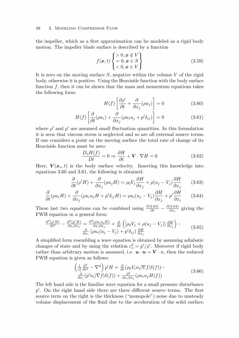
48 3. Modeling Compressor Flow
the impeller, which as a first approximation can be modeled as a rigid bodymotion. The impeller blade surface is described by a function
f(x, t)
> 0,x /∈ V= 0,x ∈ S< 0,x ∈ V
(3.59)
It is zero on the moving surface S, negative within the volume V of the rigidbody, otherwise it is positive. Using the Heaviside function with the body surfacefunction f , then it can be shown that the mass and momentum equations takesthe following form:
H(f)
�∂ρ�
∂t+
∂
∂xj(ρuj)
�= 0 (3.60)
H(f)
�∂
∂t(ρui) +
∂
∂xj(ρuiuj + p�δij)
�= 0 (3.61)
where ρ� and p� are assumed small fluctuation quantities. In this formulationit is seen that viscous stress is neglected and so are all external source terms.If one considers a point on the moving surface the total rate of change of itsHeaviside function must be zero:
DsH(f)
Dt= 0 ⇒ ∂H
∂t+ V ·∇H = 0 (3.62)
Here, V (xs, t) is the body surface velocity. Inserting this knowledge intoequations 3.60 and 3.61, the following is obtained:
∂
∂t(ρ�H) +
∂
∂xj(ρujH) = ρ0Vj
∂H
∂xj+ ρ(uj − Vj)
∂H
∂xj(3.63)
∂
∂t(ρuiH) +
∂
∂xj(ρuiujH + p�δijH) = ρui(uj − Vj)
∂H
∂xj+ p�
∂H
∂xi(3.64)
These last two equations can be combined using ∂(3.63)∂t − ∂(3.64)
∂xigiving the
FWH equation in a general form:
∂2(ρ�H)∂t2 − ∂2(p�H)
∂xi∂xj=
∂2(ρuiujH)∂xi∂xj
+ ∂∂t
�[ρ0Vj + ρ(uj − Vj)]
∂H∂xj
�−
∂∂xi
(ρui(uj − Vj) + p�δij) ∂H∂xj
(3.65)
A simplified form resembling a wave equation is obtained by assuming adiabaticchanges of state and by using the relation c2o = p�/ρ�. Moreover if rigid bodyrather than arbitrary motion is assumed, i.e. u · n = V · n, then the reducedFWH equation is given as follows:
�1c2o
∂2
∂t2 −∇2�p�H = ∂
∂t (ρ0Vini|∇f |δ(f))−∂
∂xi(p�ni|∇f |δ(f)) + ∂2
∂xi∂xj(ρuiujH(f))
(3.66)
The left hand side is the familiar wave equation for a small pressure disturbancep�. On the right hand side there are three different source terms. The firstsource term on the right is the thickness (“monopole”) noise due to unsteadyvolume displacement of the fluid due to the acceleration of the solid surface.

3.5. Ffowcs Williams and Hawkings equation 49
Since most impellers are designed with thin blades, i.e. their volumes aresmall, it means that the thickness noise is often negligible for centrifugalcompressors. The second source term on the right hand side of Eq. 3.66 is theblade loading (“dipole”) acoustic source term. It is associated with unsteadypressure fluctuation on the moving surface. This term is typically the majornoise source for centrifugal compressors. The last source term in Eq. 3.66is related to unsteady Reynolds stress or transport of momentum. It is alsoreferred to as a quadrupole source, but usually insignificant in comparison withthe blade loading term for centrifugal compressor applications. The goal is thento integrate Eq. 3.66 under assumption of no obstacles between the source andthe receiver location. For a more detailed discussion see the works by Farassat(1981).

Chapter 4
Numerical Methods
4.1. Discretization
The governing equations (3.1, 3.2 and 3.3) together with the constitutiverelations describe an inherently complex system consisting of non-linear partialdifferential equations. A major difficulty is the lack of analytical solution(s)for this non-linear system of equations. One may find particular solutionsto the system by making significant assumptions and simplifications. If suchsimplifications and assumptions yield too poor description of the flow, one haveno other option than using numerical methods to solve the equations, whichare believed to describe correctly the physics of the flow. Numerical solutionsrequire discretizing the domain (space-time) under consideration along with theequations. These discretization steps may be done in different ways: the volumecell used in the computational grid may for example have different shapeswith different number of faces. Similarly, the discretization of the equationscan be done using different approximations. A common approach is to uselocal polynomials to approximate the behavior of the dependent variables. Thediscrete approximations can be derived, using various formulations. The bottomline is that the different approaches yield an approximation to the equationswith a residue that is proportional to a power of the characteristic size of thegrid. For example finite differences and finite volumes belong to this classof discretizations. An introduction to numerical methods may be found, forexample in Ferziger & Peric (2012). In the discretization conservation laws,it is natural to go back from the differential formulation to the conservationformulation for a control volume that has the same form as a computational cell.A variable φ, representing specific mass, momentum and energy is introduced.The conservation laws in vector notation are:
∂
∂t
�
V
ρφdV +
�
A
ρφ(v − vsp) · da =
�
A
Γφ∇φ · da+
�
V
SφdV (4.1)
where for mass balance φ = 1, and for momentum balance φ = u, v, w, andfor energy balance φ = e + 1
2v2. Thus, there is integration over individual
finite volume cells, where a is the surface vector of the control volume V . Theterms Γφ and Sφ are associated diffusion and source coefficients, which canbe deduced from the parent equations. One merit of this formulation is that
50

4.1. Discretization 51
the discretized forms preserve the conservation characteristic of the parentdifferential equations. In case of rigid body motion a grid velocity term vsp isincluded for the convection, i.e. the 2nd term on the left hand side. This velocityis simply the relative velocity between the fluid (v) and the surface (vsp). Thefirst term in Eq. 4.1 is the transient term, which is included in LES but isomitted in steady-state RANS computations. The second term expresses theflux of each variable through the face area a of the control volume V due to theflow and due to the motion of the face of the control volume, respectively. Thefirst term on the right hand side is associated with transport of each variabledue to diffusion. For steady state simulations the grid is stationary with vsp = 0.In order to model a rotation due to the impeller motion, one may incorporate avolume (Coriolis) source in the momentum equation.
Sφ = ρω × vrel (4.2)
The balance equation (Eq. 4.1) is cast into a discrete form using a cell-centeredcontrol volume formalism. In discrete form for a cell index O it is given by:
∂
∂t(ρφV )0 +
�
f
[ρφ(v − vsp) · a]f =�
f
(Γφ∇φ · a)f + (SφV )0 (4.3)
where the summation is over all faces f of the control volume. Each itemin the discrete form of the transport equation is subsequently approximatedwith a discretization scheme. Throughout the thesis, the transient term isapproximated with an implicit 2nd order scheme given by:
∂
∂t(ρφV )0 =
3[(ρφV )n+10 − (ρφV )n0 ] + [(ρφV )n−1
0 − (ρφV )n0 ]
6Δt(4.4)
The next term of interest is the convective term. A higher order schemewill give more accurate result. However, higher order schemes may be sensitiveand unstable. A good compromise between accuracy and robustness is the 2ndorder upwind/central scheme, given as:
(mφ)f =
�mfσφf,0 + (1− σ)[fφf,0 + (1− f)φf,1]mfσφf,1 + (1− σ)[fφf,0 + (1− f)φf,1]
�for mf ≥ 0for mf < 0
(4.5)
where σ is a blending factor between upwind or central. Subscripts 0 and 1,respectively, denote two neighboring cells. The face values are then linearlyinterpolated from cell values on either side of the face using reconstructiongradients, via:
φf,0 = φ0 + (xf − x0) · (Δφ)0φf,1 = φ0 + (xf − x0) · (Δφ)1
(4.6)
If the solution is well behaved then it is possible to use higher order schemes, suchas the Hybrid MUSCL 3rd-Order/Central-Differencing scheme. One alterationto the 2nd order scheme is usage of a larger stencil but similar in the sense thatthe σ switch controls the amount of blending with MUSCL 3rd-order upwindcompared to 3rd-order central. Detailed introductions of these schemes can befound in Darwish & Moukalled (1994) and Demirdzic et al. (1993).

52 4. Numerical Methods
Finally, the gradient of fluid property φ in the diffusive flux term is obtainedwith a 2nd order scheme
∇φf = (φ1 − φ0)a
a · (x1 − x0)+∇φ− (∇φ · (x1 − x0))
a
a · (x1 − x0)(4.7)
where ∇φ = (∇φ1 +∇φ0)/2. It can be seen that the discretization employedyields an algebraic system of the non-linear equation system, due to the couplingof the dependent variables within the system. The algebraic system can belinearized by “freezing” the coefficients in between the iterations. For thetransported variable φ at iteration k + 1 becomes:
apφk+1p +
�
n
anφk+1n = b (4.8)
where summation is assumed over all the neighbors n of cell index p. Theright hand side, denoted b is the explicit result obtained at iteration k. Thecoefficients ap and an, respectively, are a result from the discretization process.From this point the transported variable at the next time iteration can beobtained by using Gaussian elimination or LU decomposition. However, forcentrifugal compressor applications, the system is very large making matrixinversion procedures impractical. Instead the unknowns φk+1 are cast into acorrection (Δ) form given as:
apωΔφp +
�
n
anΔφn = r (4.9)
where Δφ is the difference in the transported variable at current k + 1 andprevious k iteration, respectively. The term on the right hand side r is calledresidual, given by:
r = −
∂
∂t(ρφV ) +
�
f
(ρφv · af −�
f
(Γ∇φ · af − SφV
= 0 (4.10)
The residual represents the derivation of the discretized form of the originalequation at iteration k from 0 (i.e. the error in solving the discrete equation).When the discretized equation is satisfied the residual goes to zero. In the thesis,the Gauss-Sediel implicit iterative solution procedure is used. This methodupdates the transported value in each cell using information from cell neighbors.The Gauss-Seidel can be shown to have a faster convergence rate as comparedto the Jacobi method, which is why it is preferred. However, Gauss-Seidelalone is subjected to a very poor computational turnaround. For a discreteproblem with N degrees of freedom (roughly equal the number of grid points)the total work for convergence scales as N2 lnN . Thus, for increasing problemsize the computational effort increases more than quadratically. The idea isthat Gauss-Seidel enables efficient smoothing of local errors. However, it sufferson convergence because it takes time for boundary information to propagateinto the domain. Instead of a large number of Gauss-Seidel sweeps, we use anAlgebraic Multigrid (AMG) algorithm. The concept of the Multigrid algorithmis to handle the error in the solution on a sequence of coarser grid levels.

4.1. Discretization 53
Through this process the boundary information propagates much faster on acoarse grid as compared to a fine grid and thereby the solution is attained muchfaster. The AMG mechanism is thus to alternate the Gauss-Seidel iterationbetween coarse and fine grid levels. This is accomplished by means of transferoperators between coarser and finer grids. Optimally, AMG converges with acomputational work proportional to N lnN , which implies linear growth withincreasing problem size.
The stability condition criterion stipulates that the region of dependence ofthe discretization computational volume should include the region of the depen-dence of the partial differential equations. This translates into the conditionthat information propagating on the grid should not move more than one celllength at a time per time-step. It is a necessary condition and governed by thelocal convective CFL number (Courant-Friedrich-Lewy), which for compressibleflows can be defined:
CFL =(|U |+ c)Δt
Δx≤ 1 (4.11)
It is a function of a characteristic velocity U , the time-step size Δt, the charac-teristic cell with size Δx, and where c is the sound speed. The highest speedsfor rotating machinery problems are typically found near the blade tip region.A subsequent conservative time-step estimate for stability is given as:
Δt =(Δx)tipωRtip
(4.12)
where ω is the impeller angular velocity.
4.1.1. Boundary conditions
Since a centrifugal compressor generates noise, special considerations are neededto allow pressure fluctuation disturbances to propagate freely at the sound speedtowards the farfield. If the centrifugal compressor is fitted with a bell mouthinlet, the upstream flow may be approximately quiescent where stagnationtemperature and pressure are given from ambient reference conditions. Toallow sound propagation then, the correct treatment is to adopt a non-reflectiveboundary condition. A detailed description of non-reflective boundary treat-ments can be found in the works of Giles (1990) and Saxer (1992). In short,the freestream velocity on the boundary is corrected by a combination of thefreestream velocity and the boundary normal velocity component:
�vf = �v∞ + (vfn − v∞n)�a
|�a| (4.13)
where v∞n is the boundary normal freestream component. From characteristicsthe boundary normal velocity vfn is obtained:
vfn =1
2(vr0n + v∞n) +
c0 − c∞γ − 1
(4.14)
where vr0n is the boundary normal velocity component extrapolated from theneighboring cell center. The sound speed c∞ is obtained from the freestream
54 4. Numerical Methods
temperature and c0 is the sound speed obtained from the boundary temperatureas extrapolated from the cell center:
c0 =�γRT r
0 (4.15)
In case of subsonic inflow, the freestream pressure via the isentropic relation isutilized for computing the boundary pressure:
pf = pr0
�Tf
T r0
�cp/R
(4.16)
where the temperature on the boundary face is given by:
Tf =c2fγR
(4.17)
and where:
cf =1
2(c∞ + c0) +
1
4(γ − 1)(vr0n − v∞n) (4.18)
It should be noted that errors can occur with this treatment in the non-normaldirection, i.e. where the boundary is not normal to the incident compressionwaves.
In the experimental setup (Guillou et al. 2012) of the centrifugal compressorinvestigated in this thesis the outlet mass flow is regulated with a lock valve.Such device can influence the flow in such a way that incoming pressure wavesare being reflected. One option to include this effect is to consider a mass flowrate boundary condition. The boundary inputs are a total mass flow rate, totaltemperature and flow direction (in case of flow reversal). As the compressoroperation is towards its surge line, flow reversal may occur. This may potentiallyyield some side effects in scenarios with mixed inflow and outflow on the outletboundary surface. From a numerical stability point of view provisions shouldbe taken to ensure 100% outflow in the boundary normal direction, and this isguaranteed with the mass flow rate boundary condition type.
The specified total mass flow rate is distributed over all faces of the boundaryand a uniform mass flow rate is calculated on each face of the boundary:
mf = mtotal|af |
Σf |af |(4.19)
The static pressure and static temperature, respectively, at the boundary areextrapolated from the interior of the domain. It can be mentioned also thatthe current compressible flow solver has been used previously in the researchgroup Competence Center for Gas Exchange (CCGEx) for solving several fluidflow problems associated with gas-exchange processes and turbocharging ininternal combustion engined applications, see e.g. Semlitsch et al. (2014b, 2015);Semlitsch & Mihaescu (2016).

Chapter 5
Results: Highlights and Discussion
An overview of the centrifugal compressor theory and expected fluid instabilityphenomena occurring under off-design conditions have been discussed briefly inthe previous chapters. Part II of the thesis contains selected papers showingthe main results. Highlights from those papers are outlined in the followingtogether with listing of main researching findings.
In this thesis the main application under consideration has been a vanelessdiffuser centrifugal compressor fitted with a ported shroud, as shown in Fig. 5.1and presented in Papers 1 to 5. However, the same computational tool has alsobeen applied for investigating the stall instability emerging in a vaneless diffuserof a larger centrifugal compressor, without explicitly considering the impellerpresence in the simulations. Instead, the effect of the impeller blade passing isprovided as meridional and tangential velocity profiles, respectively. This caseis presented in Paper 6.
In order to fully characterize the compressor behavior and the developedflow instabilities at off-design conditions, there is a need to accumulate data fora large number of operating conditions. However, one have to keep in mind thatif the target is only to characterize the overall compressor performance (pressureratio and efficiency) as a function of mass flow rate, steady-state RANS basedsimulation is the method of choice (see e.g. Sundstrom et al. (2017a)). If thepurpose, as previously stated, is to look into understanding the flow instabilitiesdeveloped at off-design/unstable operating conditions, and their impact onthe compressor’s performance and noise generation, the LES calculation is themethod of choice. Naturally, due to the required large computational resourceswith such an approach, it is not feasible to cover the entire compressor mapusing LES. For this reason, only selective operating conditions are consideredunder stable and unstable regimes. This choice was made for two differentspeed-lines, c.f. Papers 1 and 3 for further details.
As with any numerical simulation it is always relevant to check the validityof the computed result. Accuracy typically depends on modeling assumptionsbut equally important is the influence from the employed discretization. Thus,one may distinguish between errors and uncertainties in solving the discreteequations, errors in solving the model (PDE) equations and finally the inher-ent uncertainties and possible errors in the model equations themselves. For
55

56 5. Results: Highlights and Discussion
inletoutlet
DO
IS1P2 P1
front section side section
impeller section
r
θz
Figure 5.1: Side and front views of the centrifugal compressor are shown atthe top of the figure. Location of planes used for data post-processing andlocations of the pressure sensors D0 and IS1 are indicated. The IS1 point islocated in the middle of the ported shroud cavity 0.22D2 from the diffuser backwall and oriented 127o clockwise from the vertical. The D0 point is locatedmid of the diffuser channel at radii 55.5 mm and oriented 30o clockwise fromthe vertical. The impeller section intersects the impeller region at 50% bladespan. The P1 and P2 planes are located 0.85D2 and 0.76D2, respectively, fromthe back wall, and oriented with perpendicular intersection of the inlet duct.Subfigures in the bottom part of the figure depict inlet and outlet boundariesof the computational domain. The inset detail at the bottom right illustratesthe blade passage grid resolution at 50% blade span.
historical reasons the scientific community have suggested stages to assess therelevance of numerical results, c.f. e.g. Roache (1998). One necessary step istermed verification. This is a kind of certification process where implementedroutines in the CFD code produce expected result. For example, if the governingNavier-Stokes equations are drastically simplified, e.g. steady-state, 1D/2D,incompressible flow, for an idealized problem scenario, then there can be an

5. Results: Highlights and Discussion 57
exact analytical solution available. The code is therefore setup for such flowscenario and with help of the exact analytic solution the true error is computed.Of course if an analytic solution exists then there is very little need to employCFD. However, for complex problems, e.g. the unsteady flow in a centrifugalcompressor at low-mass flow rates, such an analytical flow solution does notexists. A possibility is to complete a verification of the calculation by assessingthe flow solution’s sensitivity with respect to the numerical, grid and boundarysetups employed, respectively. The other option is called validation, which relieson surveying the relative difference compared to some experimental measure-ment. One problem with validation is that the measured result depends on manyparameters and is subjected also to errors. Moreover, most boundary conditionson the experimental setup are unknown. For these reasons, reasonable goodagreements between experiment and numerical simulations for the consideredscenarios in the current work is challenging.
Any numerical approach relying on the finite volume method is grid de-pendent. Therefore, one idea for checking relevance is to make gradual gridrefinements, i.e. temporally and spatially, and check if relevant quantitiesapproach an asymptotic value. In theory, a fine grid is less diffusive and wouldyield more accurate approximations to the solution of the governing equations ascompared to a coarse grid. Based on this, the strategy in Paper 1 is to comparethe result from three different grids, with different grid refinement levels. Withconsistent discreatization schemes the truncation error should tend to reducemonotonically as the grid size is refined. However, from practical considerations,there is another issue known as round-off error due to finite precision of thecomputer, which may set a lower limit on the grid resolution. In practice, doubleprecision (64-bit) is adequate for practically all CFD computations.
The main outcome from the validation process is the demonstration of thecapability with LES to consistently predict the global performance parametersfor a wide range of operating conditions, as shown in Fig. 5.2. Overall, the resultsof the numerical setup are reasonably close to the corresponding experimentaldata. In the figure the vertical and horizontal bars indicate variations in themonitored signals. Therefore, they are almost not visible for Case D, since thisis approximately a steady-state flow condition. However, as conditions approachlow mass flow rates, a substantial increase can be seen. For Case A, i.e. themost restricted mass flow rate, a limit surge cycle is manifested, associated withsignificant vibrations of the performance parameters.
Regarding the direct comparison with the experimental data; there areseveral sources causing differences. First, measurements at surge operatingconditions are challenging due to the large oscillations in the system. Note thatthe numerical and experimental set-ups are not perfectly identical, being impos-sible to provide complete boundary conditions to the CFD from experiments.Moreover, one has to keep in mind that the experimental flow regulation systemand the driving turbine have not been modeled in the simulations. These are

58 5. Results: Highlights and Discussion
0.00 0.05 0.10 0.15 0.20 0.25 0.30
1.4
1.5
1.6
1.7
A
BC
D
m (kg/s)
p02/p01
0.00 0.05 0.10 0.15 0.20 0.25 0.300.3
0.4
0.5
0.6
0.7
0.8
A
B
C
D
m (kg/s)
Isen
tropic
efficien
cy
ExperimentNumerical
Figure 5.2: The total-to-total pressure ratio (left) and the isentropic efficiency(right) illustrate the chosen operating conditions for the constant speed-line64000 rpm. The variation of the global performance parameters is marked withhorizontal and vertical bars. Case A shows a limit cycle, depicted with a circleand where the arrows indicate the phase direction. Experimental data accordingto Guillou et al. (2012) is added to guide the reader and is displayed with blackdots.
some of the reasons for which a perfect match cannot be obtained between CFDand experiments.
Naturally, there are uncertainties with numerical accuracy. For instance,discreatization errors emanate from approximations to the governing equations,e.g. implicit 2nd order temporal and implicit 3rd order bounded central differ-encing. The dominant error terms of the finite volume method can be relatedto dominant error terms also with a finite difference equation, which is easier toassess analytically. For example, a finite difference equation may be assessed bysubstituting the Taylor series expansion back into the finite difference equation.After rearrangement the resulting so called modified equation is obtained, c.f.Hoffmann et al. (1996). By considering a simple problem e.g. the linear waveequation in one-space dimension various aspects of the finite difference formula-tion may be investigated, such as order of accuracy and stability requirements.If the Crank-Nicolson implicit scheme (2nd order in both space and time) issubstituted into the 1D linear wave equation the modified equation contains aleading odd-order derivative term, which is being truncated. This can give riseto dispersion errors. A possible side effect from dispersion errors can be intro-duction of phase errors and related issues with exactly matching the measuredsurge frequency tonality. If however, an alternative 2nd order scheme such asthe explicit Lax is considered, the formulation may yield a leading even-orderderivative term. Such truncation terms are associated with dissipation errorsand can contribute to amplitude errors, i.e. the initial wave height is diffusedover time.

5. Results: Highlights and Discussion 59
One of the best ways to check the relevance of the numerical approach isto assess if the numerical grid resolution employed is sufficient for capturingessential features of the flow. For this purpose three grids named Coarse,Medium and Fine are run for a reference operating condition. Here selected forω = 64000 rpm at near maximum efficiency condition m = 0.28 kg/s. To see aclear trend due to refinement, a factor of at least two should be employed, seeTab. 5.1. A Courant number unity is not required everywhere in the domainwhen implicit time stepping is employed. Ideally, for accurate time dependentsolution the CFL condition should be obeyed. However, if the grid resolution iswell scaled to the problem then the time-step should be such that the local CFLnumber should be much smaller than unity to allow convergence of the Taylorseries (of the discreatization) and to have the error being composed mainlyof the leading neglected term. In any event, the CFL condition is relevant toensure that information propagates correctly, for example across the slidinginterface between rotating and stationary regions in the computational domain.For a fair comparison the time-step size is adjusted so that the local Courantnumber is similar between grids.
grid cell count Δxi [mm] Δt [deg/time-step]Coarse 0.7 million 2.8 4Medium 2.8 million 1.4 2Fine 9 million 0.7 1
Table 5.1: Characteristics of the Coarse, Medium and Fine grids is listed. Thesecond and third columns tabulates the cell count and the average cell edgelength Δxi for each grid. The chosen time-step Δt used is presented in the lastcolumn. It is given as the number of degrees of impeller rotation per time-step.
It should be noted that a grid sensitivity procedure could be done in manydifferent ways. One option is to extrapolate a solution to an infinitely smallgrid size by means of Richardson’s extrapolation. Richardson’s technique canbe used to find out existence of an asymptotic behavior of the solution. Thismay enable increasing the accuracy (and formal order) without the need toevaluate the solution on an even finer grid. For best outcome it is suggest tostate the quality in terms of several different parameters, see e.g. Celik et al.(2008). For practical reasons the number of analyzed quantities are limited.Here, one preferably chose quantities where experimental data is available. InPaper 1 experimental data was available with respect to the static pressuredistribution at two different radii, see Fig. 5.3.
The essential outcome here is that the Coarse grid depicts some variations,especially at 3 o’clock where the trend with the experiential data is different.As the spatial resolution is improved the trend w.r.t. the experimental dataimproves. The differences between grid levels can be utilized to assess a relative

60 5. Results: Highlights and Discussion
0 100 200 300
Volute angle [deg]
20
25
30
35
40
45
50
55
60Pressure[kPa]
Exp r=55.5 mm
Exp r=72.5 mm
LES coarse
LES medium
LES fine
Extrapolated72.5 mm55.5 mm
0o300o
Figure 5.3: Static pressure distribution in the diffuser obtained experimentally(Guillou et al. 2012) and numerically (LES) with grids Coarse, Medium and Fine.The operating conditions corresponds to Case D at 64000 rpm. The assessmentis performed with points arranged circumferentially around the diffuser andevaluated at two different radial stations, r = 55.5 mm and 72.5 mm. The insetto the right shows measurement probe point locations on the compressor backwall.
error. For any quantity φ this is defined as:
err21 =
����φ1 − φ2
φ1
���� (5.1)
the subscripts denotes the specific grid refinement level. The lower value is forthe finer grid and the larger is for the coarser grid. According Celik et al. (2008)the apparent order oa of the numerical approach is given by:
oa =1
ln(r21)| ln(|�32/�21|) + g(oa)| (5.2)
g(oa) = ln
�roa21 − s
roa32 − s
�(5.3)
s = 1 · sign(�32/�21) (5.4)
where �ij is the difference in φ between grids i and j. For a grid refinementfactor rij of 2 then g(oa) is zero. A solution on a hypothetical infinite resolvedgrid can be computed by means of extrapolation:

5. Results: Highlights and Discussion 61
φext =roa21φ1 − φ2
roa21 − 1(5.5)
which is shown with a thick gray line in Fig. 5.3. This line is seen to beclose with the Fine grid solution. Moreover, the relative error between the finegrid level solution and the extrapolated result can be computed as follows:
errext =
����φext − φ1
φext
���� (5.6)
From Celik et al. (2008) the Grid Convergence Index (GCI) is defined asfollows:
GCI =1.25err21roa21 − 1
(5.7)
which can be used to estimate the uncertainty of the extrapolated result.Results for the GCI and the relative errors are listed in Table 5.2.
errij errext GCIr = 55.5 mm 1.7% 0.5% 0.7%r = 72.5 mm 0.7% 0.07% 0.09%
Table 5.2: Tabulation of grid convergence parameters. The data is based onthe diffuser static pressure distribution at two different radial stations.
Due to low relative errors further grid refinements would therefore only havea marginal effect on the numerical accuracy in solving the governing partialdifferential equations.
Another important assessment is to verify that the grid adequately capturesrelevant frequency tonalities of interest, i.e. as associated with certain fluctuatingflow structures. In Fig. 5.4 the Power Spectral Density (PSD) based on thepressure history signal is presented for different grid resolutions and comparedwith available experiential data. The mid frequency range for conditions closeto near optimum design efficiency is captured by all grids for the chosen diffuserprobe, see Paper 1 for more details. An important tonality is the blade passingfrequency, which is found in the high frequency range. This feature including itshigher harmonics is correctly captured. However, it is only the fine grid level thatgives a reasonable match with the measured data. In the high frequency rangefor the fine grid there is a trend showing an energy decay slope of approximately-7/3. This could be related to Kolmogorov’s energy decay law. However, caremust be taken with any such conclusion because the theory is only valid forisotropic turbulence. Clearly, due to presence of a boundary layer, that is anassumption that may not hold for vaneless diffuser flow. Nevertheless, thelimitation here is mainly due to the fact that the turbulence spectrum and the

62 5. Results: Highlights and Discussion
flow conditions share the same scales. Therefore, classical turbulence theorymay not work fully. For example if the blade passage is pumping energy intothe inertial subrange the classical energy cascade may be disrupted.
103
104
105
Frequency [Hz]
10-2
10-1
100
101
102
103
PSD
[Pa2/Hz]
-7/3
Experiment
LES fine
LES medium
LES coarse
Figure 5.4: Power Spectral Density of pressure for the three grids. For clarifica-tion of the probe D0 location, see Fig. 5.1.
Overall the result with the fine grid shows that the adopted implicit LESapproach has no effect on the frequencies related to the blade passage. Theeffect of grid refinement is manifested in a wider resolved inertial subrange inthe spectrum. As expected, the dissipation occurs mostly at the edge of theresolved scales. With improved resolution the dissipation and a given scale isreduced and thereby the spectrum gets closer to the theoretical one. Furtherrefinement will ultimately result in no effect as the LES with better and betterresolution will become a DNS. This process exhibits the approximate characterof LES, which differs in principle from that of models (like the one used withinthe RANS framework), which do not vanish with improved resolution.
The observed differences between stable and unstable operating conditionscan be expressed in terms of time-averaged velocity and Reynolds stress profilesupstream of the impeller eye, as shown in Fig. 5.5.
In the blade passages, the effect of the higher back pressure is seen topush the flow through the blade tip gap far upstream to the shroud inlet. Forreduced mass-flow rates the amount of back flow increases, as quantified withthe axial velocity profiles for Cases D to A in Fig. 5.5. A strong swirling motioncomponent of the flow in the same rotational direction as the impeller is seen,which is a manifestation of the rotor angular velocity. Therefore, the entireflow upstream of the impeller swirls around the shaft axis and where a mixingtakes place between the blade tip gas flow with the freshly entrained air flow.The increased mixing of flow in this local region towards off-design operating

5. Results: Highlights and Discussion 63
0 0.1 0.2−1
−0.5
0
0.5
1
Ur/Uref
r/R
ABCD
0 0.1 0.2
Uθ/Uref
0 0.1 0.2
Uz/Uref
0 5 · 10−2 0.1 0.15−1
−0.5
0
0.5
1
�u�ru
�r/Uref
r/R
0 5 · 10−2 0.1 0.15�
u�θu
�θ/Uref
0 5 · 10−2 0.1 0.15�u�zu
�z/Uref
Figure 5.5: Time averaged velocity and Reynolds stress profile components inradial, tangential and axial directions. Data is extracted along a vertical line inplane P2. The profiles are normalized with the blade tip speed, Uref . The grayhorizontal lines indicate the circumferential radius at which the rotating-stallvortical structures are circulating in the P1 plane. This location is in nearproximity of the inflection point. Cases A to D correspond to those markedwith the same symbols in Fig. 5.2.
conditions can therefore be seen as amplified turbulent kinetic energy levels. Adistinct shape of an annular separated formation can be seen in the P2 plane(shown in the Ur/Uref subplot in Fig. 5.5). It is manifested as radial outwardsand inwards swirling flow which is a consequence due to the significant amountof back flow. It can be seen as a blockage or obstacle for the entrained airfurther upstream. Thus, the freshly entrained air is being funneled into thecompressor with a radial inward directed flow profile (the radial velocity profilesare shown in Fig. 5.5). The back flow on the other hand is seen to spread

64 5. Results: Highlights and Discussion
outwards due to the centrifugal forces but is concentrated towards the shroudside. When considering the radial and the axial velocity profiles together it isclear that an inflection point emerges for Case C, which grows for the lowermass flow rate Cases B and A. In general the flow in the inflection point maybe unstable and so it is a possible onset mechanism for shear-layer instability.One effect of the shear-layer interface can be seen as an annular region withincreased turbulent kinetic energy.
The thesis focuses on low-frequency flow phenomena, rotating stall andsurge. Hence, there is no intention to capture the smallest scale turbulent flowfeatures. This option is viable if the phenomena under consideration are notturbulence driven, but are results of other factors, such as system rotationand inertia. The phenomena, rotating stall and surge are subjected to ordersof magnitude larger length scales but more importantly longer time scales ascompared to the blade passing frequency. Consequently such features require anadequate number of time samples, with relatively low sampling rate, such thatthe frequencies of interest can be resolved. Therefore, a significant statisticscorresponding to some 220 full impeller revolutions were accumulated for CaseA and run on the fine grid. Of this approximately, 20 revolutions are neededfor the early transient evolution from RANS to establish a suitable initialturbulent flow field. Therefore, data corresponding to 8 surge periods are usedfor statistical analysis of Case A. Since the low frequency tonality correspondingto surge was not expected for Case B, C and D, respectively, a fewer number ofimpeller revolutions were considered, but corresponding to 2 surge periods. Onemay note the fact that the phenomenon under consideration has long lengthscales, which implies that the effects of turbulence on surge and rotating stallare small.
The corresponding Power Spectral Density (PSD) for the audible frequencyrange is presented in Fig. 5.6. Spectra at probe point IS1 is assessed alongone speed-line and the purpose is to evaluate differences as conditions go fromnear maximum design condition Case D to off-design condition at Case A. ForCase D the major tonalities that are distinct and clear are found at RO = 1,RO = 5 and RO = 10. Here the blade passing frequency (BPF) equals RO =10, since the impeller has ten blades. Elsewhere the spectrum is broadbanded.As the mass flow rate is restricted in Case C, no spectacular change is seen,except perhaps, a small bump appearing for a frequency range around half theangular velocity of the shaft (i.e. RO = 0.5). For Case B, the mass flow rateis even more restricted. Suddenly a notable low frequency tonality occurs atRO = 0.5, which is identified as rotating stall. In the previous Case C andCase D such feature cannot be distinguished. For Case A, yet another lowfrequency tonality is manifested at a fraction of the rotating order (43 Hz).This peak is also accompanied by one higher harmonic in the numerical data.One interesting observation for this particular centrifugal compressor is thatthe rotating stall tonality is still present under deep surge conditions. However,for Case A the spectra indicate that the rotating stall feature operates over a

5. Results: Highlights and Discussion 65
101
102
103
104
105
PSD
(Pa2/Hz)
Case A
-7/3
Case B
10-1
100
101
RO
101
102
103
104
105
PSD
(Pa2/Hz)
Case C
10-1
100
101
RO
Case D
Experiment
Numerical
Figure 5.6: Power Spectral Density (PSD) for Cases A to D. The data is basedon the pressure time history in probe location IS1 (see Fig. 5.1 for orientationpurposes). Experimental data (Gancedo et al. 2016) is added as a reference. TheRotating Order (RO) on the abscissa is a frequency normalized with the angularvelocity of the impeller shaft. A one full impeller wheel rotation corresponds toRO = 1.
wider frequency range, i.e. gaining a hump characteristic rather than a sharptonality. Based on the computed result the crucial factor leading to surge isthe global response due to flow recirculation causing the emptying and fillingprocess. To quantify the compression system it is therefore needed to lookat the phase locked average incidence angle variation at leading and trailingedges of the impeller blades. The motivation is that flow incidence can beseen to influence the impellers ability to push fluid downstream and hencebuild up boost pressure. A quantitative representation of cycle phase averagedflow angles, flow momentum and total-to-total pressure ratio, respectively, aretherefore presented in Fig. 5.7. The effect of large-scale flow structures on theblade loading term can be analyzed by filtering the flow field and blade loadingterm at a particular frequency. Figure 5.8 shows the phase angle evolutionΦ, of the reconstructed acoustic blade loading term (top row) for off-designoperating condition at the low surge frequency tonality. This figure is thereforea good complement to Fig. 5.7, since the connection between flow and acoustics

66 5. Results: Highlights and Discussion
is included. It shows how the coherent flow structure in surge affect the bladeloading term, which in turn affects the momentum flow into the radial diffuserfor one complete surge cycle.
By phase angle Φ = 0 the streamlines indicate that the flow is being pushedmainly downstream, see Fig. 5.8. Thus, the turbulent kinetic energy levelreaches a minimum level. However, the back pressure is at a maximum, whichinduces more recirculation in the volute region, see Fig. 5.7. As an effect theflow incidence angles therefore increases while the upstream and downstreamflow momentum decreases. Since the back pressure is at its peak level thecorresponding blade loading distribution shows a maximum towards the rearpart of the impeller surface. However, referring to a downstream directedflow is not completely satisfactory since the streamlines close to the bladesuction side describes a circulating motion. There, the streamlines are seen tospiral outwards initially prior discharge. Qualitatively, this feature outlines anemerging boundary layer separation, and is associated with a strong adversepressure gradient. By phase angle Φ = π/2 later, all seeded streamlines inFig. 5.8 indicate upstream direction. This means that the compressor is enteringthe emptying phase of the surge cycle and the flow is completely reversed. Fromthis point in the phase cycle the pressure reduces rapidly. The turbulent kineticenergy manifests a strong gradient in the blade passages. A consequence ofcomplete flow reversal is that the impeller cannot produced any observabledownstream momentum (Fig. 5.7 at Φ = π/2).
In this condition the impeller cannot retain its efficiency. A phase shiftof π/2 is observed between the pressure and the flow momentum indicatinga resonance phenomenon. By phase angle Φ = π the turbulence level hasrelaxed yet the seeded streamlines depict complete flow reversal. However, theupstream streamlines are almost parallel with the inducer plane. Therefore, thecompressor is gradually undergoing a recovery from its minimum pressure levelof the mode cycle.
At Φ = 3π/2 the compressor is subjected to the filling phase of surge.The corresponding blade loading term depicts a neutral level. By phase angleΦ = 3π/2 the compressor is recovering where the flow is now being directeddownstream again. Therefore, the flow incidence angles reach a minimum andsubsequently the flow momentum transferred downstream reaches high values(Fig. 5.7 at Φ = 3π/2). The flow mode perturbation transition from Φ = 3π/2to Φ = 2π can be seen as an adjustment back to the phase evolution describedat Φ = 0. From this point the phase evolution will repeat in a surge limitcycling procedure. The cyclic behavior of the blade loading pressure is hereseen as the acoustic source mechanism responsible for amplified noise levels inoff-design operating conditions.
Another important low frequency phenomena observed in the computedLES data is associated with rotating stall. Figure 5.9 shows the phase angleevolution, Φ, of the flow perturbation and the blade loading term contributionat RO = 0.5.

5. Results: Highlights and Discussion 67
0 π 2π0
2
4
6
8
10β1−β1b(o)
0 π 2π2
4
6
8·10−2
(ρu2 z1)/(ρ
refU
2 ref)
ABCD
β1
β1b
β2b
β2
0 π 2π10
20
30
40
50
Φ
β2−β2b(o)
0 π 2π0
0.1
0.2
0.3
0.4
Φ
(ρu2 r2)/(ρ
refU
2 ref)
0 π 2π1.5
1.55
1.6
1.65
1.7
Φ
p02/p
01
Figure 5.7: Impeller performance quantity characteristics are presented for CasesA to B. The data is phase cycle averaged based on the dominant frequency foreach case: Case A, surge; Case B and C, rotating stall; Case D, time-averaged.Flow angles and flow momentum at the inducer and exducer including thetotal-to-total pressure ratio are circumferentially averaged at 50% blade span.The inducer blade angle is β1b = 60o and the blade back sweep angle is β2b = 40o.These angles are defined relative to the meridional, see sketch in the upper rightcorner.
It should be noted that the rotating reference frame rotates with RO = 1,which is clockwise in Fig. 5.9. An observer in the acoustic farfield is locatedin an absolute frame of reference, which does not move. Thus, it is vital totransform the observations between moving and non-moving reference frames.The flow quantities pressure and velocity in the impeller region are sampled inthe rotating reference frame in cylindrical coordinates. For an interpretationin a static (absolute) frame they should be rotated in the other direction byangular velocity RO = -1. In rotating stall a stationary observers would see theupstream vortices rotate at RO = 0.5. Hence, RO = 0.5 (absolute) equals RO= 1.5 (rotating) and subtracting RO = 1 reference frame mode. In theory, therecould be a right running and a left running mode contributing to the RO =0.5 (absolute). It may be argued that the acoustic observer cannot distinguish

68 5. Results: Highlights and Discussion
−5.00 0.00 5.00
p�L
0.5ρrefU2ref
· 10−2
Φ = 0 Φ = π/2 Φ = π Φ = 3π/2
0.00 0.06 0.12
�u�r2+ u�
θ
2+ u�
z2/Uref
Figure 5.8: Acoustic blade loading term (top row) and the modal flow pertur-bation (bottom row) at the surge frequency RO = 0.04 for off-design conditionCase A. The sequence from left to right shows the phase evolution of the surgemode shape.
between right and left running disturbances, in the case of a compact source.Thus, for the acoustic point of view RO = -0.5 (absolute) may also be obtainedfrom RO = 0.5 (rotating) minus RO = 1 of the reference frame mode. Hence,another viable noise source emitting due to rotating stall. For the investigatedcentrifugal compressor under consideration, the right running mode RO = 0.5(absolute) turns out to be an order or magnitude larger as compared to theleft running more at RO = -0.5 (absolute). Therefore, the left running mode isnegligible. In Fig. 5.9 the mode depicted with streamlines spin with RO = 0.5clockwise. Thus, impeller surface with the blade loading distribution is rotatedto enable a comparison to the spatial flow field in absolute frame as presentedin the lower part of Fig. 5.9.
In the P1 plane upstream of the impeller, circulating vortical structurescan be observed, which have been identified as rotating stall. These vorticalstructures are cropped by the blades causing high amplitude contributions tothe blade loading term at the leading edge and pressure side of the blade. This
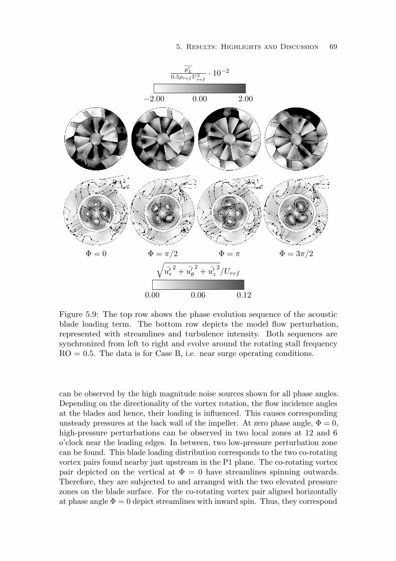
5. Results: Highlights and Discussion 69
−2.00 0.00 2.00
p�L
0.5ρrefU2ref
· 10−2
Φ = 0 Φ = π/2 Φ = π Φ = 3π/2
0.00 0.06 0.12
�u�r2+ u�
θ
2+ u�
z2/Uref
Figure 5.9: The top row shows the phase evolution sequence of the acousticblade loading term. The bottom row depicts the model flow perturbation,represented with streamlines and turbulence intensity. Both sequences aresynchronized from left to right and evolve around the rotating stall frequencyRO = 0.5. The data is for Case B, i.e. near surge operating conditions.
can be observed by the high magnitude noise sources shown for all phase angles.Depending on the directionality of the vortex rotation, the flow incidence anglesat the blades and hence, their loading is influenced. This causes correspondingunsteady pressures at the back wall of the impeller. At zero phase angle, Φ = 0,high-pressure perturbations can be observed in two local zones at 12 and 6o’clock near the leading edges. In between, two low-pressure perturbation zonecan be found. This blade loading distribution corresponds to the two co-rotatingvortex pairs found nearby just upstream in the P1 plane. The co-rotating vortexpair depicted on the vertical at Φ = 0 have streamlines spinning outwards.Therefore, they are subjected to and arranged with the two elevated pressurezones on the blade surface. For the co-rotating vortex pair aligned horizontallyat phase angle Φ = 0 depict streamlines with inward spin. Thus, they correspond

70 5. Results: Highlights and Discussion
to vortical spiraling around low pressures. This correlates with the blade loadingdistribution, i.e. the two low pressure zones aligned horizontally. From Fig. 5.9it is also clear that a similar distribution resides towards the blade trailing edgesat the same phase angle. However, at the exducer the distribution of the twohigh and two low pressures zones, respectively, are not perfectly symmetric.One of the low pressure zones is seen to dwell toward 5 o’clock for other phaseangles, whereas the other low pressure zone on the opposite side is clearlyconvected around circumferentially. The presence of the asymmetry is onepossible motivation of the subharmonic tonality found at RO = 0.25 in thepower spectra density (see Fig. 5.6). This asymmetry can also be related to theasymmetric time averaged pressure field at off-design operating conditions. Dueto this pressure perturbation distribution, the flow is discharged with accordingto these perturbations into the radial diffuser. The streamlines indicate thedirection of the flow perturbations, where a radial outwards and inwards flow inthe diffuser can be related to the locations of high and low pressure perturbationzones at the exducer. A phase angle Φ = π/2 later in the rotating stall cycle,the impeller surface is subsequently rotated the same amount in the clockwisedirection. It is important to recognize that the pressure distribution only rotatehalf as much, i.e. π/4 also in the clockwise direction. Thus, for one full impellerrevolution the rotating stall feature with its blade loading signature only rotatehalf a revolution. This spinning motion in the clockwise azimuthal direction(i.e. absolute frame) explains the RO = 0.5 tonality found in Fig. 5.6. By aphase angle Φ of π further in the cycle, the two high pressure zones near theblade leading edges are seen to be rotated into a horizontal orientation. Furtheron until phase angle Φ = 3π/2 they are therefore seen aligned diagonally, i.e.between 10 and 4 o’clock. From this phase angle instant until 2π both bladeloading distributions and the flow field distribution depicted with streamlinesin Fig. 5.9 will gradually come back to the starting point at Φ = 0. Once backto the starting point, the rotating stall will repeat in another cycle.
Another research highlight emerged from assessment of two-point crosscorrelation along a circumferential line around the middle of the diffuser channel,see Fig. 5.10. The practicality of the method is to compute coherence of theflow fluctuations. The data based on pressure for Cases B and D shows severalinclined diagonal disturbances. There is one line for each fluctuation disturbancedue to the blade passing. The slope of the incline indicates the group speedof the disturbance and is found to be a little higher than the speed of soundat ambient conditions. This is because the group speed gains an additionalcontribution from the convected flow velocity. For Cases A and B, i.e. towardslow mass flow rate operating conditions, the two-point correlation (i.e. Fig. 5.10based on circumferential velocity) is modulated by a low-frequency components,which is due to rotating stall. The effect of the rotating stall is seen to yield twodisturbances convected around the diffuser for Case A and B. They correspondto two crests where the correlation is at a maximum. In between there arevalleys, i.e. maximum correlation but with a negative sign. It is importantto acknowledge the circumferential variation, which suggests that the rotating

5. Results: Highlights and Discussion 71
stall depends on the clockwise orientation. For instance, between positions 12o’clock and under the volute tongue the rotating stall incline is clear, indicatinga speeding up behavior. After the volute tongue an apparent slowing downprocess is seen. For angles on the opposite side of the compressor, i.e. towards8 o’clock, the characteristics are more diffuse showing possible checker-boardpattern. Such feature can be due to the flow being locally subjected to staticstall locally with back and forth motion rather than rotational. For the mostrestricted mass flow Case A, the characteristics based on pressure correlationdisplay horizontal lines. Since those lines do not show any dependence in timethey are immediately recognized as a pattern due to a standing wave andtherefore representing surge operating conditions.
It is well known that centrifugal compressors are subjected to significanthydrodynamic pressure fluctuation levels, c.f. Gonzalez et al. (2003); Broatchet al. (2015). It is located mainly in the impeller region and they are inherently ofhigher magnitudes as compared to acoustic sound waves. From the compressorimpeller, which is influenced by significant hydrodynamic structures, there willbe a decay behavior where the averaged pressure fluctuation level reduces. Fromclassical acoustic theory, and also supported with the LES data (Paper 3 and4), it can be shown that the decay rate in the near-field is inverse proportionalto the square of the distance from the source. For larger distances the influencefrom the hydrodynamic structures diminishes, and the pressure fluctuationsbehave inverse proportional to the distance from the source. Ultimately, thereis a notable change in decay rate, which can be used to distinguish the nearfieldfrom the farfield flow regimes. For the investigated centrifugal compressor thisis located close to the bell mouth entrance, which hence defines the area wherethe acoustical sound field begins.
According to the Lighthills acoustic analogy and assuming flow pulsationin a straight pipe it can be show that the radiated power scales as:
Wm ∝ ρ0f2U2D2
c0≈ 10−4ρ0MU3D2 (5.8)
where ρ0 - air density, f - pulsation frequency, U - mean flow speed, D - pipediameter, M - Mach number, and c0 - speed of sound, c.f. Abom (2006). Inorder to obtain the last expression it is here assumed that the frequency f isclose to the surge frequency. It can be roughly estimated as one hundredthof the rotating order (RO). A source that behaves as a dipole, in centrifugalcompressor applications, is due due to the rotating blade forces. For this termthe frequency f is assumed to be equal with the rotating order. Subsequently,the dipole power scales as:
W d ∝ ρ0M3U3D2 (5.9)
Viscous forces are known to influence the damping of sound waves. Theyemerge from the Lighthill stress tensor and are associated with quadrupolefields. Lighthill showed that the quadrupole radiated power scales as:
W q ∝ ρ0M5U3D2 (5.10)

72 5. Results: Highlights and Discussion
Case A Case B Case D
0
20
40
t(ms)
0
5
10
t(ms)
0
1
2
t(ms)
-π 0 π
θ
0
5
10
t(ms)
-π 0 π
θ
0
5
10t(ms)
-π 0 π
θ
0
1
2
t(ms)
r = 60 mm
θ = 0
Figure 5.10: Two-point cross-correlation for Cases A, B and D. Data is evaluatedalong equidistant and azimuthally arranged points at diffuser radii r = 60 mm.The top row shows cross-correlation based on pressure whereas the bottom rowis based on circumferential velocity fluctuations. The circumferential line startsand ends on the vertical position at θ = 0, i.e. at 12 o’clock. This location isalso used as the reference point, a sketch inset is added for orientation purposes.
Putting the result from the monopole, dipole and quadrupole power terms,respectively, together shows the following relationship:
Wm : W d : W q ∝ 10−4 : M2 : M4 (5.11)
For low-subsonic flows, it can be concluded that the radiated power fromthe dipole radiation term is several orders more significant as compared tomonopole and quadrupole terms. It must be realized that the result obtainedfrom Lighthill’s acoustic analogy is only possible with introduction of strongassumptions. Care must be taken to adopt the result for centrifugal compressors.To clarify the relative importance on the acoustic intensity level from the

5. Results: Highlights and Discussion 73
individual source terms, the spatial distribution are shown in the vicinity of theimpeller, see Fig. 5.11.
p�L, scale = 0 - 0.1 p�T , scale = 0 - 1e-6 p�Q, scale = 0 - 5e-5√
p�2
0.5ρrefU2ref
Figure 5.11: Acoustic intensity level distribution for off-design operating condi-tion Case A. Surface contributions from the blade loading p�L and the thicknessp�T source terms are shown on the impeller wall boundary. The quadrupole p�Qis a volume source term and presented on the 50% blade span section.
It is observed that the computed blade loading term, p�L, contributes tomost of the sound pressure level by an order of magnitude compared to thethickness and quadrupole terms. It is induced by the impeller and represents theinteraction with flow structures primarily found at the leading and trailing edges.There, the blade loading term manifests elevated levels due to the cropping up ofunsteady flow structures. The thickness term, p�T , is more pronounced towardsthe impeller blade tips, which is due to the higher rotational surface velocity.It is known from Raitor & Neise (2008) that tip clearance noise increases asthe tip-speed approaches the sonic speed. For the considered subsonic flowregime in Case A, the influence from p�T is thus small and even seen to be theleast influential. The last acoustic source term considered in Fig. 5.11 is thequadrupole term p�Q. It is associated with turbulent fluctuations in the volumeflow causing acoustic noise propagation. Elevated intensity magnitudes areobserved located in the wake flow zone towards the exducer. The generationmechanism may be associated with strong gradients and large fluctuations, whichare associated with the sound generation. The amplified intensity coincide withthe mixing zone between the separated boundary layer flow towards the bladesuction side and with the higher jet like flow zone towards the pressure side.

Chapter 6
Conclusions
The LES approach has been employed with the purpose to predict the unsteadyflow field in a ported shroud centrifugal compressor equipped with a vanelessdiffuser. Boundary conditions and specifics related to the numerical setup werechosen to be close replications of the cold gas-stand experimental setup atUniversity of Cincinnati. Hence, direct comparison has been possible in terms ofglobal performance parameters but also in terms of flow variables (time-averagedpressure and velocity as well as pressure based spectra). The computed resultswere found to be in good overall agreement with measured data for a range ofoperating conditions. For the considered geometry in this study the mass flowrate was gradually reduced from design (near optimum efficiency condition)to off-design operating conditions with the purpose to provoke low-frequencyinstability tonalities. Narrowband tonalities emerged in the low frequency rangeof the pressure spectra associated with rotating stall and surge. These modeswere assessed by means of flow mode decomposition.
6.1. Contributions
It was found that a growing reversed swirling back-flow emerges as the operatingconditions approach the unstable range. This is in agreement and complementsthe investigations made by other researchers, c.f. Guillou et al. (2012) andHellstrom et al. (2012). The main reason for the back-flow can be attributed tothe high back-pressures at low mass-flow rate. It has been demonstrated that theswirling annular back-flow is intrinsically linked with the alteration of incidenceflow angles. It influences the rotor efficiency due to the reduced entrainmentflow momentum. For more extreme conditions (even lower mass flow rates)the deep surge instability is triggered. In such scenario both downstream andupstream flow momentum transfer are seen to oscillate in a limit cycle loop,which manifest in total pressure ratio pulsation between compressor inlet andpipe discharge.
The surge limit cycle behavior was found to be linked with a phase shiftbetween the pressure ratio and the flow momentum. In detail the peak pressureratio is phase shifted 90o ahead of when the flow momentum approaches itsminimum level. Additionally, it was also found that the incidence flow angleis synchronized with the flow momentum. For example, a large incidence
74

6.1. Contributions 75
angle corresponds to a minimum flow momentum where the pressure ratio istransitioning towards a minimum level in the surge cycle. As the back pressuredecreases, the compressor gradually recovers and is able to gradually buildup theflow momentum again. However, at some critical pressure ratio the momentumwill gradually drop and the surge limit will repeat in another cycle.
The back-flow streaming over the blade tips is seen to reach far upstreamfor all the unstable, low mass-flow rate operating conditions, and hence interactwith the freshly entrained air flow at the inducer. A distinct interface is thereforedeveloped yielding a strong shear-layer. This shear-layer is seen to be energizedby the swirling annular back-flow emanating near the shroud walls and offthe ported shroud cavities. At the inner side of the shear-layer interface itselfhelical vortices are seen to take shape going into spiraling trajectories aroundthe impeller axis. It was found that tip-leakage yielding reversing back-flow atthe impeller eye is intrinsically linked with occurrences of both rotating stalland surge. The rotating stall can be seen to be governed by the shear-layerstrength whereas surge is more affected by the swirling motion as induced by theback-flow. Quantified Reynolds stresses upstream of the impeller eye exposedamplified levels close with the inflection point and thus connecting shear-layerstrength with the mass flow rate.
Since the flow is seen to separate near the shroud wall and reversing inthe upstream direction, it induces a strong shear-layer interface. It was foundthat streamlines curl up into two co-rotating vortex pairs, when seeded closeto the interface. This is a flow instability seen to be relatively distinct inthe point spectra for near surge conditions. However, for more extreme deepsurge conditions the rotating stall feature is seen to fluctuate over a rangeof frequencies. Thus, the co-rotating vortex pair is modulated in presence ofstrong swirl. The narrowbanded feature of the rotating stall instability canalso be traced further downstream in the radial diffuser and volute regions,respectively. Towards off-design conditions it is known that the static pressurescalar distribution in the diffuser gains an asymmetric configuration. This canbe seen as a developing low pressure zone under the volute tongue, caused bythe presence of a small recirculating region. The induced pressure oscillationdue to the convected rotating stall cells in the diffuser are naturally interactingwith the developed recirculation region (and the shear-layer) under the volutetongue region. In other words there is a modulation of the circumferential waveunder the volute tongue, which influences the boost pressure.
Another outcome of the computed unsteady flow is the possible connectionbetween identified flow instabilities and the generated acoustic sources. Afore-mentioned narrowband tonalities as found in the sound power level spectrafor far-field points were correlated with acoustic source terms based on theFfowcs-Williams and Hawkings (FWH) formulation. It was found that the bladeloading term is several orders of magnitude larger as compared to thicknessand quadrupole terms, respectively. The blade loading source term on theimpeller surface, which is dipole in character, has been quantified and exposed

76 6. Conclusions
at frequencies of interest, using the mode decomposition techniques. When theacoustic power from blade loading and quadrupole terms are compared it wasfound that their respective scaling indicates a ratio one over the Mach numbersquared (i.e. Wd : Wq ∼ 1 : M2). This appears to hold in the subsonic Machnumber flow regime. A similarity can be seen with the theoretical power scalinglaw for pulsating pipe flow via Lighthill’s acoustic analogy. It was shown thatthe monopole term is insignificant for the emitted sound for the consideredapplication. However, for higher speed-lines and at larger mass-flows, this termmay become more important, as the flow of the blades is expected to reachsonic speeds, see e.g. Raitor & Neise (2008).
Since the blade loading term was shown to be the most influential soundsource the associated distribution on the impeller surface was assessed by meansof modal decomposition. The first clear occurrence of a rotating stall tonalityin the SPL spectra was detected in the second most restricted mass flow rateconsidered. For this case, the RO = 0.5 mode shape described a typical dipoledistribution. This acoustic signature is seen to be correlated with the co-rotating vortex pair interacting upstream of the blade leading edges. Moreover,an asymmetry pressure loading resides towards the rear of the impeller surface.A higher momentum flow is manifested towards 5 o’clock acting as a low pressuresink. This region becomes amplified towards surge operating conditions. Itcan explain why the rotating stall tonality gains a hump feature in the PSDspectrum and provokes the subharmonic RO = 0.25 tonality.
The SPL spectrum in the upstream far-field for the most restricted mass flowrate considered expose a distinct tonality at the surge frequency and it correlateswith a coherent blade loading feature distributed on the impeller surface. Sinceit emerges from the blade loading term in the FW-H equation it is linked witha dipole acoustic source mechanism. However, the distribution on the impellersurface does not expose a conventional dipole feature in comparison with themode found at the rotating order or the rotating stall mode. Nevertheless, itcan be characterized with a multipole expansion consisting of two monopolesin anti-phase for each impeller blade. They are distributed symmetrically in acircumferential arrangement with focus towards the rear part of the impellersurface as well as towards the leading edges and blade tips. Overall, thedistribution clarifies a possible acoustic source mechanism responsible for theamplified sound pressure level at a fraction of the rotating order frequency.Ultimately, the frequency tonality associated with the surge mode was shownto describe a filling and emptying process between the impeller inlet and pipeexit discharge.
The SPL spectra in the acoustic far-field upstream of the compressor wasseen to contain a second amplified feature located in the mid frequency range.This feature is demonstrated to expose more broadbanded characteristic. How-ever, distinct narrowbanded features are embedded at twice the rotating orderunity, including higher harmonics notably at RO = 3 and RO = 4. This humpfeature in the SPL spectra shares resemblance with experimental observations

6.2. Proposal for future work 77
(Tomita et al. 2013; Evans & Ward 2005), designated as “whoosh noise”. Com-peting explanations exist for the mechanism behind the “whoosh noise” feature.In e.g. Torregrosa et al. (2014) it is associated with a general broadband noisein range 1 < RO < 2 for a similar sized compressor. In Raitor & Neise (2008)it is related to “tip clearance” noise due to flow leakage between the blade tipand shroud wall. Since the time-average pressure scalar distribution aroundthe diffuser and volute regions manifest increasing asymmetry it influences theemitted noise. It is seen to amplify the broadbanded acoustic noise level in theorder of 2-4 dB. Embedded in this broadbanded characteristic there are featuresassociated with the rotating order and its higher harmonics. From an acousticpoint of view they can be defined by dipole sources distributed circumferentialaround the impeller surface.
The main achievements of thesis can be summarized in the following mainpoints:
• The low frequency flow modes associated with surge and rotating stallwere captured with the adopted LES methodology.
• From flow mode decomposition using either Fourier surface spectra orDynamic Mode Decomposition it is possible to describe Surge as a systeminstability. Small disturbances grow until state space variables enter asurge limit cycle.
• It was found that rotating stall can co-exist with the surge feature.However, its tonality spreads over a wider frequency interval.
• The acoustic sources caused by the unsteady pressure loads on the im-peller’s surface have been correlated with the acoustic spectra calculatedupstream of the compressor in the acoustic regions.
• A dominant flow feature at half of the rotating order was identifiedupstream of the impeller inlet face. It was found that the feature consistsof two co-rotating vortex pair circulating in the same direction as theimpeller rotation.
• The generation mechanism of surge was shown to be subjected to largemodulation of incidence flow angles and the impact on the transferredflow momentum through the blade passages.
6.2. Proposal for future work
It has been suggested by different research groups that the tip clearance noiseshould manifest in a narrowband range about half of the rotating order. Earlyinvestigations of “tip clearance noise” can be traced to the axial compressorcommunity. It is acknowledged that rotating stall may evolve differently in acentrifugal compressor, yet this definition has been adopted also for centrifugalcompressors. Since the tip clearance noise is not yet fully understood it wouldbe most valuable to determine the underlying generation mechanism. It istherefore proposed to clarify the generation mechanism that is responsible forthe radiated narrowbanded noise. In other words, determine if it is related to tipclearance or not. The definition that tip clearance noise strongly correlates with

78 6. Conclusions
half of the rotating order originates from experimental studies carried out in the50-70s. Researchers back then did not have access to powerful computers, andthe possibility to visually exploring the entire unsteady flow field was limited.It is identified in this thesis that the coherent flow structures found upstreamof the impeller face illustrate a different flow mechanism. Since detailed flowvisualization by means of experimental measurements is challenging it mayexplain why a tonality found in the power spectra density may be interpretedas a rotating pressure signature for rotating stall. In reality though, it may berelated to a different thing altogether.
It is important to realize that surge and rotating stall are dynamic evolvingflow instabilities. Therefore, the assumption of a fixed speed-line and a specifiedmass flow rate limits the possibility to find the inception mechanism. For higherfidelity prediction of the low-frequency tonalities it is recommended to assess adynamic evolution from design conditions towards unstable off-design conditions.This may help locate a specific operating condition for which a precursor flowmode may occur prior to rotating stall and surge.
The solver elapsed time with LES for one operating condition is in theorder of days running on modern supercomputing hardware facility. This meansthe LES computational approach is not an attractive choice for evaluation ofcompressor performance in early compressor design stages. As a future directionit would be possible to consider unsteady RANS (URANS). It is believed thatURANS may be capable in capturing some of the instabilities observed forunstable operating conditions. Capture of self-induced rotating stall in realisticcompressor geometries on the other hand may demand special considerationswith URANS, such as anisotropic turbulence and curvature correction. However,if the interest is to capture mechanisms related with the noise generation incompressors a URANS formulation may not be a method of choice (due to theimpact of modeling on velocity and pressure fluctuations).
Relying on direct sound propagation with compressible LES is challengingat larger distances from radiating noise sources. It is due to having a sufficientnumber of grid points to resolve the wavelength of acoustical propagating soundwaves. Using the FW-H equation is one option to reduce the computational costassociated with far-field sound propagation. However, in the present formulation,it is mainly suitable for compact acoustic sources. Moreover, all acoustic sourcesurfaces and neighboring volume should be in a direct “line-of-sight” and separatefrom the receiver location. In most radial compressor applications the voluteand shroud surfaces are effectively shielding the dominant acoustic impellersurface source, introducing interference effects. However, results presented inthe thesis exposed that FW-H can give good trends as compared with the directapproach in the low to medium frequency range. However, for more accurateprediction a future direction may explore the integration routines of the acousticsource terms on the right hand side of the wave propagation equation whenapplied to radial compressor applications.

6.2. Proposal for future work 79
Another possible research direction is to asses compressor sensitivity to theupstream and downstream perturbations (e.g. Exhaust Gas Recirculation - EGRpulses, air temperature conditions, pressure pulses caused by engine breathing)and analyze the impact of such perturbations on the onset of compressorinstabilities.

Chapter 7
Publications
As part of the outcome with the current PhD study, several manuscripts werepublished or submitted for publication. They are reproduced in Part II of thethesis and listed as follows:
Paper 1 Assessment of the 3D Flow in a Centrifugal compressor using Steady-State and Unsteady Flow Solvers. Sundstrom E. (ES), Semlitsch B. (BS) &Mihaescu M. (MM) SAE Technical Paper, 2014-01-2856, (2014)
A grid dependency assessment was carried out on RANS and LES data obtainedfor a ported shroud centrifugal compressor. Characteristic low frequency tonali-ties were captured with LES. They were identified as rotating stall and surge bymeans of advanced post-processing techniques. The candidate (ES) performedall pre-processing, solve and post-processing. The paper was written by ES withinput from BS and MM. Experimental data for validation of computed resultswas provided by Prof. Gutmark at University of Cincinnati. ES presented thepaper at the SAE 2014 International Powertrain, Fuels & Lubrications Meeting,Birmingham UK 2014.
Paper 2 Generation Mechanisms of Rotating Stall and Surge in Centrifu-gal Compressors. Sundstrom E., Semlitsch B. & Mihaescu M. Accepted forpublication in Flow, Turbulence and Combustion, Springer, 2017
The aim is to correlate the flow incidence angles, momentum and pressureratios across the impeller region during phase averaged rotating stall and surgecycles, respectively. It is quantified how these parameters evolve during thelow-frequency flow instability events in a realistic centrifugal compressor geome-try. ES produced all data and wrote the manuscript with input from BS and MM.
Paper 3 Centrifugal Compressor: The Sound of Surge. Sundstrom E., Seml-itsch B. & Mihaescu M. AIAA Technical Paper, 2015-2674 1-17, (2015)
Acoustic sources in a centrifugal compressor were assessed using LES data.They were found to be narrowband features associated with the angular velocityof the impeller shaft and higher harmonics. Distinct acoustic sources were also
80

7. Publications 81
found at low-frequency tonalities associated with surge and rotating stall. Theeffect of the acoustic sources where seen to result in planar waves propagating tothe acoustic sound field at larger upstream distances. The candidate ES carriedout all necessary steps from case setup to data analysis. ES wrote the paperwith input from BS and MM. Geometry and Experimental data for comparisonwas made available thanks to Prof. Gutmark at University of Cincinnati. MMpresented the paper at the 21st AIAA/CEAS Aeroacoustics Conference, Dallas,Texas, USA 2015.
Paper 4 Acoustic signature of flow instabilities in radial compressors. Sund-strom E., Semlitsch B. & Mihaescu M. Submitted to J. of Sound and Vibration,(2017)
This paper is an upgraded version of Paper 3 and intended for journal publica-tion. The flow-acoustics coupling is further assessed by looking as the two-pointcross correlation of fluctuating disturbances. Characteristic features were re-vealed as the mass flow rate is gradually restricted with purpose to provokelow-frequency tonalities such as rotating stall and surge. ES produced all dataand wrote the manuscript with input from BS and MM.
Paper 5 Evaluation of Centrifugal Compressor Performance Models usingLarge Eddy Simulation Data.Sundstrom E., Kerres. B (BK) & Mihaescu M. Processing of ASME TurboExpo, paper id: GT2016-57169, (2016)
A comparison of flow loss accounting was assessed using LES and reducedorder 1D modeling for a ported shroud centrifugal compressor. ES producedthe LES data and implemented the 1D model. The paper was written by ESwith input from BK and MM.
Paper 6 Analysis of vaneless diffuser stall instability in a centrifugal com-pressor. Sundstrom E., Mihaescu M., Giachi M. (GM), Belardini E. (BE) &Michelassi V. (VM) Under review Int. J. Turbomach. Propuls. Power., (2017)
LES data was produced and analyzed to characterize the mechanism of vanelessdiffuser rotating stall instability in a centrifugal compressor. The manuscript isan upgraded version of the ETC2017-175 conference proceeding contributionwith the same title. The calculations have been carried out by ES. The boundaryconditions have been provided by GM and BE. The manuscript has been writtenby ES with input from MM and VM.
Conferences
Part of the work in this thesis has been presented at several conferences. Thepresenting author is underlined. Although related, these peer-revised conferencepublications are not included in this thesis.

82 7. Publications
E. Sundstrom, B. Kerres, S. Sanz, M. Mihaescu. On the assessment ofcentrifugal compressor performance parameters by theoretical and computationalmodels. Proceeding of ASME Turbo Expo 2017: Turbomachinery TechnicalConference & Exposition. Paper ID: GT2017-65230, Charlotte, NC, USA, 2017.
E. Sundstrom, M. Mihaescu, M. Giachi, E. Belardini, V. Michelassi.Analysis of vaneless diffuser stall instability in a centrifugal compressor. Pro-ceeding of 12th European Conference on Turbomachinery Fluid dynamics &Thermodynamics. Paper ID: ETC2017-175, Stockholm, Sweden, 2017.
B. Kerres, S. Sanz, E. Sundstrom, M. Mihaescu. A comparison oflosses in a 0D/1D radial compressor performance model with numerical data.Proceeding of 12th European Conference on Turbomachinery Fluid dynamics& Thermodynamics. Paper ID: ETC2017-350, Stockholm, Sweden, 2017.
E. Sundstrom, B. Semlitsch, M. Mihaescu. Similarities and differencesconcerning flow characteristic in centrifugal compressors of different sizes. Pro-ceeding of 5th international Conference on Jets, Wakes and Separated Flows(ICJWSF2015). Stockholm, Sweden, 2015.

Acknowledgements
A special thanks to my main supervisors Prof. Mihai Mihaescu and Prof.Laszlo Fuchs for the opportunity to explore the unknowns and advancing thescientific frontiers a little further. Their excellent support, guidance, andengaging discussions has been vital in directing the research into fruitful areas.I would like to thank everyone in the Fluid Physics Laboratory for the inspiringenvironment and for the joyful Monday seminars. I’m truly grateful for theprivilege to discuss findings with so many gifted researchers. Many thanks to theresearch group including everyone sharing the office: Johan, Martin, Bertrand,Shyang Maw, and Fredrik. The administration staff at KTH-Mechanics: Heide,Malin, and Elisabeth are acknowledged, with regret that Malin is not amongus anymore.
Naturally, I would like to attribute a special thanks to my family Ellinor,Sunniva and Jan. This was made possible thanks to your encouragement andfor always believing in me and being an inspiration. I would like to express athanks to close friends for cultivating activities in spare times. Not to forget,former colleagues at Saab Bofors Dynamics and CD-adapco are recognized forprevious opportunities.
The work was conducted as part of the Competence Center for Gas Exchange(CCGEx). The research was made possible thanks to financial support from theSwedish Energy Agency (STEM), Volvo Cars, Volvo GTT, and Scania. Supportwas also provided by BorgWarner who shared experimental data for two differentinvestigated compressor designs. The research would not have been possiblewithout computing resources provided by The Swedish National Infrastructurefor Computing (SNIC) via HPC2N and PDC, the Parallel Computing Center atKTH. Professor Ephraim J. Gutmark and his team at University of Cincinnati,Ohio, USA, are acknowledged for providing experimental data, which has beenvaluable for validation of the numerical results. Finally, I would like to direct athanks to travel funds received from the Petersohns minne foundation and alsothe Jubileumsanslaget fran Knut och Alice Wallenbergs stiftelse, which madeconference proceeding contributions possible.
83

Bibliography
Abom, M. 2006 An introduction to flow acoustics. TRITA-AVE 2006:04, ISSN1651-7660, ISRN/KTH/AVE/N-06/04-SE .
Alenius, E. 2014 Mode switching in a thick orifice jet, an les and dynamic modedecomposition approach. Computers & Fluids 90, 101–112.
Aungier, R. H. 2000 Centrifugal compressors: a strategy for aerodynamic design andanalysis. American Society of Mechanical Engineers.
Ben-Chaim, M., Shmerling, E. & Kuperman, A. 2013 Analytic modeling of vehiclefuel consumption. Energies 6 (1), 117–127.
Bloch, H. P. 2006 A practical guide to compressor technology . Wiley-InterscienceNew York.
Bousquet, Y., Carbonneau, X., Dufour, G., Binder, N. & Trebinjac, I.2014 Analysis of the unsteady flow field in a centrifugal compressor from peakefficiency to near stall with full-annulus simulation. International Journal ofRotating Machinery 2014.
Brentner, K. S. & Farassat, F. 2003 Modeling aerodynamically generated soundof helicopter rotors. Progress in Aerospace Sciences 39 (2), 83–120.
Broatch, A., Galindo, J., Navarro, R. & Garcıa-Tıscar, J. 2016 Numericaland experimental analysis of automotive turbocharger compressor aeroacousticsat different operating conditions. International Journal of Heat and Fluid Flow61, 245–255.
Broatch, A., Galindo, J., Navarro, R., Garcıa-Tıscar, J., Daglish, A. &Sharma, R. 2015 Simulations and measurements of automotive turbochargercompressor whoosh noise. Engineering Applications of Computational FluidMechanics pp. 1–9.
Celik, I. B., Ghia, U., Roache, P. J. et al. 2008 Procedure for estimation andreporting of uncertainty due to discretization in CFD applications. Journal offluids Engineering-Transactions of the ASME 130 (7).
Coddington, E. A. & Levinson, N. 1955 The poincare-bendixson theory of two-dimenstional autonomous systems. theory of ordinary differential equations. NewYork: McGraw-Hill ISBN 0-89874-755-4, 389–403.
Darwish, M. & Moukalled, F. 1994 Normalized variable and space formulationmethodology for high-resolution schemes. Num. Heat Trans. Part B Part B, 26,79–107.
Demirdzic, I., Lilek, Z. & Peric, M. 1993 A collocated finite volume methodfor predicting flows at all speeds. Int. J. for Numerical Methods in Fluids 16,1029–1050.
84

Bibliography 85
Despres, G., Boum, G. N., Leboeuf, F., Chalet D., C. P. & Lefebvre, A. 2013Simulation of near surge instabilities onset in a turbocharger. J. of Power andEnergy 227 (6), 665–673.
Dufor, G., Cazalbou, J. B., Carbonneau, X. & Chassing, P. 2008 Assess-ing rotation/curvature corrections to eddy-viscosity models in the calculationsof centrifugal-compresssor flows. Journal of Fluids Engineering 1 (9), 091401–091411.
Evans, D. & Ward, A. 2005 Minimising turbocharger whoosh noise for dieselpowertrains. SAE Technical Paper (2005-01-2485).
Farassat, F. 1981 Linear acoustic formulas for calculation of rotating blade noise.AIAA Journal 19 (9), 1122–1130.
Farassat, F. 2001 Acoustic radiation from rotating blades—the kirchhoff method inaeroacoustics. Journal of sound and vibration 239 (4), 785–800.
Ferguson, T. 1963 The centrifugal compressor stage. Butterworths.
Ferziger, J. H. & Peric, M. 2012 Computational methods for fluid dynamics.Springer Science & Business Media.
Ffowcs Williams, J. E. & Hawkings, D. L. 1969 Sound generation by turbulenceand surfaces in arbitrary motion. Philosophical Transactions of the Royal Societyof London A: Mathematical, Physical and Engineering Sciences 264 (1151),321–342.
Fink, D. A., Cumpsty, N. A. & Greitzer, E. M. 1991 Surge dynamics in a free-spool centrifugal compressor system. In ASME 1991 International Gas Turbineand Aeroengine Congress and Exposition, pp. V001T01A010–V001T01A010.American Society of Mechanical Engineers.
Fureby, C. & Grinstein, F. F. 2002 Large eddy simulation of high-reynolds-numberfree and wall-bounded flows. Journal of Computational Physics 181 (1), 68–97.
Gancedo, M., Gutmark, E. & Guillou, E. 2016 Piv measurements of the flowat the inlet of a turbocharger centrifugal compressor with recirculation casingtreatment near the inducer. Experiments in Fluids 57 (2), 1–19.
Giles, M. B. 1990 Nonreflecting boundary conditions for euler equation calculations.AIAA journal 28 (12), 2050–2058.
Gonzalez, A., Ferrer, M., De Diego, M., Pinero, G. & Garcia-Bonito, J.2003 Sound quality of low-frequency and car engine noises after active noisecontrol. Journal of Sound and Vibration 265 (3), 663–679.
Gravdahl, J. T. & Egeland, O. 2012 Compressor surge and rotating stall: modelingand control . Springer Science & Business Media.
Greitzer, E. 1976 Surge and Rotating Stall in Axial Flow Compressors, PartI:Theoretical Compression System Model. Journal of Engineering for Power 98 (2),190–198.
Guillou, E., Gancedo, M., Gutmark, E. & Mohamed, A. 2012 Piv investigationof the flow induced by a passive surge control method in a radial compressor.Experiments in fluids 53 (3), 619–635.
Guzzella, L. & Sciarretta, A. 2007 Vehicle propulsion systems, , vol. 1. Springer.
Haaland, S. 1983 Simple and explicit formulas for the friction factor in turbulentpipe flow. J. of Fluids Engineering 105 (1), 89–90.
Hellstrom, F., Gutmark, E. & Fuchs, L. 2012 Large eddy simulation of the

86 Bibliography
unsteady flow in a radial compressor operating near surge. J. of Turbomachinery134 (5), 1157–1169.
Heywood, J. B. 1988 Internal combution engine fundamentals. McGraw-Hill .
Hoffmann, K. A., SIDDIQUI, S., CHIANG, S. T. & PAPADAKIS, M. 1996Fundamental equations of fluid mechanics. Engineering Education System.
Jansen, W. 1964 Rotating stall in a radial vaneless diffuser. Journal of Basic Engi-neering 86 (4), 750–758.
Johsson, J. & Dean, R. 1966 Losses in Vaneless Diffuser of Centrifugal Compressorsand Pumps. Analysis, Experiment and Design. Journal of Engineering for Power88 (1), 49–62.
Kalinkevych, M. & Shcherbakov, O. 2013 Numerical modeling of the flow in avaneless diffuser of centrifugal compressor stage. ISRN Mechanical Engineering2013.
Kameier, F. & Neise, W. 1997 Rotating blade flow instability as a source of noisein axial turbomachines. Journal of Sound and Vibration 203 (5), 833–853.
Kammer, N. & Rautenberg, M. 1982 An experimental investigation of rotatingstall flow in a centrifugal compressor. In ASME 1982 International Gas TurbineConference and Exhibit , pp. V001T01A035–V001T01A035. American Society ofMechanical Engineers.
Karim, A., Miazgowicz, K., Lizotte, B. & Zouani, A. 2013 Computational aero-acoustics simulation of compressor whoosh noise in automotive turbochargers.SAE Technical Paper (2013-01-1880).
Kolmogorov, A. N. 1991 The local structure of turbulence in incompressible viscousflow for very large reynolds numbers. Proc. R. Soc. London A 434, 9–13.
Leduc, P., Dubar, B., Ranini, A. & Monnier, G. 2003 Downsizing of gasolineengine: an efficient way to reduce co2 emissions. Oil & gas science and technology58 (1), 115–127.
Lennemann, E. & Howard, J. H. G. 1968 Unsteady flow phenomena in rotatingcentrifugal impeller passages. J. Eng. Gas Turbines Power 92 (1), 65–71.
Ljevar, S., De Lange, H. & Van Steenhoven, A. 2006 Two-dimensional rotat-ing stall analysis in a wide vaneless diffuser. International journal of rotatingmachinery 2006.
Lumley, J. L. 1970 Stochastic tools in turbulence. Academic Press 67 (2), 413–415.
Margolin, L. G. & Rider, W. J. 2002 A rationale for implicit turbulence modelling.International Journal for Numerical Methods in Fluids 39 (9), 821–841.
Mendonca, F., Baris, O. & Capon, G. 2012 Simulation of radial compressoraeroacoustics using cfd. ASME Paper GT2012-70028.
Menter, F. R. 1993 Zonal two equation k-turbulence models for aerodynamic flows.AIAA paper 2906, 1993.
Moore, F. K. & Greitzer, E. M. 1986 A theory of post stall transient in axialcompression systems: Part i—development of equations. ASME, J. Engineeringfor Gas Turbines and Power 108, 68–76.
Oakes, W. C., Lawless, P. B., Fagan, J. R. & Fleeter, S. 2002 High-speedcentrifugal compressor surge initiation characterization. Journal of Propulsionand Power 18 (5), 1012–1018.
Paduano, J. D., Greitzer, E. & Epstein, A. 2001 Compression system stabilityand active control. Annual review of fluid mechanics 33 (1), 491–517.

Bibliography 87
Pope, S. B. 2000 Turbulent flows. Cambridge university press.
Prandtl, L. 1904 Verhandlungen des dritten internationalen mathematiker-kongressesin heidelberg. A. Krazer, ed., Teubner, Leipzig, Germany (1905) p. 487.
Raitor, T. & Neise, W. 2008 Sound generation in centrifugal compressors. Journalof Sound and Vibration 314 (3), 738–756.
Reichardt, H. 1951 Vollstandige darstellung der turbulentengeschwindigkeitsverteilung in glatten leitungen. ZAMM-Journal of Ap-plied Mathematics and Mechanics/Zeitschrift fur Angewandte Mathematik undMechanik 31 (7), 208–219.
Roache, P. J. 1998 Verification of codes and calculations. AIAA journal 36 (5),696–702.
Rothe, P. & Runstadler, P. 1978 First-order pump surge behavior. Journal ofFluids Engineering 100 (4), 459–466.
Saric, W. S. 1994 Gortler vortices. Annual Review of Fluid Mechanics 26 (1),379–409.
Saxer, A. P. 1992 A numerical analysis of 3-d inviscid stator/rotor interactionsusing non-reflecting boundary conditions. PhD thesis, Massachusetts Institute ofTechnology, http://hdl.handle.net/1721.1/13173.
Schmid, P. J. 2010 Dynamic mode decomposition of numerical and experimentaldata. Journal of Fluid Mechanics 656, 5–28.
Semlitsch, B. & Mihaescu, M. 2016 Flow phenomena leading to surge in a centrifugalcompressor. Energy 103, 572–587.
Semlitsch, B., Wang, Y. & Mihaescu, M. 2014 Flow effects due to pulsation in aninternal combustion engine exhaust port. Energy Conversion and Management86, 520–536.
Semlitsch, B., Wang, Y. & Mihaescu, M. 2015 Flow effects due to valve andpiston motion in an internal combustion engine exhaust port. Energy Conversionand Management 96, 18–30.
Shur, M. L., Strelets, M. K., Travin, A. K. & Spalart, P. R. 2000 Turbulencemodeling in rotating and curved channels: assessing the spalart-shur correction.AIAA journal 38 (5), 784–792.
da Silveira Brizon, C. J. & Medeiros, E. B. 2012 Combining subjective andobjective assessments to improve acoustic comfort evaluation of motor cars.Applied Acoustics 73 (9), 913–920.
Stanitz, J. D. & Ellis, G. O. 1950 Two-dimensional compressible flow in centrifugalcompressors with straight blades. NACA .
Sundstrom, E., Kerres, B., Sanz, S. & Mihaescu, M. 2017a On the assessment ofcentrifugal compressor performance parameters by theoretical and computationalmodels. ASME Technical paper (GT2017-65230).
Sundstrom, E., Mihaescu, M., Giachi, M., Belardini, E. & Michelassi, V.2017b Analysis of vaneless diffuser stall instability in a centrifugal compressor.Proceedings of 12th European Conference of Turbomachinery Fluid dynamics andThermodynamics, ETC2017-175 .
Tan, C., Day, I., Morris, S. & Wadia, A. 2010 Spike-type compressor stallinception, detection, and control. Annual review of fluid mechanics 42, 275–300.
Teng, C. & Homco, S. 2009 Investigation of compressor whoosh noise in automotiveturbochargers. Tech. Rep. 2009-01-2053. SAE Technical Paper.

88 Bibliography
Tomita, I., Ibaraki, S., Furukawa, M. & Yamada, K. 2013 The effect of tip leakagevortex for operating range enhancement of centrifugal compressor. Journal ofTurbomachinery 135 (5), 051020.
Torregrosa, A. J., Broatch, A., Navarro, R. & Garcıa-Tıscar, J. 2014Acoustic characterization of automotive turbocompressors. International Journalof Engine Research. doi:10.1177/1468087414562866 .
Tsujimoto, Y., Yoshida, Y. & Mori, Y. 1996 Study of vaneless diffuser rotatingstall based on two-dimensional inviscid flow analysis. Journal of fluids engineering118 (1), 123–127.
Wattendorf, F. L. 1935 A study of the effect of curvature on fully developedturbulent flow. Proc. Royal Soc. 148 (865), 565–598.
Wilcox, D. C. 1998 Turbulence modeling for cfd. DCW industries La Canada, CA(Vol. 2).

Part II
Papers


Paper 1
1


Assessment of the 3D Flow in a Centrifugalcompressor using Steady-State and Unsteady
Flow Solvers
Elias Sundstrom1 and Bernhard Semlitsch1 andMihai Mihaescu1
1 The Competence Center for Gas Exchange (CCGEx), KTH Mechanics, S-100 44Stockholm, Sweden
SAE Technical paper (2014) (2014-01-2856)
Numerical analysis methods are used to investigate the flow in a ported-shroudcentrifugal compressor under different operating conditions, i.e. several massflow rates at two different speed lines. A production turbocharger compres-sor is considered, which is widely used in the heavy automotive sector. Flowsolutions obtained under steady-state and transient flow assumptions are com-pared with available experimental data. The steady-state Reynolds AveragedNavier-Stokes method is used to assess the overall time averaged flow andthe global performance parameters. Additionally, the Large Eddy Simulation(LES) approach is employed to capture the transient flow features and thedeveloped flow instabilities at low mass flow rates near the surge line. Theaim of this study is to provide new insights on the flow instability phenomenain the compressor flow near surge. Comparison of flow solutions obtained fornear-optimal efficiency and near-surge conditions are carried out. The unsteadyfeatures of the flow field are quantified by means of Fourier transformationanalysis, Proper Orthogonal Decomposition and Dynamic Mode Decomposition.For a near optimal efficiency set-up the frequency spectra are broad-bandedwith no distinct instabilities. Close to the surge line, the spectra show a distinctsurge cycle frequency, which is due to flow pulsation in the compressor. Themodal flow decomposition elucidates a mode occurring at the surge frequency.The mode explains the oscillating pumping effect occurring during surge. Thesurface spectra contours reveal the shape of the pressure pulsation during surgeand support that a pressure gradient occurs with the oscillating modes foundwith the modal decomposition.
Introduction
There exist several studies assessing the three-dimensional flow in a centrifugalcompressor using steady-state and transient flow solvers. Precursor to thepresent work, the performance of a ported-shroud centrifugal compressor waspredicted numerically under an idealized installation (Hellstrom et al. 2012),
93

Paper 22


Generation Mechanisms of Rotating Stall andSurge in Centrifugal Compressors
Elias Sundstrom1 and Bernhard Semlitsch2 andMihai Mihaescu1
1 KTH Mechanics, Competence Center for Gas Exchange (CCGEx), Osquars Backe18. Royal Institute of Technology (KTH), Department of Mechanics, Stockholm,
10044, Sweden2 Whittle Laboratory, Department of Engineering, University of Cambridge, 1 JJ
Thomson Avenue, Cambridge, CB3 0DY, United Kingdom
Accepted for publication in Flow, Turbulence and Combustion, Springer, (2017)
Flow instabilities such as Rotating Stall and Surge limit the operating range ofcentrifugal compressors at low mass-flow rates. Employing compressible LargeEddy Simulations (LES), their generation mechanisms are exposed. Towards lowmass-flow rate operating conditions, flow reversal over the blade tips (generatedby the back pressure) causes an inflection point of the inlet flow profile. There,a shear-layer generates vortical structures circulating at the compressor inlet.Traces of these flow structures are observed until far downstream in the radialdiffuser. The tip leakage flow exhibits angular momentum imposed by theimpeller, which deteriorates the incidence angles at the blade tips throughan over imposed swirling component to the incoming flow. We show that theimpeller is incapable to maintain constant efficiency at surge operating conditionsdue to the extreme alteration of the incidence angle. This induces unsteadyflow momentum transfer downstream, which is reflected as compression waveat the compressor outlet traveling towards the impeller. There, the pressureoscillations govern the tip leakage flow and hence, the incidence angles at theimpeller. When these individual self-exited processes occur in-phase, a surgelimit-cycle establishes.
119

Paper 3
3


Centrifugal Compressor: The Sound of Surge
Elias Sundstrom1, Bernhard Semlitsch1 and Mihai Mihaescu1
1 The Competence Center for Gas Exchange (CCGEx), KTH Mechanics, S-100 44Stockholm, Sweden
AIAA2015-2674 (2015)
When a centrifugal compressor operates at low mass flow rates (close to theunstable operating condition called surge), flow instabilities can develop andsevere flow reversal may occur in the wheel passage. Under such conditions,noise generation has been reported resulting in a notable discomfort induced tothe passengers in the cabin.
The aim with this study is to predict the flow field associated with acentrifugal compressor and characterize the acoustic near-field generation andpropagation under stable and off-design (near-surge) operating conditions. TheLarge Eddy Simulation (LES) approach is employed. The unsteady featuresin the flow field leading to acoustic noise generation are quantified by meansof statistical averaging, Fourier data analysis and flow mode decompositiontechniques. The decomposition method is performed inside the rotating impellerregion for several stable and off-design (including surge and near-surge) operatingconditions. The acoustic near-field data are presented in terms of noise directivitymaps and sound pressure level spectra.
For the near-surge condition an amplified broadband feature at two timesthe frequency of the rotating order of the shaft (possible whoosh noise) wascaptured. However, an amplified feature around 50% of the rotating orderwas captured as well. These features are present also during the investigatedsurge operating conditions, but occur at lower amplitudes as compared withthe captured low surge frequency of 43 Hz.
1. Introduction
The acoustic noise generated by centrifugal turbomachinery of Diesel engines hasbecome a principal concern for the construction design due to the notable discom-fort induced on the passengers, see Broatch et al. (2015) and da Silveira Brizon& Medeiros (2012). The acoustic noise generation on the compressor side ofthe turbocharger becomes a challenge, especially during compressor off-designoperating conditions at low mass flow rates, see Wenzel (2006). Under suchcircumstances, the engine noise is inherently diminished, and does not maskthe turbocharger noise at such operating conditions, which becomes thereforedistinctively audible, as studied by Gonzalez et al. (2003). In the resent years in
139

Paper 4
4


Acoustic signature of flow instabilities in radialcompressors
Elias Sundstrom1 and Bernhard Semlitsch2 andMihai Mihaescu1
1 KTH Mechanics, Competence Center for Gas Exchange (CCGEx), Osquars Backe18. Royal Institute of Technology (KTH), Department of Mechanics, Stockholm,
10044, Sweden2 Whittle Laboratory, Department of Engineering, University of Cambridge, 1 JJ
Thomson Avenue, Cambridge, CB3 0DY, United Kingdom
Under review Journal of Sound and Vibration. (2017)
Rotating stall and surge are flow instabilities contributing to the acoustic noisegenerated in centrifugal compressors at low mass flow rates. Their acousticgeneration mechanisms are exposed employing compressible Large Eddy Simu-lations (LES). The LES data are used for calculating the dominant acousticsources emerging at low mass flow rates. They give the inhomogeneous characterof the Ffowcs Williams and Hawkings (FW-H) wave equation. The blade loadingterm associated with the unsteady pressure loads developed on solid surfaces(dipole in character) is found to be the major contributor to the aerodynamicallygenerated noise at low mass flow rates. The acoustic source due to the velocityvariations and compressibility effects (quadrupole in character) as well as theacoustic source caused by the displacement of the fluid due to the accelerationsof the solid surfaces (monopole in character) were found to be not as dominant.We show that the acoustic source associated with surge is generated by thepressure oscillation, which is governed by the tip leakage flow. The vorticalstructures of rotating stall are interacting with the impeller. These manipulatethe flow incidence angles and cause thereby unsteady blade loading towards thedischarge. A low-pressure sink between 4 and 6 o’clock causes halving of theperturbation frequencies at low mass flow rates operating conditions. From twopoint space-time cross correlation analysis based on circumferential velocity inthe diffuser it was found that the rotating stall cell propagation speed increaseslocally in the low pressure zone under the volute tongue. It was also found thatrotating stall can coexist with surge operating condition, but the feature is thenseen to operate over a broader frequency interval.
1. Introduction
Downsized reciprocating internal combustion engines (ICE) in combinationwith turbocharging play an important role increasing the energetic efficiency
165

Paper 5
5


Evaluation of Centrifugal CompressorPerformance Models using Large Eddy
Simulation Data
Elias Sundstrom1, Bertrand Kerres2 and Mihai Mihaescu1
1 The Competence Center for Gas Exchange (CCGEx), KTH Mechanics, S-100 44Stockholm, Sweden
2 KTH Machine Design, S-100 44 Stockholm, Sweden
ASME Technical paper, GT2016-57169 (2016)
Zero-dimensional (0D) compressor performance models, which consist of severalsub-models for different loss terms, are useful tools in early design stages. In thispaper, one typical model for centrifugal compressors is evaluated by comparingthe loss-terms predicted by the model to data extracted from experimentallyvalidated Large-Eddy-Simulation. The simulations were run on a truck-sizedturbocharger compressor with a ported shroud and a vaneless diffuser. Fouroperating points are considered: One mass flow at design conditions and onemass flow close to surge, on two speedlines. The performance prediction modelsevaluated are impeller incidence loss, impeller skin friction loss, diffuser skinfriction loss, and the tip clearance loss. Results show that the total losses are well-predicted by the model at design conditions. Friction losses are approximatelyindependent of mass flow in the LES data, while the 0D model assumes aquadratic increase. The assumption of constant tip clearance loss is validatedby the LES data, and the impeller incidence loss model also fits the data well.Due to the ported shroud, most of the losses as calculated by entropy increaseoccur through iso- baric mixing at the impeller inlet.
191

Paper 6
6


Analysis of vaneless diffuser stall instability in acentrifugal compressor
Elias Sundstroma and Mihai Mihaescua and Marco Giachib
and Elisabetta Belardinib and Vittorio Michelassib
a The Competence Center for Gas Exchange (CCGEx), KTH Mechanics, S-100 44Stockholm, Sweden
b GE, Oil&Gas, Florence, Italy
Under review Int. J. Turbomach. Propuls. Power. (2017)
Numerical simulations based on the Large Eddy Simulation approach wereconducted with the aim to explore vaneless diffuser rotating stall instability ina centrifugal compressor. The effect of the impeller blade passage was includedas an inlet boundary condition with sufficiently low flow angle relative to thetangent to provoke the instability and cause circulation in the diffuser core flow.Flow quantities, velocity and pressure, were extracted to accumulate statisticsfor calculating mean velocity and mean Reynolds stresses in the wall-to-walldirection. The paper focuses on the assessment of the complex response of thesystem to the velocity perturbations imposed, the resulting pressure gradientand flow curvature effects.
Nomenclature
Cp pressure coefficient 2γM2
ref( PPref
− 1)
Pref reference pressure at the inlet [Pa]Mref reference Mach number at the inlet [-]r, θ, z cylindrical coordinates defined in Fig. 1m,n meridional and wall normal coordinates defined in Fig. 1Ur, Uθ, Um mean radial, tangential and meridional velocities [m/s]Utip blade tip velocity [m/s]u�r, u
�θ, u
�m radial, tangential and meridional fluctuating velocities [m/s]
fIMP , fBPF impeller angular velocity and blade passing frequency [Hz]N number of rotating flow cells or number of grid pointsb diffuser channel width at the inlet radius R2 [m]R2 diffuser inlet radius [m]χ blade-to-blade stagger angle [radian]
1. Introduction
Ideally, for an efficient design the centrifugal compressor provides a steady fluidflow at an elevated pressure with minimal losses. However, the performance of
213