Flow, frequency, and uncertainty estimation for an extreme historical flood event in the Highlands of Scotland, UK

HYDROLOGICAL PROCESSESHydrol. Process. 21, 1460–1470 (2007)Published online 10 January 2007 in Wiley InterScience(www.interscience.wiley.com) DOI: 10.1002/hyp.6321

Flow, frequency, and uncertainty estimation for an extremehistorical flood event in the Highlands of Scotland, UK

David Cameron*ENVIRON International Corp., Marketplace Tower, 6001 Shellmound Street, Suite 700, Emeryville, CA 94608, USA

Abstract:

This paper explores the uncertainties associated with estimating the flow and frequency of a very large historical flood event, theAugust 1829 flood, on the River Findhorn in the Scottish Highlands, United Kingdom. For different, but plausible, roughnessvalues, the Manning’s equation is used to estimate the flow from a historic flood level at an ungauged site (Findhorn Bridge)(Werritty and McEwen, 2003). Catchment area is used to scale the flow estimates downstream to a gauging station site(Shenachie), where they are considered against flood frequency curves obtained using the continuous simulation methodologyof Cameron et al. (1999, 2000a). Operating within the uncertainty framework of generalised likelihood uncertainty estimation(GLUE) (Beven and Binley, 1992), this methodology utilises a stochastic rainfall model to drive the rainfall-runoff modelTOPMODEL for a series of continuous ten thousand year simulations with an hourly timestep. A range of possible returnperiods is obtained for the 1829 flood and the uncertainties associated with the estimation of both the flow and frequency ofthat event are discussed. Copyright 2007 John Wiley & Sons, Ltd.

KEY WORDS flood; TOPMODEL; generalised likelihood uncertainty estimation; channel roughness

Received 20 July 2005; Accepted 24 February 2006

INTRODUCTION

The estimation of historical flood flows (e.g. those whichoccurred prior to the start of a gauging station’s record)can be very useful in assisting the practicing hydrologistto make well informed decisions on flood management(e.g. for development control purposes). Approaches suchas normal depth calculations or backwater modelling canbe used to estimate flows from, for instance, historicalflood marks (Cook, 1987; Sutcliffe, 1987; Werritty andMcEwen, 2003; Calenda et al., 2005; Thorndycraft et al.,2005). Those historical flood flows can then be usedto augment existing flow records and perhaps providea more comprehensive dataset for flood frequency esti-mation than would have been available from a gaugingstation’s record alone (Stedinger and Cohn, 1986; Hirschand Stedinger, 1987; Stedinger et al., 1992; Institute ofHydrology, 1999a; Bayliss and Reed, 2001). The qualityof the historical flood flows which have been estimated istherefore very important in contributing to the quality ofthe subsequent flood estimation. However, the flow valueestimated for a historical flood can be dependent uponthe subjective choice of a roughness coefficient (suchas Manning’s n) and can therefore be quite uncertain(indeed, the estimation of roughness coefficient values instudies of modern day rather than historical floods can,in itself, be uncertain. This is considered in e.g. Aronica

* Correspondence to: David Cameron, ENVIRON International Corp.,Marketplace Tower, 6001 Shellmound Street, Suite 700, Emeryville, CA94608, USA. E-mail: [email protected];[email protected]

et al., 1998, 2002; Romanowicz and Beven, 2003; Pap-penberger et al., 2005; Werner et al., 2005). This uncer-tainty may influence the quality of the resulting floodfrequency estimate.

Flood estimation by continuous simulation (achievedby using a stochastic rainfall model to drive a rainfall-runoff model, e.g. Beven, 1987; Blazkova and Beven,1997, 2002, 2004; Cameron et al., 1999, 2000a,b) pro-vides an attractive alternative for estimating the frequencyof historical flood flows. Such an approach should be suit-able in cases where there have been no major physicalchanges in a catchment since the time of the historicalflood (e.g. reservoirs or hydropower schemes), it is recog-nised that any observed sample of flood events availablefor model fitting (e.g. from gauging station records) mightnot be fully representative of the underlying populationof flood events, and the stochastic rainfall model is capa-ble of generating storm events of the magnitude of thatwhich induced the historical flood. Where those condi-tions are met, it should be possible to obtain an estimateof the return period (T) of the historical flood.

In what follows, Manning’s equation is used to esti-mate different flows for a historical flood event (basedupon a level for the 1829 flood at an ungauged site inthe Findhorn catchment in the Highlands of Scotland,United Kingdom, (Werritty and McEwen, 2003) under avariety of different, but plausible, Manning’s n values.Catchment area is then used to scale those flow esti-mates downstream to a gauged location. The estimatesare considered against the flood frequency curves pro-duced using the continuous simulation methodology ofCameron et al. (1999, 2000a). (The methodology consists

Copyright 2007 John Wiley & Sons, Ltd.

UNCERTAINTIES ASSOCIATED WITH A UK FLOOD EVENT 1461

of a rainfall-runoff model, driven by a stochastic rainfallmodel and operating within an uncertainty framework). Arange of possible return periods is obtained for the histor-ical event and the uncertainties involved in the estimates(of both flow and return period) are discussed.

THE STUDY SITE AND HYDROLOGICAL DATA

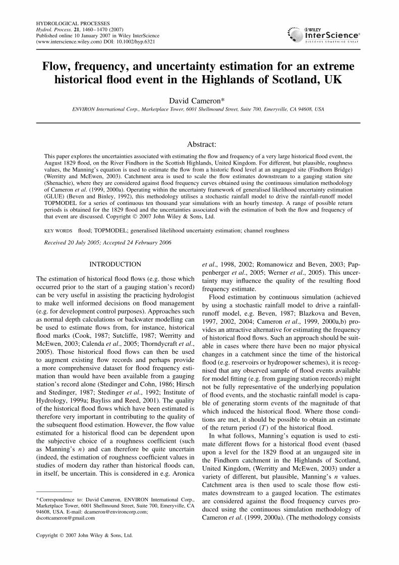
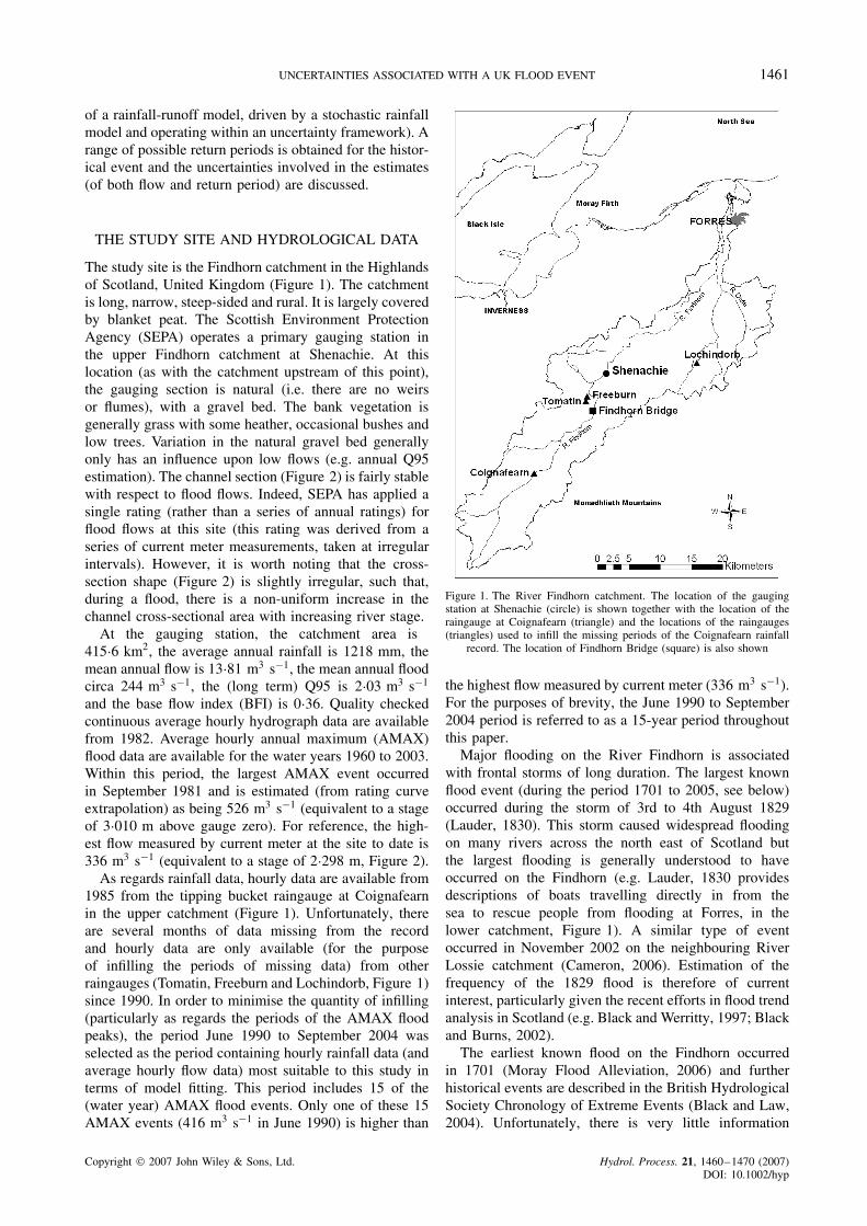
The study site is the Findhorn catchment in the Highlandsof Scotland, United Kingdom (Figure 1). The catchmentis long, narrow, steep-sided and rural. It is largely coveredby blanket peat. The Scottish Environment ProtectionAgency (SEPA) operates a primary gauging station inthe upper Findhorn catchment at Shenachie. At thislocation (as with the catchment upstream of this point),the gauging section is natural (i.e. there are no weirsor flumes), with a gravel bed. The bank vegetation isgenerally grass with some heather, occasional bushes andlow trees. Variation in the natural gravel bed generallyonly has an influence upon low flows (e.g. annual Q95estimation). The channel section (Figure 2) is fairly stablewith respect to flood flows. Indeed, SEPA has applied asingle rating (rather than a series of annual ratings) forflood flows at this site (this rating was derived from aseries of current meter measurements, taken at irregularintervals). However, it is worth noting that the cross-section shape (Figure 2) is slightly irregular, such that,during a flood, there is a non-uniform increase in thechannel cross-sectional area with increasing river stage.

At the gauging station, the catchment area is415Ð6 km2, the average annual rainfall is 1218 mm, themean annual flow is 13Ð81 m3 s�1, the mean annual floodcirca 244 m3 s�1, the (long term) Q95 is 2Ð03 m3 s�1

and the base flow index (BFI) is 0Ð36. Quality checkedcontinuous average hourly hydrograph data are availablefrom 1982. Average hourly annual maximum (AMAX)flood data are available for the water years 1960 to 2003.Within this period, the largest AMAX event occurredin September 1981 and is estimated (from rating curveextrapolation) as being 526 m3 s�1 (equivalent to a stageof 3Ð010 m above gauge zero). For reference, the high-est flow measured by current meter at the site to date is336 m3 s�1 (equivalent to a stage of 2Ð298 m, Figure 2).

As regards rainfall data, hourly data are available from1985 from the tipping bucket raingauge at Coignafearnin the upper catchment (Figure 1). Unfortunately, thereare several months of data missing from the recordand hourly data are only available (for the purposeof infilling the periods of missing data) from otherraingauges (Tomatin, Freeburn and Lochindorb, Figure 1)since 1990. In order to minimise the quantity of infilling(particularly as regards the periods of the AMAX floodpeaks), the period June 1990 to September 2004 wasselected as the period containing hourly rainfall data (andaverage hourly flow data) most suitable to this study interms of model fitting. This period includes 15 of the(water year) AMAX flood events. Only one of these 15AMAX events (416 m3 s�1 in June 1990) is higher than

Figure 1. The River Findhorn catchment. The location of the gaugingstation at Shenachie (circle) is shown together with the location of theraingauge at Coignafearn (triangle) and the locations of the raingauges(triangles) used to infill the missing periods of the Coignafearn rainfall

record. The location of Findhorn Bridge (square) is also shown

the highest flow measured by current meter (336 m3 s�1).For the purposes of brevity, the June 1990 to September2004 period is referred to as a 15-year period throughoutthis paper.

Major flooding on the River Findhorn is associatedwith frontal storms of long duration. The largest knownflood event (during the period 1701 to 2005, see below)occurred during the storm of 3rd to 4th August 1829(Lauder, 1830). This storm caused widespread floodingon many rivers across the north east of Scotland butthe largest flooding is generally understood to haveoccurred on the Findhorn (e.g. Lauder, 1830 providesdescriptions of boats travelling directly in from thesea to rescue people from flooding at Forres, in thelower catchment, Figure 1). A similar type of eventoccurred in November 2002 on the neighbouring RiverLossie catchment (Cameron, 2006). Estimation of thefrequency of the 1829 flood is therefore of currentinterest, particularly given the recent efforts in flood trendanalysis in Scotland (e.g. Black and Werritty, 1997; Blackand Burns, 2002).

The earliest known flood on the Findhorn occurredin 1701 (Moray Flood Alleviation, 2006) and furtherhistorical events are described in the British HydrologicalSociety Chronology of Extreme Events (Black and Law,2004). Unfortunately, there is very little information

Copyright 2007 John Wiley & Sons, Ltd. Hydrol. Process. 21, 1460–1470 (2007)DOI: 10.1002/hyp

1462 D. CAMERON

3.50

3.00

2.50

2.00

1.00

0 10 20 30Distance (from gauging station hut, m)

40 50 60 70

1.50

0.50

0.00

-0.50

Leve

l (m

abo

ve g

auge

zer

o) Highest gauged flow 2.298m, 336m3/s

Figure 2. Cross section of the River Findhorn at Shenachie gauging station. Levels are shown as metres above gauge zero (where gauge zero is252Ð345 metres above ordnance datum, mAOD). The level of the highest gauged flow to date is also shown

available on the ranking (in terms of magnitude) ofthese historical flood events (other than it being generallyaccepted that the 1829 flood was the largest event).This lack of information therefore precluded the typeof statistical flood frequency analysis recommended byHirsch and Stedinger (1987) and Bayliss and Reed(2001), whereby a flow threshold is applied to boththe gauged and historical floods, the floods ranked,and a plotting position formula used for return periodestimation.

It is possible to obtain a very approximate returnperiod estimate for the 1829 flood by using Gringortenplotting positions for the period 1701 to 2005 (where itis assumed that the 1829 flood is the largest flood eventin that period). The resulting return period estimate isof the order of 1 in 545 years. However, this frequencyestimate excludes an estimate of flood flow and, aswith most statistical estimates, it does not consider theprocesses which control the catchment’s storm response(e.g. the influence of antecedent soil moisture conditions).These factors may influence the quality of the frequencyestimate. These are important issues and are explicitlyconsidered in the methodology used in this paper.

ESTIMATION OF HISTORICAL FLOOD FLOWS

In a recent study, Werritty and McEwen (2003) used his-torical information (including Lauder, 1830), to identifythe level of the 1829 flood at several locations in theRiver Findhorn catchment. Of these locations, the site atFindhorn Bridge, by Tomatin, is the nearest to Shenachiegauging station (the Findhorn Bridge site is about 9 kmupstream of Shenachie, Figure 1). The present day chan-nel and floodplain at the Findhorn Bridge site are verysimilar to those at Shenachie (i.e. natural gravel bed, withgrass and heather floodplain with occasional bushes andlow trees). Examination of an 1843 map of the Tomatinarea (National Archives of Scotland, 1843) indicated thatthe floodplain vegetation at the Findhorn Bridge siteappeared to be very similar in 1843 as it is today.

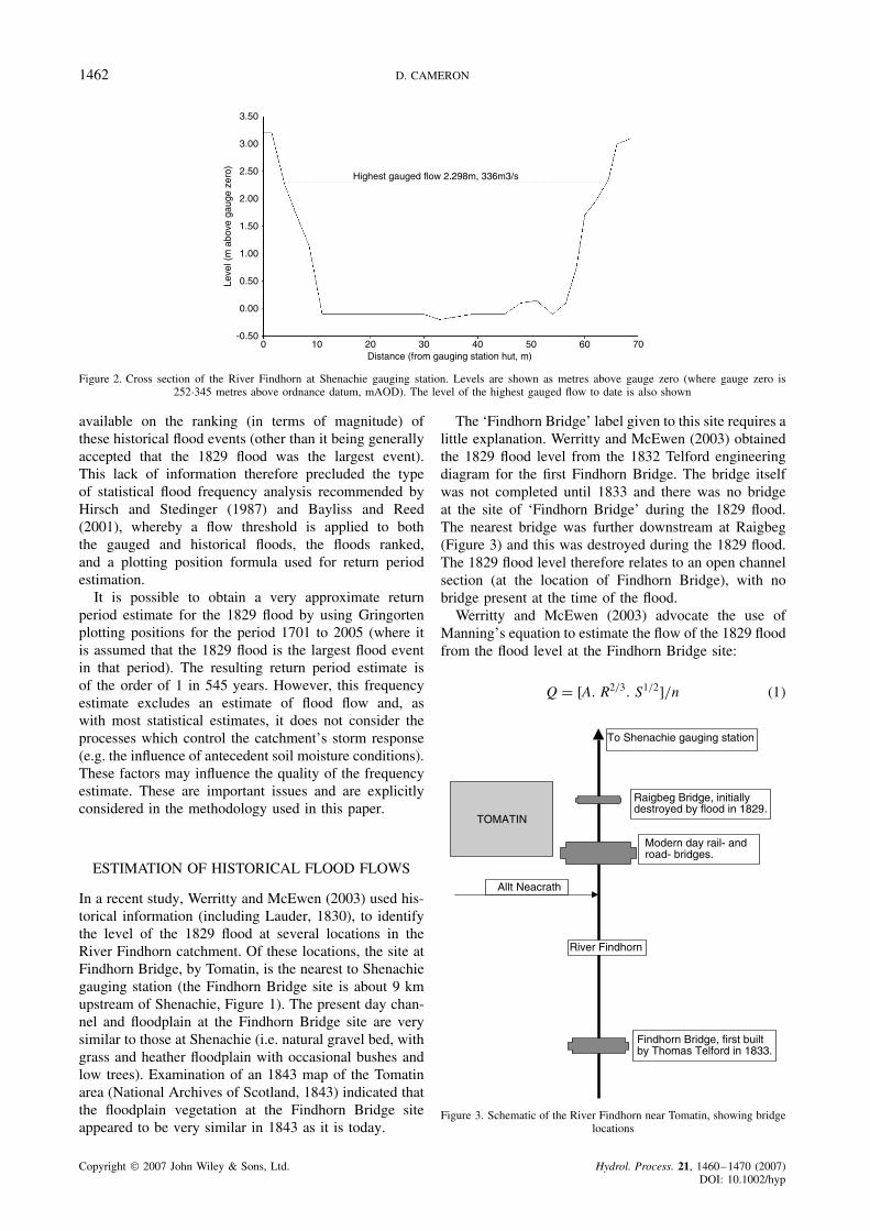
The ‘Findhorn Bridge’ label given to this site requires alittle explanation. Werritty and McEwen (2003) obtainedthe 1829 flood level from the 1832 Telford engineeringdiagram for the first Findhorn Bridge. The bridge itselfwas not completed until 1833 and there was no bridgeat the site of ‘Findhorn Bridge’ during the 1829 flood.The nearest bridge was further downstream at Raigbeg(Figure 3) and this was destroyed during the 1829 flood.The 1829 flood level therefore relates to an open channelsection (at the location of Findhorn Bridge), with nobridge present at the time of the flood.

Werritty and McEwen (2003) advocate the use ofManning’s equation to estimate the flow of the 1829 floodfrom the flood level at the Findhorn Bridge site:

Q D [A. R2/3. S1/2]/n �1�

Findhorn Bridge, first builtby Thomas Telford in 1833.

Raigbeg Bridge, initiallydestroyed by flood in 1829.

River Findhorn

To Shenachie gauging station

Modern day rail- androad- bridges.

TOMATIN

Allt Neacrath

Figure 3. Schematic of the River Findhorn near Tomatin, showing bridgelocations



Where Q is flow, A is cross-sectional area, R is thehydraulic radius (equivalent to A/wetted perimeter), S isbed slope and n is Manning’s roughness coefficient.

Use of Manning’s equation assumes uniform flowthrough the channel cross section. Clearly, this is anidealised representation of the flow. In reality, it isperhaps more likely that the flow in the channel wouldbe varied. However, given the very limited data availablefor the estimation of the historical flood flow, it would bedifficult to proceed without making this assumption. Inaddition, recent experience within SEPA (e.g. Cameronet al., 2004) has suggested that Manning’s equation canbe used (with care) to adequately estimate flood flows inrivers in the north east of Scotland.

Werritty and McEwen (2003) use values of A �322 m2�,and R (1Ð62 m) obtained from the Telford engineeringdiagram (note that, as this diagram was drawn only3 years after the 1829 flood, these are the best avail-able estimates of these values and they are also usedin this study). They adopt an S value (of 0Ð0041 m/m)obtained by field survey under present day conditions. Inthe absence of any other information describing S (histor-ically or for the present day), the S value of 0Ð0041 m/mis also used in this study (thus it is assumed that thepresent day value of S is also representative of that valuein 1829. It is acknowledged that S could have changedsince 1829. However, it is intended that the wide rangeof flows estimated under this study’s Case 2, see belowand the section “Results and Discussion”, encapsulatesother possible ranges of flows, appropriate to the Find-horn Bridge site, which might have been calculated fromdifferent combinations of S and n).

The estimation of n is thus very important as this valuewill have a large influence upon the estimate of the floodflow, Q. Two possible approaches to the estimation of nare therefore adopted in this study:

1. Case 1. The present day channel and floodplain char-acteristics at Findhorn Bridge are very similar to thoseat Shenachie (see above). If it is assumed that thosecharacteristics are generally the same today as theywere in 1829, then it is possible to use the availablehigh flow gaugings at Shenachie to back-calculate n(at Shenachie), and then directly transfer that estimateof n to Findhorn Bridge.

The stage (h) and rated flow (Qrat, as obtained fromthe station’s rating equation) associated with each highflow gauging at Shenachie is listed in Table I. Therated flows are shown in preference to the actualmeasured flows in order to make some allowance formeasurement error and maintain a consistent stage-flow relationship over the range of high flow gaugings.This dataset includes flows which overtopped the banksof the channel, but were still contained within thegauged section.

At each value of h, Qrat was used to calibrate Man-ning’s n (where S is assumed to be the same as at Find-horn Bridge, 0Ð0041 m/m). From Table I, it can be seen

Table I. List of high flow gaugings used to estimate Manning’sn. The date, stage (h), and rated flow (Qrat) associated witheach gauging are shown, together with the corresponding flowsestimated using Manning’s equation (Qn, following estimation of

Manning’s n from Qrat, see accompanying text)

Date h(m)a Qratb

(m3 s�1)Manning’s

nQn �m3 s�1�

30 Oct 1986 1Ð210 112 0Ð039 11214 Nov 1978 1Ð226 115 0Ð039 11509 Nov 1998 1Ð270 122 0Ð039 12114 Jan 1981 1Ð287 125 0Ð039 12414 Nov 1978 1Ð465 156 0Ð038 15730 Oct 1986 1Ð494 161 0Ð038 16230 Oct 1986 1Ð565 175 0Ð038 17514 Nov 1978 1Ð575 177 0Ð038 17708 Mar 1994 1Ð680 197 0Ð038 19725 Oct 1984 1Ð723 206 0Ð038 20508 Mar 1994 1Ð732 208 0Ð038 20625 Oct 1984 1Ð812 225 0Ð037 22716 Aug 1990 1Ð924 249 0Ð037 24916 Aug 1990 2Ð289 334 0Ð036 33830 Nov 1999 2Ð298 336 0Ð036 341

a Above gauge zero (where gauge zero is 252Ð345 metres above ordnancedatum, mAOD, Newlyn, United Kingdom).b Where Qrat D 90Ð4064 �h � 0Ð069�1Ð6375.

that the flows estimated using Manning’s equation (Qn)are an acceptable fit to Qrat. It is perhaps also worthnoting that, while many of the current meter gaug-ings were made during the winter months (Table I),two of the three highest gaugings were made in sum-mer (August 1990). Indeed, the higher of these twogaugings (334 m3 s�1) shares the same n value (0Ð036)as that estimated for the highest gauging (336 m3 s�1

in November 1999). It can therefore be assumed thatsummer vegetation does not significantly affect theestimation of n in this part of the Findhorn catchment.

From Table I, it can also be seen that there are steppeddecreases in the values of Manning’s n with increasedvalues of h (e.g. between h of 1Ð210 m and 1Ð287 m,n is estimated as having a value of 0Ð039, but at h ofbetween 1Ð465 m and 1Ð732, n is estimated as having avalue of 0Ð038). This finding can perhaps be explainedby the irregularity of the shape of the channel crosssection (i.e. there is a non-uniform increase in thechannel cross-sectional area with depth, see Figure 2).

The information in Table I suggests that each ‘step’results in a decrease in Manning’s n of about 0Ð001.Further investigation of the Shenachie cross sectionsuggested that there was only one further ‘step’ fromthe top of the (high flow gauged) range (associated withan n value of 0Ð036, Table I) to the top of the gaugingsection itself (this occurs at a stage of approximately3 m above gauge zero). On this basis, a Manning’s nvalue of 0Ð035 was estimated as being appropriate toflood flows through the Shenachie gauging section. Inthe absence of any objective evidence to support analternative value, this n value was used at FindhornBridge, yielding an estimate of Q of 813 m3 s�1 forthe 1829 flood.


1464 D. CAMERON

2. Case 2. If it is assumed that there is insufficientinformation to identify a single value for n, then arange of n values, which are appropriate to FindhornBridge, could be adopted. However, identifying a suit-able range is not simple. For example, for ‘MountainStreams’ with ‘bottom: gravels, cobbles and few boul-ders’ (perhaps an appropriate category for the Find-horn), Chow (1959) suggests a range of 0Ð030 to 0Ð050.However, Werritty and McEwen (2003) suggest an nvalue of 0Ð060 for Findhorn Bridge (this value beinga subjective choice based upon experience and a fieldstudy conducted in a bedrock gorge on the River Divie,a tributary of the River Findhorn some distance down-stream of Shenachie). On the basis of this information,a range of n values of 0Ð030 to 0Ð060 is assumed tobe plausible for the Findhorn Bridge and is investi-gated in this study. With S, R and A values set as perWerritty and McEwen (2003), this range yields esti-mates of Q over the range 474 m3 s�1 to 948 m3 s�1

(Table II).

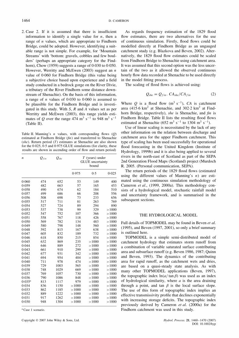
Table II. Manning’s n values, with corresponding flows (Q)estimated at Findhorn Bridge (fin) and transferred to Shenachie(she). Return period (T) estimates at Shenachie are also shownfor the 0Ð025, 0Ð5 and 0Ð975 GLUE simulations (for clarity, theseresults are shown in ascending order of flow and return period)

n Qfin Qshe T (years) underGLUE uncertainty

bound

0Ð975 0Ð5 0Ð025

0Ð060 474 652 53 149 4000Ð059 482 663 57 165 4530Ð058 490 674 62 184 5100Ð057 499 686 66 208 5560Ð056 508 698 73 233 6560Ð055 517 711 81 263 7690Ð054 527 724 89 294 8900Ð053 537 738 99 329 >10000Ð052 547 752 107 366 >10000Ð051 558 767 118 426 >10000Ð050 569 782 134 483 >10000Ð049 580 798 148 560 >10000Ð048 592 815 167 638 >10000Ð047 605 832 189 732 >10000Ð046 618 850 215 854 >10000Ð045 632 869 235 >1000 >10000Ð044 646 889 272 >1000 >10000Ð043 661 910 299 >1000 >10000Ð042 677 931 342 >1000 >10000Ð041 694 954 404 >1000 >10000Ð040 711 978 474 >1000 >10000Ð039 729 1003 565 >1000 >10000Ð038 748 1029 669 >1000 >10000Ð037 769 1057 730 >1000 >10000Ð036 790 1086 848 >1000 >10000Ð035a 813 1117 979 >1000 >10000Ð034 836 1150 >1000 >1000 >10000Ð033 862 1185 >1000 >1000 >10000Ð032 889 1222 >1000 >1000 >10000Ð031 917 1262 >1000 >1000 >10000Ð030 948 1304 >1000 >1000 >1000

a Case 1 scenario.

As regards frequency estimation of the 1829 floodflow estimates, there are two alternatives for the useof continuous simulation. Firstly, flood flows could bemodelled directly at Findhorn Bridge as an ungaugedcatchment study (e.g. Blazkova and Beven, 2002). Alter-natively, the 1829 flood flow estimates could be scaledfrom Findhorn Bridge to Shenachie using catchment area.It was assumed that this second option was the less uncer-tain of the two as it allowed the observed continuoushourly flow data recorded at Shenachie to be used directlyin the model fitting process.

The scaling of flood flows is achieved using:

Qshe D Qfin. CAshe/CAfin �2�

Where Q is a flood flow (m3 s�1), CA is catchmentarea (415Ð6 km2 at Shenachie, and 302Ð2 km2 at Find-horn Bridge, respectively), she is Shenachie, and fin isFindhorn Bridge. Table II lists the resulting flood flowsestimated at Shenachie (652 m3 s�1 to 1304 m3 s�1).

Use of linear scaling is necessitated by the lack of anyother information on the relation between discharge andcatchment area for the upper Findhorn catchment. Thistype of scaling has been used successfully for operationalflood forecasting in the United Kingdom (Institute ofHydrology, 1999b) and it is also being applied to severalrivers in the north-east of Scotland as part of the SEPA2nd Generation Flood Maps (Scotland) project (MurdochR. 2005. (Personal communication, SEPA).

The return periods of the 1829 flood flows (estimatedusing the different values of Manning’s n) are esti-mated using the continuous simulation methodology ofCameron et al., (1999, 2000a). This methodology con-sists of a hydrological model, stochastic rainfall modeland uncertainty framework, and is summarised in thesubsequent sections.

THE HYDROLOGICAL MODEL

Full details of TOPMODEL may be found in Beven et al.(1995), and Beven (1997, 2001), so only a brief summaryis outlined here.

TOPMODEL is a simple semi-distributed model ofcatchment hydrology that estimates storm runoff froma combination of variable saturated surface contributingarea and subsurface runoff (e.g. Beven 1986, 1987; Quinnand Beven, 1993). The dynamics of the contributingarea for rapid runoff, as the catchment wets and dries,are based on a quasi-steady state analysis. As withmany other TOPMODEL applications (Beven, 1997),the topographic index ln�a/ tan ˇ) was used as an indexof hydrological similarity, where a is the area drainingthrough a point, and tan ˇ is the local surface slope.The use of this form of topographic index implies aneffective transmissivity profile that declines exponentiallywith increasing storage deficits. The topographic indexpreviously derived by Cameron et al. (2000a) for theFindhorn catchment was used in this study.



Evapotranspiration losses in TOPMODEL are con-trolled by potential evapotranspiration (PET) and storagein the root zone with the parameter SRMAX (effec-tive available water capacity at the root zone). The PETestimation routine uses the same seasonal sine curve asBeven (1986, 1987) and Blazkova and Beven (1997) witha single mean hourly PET parameter. In the absence ofany readily available PET data, recourse was made toestimating PET from the observed rainfall and runoff dataavailable for the catchment (yielding a PET parametervalue of 0Ð02466 mm hr�1).

This version of TOPMODEL uses the same linearflow routing routine as that of Blazkova and Beven(1997). In this application, because of the steepness of thecatchment, and the corresponding observed velocities atthe Shenachie gauging station, a wave speed of 2 m s�1

was used.TOPMODEL (often driven by a stochastic rainfall

model) has successfully been used for flood estima-tion in many continuous simulation studies on bothgauged (Beven 1986, 1987; Blazkova and Beven, 1997,Cameron et al., 1999, 2000a-b; 2004; Cameron, 2006)and ungauged catchments (Blazkova and Beven, 2002).Cameron et al. (2000a) describe an earlier application ofTOPMODEL to the Findhorn catchment (where TOP-MODEL was run with both observed rainfall data andrainfall data simulated using a stochastic rainfall model).

THE STOCHASTIC RAINFALL MODEL

A stochastic rainfall model, similar to the one detailedin Cameron et al. (1999); (see also Cameron et al.,2000a,b,c; Cameron, 2006), was developed for the Find-horn catchment.

The stochastic rainfall model is based upon the avail-able observed hourly rainfall data and generates ran-dom rainstorms via a Monte Carlo sampling procedure(Cameron et al., 1999, for a full description of this typeof model, its operation and the model fitting procedureused). The model characterises a storm in terms of amean storm intensity, duration, inter-event arrival time,and storm profile. A rainstorm is defined as any eventwith a minimum intensity of 0Ð1 mm at an hour, witha minimum duration of 1 h and a minimum inter-eventarrival time of 1 h. This definition accounts for all of therainfall data in the observed series.

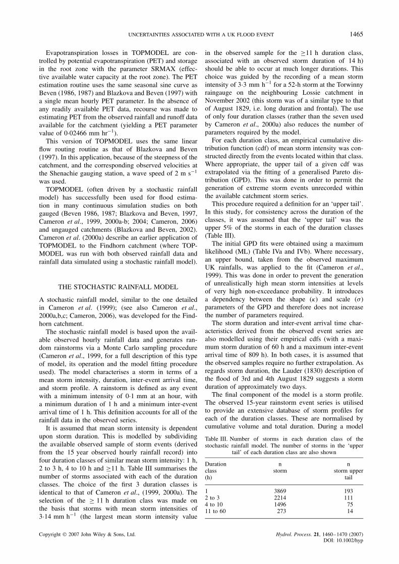
It is assumed that mean storm intensity is dependentupon storm duration. This is modelled by subdividingthe available observed sample of storm events (derivedfrom the 15 year observed hourly rainfall record) intofour duration classes of similar mean storm intensity: 1 h,2 to 3 h, 4 to 10 h and ½11 h. Table III summarises thenumber of storms associated with each of the durationclasses. The choice of the first 3 duration classes isidentical to that of Cameron et al., (1999, 2000a). Theselection of the ½ 11 h duration class was made onthe basis that storms with mean storm intensities of3Ð14 mm h�1 (the largest mean storm intensity value

in the observed sample for the ½11 h duration class,associated with an observed storm duration of 14 h)should be able to occur at much longer durations. Thischoice was guided by the recording of a mean stormintensity of 3Ð3 mm h�1 for a 52-h storm at the Torwinnyraingauge on the neighbouring Lossie catchment inNovember 2002 (this storm was of a similar type to thatof August 1829, i.e. long duration and frontal). The useof only four duration classes (rather than the seven usedby Cameron et al., 2000a) also reduces the number ofparameters required by the model.

For each duration class, an empirical cumulative dis-tribution function (cdf) of mean storm intensity was con-structed directly from the events located within that class.Where appropriate, the upper tail of a given cdf wasextrapolated via the fitting of a generalised Pareto dis-tribution (GPD). This was done in order to permit thegeneration of extreme storm events unrecorded withinthe available catchment storm series.

This procedure required a definition for an ‘upper tail’.In this study, for consistency across the duration of theclasses, it was assumed that the ‘upper tail’ was theupper 5% of the storms in each of the duration classes(Table III).

The initial GPD fits were obtained using a maximumlikelihood (ML) (Table IVa and IVb). Where necessary,an upper bound, taken from the observed maximumUK rainfalls, was applied to the fit (Cameron et al.,1999). This was done in order to prevent the generationof unrealistically high mean storm intensities at levelsof very high non-exceedance probability. It introducesa dependency between the shape (�) and scale (�)parameters of the GPD and therefore does not increasethe number of parameters required.

The storm duration and inter-event arrival time char-acteristics derived from the observed event series arealso modelled using their empirical cdfs (with a maxi-mum storm duration of 60 h and a maximum inter-eventarrival time of 809 h). In both cases, it is assumed thatthe observed samples require no further extrapolation. Asregards storm duration, the Lauder (1830) description ofthe flood of 3rd and 4th August 1829 suggests a stormduration of approximately two days.

The final component of the model is a storm profile.The observed 15-year rainstorm event series is utilisedto provide an extensive database of storm profiles foreach of the duration classes. These are normalised bycumulative volume and total duration. During a model

Table III. Number of storms in each duration class of thestochastic rainfall model. The number of storms in the ‘upper

tail’ of each duration class are also shown

Durationclass(h)

nstorm

nstorm upper

tail

1 3869 1932 to 3 2214 1114 to 10 1496 7511 to 60 273 14


1466 D. CAMERON

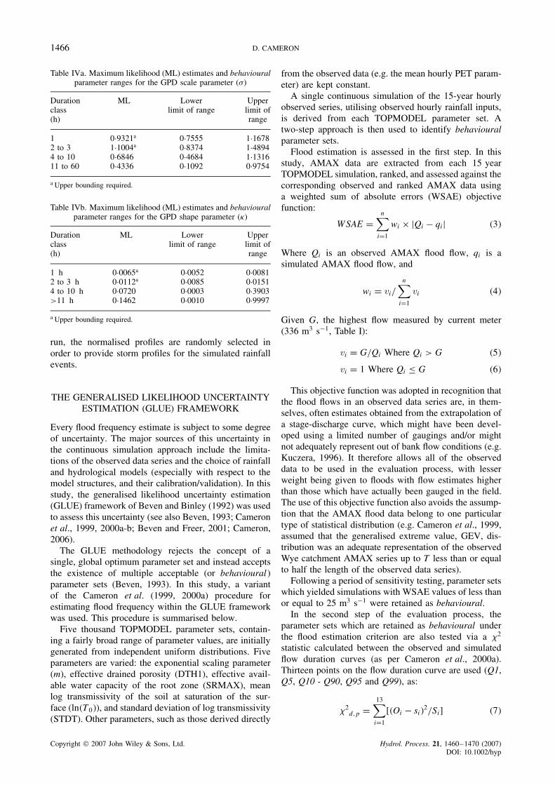
Table IVa. Maximum likelihood (ML) estimates and behaviouralparameter ranges for the GPD scale parameter (�)

Durationclass(h)

ML Lowerlimit of range

Upperlimit ofrange

1 0Ð9321a 0Ð7555 1Ð16782 to 3 1Ð1004a 0Ð8374 1Ð48944 to 10 0Ð6846 0Ð4684 1Ð131611 to 60 0Ð4336 0Ð1092 0Ð9754

a Upper bounding required.

Table IVb. Maximum likelihood (ML) estimates and behaviouralparameter ranges for the GPD shape parameter (�)

Durationclass(h)

ML Lowerlimit of range

Upperlimit ofrange

1 h 0Ð0065a 0Ð0052 0Ð00812 to 3 h 0Ð0112a 0Ð0085 0Ð01514 to 10 h 0Ð0720 0Ð0003 0Ð3903>11 h 0Ð1462 0Ð0010 0Ð9997

a Upper bounding required.

run, the normalised profiles are randomly selected inorder to provide storm profiles for the simulated rainfallevents.

THE GENERALISED LIKELIHOOD UNCERTAINTYESTIMATION (GLUE) FRAMEWORK

Every flood frequency estimate is subject to some degreeof uncertainty. The major sources of this uncertainty inthe continuous simulation approach include the limita-tions of the observed data series and the choice of rainfalland hydrological models (especially with respect to themodel structures, and their calibration/validation). In thisstudy, the generalised likelihood uncertainty estimation(GLUE) framework of Beven and Binley (1992) was usedto assess this uncertainty (see also Beven, 1993; Cameronet al., 1999, 2000a-b; Beven and Freer, 2001; Cameron,2006).

The GLUE methodology rejects the concept of asingle, global optimum parameter set and instead acceptsthe existence of multiple acceptable (or behavioural )parameter sets (Beven, 1993). In this study, a variantof the Cameron et al. (1999, 2000a) procedure forestimating flood frequency within the GLUE frameworkwas used. This procedure is summarised below.

Five thousand TOPMODEL parameter sets, contain-ing a fairly broad range of parameter values, are initiallygenerated from independent uniform distributions. Fiveparameters are varied: the exponential scaling parameter(m), effective drained porosity (DTH1), effective avail-able water capacity of the root zone (SRMAX), meanlog transmissivity of the soil at saturation of the sur-face (ln�T0�), and standard deviation of log transmissivity(STDT). Other parameters, such as those derived directly

from the observed data (e.g. the mean hourly PET param-eter) are kept constant.

A single continuous simulation of the 15-year hourlyobserved series, utilising observed hourly rainfall inputs,is derived from each TOPMODEL parameter set. Atwo-step approach is then used to identify behaviouralparameter sets.

Flood estimation is assessed in the first step. In thisstudy, AMAX data are extracted from each 15 yearTOPMODEL simulation, ranked, and assessed against thecorresponding observed and ranked AMAX data usinga weighted sum of absolute errors (WSAE) objectivefunction:

WSAE Dn∑

iD1

wi ð jQi � qij �3�

Where Qi is an observed AMAX flood flow, qi is asimulated AMAX flood flow, and

wi D vi/n∑

iD1

vi �4�

Given G, the highest flow measured by current meter(336 m3 s�1, Table I):

vi D G/Qi Where Qi > G �5�

vi D 1 Where Qi � G �6�

This objective function was adopted in recognition thatthe flood flows in an observed data series are, in them-selves, often estimates obtained from the extrapolation ofa stage-discharge curve, which might have been devel-oped using a limited number of gaugings and/or mightnot adequately represent out of bank flow conditions (e.g.Kuczera, 1996). It therefore allows all of the observeddata to be used in the evaluation process, with lesserweight being given to floods with flow estimates higherthan those which have actually been gauged in the field.The use of this objective function also avoids the assump-tion that the AMAX flood data belong to one particulartype of statistical distribution (e.g. Cameron et al., 1999,assumed that the generalised extreme value, GEV, dis-tribution was an adequate representation of the observedWye catchment AMAX series up to T less than or equalto half the length of the observed data series).

Following a period of sensitivity testing, parameter setswhich yielded simulations with WSAE values of less thanor equal to 25 m3 s�1 were retained as behavioural.

In the second step of the evaluation process, theparameter sets which are retained as behavioural underthe flood estimation criterion are also tested via a �2

statistic calculated between the observed and simulatedflow duration curves (as per Cameron et al., 2000a).Thirteen points on the flow duration curve are used (Q1,Q5, Q10 - Q90, Q95 and Q99), as:

�2d,p D

13∑

iD1

[�Oi � si�2/Si] �7�



Where d is twelve degrees of freedom, p D 0Ð9,Oi is the observed percentage time spent beneath agiven flow value, and Si is the simulated percentagetime spent beneath a given flow value. This yields arejection threshold of 18Ð5. Parameter sets which providesimulations which meet or fall below this threshold areretained as behavioural.

The behavioural area of the parameter space is thenresampled until 1000 behavioural TOPMODEL param-eter sets are obtained (Table V contains the parameterranges associated with these behavioural parameter sets).

In order to provide flood frequency estimates beyondthe upper return period limit of the observed series,the stochastic rainfall generator is coupled with TOP-MODEL. This requires the estimation of the rainfallmodel’s GPD parameters prior to the runs with TOP-MODEL and this is also achieved within the GLUEframework.

Five thousand GPD parameter sets are initially gen-erated for each cdf upper tail requiring extrapolation.For the cases where the ML estimate of the GPD fitrequires an upper bound (see section “The StochasticRainfall Model”), � is sampled from a uniform distri-bution. Upper bounding is assumed and � calculated (seesection “The Stochastic Rainfall Model”). For the othercdf upper tails, both � and � are independently sampledfrom uniform distributions, and a parameter set is rejectedas non-behavioural if the upper bound is exceeded. Forthese latter upper tails only, this more explicit form ofbounding produces superior GPD fits to the data in com-parison with those obtained through the first procedure.

The GPD parameter sets retained by each procedureare also evaluated in terms of providing a reasonablegoodness-of-fit to the appropriate cdf upper tail. This iscalculated using the log likelihood measure, l��, as:

l��du Dnp∑

iD1

� log � C �1/� � 1�

. log[1 � � . �xi � u�/�] �8�

Where du is the particular cdf upper tail, � is a shapeparameter, u is a location parameter (or threshold), xi isan event in the upper tail, np is the number of events inthat tail and xi � u is an exceedance.

Rejection of the non-behavioural GPD parameter setsis achieved as follows. On a cdf upper tail basis, thedeviance of a given value of l�� from the original ML

Table V. Parameter ranges of the 1000 behavioural TOPMODELparameter sets

Parameter Lowerlimit of range

Upperlimit ofrange

m (m) 0Ð0071 0Ð0091SRMAX (m) 0Ð0214 0Ð4936T0 (log) 0Ð5624 6Ð0804STDT (log) 4Ð6366 9Ð9756DTH1 0Ð0184 0Ð9422

estimate (see section “The Stochastic Rainfall Model”) iscalculated and compared with a threshold deviance (TD),as:

Dpa � TD �9�

Where D is the deviance calculated between the MLestimate, l��, and the value of l�� for a given parameterset (pa), as:

Dpa D 2[l�� l��pa] �10�

and TD is a threshold deviance of 4Ð61 obtained from the�2 distribution at 2 degrees of freedom (for the GPD) anda probability level of p D 0Ð9. The TD is consistent foreach upper tail.

The behavioural area of the parameter space is thenresampled until 1000 behavioural rainfall parameter setsare obtained. Table IVa and IVb contain the behaviouralranges of � and �, respectively.

One thousand behavioural TOPMODEL and rainfallparameter sets (chosen randomly) are then used to pro-duce a 1000-element series of ten thousand year hourlyflow simulations. (The ten thousand year simulationlength is adopted in order to minimise the effects ofthe random sampling process used in the rainfall model,in the estimation of floods of return periods of up to1 in 1000 years. In this study, it is assumed that 1in 1000 years is the upper limit for meaningful returnperiod estimates of the 1829 flood flows. Where flowsare estimated to have even higher return periods, theseare simply listed as >1 in 1000 years).

These parameter sets are used to calculate the likeli-hood weighted uncertainty bounds for the ten thousandyear flood frequency simulations. This requires the use ofa combined measure (CM), which assumes equal weight-ings between the rainfall and TOPMODEL parametersets:

CM D 1/WSAEs . 1/nd .nd∑

iD1

[Ls��i] �11�

Where s denotes that the objective function has beenrescaled (such that all of the objective functions sharea common scale), nd is the number of cdfs requiringextrapolation (four), and L�� is the exponential of l��.

The CM likelihood weights are rescaled over all of thebehavioural simulations in order to produce a cumulativesum of 1Ð0. A cdf of discharge estimates is constructedfor each AMAX peak using the rescaled weights. Linearinterpolation is used to extract the discharge estimateappropriate to cumulative likelihoods of 0Ð025, 0Ð5, and0Ð975. This allows 95% uncertainty bounds, in additionto a median simulation, to be derived (see also Blazkovaand Beven, 2002, 2004; Cameron et al., 1999, 2000a-b;Cameron, 2006).

RESULTS AND DISCUSSION

Before discussing frequency estimation for the 1829flood, it is useful to consider the performance of the


1468 D. CAMERON

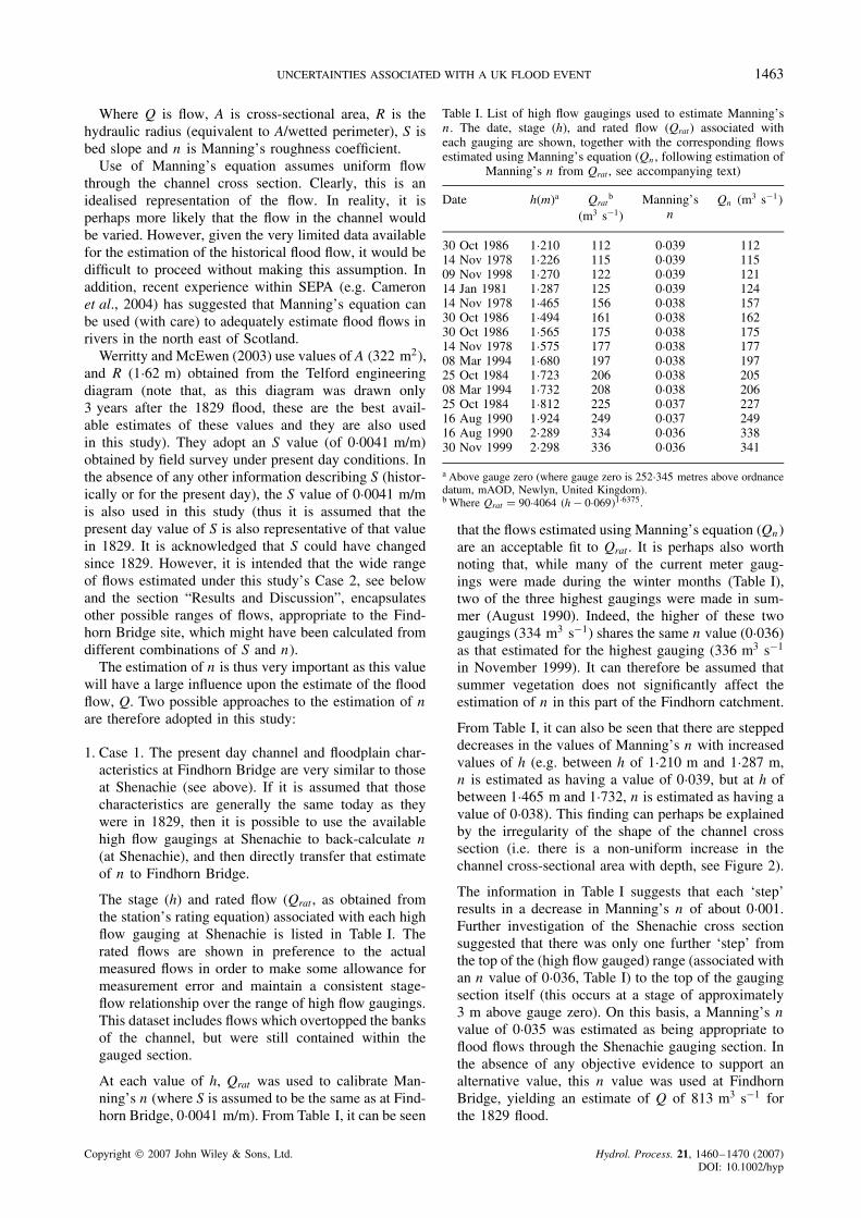
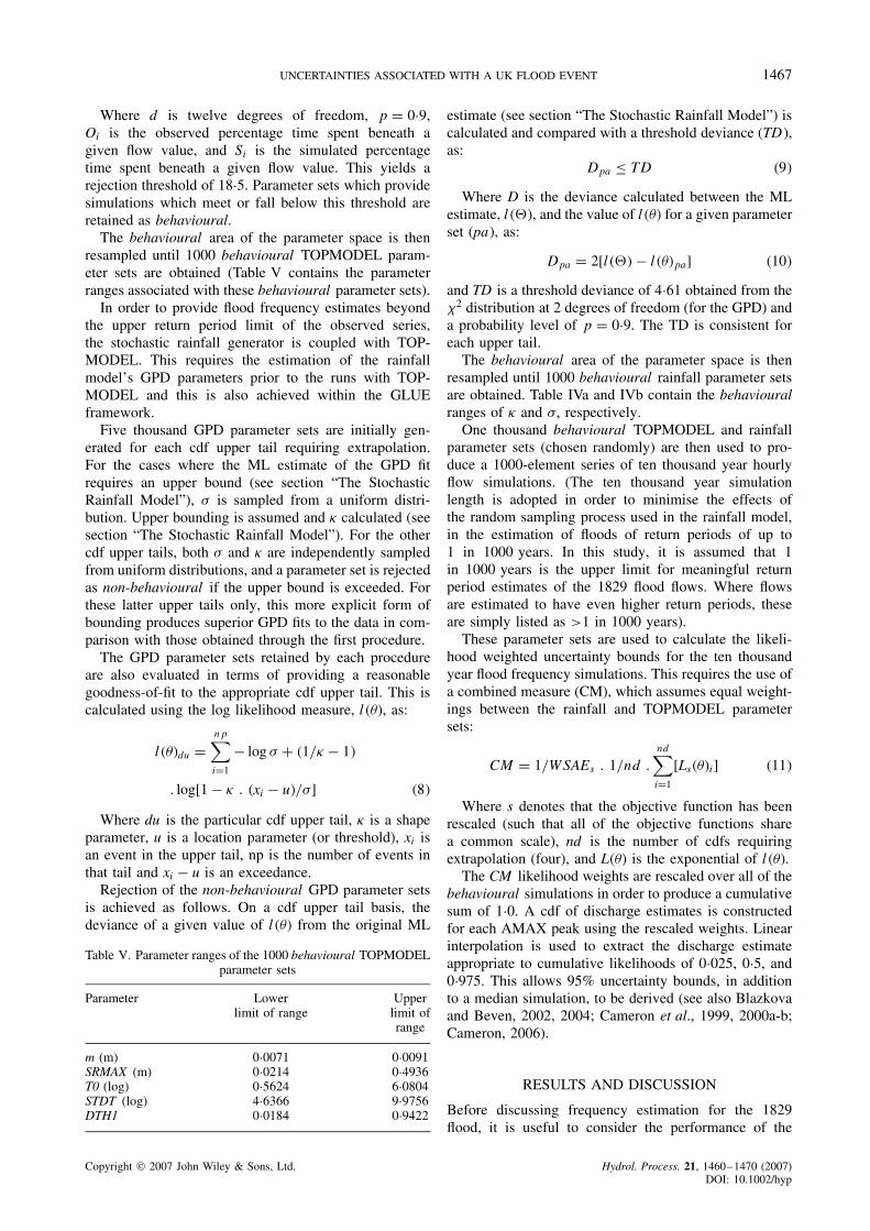
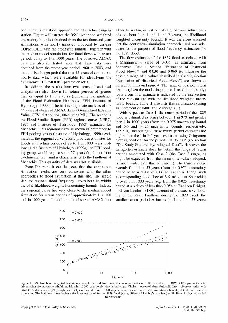
continuous simulation approach for Shenachie gaugingstation. Figure 4 illustrates the 95% likelihood weighteduncertainty bounds (obtained from the ten thousand yearsimulations with hourly timestep produced by drivingTOPMODEL with the stochastic rainfall), together withthe median model simulation, for flood flows with returnperiods of up to 1 in 1000 years. The observed AMAXdata are also illustrated (note that these data wereobtained from the water year period 1960 to 2003, andthat this is a longer period than the 15 years of continuoushourly data which were available for identifying thebehavioural TOPMODEL parameter sets).

In addition, the results from two forms of statisticalanalysis are also shown for return periods of greaterthan or equal to 1 in 2 years (following the guidanceof the Flood Estimation Handbook, FEH, Institute ofHydrology, 1999a). The first is single site analysis of the44 years of observed AMAX data (a Generalised ExtremeValue, GEV, distribution, fitted using ML). The second isthe Flood Studies Report (FSR) regional curve (NERC,1975 and Institute of Hydrology, 1983) estimated forShenachie. This regional curve is shown in preference toFEH pooling group (Institute of Hydrology, 1999a) esti-mates as the regional curve readily provides estimates forfloods with return periods of up to 1 in 1000 years. Fol-lowing the Institute of Hydrology (1999a), an FEH pool-ing group would require some 5T years flood data fromcatchments with similar characteristics to the Findhorn atShenachie. This quantity of data was not available.

From Figure 4, it can be seen that the continuoussimulation results are very consistent with the otherapproaches to flood estimation at this site. The singlesite and regional flood frequency curves both lie withinthe 95% likelihood weighted uncertainty bounds. Indeed,the regional curve lies very close to the median modelsimulation for return periods of approximately 1 in 100to 1 in 1000 years. In addition, the observed AMAX data

either lie within, or just out of (e.g. between return peri-ods of about 1 in 1 and 1 and 2 years), the likelihoodweighted uncertainty bounds. It was therefore assumedthat the continuous simulation approach used was ade-quate for the purpose of flood frequency estimation forthe 1829 flood.

The flow estimates of the 1829 flood associated witha Manning’s n value of 0Ð035 (as estimated fromShenachie, Case 1, Section “Estimation of HistoricalFlood Flows”) and 0Ð030 and 0Ð060 (to illustrate thepossible range of n values described in Case 2, Section“Estimation of Historical Flood Flows”) are shown ashorizontal lines on Figure 4. The range of possible returnperiods (given the modelling approach used in this study)for a given flow estimate is indicated by the intersectionof the relevant line with the likelihood weighted uncer-tainty bounds. Table II also lists this information (usingan increment of 0Ð001 for Manning’s n).

With respect to Case 1, the return period of the 1829flood is estimated as being between 1 in 979 and greaterthan 1 in 1000 years (from the 0Ð975 uncertainty boundand 0Ð5 and 0Ð025 uncertainty bounds, respectively,Table II). Interestingly, these return period estimates arehigher than the 1 in 545 years estimated using Gringortenplotting positions for the period 1701 to 2005 (see section“The Study Site and Hydrological Data”). However, theGringorten estimate does lie within the range of returnperiods associated with Case 2 (the Case 2 range, asmight be expected from the range of n values adopted,is much wider than that of Case 1). The Case 2 rangeextends from 1 in 53 years (from the 0Ð975 uncertaintybound at an n value of 0Ð06 at Findhorn Bridge, witha corresponding flood flow of 607 m3 s�1 at Shenachie)to over 1 in 1000 years (e.g. from the 0Ð025 uncertaintybound at n values of less than 0Ð054 at Findhorn Bridge).

Given Lauder’s (1830) account of the excessive flood-ing of the River Findhorn during the 1829 event, thesmaller return period estimates (such as 1 in 53 years)

1400

1200

n = 0.030

n = 0.035

n = 0.060

1000

800

600

400

200

01 10 100 1000

T (years)

Q (

m3/

s)

Figure 4. 95% likelihood weighted uncertainty bounds derived from annual maximum peaks of 1000 behavioural TOPMODEL parameter sets,driven using the stochastic rainfall model, with 10 000 year hourly simulation length. Circles—observed data; dark solid line—observed series withfitted GEV distribution (ML; single site analysis); dash-dot line—FSR region curve; dashed lines—95% uncertainty bounds; dotted line—mediansimulation. The horizontal lines indicate the flows estimated for the 1829 flood (using different Manning’s n values) at Findhorn Bridge and scaled

to Shenachie



are perhaps unrealistic conceptually. Interestingly, thereturn period estimates of greater than 1 in 1000 years(on the 0Ð975 uncertainty bound) estimated from flowsassociated with n values of lower than about 0Ð034,seem (conceptually) very high. Assuming that the floodfrequency estimates obtained, using the continuous sim-ulation approach, are adequate, then it seems likely thatthe range of n values selected under Case 2 includes val-ues which are inappropriate for the Findhorn Bridge site.For example, if the upper limit of the range was reducedto, say, an n of 0Ð050 (from the range suggested byChow, 1959, see section “Estimation of Historical FloodFlows”), then the minimum return period for the 1829flood would be estimated as being circa 1 in 134 years.A subjective range of conceptually realistic flows at Find-horn Bridge for the 1829 flood might thus be 569 m3 s�1

to 836 m3 s�1 (with corresponding n values of 0Ð050 to0Ð034; note that this range of flows could also be gener-ated from alternative values of S and n, section “Estima-tion of Historical Flood Flows). However, without furtherinformation on the channel and floodplain characteris-tics at the Findhorn Bridge site in 1829, it is difficult toobjectively narrow the range in such a manner.

In order to put the flow estimates in the context ofrecent large floods in Scotland, Table VI lists the specificdischarges estimated for the 1829 flood on the Findhorn,together with those estimated for recent floods on theRivers Don (Aberdeenshire), Tay, and Lossie. It can beseen that even the smallest estimate of specific dischargefor the 1829 flood on the Findhorn (1Ð568 m3 s�1 km�2)is greater than twice that of the largest specific dischargeestimated for the other rivers (0Ð718 m3 s�1 km�2 for theRiver Lossie at Sheriffmills in November 2002). Thesefindings therefore emphasise the significance of the 1829Findhorn event in Scottish flood hydrology.

The results presented above highlight the uncertain-ties associated with the estimation of flood flows fromhistorical flood levels (in cases where there is only lim-ited information to suggest suitable values for roughnesscoefficients). As has also been demonstrated in studies ofpresent day floods (e.g. Aronica et al., 1998; Romanow-icz and Beven, 2003; Pappenberger et al., 2005), thisstudy has shown that the estimation of roughness coef-ficients can be quite uncertain. Furthermore, the flowestimated for a historical flood can be very sensitive tothe choice of roughness coefficient value. This choice can

also influence the frequency estimation of the historicalflood. The results also show that, given the conditionslisted in the section “Introduction”, continuous rainfall-runoff simulation can be used to estimate the frequencyof historical flood events while explicitly acknowledgingthe uncertainties associated with the estimates of thoseflood flows and their return periods.

CONCLUSIONS

This paper has explored the uncertainties associatedwith estimating the flow and frequency of a very largehistorical flood event, the August 1829 flood, on the RiverFindhorn in the Highlands of Scotland, United Kingdom.Manning’s equation was used to estimate the flow of thisevent from a historical level at an ungauged location(the site of Findhorn Bridge). The channel dimensions(including cross-sectional area, hydraulic radius and bedslope) described by Werritty and McEwen (2003) wereused. Manning’s n was estimated under two differentscenarios: Case 1 (where it was assumed that an nof 0Ð035 estimated at a downstream gauging station,Shenachie, was also applicable to Findhorn Bridge in1829) and Case 2 (where a range of n values from 0Ð030to 0Ð060 were investigated). Flow estimates were madeusing each n value in Case 1 and Case 2.

Each flow estimate was then scaled (using catchmentarea) downstream to Shenachie gauging station. Thiswas done in order to allow each flow estimate to beconsidered against the flood frequency curves obtained(at the gauging station) using the continuous simulationmethodology of Cameron et al. (1999, 2000a). Thismethodology utilises a stochastic rainfall model to drivethe rainfall-runoff model TOPMODEL for a series ofcontinuous ten thousand year simulations with hourlytimestep (in order to allow floods with return periods ofup to 1 in 1000 years to be estimated adequately). Theuncertainty in the resulting simulated annual maximumflood peaks is handled within the GLUE framework ofBeven and Binley (1992). Under Case 1, the return periodof the 1829 flood was estimated as being between 1 in979 and greater than 1 in 1000 years. Under Case 2,the corresponding range of return periods increased tobetween 1 in 53 and greater than 1 in 1000 years.

These findings indicate that the estimation of historicalflood flows (and their associated return periods, given

Table VI. Comparison of the specific discharges estimated for the 1829 flood on the River Findhorn with specific discharges estimatedfor recent large floods on other rivers in Scotland

Watercourse Site Catchmentarea

(km2)

Date of floodevent

Q(m3 s�1)

Specificdischarge

(m3 s�1 km�2)

Don (Dyce, near Aberdeen) Parkhill 1273Ð0 22/11/2002 412 0Ð323Tay Caputh 3210Ð0 17/01/1993 1878 0Ð585Lossie Sheriffmills 216Ð0 16/11/2002 155 0Ð718Findhorn Findhorn Bridge 302Ð2 04/08/1829 813a (474 to 1304)b 2Ð690a (1Ð568 to 3Ð137)b

a Case 1 scenario.b Range of estimates obtained from Case 2 scenario.


1470 D. CAMERON

the modelling approach used in this study) can bevery sensitive to the choice of roughness coefficientvalue. The results also show that, given appropriatechoices of catchment, stochastic rainfall model, rainfall-runoff model, and model fitting procedure, continuoussimulation can be used to estimate the frequency ofhistoric flood events while explicitly acknowledging theuncertainties associated with those estimates.

ACKNOWLEDGEMENTS

Thanks to Alan Werritty (University of Dundee) andLindsey McEwen (University of Gloucestershire) for dis-cussions on the 1829 flood on the Findhorn. Thanks alsoto Keith Beven (University of Lancaster) for commentsupon an early draft of this paper. The comments of threeanonymous referees contributed to the final version of thispaper. The opinions expressed in this paper are those ofthe author and do not necessarily reflect the view of theScottish Environment Protection Agency.

REFERENCES

Aronica G, Hankin B, Beven K. 1998. Uncertainty and equifinality incalibrating distributed roughness coefficients in a flood propagationmodel with limited data. Advances in Water Resources 22: 349–365.

Aronica G, Bates PD, Horritt MS. 2002. Assessing the uncertaintyin distributed modelling predictions using observed binary patterninformation within GLUE. Hydrological Processes 16: 2001–2016.

Bayliss AC, Reed DW. 2001. The Use of Historical Data in FloodFrequency Estimation, Report to MAFF . Centre for Ecology andHydrology: Wallingford.

Beven K. 1986. Hillslope runoff processes and flood frequencycharacteristics. In Hillslope Processes , Abrahams AD (ed.). Allen andUnwin: Boston; 187–202.

Beven K. 1987. Towards the use of catchment geomorphology in floodfrequency predictions. Earth Surface Processes and Landforms 12:69–82.

Beven KJ. 1993. Prophecy, reality and uncertainty in distributedhydrological modelling. Advances in Water Resources 16: 41–51.

Beven KJ (ed.). 1997. Distributed Modelling In Hydrology: Applicationsof the TOPMODEL Concepts . Wiley: Chichester.

Beven KJ. 2001. Rainfall-runoff Modelling, The Primer . Wiley:Chichester.

Beven KJ, Binley A. 1992. The future of distributed models: modelcalibration and uncertainty prediction. Hydrological Processes 6:279–298.

Beven K, Freer J. 2001. Equifinality, data assimilation, and uncertaintyestimation in mechanistic modelling of complex environmental systemsusing the GLUE methodology. Journal of Hydrology 249: 11–29.

Beven K, Lamb R, Quinn P, Romanowicz R, Freer J. 1995. TOP-MODEL. In Computer Models Of Watershed Hydrology , Singh VP(ed.). Water Resources Publications: Highlands Ranch, CO 627–668.

Black AR, Werritty A. 1997. Seasonality of flooding: a case study ofNorth Britain. Journal of Hydrology 195: 1–25.

Black AR, Burns JC. 2002. Re-assessing the flood risk in Scotland. TheScience of the Total Environment 294: 169–184.

Black AR, Law FM. 2004. Development and utilisation of a nationalweb-based chronology of hydrological events. Hydrological SciencesJournal 49: 237–246.

Blazkova S, Beven KJ. 1997. Flood frequency prediction for data limitedcatchments in the Czech Republic using a stochastic rainfall model andTOPMODEL. Journal of Hydrology 195: 256–278.

Blazkova S, Beven K. 2002. Flood frequency estimation by continuoussimulation for a catchment treated as ungauged (with uncertainty).Water Resources Research 38(8): 10Ð1029/2001WR000500.

Blazkova S, Beven K. 2004. Flood frequency estimation by continuoussimulation of subcatchment rainfalls and discharges with the aim

of improving dam safety assessment in a large basin in the CzechRepublic. Journal of Hydrology 292: 153–172.

Calenda G, Mancini CP, Volpi E. 2005. Distribution of the extreme peakfloods of the Tiber river from the XV century. Advances in WaterResources 28: 615–625.

Cameron D. 2006. An application of the UKCIP02 climate changescenarios to flood estimation by continuous simulation for a gaugedcatchment in the north east of Scotland, UK (with uncertainty). Journalof Hydrology 328: 212–226.

Cameron DS, Beven KJ, Tawn J, Naden P. 2000a. Flood frequencyestimation by continuous simulation (with likelihood based uncertaintyestimation). Hydrology and Earth System Sciences 4(1): 23–34.

Cameron DS, Beven KJ, Naden P. 2000b. Flood frequency estimationby continuous simulation under climate change (with uncertainty).Hydrology and Earth System Sciences 4(3): 393–405.

Cameron DS, Beven KJ, Tawn J. 2000c. An evaluation of three stochasticrainfall models. Journal of Hydrology 228: 130–149.

Cameron D, Murdoch R, Fraser D. 2004. Re-estimating flood flows forthe Rivers Lossie and Findhorn in Moray, Scotland. Circulation 83:17–19.

Cameron DS, Beven KJ, Tawn J, Blazkova S, Naden P. 1999. Floodfrequency estimation by continuous simulation for a gauged uplandcatchment (with uncertainty). Journal of Hydrology 219: 169–187.

Chow VT. 1959. Open Channel Hydraulics . McGraw-Hill: New York.Cook JL. 1987. Quantifying peak discharges for historical floods. Journal

of Hydrology 96: 29–40.Hirsch RM, Stedinger JR. 1987. Plotting positions for historical floods

and their precision. Water Resources Research 23: 715–727.Institute of Hydrology. 1983. Flood Studies Supplementary Report No.

14, Review of Regional Growth Curves . Institute of Hydrology:Wallingford.

Institute of Hydrology. 1999a. Flood Estimation Handbook . Institute ofHydrology: Wallingford.

Institute of Hydrology. 1999b. KW: An Extended Kinematic Wave FlowRouting Model For Real Time Use, A Guide. Institute of Hydrology:Wallingford.

Kuczera G. 1996. Correlated rating curve error in flood frequencyinference. Water Resources Research 32: 2119–2127.

Lauder TD Sir. 1830. The Great Moray Floods of 1829 , Moray Books,1998 Edition.

Moray Flood Alleviation. 2006. Forres Flood Chronology . On-line at:http://morayflooding.org/background/flooding history/forres chrono.htm.

National Archives of Scotland. 1843. Plan of Estate of Tomatin,the Property of Duncan MacBean. National Archives of Scotland:reference number RHP23995.

Natural Environment Research Council (NERC). 1975. Flood StudiesReport . Whitefriars Press: London.

Pappenberger F, Beven K, Horritt M, Blazkova S. 2005. Uncertaintyin the calibration of effective roughness parameters in HEC-RASusing inundation and downstream water level observations. Journalof Hydrology 302: 46–69.

Quinn PF, Beven KJ. 1993. Spatial and temporal predictions of soil mois-ture dynamics, runoff, variable source areas and evapotranspiration forplynlimon, mid-wales. Hydrological Processes 7: 425–448.

Romanowicz R, Beven K. 2003. Estimation of flood inundationprobabilities as conditioned on event inundation maps. Water ResourcesResearch 39: 10Ð1029/2001WR001056.

Stedinger JR, Cohn TA. 1986. Flood frequency analysis with historicaland paleoflood information. Water Resources Research 22: 785–793.

Stedinger JR, Vogel RM, Foufoula-Georgiou E. 1992. Frequency analy-sis of extreme events. In Handbook of Hydrology , Maidment DR (ed.).McGraw-Hill: New York 18Ð1–18Ð66, Chapt. 18.

Sutcliffe JV. 1987. The use of historical records in flood frequencyanalysis. Journal of Hydrology 96: 159–171.

Thorndycraft VR, Benito G, Rico M, Sopena A, Sanchez-Moya Y,Casas A. 2005. A long-term flood discharge record derived fromslackwater flood deposits of the Llobregat river, NE Spain. Journalof Hydrology 313: 16–31.

Werner M, Blazkova S, Petr J. 2005. Spatially distributed observationsin constraining inundation modelling uncertainties. HydrologicalProcesses 19: 3081–3096.

Werritty A, McEwen L. 2003. The “Muckle Spate” of 1829–Reconstruct-ion of a catastrophic flood on the river Findhorn, Scottish Highlands. InPalaeofloods, Historical Floods and Climatic Variability: Applicationsin Flood Risk Assessment , Thorndycraft VR, Benito G, Barriendos M,Llasat MC. Proceedings of the PHEFRAWorkshop: Barcelona, 16-19thOctober, 2002.


Documents

Flow, frequency, and uncertainty estimation for an extreme historical flood event in the Highlands of Scotland, UK