Flow Dimension and Anomalous Diﬀ usion Ù ã ½Ý of …xanalytica.com/links/papers/VZJ_Cello_2009.pdf · Flow Dimension and Anomalous Di ... its semilog derivative vs. time (Bourdet

www.vadosezonejournal.org · Vol. 8, No. 1, February 2009 258

I , petroleum reservoirs, geothermal

reservoirs, and waste disposal sites throughout the world are

located in fractured rock formations. Responsible management

of these resources and sites requires appropriate fi eld character-

ization studies and modeling techniques to assess the impact of

management alternatives. Th ese highly heterogeneous systems

tend to concentrate fl uid fl ow into channels of complex geom-

etry, where superposed structures of various sizes may have a

nonnegligible contribution to the overall fl ow (Bour and Davy,

1997). Traditional approaches to subsurface characterization and

modeling that assume homogeneity and space-fi lling geometry

are poorly suited to fractured rocks (Committee on Fracture

Characterization and Fluid Flow, 1996), leading to weak inter-

pretations of test data and unreliable parameter estimates.

An alternative understanding of fractured rock aquifers is

the generalized radial fl ow (GRF) model, which fi ts a param-

eter known as the fl ow dimension, n, to describe the change

in the cross-sectional area of fl ow with radial distance from the

pumped well (Barker, 1988). Where heterogeneities restrict fl ow

into erratic channels, the fl ow dimension can be less than the

spatial (Euclidean) dimension of the aquifer, a phenomenon that

has been observed at many fi eld sites (Acuna and Yortsos, 1995;

Bangoy et al., 1992; de Dreuzy and Davy, 2007). Unlike the

parameters inferred from traditional interpretations of aquifer

tests, the relationships among the fl ow dimension, aquifer het-

erogeneity, and fracture connectivity have received comparatively

little attention in the literature.

Th is study examined the connectivity, fl ow dimension, and

time scaling of diff usion for a two-dimensional aquifer whose

heterogeneity is represented by a DFN with a length distribution

following a power law of the form

( ) −= β an l l [1]

where n(l)dl is the number of faults having a length in the range

[l, l + dl], β is a density coeffi cient that controls the intensity of

fracturing in the system, and a is an exponent, typically inferred

from observations, that determines how rapidly the number of

fractures declines with length, l.Th is length law introduces long-range spatial correlations

that are consistent with the fractal nature of observed fractures.

Th e emphasis of this study was on fracture connectivity regimes

that produce the noninteger fl ow dimensions inferred from

Flow Dimension and Anomalous Diff usion of Aquifer Tests in Fracture NetworksPablo A. Cello, Douglas D. Walker, Albert J. Valocchi,* and Bruce Lo is

P. Cello and A.J. Valocchi, Civil and Environmental Engineering Dep., Univ. of Illinois, 205 N. Mathews Ave., Urbana, IL 61801; D.D. Walker, Illinois State Water Survey, 2204 Griffi th Dr., Champaign, IL 61820; B. Lo is, Rosen Center for Advanced Compu ng, Purdue Univ., West Lafaye e, IN. Received 20 Feb. 2008. *Corresponding author ([email protected]).

Vadose Zone J. 8:258–268doi:10.2136/vzj2008.0040

© Soil Science Society of America677 S. Segoe Rd. Madison, WI 53711 USA.All rights reserved. No part of this periodical may be reproduced or transmi ed in any form or by any means, electronic or mechanical, including photocopying, recording, or any informa on storage and retrieval system, without permission in wri ng from the publisher.

A : DFN, discrete fracture network; GRF, generalized radial fl ow; mvG, multivariate Gaussian.

S S

: F

Characteriza on and modeling of aquifers is par cularly challenging in fractured media, where fl ow is concentrated into channels that are poorly suited to tradi onal approaches to analysis. The generalized radial fl ow model is an alterna ve method for hydraulic test interpreta on that infers an addi onal parameter, the fl ow dimension n, to describe the fl ow geometry. This study was a Monte Carlo analysis of numerical models of aquifer tests in two-dimensional fractured media, with the objec ve of understanding the rela onships between the parameters of a discrete fracture network (DFN) with lengths distributed as a power law, the fl ow dimension, and the regime of hydraulic diff usion (e.g., Fickian or non-Fickian). The diff usion regime of each realiza on was evaluated using ⟨R2⟩ ? tk, where t is me, ⟨R2⟩ is the mean squared radius of hydraulic diff usion, and an apparent value of k = 1 indicates normal (Fickian) diff usion and k < 1 indicates anomalous (non-Fickian) diff usion. For the DFN model, the apparent fl ow dimension and exponent k depend on both the density and the power of the fracture length distribu on, and thus also on the connec vity regime of the fracture network system. Depending on the connec vity regime, the apparent fl ow dimension stabilizes to less than the Euclidean dimension and the apparent value of k < 1 indicates that hydraulic diff usion is non-Fickian. These results suggest that the fl ow dimension and the exponent k may be useful for characterizing fl ow and transport in fractured media.


aquifer tests in fractured rock aquifers. Th e study consisted of

a Monte Carlo analysis of a numerical model of an aquifer test

in a heterogeneous transmissivity fi eld, similar to Walker et al.

(2006b). For the sake of comparison, the analysis was repeated for

an aquifer whose heterogeneity follows a multivariate Gaussian

(mvG) distribution for the logarithm of transmissivity.

BackgroundA variety of models have been developed to address fl ow and

transport in fractured rock aquifers. Approaches include dual-

porosity models (Warren and Root, 1963), the multiple continua

approach (Pruess and Narasimhan, 1985), and the DFN method

(Cacas et al., 1990). Th e fi rst two models represent the fractured

system as eff ective continua, but typical applications of these

models do not describe the multiple length scales observed in

naturally fractured systems. Th e third model, the DFN, rep-

resents fractures as discrete linear features whose connectivity

and fl ow properties depend on the distribution and shape of

the features. Regardless of the conceptualization of fractures

in models, methods for characterizing and modeling fractured

media have lagged (Committee on Fracture Characterization

and Fluid Flow, 1996).

Th e interpretation of aquifer tests for the characterization

of fractured rock aquifers requires an approach that addresses

the complex geometry of fl ow. Barker (1988) introduced n to

generalize the traditional interpretation model of radial fl ow to a

pumping well during an aquifer test. In the resulting GRF model,

n describes how the cross-sectional area of the fl ow changes with

radial distance from the pumped well:

( )( )

− −π=

Γ

/23 12

2

nn nA r b r

n [2]

where A is the area, r is the radial distance, b is the thickness of the

aquifer, and Γ is the gamma function. Th e fl ow dimension can be

inferred from a constant-rate aquifer test in a nonleaky, infi nite-

acting aquifer using the log–log diagnostic plot of Bourdet et al.

(1983). For such tests, the late-time slope, ν, of the log–log plot

of the derivative of drawdown is related to the apparent fl ow

dimension by

( ) ( )= − ν* 2 2n t t [3]

where

( )( )

⎡ ⎤⎛ ⎞⎟⎜⎢ ⎥ν = ⎟⎜ ⎟⎜⎢ ⎥⎝ ⎠⎣ ⎦

d dlog

d log d ln

ht

t t [4]

(Barker, 1988; Mishra et al., 1991). For a constant-rate aquifer

test in a homogeneous, infi nite, two-dimensional domain, n = 2

by defi nition, which requires the late-time slope of the drawdown

derivative to be ν(t) = 0. Th e apparent fl ow dimension is a func-

tion of time because heterogeneities can cause the apparent fl ow

dimension to vary as the aquifer test progresses, and some types

of heterogeneity do not stabilize to a constant fl ow dimension

(Walker and Roberts, 2003). Where strong heterogeneities con-

centrate fl ow into erratic channels, the fl ow dimension can be less

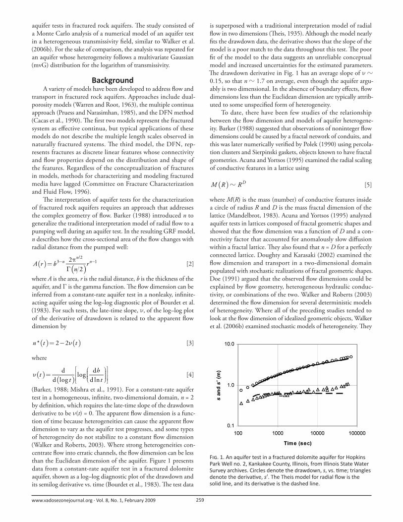
than the Euclidean dimension of the aquifer. Figure 1 presents

data from a constant-rate aquifer test in a fractured dolomite

aquifer, shown as a log–log diagnostic plot of the drawdown and

its semilog derivative vs. time (Bourdet et al., 1983). Th e test data

is superposed with a traditional interpretation model of radial

fl ow in two dimensions (Th eis, 1935). Although the model nearly

fi ts the drawdown data, the derivative shows that the slope of the

model is a poor match to the data throughout this test. Th e poor

fi t of the model to the data suggests an unreliable conceptual

model and increased uncertainties for the estimated parameters.

Th e drawdown derivative in Fig. 1 has an average slope of ν ?

0.15, so that n ? 1.7 on average, even though the aquifer argu-

ably is two dimensional. In the absence of boundary eff ects, fl ow

dimensions less than the Euclidean dimension are typically attrib-

uted to some unspecifi ed form of heterogeneity.

To date, there have been few studies of the relationship

between the fl ow dimension and models of aquifer heterogene-

ity. Barker (1988) suggested that observations of noninteger fl ow

dimensions could be caused by a fractal network of conduits, and

this was later numerically verifi ed by Polek (1990) using percola-

tion clusters and Sierpinski gaskets, objects known to have fractal

geometries. Acuna and Yortsos (1995) examined the radial scaling

of conductive features in a lattice using

( ) DM R R? [5]

where M(R) is the mass (number) of conductive features inside

a circle of radius R and D is the mass fractal dimension of the

lattice (Mandelbrot, 1983). Acuna and Yortsos (1995) analyzed

aquifer tests in lattices composed of fractal geometric shapes and

showed that the fl ow dimension was a function of D and a con-

nectivity factor that accounted for anomalously slow diff usion

within a fractal lattice. Th ey also found that n = D for a perfectly

connected lattice. Doughty and Karasaki (2002) examined the

fl ow dimension and transport in a two-dimensional domain

populated with stochastic realizations of fractal geometric shapes.

Doe (1991) argued that the observed fl ow dimensions could be

explained by fl ow geometry, heterogeneous hydraulic conduc-

tivity, or combinations of the two. Walker and Roberts (2003)

determined the fl ow dimension for several deterministic models

of heterogeneity. Where all of the preceding studies tended to

look at the fl ow dimension of idealized geometric objects, Walker

et al. (2006b) examined stochastic models of heterogeneity. Th ey

F . 1. An aquifer test in a fractured dolomite aquifer for Hopkins Park Well no. 2, Kankakee County, Illinois, from Illinois State Water Survey archives. Circles denote the drawdown, s, vs. me; triangles denote the deriva ve, s′. The Theis model for radial fl ow is the solid line, and its deriva ve is the dashed line.


found that log transmissivity fi elds distributed as a multivari-

ate Gaussian process of moderate variance and as a fractional

Brownian process do not consistently produce fl ow dimensions

less than the Euclidean dimension of the aquifer. Walker et al.

(2006b) also found that, for a site percolation network slightly

above the percolation threshold, the apparent fl ow dimension

oscillates around 1.6 and then tends to 2.0 when the scale of

the aquifer test exceeds the correlation length of the percolation

cluster, consistent with percolation model theory (Stauff er and

Aharony, 1994). Walker et al. (2006b) speculated that a DFN

model with lengths distributed as a power law might result in

noninteger fl ow dimensions persisting for the duration of an

aquifer test. Although there is some suggestion that the intensity

of fracturing is positively correlated with the fl ow dimension (T.

Doe, personal communication, 2006), a literature search failed to

reveal studies that directly relate the fl ow dimension to the length

distributions of fractures.

Aquifer tests are mathematically equivalent to the radial dif-

fusion of heat or contaminants in heterogeneous media, and as

such have been extensively studied. Havlin and Ben-Avraham

(1987) noted that the mean squared radius of displacement, ⟨R2⟩, of particles released from a source could be used to characterize

radial diff usion:

2 kR t? [6]

In a homogeneous medium, we would expect normal (Fickian)

diff usion with a characteristic exponent of k = 1. For disordered

media, Havlin and Ben-Avraham noted that anomalous (slow)

diff usion has often been reported, with k < 1. If diff usion is mod-

eled as a random walk in disordered media, the fractal dimension

of the walk, Dw, is >2 and diff usion is anomalously slow, with

⟨R2⟩ scaling with time as k = 2/Dw. Sahimi (1995, 1996) and

Saadatfar and Sahimi (2002) examined radial diff usion in various

types of fractal media including permeabilities with long-range

correlations, and identifi ed additional diff usive behaviors: super-

diff usive with k > 1 and oscillating with k = f(t). Saadatfar and

Sahimi (2002) did not, however, relate these diff usion behaviors

to aquifer tests or the fl ow dimension. Th e connectivity factor of

the model of Acuna and Yortsos (1995) allows for anomalous dif-

fusion in addition to the geometric eff ects of hydraulic diff usion

on a fractal lattice. Acuna and Yortsos (1995) determined the fl ow

dimension, connectivity factor Dw, and the mass fractal dimen-

sion for several fractal geometries by combining two diff erent

numerical approaches. Th e fi rst approach consisted in estimating

the slopes of both the drawdown and the drawdown derivative

from simulated transient single-phase fl ow aquifer tests using the

analytical solution of O’Shaughnessy and Procaccia (1985) for the

anomalous diff usion equation. Th e second approach consisted in

applying a random walk procedure to solve the diff usion problem.

Combining the slopes obtained in the fi rst approach with the scal-

ing exponent of diff usion k obtained from the second approach

using Eq. [6], they determined the corresponding parameters

to characterize fracture geometry and pressure transient diff u-

sion in fractal media as n = 2D/Dw. Th ey also verifi ed the results

by estimating the fractal dimension of the lattice. Le Borgne et

al. (2004) successfully applied the model of Acuna and Yortsos

(1995) to fi eld data, but the relationship of model parameters to

observed fracture characteristics remains largely unexplored.

Fractal models are natural candidates for describing frac-

tured rocks because observed fracture lengths are widely reported

to have broad distributions (such as a power law) and have no

characteristic length scale (Turcotte, 1986; Bour and Davy, 1997;

Bonnet et al., 2001; Sahimi, 1995). Bonnet et al. (2001) noted

that D ? 1.7 is typically reported for two-dimensional networks

of fractures with a power-law exponent of −2. Bour and Davy

(1997) applied concepts from percolation theory to power-law

networks of fractures in a two-dimensional domain and identifi ed

three regimes of connectivity depending on the exponent in the

power–length-law distribution given by Eq. [1]. For a > 3, the

connectivity is ruled by fractures smaller than the system size;

for a < 1 the connectivity of the fracture network is ruled by the

largest fractures in the system; and for 1 < a < 3, the connectivity

is a function of a and the proportion of large vs. small fractures.

Th ey also showed that under a connectivity characterized by 1 <

a < 3 and a constant fracture density, the percolation parameter

is no longer scale independent and that the connectivity strongly

depends on a characteristic length Lc. Th us, at scales smaller

than Lc, the fracture network is globally below the percolation

threshold, while at scales above Lc, the fracture network possesses

trivial scaling properties similar to those observed by Walker et

al. (2006a) for a site percolation network. In addition, Bour and

Davy (1997) found that for an exponent a > 3, the connected

cluster at the percolation threshold had D = 1.9 in agreement

with percolation theory, and that this was independent of a. For

2 < a < 3, Bour and Davy (1999) showed that under certain con-

ditions, D = a −1, in agreement with King (1983) and Turcotte

(1986). Subsequent studies of permeability for each of these

regimes (de Dreuzy et al., 2001) developed relationships for the

scale dependency of the eff ective permeability and the validity

of the eff ective medium approximation but did not examine the

fl ow dimension.

ApproachTh is study used a Monte Carlo analysis of numerical models

of aquifer tests to analyze the fl ow dimension and hydraulic dif-

fusion, using an approach similar to that of Walker et al. (2006b).

Th e steps in the analysis were: (i) create a transmissivity fi eld T(x)

using a DFN model with a power-law distribution of fracture

lengths; (ii) simulate a constant-rate aquifer test using a fi nite-

diff erence model of transient groundwater fl ow; (iii) estimate the

apparent fl ow dimension n*(t), for the centrally located pumping

well; (iv) estimate the mean square radius of displacement of

a diff usive particle ⟨R2⟩ using a geometrical approach and the

apparent diff usion coeffi cient k*(t) at each time step of the aquifer

test; and (v) estimate the mass fractal dimension D of the fracture

network as a function of ⟨R2⟩.Th e Monte Carlo sequence is repeated for many realiza-

tions to infer the behavior of the fl ow dimension, the scaling of

⟨R2⟩ with time, and the mass fractal dimension. Each realiza-

tion is computationally independent, making the analysis well

suited to distributed computing environments. For this project,

the Monte Carlo simulations were performed using computing

resources from the TeraGrid project (www.teragrid.org/, verifi ed

4 Nov. 2008).

Th e aquifer test was simulated with MODFLOW-2000

(Harbaugh et al., 2000), the USGS fi nite-diff erence model for

transient groundwater fl ow. Th e models of aquifer heterogeneity


were created by adapting algorithms from GSLIB (Deutsch and

Journel, 1998).

Model of Aquifer Heterogeneity (Step 1)Th e fractured rock aquifer was represented by a DFN model

of linear features with homogeneous conductivity whose lengths

follow a power law, set within a matrix of low permeability. In

this study, we used the Boolean approach, where a stochastic

point process generates the centroids of linear features or fractures,

which are attached or “marked” to additional random processes

defi ning the type, shape, size, and orientation of the linear fea-

tures. While the centroids of the linear features representing

fractures are randomly located according to a Poisson distribution,

the required statistics for the fracture lengths and fracture orien-

tations can be inferred in principle from sample distributions of

fi eld data. Th en, the discrete features representing the fractures

of high permeability are embedded in a continuous background

matrix of low permeability. Since we used MODFLOW, it was

necessary to discretize the overall domain into cells, which rep-

resent either a fracture or the background matrix. Hydrologic

properties such as transmissivity, storativity, etc., were assigned to

the cells representing either the fractures or matrix. An extended

“virtual” transmissivity fi eld surrounding the model domain was

used to reduce edge eff ects due to long fractures with their cen-

troids located outside of the model domain. Fracture lengths were

distributed according to the power-law model (Eq. [1]) using a

procedure similar to Bour and Davy (1997), with fracture lengths

truncated at the upper limit by the domain extent and at the

lower limit by the spacing of the fi nite-diff erence grid.

Apparent Flow Dimension (Steps 2 and 3)For the estimation of the apparent fl ow dimension (Step 3), a

constant-rate transient aquifer test was simulated (Step 2) in one

realization of the transmissivity fi eld created in Step 1. Th e well

was assigned to the central node of the grid and constant-head

boundary conditions were imposed on the four sides of the model

domain, which was large enough to avoid boundary eff ects. A

simple fi nite-diff erence approximation in time was used to evalu-

ate Eq. [4], and the apparent fl ow dimension was evaluated from

Eq. [3]. Th e aquifer test was repeated for multiple Monte Carlo

realizations of the transmissivity fi eld, and the mean and 95%

confi dence intervals of the apparent fl ow dimensions, n*, were

used to summarize the ensemble of realizations.

Anomalous Diff usion Coeffi cient (Step 4)Researchers have often studied radial diff usion using the anal-

ogous model of a random walk followed by particles released from

a central location. In such random walk models, the diff usion

process is characterized by the time rate of change of the mean

square radius of displacement ⟨R2⟩ of the particles (Saadatfar and

Sahimi, 2002). To help relate the results of random walk analog

models to the results of this research for the fl ow dimension,

this study estimated R2 at each time step by counting the model

cells with a drawdown larger than a prescribed tolerance, stol.

Th e total area occupied by these cells was set equal to the area of

a circle centered at the pumped well, and the squared radius of

that circle was the estimate of R2 for that time step. Th e estimate

of ⟨R2⟩ is the arithmetic mean of R2 averaged across the Monte

Carlo realizations. Cells representing the low-permeability matrix

between the fractures were included in the estimate if their draw-

down was larger than stol because they could still contribute to

the diff usion of the system. Th e prescribed drawdown tolerance

was at least one order of magnitude larger than the convergence

tolerance for the numerical solver in MODFLOW, and was the

same for all models.

Th e drawdown tolerance, stol, was chosen by noting that the

constant-head model boundaries were just beginning to con-

tribute fl ow at the fi nal time step of the simulation; that is, the

infl uence of the aquifer test had just reached the limits of the

model. Th e tolerance, then, is the drawdown that is observed near

the model boundaries when the boundaries just begin to con-

tribute fl ow. Consequently, the mean radius of displacement R is

always less than the radial distance from the pumped well to the

model boundaries. Th is approach was used rather than an analyti-

cal solution for the radius of infl uence (e.g., Oliver, 1990), which

requires eff ective values for transmissivity and storativity that are

not easily defi ned for highly heterogeneous media. Th e apparent

exponent k(t)* was obtained by fi nite-diff erence approximation

in time for the slope of the logarithmic transform of the scaling

law given by Eq. [6].

Fractal Dimension Analysis (Step 5)It is common in many studies to assess the geometry of a

fracture system by computing D, the mass fractal dimension of

the fractures (Bonnet et al., 2001). In our study, we evaluated D

(Eq. [5]) at diff erent length scales of the aquifer test and explored

its relation to the apparent fl ow dimension and the apparent

exponent of diff usion. Th e circles of investigations were centered

at the pumping well location and the radii were chosen equal to

the value of R estimated in Step 4. Th e mass of fractures M(R)

was estimated by counting the model cells representing a fracture

within radius R of the well.

Model ResultsTh e multiscale nature of fracture networks requires large net-

works to be simulated with a fi ne resolution. Th e fi nite diff erence

grid used in this study had a uniform 1-m spacing to ensure

that the stochastic models were accurately represented, while the

model domain was extensive (3001 by 3001 nodes) to permit

simulating aquifer tests without boundary eff ects. Th e simulated

aquifer is consistent with our prior work (Walker et al., 2006b)

and was loosely based on the Culebra dolomite, a fractured dolo-

mite aquifer found at the Waste Isolation Pilot Plant (WIPP) near

Carlsbad, NM (Holt, 1997). A well withdrawing at a constant

rate of 2.28 × 104 m3/s was assigned to the central node of the

grid, and constant-head boundaries were imposed on the four

sides of the model domain. In all simulations, the fl ow balance

error of MODFLOW-2000 was less than ±0.05% of the outfl ow

or infl ow (see Walker et al., 2006a, for additional details).

Th is work aimed to infer the average behavior of fl uid fl ow

and the pressure transient diff usion of a fracture network with

fractal characteristics. Therefore, the arithmetic means and

normal confi dence intervals of the apparent fl ow dimension, the

apparent exponent k*, and the mass fractal dimension were com-

puted among the Monte Carlo realizations. Walker et al. (2006b)

found that 200 Monte Carlo realizations of both site percola-

tion network (SPN) models and mvG models were suffi cient for

stable estimates of the mean and variance of the apparent fl ow


dimensions. Since the apparent fl ow dimensions of the DFN

model show less variability among realizations than do realiza-

tions of the SPN, we expected that 200 realizations would be

suffi cient for stable estimates comparable statistics in this study.

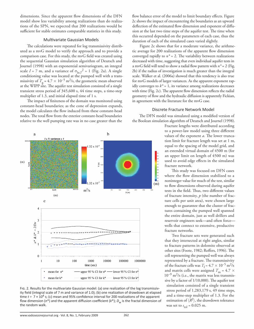
Mul variate Gaussian ModelsTh e calculations were repeated for log transmissivity distrib-

uted as a mvG model to verify the approach and to provide a

comparison case. For this study, the mvG fi eld was created using

the sequential Gaussian simulation algorithm of Deutsch and

Journel (1998) with an exponential semivariogram, an integral

scale I = 7 m, and a variance of σlnT2 = 1 (Fig. 2a). A single

conditioning value was located at the pumped well with a trans-

missivity of Tg = 4.7 × 10−5 m2/s, the geometric mean observed

at the WIPP site. Th e aquifer test simulation consisted of a single

transient stress period of 345,600 s, 44 time steps, a time-step

multiplier of 1.3, and initial elapsed time of 1 s.

Th e impact of fi niteness of the domain was monitored using

constant-head boundaries; as the cone of depression expands,

the model calculates the fl ow induced from these constant-head

nodes. Th e total fl ow from the exterior constant-head boundaries

relative to the well pumping rate was in no case greater than the

fl ow balance error of the model to limit boundary eff ects. Figure

2c shows the impact of encountering the boundaries as an upward

defl ection of the estimated fl ow dimension and exponent of diff u-

sion at the last two time steps of the aquifer test. Th e time when

this occurred depended on the parameters of each case, thus the

duration of each of the simulated cases varied slightly.

Figure 2c shows that for a moderate variance, the arithme-

tic average for 200 realizations of the apparent fl ow dimension

converged rapidly to n* = 2. Th e variability between realizations

decreased with time, suggesting that even individual aquifer tests in

a mvG fi eld will tend to show a radial fl ow pattern with n* = 2 (Fig.

2b) if the radius of investigation is much greater than the integral

scale. Walker et al. (2006a) showed that this tendency is also true

for mvG models of larger variances. As the apparent exponent rap-

idly converges to k* = 1, its variance among realizations decreases

with time (Fig. 2c). Th e apparent fl ow dimension refl ects the radial

geometry of fl ow and the hydraulic diff usion is apparently Fickian,

in agreement with the literature for the mvG case.

Discrete Fracture Network ModelTh e DFN model was simulated using a modifi ed version of

the Boolean simulation algorithm of Deutsch and Journel (1998).

Fracture lengths were distributed according

to a power-law model using three diff erent

values of the exponent a. Th e lower trunca-

tion limit for fracture length was set at 1 m,

equal to the spacing of the model grid, and

an extended virtual domain of 4500 m (for

an upper limit on length of 4500 m) was

used to avoid edge eff ects in the simulated

fracture network.

Th is study was focused on DFN cases

where the fl ow dimension stabilized to a

noninteger value for much of the test, similar

to fl ow dimensions observed during aquifer

tests in the fi eld. Th us, two diff erent values

of fracture intensity, p (the number of frac-

ture cells per unit area), were chosen large

enough to guarantee that the cluster of frac-

tures containing the pumped well spanned

the entire domain, just as well drillers and

reservoir engineers seek—and often force—

wells that connect to extensive, productive

fracture networks.

Two fracture sets were generated such

that they intersected at right angles, similar

to fracture patterns in dolomite observed at

other sites (Foote, 1982; Roff ers, 1996). Th e

cell representing the pumped well was always

represented by a fracture. Th e transmissivity

of the fracture cells was Tf = 4.7 × 10−5 m2/s

and matrix cells were assigned Tm = 4.7 ×

10−9 m2/s (i.e., the matrix was less transmis-

sive by a factor of 1/10,000). Th e aquifer test

simulation consisted of a single transient

stress period of 1,283,179 s, 49 time steps,

and a time-step multiplier of 1.3. For the

estimation of ⟨R2⟩, the drawdown tolerance

was set to stol = 0.025 m.

F . 2. Results for the mul variate Gaussian model: (a) one realiza on of the log transmissiv-ity fi eld (integral scale of 7 m and variance of 1.0); (b) one realiza on of drawdown at elapsed me t = 7 × 104 s; (c) mean and 95% confi dence interval for 200 realiza ons of the apparent fl ow dimension (n*) and the apparent diff usion coeffi cient (k*); Dw is the fractal dimension of the random walk.


Th e infl uence of fracture connectivity on the apparent values

of the fl ow dimension (Eq. [3]), diff usion exponent (Eq. [6]), and

mass fractal dimension (Eq. [5]) was examined using four cases:

two cases in which the exponent a changed while the intensity

p was held constant and two cases where the intensity changed

while the exponent was held constant. Table

1 summarizes the statistics of the fracture

lengths for the four diff erent cases. In gen-

eral, decreasing the exponent a for a constant

intensity parameter increased the frequency

of longer fractures, thus fewer fractures were

necessary to create a connected network that

spanned the domain. Increasing a with a

constant intensity decreased the probability

of having large fractures and the connectiv-

ity was carried by a larger number of smaller

fractures. Consequently, as the exponent a

increased, the mean and median fracture

length in the domain tended to decrease and

the proportion of fracture lengths smaller

than the size of the domain tended to

increase (Table 1). Th is eff ect is clearly seen

in the increased sparseness of the fracture

network as a increased from 1.2 to 2.0 (com-

pare Fig. 3a and 4a). Th e same trend can be

observed in comparing Fig. 5a and 6a, where

a increased from 2.0 to 2.5. Although both

small and large fractures were connected to

the fl owing cluster, the largest fractures con-

trolled the connectivity for a = 1.2 (Case 1)

and the smaller fractures controlled the con-

nectivity when a increased to 2.5 (Case 4), as

noted by Bour and Davy (1997).

Before presenting the detailed results

from the Monte Carlo simulations, it is

instructive to discuss the expected asymp-

totic behavior of the fl ow dimension and

the anomalous diff usion coeffi cient at the

limits of the connectivity regimes when a =

1 and 3. When the exponent a of the power-

law model tends to 1, the connectivity of a

fracture network at an intensity p equal to

that of the percolation threshold is reached

by a few long fractures. For that condition,

we would expect to have a fl ow dimension

n* that tends to 1 (refl ecting the pipe-like

geometry of fl uid fl ow [Barker, 1988]), the

fractal dimension of the network would tend to D = 1, and pres-

sure transients would diff use as a Fickian process. At the other

extreme where exponent a approaches 3, the connectivity of a

fracture network near the percolation threshold arises from a large

number of shorter fractures. For this condition, as the hydraulic

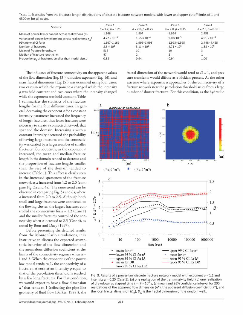
F . 3. Results of a power-law discrete fracture network model with exponent a = 1.2 and intensity p = 0.25 (Case 1): (a) one realiza on of the transmissivity fi eld; (b) one realiza on of drawdown at elapsed me t = 7 × 104 s; (c) mean and 95% confi dence interval for 200 realiza ons of the apparent fl ow dimension (n*), the apparent diff usion coeffi cient (k*), and the local fractal dimension (DR); Dw is the fractal dimension of the random walk.

T 1. Sta s cs from the fracture length distribu ons of discrete fracture network models, with lower and upper cutoff limits of 1 and 4500 m for all cases.

Sta s cCase 1

a = 1.2, p = 0.25Case 2

a = 2.0, p = 0.25Case 3

a = 2.0, p = 0.35Case 4

a = 2.5, p = 0.35

Mean of power-law exponent across realiza ons ⟨a⟩ 1.168 1.997 1.994 2.451

Variance of power-law exponent across realiza ons σa2 4.72 × 10−5 1.55 × 10−4 9.0 × 10−5 4.91 × 10−4

95% normal CI for a 1.167–1.169 1.995–1.998 1.993–1.995 2.448–4.455Number of fractures 8.5 × 103 3.11 × 105 4.71 × 105 1.38 × 106

Mean of fracture lengths, m 512 10 10 3Median of fracture lengths, m 47 2 2 1Propor on ps of fractures smaller than model size L 0.82 0.94 0.94 1.00


test evolves in time, the radius of inspection covers many correla-

tion lengths of the percolation cluster, and the system behaves

as macroscopically homogeneous (for which n* = 2 and k* = 1).

Th erefore, when the exponent a increases, we expect increases in

the fl ow dimension, the exponent of diff usion, and the fractal

dimension (if the fracture system network is near the percola-

tion threshold). Th e percolation threshold can be explained as

the minimum proportion of fracture cells that allow the cluster

to span the entire model domain (Balberg, 1986); moreover, it

was demonstrated that for a constant model size, the percola-

tion threshold should increase as the exponent a increases (Bour

and Davy, 1997). Th erefore, for a constant intensity parameter,

increasing a will reduce the number of connected paths but will

increase the proportion of dead-end fractures; together these tend

to oppose any increase in the fl ow dimension and the exponent

of diff usion.

Table 2 summarizes the eff ect of changing the exponent a for

a constant intensity p and vice versa. Th is table reports the stable

values of fl ow dimension n* and exponent

of diff usion k* averaged across Monte Carlo

realizations within a late time–space range

of the aquifer test. Ranges of the local fractal

dimension DR within the same temporal–

space frame are also included. Stable values

of n* and k* reported in this table were com-

puted using Eq. [3] and [6], respectively, and

averaged across the stable time–space range.

In addition, the reported range of local frac-

tal dimensions DR averaged across Monte

Carlo realizations were computed using Eq.

[5] within the same time–space range. Th e

time–space ranges were obtained by inspec-

tion. In general, the sensitivity to changing

the exponent a also depends on the magni-

tude of the intensity parameter. Th e eff ect of

increasing the exponent a on the fl ow dimen-

sion and the anomalous diff usion coeffi cient

(increasing n* and k*) is counterbalanced by

the eff ect of a constant intensity (see Cases

3 and 4 in particular in Table 2). Increasing

the intensity p while maintaining the expo-

nent a tends to increase the fl ow dimension,

the anomalous diff usive coeffi cient, and the

fractal dimension (see Table 2).

Figure 3c illustrates the results for Case

1 (a = 1.2, p = 0.25). The apparent flow

dimension converged to a noninteger value

<2.0 approximately at time t = 5.2 × 103 s

and remained stable for almost 1.5 log cycles

of the aquifer test. At later times and larger

scales of the aquifer test, the apparent fl ow

dimension tended to steadily increase to 2.0

(Table 2). Th e exponent for the scaling of

diff usion also converged to k* < 1 at later

time and remained approximately stable

even for temporal–spatial scales larger than

in the case of the fl ow dimension (Table 2).

Th e mass fractal dimension steadily increased

with time to a value close to 2. Figures 3b

and 3c show that the drawdown started to show radial geometry

with local dimensions DR between 1.81 and 1.90 for a period

between 1.9 × 104 and 3.5 × 105 s.

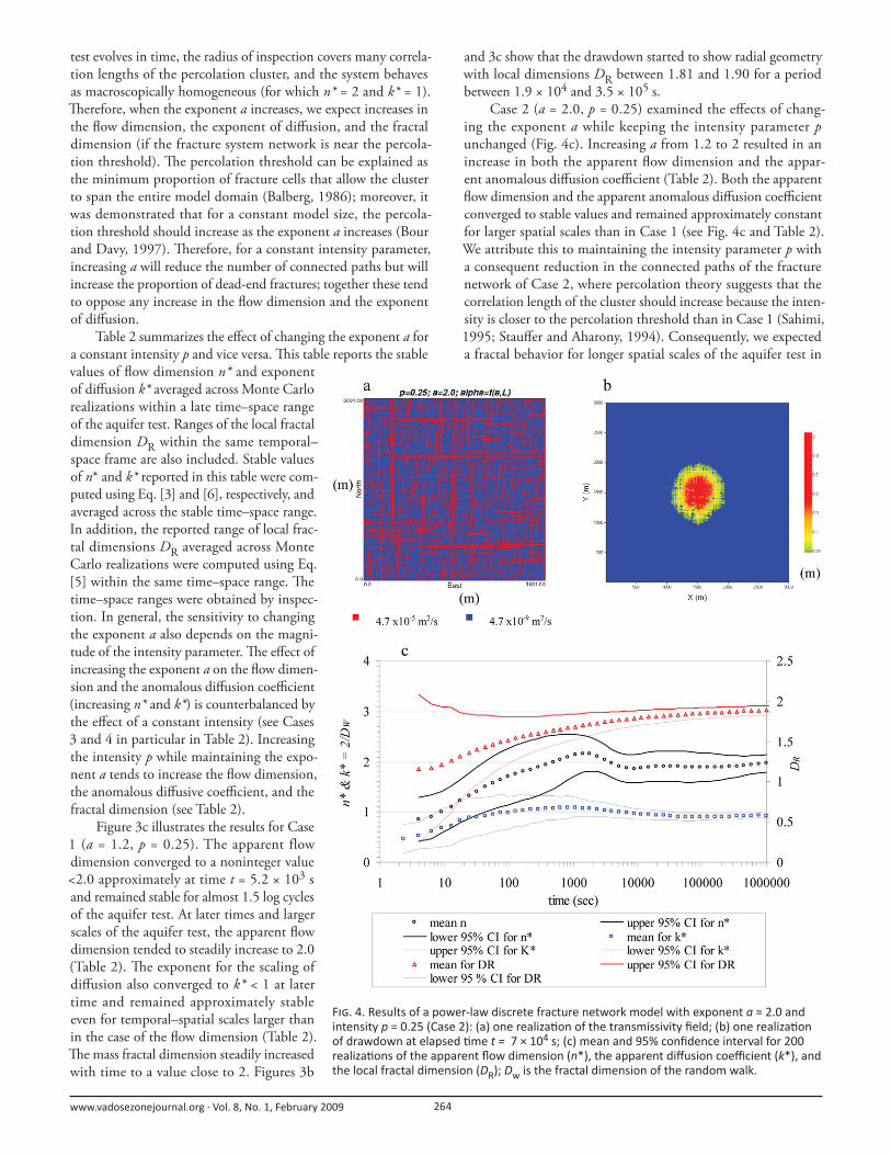
Case 2 (a = 2.0, p = 0.25) examined the eff ects of chang-

ing the exponent a while keeping the intensity parameter p

unchanged (Fig. 4c). Increasing a from 1.2 to 2 resulted in an

increase in both the apparent fl ow dimension and the appar-

ent anomalous diff usion coeffi cient (Table 2). Both the apparent

fl ow dimension and the apparent anomalous diff usion coeffi cient

converged to stable values and remained approximately constant

for larger spatial scales than in Case 1 (see Fig. 4c and Table 2).

We attribute this to maintaining the intensity parameter p with

a consequent reduction in the connected paths of the fracture

network of Case 2, where percolation theory suggests that the

correlation length of the cluster should increase because the inten-

sity is closer to the percolation threshold than in Case 1 (Sahimi,

1995; Stauff er and Aharony, 1994). Consequently, we expected

a fractal behavior for longer spatial scales of the aquifer test in



Case 2 (Table 2). Increasing a tended to increase the mass fractal

dimension, but this eff ect was also counterbalanced by the eff ect

of maintaining the intensity p. Figures 4b and 4c show that the

mass fractal dimension DR was in a range between about 1.82

and 1.88 for a period between 2.5 × 104 and 5.8 × 105 s.

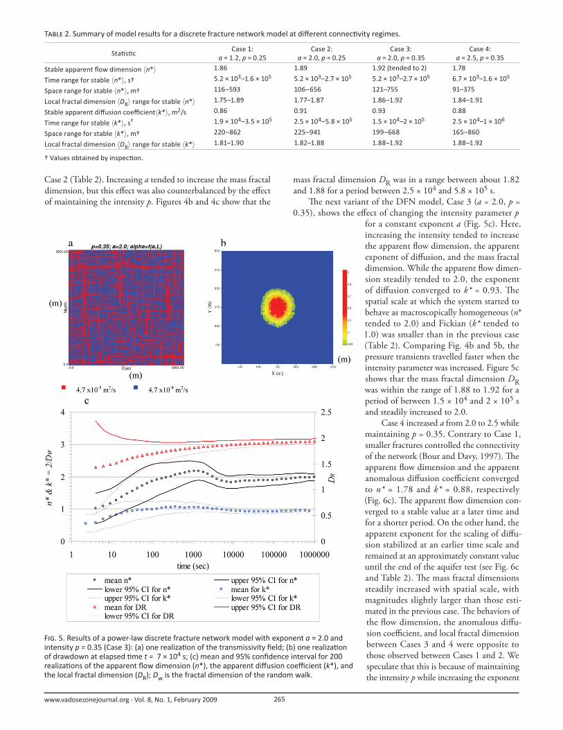
Th e next variant of the DFN model, Case 3 (a = 2.0, p =

0.35), shows the eff ect of changing the intensity parameter p

for a constant exponent a (Fig. 5c). Here,

increasing the intensity tended to increase

the apparent fl ow dimension, the apparent

exponent of diff usion, and the mass fractal

dimension. While the apparent fl ow dimen-

sion steadily tended to 2.0, the exponent

of diff usion converged to k* = 0.93. Th e

spatial scale at which the system started to

behave as macroscopically homogeneous (n*

tended to 2.0) and Fickian (k* tended to

1.0) was smaller than in the previous case

(Table 2). Comparing Fig. 4b and 5b, the

pressure transients travelled faster when the

intensity parameter was increased. Figure 5c

shows that the mass fractal dimension DR

was within the range of 1.88 to 1.92 for a

period of between 1.5 × 104 and 2 × 105 s

and steadily increased to 2.0.

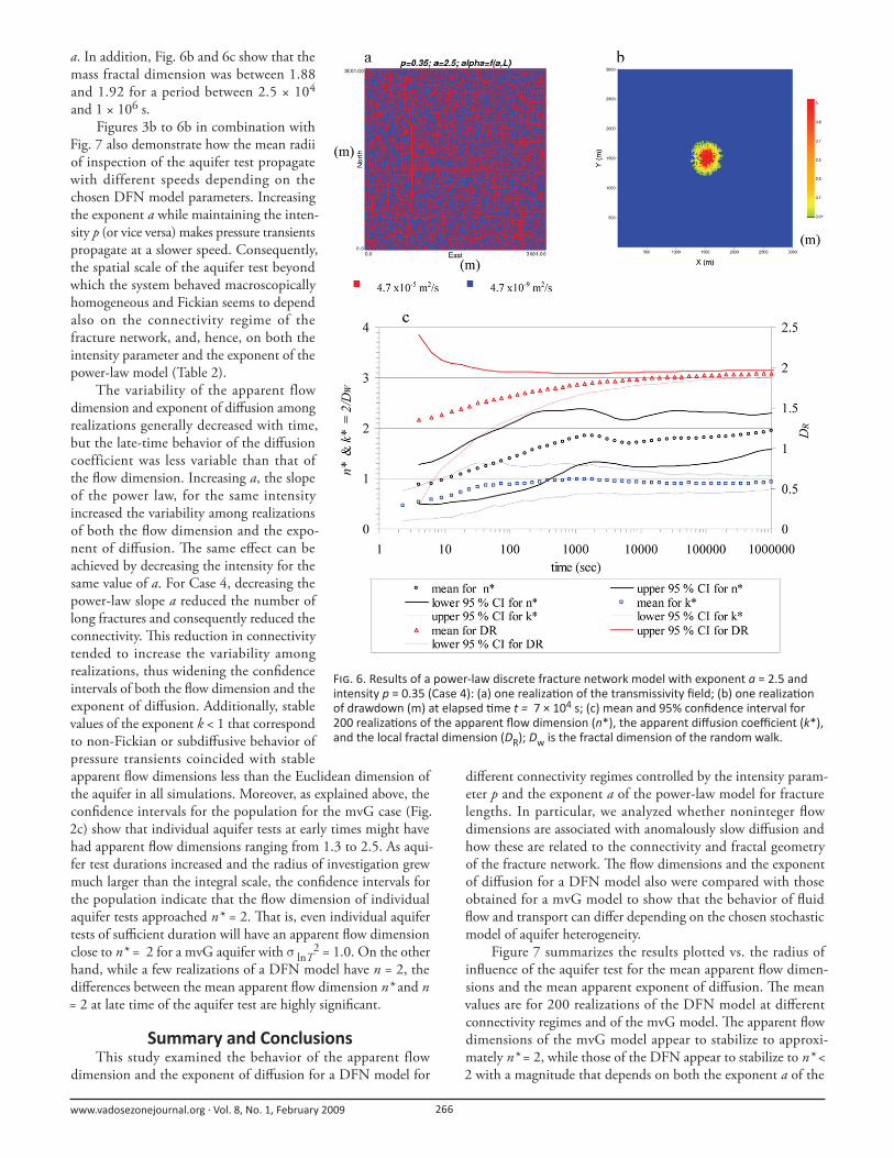
Case 4 increased a from 2.0 to 2.5 while

maintaining p = 0.35. Contrary to Case 1,

smaller fractures controlled the connectivity

of the network (Bour and Davy, 1997). Th e

apparent fl ow dimension and the apparent

anomalous diff usion coeffi cient converged

to n* = 1.78 and k* = 0.88, respectively

(Fig. 6c). Th e apparent fl ow dimension con-

verged to a stable value at a later time and

for a shorter period. On the other hand, the

apparent exponent for the scaling of diff u-

sion stabilized at an earlier time scale and

remained at an approximately constant value

until the end of the aquifer test (see Fig. 6c

and Table 2). Th e mass fractal dimensions

steadily increased with spatial scale, with

magnitudes slightly larger than those esti-

mated in the previous case. Th e behaviors of

the fl ow dimension, the anomalous diff u-

sion coeffi cient, and local fractal dimension

between Cases 3 and 4 were opposite to

those observed between Cases 1 and 2. We

speculate that this is because of maintaining

the intensity p while increasing the exponent


T 2. Summary of model results for a discrete fracture network model at diff erent connec vity regimes.

Sta s cCase 1:

a = 1.2, p = 0.25Case 2:

a = 2.0, p = 0.25Case 3:

a = 2.0, p = 0.35Case 4:

a = 2.5, p = 0.35

Stable apparent fl ow dimension ⟨n*⟩ 1.86 1.89 1.92 (tended to 2) 1.78

Time range for stable ⟨n*⟩, s† 5.2 × 103–1.6 × 105 5.2 × 103–2.7 × 105 5.2 × 103–2.7 × 105 6.7 × 103–1.6 × 105

Space range for stable ⟨n*⟩, m† 116–593 106–656 121–755 91–375

Local fractal dimension ⟨DR⟩ range for stable ⟨n*⟩ 1.75–1.89 1.77–1.87 1.86–1.92 1.84–1.91

Stable apparent diff usion coeffi cient⟨k*⟩, m2/s 0.86 0.91 0.93 0.88

Time range for stable ⟨k*⟩, s† 1.9 × 104–3.5 × 105 2.5 × 104–5.8 × 105 1.5 × 104–2 × 105 2.5 × 104–1 × 106

Space range for stable ⟨k*⟩, m† 220–862 225–941 199–668 165–860

Local fractal dimension ⟨DR⟩ range for stable ⟨k*⟩ 1.81–1.90 1.82–1.88 1.88–1.92 1.88–1.92

† Values obtained by inspec on.


a. In addition, Fig. 6b and 6c show that the

mass fractal dimension was between 1.88

and 1.92 for a period between 2.5 × 104

and 1 × 106 s.

Figures 3b to 6b in combination with

Fig. 7 also demonstrate how the mean radii

of inspection of the aquifer test propagate

with different speeds depending on the

chosen DFN model parameters. Increasing

the exponent a while maintaining the inten-

sity p (or vice versa) makes pressure transients

propagate at a slower speed. Consequently,

the spatial scale of the aquifer test beyond

which the system behaved macroscopically

homogeneous and Fickian seems to depend

also on the connectivity regime of the

fracture network, and, hence, on both the

intensity parameter and the exponent of the

power-law model (Table 2).

The variability of the apparent flow

dimension and exponent of diff usion among

realizations generally decreased with time,

but the late-time behavior of the diff usion

coefficient was less variable than that of

the fl ow dimension. Increasing a, the slope

of the power law, for the same intensity

increased the variability among realizations

of both the fl ow dimension and the expo-

nent of diff usion. Th e same eff ect can be

achieved by decreasing the intensity for the

same value of a. For Case 4, decreasing the

power-law slope a reduced the number of

long fractures and consequently reduced the

connectivity. Th is reduction in connectivity

tended to increase the variability among

realizations, thus widening the confi dence

intervals of both the fl ow dimension and the

exponent of diff usion. Additionally, stable

values of the exponent k < 1 that correspond

to non-Fickian or subdiff usive behavior of

pressure transients coincided with stable

apparent fl ow dimensions less than the Euclidean dimension of

the aquifer in all simulations. Moreover, as explained above, the

confi dence intervals for the population for the mvG case (Fig.

2c) show that individual aquifer tests at early times might have

had apparent fl ow dimensions ranging from 1.3 to 2.5. As aqui-

fer test durations increased and the radius of investigation grew

much larger than the integral scale, the confi dence intervals for

the population indicate that the fl ow dimension of individual

aquifer tests approached n* = 2. Th at is, even individual aquifer

tests of suffi cient duration will have an apparent fl ow dimension

close to n* = 2 for a mvG aquifer with σ lnT2 = 1.0. On the other

hand, while a few realizations of a DFN model have n = 2, the

diff erences between the mean apparent fl ow dimension n* and n

= 2 at late time of the aquifer test are highly signifi cant.

Summary and ConclusionsThis study examined the behavior of the apparent flow

dimension and the exponent of diff usion for a DFN model for

diff erent connectivity regimes controlled by the intensity param-

eter p and the exponent a of the power-law model for fracture

lengths. In particular, we analyzed whether noninteger fl ow

dimensions are associated with anomalously slow diff usion and

how these are related to the connectivity and fractal geometry

of the fracture network. Th e fl ow dimensions and the exponent

of diff usion for a DFN model also were compared with those

obtained for a mvG model to show that the behavior of fl uid

fl ow and transport can diff er depending on the chosen stochastic

model of aquifer heterogeneity.

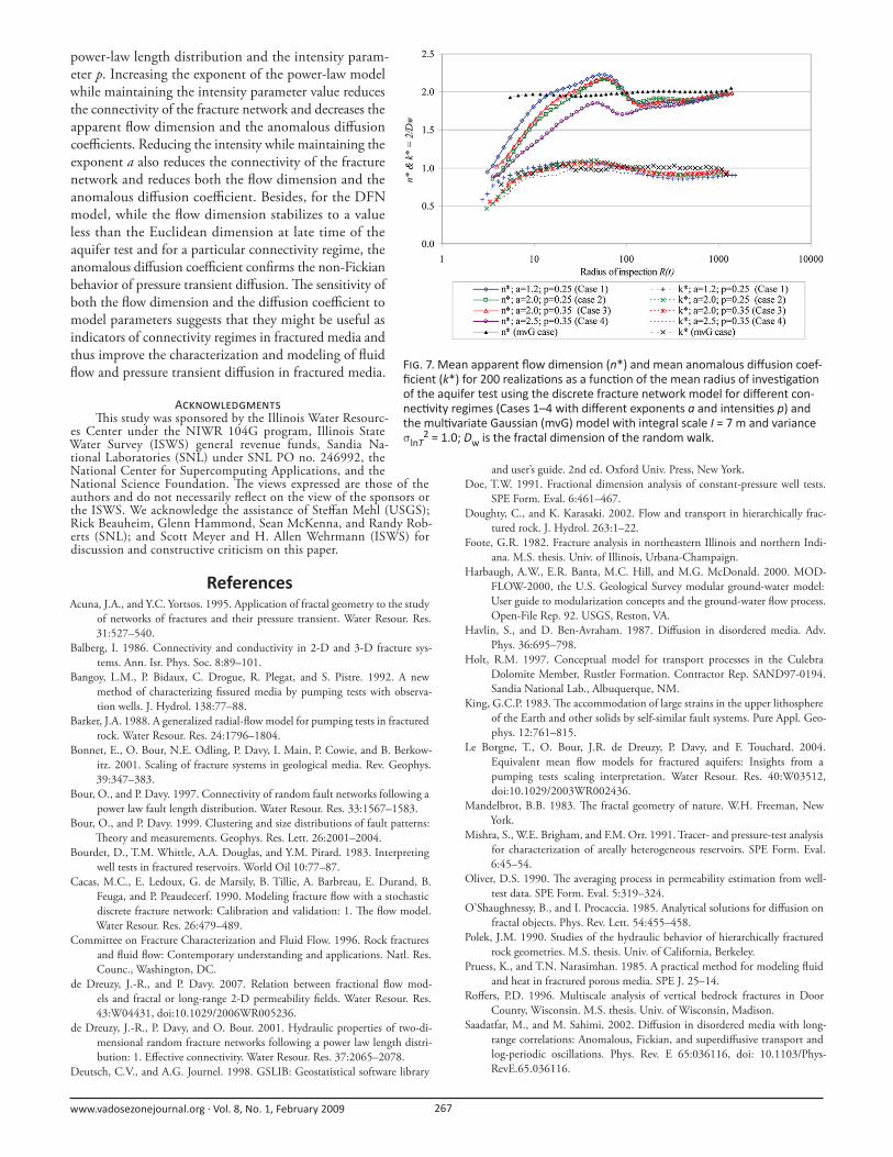
Figure 7 summarizes the results plotted vs. the radius of

infl uence of the aquifer test for the mean apparent fl ow dimen-

sions and the mean apparent exponent of diff usion. Th e mean

values are for 200 realizations of the DFN model at diff erent

connectivity regimes and of the mvG model. Th e apparent fl ow

dimensions of the mvG model appear to stabilize to approxi-

mately n* = 2, while those of the DFN appear to stabilize to n* <

2 with a magnitude that depends on both the exponent a of the

F . 6. Results of a power-law discrete fracture network model with exponent a = 2.5 and intensity p = 0.35 (Case 4): (a) one realiza on of the transmissivity fi eld; (b) one realiza on of drawdown (m) at elapsed me t = 7 × 104 s; (c) mean and 95% confi dence interval for 200 realiza ons of the apparent fl ow dimension (n*), the apparent diff usion coeffi cient (k*), and the local fractal dimension (DR); Dw is the fractal dimension of the random walk.


power-law length distribution and the intensity param-

eter p. Increasing the exponent of the power-law model

while maintaining the intensity parameter value reduces

the connectivity of the fracture network and decreases the

apparent fl ow dimension and the anomalous diff usion

coeffi cients. Reducing the intensity while maintaining the

exponent a also reduces the connectivity of the fracture

network and reduces both the fl ow dimension and the

anomalous diff usion coeffi cient. Besides, for the DFN

model, while the fl ow dimension stabilizes to a value

less than the Euclidean dimension at late time of the

aquifer test and for a particular connectivity regime, the

anomalous diff usion coeffi cient confi rms the non-Fickian

behavior of pressure transient diff usion. Th e sensitivity of

both the fl ow dimension and the diff usion coeffi cient to

model parameters suggests that they might be useful as

indicators of connectivity regimes in fractured media and

thus improve the characterization and modeling of fl uid

fl ow and pressure transient diff usion in fractured media.

ATh is study was sponsored by the Illinois Water Resourc-

es Center under the NIWR 104G program, Illinois State Water Survey (ISWS) general revenue funds, Sandia Na-tional Laboratories (SNL) under SNL PO no. 246992, the National Center for Supercomputing Applications, and the National Science Foundation. Th e views expressed are those of the authors and do not necessarily refl ect on the view of the sponsors or the ISWS. We acknowledge the assistance of Steff an Mehl (USGS); Rick Beauheim, Glenn Hammond, Sean McKenna, and Randy Rob-erts (SNL); and Scott Meyer and H. Allen Wehrmann (ISWS) for discussion and constructive criticism on this paper.

ReferencesAcuna, J.A., and Y.C. Yortsos. 1995. Application of fractal geometry to the study

of networks of fractures and their pressure transient. Water Resour. Res.

31:527–540.

Balberg, I. 1986. Connectivity and conductivity in 2-D and 3-D fracture sys-

tems. Ann. Isr. Phys. Soc. 8:89–101.

Bangoy, L.M., P. Bidaux, C. Drogue, R. Plegat, and S. Pistre. 1992. A new

method of characterizing fi ssured media by pumping tests with observa-

tion wells. J. Hydrol. 138:77–88.

Barker, J.A. 1988. A generalized radial-fl ow model for pumping tests in fractured

rock. Water Resour. Res. 24:1796–1804.

Bonnet, E., O. Bour, N.E. Odling, P. Davy, I. Main, P. Cowie, and B. Berkow-

itz. 2001. Scaling of fracture systems in geological media. Rev. Geophys.

39:347–383.

Bour, O., and P. Davy. 1997. Connectivity of random fault networks following a

power law fault length distribution. Water Resour. Res. 33:1567–1583.

Bour, O., and P. Davy. 1999. Clustering and size distributions of fault patterns:

Th eory and measurements. Geophys. Res. Lett. 26:2001–2004.

Bourdet, D., T.M. Whittle, A.A. Douglas, and Y.M. Pirard. 1983. Interpreting

well tests in fractured reservoirs. World Oil 10:77–87.

Cacas, M.C., E. Ledoux, G. de Marsily, B. Tillie, A. Barbreau, E. Durand, B.

Feuga, and P. Peaudecerf. 1990. Modeling fracture fl ow with a stochastic

discrete fracture network: Calibration and validation: 1. Th e fl ow model.

Water Resour. Res. 26:479–489.

Committee on Fracture Characterization and Fluid Flow. 1996. Rock fractures

and fl uid fl ow: Contemporary understanding and applications. Natl. Res.

Counc., Washington, DC.

de Dreuzy, J.-R., and P. Davy. 2007. Relation between fractional fl ow mod-

els and fractal or long-range 2-D permeability fi elds. Water Resour. Res.

43:W04431, doi:10.1029/2006WR005236.

de Dreuzy, J.-R., P. Davy, and O. Bour. 2001. Hydraulic properties of two-di-

mensional random fracture networks following a power law length distri-

bution: 1. Eff ective connectivity. Water Resour. Res. 37:2065–2078.

Deutsch, C.V., and A.G. Journel. 1998. GSLIB: Geostatistical software library

and user’s guide. 2nd ed. Oxford Univ. Press, New York.

Doe, T.W. 1991. Fractional dimension analysis of constant-pressure well tests.

SPE Form. Eval. 6:461–467.

Doughty, C., and K. Karasaki. 2002. Flow and transport in hierarchically frac-

tured rock. J. Hydrol. 263:1–22.

Foote, G.R. 1982. Fracture analysis in northeastern Illinois and northern Indi-

ana. M.S. thesis. Univ. of Illinois, Urbana-Champaign.

Harbaugh, A.W., E.R. Banta, M.C. Hill, and M.G. McDonald. 2000. MOD-

FLOW-2000, the U.S. Geological Survey modular ground-water model:

User guide to modularization concepts and the ground-water fl ow process.

Open-File Rep. 92. USGS, Reston, VA.

Havlin, S., and D. Ben-Avraham. 1987. Diff usion in disordered media. Adv.

Phys. 36:695–798.

Holt, R.M. 1997. Conceptual model for transport processes in the Culebra

Dolomite Member, Rustler Formation. Contractor Rep. SAND97-0194.

Sandia National Lab., Albuquerque, NM.

King, G.C.P. 1983. Th e accommodation of large strains in the upper lithosphere

of the Earth and other solids by self-similar fault systems. Pure Appl. Geo-

phys. 12:761–815.

Le Borgne, T., O. Bour, J.R. de Dreuzy, P. Davy, and F. Touchard. 2004.

Equivalent mean fl ow models for fractured aquifers: Insights from a

pumping tests scaling interpretation. Water Resour. Res. 40:W03512,

doi:10.1029/2003WR002436.

Mandelbrot, B.B. 1983. Th e fractal geometry of nature. W.H. Freeman, New

York.

Mishra, S., W.E. Brigham, and F.M. Orr. 1991. Tracer- and pressure-test analysis

for characterization of areally heterogeneous reservoirs. SPE Form. Eval.

6:45–54.

Oliver, D.S. 1990. Th e averaging process in permeability estimation from well-

test data. SPE Form. Eval. 5:319–324.

O’Shaughnessy, B., and I. Procaccia. 1985. Analytical solutions for diff usion on

fractal objects. Phys. Rev. Lett. 54:455–458.

Polek, J.M. 1990. Studies of the hydraulic behavior of hierarchically fractured

rock geometries. M.S. thesis. Univ. of California, Berkeley.

Pruess, K., and T.N. Narasimhan. 1985. A practical method for modeling fl uid

and heat in fractured porous media. SPE J. 25–14.

Roff ers, P.D. 1996. Multiscale analysis of vertical bedrock fractures in Door

County, Wisconsin. M.S. thesis. Univ. of Wisconsin, Madison.

Saadatfar, M., and M. Sahimi. 2002. Diff usion in disordered media with long-

range correlations: Anomalous, Fickian, and superdiff usive transport and

log-periodic oscillations. Phys. Rev. E 65:036116, doi: 10.1103/Phys-

RevE.65.036116.

F . 7. Mean apparent fl ow dimension (n*) and mean anomalous diff usion coef-fi cient (k*) for 200 realiza ons as a func on of the mean radius of inves ga on of the aquifer test using the discrete fracture network model for diff erent con-nec vity regimes (Cases 1–4 with diff erent exponents a and intensi es p) and the mul variate Gaussian (mvG) model with integral scale I = 7 m and variance σlnT

2 = 1.0; Dw is the fractal dimension of the random walk.


Sahimi, M. 1995. Flow and transport in porous media and fractured rock: From

classical methods to modern approaches. VCH Verlag, New York.

Sahimi, M. 1996. Linear and nonlinear, scalar and vector transport processes in

heterogeneous media: Fractals, percolation, and scaling laws. Chem. Eng.

J. Biochem. Eng. J. 64:21–44.

Stauff er, D., and A. Aharony. 1994. Introduction to percolation theory. 2nd ed.

Taylor & Francis, Philadelphia, PA.

Th eis, C. 1935. Th e relation between the lowering of the piezometric surface

and the rate and duration of discharge of a well using groundwater storage.

Trans. Am. Geophys. Union 16:519–524.

Turcotte, D.L. 1986. A fractal model for crustal deformation. Tectonophysics

132:261–269.

Walker, D.D., P.A. Cello, A.J. Valocchi, and B. Loftis. 2006a. High-throughput

computing for the analysis of tracer tests in fractured aquifers. Contract

Rep. 2006-4. Illinois State Water Surv., Champaign.

Walker, D.D., P.A. Cello, A.J. Valocchi, and B. Loftis. 2006b. Flow dimensions

corresponding to stochastic models of heterogeneous aquifers. Geophys.

Res. Lett. 33:L07407, doi:10.1029/2006GL025695.

Walker, D.D., and R.M. Roberts. 2003. Flow dimensions corresponding to hy-

drogeologic conditions. Water Resour. Res. 39:1349.

Warren, J.E., and P.J. Root. 1963. Th e behavior of naturally fractured reservoirs.

SPE J. 245–255.

Documents

Flow Dimension and Anomalous Diﬀ usion Ù ã ½Ý of …xanalytica.com/links/papers/VZJ_Cello_2009.pdf · Flow Dimension and Anomalous Di ... its semilog derivative vs. time (Bourdet