Flow Characteristics of Aquatic Ecosystems*

V. CHRISTENSEN and D. PAULYInternational Center for LivingAquatic Resources ManagementMCPO Box 2631, 0718 Makati

Metro Manila, Philippines

CHRISTENSEN, V. and D. PAULY. 1993. Flow characteristics of aquatic ecosystems, p.338-352. In V.Christensen and D. Pauly (eds.) Trophic models of aquatic ecosystems. ICLARM Conf. Proc. 26, 390p.

Abstract

This contribution examines various flow measures based on analysis of 41 quantified models of trophicinteractions in aquatic ecosystems. System productivity/biomass ratio is shown to relate to ecosystem maturityand to the degree of cycling in the systems. Distinct patterns or clusters are observed for different types ofresource systems with respect to average path lengths and residence times. Examination of the averagetrophic transfer efficiencies shows efficiencies of 10-11% for herbivoresldetritivores and first-order predators,and lower efficiencies for higher trophic levels. The overall average transfer efficiency is 9.2%, and thusconfirms the often assumed value of approximately 10% for transfers from one trophic level to the next. Anapproach for estimation of the amount of primary productivity that is required to produce the biomass whichdirectly or indirectly contributes to the fisheries catches is presented and applied to some of the systems.

Introduction

This paper presents some generalizationsbased on a selection of the models in this volumealong with a number of published ECOPATHmodels as adopted for comparisons byChristensen (in press). A number of differentmeasures are examined, notably measuresdiscussed by previous authors, and as such, thispaper somewhat resembles a collage. Our mainintention, however, is to provide some materialfor comparisons for ecosystem modellers wishingto interpret model characteristics, and for thisthe present approach seems appropriate. We donot seek to give comprehensive descriptions ofall attributes, as the present paper is intended tosupplement the contributions of Christensen andPauly (1992a, b), and Christensen (1992, inpress), not to duplicate them.

'ICLARM Contribution No. 832.

Methods and Materials

A total of 41 models were used forcomparisons in this paper (Table 1). The majorityof these are presented in this volume, while afew have been adapted from previously publishedECOPATH models (see Appendix 4). Theselection of models, along with a fewmodifications, follow Christensen (in press). Briefdescriptions of all mode~s can be found in thesame paper. A table giving a summary of the keydata can be found in Christensen (1992) thoughsome of the models were updated between thatpublication and the present.

Very few changes had to be made to themodels to facilitate comparison. The models werestandardized to using g'm-2 wet weight on anannual basis as standard unit, which nearly allalso did beforehand. In addition, bacterial activity

338

339

Table 1. Models used for analysis of flow patterns within ecosystems. The model number and filename are usedfor reference in subsequent tabulations (see also Appendix 4). Where no publication year is indicated under"Source" the reference is to publications included in this volume.

Type and system

Ponds, lakes and rivers1. Mulberry Carp Pond, China2. Laguna de Bay, Philippines, 19683. Laguna de Bay, Philippines, 19804. Lake Kinneret, Israel5. Lake Chad, Africa6. Lake Turkana, Kenya, 19737. Lake Turkana, Kenya, 19878. Lake Victoria, Africa, 1971-19729. Lake Victoria, Africa, 1985-1986

10. Lake Tanganyika, Africa, 1974-197611. Lake Tanganyika, Africa, 1980-198312. Lake Malawi, Africa13. Lake Kariba, Africa14. Lake Ontario, North America15. Lake Aydat, France,16. River Garonne, France17. River Thames, England

Coastal areas18. Etang de Thau, France19. Tamiahua Lagoon, Gulf of Mexico20. Coast, Western Gulf of Mexico21. Campeche Bank, Gulf of Mexico22. Shallow areas, South China Sea23. Lingayen Gulf, Philippines24. Schlei Fjord, Germany25. Mandinga Lagoon, Mexico

Coral reefs26. Bolinao reef flat, Philippines27. French Frigate Shoals, Hawaii28. Virgin Islands, Caribbean

Shelves and seas29. Yucatan shelf, Gulf of Mexico30. Gulf of Mexico continental shelf31. Northeastern Venezuela shelf32. Brunei Darussalam, South China Sea33. Kuala Terengganu, Malaysia34. Gulf of Thailand, 10-50 m35. Shelf of Vietnam/China36. Deep shelf, South China Sea37. Peruvian upwelling system, 1950s38. Peruvian upwelling system, 1960s39. Peruvian upwelling system, 1970s40. Monterey Bay, California41. Oceanic waters, South China Sea

aAs modified by Christensen (in press).

Filename

chinabay68bay80kinneretchadturk73turk87victor71victor85tanga75tanga81ImaIawikaribaontarioaydatgaronnethames

thautamiahuawgmexicocampechethai10lingayenschleimandinga

bolinaoffsvirgin

yucatangomexicovenezuelbruneiterenggathai50vietnamdeepscsperu50peru60peru70montereyoceanscs

Source

Ruddle and ChristensenDe los ReyesDe los ReyesWalline et ai.Palomares et ai.KoldingKoldingMoreau et aI.Moreau et ai.Moreau et ai.Moreau et ai.DegnbolMachena et ai.Halfon and Schitoa

Reyes-Marchant et ai.Palomares et ai.Mathews

Palomares et al.Abarca-Arenas and Valero-PachecoArreguin-Sanchez et ai.Vega-Cendejas et aI.Pauly and Christensen (1993)Pauly and Christensen (1993)Christensen and Pauly (1992b)de la Cruz-Aguero

Alino et al.Polovina (1984)Opitz

Arreguin-Sanchez et ai.BrowderMendozaSilvestre et ai.Christensen (1991)Pauly and Christensen (1993)Pauly and Christensen (1993)Pauly and Christensen (1993)Jarre et ai. (1991)Jarre et ai. (1991)Jarre et ai. (1991)Olivieri et ai.Pauly and Christensen (1993)

was excluded from all models, as they dominatedthe flows of the five systems in which they wereoriginally included.

The number of groups in the different modelsand their distribution by trophic level have notbeen standardized in the present comparisons asthis was not necessary for the kind of analyseshere (Christensen, in press).

Results and Discussion

System Primary Production/Respiration

Odum (1971) described how the ratio betweentotal primary production and total systemrespiration (P/R) would develop as systemsbecome more mature. For immature systems, he

340

assumed that primary production would grosslyexceed total respiration (e.g., for upwellingsystems); he also suggested that the ratio wouldmove toward unity as systems mature. Forsystems where remineralization is a dominantpathway, respiration was expected to exceedprimary production, e.g., for systems receivinglarge amount of organic pollution. H.T. Odumsummarized his description in graphical form,represented here as Fig. 1.

Based on the models given in Table 1, theprimary production/respiration ratio can bequantified. However, we found that the estimateswere not as nicely distributed around the 1:1P :R line, as one might perhaps have expectedCFig. 2). For the majority of the models primaryproductivity exceeds respiration. This, however isnot surprising as primary production is known toexceed respiration in both oceanic systems(Quinones and Platt 1991) and coral reefs (Lewis1981). Table 2 presents a comparison of theliterature estimates reported by Lewis (1981)with the estimates from the present study; asmight be seen, the two data sets display thesame trend, with the bulk of the models havingP /R ratios in the range from 0.8 to 3.2.However, some of the ECOPATH models showhigher values and this warrants a closerexamination.

The seven models with the highest P /R ratio. p(numbers 14, 26, 15, 2, 16, 40, 39) are the onlyones for which the ratio between total export andthe system throughput exceeds 0.3. This points torespiration as the culprit, i.e., to a parameterwhich, in ECOPATH models is estimated as the

difference between consumption and the sum ofproduction and egestion. Quantification ofegestion (or of its converse, assimilation) is oftenquite uncertain; higher egestion leads to lowerrespiration and results in a. higher production ofdetritus. As export from the detritus box inECOPATH models is approximated as thedifference between the flow into the detritus boxand the flow out of the detritus box, an increasedegestion will lead to increased export of detritus.Export of detritus is the only important exportfor practically all models. Therefore it is evidentthat the diverging P /R ratios are due toproblems in model parametrization, specificallyproblems with quantification of assimilation ratesand hence indirectly of respiration.

Adding to the problem of generally high Pp/Rratios is the omission of bacterial activity. Not allthe detritus here assumed to be exported willindeed leave the system. Rather, a large fractionof the detritus will be reutilized by bacteria(which respire!) and thus again made available tothe systems. Therefore omission of bacterialactivity will lead to an underestimation ofrespiration (and of total throughput). One canthus conclude that ECOPATH-type models fromwhich bacterial activity is excluded, can beexpected to overestimate the Pp/R ratios.

System Productivity and Biomass

The ratio of system productivity over biomass(PIB) varies; developing systems tend to have ahigh P/B ratio, due to low biomasses and highproductions, while developed systems tend to

P/R>I Auto.trophy

~ Starting /';., algal culture Coral reefs

0 ,"0 (optimum nutrients) Fertile estuaries

N ,'f; Rich forests

/S' Grasslands ;.,c 10 Fertile /

- .c0 a.+= agriculture Polluted e0 ~ndOrY Ponds streams

....:::J e"0 !low O2 zone)

~0L- '.~ro~"~ Q)a. succession SWQ mp I

1:- watersRich lakes -

0 vE / -""".".~"~ 0::"§. succession "-

I f-' Oceans - 0..<>'

.~ /c:::J

EE Poor lakes0 /u

vsertsRow

sewage

I I0.1

I 10 100

Community respiration (g·m-2 . day-I)

Fig. 1. Position of various communitytypes in a classification based oncommunity metabolism. Gross primaryproduction (P) exceeds communityrespiration (R) on the left side of thediagonal line (P/R > 1 = autotrophy),while the reverse situation holds on theright (PIR < 1 = heterotrophy). The lattercommunities import organic matter orlive on storage or accumulation. Thedirection of autotrophic and heterotrophicsuccession is shown by the arrows. Over ayear's average, communities along thediagonal line tend to consume about whatthey make, and can be considered to bemetabolic climaxes. (Redrawn from Odum1971).

341

The maturity ranking was shown byChristensen (in press) to be stronglycorrelated with total system overheads,which are themselves complementary torelative ascendency. This means thatthere are no contradictions in thefindings of the three studies discussed.

Pimm (1982) examined therelationship between total primaryproduction and system biomass andfound a positive correlation. Theanalysis of the 41 ecosystem modelscompared here shows a pattern similarto that found by Pimm (Fig. 4).

39

40

1~6 2

I I

21

IrJ 104

Respiration (g·rri2. year-I)

14

105

T ...0

~",'

'E 410

!?)

c:0

g16

"85-

10'c:-oEct 41

2 I1010

2

Connectance and SystemFig. 2. Total primary production us total respiration for the 41 models in Omnivory IndexTable 1, to which the numbers refer. The 1:1 line is indicated.

Table 2. Ratio between total primary production andpopulation respiration as reported by Lewis (1981) and in thepresent study.

have high biomasses and lower production rates,giving a lower PIB ratios. This relationship wasdiscussed by Margalef (1968) who, working withmarine phytoplankton, found that perturbationsor fluctuations in the environment cause a shifttoward a state resembling earlier phases ofecosystem development.

These findings are however in contrast tothose of Baird et al. (1991) who could not identifyany relationship between P/B and ascendency(with ascendency assumed to be a measure ofmaturity). Christensen (in press) found that thesystem PIB ratio was useful as one out of eightattributes for derivation of a maturity ranking.Following Christensen's (in press a) approach, ameasure of ecosystem maturity was derived. Toobtain some independence, the maturity rankingin the present analysis was, however, derivedexcluding the system PIB ratio as an attribute.The result is shown in Fig. 3; there is a strongcorrelation between the two measures; usingSpearman's rank correlation gives a highlysignificant coefficient r s = -0.73.

Number of systemswithin the range

p~

Range

<0.80.8-1.61.6-3.23.2-6.4>6.4

In Lewis (1981)

19

123o

In this study

51613

25

Connectance is a measure of theobserved number of food links in a systemrelative to the number of possible links (Gardnerand Ashby 1970). It has been assumed that thereexists an optimum degree of connectance andthat this optimum is dependent on the size of thesystem (Pimm 1982). Other findings suggestedthat the stability of linear systems decreases asthe connectance increases (Martens 1987). Overallthe interpretation of connectance is ambiguous.

The system omnivory index expresses thevariance in the trophic levels of the consumersprey groups (Pauly et al., this vol.) and can beseen as an alternative to the connectance index.The two indices are here found not to besignificantly correlated, and none of them arecorrelated with ecosystem maturity, as shown bythe Spearman rank correlation coefficients, whichare not significant.

Pimm (1982) showed that, as the number ofgroups in a system increases, connectance willdecrease. For the present data set, regressionanalysis gives

C = exp(-0.62 - 0.04 * N),

where C is the connectance and N the number ofgroups in the system. The regression issignificant (0.1%), r 2 = 0.25. This supportsPimm's findings, but also illustrates that only asmall proportion (1/4) of the variability of theconnectance can be explained by the number ofgroups in the system.

Cycling

Cycling is assumed to increase as systemsmature (Odum 1969), and can be quantifiedusing Finn's cycling index (FCI, Finn 1976),

342

200

6

l3cEo:0

"c:.2-g"ea.E.&~

(f)

100

a

2

12 II

14

38

7

40

II

16

35

23

3

31

41

130

4

34

19328 9 33

26 27I

21

36

24

2013 28 25292221 18 17

I ,

31 41

Maturity ranking

Fig. 3. Relationship between system production/biomass ratio and ranking aftermaturity sensu Odum. The ranking used here was derived without using production!biomass as input.

410

28

18 26

36 20

22

21 29

41

3817 18 16 37

25 27 339 2

314 40

624 9 34

85 10 14

716 35 23

32 30 33 1211

19

I I103

10 4

Primary productivity

Fig. 4. System biomass as a function of the total primary production for 41 ecosystemmodels.

which expresses the percentage of the totalthroughput that is actually recycled. The FCIwas not used by Christensen (in press) forquantification of maturity due to its perceivedstrong dependence on model specification, whichmakes intersystem comparisons difficult.

However, ranking the systems after bothmaturity and FCI leads to strong rankcorrelation (rs = 0.56, P < 0.1%). We concludefrom the present analysis that FCI expressessomething that is related to maturity.

Richey et al. (1978) compared four NorthAmerican lakes with different degree of

eutrophication in an effort to evaluate differencesin cycling indices, which were found to varybetween 0.03 and 0.66. While some of the factorsregulating the system structure were apparent,no clear explanations for the varying degree ofcycling could be found, suggesting that cycling initself is not a clear descriptor of ecosystemdevelopment.

Wulff and Ulanowicz (1989) and Baird et al.(1991) were more conclusive: in comparisons ofecosystems these authors concluded that FCI wasmore likely to be an index of stress than ofmaturity. In both studies, however, it was

343

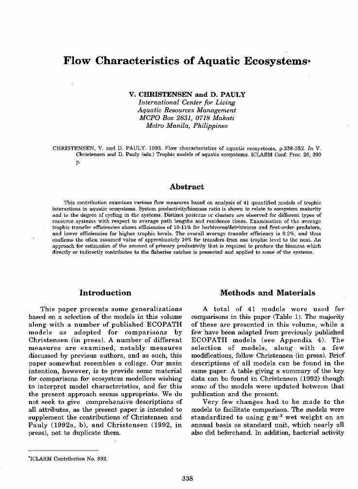
as only six ecosystems are included, notenough to override the variability ofFCI estimates. Cycling is mainly afunction of the degree of detritivory andzero-order cycles ("cannibalism") in asystem, and both are difficult toquantify.

Studying a larger number ofecosystems can be of interest. ThereforeFig. 6 shows a similar plot for the 41ecosystems analyzed in this study .There is some correlation betweencycling index and system overhead (i.e.,ecosystem stability sensu Rutledge et aI.1976). The relationship is perhapsparabolic, and suggests that systemoverheads (stability) decrease at highvalues of the cycling index. Aninterpretation may be that ecosystemswith low cycling (e.g., upwellingsystems) are highly dependent onenergy rapidly passing through and assuch rather unstable and vulnerable tochanges in nutrient input (e.g., throughEI Nino events). On the other hand,systems with a very high cycling maybe less stable because of the need tomaintain an intricate pattern of internalflows. Values intermediate of theseextremes may well be optimal from astability point of view.

Cycling and System Overhead40

• Chesapeake

• Ems

• Ballic

20

Fim's cycling index (%)10

·Peruvian

• Benguela

41

50 26 1614

2

10

40 10

8036 23 4

3234 20

22 17 ,e29

70 9 358 33

21 !9 2420

28 30 640 13

13

6C 3139 10 38

II 2712

37

75

40 o!<--I-~~-----!:lo=------'i'::-5 --:!:~'----::!d5::------:3:!-::lo---:;L35=---40,":-1 ----'45

Finn's cycling index (%)

.Swarlkaps

45

70

~ 6~

"8~ 60

~E 55

ien 50

Fig. 5. System overheads (ecosystem stability) us Finn's cycling index for thesix ecosystems studied by Baird et al. (1991).

It was demonstrated above thatthere is a correlation between cyclingand system overheads (i.e., ecosystem

Fig. 6. System overhead (ecosystem stability) us Finn's cycling index for the stability). It is however not clear if this41 ecosystems in Table 3.

is due to a direct influence of cycling onthe system overheads. To study this we

have included a simulation based on the SchleiFjord ecosystem model (Table 1, No. 24.)

First we removed all cycles from the model,and allocated consumption of detritus tophytoplanktivory. Then w~ gradually increasedthe diet component of detritus for zoobenthosfrom 0 to 60% (the FCI thereby increased from 0to 22%), by increasing the diet component ofdetritus for zooplankton from 0 to 60% (the FCIincreased from 22 to 26%), and finally increasingthe diet component of detritus for both groupsfrom 60 to 99% (the FCI then increased 26 to31%). This led to the results shown in Fig. 7.

It is clear that there is a relationshipbetween the degree of cycling and thesemeasures. System overhead first increases withcycling, levels off, and finally decreases, to some

assumed that relative ascendency was itself ameasure of maturity, following Ulanowicz (1986).

In contrast, the present analysis suggeststhat FCI may be related to maturity sensuOdum. As maturity was shown by Christensen(1992) to be related to stability sensu Rutledge etal. (1976), i.e., to the system overhead (Ulanowicz1986), one can assume that the FCI also shouldrelate to system overhead.

To study this possibility further, we havefirst regressed system stability sensu Rutledge etal. (1976) against FCI for the six systems studiedby Baird et al. (1991).

As can be seen from Fig. 5, this leads toinconclusive results even if the plot indicates thatthere may be a correlation between FCI andstability. The inconclusiveness is not unexpected,

344

length and the straight-through pathlength (Christensen 1992 and seebelow).

Cycling, Primary Productivityand Respiration

135

1

30

14

26

40

39 16

41

31

I I I I

10 15 20 25

Finn's cycling index (%)

Primary productivity

3621

",,--4 ·-·-'

."......... //' System overhead /

//

/Detritus utilization

/o / ,

o 5

100

CD:J 80"0>E:J.§ 60)(

oE'0 40....cCD~

~ 20

100

)(

~ 10

It may be of interest to compareFCI with the primary productivity/respiration (Pf/R) ratio as, based onEppley (1981 , there is an inverserelationship between these indices. Aclose relationship between FCI and PiRdoes exist (see Fig. 8), and that theonly outlier is the model of the oceanicpart of the South China Sea (No. 41), a

Fig. 7. Relationship among system overhead, primary productivity and deep (4,000 m) ecosystem dominated bydetritus utilization, upon the degree of cycling (FeI, all values in %). biomasses flow from the surface towards

the bottom (sedimentation) with verylittle recycling.

Fig. 8 shows that groups with ahigh P IR ratio display a low degree ofrecycling, which is in line with thefindings reported above: P /R movestoward unity and FCI inireases assystems mature. Perhaps the mainconclusion to be drawn here is that thisindicates robustness and mutualconsistency of Odum's (1969) attributesof maturity.

As another system descriptor, wehave estimated the average path length

0.1 O.L,-I.I----~--J:~--------:!~:----------,.:oo for all 41 systems. The path length isPrimary productivity/respiration defined as the average number of

groups that a flow passes through andis calculated as the total throughput

Fig. 8. Finn's cycling index us primary productivity/respiration ratio for the divided by the sum of the exports and41 ecosystem models in Table 1. the respiration (Finn 1980). It appears

that average path length is stronglycorrelated with FCI (Fig. 9). The relationshipbetween cycling rate and path length is notsimply a causal relationship from cycling on pathlength. Christensen (1992) found a strongcorrelation between path length and straight­through path length for the same 41 models. Asthe straight-through path length is calculatedwithout reference to cycling this means that thecorrelation between path length and cycling rateis due to other aspects of the models' structure.

Baird et al. (1991), who compared sixecosystems found that the upwelling systems theystudied had short average path lengths; thesewere longer in the estuarine systems. Fig. 10 wasassembled to allow comparisons of the 41 systemsstudied here.

The majority of the models in Fig. 10 haveaverage path lengths between 2 and 3; 4 have

extent as on Fig. 6. As primary productivity introphic models depends on the food consumptionof the primary consumers, primary productivitywill gradually decline when these consumers shifttowards detritivory.

The findings may at first seem alarmingbecause of the lack of robustness that they seemto imply but it should be recognized thatunrealistic parametrization is very likely to bedetected by careful analysis of the modeldiagnostics. In the present simulation, primaryproductivity provides limits for how much cyclingcan be allowed to vary. It is our conclusion thatthe results mainly serve to increase ourunderstanding of network indices behavior, andthat they do not invalidate the previous findings.This is also supported by the previously reportedresult of a strong correlation between the path

345

Fig. 10. Tropical and temperate ecosystems ranked after path length.

24

24

521

17

,.21 19

401

3629 34

3.530

37 ..

Poth length

Poth length ronklng

27 20

18

6

1917

2~

4

2~3 343629 21

32

33 22

I I I 1 I3 3.5 4 4.5 5

Poth length

I 1012 e 3 9

2.5

133~

115 1614

20

Reefs 26

Tropicalshelves

Tropicalestuaries

OceanlclupwelUng

Tropicalfreshwater

;,0

27 3814 40 IIOI2~7

lal6 39 I ,28o 1262 II I

2 2.5

Temperatefreshwater

Temperateestuaries

40

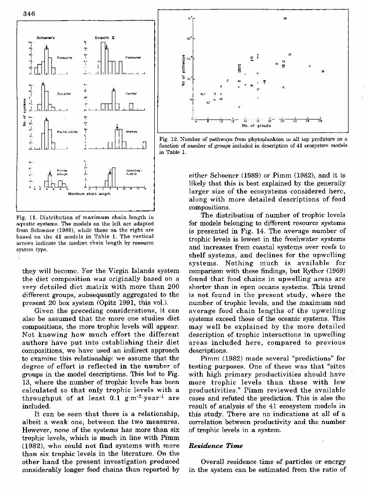
moves from primary producers ordetritus to a top predator. Schoenerfound from a review of 75 aquatic foodwebs that only three webs included foodchains longer than six steps.

Schoener's results are summarizedin Fig. 11 (A-D); this figure alsoincludes maximum chain lengths ascalculated from ECOPATH II using the41 models compared here (E-H). It isevident that the maximum chainlengths in the present study exceedthose in Schoener's study.

I The differences between the two55

studies can to some extent be explainedby the inclusion of a number of verysmall systems in Schoener's study, e.g.,small rockpools and springs. In contrast

Fig. 9. Finn's cycling index us average path length for the 41 ecosystem the present study includes largermodels in Table 1. ecosystems. Another reason may be

related to how detailed the includeddiet compositions are in the models thatare discussed. Schoener stated, "I see asprobably the major problem with webdescription the decision to draw a linkor not. Many species have broad rangesof prey types included in their diet butconcentrate on only a few. 1\.t whatpercent occurrence should a prey nolonger be counted as such?"

In the models included here, allpreys that play a quantitative role(based on weight/volume, not onoccurrence) are included. This to someextent reduces the implied degree ofsubjectivity, but also increases themaximum chain lengths. It is, however,likely that one more explanation mustbe added to explain the differences:many of the present models are made

by biologists with interest in fish populationdynamics, and the upper part of the trophicsystems are therefore better described in thepresent models than in the rockp'ools and othermicrosystems in Schoener's ,study.

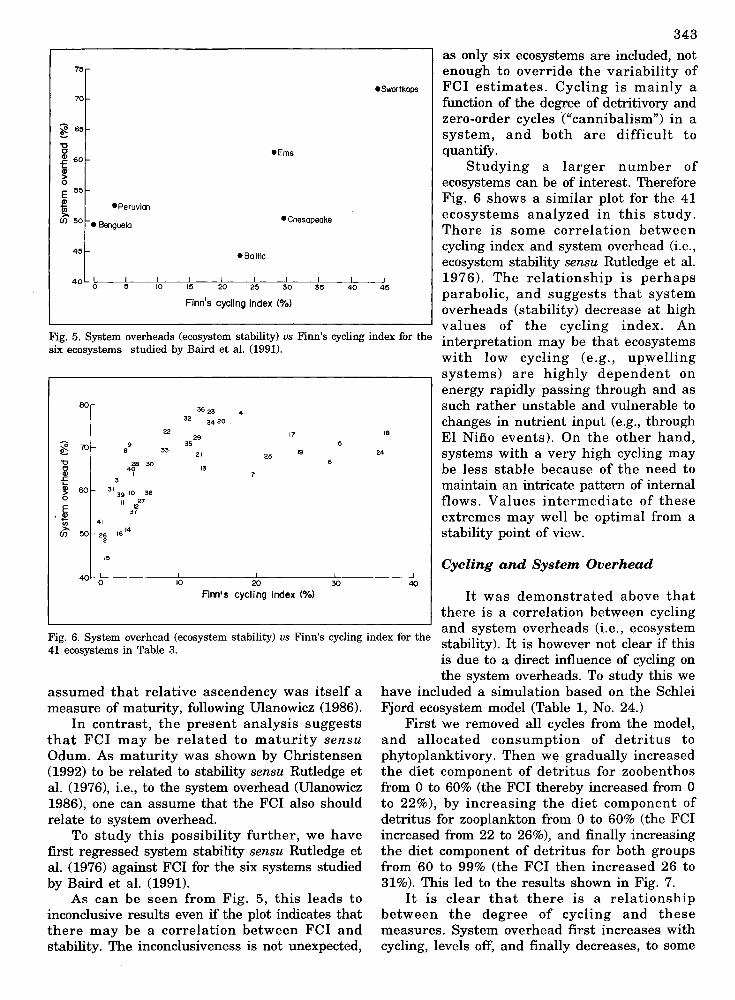
The maximum chain length is not alwayseasy to find when the search for food webs is bytrial-and-error. Fig. 12 shows the total number ofpathways going from phytoplankton to all toppredators for the 41 ecosystem models as afunction of the number of groups in the systems.

One system shows remarkably manypathways, the Virgin Islands coral reefecosystem, which includes 107,618 differentpathways from the phytoplankton. Thisastronomical number illustrates that the moreone studies diet compositions, the more detailed

Schoener (1989) discussed the importance ofmaximum chain length i.e., the number of linksin the longest food chain in a system, when one

Maximum Chain Lengthand Trophic Levels

path lengths between 3 and 4 and only 4 modelshave path lengths that exceed 4. The estuariesand shelves have long path lengths, and the reefsand upwelling/oceanic systems have short pathlengths, which is in agreement with the findingsof Baird et al. (1991). The freshwater systemsspread out over the scale probably because of"lumping" of ecosystems; the marine systemswould do the same had they been pooled in onebig "seawater group".

34610' ,.

26

"

242220

39

22 ~

I I I14 16 18

No. of groups12'0

I I

either Schoener (1989) or Pimm (1982), and it islikely that this is best explained by the generallylarger size of the ecosystems considered here,along with more detailed descriptions of foodcompositions.

10'

~ 103

9

" .'";033£ '"0 ..

Co 3' .~

,0 10' ,.,; '0 , '"z " 30

3

" .'7

10,11 " "10 " "

,6,7

>7

Fig. 12. Number of pathways from phytoplankton to all top predators as afunction of number of groups included in description of 41 ecosystem modelsin Table 1.

Freshwater

Ecoporh II

Maximum chain length

Schoener's

~~.

!Ul~:" 1. ,J~', ,;]~~ ":'-- t, ~'-"., D

:! t Upwelling I2 oceanic

~~. ,.""" "

Fig. 11. Distribution of maximum chain length inaquatic systems. The models on the left are adaptedfrom Schoener (1989), while those on the right arebased on the 41 models in Table 1. The verticalarrows indicate the median chain length by resourcesystem type.

they will become. For the Virgin Islands systemthe diet composition was originally based on avery detailed diet matrix with more than 200different groups, subsequently aggregated to thepresent 20 box system (Opitz 1991, this vol.).

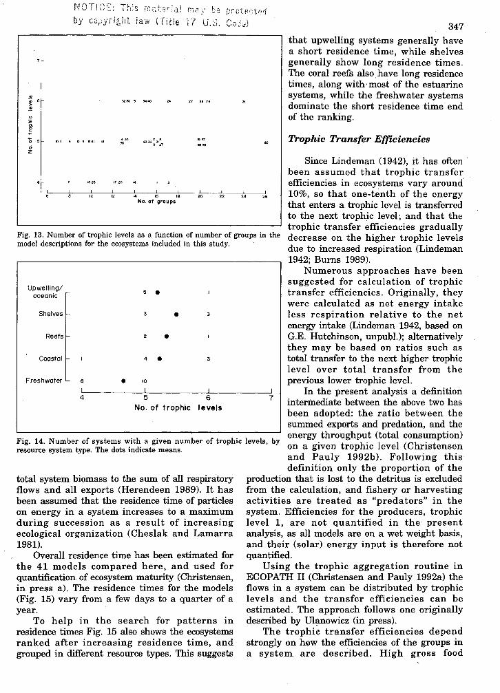
Given the preceding considerations, it canalso be assumed that the more one studies dietcompositions, the more trophic levels will appear.Not knowing how much effort the differentauthors have put into establishing their dietcompositions, we have used an indirect approachto examine this relationship: we assume that thedegree of effort is reflected in the number ofgroups in the model descriptions. This led to Fig.13, where the number of trophic levels has beencalculated so that only trophic levels with athroughput of at least 0.1 g'm-2 'year-1 areincluded.

It can be seen that there is a relationship,albeit a weak one, between the two measures.However, none of the systems has more than sixtrophic levels, which is much in line with Pimm(1982), who could not find systems with morethan six trophic levels in the literature. On theother hand the present investigation producedconsiderably longer food chains than reported by

The dIstnbutlOn of number of trophIc levelsfor models belonging to different resource systemsis presented in Fig. 14. The average number oftrophic levels is lowest in the freshwater systemsand increases from coastal systems over reefs toshelf systems, and declines for the upwellingsystems. Nothing much is available forcomparison with these findings, but Ryther (1969)found that food chains in upwelling areas areshorter than in open oceans systems. This trendis not found in the present study, where thenumber of trophic levels, and the maximum andaverage food chain lengths of the upwellingsystems exceed those of the oceanic systems. Thismay well be explained by the more detaileddescription of trophic interactions in upwellingareas included here, compared to previousdescriptions.

Pimm (1982) made several "predictions" fortesting purposes. One of these was that "siteswith high primary productivities should havemore trophic levels than those with lowproductivities." Pimm reviewed the availablecases and refuted the prediction. This is also theresult of analysis of the 41 ecosystem models inthis study. There are no indications at all of acorrelation between productivity and the numberof trophic levels in a system.

Residence Time

Overall residence time of particles or energyin the system can be estimated from the ratio of

..0; 6>

"":cCl.e'0 5.;Z

NOTI

by

1011 6 1213 1041 18

This rnateria!

law (Title n U. 347

that upwelling systems generally havea short residence time, while shelvesgenerally show long residence times.The coral reefs also. have long residencetimes, along with· most of the estuarinesystems, while the freshwater systemsdominate the short residence time' endof the ranking.

Trophic Transfer Efficiencies

262422

3

3

20

••

3

2

4 •

5 •

10

I I I

14 16 18No. of groups

•

1210

6

Reefs

Coastal

Shelves

Upwellingloceanic

Freshwater

Since Lindeman (1942), it has oftenbeen assumed that trophic transferefficiencies in ecosystems vary around10%, so that one-tenth of the energythat enters a trophic level is transferredto the next trophic level; and that thetrophic transfer efficiencies gradually

Fig. 13. Number of trophic levels as a function of number of groups in the decrease on the higher trophic levelsmodel descriptions for the ecosystems included in this study.

due to increased respiration (Lindeman1942; Burns 1989).

Numerous approaches have beensuggested for calculation of trophictransfer efficiencies. Originally, theywere calculated as net energy intakeless respiration relative to the netenergy intake (Lindeman 1942, based onG.E. Hutchinson, unpubl.); alternativelythey may be based on ratios such astotal transfer to the next higher trophiclevel over total transfer from theprevious lower trophic level.

IL_~ ~I ---L1 ---ll In the present analysis a definition4 5 6 7 intermediate between the above two has

No. of trophic levelsbeen adopted: the ratio between thesummed exports and predation, and theenergy throughput (total consumption)

Fig. 14. Number of systems with a given number of trophic levels, byresource system type. The dots indicate means. on a given trophic level (Christensen

and Pauly 1992b). Following thisdefinition only the proportion of the

production that is lost to the detritus is excludedfrom the calculation, and fishery or harvestingactivities are treated as "predators" in thesystem. Efficiencies for the producers, trophiclevell, are not quantified in the presentanalysis, as all models are on a wet weight basis,and their (solar) energy input is therefore notquantified.

Using the trophic aggregation routine inECOPATH II (Christensen and Pauly 1992a) theflows in a system can be distributed by trophiclevels and the transfer efficiencies can beestimated. The approach follows one originallydescribed by Ul~nowicz (in press).

The trophic transfer efficiencies dependstrongly on how the efficiencies of the groups ina system are described. High gross food

total system biomass to the sum of all respiratoryflows and all exports (Herendeen 1989). It hasbeen assumed that the residence time of particleson energy in a system increases to a maximumduring succession as a result of increasingecological organization (Cheslak and Lamarra1981).

Overall residence time has been estimated forthe 41 models compared here, and used forquantification of ecosystem maturity (Christensen,in press a). The residence times for the models(Fig. 15) vary from a few days to a quarter of ayear.

To help in the search for patterns inresidence times Fig. 15 also shows the ecosystemsranked after increasing residence time, andgrouped in different resource types. This suggests

348

.26

18

17 2e

22

.12

29

26 28 21

..

41

89

.. 112

Overall efficiency 9.2 %

19

18

Residence time (year).03 .06

6 10 .. 3 I

o.

..

3Il 40,37 08

.01

o !--I-----+.------;!2;"-----;3"-----:i4'Rankino after residence time

12

Tropical 6.helwa

Rut. ~

Temperat. 4••tuarles

e~::~f:~ 3

Temperatetr••hwater 2 14

Tropicalt,.lhwaler 1 2 7" 12

...~ 8CIlc

~

~>.glO.91o;;::­Q)

Fig. 15. Residence time for 41 ecosystem models ranked after increasingresidence time. The distribution of each of the models on resource systems isindicated.

conversion efficiencies, GE, corresponding to highp~oduction/consumptionratios, lead to highefficiencies. The gross efficiencies for groups indifferent models are not standardized; one musttherefore expect that the transfer efficiencies asthey appear here will be highly variable. Also,the transfer efficiencies show no correlation at allwith the degree of cycling in the systems.

The analyses were based on the majority ofthe ecosystems described earlier. Systems knownto include fisheries but in which that elementwas not included (most often because of lackingcatch data) were excluded from the analysis. Thenew findings are summarized in Table 3.

From Table 3, a high variability isapparent for the non-African freshwatersystems. For the Chinese pond system,the efficiency on the herbivore/detritivore level is low (5%) as expected,and much higher on the two nextlevels. The low efficiency on level 2 isdue to the inefficient grass carps("manure-machines") feeding on low­quality food in the ponds. Lake Ontarioshows a constant low efficiency of some5%. Lake Aydat has a low efficiency atall levels, apart from on trophic level 4,where there is a peak. The two riversystems show the same pattern, around10% for the herbivores/detritivores, withrapidly declining efficiencies at level 3,and nothing at the higher levels. Forthe two models of Laguna de Bay thepatterns are also similar: from level 2to 3 the efficiencies tend to increase,and then to remain constant. It seemsthat the cultivation of phytoplank­tivorous milkfish (Chanos chanos)resulted as might be expected, inincreased efficiencies on the lowertrophic levels.

The efficiency in Lake Victoriaincreased with the introduction of Nileperch, while the herbivore/detritivoreefficiency in Lake Turkana decreasedradically from 1973 to 1987.

The African lakes to some degree6 21.-1 -----3'-·-----4L-1-----L-~----~6 separate out in low and high efficiency

Trophic level systems, the former represented byLake Tanganyika, Lake Victoria (post­Nile perch) and Lake Chad and the

L-- --l latter by Lake Kariba, Lake Turkana,Fig. 16. Average trophic transfer efficiencies (%) by trophic level based on 37of the models included in the analysis. The vertical bars are ± 1 standard Lake Malawi and Lake Victoria (pre­error. Nile perch). Most of the systems are

characterized by rather high efficienciesat trophic level 2, and graduallydeclining efficiencies at the higherlevels.

Most of the coastal systems, includinglagoons, have rather similar efficiencies of theorder of 10 to 15%. The efficiencies for LingayenGulf are far too high, probably indicatingproblems with model parametrization.

The overall efficiencies for the three coral reefmodels are seen to vary more between thanwithin systems. The transfers are most effectivein the Bolinao model, which is the only one thatincorporates exploitation of the resources. Notingthat the exploitation rate is very high in thissystem, it seems reasonable that the derivedefficiencies should be in the range 9 to 13%. The

349Table 3. Trophic transfer efficiencies (%) for a number of ecosystem models. Only trophic levels with a throughputof at least 0.01 g m-2 year-l and quantified fisheries catches are included.

System

1 2 3 4 5 6 7 8 9Trophic Pond Laguna Laguna Kinneret Chad Turkana Turkana Victoria Victoria

level China 1968 1980 Israel Africa 1973 1987 1971-72 1985-862 5.3 9.8 5.6 19.6 8.8 8.7 4.4 16.0 15.93 12.4 23.1 19.4 8.4 12.6 1.6 5.4 12.3 18.64 13.9 16.7 18.2 3.8 11.5 2.6 0.8 7.0 10.55 16.9 3.2 9.8 0.8 5.4 10.86 8.5

10 11 12 13 14 15 16 17 18 20Tanganyi. Tanganyi. Malawi Kariba Ontario Aydat Garonne Thames Thau Coast

1974-76 1980-83 N.America France France England France Mexico

18.3 13.8 16.9 5.4 4.7 6.6 10.1 8.3 5.3 17.58.6 11.5 2.5 6.5 5.6 2.9 5.3 1.4 13.9 18.6

10.1 11.0 1.6 2.0 4.2 14.1 0.2 0.0 17.3 12.911.2 11.3 0.0 2.2 5.6 16.4 10.0

8.0

21 22 23 24 26 27 28 29 30 31Campeche Coast Lingayen Schlei Bolinao FFS Virgin Yucatan G.o. 'Venezuela

Mexico SCS Phil. Germany Phil. Hawaii Island Mexico Mexico

18.4 6.3 9.4 4.9 9.1 10.1 15.7 15.7 7.6 10.516.8 3.6 10.9 10.3 11.9 4.0 9.5 19.7 15.1 9.113.6 14.6 24.0 8.2 10.3 4.1 6.2 17.6 8.1 4.112.2 15.8 26.8 10.8 3.3 6.1 15.4 4.9 6.011.7 29.6 7.7 8.3

32 33 34 35 36 37 38 39 41Brunei Malaysia G.o. Vietnam Deep Peru Peru Peru Ocean

D. Thailand SCS 1950s 1960s 1970s SCS

15.9 22.7 7.2 3.5 10.8 2.6 2.9 9.3 9.218.7 17.8 15.5 11.7 12.4 9.8 10.6 15.1 12.112.2 14.0 9.7 10.3 9.0 1.8 1.9 7.0 8.06.6 16.2 10.8 7.5 9.0 1.0 0.1 2.4 7.23.5 17.5 13.6

two unexploited reef systems show highestefficiencies for the herbivores/detritivores, andlower on the higher trophic levels.

For the tropical shelf areas some of themodels from Southeast Asia show high transferefficiency. This is partly due to high exploitationrates, but it may also be caused by similarities inmodel construction; this is most apparent for theMalaysian model, whose parameter values wereused in a number of the other models from theregion, including the Lingayen model mentionedearlier to have excessively high efficiencies.

The transfer efficiencies for the upwellingsystems and the oceanic system in Table 3suggest a pattern of low herbivore transferefficiencies, higher efficiencies on trophic level 3and lower efficiencies on the higher levels. It isnoteworthy that the transfer efficiencies of thePeruvian system increased from the 1950s, over

the 1960s, to the 1970s. This increase may bedue to the collapse of the anchoveta (Engraulisringens) and the high exploitation rate (seeJarre-Teichmann 1992 for further discussion).

The two offshore South China Sea modelsshow the same patterns, but as expected theefficiencies are higher in the model covering themore shallow part (Deep SCS). The matchbetween the trends is not likely to be causedprimarily by similarities in the modeldescriptions, but more likely reflects the actualsituation.

Based on the system and trophic level specifictransfer efficiencies the average transferefficiencies fpr the different systems can beestimated (as geometric mean, weighted afterflow). As expected the Mrican lakes fall in twogroups: high and low efficiency systems, withaverage efficiencies of 10-15% and of 2-8%

350

respectively. The distribution of systems on thesegroups is as discussed above.

The three temperate systems, rivers andfjords have rather low average efficiencies, from3 to 7%, while the single temperate lagoon hasan average efficiency within the range of thetropical lagoons and coastal systems, i.e., between10 and 14%. Two coastal areas/shelves, LingayenGulf, and Kuala Terengganu, Malaysia, bothhave very (unrealistic) high efficiencies, 17-18%,probably because of similarities in the modeldescriptions. These systems are not used in thelater generalizations.

The coral reef systems have averageefficiencies in the range of 5-10%, while themodels for the deeper tropical shelf areasgenerally have average efficiencies of 5 to 10%,only the deeper part of the Gulf of Thailand hasa higher efficiency (12%).

The deeper part of the South China Sea andespecially the Peruvian upwelling models are alsoto be found below the 10% efficiency line.

It is difficult to present conclusions regardingoverall trends for ecosystems based on the veryvariable observed efficiencies. One overall systemlevel property can however be estimated: theoverall average transfer efficiencies by trophiclevel based on the 36 models that are discussedhere. Fig. 16 shows an average efficiency of 10%for the herbivores/detritivores, 11% for the nexttrophic level and lower efficiencies (7.5-9.0%) onthe higher trophic levels. The grand meantransfer efficiency for all trophic levels in allsystems is 9.2%, so Lindeman was not far off.

It can be concluded that the trophic transferefficiencies are variable, because of both system­and model-specific characteristics. Generally, thetrophic efficiencies at lower levels (2, 3) tend tobe higher than at higher levels (4-6). In addition,the grand mean trophic transfer efficiency isfound to be very close to the often assumed, butrarely estimated, general rule of 10% per step upthe trophic ladder.

Primary Production Requiredfor the Fisheries

For terrestrial systems, it has been shown byVitousek et al. (1986) that nearly 40% of thepotential terrestrial net primary productivity isused directly or indirectly by human activities.Similar estimates for aquatic systems are notavailable though a rough estimate was presentedin the same publication. The figure given was2%, i.e., much lower than the estimate for theterrestrial systems. It was based on the

assumptions that the "average fish" feeds twotrophic levels above the primary producers; andthat the average food conversion efficiency is 10%at each trophic level.

The crudeness of the approach for the aquaticsystems is due to lack of information especiallyon the trophic positions of the various organismsharvested by humans. Models of trophicinteractions may, however, help to alleviate thesituation, and we suggest here an alternativeapproach based on network analysis, forquantification of the primary productivity neededto sustain harvest by humans.

This approach is based on· quantifieddescriptions of trophic flows in ecosystemnetworks. First, all cycles are remove4 from thediet compositions, and all paths in the flownetwork are identified using the methodsuggested by Ulanowicz (in press). For each paththe flows are then raised to primary productionequivalents using the product of the catch, theconsumption/production ratio of each pathelem~nt times the proportion the next element ofthe path contributes to the diet of the given pathelement. For instance for a path,

Primary producer ~ Herbivore~ Carnivore -1:4 Fishery,

the primary production equivalents correspondingto the catch of 1.2 units are: 1.2·[(1211.2)·1]·[(100/12)·1] = 100, as expected for this simple straightfood chain.

This approach (which will be implemented infuture releases of ECOPATH II) was applied tosome of the ecosystems analyzed in this volume,and the results follow.

For the Peruvian upwelling ecosystem, theharvest in the 1950s required 2% of the availableprimary productivity (PP). In the 1960s, thefishery expanded drastically (14 times) while theprimary productivity requirements (PPR)increased to 5%. The relatively small increase inPPR is mainly caused by the increased catchbeing predominantly anchoveta which isphytoplantivorous, and thus requirecomparatively less PP than organisms on highertrophic levels. The model estimate for the modelfor the Peruvian system in the 1970s pointing tothis model being parametrized with anunrealistically low production/biomass estimatefor bonito (0.03 year-I). This indicates that thepresent analysis may be used as a sensitive toolfor model diagnosis.

For the Laguna de Bay models, total PPRincreased slightly from the late 1960s to the early1980s (from 892 to 941 t ww km-2 year-I). TotalPP, however, decreased considerably due to the

milkfish's consumption of phytoplankton resultingin an increase in utilization of PP from 4 to 11%.

In Lake Victoria, the proliferation of Nileperch resulted in a threefold increase in PPR, tosustain the catches, from some 242 t ww km-2

year-1 in the model from the early 1970s to 742 tww km-2 year-1 in the model for the mid-1980s.

For many of the coastal tropical ecosystemsthe PPR is of the order of a few percentage ofthe total PP, e.g., for the Brunei, Bolinao andVietnam models and for the shallow part of theGulf of Thailand ecosystem. Interestingly, thePPR is higher for the offshore part of the SouthChina Sea (up to as high as 32% for the deepSouth China Sea models). The catches in the off­shore regions are mainly of large pelagics high inthe food web, and thus indirectly requiring alarge fraction of primary productivity.

The method we are proposing here for studyof PPR to sustain catches to some extentparallels a methodology and a concept forvaluation of flows in an ecosystem: emergy, shortfor embodied energy, developed by Odum (1988).Using the emergy concept, it is possible to assigna value to all transfers and for instance comparehow export and import of natural resources froma country compare. The basic principle is thatusing flow specific transfer coefficients all flowsare given in a common currency expressing howmuch energy was used to generate the flows. Thecurrency in the applications we know of has beensolar energy equivalents, see e.g., Brown et al.(1988), and Brown and McClanahan (1992).

The present cursory treatment only gives afirst rough introduction to what can be achievedfrom studies of that part of primary productivitythat is used by humans. We anticipate thatfurther studies will be of use for strategicconsiderations related to our global use ofecological resources.

Conclusion

The present analyses have shown that it ispossible, based on quantified ecosystem models, toestimate characteristics of flow patterns inaquatic ecosystems. We hope that thispreliminary study will encourage new studiesaimed at further refining the analyses, andplacing these in a context where the informationcan be utilized in a management context. Mostnotably the question of how ecosystems are bestutilized needs proper attention. For this,estimation of ecosystem flow patterns is of primeconcern.

351

Acknowledgement

Special thanks to the authors of the modelsincluded in the present study, and to the DanishInternational Development Agency (DANIDA), forfunding and support to the ECOPATH project atICLARM.

References

Baird, D., J.M. McGlade and R.E. Ulanowicz. 1991. Thecomparative ecology of six marine ecosystems. Philos.Trans. R Soc. Lond. 333:15-29.

Brown, M.T. and T.R. McClanahan. 1992. EMergy analysisperspectives of Thailand and Mekong River Damproposals. Report to the Cousteau Society. Center forWetlands and Water Resources, Gainesville, Florida. 60 p.

Brown, M.T., S. Tennenbaum and H.T. Odum. 1988. EMergyanalysis and policy perspectives for the Sea of Cortez,Mexico. Report to the Cousteau Society. Center forWetlands and Water Resources, Gainesville, Florida. 58 p.

Burns, T.P. 1989. Lindeman's contradiction and the trophicstructure of ecosystems. Ecology 70(5):1355-1362.

Cheslak, E.F. and V.A. Lamarra. 1981. The residence time ofenergy as a measure of ecological organization, p. 591-600.In W.J. Mitsch, RW. Bosserman and J.M. Klopatek (eds.)Energy and ecological modelling. Developments inenvironmental modelling. Elsevier, Amsterdam.

Christensen, V. 1991. On ECOPATH, Fishbyte, and fisheriesmanagement. Fishbyte 9(2):62-66.

Christensen, V. 1992. Network analysis of trophic interactionsin aquatic ecosystems. Royal Danish School of Pharmacy,Copenhagen. 55 p. + Appendices. Ph.D. thesis.

Christensen, V. Ecosystem maturity - towards quantification.Ecol. Modelling. (In press a).

Christensen, V. Emergy-based ascendency. Ecol. Modelling. (Inpress b).

Christensen, V. and D. Pauly. 1992a. A guide to theECOPATH II software system (version 2.1). ICLARMSoftware 6, 72 p.

Christensen, V. and D. Pauly. 1992b. ECOPATH II - Asoftware for balancing steady-state models and calculatingnetwork characteristics. Ecol. Modelling 61:169-185.

Eppley, R.W. 1981. Autotrophic production of particulatematter, p. 343-361. In A.R. Longhurst (ed.) Analysis ofmarine ecosystems. Academic Press, New York.' 741 p.

Finn, J.T. 1976. Measures of ecosystem structure and functionderived from analysis of flows. J. Theor. BioI. 56:363-380.

Finn, J.T. 1980. Flow analysis of models of the Hubbard Brookecosystem. Ecology 6:562-571.

Gardner, M.R and W.R. Ashby. 1970. Connectance of large,dynamical (cybernetic) systems. Nature 228:784.

Herendeen, R. 1989. Energy intensity, residence time, exergyand ascendency in dynamic ecosystems. Ecol. Modelling48:19-44.

Jarre, A., P. Muck and D. Pauly. 1991. Two approaches formodelling fish stock interactions in the Peruvianupwelling ecosystem. ICES Mar. Sci. Symp. 193:178-184.

Jarre-Teichmann, A. 1992. Steady-state modelling of thePeruvian upwelling ecosystem. University of Bremen,Bremerhaven, Germany. 153 p. Ph.D. thesis.

Lewis, J.B. 1981. Coral reef ecosystems, p. 127-158. In A.RLonghurst (ed.) Analysis of marine ecosystems. AcademicPress, New York. 741 p.

Lindeman, RL. 1942. The trophic-dynamic aspect of ecology.Ecology 23:399-418.

Margalef, R 1968. Perspectives in ecological theory. UniversityPress, Chicago. 111 p.

352Martens, B. 1987. Connectance in linear and Volterra systems.

Ecol. Modelling 35:157-163.Odum, E.P. 1969. The strategy of the ecosystem development.

Science 164:262-270.Odum, E.P. 1971. Fundamentals of ecology. Saunders,

Philadelphia. 574 p.Odum, H.T. 1988. Self-organization, transformity, and

information. Science 242:1132-1139.Opitz, S. 1991. Quantitative models of trophic interactions in

Caribbean coral reefs. Institut fur Meereskunde, Math­Naturwissenschaftliche, Fakultiit der Christian-Albrechts­Universitiit zu Kiel, Germany.

Pauly, D. and V. Christensen. 1993. Stratified models of largemarine ecosystems: a general approach, and anapplication to the South China Sea, p. 148-174. In K.Sherman, L. M. Alexander and B.D. Gold (eds.) Stress,mitigation and sustainability of large marine ecosystems.AAAS Press, Washington, DC. 376 p.

Pimm, S.L. 1982. Food webs. Chapman and Hall, London. 219p.

Polovina, J.J. 1984. Model of a coral reef ecosystem I. TheECOPATH model and its application to French FrigateShoals. Coral Reefs 3(1):1-11.

Quinones, R.A. and T. Platt. 1991. The relationship betweenthe [-ratio and the P:R ratio in the pelagic ecosystem.Limnol. Oceanogr. 36(1):211-213.

Richey, J.E., R.C. Wissman and AH. Devol. 1978. Carbon flowin four lake ecosystems: a structural approach. Science202:1183-1186.

Rutledge, R.W., B.L. Bacore and R.J. Mulholland. 1976.Ecological stability: an information theory viewpoint. J.Theor. BioI. 57:355-371.

Ryther, J.H. 1969. Photosynthesis and fish production in thesea. Science 166:72-76.

Schoener, T.W. 1989. Food webs from the small to the large.Ecology 70(6):1559-1589.

Ulanowicz, R.E. 1986. Growth and development: ecosystemphenomenology. Springer-Verlag, New York. 203 p.

Ulanowicz, R.E. Ecosystem trophic foundations: Lindemanexonerata. In B.C. Patten and S.E. Jcjlrgensen (eds.)Complex ecology. Prentice Hall, Englewood Cliffs, NewJersey. (In press).

Vitousek, P.M., P.R. Ehrlich, A.H. Ehrlich and P.A. Matson.1986. Human appropriation of the products ofphotosynthesis. BioScience 36: 368-373.

Wulff, F. and R.E. manowicz. 1989. A comparative anatomy ofthe Baltic Sea and Chesapeake Bay ecosystems, p. 232­256. In F. Wulff, J.G. Field and K.H. Mann (eds.) Networkanalysis in marine ecology - methods and applications.Coast. Estuar. Stud. Vol. 32. Springer-Verlag, New York.