NASA Technical Memorandum 105798

Flutter Analysis of Supersonic AxialCascades Using a High ResolutionEuler SolverPart 1: Formulation and Validation

Flow

T.S.R. Reddy and Milind A. Bakhle

University of Toledo

Toledo, Ohio

Dennis L. Huff

Lewis Research Center

Cleveland, Ohio

and

Timothy W. Swafford

Mississippi State University

Mississippi State, Mississippi

August 1992

IW A

Date for general release August 1994

(NASA-TM-IO57OS) FLUTTER ANALYSIS

OF SUOERSONIC AXIAL FLGW CASCAOES

USING A HIGH RESOLUTION EULER

SOLVER. PART I: FORMULATION AND

VALIOATIGN (NASA. Lewis Research

Center) 5b p

N95-1024#

Unclas

G3/39 0022690

https://ntrs.nasa.gov/search.jsp?R=19950003832 2018-05-24T03:35:00+00:00Z

Flutter Analysis of Supersonic Axial FlowCascades Using a High Resolution Euler Solver

Part 1: Formulation and Validation

T. S. R. Reddy *, Milind A. Bakhle **

University of Toledo, Toledo, Ohio 43606

Dennis L. Huff t

NASA Lewis Research Center

Cleveland, Ohio 44135

Timothy W. Swafford÷

Mississippi State UniversityMississippi State, MS

ABSTRACT

This report presents, in two parts, a dynamic aeroelastic stability (flutter) analysis ofa cascade of blades in supersonic axial flow. Each blade of the cascade is modeled as

a typical section having pitching and plunging degrees of freedom. Aerodynamicforces are obtained from a time accurate, unsteady, two-dimensional cascade solver

based on the Euler equations. The solver uses a time marching flux-difference

splitting (FDS) scheme. Flutter stability is analyzed in the frequency domain. The

unsteady force coefficients required in the analysis are obtained by harmonically

oscillating (HO) the blades for a given flow condition, oscillation frequency, and

interblade phase angle. The calculated time history of the forces is then Fourierdecomposed to give the required unsteady force coefficients. An influence coefficient

(IC) method and a pulse response (PR) method are also implemented to reduce the

computational time for the calculation of the unsteady force coefficients for any phase

angle and oscillation frequency. Part 1, this report, presents these analysis methods,and their validation by comparison with results obtained from linear theory for aselected flat plate cascade geometry. A typical calculation for a rotor airfoil is also

included to show the applicability of the present solver for airfoil configurations. The

predicted unsteady aerodynamic forces for a selected flat plate cascade geometry, and

flow conditions correlated well with those obtained from linear theory for differentinterblade phase angles and oscillation frequencies. All the three methods of

predicting unsteady force coefficients, namely, HO, IC and PR showed goodcorrelation with each other. It was established that only a single calculation with

four blade passages is required to calculate the aerodynamic forces for any phaseangle for a cascade consisting of any number of blades, for any value of the oscillation

frequency. Flutter results, including mistuning effects, for a cascade of stator airfoils

are presented in Part 2 of the report.

* Senior Research Associate, Department of Mechanical Engineering** Research Associate, Department of Mechanical Engineeringt Research Engineer+ Associate Professor, Department of Aerospace Engineering

NOMENCLATURE

a

EA]A

b

C

Cl

Cm

%cp

{F}F

G

h

i

i

[I ]Ia

Im{ }

J

kb

[g]KhKa

sonic velocity

matrix of frequency domain aerodynamic coefficients

Roe matrix

airfoil semi-chordairfoil chord

lift coefficient

moment coefficient about elastic axis

pressure coefficient = 2 ( p -p_ ) / pooVoo 2

steady pressure coefficient

unsteady pressure difference coefficient

= ( Plower - Puppet) / P_oV_o2 x amplitude

blade aerodynamic load vector

flux vector in _ direction

flux vector in 77 direction

plunging displacement, normal to airfoil chord

imaginary unit,/_- ; also index in _ direction

incidence angle

identity matrixmoment of inertia about elastic axis

imaginary part of{ }

index in 77 direction

reduced frequency, kb = (9 b/M_ ao_

blade stiffness matrix

spring constant for plunging

spring constant for pitching

lhh , la h, lha , la a

frequency domain unsteady aerodynamic coefficients, Eq. (14)m

M

[M]n

N

NB

NkbN_

qQ

Qh

Qar

rc_

Re{ }

S

sic

Sa

mass of typical sectionMach number

blade mass matrix

blade index

number of blades in the cascade

minimum number of blocks/grids required in computations

number of reduced frequencies used in the analysis

number of interblade phase angles used in the analysisvector of dependent variables

transformed vector of dependent variableslift

moment about elastic axis

index for interblade phase angle, Eq. (12a)

radius of gyration about elastic axis in semi-chord units

real part of{ }

cascade spacing or gap

gap-to-chord ratiostatic unbalance

t

T2t/c

x,y

X_

time

total computational time required for two blocks calculationsthickness-to-chord ratio

Cartesian coordinates

distance between elastic axis and center of mass

in semi-chord units, see Fig. 1

blade displacement vector

reduced velocity, V* = M_ am / b(ga

5

0

P

P

rl

O-

T

A_

fO

(Oh

pitching displacement about elastic axis

difference operator

stagger angle

mass ratio

fluid density

transformed coordinate

transformed coordinate

interblade phase angle

computational time, _ = a_ t /2b

time step

oscillation frequency

uncoupled natural frequency for bending (plunging)

uncoupled natural frequency for torsion (pitching)

subscripts and superscripts

L, R

T

o

O0

n

left, right of interface

transpose of matrixamplitude of harmonic motionevaluated at far upstream conditionsevaluated at time level n

(') d2( ) /dt 2

INTRODUCTION

NASA Lewis Research Center has initiated an exploratory program to investigatethe feasibility of a supersonic through flow (SSTF) fan (Refs. 1-3). The SSTF fan is

expected to provide about a 10 percent decrease in specific fuel consumption, andabout a 25 percent reduction in propulsion system weight, which would lead to a 22

percent increase in aircraft range (Ref. 1). Other advantages of the SSTF fan include

fewer fan stages required for a given pressure ratio, less inlet cowl and boundarylayer bleed drag, better inlet pressure recovery, and better matching of bypass ratio

variation to flight speed. For a safe design of the SSTF fan, analysis is required to

check that dynamic aeroelastic instability or flutter will not occurr in the operating

range. This report presents a flutter analysis for the SSTF fan blade. Only a two-

dimensional (2D) unsteady aerodynamic/aeroelastic analysis has been developedand used, because of the complexity involved in modelling a three-dimensional (3D)rotor / stator in supersonic through flow.

In the 2D unsteady aerodynamic/aeroelastic analysis, the rotor/stator is modelled

as a rectilinear two-dimensional cascade of airfoils with supersonic axial flow

(Refs. 4-8); this is also referred to as a cascade with a supersonic leading edge locus.

Earlier researchers have used linearized equations (see for example Ref. 4)applicable for unloaded cascades of flat plate airfoils in inviscid flow. The motion of

the airfoils in each mode of the cascade is assumed to be simple harmonic with a

constant phase angle between the adjacent blades. This assumption leads to an

eigenvalue problem in the frequency domain and the stability of the system isdetermined from the eigenvalues (Ref. 9).

The above analyses neglect the effects of airfoil thickness, camber, and steady state

angle of attack on supersonic cascade flutter. Recently, an approximate analysis,which includes these effects, was presented in Ref. 10. However, the Mach wave

reflection pattern was assumed to be the same as that for a flat plate cascade. This

means that the effect of the airfoil profile on the Mach wave pattern and its effect on

stability is neglected. One way to rigorously include the effects of airfoil shape

(thickness and camber), and steady state angle of attack in cascade flutter analysis isby using Computational Fluid Dynamics (CFD) methods. Recent advances in the

field of CFD with regard to the development of more efficient algorithms and

increases in computer speed and memory have made numerical studies to computethe complex flow field associated with a supersonic axial flow cascades possible.

Steady aerodynamic characteristics of supersonic compressor airfoils using the

Euler/Navier-Stokes equations have been reported in Ref. 11. Recently, results from

two-dimensional CFD solvers for the analysis of oscillating cascades in supersonicaxial flow have been reported in Refs. 12 and 13. The formulation in Ref. 12 is based

on the full-potential equation, and that in Ref. 13 is based on the Euler equations. Thediscretized form of these equations are solved by the Newton-iteration method for the

full potential equation and by an the alternating direction implicit (ADI) method for

the Euler equations. The unsteady motion resulting from blade oscillation is included

by generating a new grid for every time step in Ref. 12, and by using a deforming grid

technique in Ref. 13. These codes have been extended to include aeroelastic analysisboth in the time and frequency domains in Refs. 14 and 15.

The present study seeks to improve on the work in Ref. 13 in two respects: (a)thesolver of Ref. 13 requires explicit input of artificial viscosity factors to control the

numerical stability of the solution, (b) a C-grid has to be used with this version of theADI solver, which inhibits the true representation of a zero-thickness flat plateairfoil geometry. In order to avoid these difficulties, an Euler solver based on fluxdifference splitting (FDS) has been developed in Ref. 16. This solver does not requireexplicit-input of artificial dissipation factors, and uses an H-grid which allows for atrue representation of flat plate airfoils. This solver was modified to investigateaeroelastic stability of cascadesin subsonic flow in Ref. 17.

The objectives of the present study are (1) to extend the capability of the aeroelasticEuler cascade code of Ref. 17 to predict the unsteady aerodynamic forces of a cascadeof airfoils in supersonic axial flow, (2) to implement influence coefficient and pulseresponse methods (Ref. 18) and verify these for supersonic axial flow cascades bycomparison with other methods, and (3) to use the forces obtained by the abovemethods for flutter calculations of selected supersonic axial flow cascades.

This study is restricted to a two-dimensional cascade model. A typical sectionrepresentation of each of the blades of the cascade is assumed. Two-degrees-of-freedom, plunging and pitching, motion is considered for the analysis. A frequencydomain analysis is used to predict flutter. The study is presented in two parts. Inpart I, this report, the formulation of various methods mentioned in the objectivesabove are presented and validated by comparing with linear theory results, Ref. 8.Typical flutter calculations, for a tuned rotor, are also presented for both a cascade offlat plates and actual SSTF rotor fan airfoils in supersonic axial flow. Extensiveflutter calculations for a cascade of stator airfoils, including mistuning effects, arepresented in part II.

FORMULATION

The aeroelastic model and the aerodynamic model are described in this section.

Aeroe/ast/c model

The aeroelastic model for the cascade consists of a typical section with two degrees of

freedom (bending and torsion) for each blade; see Fig. 1. Structural damping is not

considered at present, although it could be easily included. The equations of motionfor each blade of the cascade have the form:

m]( + Saa" + Khh = Qh (la)

Sa/*" + Iaa" + Kaa = Qa (lb)

where h is the plunging (bending) displacement, a is the pitching (torsion)

displacement, rn is the airfoil mass, Ia is the moment of inertia, Sa is the static

unbalance, Kh and Ka are the spring constants for plunging and pitching,

respectively; Qh and Q(x are the aerodynamic loads (lift and moment, respectively)and the dots over the various terms indicate differentiation with respect to time. The

above equations can be written in matrix notation as

where

[M]-= 1 o_ 0Xa r2a 0 r2a a_a

Qh/mb }{F}=lQa/mb2(3)

and o)h = (Kh/m) 1/2 is the uncoupled natural frequency for bending; ma = (Ka Ha )1/2

is the uncoupled natural frequency for torsion; Xa = Sa/mb is the distance between

the elastic axis and center of mass in semi-chord units; ra = (Ia/mb2) 1/2 is the

radius of gyration about the elastic axis in semi-chord units; and b is the airfoil semi-

chord. The aerodynamic loads, Qh and Qa, are obtained using the aerodynamicmodel described below.

Aerodynamic model

The aerodynamic model is based on the unsteady, two-dimensional, Euler equations.

The equations in conservative differential form are transformed from a Cartesian

reference frame (xff) to a time dependent body-fitted curvilinear reference frame

(_,_7). This transformation process and the ensuing numerical method are presented

in detail in Ref. 19. Hence the following discussion merely highlights thedevelopment of the methodology and the reader is encouraged to consult Ref. 19 formore details.

The transformed Euler equations can be written in vector form as

0Q OF 0G-- + -- + - 0 (4)

37

where

Q =Jq

F =J(_tq + _xf + _yg )

G =J(_Ttq + rlxf + 77yg )

(5a)

(5b)

(5c)

and

q = [p, pu, pv, e ]T

f = [pu,pu2+p,puv,u(e+p)] T

g = [pv,puv,pvZ+p,v(e+p)] T

(5d)

(5e)

(5f)

6

_t , _x , _y , rlt , rlx , and _y are the metrics, p is the fluid density, u and v are thevelocities in Cartesian frame, e is the energy, p is the fluid pressure and J is theJacobian of transformation.

The approach taken in the present effort is based on the integration of these equationsover a discrete set of contiguous cells (volumes) in computational space and is

generally referred to as a finite volume method. This discretization results in the

following expression where cell centers are denoted as i,j :

DQ 8 i F 8j G+ -- + - 0 (6a)

AT

With A_ = Arl = 1 (by definition), this becomes

_T--(SiF + 8jG )

where

(6b)

8i() = ()i+1/2 - ()i-l/2 and 5j() = ()j+l/2 - ()j-l/2

A consequence of the finite volume formulation is that components of the dependent

vector Q within a particular cell represent average values over that cell. However, itis evident from the above representation of flux differences that a method is needed to

allow these fluxes to be accurately represented at cell faces. As discussed in Ref. 19,

the method used in the present effort is based on the one-dimensional Riemannsolver of Roe (Ref. 20) at cell interfaces for each coordinate direction. The method

uses as a basis the following approximate equation which represents a quasilinear

form of a locally one-dimensional conservation law:

-- + A (qL, qR) Dq = 0 (7)_t _x

where q is the untransformed dependent variable vector, and A (qL, qR) is a constant

matrix representative of local cell interface conditions which is constructed using_ so-

called "Roe-averaged" variables. The determination of the eigensystem of A and

knowing that the change in dependent variables across an interface is proportional to

the right eigenvectors allows first order flux formulas to be constructed. This

approach to extracting flowfield information from characteristically dictateddirections is commonly referred to as flux difference splitting (FDS) and is applicable

to multidimensional space if the assumption is made that all wave propagation

occurs normal to a particular cell interface. To provide higher order spatial

accuracy, a corrective flux is appended to the first order flux discussed above. In

addition, in order to control dispersive errors commonly encountered with higherorder schemes, so-called limiters are used to limit components of the interface flux

resulting in total variation diminishing (TVD) schemes. All solutions presentedherein were obtained using third order spatial accuracy in conjunction with the

minmod limiter (Ref. 19).

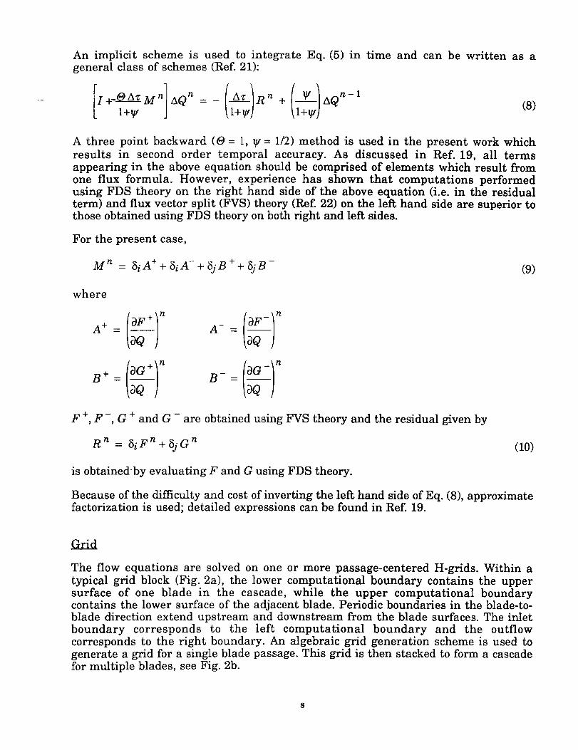
An implicit scheme is used to integrate Eq. (5) in time and can be written as ageneral class of schemes (Ref. 21):

: (8)

A three point backward (8 = l, _, = 1/2) method is used in the present work which

results in second order temporal accuracy. As discussed in Ref. 19, all terms

appearing in the above equation should be comprised of elements which result from

one flux formula. However, experience has shown that computations performed

using FDS theory on the right hand side of the above equation (i.e. in the residual

term) and flux vector split (FVS) theory (Ref. 22) on the left hand side are superior tothose obtained using FDS theory on both right and left sides.

For the present case,

Mn = 5iA+ +SiA-+SJB+ +SJ B- (9)

where

n 0oJ A

F +, F -, G + and G - are obtained using FVS theory and the residual given by

Rn = 5iFn +Sj Gn (10)

is obtainedby evaluating F and G using FDS theory.

Because of the difficulty and cost of inverting the left hand side of Eq. (8), approximatefactorization is used; detailed expressions can be found in Ref. 19.

Grid

The flow equations are solved on one or more passage-centered H-grids. Within a

typical grid block (Fig. 2a), the lower computational boundary contains the upper

surface of one blade in the cascade, while the upper computational boundarycontains the lower surface of the adjacent blade. Periodic boundaries in the blade-to-

blade direction extend upstream and downstream from the blade surfaces. The inlet

boundary corresponds to the left computational boundary and the outflow

corresponds to the right boundary. An algebraic grid generation scheme is used to

generate a grid for a single blade passage. This grid is then stacked to form a cascade

for multiple blades, see Fig. 2b.

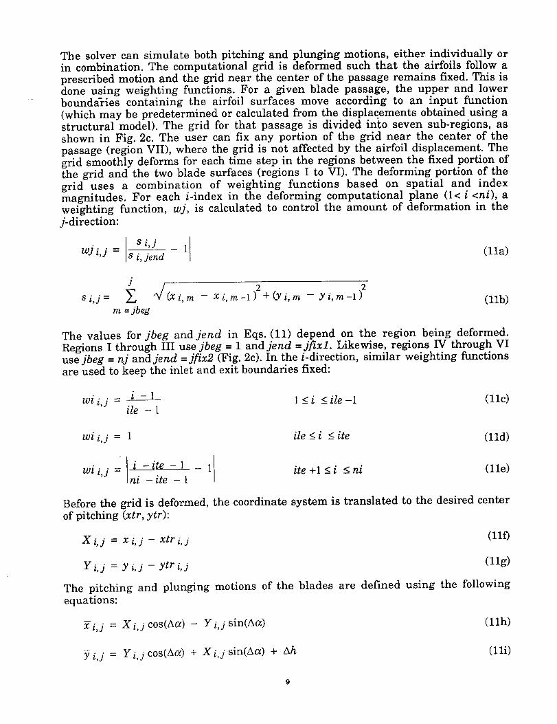
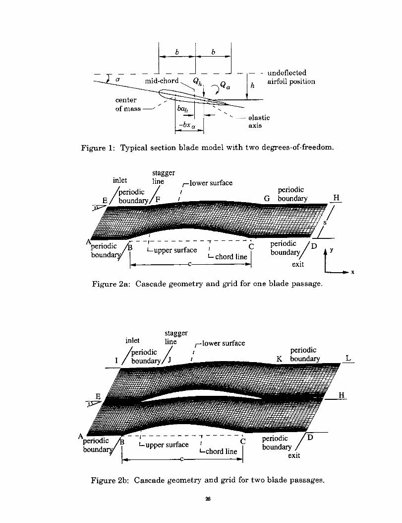
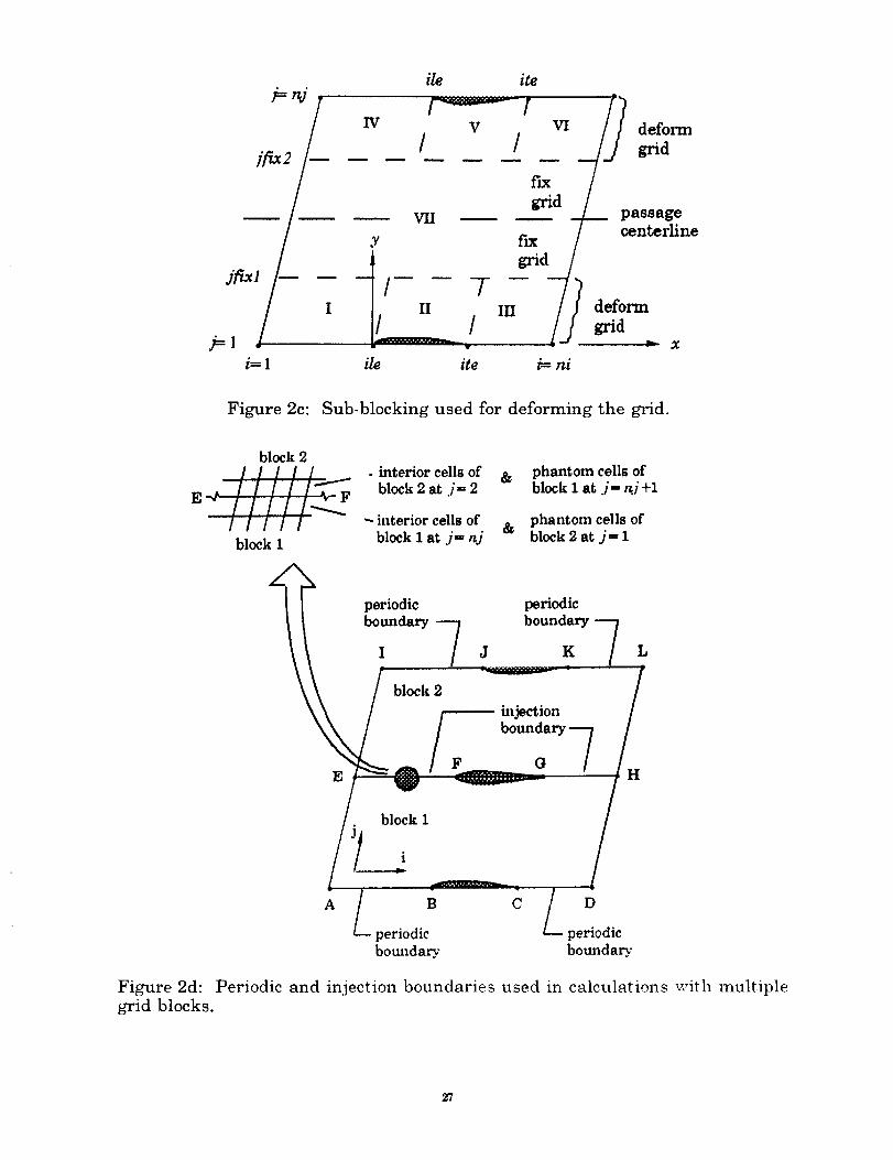
The solver can simulate both pitching and plunging motions, either individually orin combination. The computational grid is deformed such that the airfoils follow aprescribed motion and the grid near the center of the passage remains fixed. This isdone using weighting functions. For a given blade passage, the upper and lowerboundaries containing the airfoil surfaces move according to an input function(which may be predetermined or calculated from the displacements obtained using astructural model). The grid for that passage is divided into seven sub-regions, asshown in Fig. 2c. The user can fix any portion of the grid near the center of thepassage (region VII), where the grid is not affected by the airfoil displacement. Thegrid smoothly deforms for each time step in the regions between the fixed portion ofthe grid and the two blade surfaces (regions I to VI). The deforming portion of thegrid uses a combination of weighting functions based on spatial and indexmagnitudes. For each /-index in the deforming computational plane (l< i <ni), a

weighting function, wj, is calculated to control the amount of deformation in the

j-direction:

s i,j 11 (lla)wj i,j = s i, jend

J

si,j= _., _/(Xi, m - Xi, rn-l_+(Yi, m - Yi, m-1) 2 (11b)

m =jbeg

The values for jbeg andjend in Eqs. (11) depend on the region being deformed.

Regions I through III use jbeg = 1 and jend =jfixl. Likewise, regions IV through VIuse jbeg = nj and jend = jfix2 (Fig. 2c). In the/-direction, similar weighting functions

are used to keep the inlet and exit boundaries fixed:

wi i,j = i - 1 1 <_i < ile -1 (11c)ile - !

wi i,j = 1 ile < i < ite (11d)

l i -ite -1 _ 1wi i,j = ni - ite - iite +1 < i < ni (11e)

Before the

of pitching

grid is deformed, the coordinate system is translated to the desired center

(xtr, ytr):

X i, j = x i, j - xtr i, j(llfl

Y i, j = Y i,j - ytr i,j (11g)

The pitching and plunging motions of the blades are defined using the following

equations:

X i,j = X i,j cos(A60 - Y i,j sin(Aa) (11h)

Y i,j = Y i,j c°s(Aa) + X i,j sin(Aa) + Ah (11i)

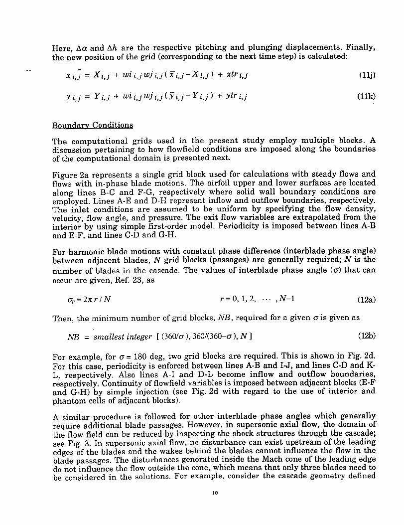
Here, Aa and Ah are the respective pitching and plunging displacements. Finally,

the new position of the grid (corresponding to the next time step) is calculated:

q

x i,j = X i,j + wi i,j wj i, j ( x i,j- X i,j ) + xtr i,j (llj)

Y i,j = Y i,j + wi i,j wj i,j ( Y i,j- Y i,j ) + ytr i, j (11k)

Boundary Conditions

The computational grids used in the present study employ multiple blocks. A

discussion pertaining to how flowfield conditions are imposed along the boundaries

of the computational domain is presented next.

Figure 2a represents a single grid block used for calculations with steady flows and

flows with in-phase blade motions. The airfoil upper and lower surfaces are located

along lines B-C and F-G, respectively where solid wall boundary conditions areemployed. Lines A-E and D-H represent inflow and outflow boundaries, respectively.The inlet conditions are assumed to be uniform by specifying the flow density,

velocity, flow angle, and pressure. The exit flow variables are extrapolated from the

interior by using simple first-order model. Periodicity is imposed between lines A-B

and E-F, and lines C-D and G-H.

For harmonic blade motions with constant phase difference (interblade phase angle)

between adjacent blades, N grid blocks (passages) are generally required; N is the

number of blades in the cascade. The values of interblade phase angle (o-) that can

occur are given, Ref. 23, as

o-r= 2zr / N r=O, 1, 2, ... ,N-1 (12a)

Then, the minimum number of grid blocks, NB, required for a given o- is given as

NB = smallest integer [ (360/o-), 360/(360-o-), N ] (12b)

For example, for o- = 180 deg, two grid blocks are required. This is shown in Fig. 2d.

For this case, periodicity is enforced between lines A-B and I-J, and lines C-D and K-

L, respectively. Also lines A-I and D-L become inflow and outflow boundaries,respectively. Continuity of flowfield variables is imposed between adjacent blocks (E-F

and G-H) by simple injection (see Fig. 2d with regard to the use of interior and

phantom cells of adjacent blocks).

A similar procedure is followed for other interblade phase angles which generally

require additional blade passages. However, in supersonic axial flow, the domain ofthe flow field can be reduced by inspecting the shock structures through the cascade;

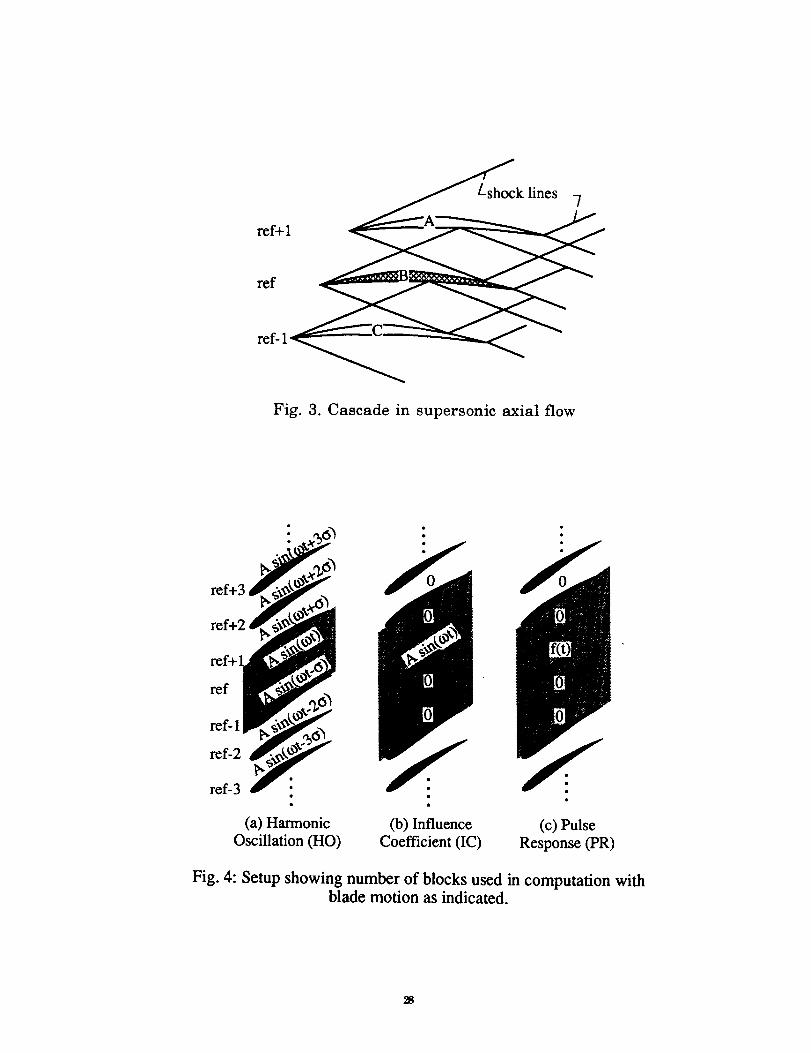
see Fig. 3. In supersonic axial flow, no disturbance can exist upstream of the leading

edges of the blades and the wakes behind the blades cannot influence the flow in theblade passages. The disturbances generated inside the Mach cone of the leading edgedo not influence the flow outside the cone, which means that only three blades need tobe considered in the solutions. For example, consider the cascade geometry defined

10

in Fig. 3, and let the blades be denoted as shown, the blade 'ref' being the reference

blade; let the flow conditions be defined such that the bow shock off the leading edge

intersects the adjacent blade surfaces. The flow above blade 'ref+l' and below blade

'ref-l'will have no influence on the surface pressure on blade 'ref'. For this reason,

the boundary conditions on the upper and lower boundaries, A-B,C-D and I-J, K-L in

Fig. 2d, of the global grid (the grid containing two blocks) can be arbitrary. Thismeans that for harmonic blade motions, only two blocks have to be considered in

computation for any interblade phase angle. However, only the surface pressures onthe reference blade are correct for the specified interblade phase angle.

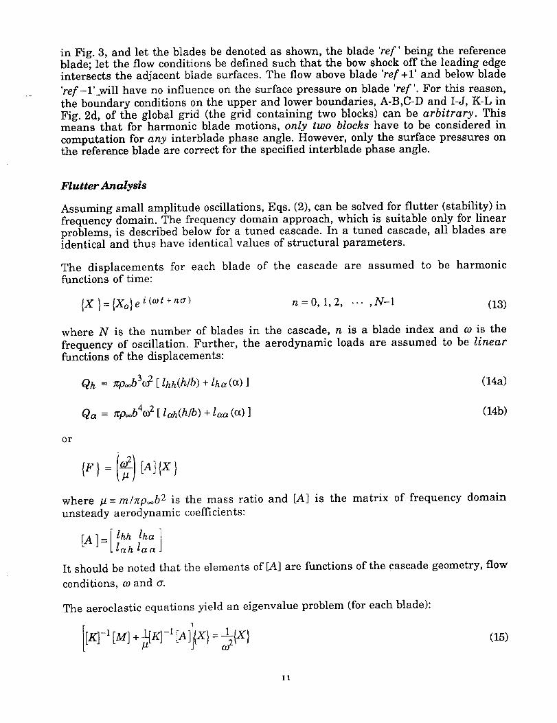
Flutter Analysis

Assuming small amplitude oscillations, Eqs. (2), can be solved for flutter (stability) in

frequency domain. The frequency domain approach, which is suitable only for linearproblems, is described below for a tuned cascade. In a tuned cascade, all blades areidentical and thus have identical values of structural parameters.

The displacements for each blade of the cascade are assumed to be harmonic

functions of time:

{X }= IXo}e i(cot +na) n = 0, 1, 2, ... ,N-1 (13)

where N is the number of blades in the cascade, n is a blade index and co is the

frequency of oscillation. Further, the aerodynamic loads are assumed to be linear

functions of the displacements:

Qh = zP_ 3°]" [ lhh(h/b) + lha (a) ] (14a)

Qa = zpo ob4c°2 [ lah(h/b) + laa (a) ] (14b)

or

where # = m/zp_b 2 is the mass ratio and [A] is the matrix of frequency domain

unsteady aerodynamic coefficients:

lhh lha ][A ]=[ lah laa

It should be noted that the elements of [A] are functions of the cascade geometry, flow

conditions, co and (_.

The aeroelastic equations yield an eigenvalue problem (for each blade):

(15)

11

For a tuned cascade, the same eigenvalue problem is obtained for each blade, Ref. 9.Hence, it is sufficient to solve this problem for just one of the blades (but for each

value of (_). The two eigenvalues obtained from the solution are generally complex.

The real part of the eigenvalue determines the stability of the system; the system issaid to flutter if the real part of either eigenvalue is positive.

The frequency domain aerodynamic coefficients (lhh, lah, etc.) are obtained from the

unsteady Euler solver using one of the three methods described below. These

methods are valid for small amplitude blade oscillations for which the unsteadyflowfield is linearly dependent on the amplitude. A steady flowfield has to be obtained

first for the given cascade geometry (stagger angle, 0 and gap-to-chord ratio, s/c) and

specified inlet conditions (Mach number and incidence angle). Then theaerodynamic coefficients are calculated.

1. Forced Harmonic Oscillation (HO) method

Starting with the steady flowfield, the airfoil motions are specified as sinusoidalvariations in time with a fixed interblade phase angle between adjacent blades:

plunging: h = ho sin( 2kb M_ + nc_ ) (16)

pitching: a = c¢o sin( 2kb M_+ n(_) (17)

n=O, 1,2, ... ,NB-1

where k b = (gb /M_a_ is the reduced frequency based on airfoil semi-chord and

= a_t / 2b is a non-dimensional time.

The Euler equations are marched in time, with the motion as specified above. After

the initial transients have decayed, the lift and moment coefficients show a periodicvariation with time. The variation of the lift and moment coefficients is recorded as a

function of time. This time history is then decomposed into Fourier components to

obtain the complex frequency-domain aerodynamic coefficients. This procedure mustbe done separately for each blade motion - plunging and pitching. It must then be

repeated for each possible value of interblade phase angle. For a cascade with N

blades, the values of interblade phase angle at which flutter can occur are given by'Eq. (12a).

As mentioned earlier, the forced harmonic oscillation method requires only two

blocks for computation for any interblade phase angle. This is true irrespective of thenumber of blades in the cascade. However, the Euler equations have to be solved

separately for each possible interblade phase angle, Eq. (12a). A method to obtain the

coefficients for all possible interblade phase angles in a single calculation isdescribed below.

2. Influence Coefficient (IC) Method

The influence coefficient method, Ref. 18, is based on the principle of linear

superposition and it has been verified experimentally in Ref. 24. Briefly, the solution

12

to a linear problem is obtained by superposing the solutions to the individual

elemental problems that comprise the original problem. Since the method is based on

the principle of linear superposition, it is valid only for linear problems.

The problem to be solved is one of a cascade of N blades in which each blade oscillates

with a motion of the form sin(o) t + n_r ), where n is the blade index that varies from 0

to N -1, and (Yr is the interblade phase angle given by Eq. (12a). This problem is

divided into N elemental problems. The k th elemental problem consists of the same

cascade of N blades in which all blades, except one, are stationary and the k th blade

oscillates with a motion of the form sin(o)t ). The original problem and all the

elemental problems have solutions that are harmonic functions of time.

For the problem in which all blades oscillate with a motion of the form ei( o_t+n_r ), the

forces (Cl and Cm) on the zeroth blade can be represented as Qo eiC°t;Qo is complex

valued to allow the force to lead or lag the motion. Denoting the force on the 0 th blade

in the k th elemental problem as the influence coefficient Qo, k, the force Qo for a given

(Yr is obtained by superposition

Qo ((_r) =

N-1

Qo, k e ik ar

k=O(18)

Further, due to the spatial periodicity of the cascade, only the relative positions of theoscillating blade and the reference (zeroth) blade are important. That is, the forces

generated on the 0 th blade due to the oscillation of the k th blade are equal to the forces

on the 1st blade due to the oscillation of the k+l th blade, and so on. Thus,

Qo, k = Q-k,O = QN-k,O (19)

where the periodicity of the cascade of N blades has been invoked again in the laststep. Eq. (18) can be written in terms of influence coefficients as

N

Q0(o'r) = _ QN-k,O eik_r

k=l(20a)

Replacing the influence coefficients Qo, k by the coefficients QN-k,O means that all

the required influence coefficients can be calculated simultaneously rather than

separately. That is, instead of oscillating the k th blade, calculating the force history

on the 0 th blade and then repeating for all values ofk between 0 and N-I, it is possible

to oscillate the 0 th blade and determine the forces on all blades simultaneously. This

means that the computational effort required for the calculation of all the influence

coefficients can be reduced by a factor of N.

For supersonic axial flow cascades, for which the aerodynamic domain of influence

is contained within the adjacent blade passages, there is no influence on the

reference blade from blades which are more than one blade (pitch) away. Thisindicates that it is sufficient to calculate the correct forces on just three blades,

namely the reference blade and ones on either side. Therefore, Eq. (20) can be writtenas

13

Qref (_r) = Qref, ref + Qref+l,ref e-iar + Qref-l,ref e ia_ (20b)

where the blade indices ref, ref+l and ref-1 refer to the reference blade, the blade

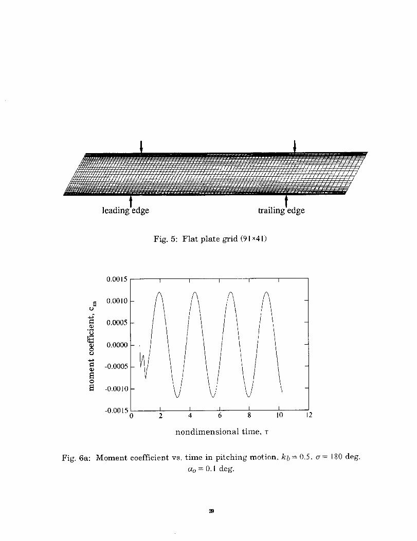
above i't and the blade below it, respectively; see Fig. 4. In the present analysis, four

blocks are used to calculate the unsteady forces on the three blades. Thus, using the

IC method with four blocks in computations, the aerodynamic coefficients can be

calculated for all interblade phase angles at a given oscillation frequency. This is

true irrespective of the number of blades (N) in the cascade. It should be noted that it

is possible to calulate the forces on the three blades using two blocks instead of four;

this requires some code modifications, not attempted here.

The forced harmonic oscillation method and the influence coefficient method require

that the Euler equations have to be solved separately for each oscillation frequency ofinterest. A method to obtain the coefficients for all frequencies in a single calculation

is described below.

3. Pulse Response (PR) method

This method has evolved from the indicial approach that is widely used in many

different fields. The indicial response is the response, lift or moment, to a step

change in the given mode of motion. From the indicial response, the response for anyarbitrary motion, specifically harmonic motion, can be calculated using Duhamers

superposition integral.

Let the time-dependence of the blade motion be denoted as f(t) and let the

corresponding response be denoted as F(t). Let Fs(t) denote the response

corresponding to a unit step function, f (t) = 5(t). The response corresponding to an

arbitrary motion f(t) can be written using Duhamel's superposition integral:

F(t) = f_ F8 (t -_ ) f (_) d_ (21)

Using the above equation, the response to a harmonic motion, f(t)= e ia_t, can be

determined:

_0 tF(t) = Fs(t -_) iwe io_ _d_ (22)

Since only periodic response is desired, consider the above integral in the limit as

t _ oo . Using a change of variable and extending the lower limit to --_, gives

F(t) = io_ F---88(co) e io_ t (23)

where F-8(w) is the Fourier transform of Fs(t) given as

14

r+oo

F---55(o))= J__ Fs(t) e- ico t dt(24)

q

For an arbitrary motion f(t) and the corresponding response F(t), the Fourier

transform of Eq. (21) gives:

g(o_) = ioJ Fs(co) f(o_)

or

i <,., = / (25)

where f(co) and F--(o)) are the Fourier transforms off(t) and F(t), respectively. Eq. (25)

indicates that the response to harmonic blade motion can be determined using any

arbitrary motion f (t) and the corresponding response F(t).

Over the course of time, to avoid numerical difficulties, the step change in

displacement has been replaced by a smooth step function and finally by a pulse. In

the pulse motion, the blade returns to its original position after the duration of the

pulse. This is in contrast to the step motion in which the blade positions are differentbefore and after the step. The pulse motion thus allows the flowfield to return to its

steady undisturbed state after the transients created by the pulse have decayed. The

unsteady calculations therefore need to be carried out only long enough to ensurethat the solution has reached its final state (the same as the initial state) within some

specified tolerance.

Out of the different pulse shapes investigated, Ref. 18 has suggested use of the

following pulse which is used in the present calculations:

' )f(t) = 4 trhax 1 - t 7tmax

f(t) = 0

for0 <t < tmax

for t > tmax

(26)

where tmax is the duration of the pulse. The above choice makes f(t) and f(t) vanish at

t = 0 and t = tmax ; in addition, higher derivatives also go to zero at t = tmax • This

ensures that there is a smooth transition to and from the undisturbed blade position.

The pulse response method can be used in conjunction with the influence coefficientmethod to obtain the frequency domain aerodynamic coefficients for each possible

interblade phase angle and for specified frequencies of oscillation, as follows. Oneblade in the cascade is given a transient motion of the form h(t)= hof(t) or

a (t) = a o f (t). The calculations start with the steady solution and unsteady response

to the pulse in either motion, plunging or pitching, is calculated until the transientflowfield reaches the steady flowfield within a specified tolerance. The motion as well

as the response on all the blades (four in this case) are recorded and Fourier

15

transforms of these are calculated numerically for the frequency of interest. Using

these transforms, the influence coefficients (Qk, o) are calculated from Eq. (25); it is to

be noted that the harmonic response, io)Fa(o_), obtained from Eq. (25) for this case, is

simply-the influence coefficient (Qk,o). Eq. (20b) is then used to calculate the

frequency domain unsteady aerodynamic coefficients for the interblade phase angleof interest. In this way, the coefficients can be determined for various values of

reduced frequency by calculating the Fourier transforms for the frequency of interest

using the same time histories.

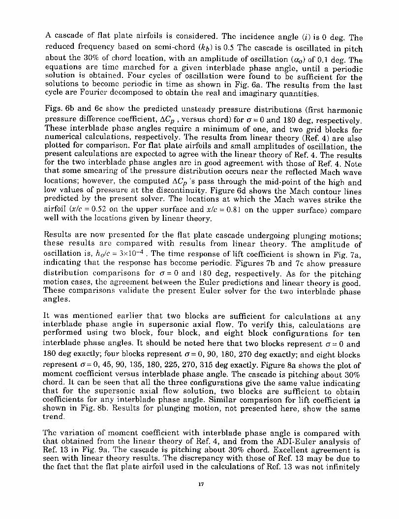
The computational implementation of the three methods, HO, IC and PR, is shown

in Fig. 4. It shows the number of blocks used, and the associated blade motion.

_TS

The analysis methods presented in the previous section are applied to investigate thebehavior of oscillating cascades in supersonic axial flow. First, unsteady pressuredistributions are calculated for a flat plate cascade using the forced harmonic

oscillations (HO) method, Eqs. (16) and (17); the results are compared with published

results to help validate the Euler solver. Then, the unsteady lift and moment

coefficients are compared with those obtained from the influence coefficient (IC)

method and the pulse response (PR) method. Next, frequency domain flutter

calculations are performed for a flat plate cascade and the results are verified by

comparison with results from linear theory. Finally, flutter predictions are

presented for a rotor airfoil cascade, oscillating in coupled pitching and plungingmotion.

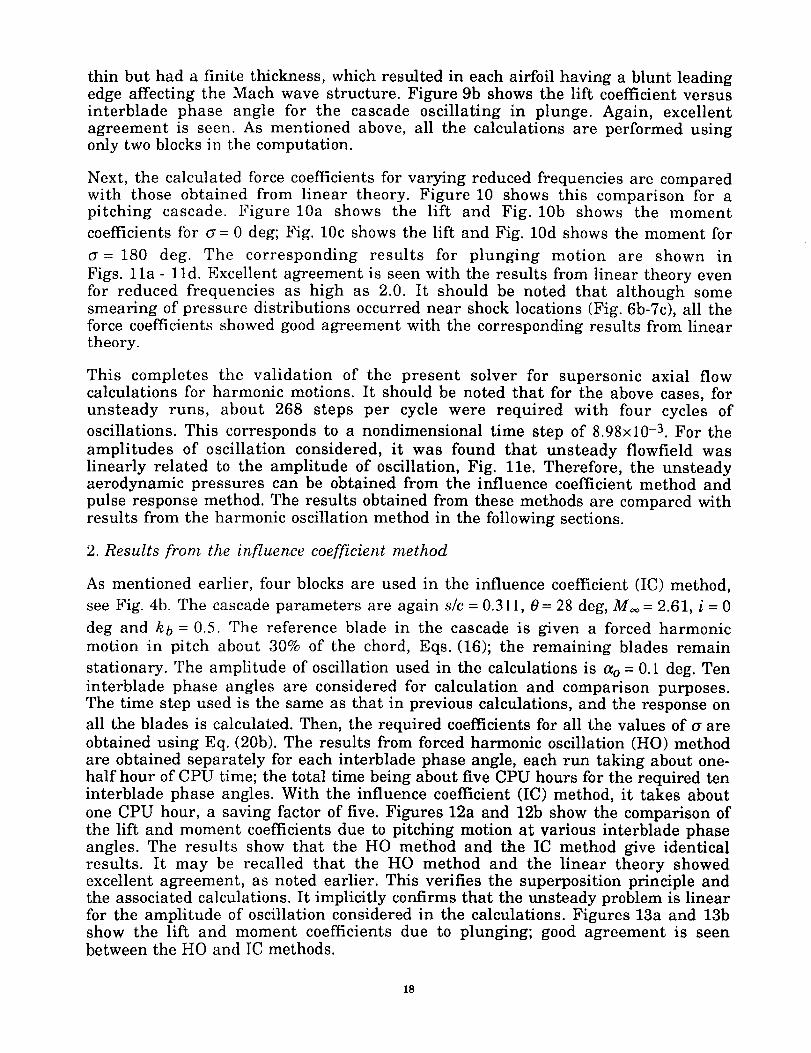
All the calculations are performed for the supersonic axial flow rotor (cascade)

geometry given in Ref. 8. The cascade has 58 blades (N=58), a gap-to-chord ratio (s/c)

of 0.311 and a stagger angle (0) of 28.0 deg. The inlet Mach number (M_)is 2.61. All of

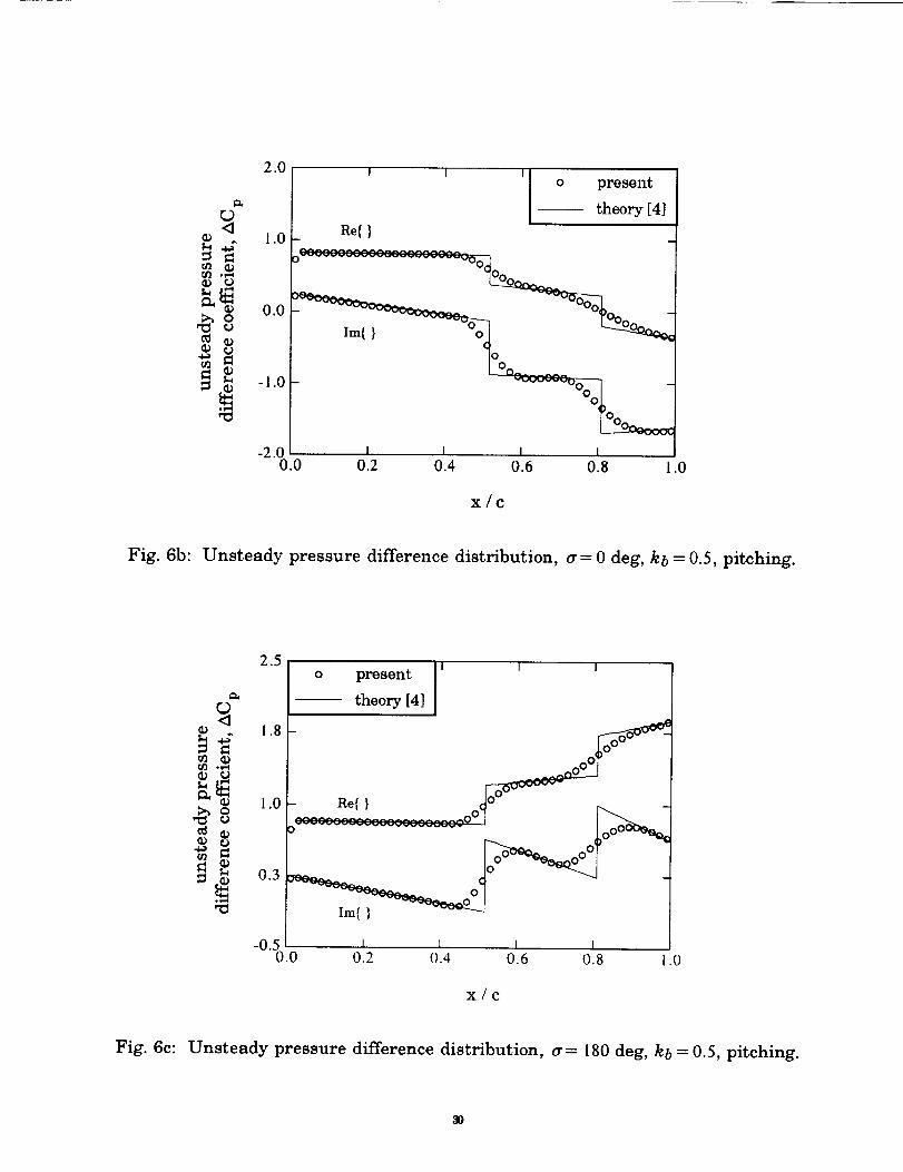
the Euler solutions are obtained using a H-grid for each passage. A typical grid is

shown in Fig. 2a for the rotor airfoil cascade and in Fig. 5 for the flat plate cascade. A

91x41 (streamwise by pitchwise) grid is used both for flat plate airfoils and rotor

airfoils; an algebraic grid generation scheme is used to generate this grid. The inlet

boundary is located only 0.3 chordlepgths upstream from the leading edge because,in supersonic axial flow, no disturbance can travel upstream from the leading edgeof the airfoil. There are 20 points in the streamwise direction in the region between

the inlet boundary and the leading edge. There are 50 points along each surface of the

airfoil, and 21 points beyond the trailing edge. The time step has been varied to check

its effect on convergence and accuracy. The calculations have been performed on a

Cray Y-MP computer. The solver takes about 5x10 -5 CPU seconds per time step per

grid point per block.

Code Validation

1. Results from the forced harmonic method

16

A cascade of flat plate airfoils is considered. The incidence angle (i)is 0 deg. The

reduced frequency based on semi-chord (kb) is 0.5 The cascade is oscillated in pitch

about the 30% of chord location, with an amplitude of oscillation (ao) of 0.1 deg. The

equations are time marched for a given interblade phase angle, until a periodicsolution is obtained. Four cycles of oscillation were found to be sufficient for the

solutions to become periodic in time as shown in Fig. 6a. The results from the last

cycle are Fourier decomposed to obtain the real and imaginary quantities.

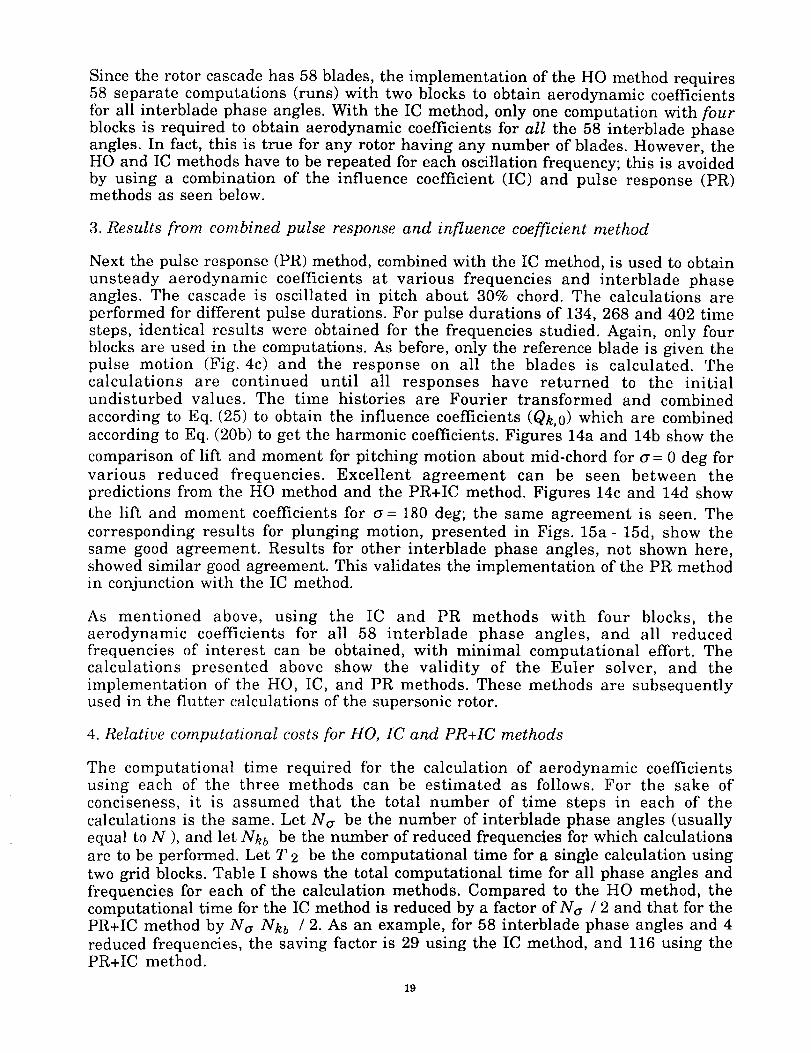
Figs. 6b and 6c show the predicted unsteady pressure distributions (first harmonic

pressure difference coefficient, ACp, versus chord) for _ = 0 and 180 deg, respectively.

These interblade phase angles require a minimum of one, and two grid blocks for

numerical calculations, respectively. The results from linear theory (Ref. 4) are also

plotted for comparison. For flat plate airfoils and small amplitudes of oscillation, the

present calculations are expected to agree with the linear theory of Ref. 4. The resultsfor the two interblade phase angles are in good agreement with those of Ref. 4. Note

that some smearing of the pressure distribution occurs near the reflected Mach wave

locations; however, the computed ACp's pass through the mid-point of the high andlow values of pressure at the discontinuity. Figure 6d shows the Mach contour lines

predicted by the present solver. The locations at which the Mach waves strike the

airfoil (x/c = 0.52 on the upper surface and x/c = 0.81 on the upper surface) comparewell with the locations given by linear theory.

Results are now presented for the flat plate cascade undergoing plunging motions;

these results are compared with results from linear theory. The amplitude of

oscillation is, ho/c = 3×10 -4 . The time response of lift coefficient is shown in Fig. 7a,

indicating that the response has become periodic. Figures 7b and 7c show pressure

distribution comparisons for (_= 0 and 180 deg, respectively. As for the pitching

motion cases, the agreement between the Euler predictions and linear theory is good.

These comparisons validate the present Euler solver for the two interblade phaseangles.

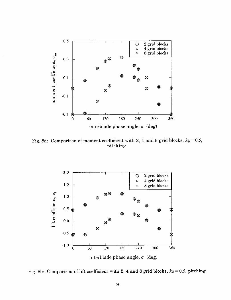
It was mentioned earlier that two blocks are sufficient for calculations at anyinterblade phase angle in supersonic axial flow. To verify this, calculations are

performed using two block, four block, and eight block configurations for ten

interblade phase angles. It should be noted here that two blocks represent (_ = 0 and

180 deg exactly; four blocks represent a = 0, 90, 180, 270 deg exactly; and eight blocks

represent (_ = 0, 45, 90, 135, 180, 225,270, 315 deg exactly. Figure 8a shows the plot of

moment coefficient versus interblade phase angle. The cascade is pitching about 30%

chord. It can be seen that all the three configurations give the same value indicatingthat for the supersonic axial flow solution, two blocks are sufficient to obtain

coefficients for any interblade phase angle. Similar comparison for lift coefficient is

shown in Fig. 8b. Results for plunging motion, not presented here, show the sametrend.

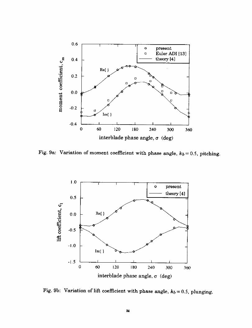
The variation of moment coefficient with interblade phase angle is compared with

that obtained from the linear theory of Ref. 4, and from the ADI-Euler analysis of

Ref. 13 in Fig. 9a. The cascade is pitching about 30% chord. Excellent agreement isseen with linear theory results. The discrepancy with those of Ref. 13 may be due to

the fact that the flat plate airfoil used in the calculations of Ref. 13 was not infinitely

17

thin but had a finite thickness, which resulted in each airfoil having a blunt leading

edge affecting the Mach wave structure. Figure 9b shows the lift coefficient versus

interblade phase angle for the cascade oscillating in plunge. Again, excellent

agreement is seen. As mentioned above, all the calculations are performed usingonly two blocks in the computation.

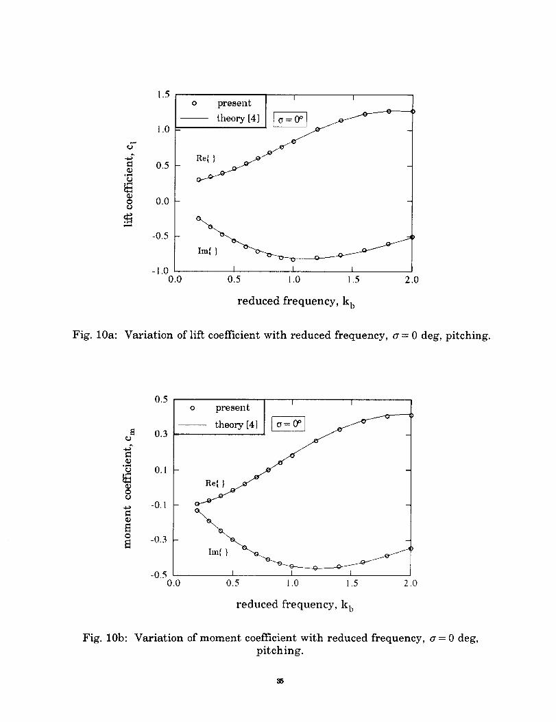
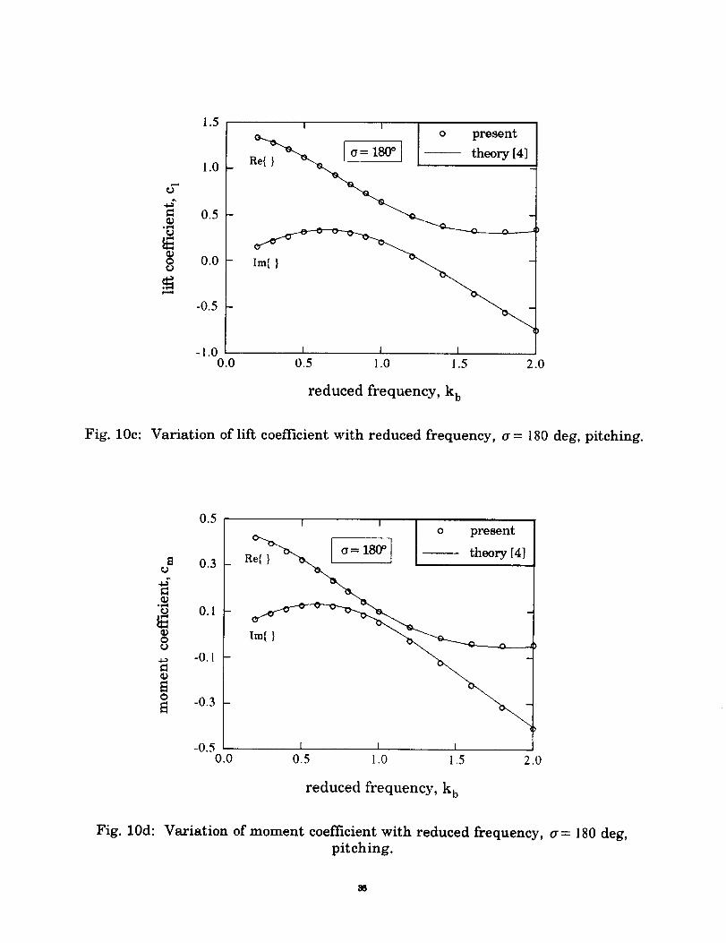
Next, the calculated force coefficients for varying reduced frequencies are compared

with those obtained from linear theory. Figure 10 shows this comparison for apitching cascade. Figure 10a shows the lift and Fig. 10b shows the moment

coefficients for _ = 0 deg; Fig. 10c shows the lift and Fig. 10d shows the moment for

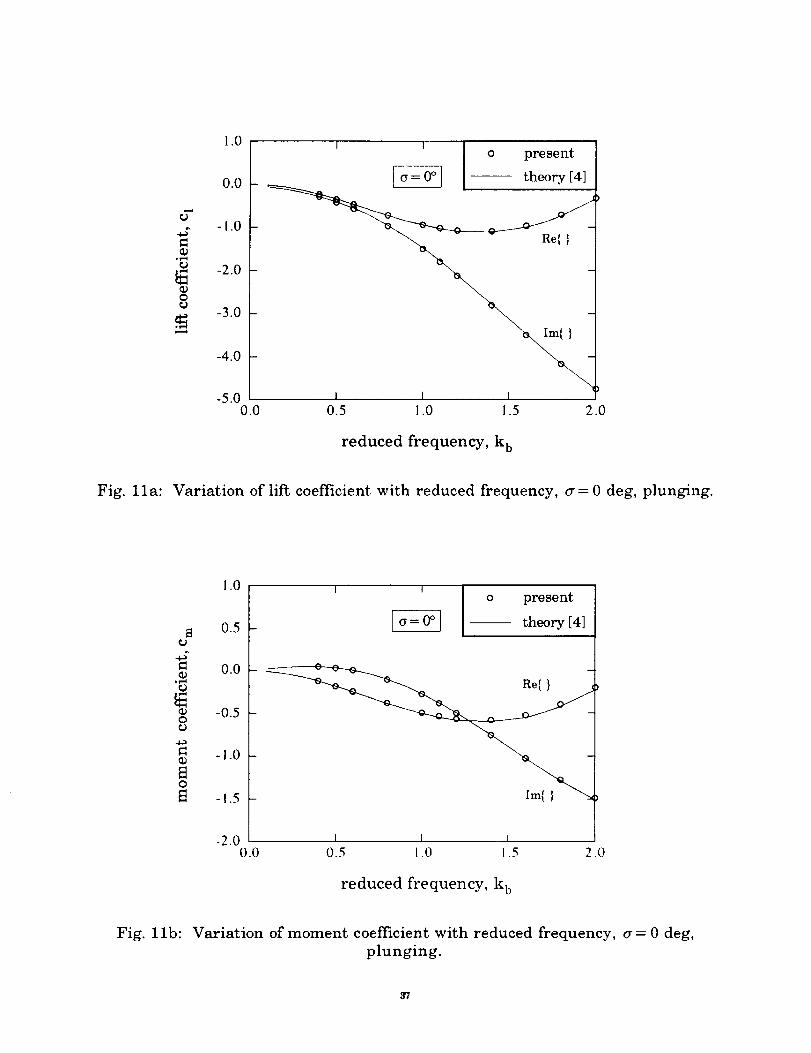
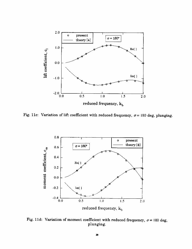
= 180 deg. The corresponding results for plunging motion are shown in

Figs. lla - lld. Excellent agreement is seen with the results from linear theory evenfor reduced frequencies as high as 2.0. It should be noted that although some

smearing of pressure distributions occurred near shock locations (Fig. 6b-7c), all the

force coefficients showed good agreement with the corresponding results from lineartheory.

This completes the validation of the present solver for supersonic axial flow

calculations for harmonic motions. It should be noted that for the above cases, for

unsteady runs, about 268 steps per cycle were required with four cycles of

oscillations. This corresponds to a nondimensional time step of 8.98x10 -3. For the

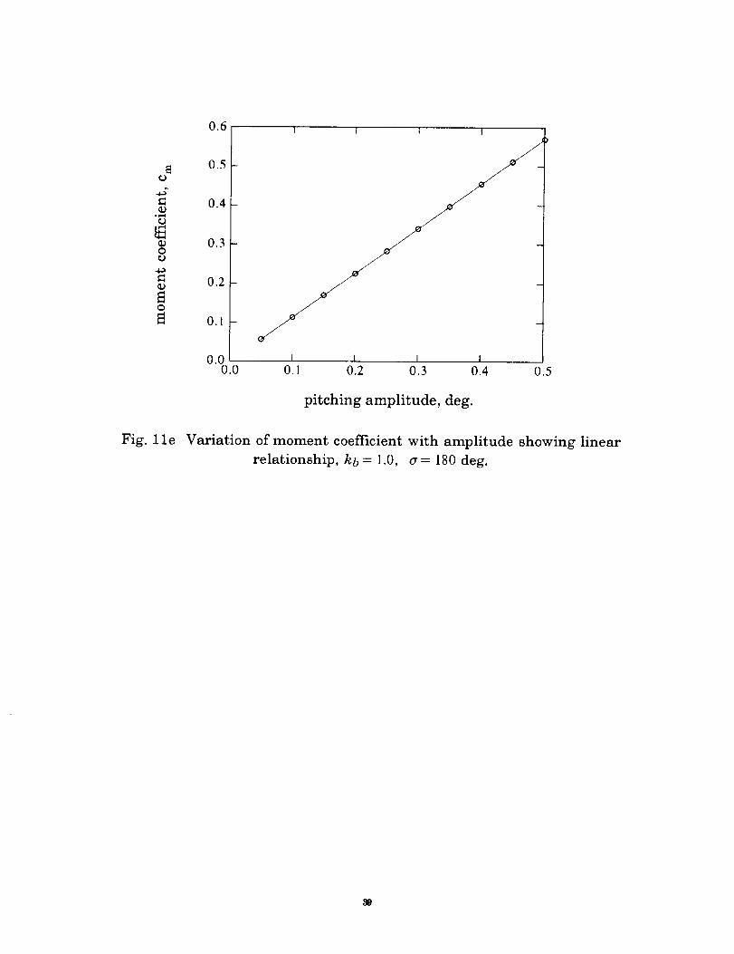
amplitudes of oscillation considered, it was found that unsteady flowfield was

linearly related to the amplitude of oscillation, Fig. lle. Therefore, the unsteadyaerodynamic pressures can be obtained from the influence coefficient method and

pulse response method. The results obtained from these methods are compared with

results from the harmonic oscillation method in the following sections.

2. Results from the influence coefficient method

As mentioned earlier, four blocks are used in the influence coefficient (IC) method,

see Fig. 4b. The cascade parameters are again s/c = 0.311, 0 = 28 deg, M_ = 2.61, i = 0

deg and kb = 0.5. The reference blade in the cascade is given a forced harmonic

motion in pitch about 30% of the chord, Eqs. (16); the remaining blades remain

stationary. The amplitude of oscillation used in the calculations is ao = 0.1 deg. Ten

interblade phase angles are considered for calculation and comparison purposes.

The time step used is the same as that in previous calculations, and the response on

all the blades is calculated. Then, the required coefficients for all the values of cr are

obtained using Eq. (20b). The results from forced harmonic oscillation (HO) method

are obtained separately for each interblade phase angle, each run taking about one-

half hour of CPU time; the total time being about five CPU hours for the required teninterblade phase angles. With the influence coefficient (IC) method, it takes about

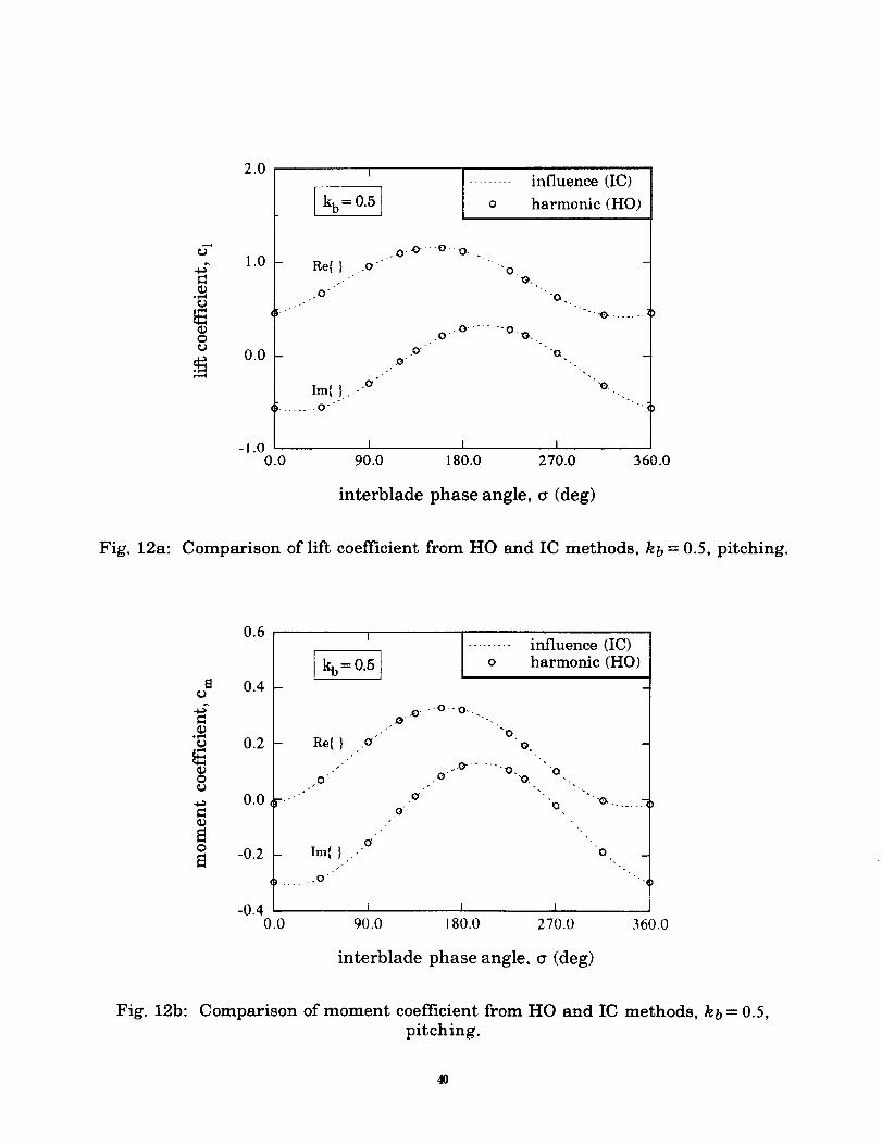
one CPU hour, a saving factor of five. Figures 12a and 12b show the comparison of

the lift and moment coefficients due to pitching motion at various interblade phaseangles. The results show that the HO method and the IC method give identical

results. It may be recalled that the HO method and the linear theory showed

excellent agreement, as noted earlier. This verifies the superposition principle andthe associated calculations. It implicitly confirms that the unsteady problem is linear

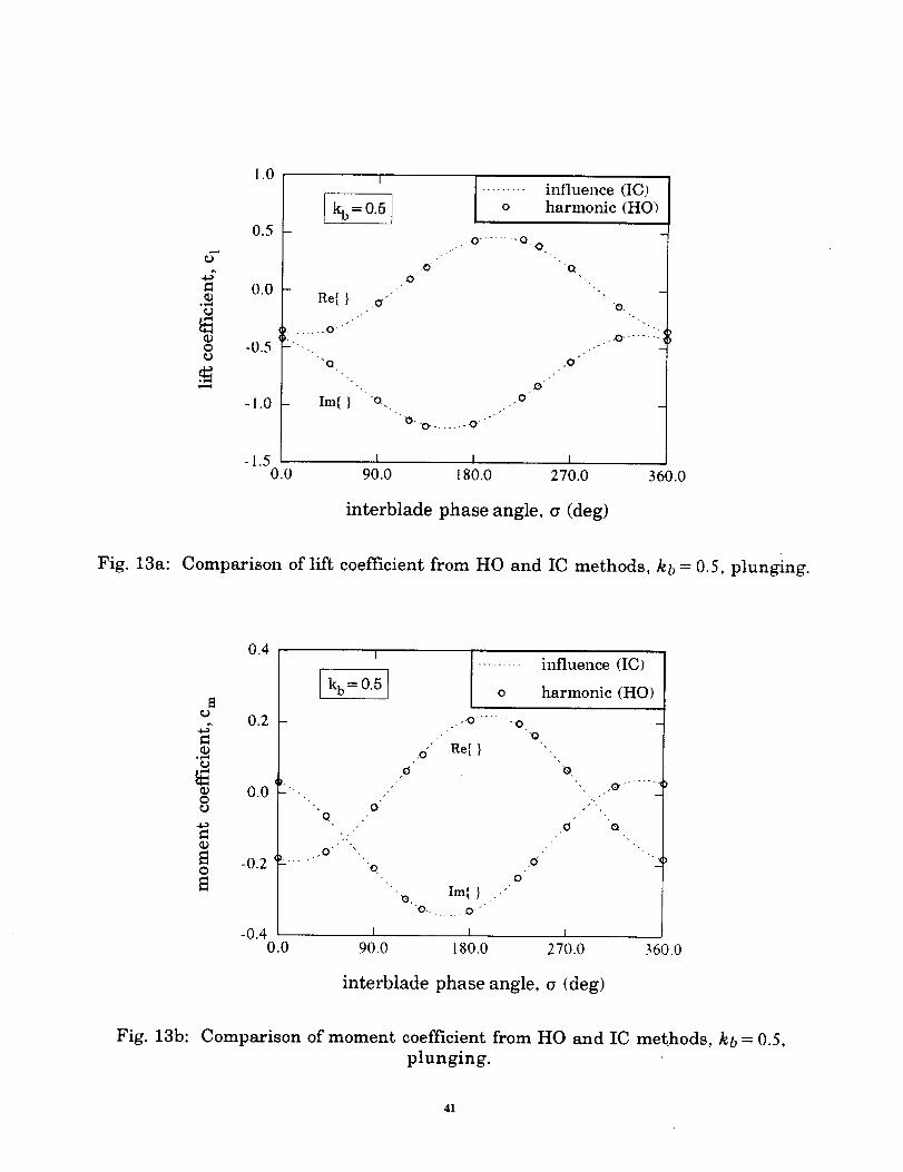
for the amplitude of oscillation considered in the calculations. Figures 13a and 13b

show the lift and moment coefficients due to plunging; good agreement is seenbetween the HO and IC methods.

18

Since the rotor cascade has 58 blades, the implementation of the HO method requires58 separate computations (runs) with two blocks to obtain aerodynamic coefficients

for all interblade phase angles. With the IC method, only one computation with fourblocks is required to obtain aerodynamic coefficients for all the 58 interblade phase

angles. In fact, this is true for any rotor having any number of blades. However, theHO and IC methods have to be repeated for each oscillation frequency; this is avoided

by using a combination of the influence coefficient (IC) and pulse response (PR)methods as seen below.

3. Results from combined pulse response and influence coefficient method

Next the pulse response (PR) method, combined with the IC method, is used to obtain

unsteady aerodynamic coefficients at various frequencies and interblade phaseangles. The cascade is oscillated in pitch about 30% chord. The calculations are

performed for different pulse durations. For pulse durations of 134, 268 and 402 time

steps, identical results were obtained for the frequencies studied. Again, only four

blocks are used in the computations. As before, only the reference blade is given thepulse motion (Fig. 4c) and the response on all the blades is calculated. The

calculations are continued until all responses have returned to the initial

undisturbed values. The time histories are Fourier transformed and combined

according to Eq. (25) to obtain the influence coefficients (Qk, o) which are combined

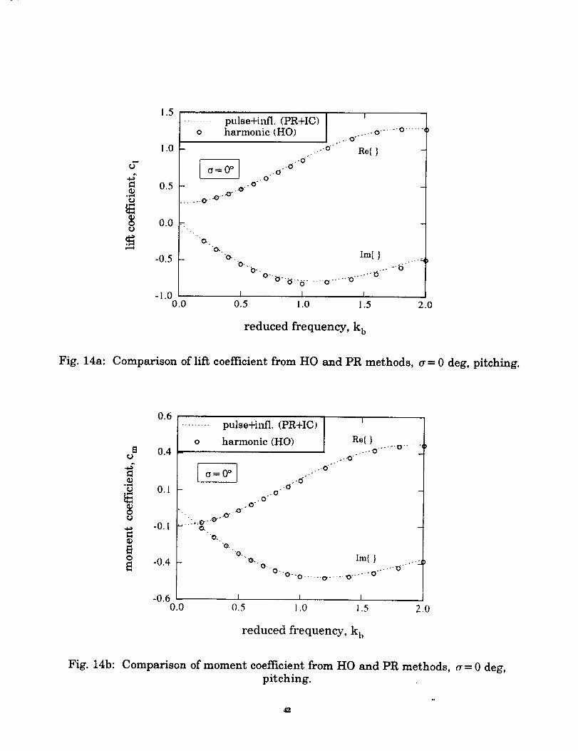
according to Eq. (20b) to get the harmonic coefficients. Figures 14a and 14b show the

comparison of lift and moment for pitching motion about mid-chord for (_ = 0 deg for

various reduced frequencies. Excellent agreement can be seen between the

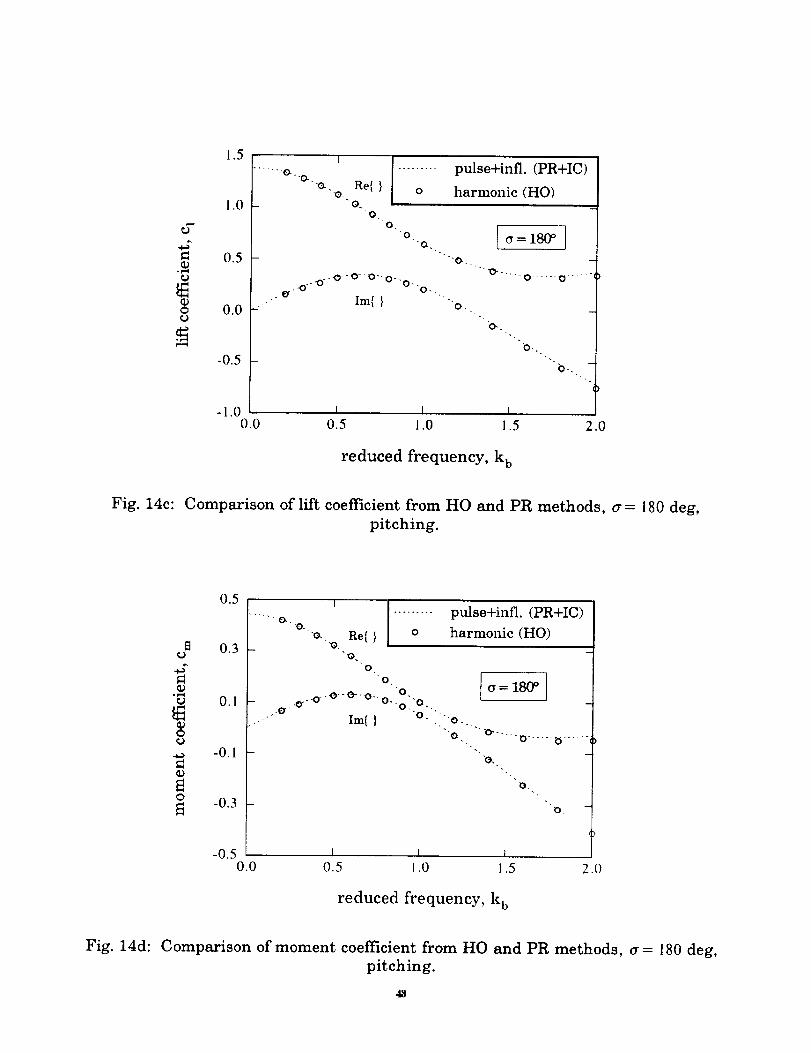
predictions from the HO method and the PR+IC method. Figures 14c and 14d show

the lift and moment coefficients for (_= 180 deg; the same agreement is seen. The

corresponding results for plunging motion, presented in Figs. 15a- 15d, show the

same good agreement. Results for other interblade phase angles, not shown here,

showed similar good agreement. This validates the implementation of the PR methodin conjunction with the IC method.

As mentioned above, using the IC and PR methods with four blocks, the

aerodynamic coefficients for all 58 interblade phase angles, and all reducedfrequencies of interest can be obtained, with minimal computational effort. The

calculations presented above show the validity of the Euler solver, and the

implementation of the HO, IC, and PR methods. These methods are subsequently

used in the flutter calculations of the supersonic rotor.

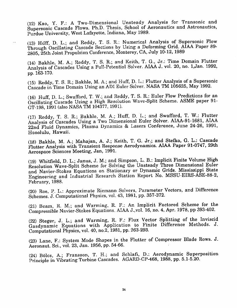
4. Relative computational costs for HO, IC and PR+IC methods

The computational time required for the calculation of aerodynamic coefficientsusing each of the three methods can be estimated as follows. For the sake of

conciseness, it is assumed that the total number of time steps in each of the

calculations is the same. Let Na be the number of interblade phase angles (usually

equal to N ), and let Nkb be the number of reduced frequencies for which calculations

are to be performed. Let T 2 be the computational time for a single calculation using

two grid blocks. Table I shows the total computational time for all phase angles and

frequencies for each of the calculation methods. Compared to the HO method, the

computational time for the IC method is reduced by a factor of Na / 2 and that for the

PR+IC method by Na Nkb / 2. As an example, for 58 interblade phase angles and 4

reduced frequencies, the saving factor is 29 using the IC method, and 116 using thePR+IC method.

19

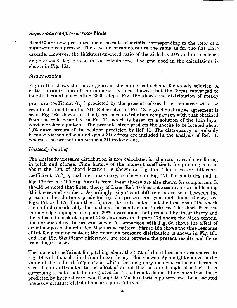
Supersonic compressor rotor blade

Resultg are now presented for a cascade of airfoils, corresponding to the rotor of a

supersonic compressor. The cascade parameters are the same as for the flat plate

cascade. However, the thickness-to-chord ratio of the airfoil is 0.05 and an incidence

angle of i = 8 deg is used in the calculations. The grid used in the calculations is

shown in Fig. 16a.

Steady loading

Figure 16b shows the convergence of the numerical scheme for steady solution. A

critical examination of the numerical values showed that the forces converged to

fourth decimal place after 2500 steps. Fig. 16c shows the distribution of steady

pressure coefficient (Cp) predicted by the present solver. It is compared with the

results obtained from the ADI-Euler solver of Ref. 13. A good qualitative agreement is

seen. Fig. 16d shows the steady pressure distribution comparison with that obtained

from the code described in Ref. 11, which is based on a solution of the thin layerNavier-Stokes equations. The present solver predicts the shocks to be located about

10% down stream of the position predicted by Ref. 11. The discrepancy is probablybecause viscous effects and quasi-3D effects are included in the analysis of Ref. 11,whereas the present analysis is a 2D inviscid one.

Unsteady loading

The unsteady pressure distribution is now calculated for the rotor cascade oscillating

in pitch and plunge. Time history of the moment coefficient, for pitching motion

about the 30% of chord location, is shown in Fig. 17a. The pressure difference

coefficient (ACp), real and imaginary, is shown in Fig. 17b for a= 0 deg and in

Fig. 17c for _= 180 deg. Results from linear theory are also shown for comparison. It

should be noted that linear theory of Lane (Ref. 4) does not account for airfoil loading

(thickness-and camber). Accordingly, significant differences are seen between the

pressure distributions predicted by the present analysis and linear theory; seeFigs. 17b and 17c. From these figures, it can be noted that the locations of the shockare shifted considerably due to the airfoil camber and thickness. The shock from the

leading edge impinges at a point 20% upstream of that predicted by linear theory andthe reflected shock at a point 20% downstream. Figure 17d shows the Mach contour

lines predicted by the present solver. A comparison with Fig. 6d shows the effect of

airfoil shape on the reflected Mach wave pattern. Figure 18a shows the time response

of lift for plunging motion; the unsteady pressure distribution is shown in Fig. 18band Fig. 18c. Significant differences are seen between the present results and thosefrom linear theory.

The moment coefficient for pitching about the 30% of chord location is compared inFig. 19 with that obtained from linear theory. This shows only a slight change in the

value of the reduced frequency at which the imaginary moment coefficient becomes

zero. This is attributed to the effect of airfoil thickness and angle of attack. It is

surprising to note that the integrated force coefficients do not differ much from those

predicted by linear theory even though the Mach reflection pattern and the associated

unsteady pressure distributions are quite different.

2O

Figures 20a and 20b show the results obtained from the influence coefficient and

pulse response methods for the rotor airfoil. The results are compared with those

obtained from the forced harmonic oscillation method. The comparisons show that

even for airfoils with thickness and camber, the IC and PR methods give goodcorrelation with HO method.

Flutter Calculations

The example considered is a tuned compressor cascade with 58 blades. The

geometric and structural parameters correspond to the rotor configuration studied

above. The structural model for each blade is a typical section (pitching andplunging). The pitching axis position is at 30% chord. This location was found to be

critical for flutter in Ref. 8. The radius of gyration is ra = 0.588 and the elastic axis is

located at the center of mass (xa = 0); the ratio of natural frequencies in bending and

torsion is O)h/O)a = 0.567; the mass ratio is tt = 456.

The flutter calculations in frequency domain, (for a fixed Mach number) require an

inner loop on interblade phase angle, with an outer loop on reduced frequency. Using

the HO method, this can be done as follows. Starting with the steady flowfield, a value

of reduced frequency (kb) is selected and the airfoils are forced in plunging motion

with a specified interblade phase angle ((_) until the flowfield becomes periodic in

time. The lift and moment coefficients are calculated at each time step and stored;

these are later decomposed into Fourier components to obtain the frequency domain

aerodynamic coefficients. This procedure is repeated for pitching motion. In this wayall four frequency domain aerodynamic coefficients corresponding to the specified

values of reduced frequency and phase angle are determined. The eigenvalueproblem given by Eq. (15) is then solved. The real part of the eigenvalue determines

the stability; the system is stable for the selected values ofkb and (_if the real part of

both eigenvalues is negative. The preceding steps are repeated for the remaining

values of (_. For a cascade with 58 blades, flutter can occur at any of the value of

given by Eq. (12a). If the cascade is found to be stable at all interblade phase angles,

then a lower value of reduced frequency is selected. This is continued until the real

part of one of the eigenvalues changes sign; this defines the flutter condition.

With the successful implementation of the PR+IC method the unsteady aerodynamic

coefficients for different kb and all (_ can be calculated in a smaller amount of CPU

time. Only four blade passages are considered in the calculations. One of the blades

is given a pulse, and the responses are recorded as mentioned earlier. Then using

the PR+IC method, the coefficients are calculated for each frequency and for each

phase angle as shown before, with considerable reduction in CPU time. The flutter

stability calculations are verified by performing calculations for a flat plate cascade.

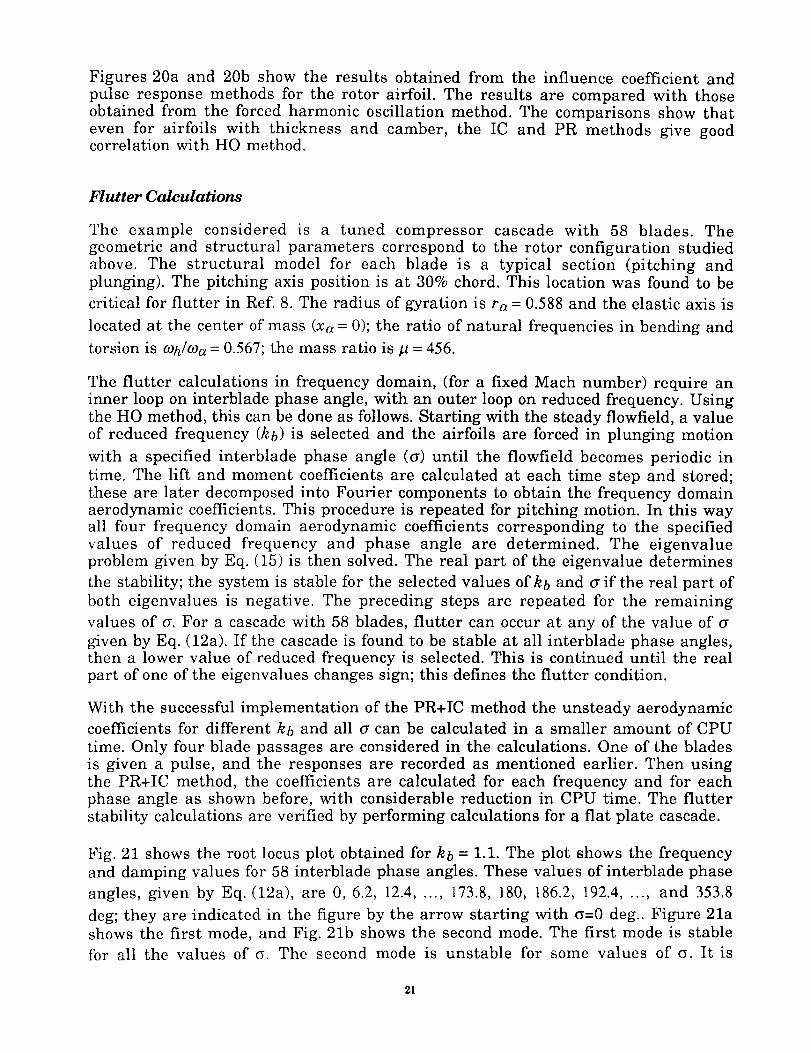
Fig. 21 shows the root locus plot obtained for kb = 1.1. The plot shows the frequency

and damping values for 58 interblade phase angles. These values of interblade phase

angles, given by Eq. (12a), are 0, 6.2, 12.4, ..., 173.8, 180, 186.2, 192.4, ..., and 353.8

deg; they are indicated in the figure by the arrow starting with (_=0 deg.. Figure 21a

shows the first mode, and Fig. 21b shows the second mode. The first mode is stable

for all the values of (_. The second mode is unstable for some values of g. It is

21

interesting to note that the damping values for the first mode are really one order less

than for the second mode, even though the first mode damping values are always

negative. The figures also show the comparison with the root locus plot obtained

from linear theory. Excellent agreement is seen, validating the IC, PR methods, theflutter calculations, and the present Euler aeroelastic solver.

Next, the calculations are repeated for the rotor airfoil cascade for kb = 1.1. The root

locus plot is shown in Fig. 22. As before, the first mode (Fig. 22a) is more stable than

the second mode (Fig. 22b). However, the following differences between the flat plate

and rotor airfoil results are noted. For the first mode (Fig. 22a), the area enclosed bythe root locus plot is more for the rotor as compared to the flat plate. The area

enveloped is determined by the spread in the frequency and damping due to

interblade coupling (cascade effects). Hence, Fig. 22a indicates that there is more

cascade effects for the rotor configuration. Further, the values of damping are

different for the rotor airfoil and flat plate for the same c. For the second mode

(Fig. 22b), the area enveloped by the root locus plot is nearly the same for both the flat

plate and rotor airfoils; however, the orientation of the plot is changed. Also the

eigenvalues show an opposite trend in relation to the order of increasing v. The

physical significance of these differences is not clear, except that they are due to theeffect of steady loading due to thickness and camber.

For the rotor airfoil cascade, calculations are repeated for different values of reduced

frequency until the real part of the eigenvalue changes sign. The phase angle at

flutter is _ = 192.4 deg, the frequency ratio is w/aJa = 1.002 and the reduced frequency

is kb = 1.09. The corresponding results for the flat plate cascade are _= 185.2 deg,

o)/o) a = 1.002 and kb = I. 153. This indicates that there is a marginal effect of airfoil

shape on stability.

CONCLUSIONS

Aeroelastic stability (flutter) analysis methods using an Euler solver have been

presented for supersonic axial flow cascades. The Euler solver is based on a flux

difference split algorithm. Results presented have shown the validity of the unsteadyEuler solver for harmonic blade oscillations, both in pitching and plunging motions.For harmonic oscillations, where the amplitude of oscillation is within the linear

range, influence coefficient and pulse response methods have been developed. These

methods have been successfully implemented and are shown to give same values of

the aerodynamic coefficients as obtained from harmonic oscillation method. These

methods considerably reduced the computational time for obtaining the aerodynamic

coefficients required in a frequency domain based flutter analysis. It has been shown

that a single calculation using four blade passages is enough to obtain the force

coefficients for any interblade phase angle and frequency of interest, irrespective ofthe number of blades in the cascade.

A two-degrees-of-freedom typical section model has been used for each blade of thecascade for flutter prediction. Each blade in the cascade has pitching and plunging

motions. Representative results from a frequency domain flutter analysis have been

obtained for a flat plate and for a rotor cascade configuration. Flutter results for the

selected structural parameters of the case studied indicated that the airfoil shape has

22

marginal effect on stability. In part II, flutter boundaries for a cascade of stator blade

airfoils are presented for various values of structural and geometric parameters.Such a parametric study will allow general conclusions to be drawn about the effectof airfoil shape on aeroelastic stability of supersonic flow cascades.

ACKNOWLEDGEMENTS

The authors acknowledge Mr. John Ramsey for providing the linear theory program.This work was supported by NASA grants NAG3-1137, NAG3-1234, and NAG3-983.

_CF_

(1) Strack, W. C.; and Morris Jr., S. J.: The Challenges and Opportunities ofSupersonic Transport Propulsion Technology. NASA TM 100921, 1988.

(2) Wood, J. R. et al: Application of Advanced Computational Codes in the Design of

an Experiment for a Supersonic Throughflow Fan rotor. ASME Paper 87-GT-160.

(3) Ball, C. L.: Advanced Technologies Impact on Compressor Design and

Development: A Perspective. NASA TM 102341, presented at Aerotech '89, Society ofAutomative Engineers, Anaheim, CA, Sept. 25-28, 1989.

(4) Lane, F.: Supersonic Flow Past an Oscillating Cascade with SupersonicLeading- Edge Locus. J. of Aeronaut. Sci., vol. 24, 1957, pp. 65-66.

(5) Platzer, M. F.; and Chalkley, Lt. H. G.: Theoretical Investigation of SupersonicCascade Flutter and Related Interference Problems. AIAA Paper 72-377, 1972.

(6) Nishiyama, T.; and Kikuchi, M.: Theoretical Analysis for UnsteadyCharacteristics of Oscillating Cascade Aerofoils in Supersonic Flows. The

Technology Reports of the Tohoku University, vol. 38, no. 2, 1973, pp 565-597.

(7) Nagashima, T.; and Whitehead, D. S.: Linearized Supersonic Unsteady Flow inCascades. British ARC R & M 3811, 1977.

(8) Kielb, R. E.; and Ramsey, J. K.: Flutter of a Fan Blade in Supersonic Axial Flow.J. Turbomach., vol. 111, no.4, October 1989, pp. 462-467.

(9) Kaza, K. R. V.; and Kielb, R. E.: Flutter and Response of a Mistuned Cascade in

Incompressible Flow. AIAA J., vol. 20, no. 8, Aug. 1982, pp. 1120-1127.

(10) Ramsey, J. K.: Influence of Thickness and Camber on the Aeroelastic Stability

of Supersonic Throughflow Fans. J. Propulsion and Power, vol. 7, no. 3, May-June,1991, pp. 404-411.

(11) Chima, R. V.: Explicit Multigrid Algorithm for Quasi-Three Dimensional

Viscous Flows in Turbomachinery. J. of Propulsion and Power, vol. 3, no. 5, Sept-Oct. 1987, pp 397-405.

23

(12) Kao, Y. F.: A Two-Dimensional Unsteady Analysis for Transonic and

Supersonic Cascade Flows. Ph.D. Thesis, School of Aeronautics and Astronautics,

Purdue University, West Lafayette, Indiana, May 1989.

(13) Hffff, D. L.; and Reddy, T. S. R.: Numerical Analysis of Supersonic Flow

Through Oscillating Cascade Sections by Using a Deforming Grid. AIAA Paper 89-

2805, 25th Joint Propulsion Conference, Monterey, CA, July 10-12, 1989

(14) Bakhle, M. A.; Reddy, T. S. R.; and Keith, T. G., Jr.: Time Domain Flutter

Analysis of Cascades Using a Full-Potential Solver. AIAA J. vol. 20, no. 1,Jan. 1992,

pp. 163-170.

(15) Reddy, T. S. R.; Bakhle, M. A.; and Huff, D. L.: Flutter Analysis of a Supersonic

Cascade in Time Domain Using an ADI Euler Solver. NASA TM 105625, May 1992.

(16) Huff, D. L.; Swafford, T. W.; and Reddy, T. S. R.: Euler Flow Predictions for an

Oscillating Cascade Using a High Resolution Wave-Split Scheme. ASME paper 91-

GT-198, 1991 (also NASA TM 104377, 1991).

(17) Reddy, T. S. R.; Bakhle, M. A.; Huff, D. L.; and Swafford, T. W.: Flutter

Analysis of Cascades Using a Two Dimensional Euler Solver. AIAA-91-1681, AIAA

22nd Fluid Dynamics, Plasma Dynamics & Lasers Conference, June 24-26, 1991,

Honolulu, Hawaii.

(18) Bakhle, M. A.; Mahajan, A. J.; Keith, T. G. Jr.; and Stefko, G. L.: Cascade

Flutter Analysis with Transient Response Aerodynamics. AIAA Paper 91-0747, 29th

Aerospace Sciences Meeting, Jan, 1991.

(19) Whitfield, D. L.; Janus, J. M.; and Simpson, L. B.: Implicit Finite Volume High

Resolution Wave-Split Scheme for Solving the Unsteady Three Dimensional Euler

and Navier-Stokes Equations on Stationary or Dynamic Grids. Mississippi State

Engineering and Industrial Research Station Report No. MSSU-EIRS-ASE-88-2,

February, 1988.

(20) Roe, P. L.: Approximate Riemann Solvers, Parameter Vectors, and Difference

Schemes. J. Computational Physics, vol. 43, 1981, pp. 357-372.

(21) Beam, R. M.; and Warming, R. F.: An Implicit Factored Scheme for the

Compressible Navier-Stokes Equations. AIAA J.,vol. 16, no. 4, Apr. 1978, pp 393-402.

(22) Steger, J. L.; and Warming, R. F.: Flux Vector Splitting of the Inviscid

Gasdynamic Equations with Application to Finite Difference Methods. J.

Computational Physics, vol. 40, no.2, 1981, pp. 263-293.

(23) Lane, F.: System Mode Shapes in the Flutter of Compressor Blade Rows. J.

Aeronaut. Sci., vol. 23, Jan. 1956, pp. 54-66.

(24) BSlcs, A.; Fransson, T. H.; and Schlafi, D.: Aerodynamic Superposition

Principle in Vibrating Turbine Cascades. AGARD-CP-468, 1988, pp. 5.1-5.20.

24

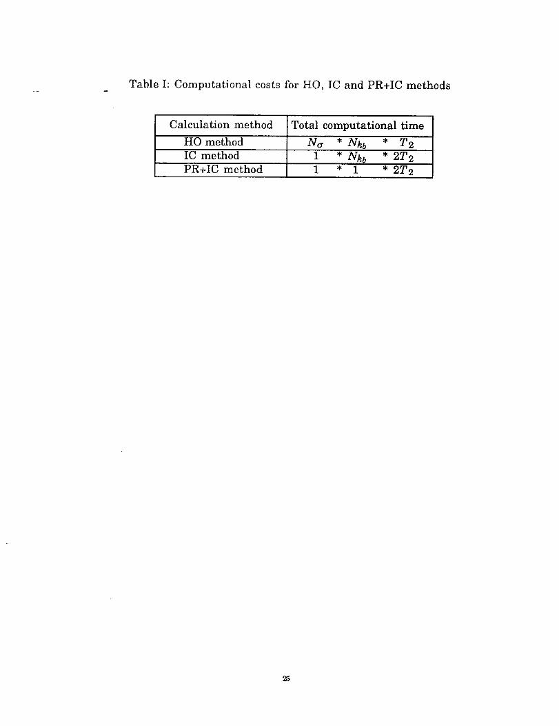
Table I: Computational costs for HO, IC and PR+IC methods

Calculation method Total computational time

HO method Na * Nkb * T2

IC method 1 * Nkb * 2T2

PR+IC method 1 * 1 * 2T2

25

b _I _

ofmass--_ _ [bah__ -

-- undeflected

r _ Qa l h airfoil position

_ elastic

axis

Figure 1: Typical section blade model with two degrees-of-freedom.

stagger

inlet line r--lower surface

/periodic / t periodic

E / boundary/F / G boundary H

£i'?;i!!?;6";;,_+';;""

,-f%eriodic /R-- " periodic /D

rY/[ Lboundaupper surface i C boundary/c_ chord line [

_ c _ exit

Figure 2a: Cascade geometry and grid for one blade passage.

stagger

inlet line r--lower surface

/periodic / t periodic

I/ boundary/J t K boundary L

E H

Aeriodic - -: -r /ff_t-upper surface i _ periodic

L-chord line I boundaryc _ exit

Figure 2b: Cascade geometry and grid for two blade passages.

/=,y

_=l .Ii=l

iIe ire

_[ .IV . V . VI / f deform

_Aj /J d_a /

-- VII ,m _ .4__ passageI centeriine

Y fix /

t, -| II III / I deform

ile ite _ ni

Figure 2c: Sub-blocking used for deforming the grid.

E-_

block 2

I / ! l/ . interior cells of & phantom cells of

/i//._F block 2 at jffi 2 block 1at jffi r_]+l- interior cells of & phantom cells of

block 1 block 1 at j= nj block 2 at j = 1

periodic periodic

boundary ---] boundary --7

I / J K / L

_ block2 '_====_ ' -- /

F'------- injection [

, /

block 1

2

_/ B c/Dperiodic periodic

bom,dao" bounda_"

Figure 2d: Periodic and injection boundaries used in calculations with multiple

grid blocks.

27

ref+l

Lshock lines7

ref

Fig. 3. Cascade in supersonic axial flow

ref+3

re f+2

ref+l

ref

ref-1

ref-2

ref-3

(a) Harmonic (b) Influence (c) Pulse

Oscillation (HO) Coefficient (IC) Response (PR)

Fig. 4: Setup showing number of blocks used in computation withblade motion as indicated.

28

leading edge trailing edge

Fig. 5: Flat plate grid (91,,41)

0.0015

0.0010

0.0005

0.00000

-0.0005

0

-o.oolo

I I 1 I I

U

-0.0015 I t I t I0 2 4 6 8 10 12

nondimensional time, r

Fig. 6a: Moment coefficient vs. time in pitching motion, kb = 0.5. rr= 180 deg.

ao = 0. I deg.

29

2.0

<1_ 1.0

_ 0.0

._. -1.0"o

-2.00.0

_ _[ o present

I-- theory [4]

Re{} ..N...

Oo

o

I I I 1

0.2 0.4 0.6 0.8 .0

x/c

Fig. 6b: Unsteady pressure difference distribution, a= 0 deg, kb = 0.5, pitching.

x/c

Fig. 6c: Unsteady pressure difference distribution, a= 180 deg, kb = 0.5, pitching.

30

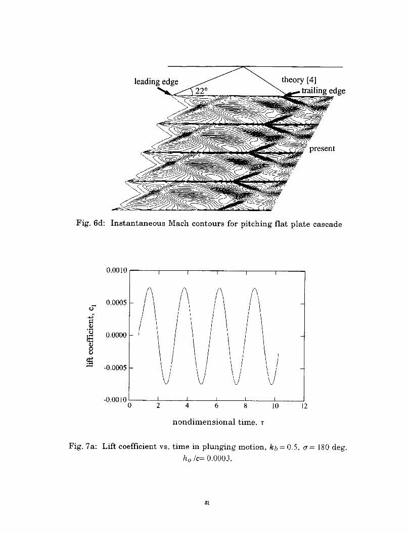
Fig. 6d:

plesent

Instantaneous Mach contours for pitching fiat plate cascade

u-

_9

_9

0.0010

0.0005

0.0000

-0.0005

I I I I I

-0.0010 I I I i i0 2 4 6 8 10 12

nondimensional time. r

Fig. 7a: Lift coefficient vs. time in plunging motion, kb = 0.5. G= 180 deg,

ho /c= 0.0003.

81

1.5

1.0

_ 0.5,el

rj

°.°-_ _ -0.5

•_ -1.0

I Io present,Re{ }

+ present,Im{ }theory [4],Re{ }

..... theory [4],Ira{}

- - _.;.,.-+_,,._t +

4. +............. OC_'O0"'_O°O I ++' -

O/ ++ ,

C_o-++-+,,4--_....

--I.5 J I J I

0.0 0.2 0.4 0.6 0.8 1.0

x/e

Fig. 7b: Unsteady pressure difference distribution, a= 0 deg, kb = 0.5, plunging.

c_ _j_J cJ

°_==1

2.0 I I I

o present Itheory [4]

70 o

Re{ } oL _ .... t_0.0 _.._c_..e ........... -..-,-,-- ' --J

-I.0

Im{} "[0-00-i"_e'v2Z'Z_--_O°O00J"_ 7'00,-,_ ]I I I -IL_-_-Oc_

0.2 0.4 0.6 0.8 I .0

x/c

Fig. 7c: Unsteady pressure difference distribution, a= 180 deg, kb = 0.5, plunging.

o

=09

09¢)

09

O

0.5

0.3

0.1

C

-0.1

I I I

®@ ®

L © 2 grid blocksc 4 grid blocks× 8 grid blocks

@ ® ®® ®

® @® ®

®®

-0.3 _ _l I I I I0 60 120 180 240 300 360

interblade phase angle, cr (deg)

Fig. 8a: Comparison of moment coefficient with 2, 4 and 8 grid blocks, kb = 0.5,

pitching.

2.0

1.5

1.0

09

0.509Oc9

o.o

-0.5

I I I

®® ®

O 2 grid blocks

[] 4 grid blocks

× 8 grid blocks

@ @@

@ @

® @@

®® @

® ®

-1.0 I I I I i0 60 120 180 240 300 360

interblade phase angle. (r (deg)

Fig. 8b: Comparison of lift coefficient with 2, 4 and 8 grid blocks, kb = 0.5, pitching.

0.6

t_ 0.4

0_.,-4 0.2

0

_ 0.0

0

-0.2

-0.4

i t i ' I o present

Etder ADI [13]

theory [4]

I I I I I I

0 60 120 180 240 300 360

interblade phase angle, cr (deg)

Fig. 9a: Variation of moment coefficient with phase angle, kb = 0.5, pitching.

o-

O¢J

1.0

0.5

0.0

-0.5

-1.0

-1.5

'T T T

o presenttheory[4]

__l L 1 i.---------/

0 60 120 [80 240 300 360

interblade phase angle, cr (deg)

Fig. 9b: Variation of lift coefficient with phase angle, kb = 0.5, plunging.

84

C9

C9

_DO

1.5

1.0

0.5 --

0.0-

-0.5

-I.00.0

o present ] '

- theory [4] ] _-______

I

I t I

0.5 1.0 1.5 2.0

reduced frequency, k b

Fig. 10a: Variation of lift coefficient with reduced frequency, _= 0 deg, pitching.

0.5

t_ 0.3¢9

"_ 0.1

0

._ -0.1 -

0

-0.3 -

present [ 1 1

theory [4_

I I I

0.5 1.0 1,5 :.0

reduced frequency, k b

Fig. 10b: Variation of moment coefficient with reduced frequency, a = 0 deg,pitching.

_9

O

1.5

1.0

0.5

0.0

-0.5

-1.00.0

' ' I o present

I (_= 180 _ [ - theory [4]

Re{} _ ' L _ -" _ __

I I I

0.5 1.0 1.5 2.0

reduced frequency, k b

Fig. 10c: Variation of lift coefficient with reduced frequency, a= 180 deg, pitching.

0.5

gt 0.3

*1"_

_:_ 0.1

0e_

_ -0. I

0

-o.3

' ] o present

R_-- theory. [4]

I I 1-0.50.0 0.5 1.0 1.5 2.0

reduced frequency, k b

Fig. 10d: Variation of moment coefficient with reduced frequency, a = 180 deg,

pitching.

1.0

0.0

-I.0

°r"_

-2.0

0

-3.0

-4.0

-5.00.0

I I I o present I

_ _ Re[ } _

I I I

0.5 1.0 1.5 Z.O

reduced frequency, k b

Fig. 11a: Variation of lift coefficient with reduced frequency, a = 0 deg, plunging.

1.0

0.5

0.0

-0.5o

-1.0

o

a -I.5

i _ [ o present

_-_ ]_ theory [4]

Ira{}

I t I

0.5 1.0 1.5 :.0

reduced frequency, k b

Fig. 11b: Variation of moment coefficient with reduced frequency, a = 0 deg,plunging.

37

O--

or-¢

o_J

F===¢

2.0

1.0

0.0

-I.0 -

-2.00.0

o present I ' I'theory [4] a = 180 °

Ira{}

I I t0.5 1.0 1.5 2.0

reduced frequency, k b

Fig. 11c: Variation of lift coefficient with reduced frequency, cr = 180 deg, plunging.

O

(D00

0

o

0.8

0.6

0.4

0.2 --

0.0 -

-0.2 -

-0.40.0

J _ l o present

Io--l 1 l--

Re{ }

0.5 I .0 i .5 2.0

reduced frequency, k b

Fig. lld: Variation of moment coefficient with reduced frequency, or= 180 deg,

plunging.

88

_9

o,.._

_9OC9

q9

O

0.6

0.5

0.4

0.3

0.2-

0.1-

0.00.0

I I

I I I

0.1 0.2 0.3I

0.4 0.5

pitching amplitude, deg.

Fig. 11e Variation of moment coefficient with amplitude showing linear

relationship, kb = 1.0, a= 180 deg.

2.0

.- 1.0

.p,,I

0

o.o

-I.0

......... influence (IC)

o harmonic (HO)

., O..O .... O.-o..,

Re{ } .o" "o,

..0" "0..°

.0'

,o..O ........ O,o.,

"Ct

Ira{ )...-.o "o,

I I I

).0 90.0 180.0 270.0 360.0

interblade phase angle, o (deg)

Fig. 12a: Comparison of lift coefficient from HO and IC methods, kb = 0.5, pitching.

_9

o_

O

O

0.6

0.4 --

0.2-

0.0 .... "

-0.2

-0.40.(

Re{ } o

o

hn{ }.-

..... ..0"

......... influence (IC)o harmonic (HO)

O, O .... O'-O, ,

D,

,,O" ....... O, 'CtO" "O.

O' ' "O-. -O" Q "'"

'D

I I I

90.0 180.0 270.0 360.0

interblade phase angle, a (deg)

Fig. 12b: Comparison of moment coefficient from HO and IC methods, kb = 0.5,

pitching.

40

=_9

+_,,I

¢9

<PO

1.0

0.5

0.0

-0.5

-I.0

kb= 0.5

m

Re{ } .c'"

I: ....... O

"O

Irn{ } "0

0

......... influence (IC)o harmonic (HO)

..0 ........O 0

-0"

O- O- .......O" ""

0

.0

I I I

0

.0

-1.50.0 90.0 180.0 270.0 360.0

interblade phase angle, a (deg)

Fig. 13a: Comparison of lift coefficient from HO and IC methods, kb = 0.5, plunging.

0.4

C9 0.2

(D°t.-4

0.00U

-0.20

-0.4

"'.. ,"

O"0

.0"

0

I ......... influence (IC)o harmonic (HO)

., .-O ....... "O

.o" Re{ }

0

"e. Im{} ."

o. ......o"

I I

_.0 90.0 180.0

o

',, ,,Or"" .... "1• , m

O Q

2

I

270.0 360.0

interblade phase angle, o (deg)

Fig. 13b: Comparison of moment coefficient from HO and IC met.hods, kb = 0.5,

plunging.

41

C,v.._

¢J

_0O¢J

1.5

1.0

0.5

0.0

-0.5

-1.00.0

......... pulse+imCl. (PR+IC)o harmonic (HO)

.'5

I .-00"=0 ° ..O.O

,O"

...... O- -G-" _"

.... O ...... O .....

Re[ }

"'..

"O-. Im[ } ..... :_0.. ..-" b

b-.. ---'6"°' b"_"_5 ......o .0o-

I I I

0,5 1,0 1.5 2.0

reduced frequency, k b

Fig. 14a: Comparison of lift coefficient from HO and PR methods, q = 0 deg, pitching.

0.6

t_ 0.4

o_,-4

O.l

0

_ -0.1C

0

-0.4

-0.6

......... pulse+intl. (PR+IC) ]

Io harmonic (HO)

.0

=.i:,:e..-e'"O.

"Q.,

*O*

Re{ }....-0 ...... 0 ..... --(

...- "0"

Im(} .-"i

O- "0- "0 ...... 0 ..... 0 ...... 0""

I I I

_.0 0.5 1.0 1.5 2.0

reduced frequency, k b

Fig. 14b: Comparison of moment coefficient from HO and PR methods, a = 0 deg,pitching.

42

1.5 _ ......... pulse+intl. (PR+IC) I

""O.._. "'O Re{} o harmonic (HO) _ i

1.0 "°'.o.'0 "

u- "o- o I_=180 _

oooo ...........Er "-0"" "0 _ v, "0 -. |

-0.5

- 1.00. 0 0.5 1.0 1.5 2.0

reduced frequency, k b

Fig. 14c: Comparison of lift coefficient from HO and PR methods, a= 180 deg,pitching.

_9

_9O_9

_D

O

0.5 -

0.3

0.1

-0.5 _0.0

-O.l

-0.3

"'0-. 0"o, Re{ }

"O

"O,

"O''O'-_'O" O" °O "O,,,O'" • ".

Ira{]

pulse+intl. (PR+IC)

harmonic (HO)

Io=180° 1

"O. °"-O..

O ...... _ ......

.°

O.

I I I

0.5 1.0 1.5

reduced frequency, k b

..0

Fig. 14d: Comparison of moment coefficient from HO and PR methods, a = 180 deg,pitching.

4_

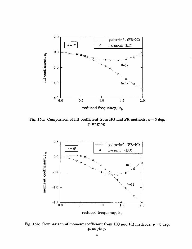
,r

a9

t9

2.0

0.0

-2.0

-4.0 -

-6.00.0

......... pulse+intl. (PR+IC)

o harmonic (HO)

@::@::0:: .... o--O.. .... O'-o-. O ..... "O'"

"Q

"QRe{}

O.

"'- m

Im{ } "o.

I I I0.5 1.0 1.5 2.0

reduced frequency, k b

Fig. 15a: Comparison of lift coefficient from HO and PR methods, a = 0 deg,

plunging.

_J

¢J

O

0.5

0.0

-0.5

-1.0 -

-1.50.0

--| t ......... pulse+intl. (PR+IC)

1 o harmonic (HO)

.,Q.. '0

"0.. -Q

"O..

"0-

Re{ }

'o, , .,-b

o::g,. -o"

'0,

-, Ira{}Q

l I 1

0.5 1.0 I .5 2.0

reduced frequency, k b

Fig. 15b: Comparison of moment coefficient from HO and PR methods, a = 0 deg,plunging.

44

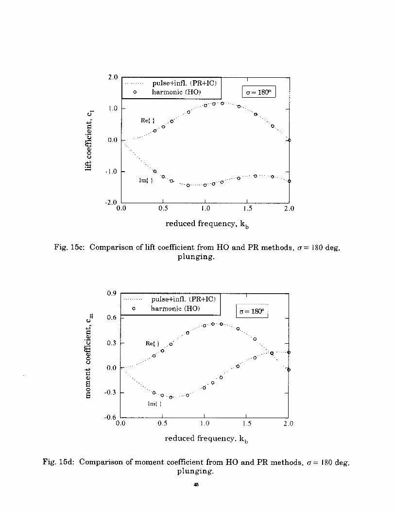
°_,,d

c_

O

i----d

2.0

1.0

0.0

-1.0

......... pulse+intl. (PR+IC)

o harmonic (HO)

Re{ }

.....-'"

"Q"Q.

Imp}

.O

,.O

I

..--0" 0-0 ......

O.

.... O...... _O...... O ...."Q-. 0..0- --_-'0 ..... 0

-2.0 l I J0.0 0.5 1.0 1.5 2.0

reduced frequency, k b

Fig. 15c: Comparison of lift coefficient from HO and PR methods, a= 180 deg,

plunging.

0.9

0.6

• r,,,,I

0.3

0

_ 0.0

0

-0.3

......... pulse+intl. (PR+IC)

o harmonic (HO)

.-"'0" .0--0-..

.O

." "0

Re( } .0" " -,.0' -•'--:0 .....

,o" .-0 ,,

.0

- "O"O'O- -Q"

Im{l

-0.6 ± J I0.0 0.5 1.0 1.5 2.0

reduced frequency, k b

Fig. 15d: Comparison of moment coefficient from HO and PR methods, a= 180 deg,

plunging.

45

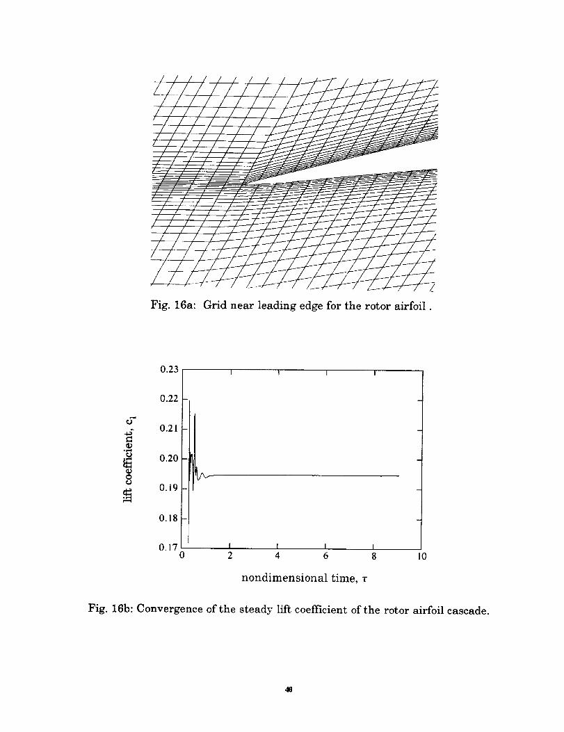
if-f�-�

//

/I/ /.i

/J

/ ,/

/ 7-7

• / /

Fig. 16a: Grid near leading edge for the rotor airfoil.

o-

.,--I

g¢9

0.23

0.22

0.21

0.20

0.19

0.18

I I I I

m

n

m

0.17 I i i j0 2 4 6 8

nondimensional time, r

lO

Fig. 16b: Convergence of the steady lift coefficient of the rotor airfoil cascade.

48

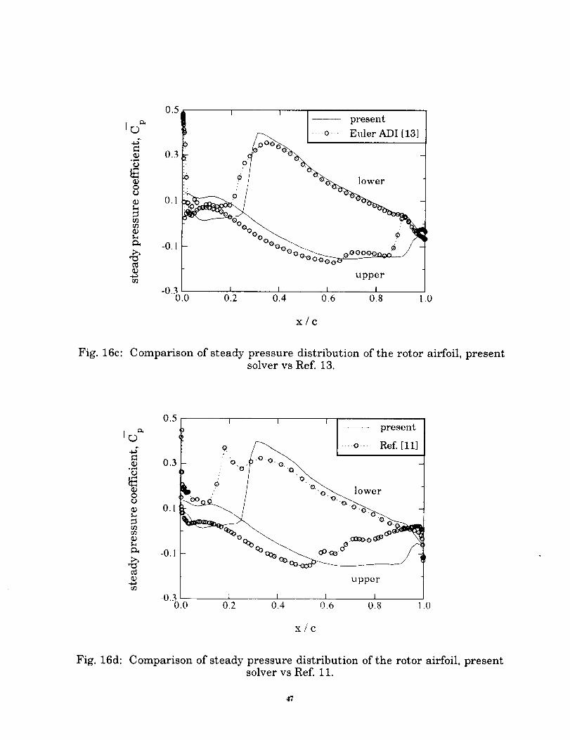
I_ _

o_..4

C9

_9O_9

_9

_D

_9

O9

O_

0.5

0.3

0.1

-0.1

-0.30.0

I I

present

:_L: Eu]e___[rAD__ I[ a__11

! 0 ,'0 / __ lower

upper

I I I I

0.2 0.4 0.6 0.8 .0

x/c

Fig. 16c: Comparison of steady pressure distribution of the rotor airfoil, presentsolver vs Ref. 13.

°1-.4_9

_DOC9

O9

O9

O0

0.5

o_

0.3 .

0.1 _

-0.1

-0.3 J0.0 0.2

, , i [ present]

'o )- -- - v. o, ._"o" 0.o

lower

-_ -

"_%._ oo_.

upper

] 1 I

0.4 0.6 0.8 .0

x/c

Fig. 16d: Comparison of steady pressure distribution of the rotor airfoil, presentsolver vs Ref. 11.

47

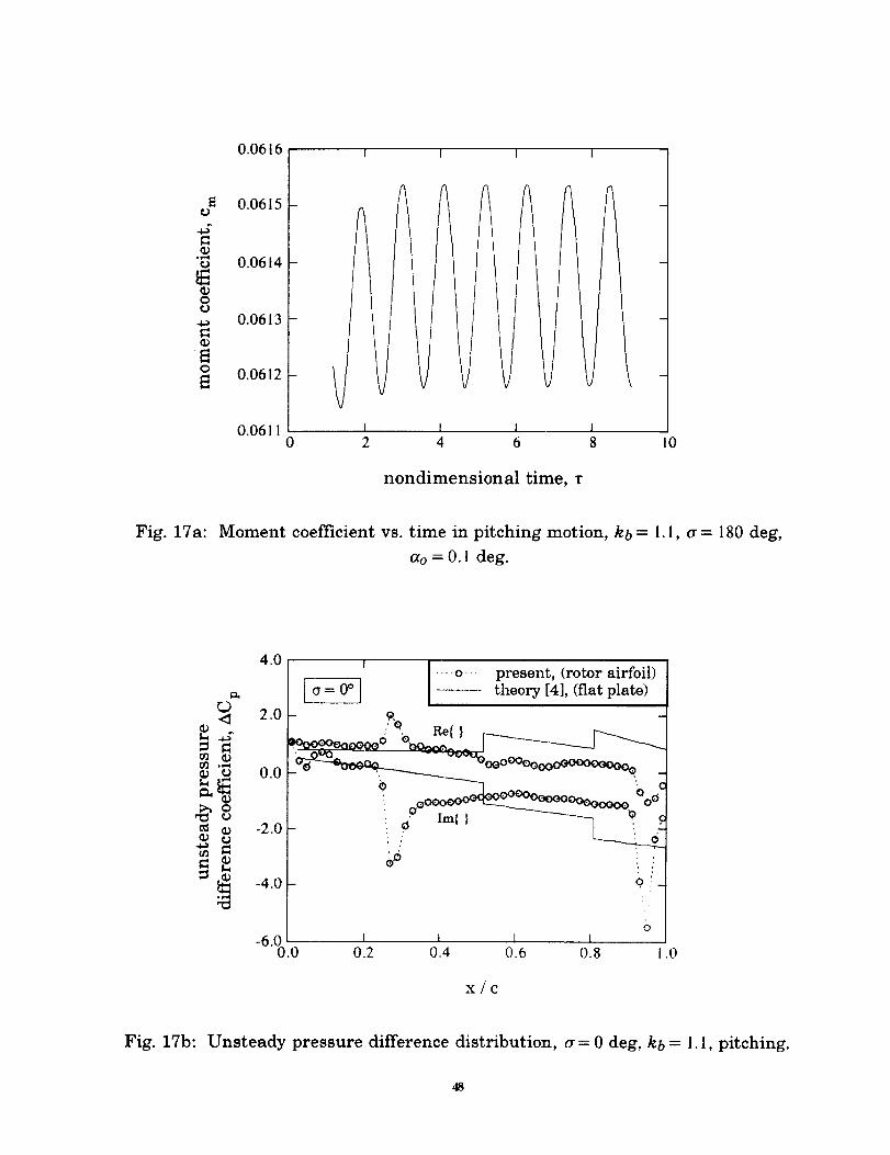
0.0616

0.0615

o_ 0.0614

0.0613

0

_ 0.06_2

0.0611 i

1 I II

I

I 1 I

0 2 4 6 8 10

nondimensional time, r

Fig. 17a: Moment coefficient vs. time in pitching motion, kb = 1.1, ¢r = 180 deg,

ao = 0.1 deg.

4.0

2.0

t..., ..,.¢I:::l

0'] . ,t,.-I

t,..,__ 0.0

t_ _ -2.0

._ -4.0

t J .... o present, (rotor airfoil)

i _ = t [ theory [4], (flat plate)o,:' Q. Re{}

-6.0 t I l t0.0 0.2 0.4 0.6 0.8

o.

O

x/c

.0

Fig. 17b: Unsteady pressure difference distribution, a= 0 deg, kb = l.l, pitching.

48

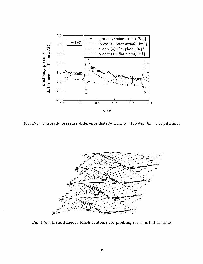
<1(D

¢J

{D c9

_D

q_

5.0 I [ .... o---

[r(x= 180°1] l present, (rotor airfoil), Re{}

4.0 .... +-- present, (rotor airfoil), Ira{ }

--- theory [4], (flat plate), Re{ }

3.0 - theory. [4], (flat plate), Im{ }

+ '

2.0 - _- ,:i -

0 OOo i':1.0 ]__°°ooooooooo, : :_ °°%ooOoo : ::-

-i .0/ O o

-2.0 [ [ I I I0.0 0.2 0.4 0.6 0.8 1.0

x/c

Fig. 17c: Unsteady pressure difference distribution, or= 180 deg, kb = l.l, pitching.

Fig. 17d: Instantaneous Mach contours for pitching rotor airfoil cascade

49

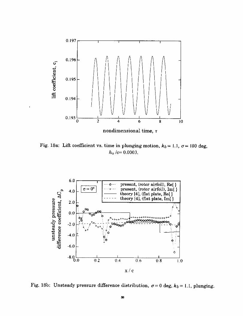
O. 197 I I I I

• _,-,i

0

0.196

0.195

0.194 -

I I I0.1930 2 4 6 8 10

nondimensional time, r

Fig. 18a: Lift coefficient vs. time in plunging motion, kb = 1.1, a= 180 deg,

ho /c= 0.0003.

6.0

4.0rD<1

_ -_ 2.0m _

_ 0.0

#° -2.0

_ -4.0

-6.0

-8.00.0

• ' [ .... o--- present, (rotor airfoil), Re{}

, - ..... ] +--- present, (rotor airfoil), Im{ }..... theory [4], (fiat plato, Re{ }

theory [4], (flat plato, Ira{ }

_a, ?_ _0 _. -q- _ + ++ _F +_e +.+ +-q..b+ + +_F .i._ .1_- _/_'' '

v_ " -_ "+'_-÷'_ +-_7 - - -

_,_ _._ . _:__,- _ _ _,¢_o.oy__-_-_____. _ Q-:- _ - -_ - ._- ? : .' _'_Oooo ......... I- - - _- -o"

',:o 6.4-

2 A t l

0.2 0.4 0.6 0.8 1.0

x/c

Fig. 18b: Unsteady pressure difference distribution, cr= 0 deg, kb = 1.1, plunging.

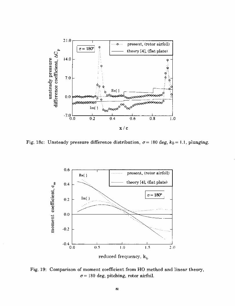
21.0 I

cr 180 ° o

.... 0''" present, (rotor airfoil)

theory [4], (flat plate)

x/c

Fig. 18c: Unsteady pressure difference distribution, _r= 180 deg, kb = 1.1, plunging.

0.6 r

0.4

. v.,._

o 0.2

0

._ 0.0

0

-0.2

-0.4 _--0.0 0.5

Re{ } .......... present, (rotor airfoil)

theory [4]__,(fla._ttplate.____)

1

I .0 I .5 2.0

reduced frequency, k b

Fig. 19: Comparison of moment coefficient from HO method and linear theory,

_r= 180 deg, pitching, rotor airfoil.

51

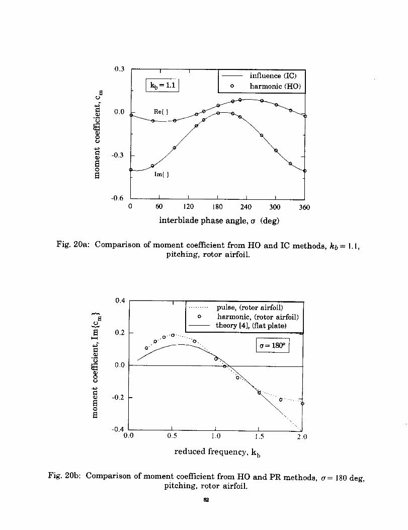
O

0.3

0.0

-0.3

-0.6

' ' I_ imquence (IC)

[ kb= 1.1 I ] o harmonic (HO)

hn{ }

I I I I I

60 120 180 240 300 360

interblade phase angle, o (deg)

Fig. 20a: Comparison of moment coefficient from HO and IC methods, kb = 1.1,

pitching, rotor airfoil.

_9

_=_

_J

O

09

O

0.4

0.2

0.0

-0.2 -

-0.40.0

......... pulse, (rotor airfoil)o harmonic, (rotor airfoil)

theory [4], (flat plate)

.o"-o ..... ..

° ° [ 1_ • a-- 180°

"0.,

\

"\

J- J I

0.5 ! .0 1.5 2.0

reduced frequency, k b

Fig. 20b: Comparison of moment coefficient from HO and PR methods, a = 180 deg,pitching, rotor airfoil.

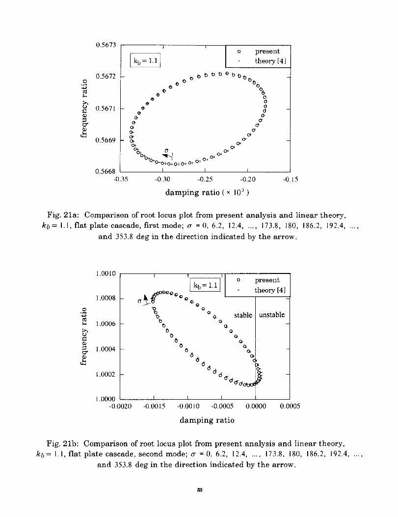
0.5673 , w

O

¢,9

0.5672

0.5671

0.5669

kb= 1.1

®- o

oo

o-<21--o-(3-

- o_-o+-o4-

o+. "_.-_0+0+0+ O+ 0+ 0+

I

-0.30

o present

÷ theory. [4]

0000

00-

O-0-

O-o_

o_-0_-

0.5668 l

-0.35 -0.25 -0.20 -0.15

damping ratio ( × 103 )

Fig. 21a: Comparison of root locus plot from present analysis and linear theory,

kb = I.l, flat plate cascade, firstmode; ¢r =0, 6.2, 12.4, ..., 173.8, 180, 186.2, 192.4, ...,

and 353.8 deg in the direction indicated by the arrow.

Oo_

¢9

1.0010

1.0008

1.0006

1.0004

1.0002

F 1"

\0

b0

Ikb--1.1JI©

QQ

Q0

00

66

0

o present

÷ theory [4]

stable

0

0-O-

QO-

unstable

1.0000

-0.0020 -0.0015 -O.OOlO -0.0005 0.0000 0.0005

damping ratio

Fig. 21b: Comparison of root locus plot from present analysis and linear theory,

kb = I.i, flat plate cascade, second mode; cr = 0. 6.2, 12.4, ..., 173.8, 180, 186.2, 192.4 .... ,

and 353.8 deg in the direction indicated by the arrow.

53

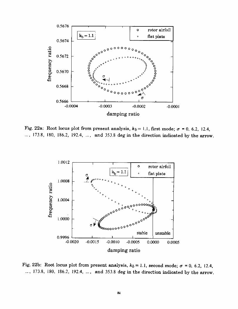
0.r-(

t_

c

0.5674 -

0.5672 -

0.5670 -

0.5668 -

0.5666-0.0004

o rotor airfoil

÷ flat plate

_000000_

0000v _0000

O0 ++4.+-t.++++++++ 0 0

0 + _4 0

o _+ +_ o0 _ .+ 0

o2+**+;÷÷+v. + ++*00 00

0 o 00

OooooooO_\0

, I , I ,

-0.0003 -0.0002

damping ratio

-0.0001

Fig. 22a: Root locus plot from present analysis, kb = 1. I, first mode; tr = 0, 6.2, 12.4,

.... 173.8, 180, 186.2, 192.4, ..., and 353.8 deg in the direction indicated by the arrow.

O

-4_

_9

1.00 !2 T T

1.0008

o rotor airfoil

+ flat plate

1.0004

1.0000

[kb= 1.1 l0

__ _-++++ + + + +4-

+4- + + +

+ ++ +

+ 4-+ +

4- +4- +

+ ++ 4-

+ + _,_o0000000_00"v+- "_

_000 '." + + + + 4-+._

O- _r"^0 0 0

O" _ _1:_00000"'_"J '_ 0 0 0 0 0 00000

stable.t l .t

-0.0015 -0.0010 -0.0005

unstable0.9996

-0.0020 0.0000 0.0005

damping ratio

Fig. 22b: Root locus plot from present analysis, kb = l.l, second mode; a = 0, 6.2, 12.4,

.... 173.8, 180, 186.2, 192.4 ..... and 353.8 deg in the direction indicated by the arrow.

64

Form Approved

REPORT DOCUMENTATION PAGE OMB No. 0704-0188

Public reporting burden lor this collection of information is estimated to average 1 hour per response, including the time for reviewing instructions, searching existing data sources,

gathering and maintaining the data needed, and completing and reviewing the collection ot information, Send comments regarding this burden estimate or any other aspect of this

collection of information, including suggestions for reducing this burden, to Washington Headquarters Services, Directo¢ate for information Operations and Reports, 1215 Jefferson

Davis Highway, Suite 1204, Arlington, VA 22202-4302, and to the Office of Management and Budget, Paperwork Reduction Project (0704-0188), Washington, DC 20503

1. AGENCY USE ONLY (Leave blank) I 2. REPORT DATE 3. REPORT TYPE AND DATES COVERED

August 1992

4. TITLE AND SUBTITLE

Flutter Analysis of Supersonic Axial Flow Cascades Using a High Resolution

Euler Solver

Part 1: Formulation and Validation

6. AUTHOR(S)

T.S.R. Reddy, Milind A. Bakhle, Dennis L. Huff, and Timothy W. Swafford

7. PERFORMING ORGANIZATION NAME(S) AND ADDRESS(ES)

National Aeronautics and Space Administration

Lewis Research Center

Cleveland, Ohio 44135-3191

9. SPONSORING/MONITORING AGENCY NAMES(S) AND ADDRESS(ES)

National Aeronautics and Space Administration

Washington, D.C. 20546-0001

Technical Mem_randum

5. FUNDING NUMBERS

WU-535-03-10

8. PERFORMING ORGANIZATIONREPORT NUMBER

E-7229

i0. SPONSORING/MONITORING

AGENCY REPORT NUMBER

NASA TM- 105798

11. SUPPLEMENTARY NOTES

T.S.R. Reddy and M.A. Bakhle, University of Toledo, Department of Mechanical Engineering, Toledo, Ohio 436t1(', and NASA Resident Research

Associate at Lewis Research Center. D.L. Ituff, NASA Lewis Research Ccnlcr, Clcvchmd. Ohi(_. T.W. Swaft'_rd, Mississippi State University,

Dcpartmenl of Aerospace Engineering, Mississippi State, Mississippi 39762. Responsible person, Gc(_rgc L. Stc['ko, (216)433-3921).

1'2 "2b. DISTRIBUTION CODE

Date for general re|case

Subject Category 39

August 19'-;'4

13. ABSTRACT(Maximum 200 words)

This report presents, in two parts, a dynamic aeroelastie stability (flutter) analysis of a cascade of blades in supersonic axial flow. Each

blade of the cascade is modeled as a typical section having pitching and plunging degrees of freedom. Aerodynamic forces are obtained

from a time accurate, unsteady, two-dimensional cascade solver based on the Euler equations. The solver uses a time marching flux-

difference splitting (FDS) scheme. Flutter stability is analyzed in the frequency domain. The unsteady force coefficients required in the

analysis are obtained by harmonically oscillating (HO) the blades for a given flow condition, oscillation frequency, and interblade phase

angle. The calculated time history of the forces is then Fourier decomposed to give the required unsteady fi)rce coefficients. An

influence coefficient tIC) method and a pulse response (PR) method are also implemented to reduce the computational time for the

calculation of the unsteady force coefficients for any phase angle and oscillation frequency. Part I, this report, presents these analysis

methods, and their validation by comparison with results obtained from linear theory for a selected flat plate cascade geometry. A

typical calculation for a rotor airfoil is also included to show the applicability of the present solver for airfoil configurations. The

predicted unsteady aerodynamic forces for a selected flat plate cascade geometry, and flow conditions correlated well with those

obtained from linear theory for different interblade phase angles and oscillation frequencies. All the three methods of predicting

unsteady force coefficients, namely, HO, IC and PR showed good correlation with each other. It was established that only a single

calculation with four blade passages is required to calculate the aerodynamic forces for any phase angle for a cascade consisting of any

number of blades, for any value of the oscillation frequency. Flutter results, including mistuning effects, fi)r a cascade of stator airfoils

arc presented in Part 2 of the report.

14. SUBJECT TERMS

Cascades; Supersonic axial flow; Flutter; Euler; Harmonic oscillation; Influence coeffi-

cient; Pulse response; Frequency domain

17. SECURITy CLASSIFICATION 18. SECURITY CLASSIFICATION'

OF REPORT OF THIS PAGE

Unclassified Unclassified

NSN 7540-01-280-5500

119. SECURITY CLASSIFICATION

OF ABSTRACT

Unclassified

15. NUMBER OF PAGES

5616. PRICE CODE

A0420. LIMITATION OF ABSTRACT

Standard Form 298 trey. 2-89)Prescribed by ANSI Std. Z39-18298-102