Embed Size (px)
Citation preview
EURUS MINERAL CONSULTANTS: User Manual for KinCalc™ v3.1 , June 2008 Page 1 of 118
Eurus Mineral Consultants © 2002-2008. Copyright subsists in this work.
Flotation Kinetics Calculator
Incorporating
KinCalc® ScrollCalc® Tabulation of data Graphing facility Statistical functions Access or SQL Database
USER MANUAL
eurus mineral consultants
EURUS MINERAL CONSULTANTS: User Manual for KinCalc™ v3.1 , June 2008 Page 2 of 118
Eurus Mineral Consultants © 2002-2008. Copyright subsists in this work.
CONTENTS
1. COPYRIGHT AND DISCLAIMER ............................................................................................ 6
2. SYSTEM REQUIREMENTS AND INSTALLING KINCALC™ .......................................... 7
2.1. INTRODUCTION .......................................................................................................................... 7
2.2. PRE-REQUISITES .......................................................................................................................... 7
2.3. INSTALLATION ............................................................................................................................ 8
2.4. DOCUMENTATION ..................................................................................................................... 8
2.5. THE HASP DRIVERS ................................................................................................................... 8
2.6. THE KINCALC™ SPREADSHEET ............................................................................................ 9
2.7. THE KINCALC™ DATABASE ................................................................................................... 9
2.7.1. SHARED DATABASE ON A NETWORK ........................................................................ 9
2.7.2. STANDALONE DATABASE ............................................................................................. 12
2.8. THE EMC™ EXCEL UTILITIES ................................................................................................ 12
2.9. FIRST-TIME USE ......................................................................................................................... 12
2.9.1. KINCALC™ DATABASE ................................................................................................... 12
2.9.2. KINCALC™ SPREADSHEET ............................................................................................ 15
2.9.3. LOCATE THE KINCALC™ DATABASE ........................................................................ 16
2.10. UNINSTALLATION .................................................................................................................. 19
3. IMPORTANT POINTS REGARDING INITIAL SET-UP AND USE OF THE KINCALC™ KINETICS CALCULATOR .................................................................................. 20
4. INTRODUCTION TO THE FLOTATION KINETICS CALCULATOR ........................... 25
4.1. WHAT ARE FLOTATION KINETICS? ................................................................................... 25
4.2. TERMINOLOGY AND ACRONYMS ...................................................................................... 27
4.3. BRIEF OVERVIEW OF THE KINETICS CALCULATOR .......................................................... 27
5. TOOLBAR ICONS ....................................................................................................................... 32
5.1. STANDARD ICONS .............................................................................................................. 32
5.2. OPTIONAL EXTRA ICONS ................................................................................................... 33
6. DEFINING ANALYTES, MINERALS AND FLOATABLE GANGUE .............................. 35
6.1. MANAGING ANALYTES AND MINERALS .......................................................................... 35
6.2. ORDERING ANALYTES AND SAVING ANALYTE SETS ...................................................... 35
6.3. ANALYTE ALIASES .............................................................................................................. 35
6.4. SETTING YOUR OWN SYMBOL OR ACRONYM FOR A STANDARD ASSAY UNIT ............ 36
6.5. CHANGING ASSAY UNITS FOR THE KINCALC™ PROGRAM .......................................... 36
6.6. CHANGING ASSAY UNITS AND DECIMAL PLACES ON THE INPUT PAGE ....................... 37
6.7. DETERMINING THE CATEGORY OF AN ANALYTE ............................................................. 39
EURUS MINERAL CONSULTANTS: User Manual for KinCalc™ v3.1 , June 2008 Page 3 of 118
Eurus Mineral Consultants © 2002-2008. Copyright subsists in this work.
7. DEFINING STREAM NAMES .................................................................................................. 42
8. DEFINING OTHER TEST PARAMETERS ............................................................................ 43
8.1. MANAGING OTHER TEST PARAMETERS .......................................................................... 43
8.2. INSERTING A COLUMN AT A LATER STAGE AFTER FLOTATION KINETICS HAVE BEEN
CALCULATED ................................................................................................................ 45
9. MANUAL INPUT OF TEST DATA .......................................................................................... 47
9.1. MANUAL INPUT OF TEST DATA ........................................................................................ 47
9.2. MANUAL INPUT OF OTHER TEST PARAMETERS .............................................................. 47
10. AUTOMATED IMPORTING OF TEST DATA ..................................................................... 49
10.1. SPECIFYING IF ASSAY DATA IS FORMATTED AS A “SINGLE REGION” .................... 49
10.2. IMPORT WIZARD ......................................................................................................... 50
10.3. MAKING A NEW IMPORT FORMAT – ONE DATA SET PER SHEET ........................... 50
10.4. MAKING A NEW IMPORT FORMAT – MULTIPLE DATA SETS PER SHEET ................ 53
10.5. MAKING A NEW IMPORT FORMAT – FROM A KINCALC™ DATA SHEET ............... 54
10.6. DEFINING AND SETTING-UP OTHER PARAMETERS ................................................. 55
10.7. IMPORTING DATA – SINGLE MODE .......................................................................... 55
10.8. IMPORTING DATA – BATCH MODE ........................................................................... 58
11. CALCULATING KINETICS ...................................................................................................... 60
11.1. AUTOMATIC CALCULATION OF KINETICS ................................................................ 60
11.2. MANUAL CALCULATION OF KINETICS VIA THE INPUT PAGE .................................. 60
11.3. MANUAL CALCULATION OF KINETICS VIA SCROLLCALC™ ................................... 61
12. RESULTS SHEET ......................................................................................................................... 62
12.1 BOUNDARY TEST SETTINGS .............................................................................................. 62
13. SUMMARY SHEET ..................................................................................................................... 65
13.1. FUNCTIONS AVAILABLE TO PROCESS AND ARRANGE DATA .................................. 66
13.2. MISC PARAMETERS ..................................................................................................... 70
13.3. KELSALL PARAMETERS, AFTER BOUNDARY TESTS AND AFTER SCROLLCALC™ .. 71
13.4. LINEAR CORRELATION COEFFICIENTS ...................................................................... 71
13.5. SUM OF SQUARED ERRORS (BASED ON BOUNDARY TEST PARAMETERS) .............. 71
13.6. SLOW FLOATING RATIO ............................................................................................. 71
13.7. SELECTIVITY ................................................................................................................ 72
13.8. MEASURED RECOVERIES AND CONCENTRATE GRADES .......................................... 72
EURUS MINERAL CONSULTANTS: User Manual for KinCalc™ v3.1 , June 2008 Page 4 of 118
Eurus Mineral Consultants © 2002-2008. Copyright subsists in this work.
13.9. CALCULATED HEAD GRADES ..................................................................................... 72
13.10. FLOATABILITY .............................................................................................................. 72
14. DATA SHEET ............................................................................................................................... 72
15. AVERAGE SHEET ....................................................................................................................... 73
16. SCROLLCALC™ .......................................................................................................................... 74
16.1. LOADING DATA INTO SCROLLCALC™ ...................................................................... 74
16.2. USING THE SCROLLCALC™ PAGE ............................................................................. 75
16.3. CLEARING AND TRANSFERRING DATA TO THE SUMMARY SHEET ......................... 76
16.4. IDENTIFYING SUSPECT KINETIC VALUES .................................................................. 77
16.5. METHOD FOR DETERMINING KINETIC VALUES MANUALLY .................................. 78
16.6. GUIDELINES FOR KINETIC VALUES ............................................................................ 83
17. ACCESS OR SQL DATABASE ................................................................................................. 89
17.1. POSTING DATA TO THE ACCESS OR SQL DATABASE .............................................. 89
17.2. IMPORTING DATA FROM THE ACCESS OR SQL DATABASE INTO THE SUMMARY
SHEET ........................................................................................................................... 89
18. GRAPHING FACILITY .............................................................................................................. 91
18.1. USING THE CUSTOM GRAPHS .................................................................................... 91
19. CUSTOMISING THE GRAPHING FACILITY & PROGRAM SETTINGS .................... 92
19.1. GRAPH SETTINGS ........................................................................................................ 92
19.2. GRAPH SERIES ............................................................................................................. 94
19.3. FILE LOCATIONS .......................................................................................................... 94
19.4. USER INTERFACE ......................................................................................................... 94
20. EMC™ EXCEL UTILITIES ......................................................................................................... 97
20.1. THE TOOLBAR.............................................................................................................. 97
20.2. THE TRANSPOSE FUNCTIONS ..................................................................................... 99
20.3. THE CORRELATION MATRIX FUNCTION ................................................................. 105
20.4. THE FREQUENCY PLOT FUNCTION ........................................................................... 111
20.5. CHANGE DEFAULT SETTINGS FOR EMC™ TOOLS ................................................ 113
21. MEANING AND USE OF FLOTATION KINETICS .......................................................... 116
21.1. USES OF THE FLOTATION KINETICS CALCULATOR ................................................ 116
21.2. A CASE STUDY IN WHAT FLOTATION KINETICS MEAN .......................................... 116
EURUS MINERAL CONSULTANTS: User Manual for KinCalc™ v3.1 , June 2008 Page 5 of 118
Eurus Mineral Consultants © 2002-2008. Copyright subsists in this work.
LIST OF TABLES
Table 1 Simulated vs. Actual Mass Balances 118 Table 2 Flotation Kinetic Changes 118
LIST OF FIGURES
Figure 1 One-Glance Layout of Program Functions in “Mind Map” Format ............................... 29 Figure 2 Flow Diagram of KinCalc’s™ Main Functions ................................................................... 30 Figure 3 Simplified Outline of KinCalc’s™ Main Functions ............................................................ 31 Figure 4 Full Screen of Input Page showing Icons ............................................................................ 34 Figure 5 Flotation Circuit before Optimisation ................................................................................ 117 Figure 6 Flotation Circuit after Optimisation ................................................................................... 118

EURUS MINERAL CONSULTANTS: User Manual for KinCalc™ v3.1 , June 2008 Page 6 of 118
Eurus Mineral Consultants © 2002-2008. Copyright subsists in this work.
1. COPYRIGHT AND DISCLAIMER
Disclaimer This work was created with due application of professional and intellectual skills, knowledge and
expertise. EURUS MINERAL CONSULTANTS CC however takes no responsibility for any loss
occasioned by the use of the information contained in this work.
Copyright
© 2007. Copyright subsists in this work. No part of this work may be reproduced or copied in any way
without the written consent from EURUS MINERAL CONSULTANTS CC. Any unauthorised
reproduction of this work will constitute copyright infringement and render the doer liable under criminal
and civil law.
All rights reserved.
EURUS MINERAL CONSULTANTS: User Manual for KinCalc™ v3.1 , June 2008 Page 7 of 118
Eurus Mineral Consultants © 2002-2008. Copyright subsists in this work.
2. SYSTEM REQUIREMENTS AND INSTALLING KINCALC®
Contents:
1. Installation: Standalone and Network 2. HASP security drivers 3. KinCalc® database 4. EMC Excel utilities 5. First-Time Use: KinCalc® spreadsheet, Confirm solver reference 6. Uninstall
Diagrams highlighting various points detailed below can be found towards the end of this section.
2.1. Introduction
The KinCalc® system consists of several components: The KinCalc® Spreadsheet
The KinCalc® Database
The EMC Excel Utilities
The Aladdin HASP Software Protection System
Supporting documentation including the user manual
This document provides instructions to guide a user through the steps required to install the above components.
2.2. Pre-Requisites
The KinCalc® suite was written using the Microsoft Office 2002® programs of MS Excel® and MS Access® and SQL. Although standard MS Office components were used, the KinCalc® suite is not guaranteed to work with earlier versions of MS Office. Before installing and using KinCalc®, the end-user computer should meet the following requirements:
MS Office 2002 Professional must be installed;
The Solver® component of MS Excel must be installed;
The user must have administrative privileges on the computer where the KinCalc® component is being installed;
There must be approximately 12 Mb of free space on the destination drive.
Acrobat Reader® version 5 or greater is required to read the installation and user manual documents.
EURUS MINERAL CONSULTANTS: User Manual for KinCalc™ v3.1 , June 2008 Page 8 of 118
Eurus Mineral Consultants © 2002-2008. Copyright subsists in this work.
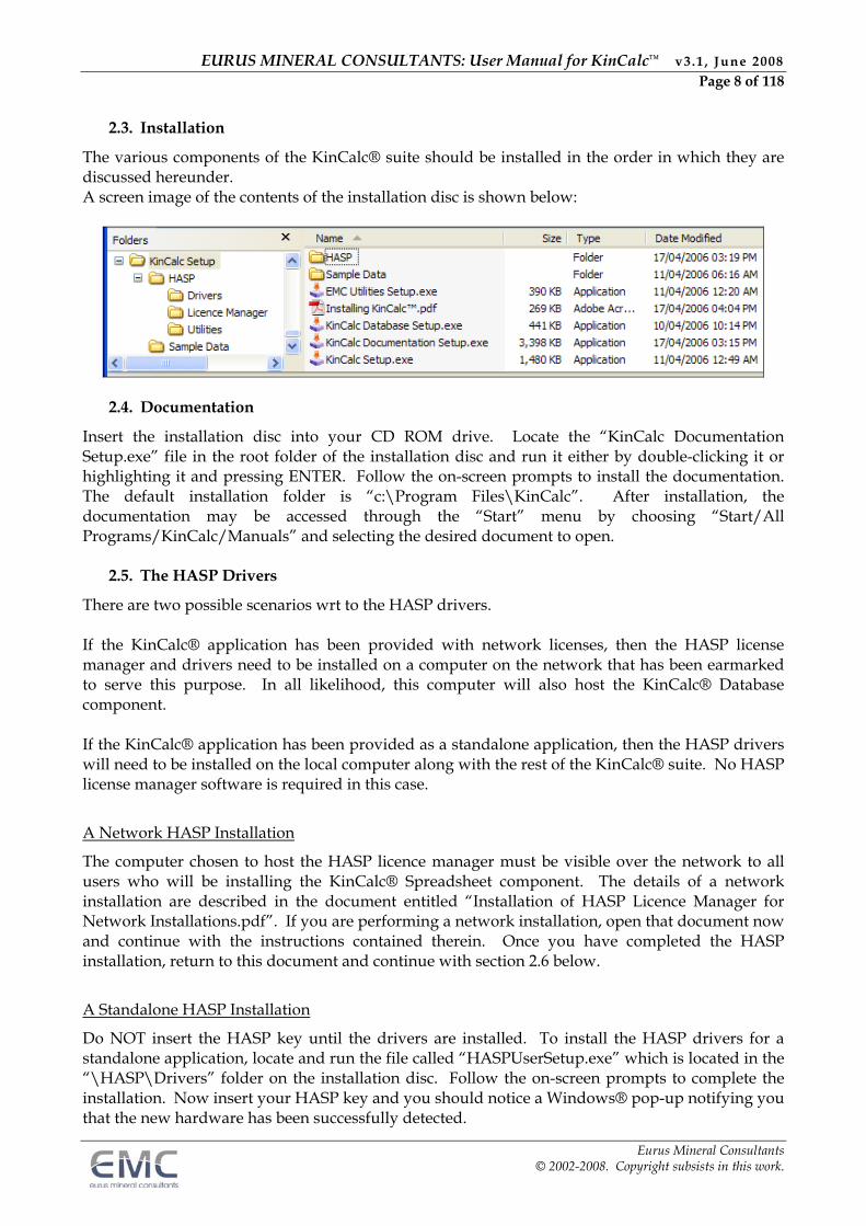
2.3. Installation
The various components of the KinCalc® suite should be installed in the order in which they are discussed hereunder. A screen image of the contents of the installation disc is shown below:
2.4. Documentation
Insert the installation disc into your CD ROM drive. Locate the “KinCalc Documentation Setup.exe” file in the root folder of the installation disc and run it either by double-clicking it or highlighting it and pressing ENTER. Follow the on-screen prompts to install the documentation. The default installation folder is “c:\Program Files\KinCalc”. After installation, the documentation may be accessed through the “Start” menu by choosing “Start/All Programs/KinCalc/Manuals” and selecting the desired document to open.
2.5. The HASP Drivers
There are two possible scenarios wrt to the HASP drivers. If the KinCalc® application has been provided with network licenses, then the HASP license manager and drivers need to be installed on a computer on the network that has been earmarked to serve this purpose. In all likelihood, this computer will also host the KinCalc® Database component. If the KinCalc® application has been provided as a standalone application, then the HASP drivers will need to be installed on the local computer along with the rest of the KinCalc® suite. No HASP license manager software is required in this case.
A Network HASP Installation
The computer chosen to host the HASP licence manager must be visible over the network to all users who will be installing the KinCalc® Spreadsheet component. The details of a network installation are described in the document entitled “Installation of HASP Licence Manager for Network Installations.pdf”. If you are performing a network installation, open that document now and continue with the instructions contained therein. Once you have completed the HASP installation, return to this document and continue with section 2.6 below.
A Standalone HASP Installation
Do NOT insert the HASP key until the drivers are installed. To install the HASP drivers for a standalone application, locate and run the file called “HASPUserSetup.exe” which is located in the “\HASP\Drivers” folder on the installation disc. Follow the on-screen prompts to complete the installation. Now insert your HASP key and you should notice a Windows® pop-up notifying you that the new hardware has been successfully detected.
EURUS MINERAL CONSULTANTS: User Manual for KinCalc™ v3.1 , June 2008 Page 9 of 118
Eurus Mineral Consultants © 2002-2008. Copyright subsists in this work.
2.6. The KinCalc® Spreadsheet
The KinCalc® Spreadsheet component may not be installed as a shared network component. Each user that is to use the KinCalc® Spreadsheet should install the appropriate files on their own computer on their local hard disk. The KinCalc® Spreadsheet application may not simply be copied from one computer to another as it will not function. To install the spreadsheet component, locate and run the file entitled “KinCalc Setup.exe” which is stored in the root folder of the installation disc. Follow the on-screen prompts to accept the licence agreement and install the spreadsheet component of KinCalc®. The default installation folder is “c:\Program Files\KinCalc”. The KinCalc® Spreadsheet may be accessed either from the newly created desktop shortcut or through the “Start” menu by choosing “Start/All Programs/KinCalc/KinCalc”.
2.7. The KinCalc® Database
Only one instance of the KinCalc® Database component should be installed. If the KinCalc® license agreement is a network based agreement, then install the database component on a shared folder on a network computer. As already suggested, it is likely to be the same computer where the HASP license manager was installed. Continue with the instructions in the section “Shared Database on a Network” below.
If the licence agreement is for a standalone version, then install the database component on the local computer. Continue with the instructions in section “Standalone Database” below.
2.7.1. Shared Database on a Network
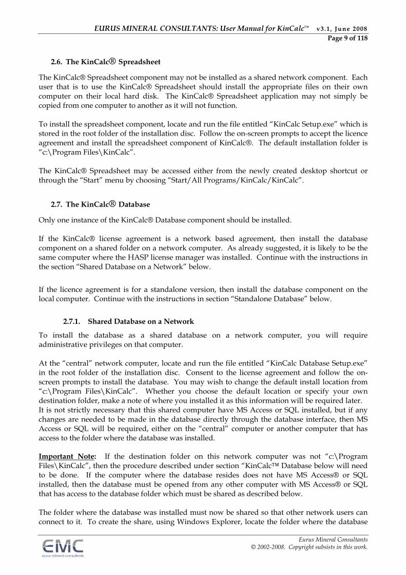
To install the database as a shared database on a network computer, you will require administrative privileges on that computer. At the “central” network computer, locate and run the file entitled “KinCalc Database Setup.exe” in the root folder of the installation disc. Consent to the license agreement and follow the on-screen prompts to install the database. You may wish to change the default install location from “c:\Program Files\KinCalc”. Whether you choose the default location or specify your own destination folder, make a note of where you installed it as this information will be required later. It is not strictly necessary that this shared computer have MS Access or SQL installed, but if any changes are needed to be made in the database directly through the database interface, then MS Access or SQL will be required, either on the “central” computer or another computer that has access to the folder where the database was installed. Important Note: If the destination folder on this network computer was not “c:\Program Files\KinCalc”, then the procedure described under section “KinCalc™ Database below will need to be done. If the computer where the database resides does not have MS Access® or SQL installed, then the database must be opened from any other computer with MS Access® or SQL that has access to the database folder which must be shared as described below. The folder where the database was installed must now be shared so that other network users can connect to it. To create the share, using Windows Explorer, locate the folder where the database
EURUS MINERAL CONSULTANTS: User Manual for KinCalc™ v3.1 , June 2008 Page 10 of 118
Eurus Mineral Consultants © 2002-2008. Copyright subsists in this work.
was installed. In the example below, the default install folder was used, so the database files reside in “c:\Program Files\KinCalc”. The following screen images and procedures may depend on the operating system installed on the “central” computer. The procedure may differ on a computer with Windows Server 2003. The example below was generated under Windows XP. Locate the database install folder and then right-click it and choose “Sharing and Security. . .” . . .
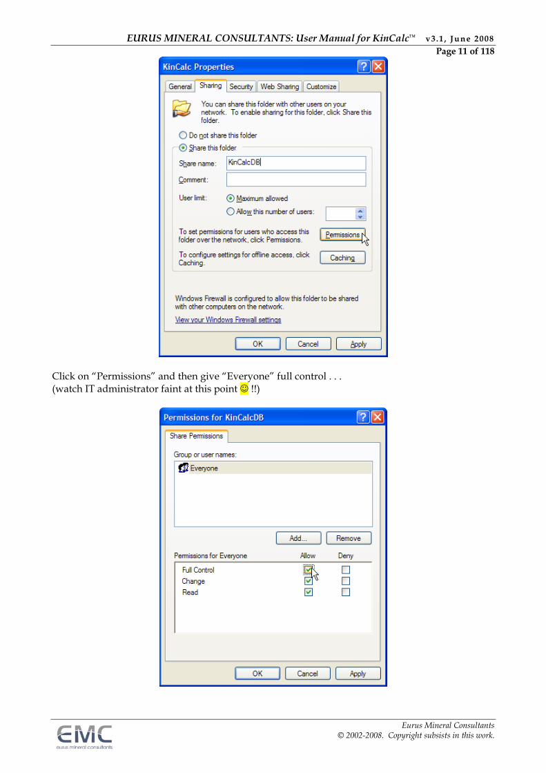
Click on the “Share this folder” option and enter a share name that is easy to remember, e.g. “KinCalcDB” . . .
EURUS MINERAL CONSULTANTS: User Manual for KinCalc™ v3.1 , June 2008 Page 11 of 118
Eurus Mineral Consultants © 2002-2008. Copyright subsists in this work.
Click on “Permissions” and then give “Everyone” full control . . . (watch IT administrator faint at this point !!)
EURUS MINERAL CONSULTANTS: User Manual for KinCalc™ v3.1 , June 2008 Page 12 of 118
Eurus Mineral Consultants © 2002-2008. Copyright subsists in this work.
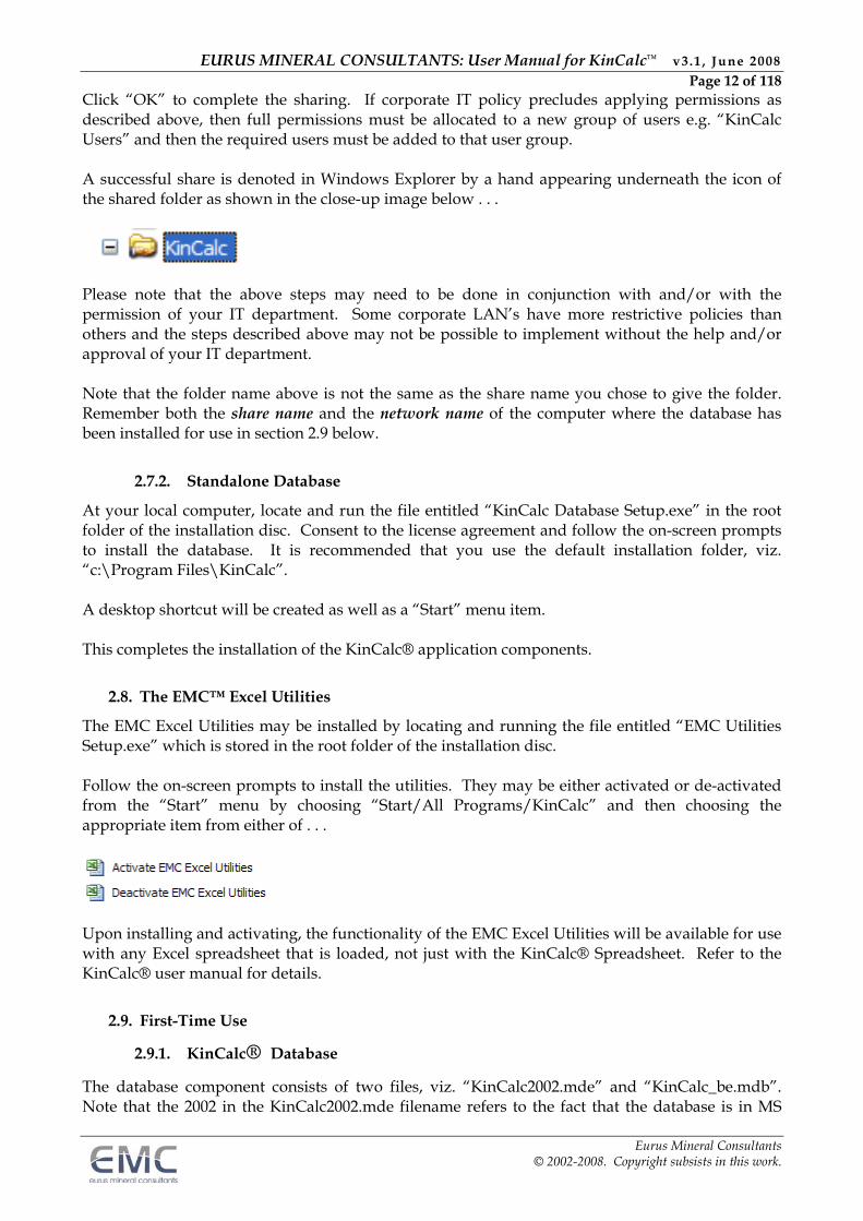
Click “OK” to complete the sharing. If corporate IT policy precludes applying permissions as described above, then full permissions must be allocated to a new group of users e.g. “KinCalc Users” and then the required users must be added to that user group. A successful share is denoted in Windows Explorer by a hand appearing underneath the icon of the shared folder as shown in the close-up image below . . .
Please note that the above steps may need to be done in conjunction with and/or with the permission of your IT department. Some corporate LAN’s have more restrictive policies than others and the steps described above may not be possible to implement without the help and/or approval of your IT department. Note that the folder name above is not the same as the share name you chose to give the folder. Remember both the share name and the network name of the computer where the database has been installed for use in section 2.9 below.
2.7.2. Standalone Database
At your local computer, locate and run the file entitled “KinCalc Database Setup.exe” in the root folder of the installation disc. Consent to the license agreement and follow the on-screen prompts to install the database. It is recommended that you use the default installation folder, viz. “c:\Program Files\KinCalc”. A desktop shortcut will be created as well as a “Start” menu item. This completes the installation of the KinCalc® application components.
2.8. The EMC™ Excel Utilities
The EMC Excel Utilities may be installed by locating and running the file entitled “EMC Utilities Setup.exe” which is stored in the root folder of the installation disc. Follow the on-screen prompts to install the utilities. They may be either activated or de-activated from the “Start” menu by choosing “Start/All Programs/KinCalc” and then choosing the appropriate item from either of . . .
Upon installing and activating, the functionality of the EMC Excel Utilities will be available for use with any Excel spreadsheet that is loaded, not just with the KinCalc® Spreadsheet. Refer to the KinCalc® user manual for details.
2.9. First-Time Use
2.9.1. KinCalc® Database
The database component consists of two files, viz. “KinCalc2002.mde” and “KinCalc_be.mdb”. Note that the 2002 in the KinCalc2002.mde filename refers to the fact that the database is in MS
EURUS MINERAL CONSULTANTS: User Manual for KinCalc™ v3.1 , June 2008 Page 13 of 118
Eurus Mineral Consultants © 2002-2008. Copyright subsists in this work.
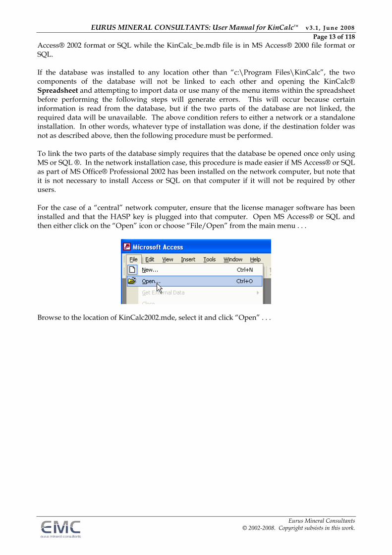
Access® 2002 format or SQL while the KinCalc_be.mdb file is in MS Access® 2000 file format or SQL. If the database was installed to any location other than “c:\Program Files\KinCalc”, the two components of the database will not be linked to each other and opening the KinCalc® Spreadsheet and attempting to import data or use many of the menu items within the spreadsheet before performing the following steps will generate errors. This will occur because certain information is read from the database, but if the two parts of the database are not linked, the required data will be unavailable. The above condition refers to either a network or a standalone installation. In other words, whatever type of installation was done, if the destination folder was not as described above, then the following procedure must be performed. To link the two parts of the database simply requires that the database be opened once only using MS or SQL ®. In the network installation case, this procedure is made easier if MS Access® or SQL as part of MS Office® Professional 2002 has been installed on the network computer, but note that it is not necessary to install Access or SQL on that computer if it will not be required by other users. For the case of a “central” network computer, ensure that the license manager software has been installed and that the HASP key is plugged into that computer. Open MS Access® or SQL and then either click on the “Open” icon or choose “File/Open” from the main menu . . .
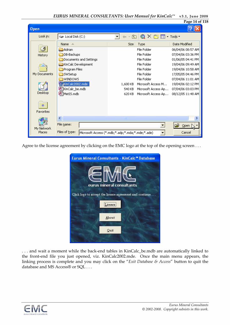
Browse to the location of KinCalc2002.mde, select it and click “Open” . . .
EURUS MINERAL CONSULTANTS: User Manual for KinCalc™ v3.1 , June 2008 Page 14 of 118
Eurus Mineral Consultants © 2002-2008. Copyright subsists in this work.
Agree to the license agreement by clicking on the EMC logo at the top of the opening screen . . .
. . . and wait a moment while the back-end tables in KinCalc_be.mdb are automatically linked to the front-end file you just opened, viz. KinCalc2002.mde. Once the main menu appears, the linking process is complete and you may click on the “Exit Database & Access” button to quit the database and MS Access® or SQL . . .
EURUS MINERAL CONSULTANTS: User Manual for KinCalc™ v3.1 , June 2008 Page 15 of 118
Eurus Mineral Consultants © 2002-2008. Copyright subsists in this work.
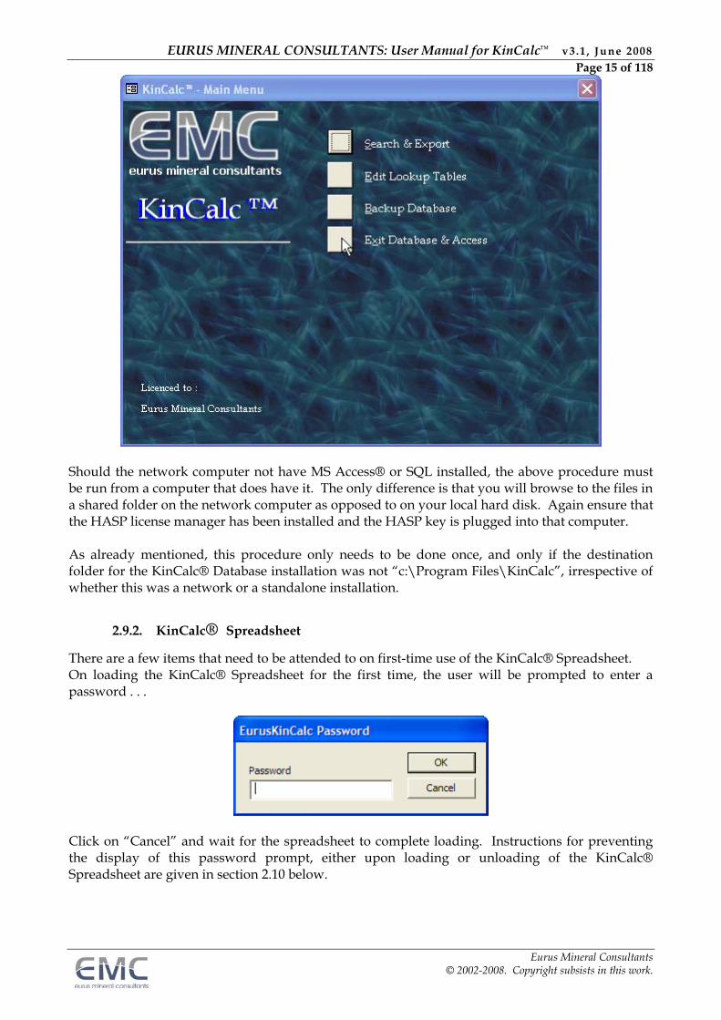
Should the network computer not have MS Access® or SQL installed, the above procedure must be run from a computer that does have it. The only difference is that you will browse to the files in a shared folder on the network computer as opposed to on your local hard disk. Again ensure that the HASP license manager has been installed and the HASP key is plugged into that computer. As already mentioned, this procedure only needs to be done once, and only if the destination folder for the KinCalc® Database installation was not “c:\Program Files\KinCalc”, irrespective of whether this was a network or a standalone installation.
2.9.2. KinCalc® Spreadsheet
There are a few items that need to be attended to on first-time use of the KinCalc® Spreadsheet. On loading the KinCalc® Spreadsheet for the first time, the user will be prompted to enter a password . . .
Click on “Cancel” and wait for the spreadsheet to complete loading. Instructions for preventing the display of this password prompt, either upon loading or unloading of the KinCalc® Spreadsheet are given in section 2.10 below.
EURUS MINERAL CONSULTANTS: User Manual for KinCalc™ v3.1 , June 2008 Page 16 of 118
Eurus Mineral Consultants © 2002-2008. Copyright subsists in this work.
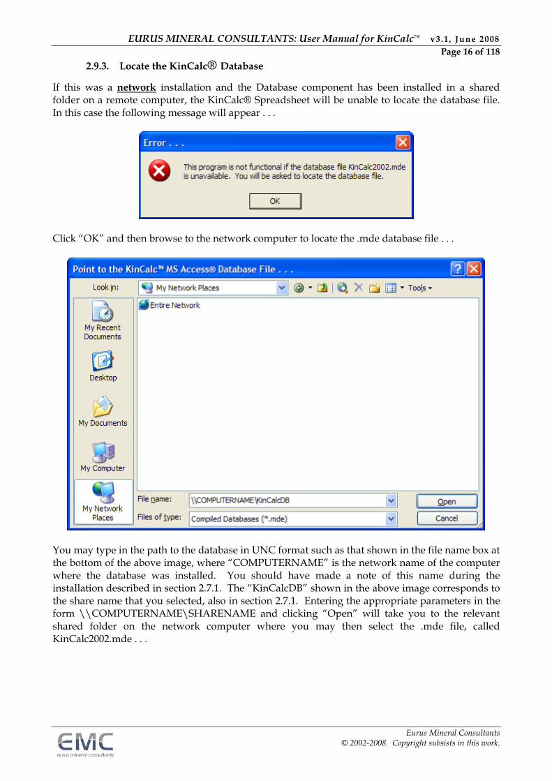
2.9.3. Locate the KinCalc® Database
If this was a network installation and the Database component has been installed in a shared folder on a remote computer, the KinCalc® Spreadsheet will be unable to locate the database file. In this case the following message will appear . . .
Click “OK” and then browse to the network computer to locate the .mde database file . . .
You may type in the path to the database in UNC format such as that shown in the file name box at the bottom of the above image, where “COMPUTERNAME” is the network name of the computer where the database was installed. You should have made a note of this name during the installation described in section 2.7.1. The “KinCalcDB” shown in the above image corresponds to the share name that you selected, also in section 2.7.1. Entering the appropriate parameters in the form \\COMPUTERNAME\SHARENAME and clicking “Open” will take you to the relevant shared folder on the network computer where you may then select the .mde file, called KinCalc2002.mde . . .
EURUS MINERAL CONSULTANTS: User Manual for KinCalc™ v3.1 , June 2008 Page 17 of 118
Eurus Mineral Consultants © 2002-2008. Copyright subsists in this work.
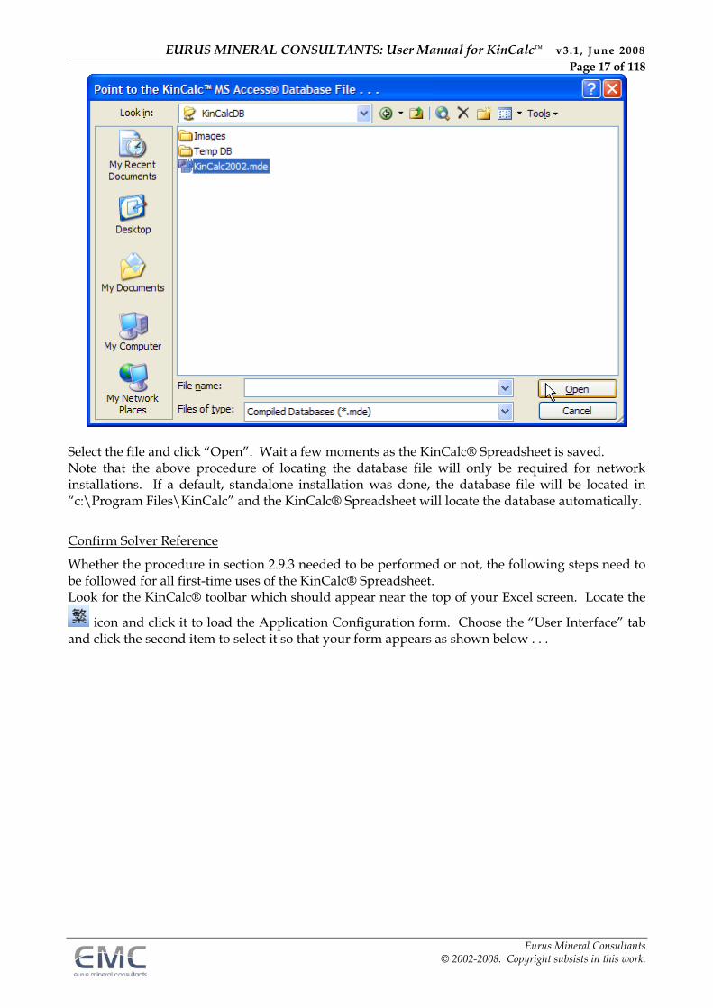
Select the file and click “Open”. Wait a few moments as the KinCalc® Spreadsheet is saved. Note that the above procedure of locating the database file will only be required for network installations. If a default, standalone installation was done, the database file will be located in “c:\Program Files\KinCalc” and the KinCalc® Spreadsheet will locate the database automatically.
Confirm Solver Reference
Whether the procedure in section 2.9.3 needed to be performed or not, the following steps need to be followed for all first-time uses of the KinCalc® Spreadsheet. Look for the KinCalc® toolbar which should appear near the top of your Excel screen. Locate the
icon and click it to load the Application Configuration form. Choose the “User Interface” tab and click the second item to select it so that your form appears as shown below . . .
EURUS MINERAL CONSULTANTS: User Manual for KinCalc™ v3.1 , June 2008 Page 18 of 118
Eurus Mineral Consultants © 2002-2008. Copyright subsists in this work.
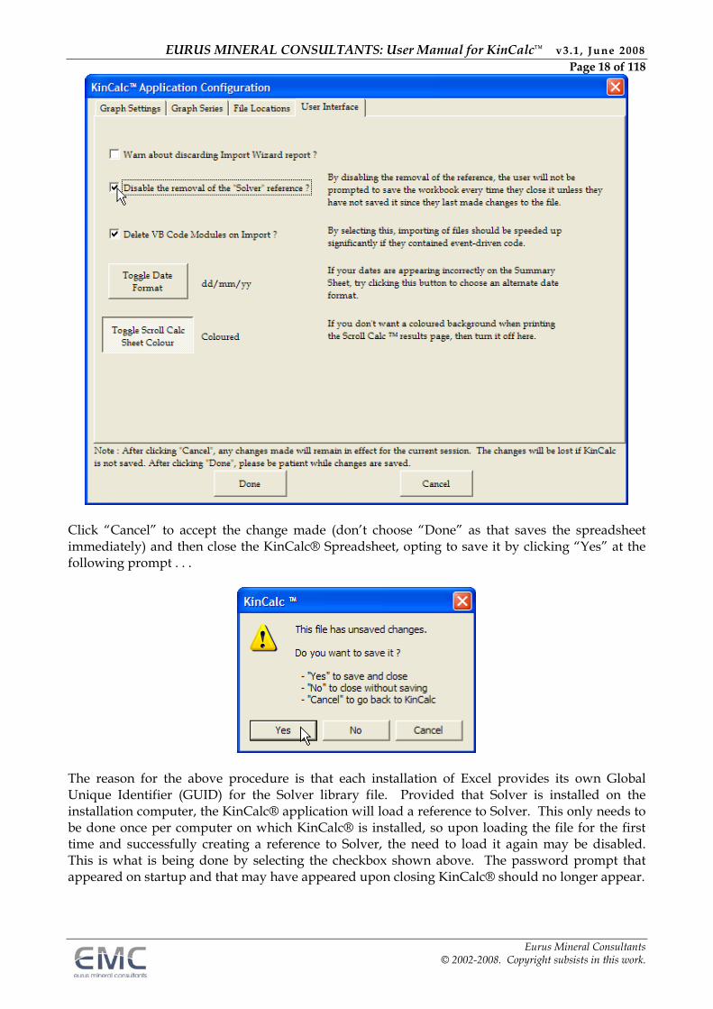
Click “Cancel” to accept the change made (don’t choose “Done” as that saves the spreadsheet immediately) and then close the KinCalc® Spreadsheet, opting to save it by clicking “Yes” at the following prompt . . .
The reason for the above procedure is that each installation of Excel provides its own Global Unique Identifier (GUID) for the Solver library file. Provided that Solver is installed on the installation computer, the KinCalc® application will load a reference to Solver. This only needs to be done once per computer on which KinCalc® is installed, so upon loading the file for the first time and successfully creating a reference to Solver, the need to load it again may be disabled. This is what is being done by selecting the checkbox shown above. The password prompt that appeared on startup and that may have appeared upon closing KinCalc® should no longer appear.
EURUS MINERAL CONSULTANTS: User Manual for KinCalc™ v3.1 , June 2008 Page 19 of 118
Eurus Mineral Consultants © 2002-2008. Copyright subsists in this work.
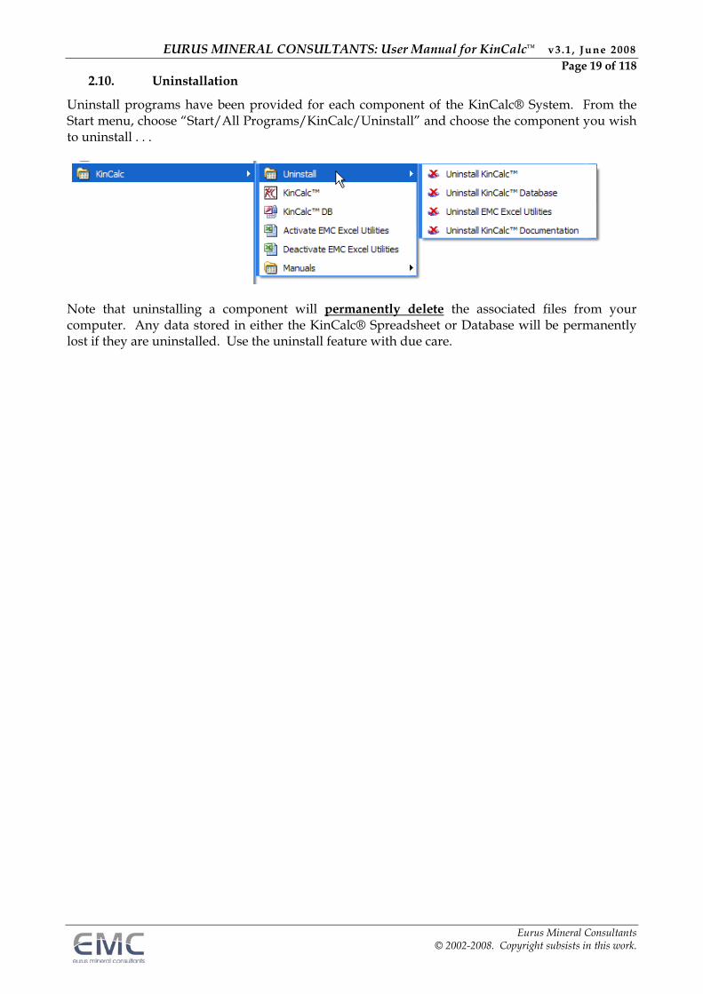
2.10. Uninstallation
Uninstall programs have been provided for each component of the KinCalc® System. From the Start menu, choose “Start/All Programs/KinCalc/Uninstall” and choose the component you wish to uninstall . . .
Note that uninstalling a component will permanently delete the associated files from your computer. Any data stored in either the KinCalc® Spreadsheet or Database will be permanently lost if they are uninstalled. Use the uninstall feature with due care.
EURUS MINERAL CONSULTANTS: User Manual for KinCalc™ v3.1 , June 2008 Page 20 of 118
Eurus Mineral Consultants © 2002-2008. Copyright subsists in this work.
3. IMPORTANT POINTS REGARDING INITIAL SET-UP AND USE OF THE KINCALC®
KINETICS CALCULATOR
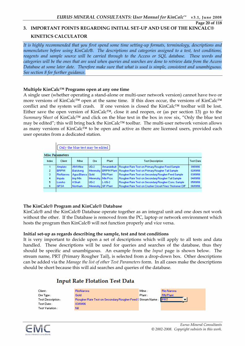
It is highly recommended that you first spend some time setting-up formats, terminology, descriptions and nomenclature before using KinCalc®. The descriptions and categories assigned to a test, test conditions, reagents and sample source will be carried through to the Access or SQL database. These words and categories will be the ones that are used when queries and searches are done to retrieve data from the Access Database at some later date. Therefore make sure that what is used is simple, consistent and unambiguous. See section 8 for further guidance. Multiple KinCalc™ Programs open at any one time A single user (whether operating a stand-alone or multi-user network version) cannot have two or more versions of KinCalc™ open at the same time. If this does occur, the versions of KinCalc™ conflict and the system will crash. If one version is closed the KinCalc™ toolbar will be lost. Either save the open version of KinCalc™, close it and reopen, or (as per section 13) go to the Summary Sheet of KinCalc™ and click on the blue text in the box in row six, “Only the blue text may be edited”; this will bring back the KinCalc™ toolbar. The multi-user network version allows as many versions of KinCalc™ to be open and active as there are licensed users, provided each user operates from a dedicated station.
The KinCalc® Program and KinCalc® Database KinCalc® and the KinCalc® Database operate together as an integral unit and one does not work without the other. If the Database is removed from the PC, laptop or network environment which hosts the program then KinCalc® will not function properly and vice versa. Initial set-up as regards describing the sample, test and test conditions It is very important to decide upon a set of descriptions which will apply to all tests and data handled. These descriptions will be used for queries and searches of the database, thus they should be specific and unambiguous. An example from the Input page is shown below. The stream name, PRT (Primary Rougher Tail), is selected from a drop-down box. Other descriptions can be added via the Manage the list of other Test Parameters form. In all cases make the descriptions should be short because this will aid searches and queries of the database.
EURUS MINERAL CONSULTANTS: User Manual for KinCalc™ v3.1 , June 2008 Page 21 of 118
Eurus Mineral Consultants © 2002-2008. Copyright subsists in this work.
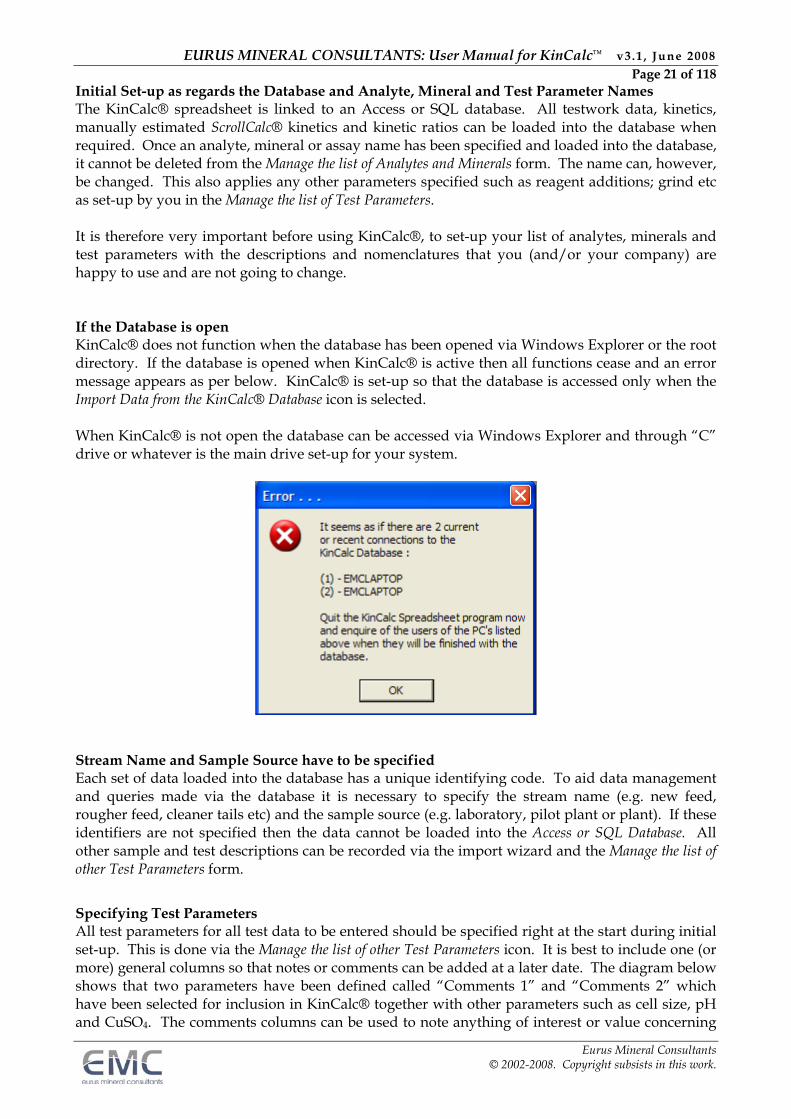
Initial Set-up as regards the Database and Analyte, Mineral and Test Parameter Names The KinCalc® spreadsheet is linked to an Access or SQL database. All testwork data, kinetics, manually estimated ScrollCalc® kinetics and kinetic ratios can be loaded into the database when required. Once an analyte, mineral or assay name has been specified and loaded into the database, it cannot be deleted from the Manage the list of Analytes and Minerals form. The name can, however, be changed. This also applies any other parameters specified such as reagent additions; grind etc as set-up by you in the Manage the list of Test Parameters. It is therefore very important before using KinCalc®, to set-up your list of analytes, minerals and test parameters with the descriptions and nomenclatures that you (and/or your company) are happy to use and are not going to change. If the Database is open KinCalc® does not function when the database has been opened via Windows Explorer or the root directory. If the database is opened when KinCalc® is active then all functions cease and an error message appears as per below. KinCalc® is set-up so that the database is accessed only when the Import Data from the KinCalc® Database icon is selected. When KinCalc® is not open the database can be accessed via Windows Explorer and through “C” drive or whatever is the main drive set-up for your system.
Stream Name and Sample Source have to be specified Each set of data loaded into the database has a unique identifying code. To aid data management and queries made via the database it is necessary to specify the stream name (e.g. new feed, rougher feed, cleaner tails etc) and the sample source (e.g. laboratory, pilot plant or plant). If these identifiers are not specified then the data cannot be loaded into the Access or SQL Database. All other sample and test descriptions can be recorded via the import wizard and the Manage the list of other Test Parameters form.
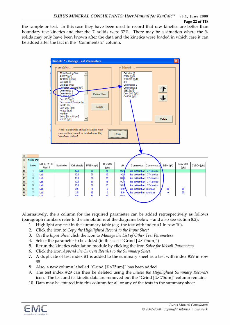
Specifying Test Parameters All test parameters for all test data to be entered should be specified right at the start during initial set-up. This is done via the Manage the list of other Test Parameters icon. It is best to include one (or more) general columns so that notes or comments can be added at a later date. The diagram below shows that two parameters have been defined called “Comments 1” and “Comments 2” which have been selected for inclusion in KinCalc® together with other parameters such as cell size, pH and CuSO4. The comments columns can be used to note anything of interest or value concerning
EURUS MINERAL CONSULTANTS: User Manual for KinCalc™ v3.1 , June 2008 Page 22 of 118
Eurus Mineral Consultants © 2002-2008. Copyright subsists in this work.
the sample or test. In this case they have been used to record that raw kinetics are better than boundary test kinetics and that the % solids were 37%. There may be a situation where the % solids may only have been known after the data and the kinetics were loaded in which case it can be added after the fact in the “Comments 2” column.
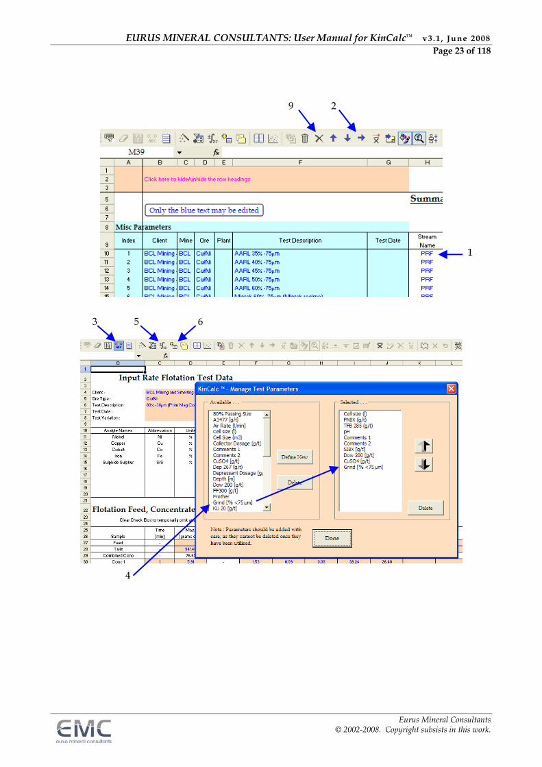
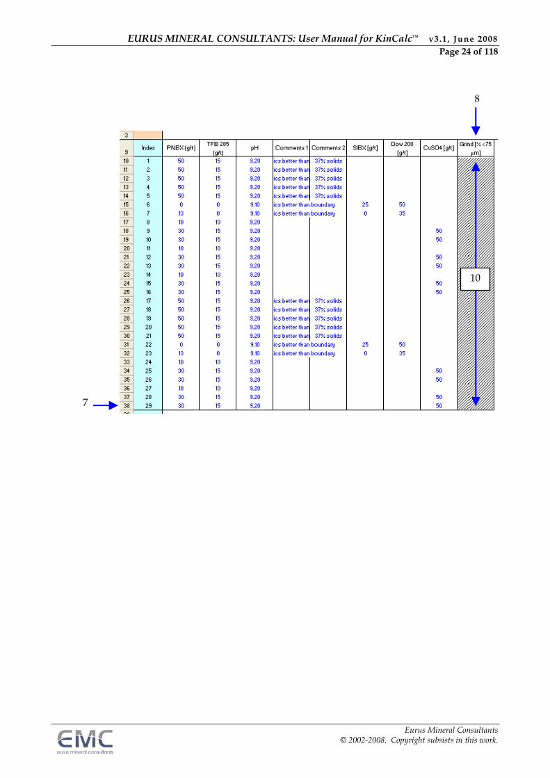
Alternatively, the a column for the required parameter can be added retrospectively as follows (paragraph numbers refer to the annotations of the diagrams below – and also see section 8.2);
1. Highlight any test in the summary table (e.g. the test with index #1 in row 10), 2. Click the icon to Copy the Highlighted Record to the Input Sheet 3. On the Input Sheet click the icon to Manage the List of Other Test Parameters 4. Select the parameter to be added (in this case “Grind [%<75um]”) 5. Rerun the kinetics calculation module by clicking the icon Solve for Kelsall Parameters 6. Click the icon Append the Current Results to the Summary Sheet 7. A duplicate of test index #1 is added to the summary sheet as a test with index #29 in row
38 8. Also, a new column labelled “Grind [%<75um]” has been added 9. The test index #29 can then be deleted using the Delete the Highlighted Summary Record/s
icon. The test and its kinetic data are removed but the “Grind [%<75um]” column remains 10. Data may be entered into this column for all or any of the tests in the summary sheet
EURUS MINERAL CONSULTANTS: User Manual for KinCalc™ v3.1 , June 2008 Page 23 of 118
Eurus Mineral Consultants © 2002-2008. Copyright subsists in this work.
4
2
1
3 6 5
9
EURUS MINERAL CONSULTANTS: User Manual for KinCalc™ v3.1 , June 2008 Page 24 of 118
Eurus Mineral Consultants © 2002-2008. Copyright subsists in this work.
7
8
10
EURUS MINERAL CONSULTANTS: User Manual for KinCalc™ v3.1 , June 2008 Page 25 of 118
Eurus Mineral Consultants © 2002-2008. Copyright subsists in this work.
4. INTRODUCTION TO THE FLOTATION KINETICS CALCULATOR
4.1. What are Flotation Kinetics?
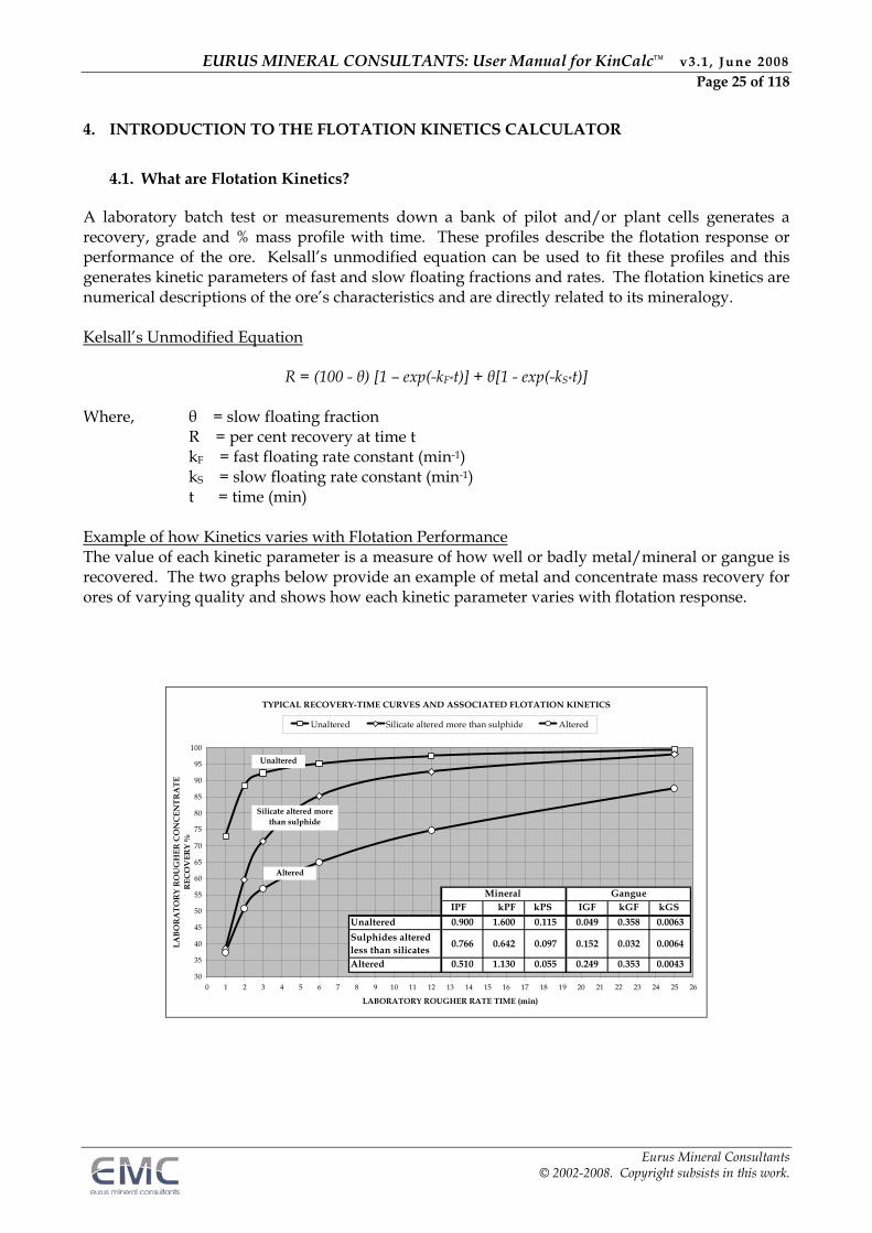
A laboratory batch test or measurements down a bank of pilot and/or plant cells generates a recovery, grade and % mass profile with time. These profiles describe the flotation response or performance of the ore. Kelsall’s unmodified equation can be used to fit these profiles and this generates kinetic parameters of fast and slow floating fractions and rates. The flotation kinetics are numerical descriptions of the ore’s characteristics and are directly related to its mineralogy. Kelsall’s Unmodified Equation
R = (100 - θ) [1 – exp(-kF*t)] + θ[1 - exp(-kS*t)] Where, θ = slow floating fraction
R = per cent recovery at time t kF = fast floating rate constant (min-1) kS = slow floating rate constant (min-1) t = time (min)
Example of how Kinetics varies with Flotation Performance The value of each kinetic parameter is a measure of how well or badly metal/mineral or gangue is recovered. The two graphs below provide an example of metal and concentrate mass recovery for ores of varying quality and shows how each kinetic parameter varies with flotation response.
TYPICAL RECOVERY-TIME CURVES AND ASSOCIATED FLOTATION KINETICS
30
35
40
45
50
55
60
65
70
75
80
85
90
95
100
0 1 2 3 4 5 6 7 8 9 10 11 12 13 14 15 16 17 18 19 20 21 22 23 24 25 26
LABORATORY ROUGHER RATE TIME (min)
LA
BO
RA
TO
RY
RO
UG
HE
R C
ON
CE
NT
RA
TE
R
EC
OV
ER
Y %
Unaltered Silicate altered more than sulphide Altered
Silicate altered more than sulphide
Unaltered
Altered
IPF kPF kPS IGF kGF kGS
Unaltered 0.900 1.600 0.115 0.049 0.358 0.0063
Sulphides altered less than silicates
0.766 0.642 0.097 0.152 0.032 0.0064
Altered 0.510 1.130 0.055 0.249 0.353 0.0043
Mineral Gangue
EURUS MINERAL CONSULTANTS: User Manual for KinCalc™ v3.1 , June 2008 Page 26 of 118
Eurus Mineral Consultants © 2002-2008. Copyright subsists in this work.
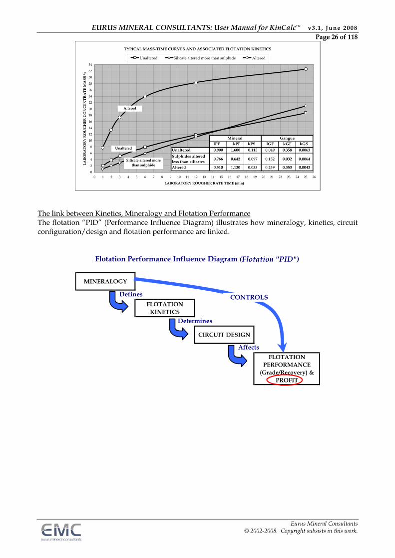
TYPICAL MASS-TIME CURVES AND ASSOCIATED FLOTATION KINETICS
0
2
4
6
8
10
12
14
16
18
20
22
24
26
28
30
32
34
0 1 2 3 4 5 6 7 8 9 10 11 12 13 14 15 16 17 18 19 20 21 22 23 24 25 26
LABORATORY ROUGHER RATE TIME (min)
LA
BO
RA
TO
RY
RO
UG
HE
R C
ON
CE
NT
RA
TE
MA
SS
%
Unaltered Silicate altered more than sulphide Altered
Silicate altered more than sulphide
Unaltered
Altered
IPF kPF kPS IGF kGF kGS
Unaltered 0.900 1.600 0.115 0.049 0.358 0.0063
Sulphides altered less than silicates
0.766 0.642 0.097 0.152 0.032 0.0064
Altered 0.510 1.130 0.055 0.249 0.353 0.0043
Mineral Gangue
The link between Kinetics, Mineralogy and Flotation Performance The flotation “PID” (Performance Influence Diagram) illustrates how mineralogy, kinetics, circuit configuration/design and flotation performance are linked.
MINERALOGY
FLOTATION KINETICS
CIRCUIT DESIGN
FLOTATION PERFORMANCE
(Grade/Recovery) & PROFIT
Flotation Performance Influence Diagram (Flotation "PID")
Determines
Affects
Defines CONTROLS

EURUS MINERAL CONSULTANTS: User Manual for KinCalc™ v3.1 , June 2008 Page 27 of 118
Eurus Mineral Consultants © 2002-2008. Copyright subsists in this work.
4.2. Terminology and Acronyms
Elements, whether metal or non-metal are referred to as analytes. An assay is a measure of concentration of an analyte in percent or grams per tonne. Various acronyms and descriptions are used as detailed in the table below. Note that the table has been compiled with reference to Nickel;
Acronym Meaning INiF = Fast floating fraction of Nickel kNiF = Fast floating rate of Nickel kNiS = Slow floating rate of Nickel
FFR = Fast Floating Ratio (INiF/IGF), the fast floating flotation fraction of Nickel relative to gangue
SFR = Slow Floating Ratio (kNiS/kGS), the slow floating flotation rate of Nickel relative to gangue
Nickel Floatability
= A measure of the floatability of Nickel incorporating the two most important parameters which influence recovery and grade (INiF*kNiS)*1000
Nickel Full Floatability
= A measure of the floatability of Nickel incorporating all three fraction and rate parameters (INiF*kNiF*kNiS)*1000
Gangue Floatability =
A measure of the floatability of the gangue component (IGF*kGS)*1000
Gangue Full Floatability
= A measure of the floatability of gangue incorporating all three fraction and rate parameters (IGF*kGF*kGS)*1000
Selectivity = A measure of relative floatability of metal or mineral to gangue incorporating all kinetic values. For example, Nickel selectivity is defined as [(INiF*kNiF*kNiS)/(IGF*kGF*kGS)]*1000
In all cases, I = fraction; k = rate, F = fast and S = slow Ni = Nickel and this can substituted as required depending on what is being analysed or assayed.
A few examples are, P or PGM is substituted for Platinum Group Metals, Cu for Copper, Co for Cobalt, Au for Gold, S for Sulphur, MgO for Magnesium Oxide, Cp for Chalcopyrite, Pn for Pentlandite, Po for Pyrrhotite, G for Gangue and M for Mass Met and Min for any metal or mineral.
4.3. Brief Overview of the Kinetics Calculator
The Kinetics Calculator, 1. Allows minerals, analytes, assays and their units of measurement to be managed, 2. Allows other test and measurement parameters and their units of measurement to be
managed, 3. Permits formats to be specified for data collection from other excel files and
worksheets, 4. Permits all test data and test descriptions to be recorded, 5. Allows test stream names and source (i.e. lab, pilot plant or plant) to be recorded,
EURUS MINERAL CONSULTANTS: User Manual for KinCalc™ v3.1 , June 2008 Page 28 of 118
Eurus Mineral Consultants © 2002-2008. Copyright subsists in this work.
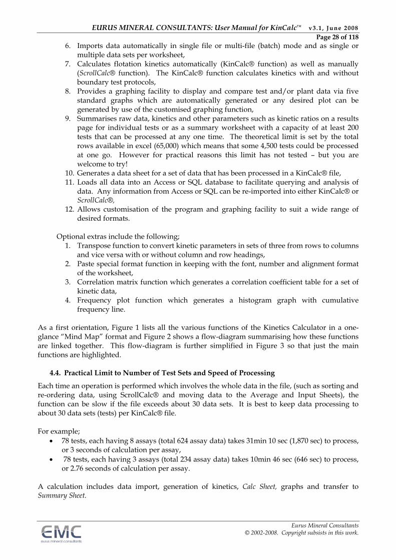
6. Imports data automatically in single file or multi-file (batch) mode and as single or multiple data sets per worksheet,
7. Calculates flotation kinetics automatically (KinCalc® function) as well as manually (ScrollCalc® function). The KinCalc® function calculates kinetics with and without boundary test protocols,
8. Provides a graphing facility to display and compare test and/or plant data via five standard graphs which are automatically generated or any desired plot can be generated by use of the customised graphing function,
9. Summarises raw data, kinetics and other parameters such as kinetic ratios on a results page for individual tests or as a summary worksheet with a capacity of at least 200 tests that can be processed at any one time. The theoretical limit is set by the total rows available in excel (65,000) which means that some 4,500 tests could be processed at one go. However for practical reasons this limit has not tested – but you are welcome to try!
10. Generates a data sheet for a set of data that has been processed in a KinCalc® file, 11. Loads all data into an Access or SQL database to facilitate querying and analysis of
data. Any information from Access or SQL can be re-imported into either KinCalc® or ScrollCalc®,
12. Allows customisation of the program and graphing facility to suit a wide range of desired formats.
Optional extras include the following;
1. Transpose function to convert kinetic parameters in sets of three from rows to columns and vice versa with or without column and row headings,
2. Paste special format function in keeping with the font, number and alignment format of the worksheet,
3. Correlation matrix function which generates a correlation coefficient table for a set of kinetic data,
4. Frequency plot function which generates a histogram graph with cumulative frequency line.
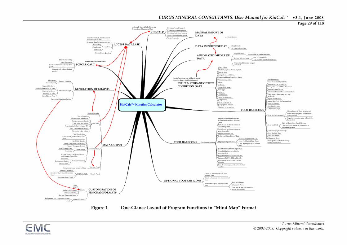
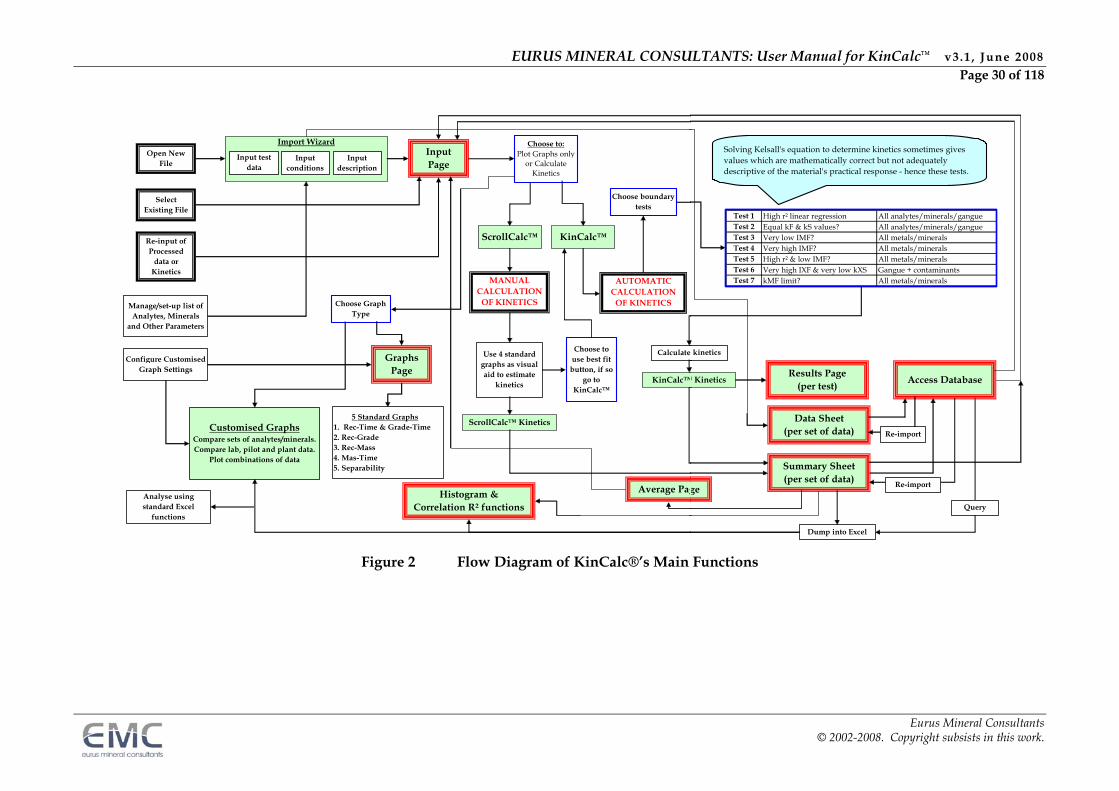
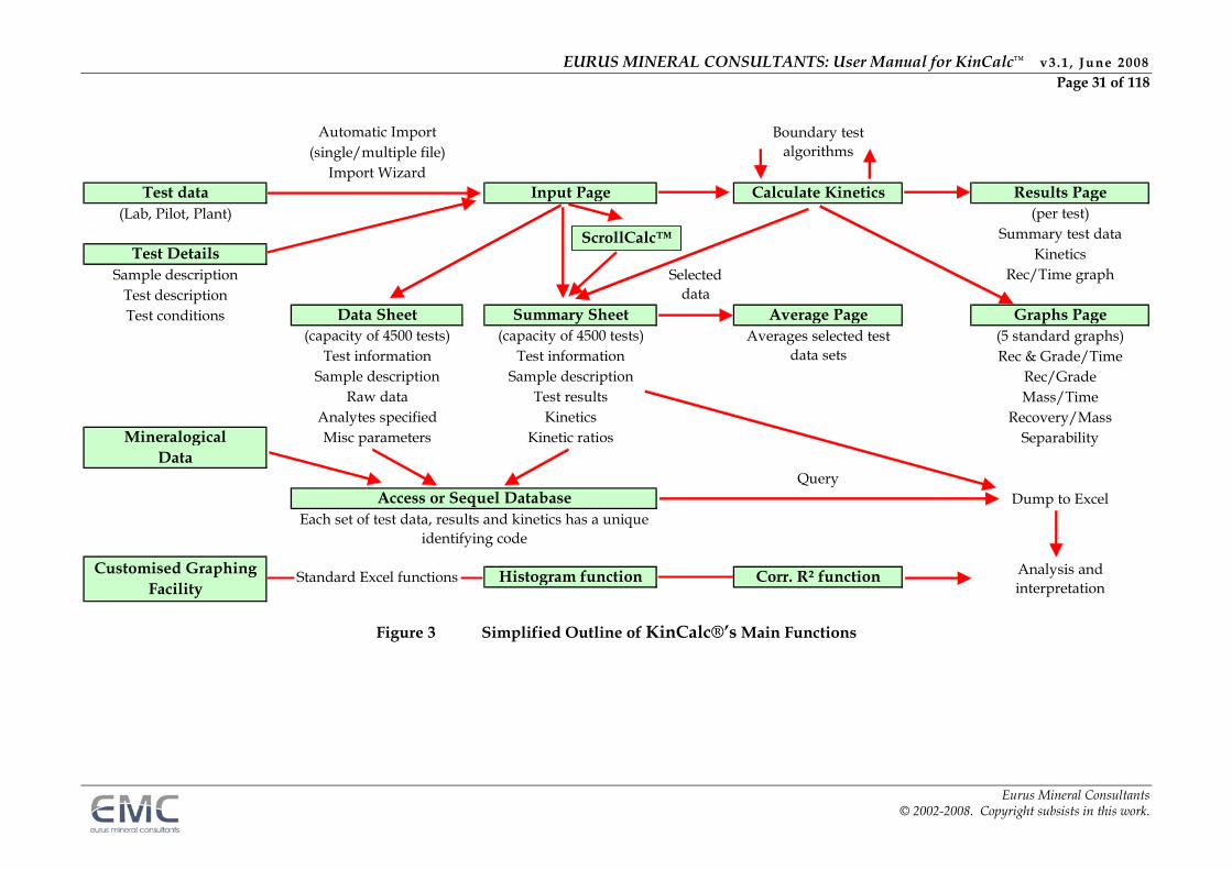
As a first orientation, Figure 1 lists all the various functions of the Kinetics Calculator in a one-glance “Mind Map” format and Figure 2 shows a flow-diagram summarising how these functions are linked together. This flow-diagram is further simplified in Figure 3 so that just the main functions are highlighted.
4.4. Practical Limit to Number of Test Sets and Speed of Processing
Each time an operation is performed which involves the whole data in the file, (such as sorting and re-ordering data, using ScrollCalc® and moving data to the Average and Input Sheets), the function can be slow if the file exceeds about 30 data sets. It is best to keep data processing to about 30 data sets (tests) per KinCalc® file. For example;
78 tests, each having 8 assays (total 624 assay data) takes 31min 10 sec (1,870 sec) to process, or 3 seconds of calculation per assay,
78 tests, each having 3 assays (total 234 assay data) takes 10min 46 sec (646 sec) to process, or 2.76 seconds of calculation per assay.
A calculation includes data import, generation of kinetics, Calc Sheet, graphs and transfer to Summary Sheet.
EURUS MINERAL CONSULTANTS: User Manual for KinCalc™ v3.1 , June 2008 Page 29 of 118
Eurus Mineral Consultants © 2002-2008. Copyright subsists in this work.
KIN-CALC
GENERATION OF GRAPHS
MANUAL IMPORT OF DATA
SCROLL-CALC
ACCESS DATABASE
AUTOMATIC IMPORT OF DATA
DATA IMPORT FORMAT
INPUT & STORAGE OF TEST CONDITION DATA
DATA OUTPUT
CUSTOMISATION OF PROGRAM FORMATS
TOOL BAR ICONS
OPTIONAL TOOLBAR ICONS
TOOL BAR ICONS
KinCalc™ Kinetics Calculator
Kinetics of metal/mineral
Kinetics of floatable gangue
Kinetics of entrained material
With/without boundary tests
What-if scenarios
Custom FunctionsHistogram
Correlation r2
5 Standard Graphs
Separability Curve
Recovery and Grade vs Time
Recovery vs Grade
Recovery vs Mass
Conc Mass vs Time
Customised Graphing Facility
Single data set
Educational facility
What-if scenarios
Kinetics estimation with few data points
Compare lab, pilot and plant profiles
Import of KinCalc, ScrollCalc and Test Description Data
Re-import data for further analysis
AnalysisData sorting
Correlations
Statistical
Generation of Queries Single file basis Any number of Data Worksheets
Batch of files in a folderAny number of Files
Any Number of Data Worksheets
Single or multiple data sets per worksheet
Set-up formats
Lab, Pilot or Plant data
Client/Mine
Ore body/type or stream in plant
Date or time
Reagents and additions
Reagent addition Straight or Staged
Conditioning Time
Grind
% Solids
Power (kW) input
Cell Type
Cell rpm
Air Flowrate
Water Type/Quality
Temperature
Eh, pH, Oxygen %
Geographical position
Depth or other position
Standard Graphs
Data Sheet
Test information
Miscellaneous parameters
Analyte names and units
Conc times and masses
Analytes selected and category IDs
Feed, Tails and Conc assays
Parameter order indices
Summary Sheet
Test Descriptions
Kinetics with/without Boundary Tests
ScrollCalc Kinetics
Linear Flag (Mass-Time Curve)
Sum of the squared errors
Kinetic RatiosSlow Floating Ratio
Selectivity
Kinetic Measure of Metal/Mineral and Gangue Floatability
Test Data SummaryRecoveries
Concentrate Grades
Head Grades
Average PageCalculates average for a set of data
Results PageSingle A4 page
Test Data Summary
Kinetics with/without Boundary Tests
Recovery-Time Graph
Graphs
Font
Type
Markers (12 options)
Lines (12 options)
Size and Dimension Ratio
General ProgramBackground and foreground colours
Font
Goto Input page
Clear the current Input Data
Manage the List of Analytes
Manage the List of Other Parameters
Manage Stream Names
Add current data to the Summary Sheet
Copy current sheet/page to a new workbook
Import Data Wizard
Import data from KinCalc database
Solve for Kinetics
Goto Results page
Goto Graphs page
Go to the Average sheet
Clear all data off the Average sheet
Delete the highlighted record on the Average sheet
Copy the current average values to the Input sheet
Go to ScrollCalcClear all data off the ScrollCalc page
Copy the active ScrollCalc parameters to the Summary sheet
Customise program settings
Show the Data sheet
Rows to Columns
Columns to Rows
Paste special function maintaing format of worksheet
Create a Correlation Matrix from selected data
Create a Frquency plot from selected data
Transform Layout of Kinetic Data Sets
Rows to Columns
Columns to Rows
Paste special function maintaing format of worksheet
Goto Summary sheet
Highlight Differences between Kinetics with/without Boundary Tests
Sort all data in chosen column in descending order
Sort all data in chosen column in ascending order
Highlight specific row
Delete highlighted row of data
Highlight a Specific Row
Move Highlighted Row Up
Move Highlighted Row Down
Copy Highlighted Row to Input Sheet
Clear Summary Sheet & Input Page
Copy highlighted record to the Average sheet
Copy highlighted row to ScrollCalc
Summary Roll-Up: Hide all details
Post current record to the KinCalc database
Post all summary records to the KinCalc database
Automatic Import, Calculation and Generation of Summary Sheet
Manual calculation of kinetics
Input of anything user wishes to record; examples shown for illustration only
Figure 1 One-Glance Layout of Program Functions in “Mind Map” Format
EURUS MINERAL CONSULTANTS: User Manual for KinCalc™ v3.1 , June 2008 Page 30 of 118
Eurus Mineral Consultants © 2002-2008. Copyright subsists in this work.
Import WizardOpen New
File
Select Existing File
Re-input of Processed
data or Kinetics
Input test data
Input conditions
Input description
Input Page
Choose to:Plot Graphs only
or Calculate Kinetics
ScrollCalc™ KinCalc™
MANUAL CALCULATION
OF KINETICS
AUTOMATIC CALCULATION
OF KINETICSManage/set-up list of Analytes, Minerals
and Other Parameters
Configure Customised Graph Settings
Use 4 standard graphs as visual aid to estimate
kinetics
ScrollCalc™ Kinetics
Choose to use best fit
button, if so go to
KinCalc™
Calculate
KinCalc™
Choose boundary tests
Graphs Page
Choose Graph Type
5 Standard Graphs1. Rec-Time & Grade-Time2. Rec-Grade3. Rec-Mass4. Mas-Time5. Separability
Customised GraphsCompare sets of analytes/minerals. Compare lab, pilot and plant data.
Plot combinations of data
Average PagHistogram & Correlation R² functions
Analyse using standard Excel
functions
Test 1 High r² linear regression All analytes/minerals/gangueTest 2 Equal kF & kS values? All analytes/minerals/gangueTest 3 Very low IMF? All metals/mineralsTest 4 Very high IMF? All metals/mineralsTest 5 High r² & low IMF? All metals/mineralsTest 6 Very high IXF & very low kXS Gangue + contaminantsTest 7 kMF limit? All metals/minerals
Solving Kelsall's equation to determine kinetics sometimes gives values which are mathematically correct but not adequately descriptive of the material's practical response - hence these tests.
kinetics
™ Kinetics
Summary Sheet (per set of data)
Results Page (per test)
Data Sheet (per set of data)
Access Database
Re-import
Re-import
Dump into Excel
Query
ge
Figure 2 Flow Diagram of KinCalc®’s Main Functions
EURUS MINERAL CONSULTANTS: User Manual for KinCalc™ v3.1 , June 2008 Page 31 of 118
Eurus Mineral Consultants © 2002-2008. Copyright subsists in this work.
Automatic Import(single/multiple file)
Import WizardTest data Input Page Calculate Kinetics Results Page
(Lab, Pilot, Plant) (per test)Summary test data
Test Details KineticsSample description Rec/Time graph
Test descriptionTest conditions Data Sheet Summary Sheet Average Page Graphs Page
(capacity of 4500 tests) (capacity of 4500 tests) (5 standard graphs)Test information Test information Rec & Grade/Time
Sample description Sample description Rec/GradeRaw data Test results Mass/Time
Analytes specified Kinetics Recovery/MassMisc parameters Kinetic ratios Separability
QueryDump to Excel
Standard Excel functions Histogram function Corr. R² function Analysis and interpretation
Access or Sequel DatabaseEach set of test data, results and kinetics has a unique
identifying code
Mineralogical Data
Customised Graphing Facility
Selected data
Boundary test algorithms
Averages selected test data sets
ScrollCalc™
Figure 3 Simplified Outline of KinCalc®’s Main Functions
EURUS MINERAL CONSULTANTS: User Manual for KinCalc™ v3.1 , June 2008 Page 32 of 118
Eurus Mineral Consultants © 2002-2008. Copyright subsists in this work.
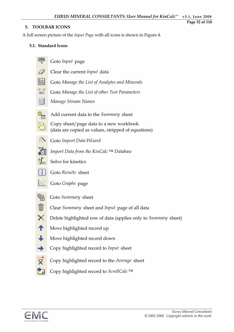
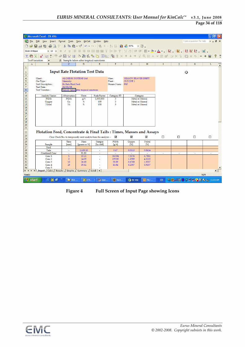
5. TOOLBAR ICONS
A full screen picture of the Input Page with all icons is shown in Figure 4.
5.1. Standard Icons
Goto Input page
Clear the current Input data
Goto Manage the List of Analytes and Minerals
Goto Manage the List of other Test Parameters
Manage Stream Names
Add current data to the Summary sheet
Copy sheet/page data to a new workbook (data are copied as values, stripped of equations)
Goto Import Data Wizard
Import Data from the KinCalc ™ Database
Solve for kinetics
Goto Results sheet
Goto Graphs page
Goto Summary sheet
Clear Summary sheet and Input page of all data
Delete highlighted row of data (applies only to Summary sheet)
Move highlighted record up
Move highlighted record down
Copy highlighted record to Input sheet
Copy highlighted record to the Average sheet
Copy highlighted record to ScrollCalc ™
EURUS MINERAL CONSULTANTS: User Manual for KinCalc™ v3.1 , June 2008 Page 33 of 118
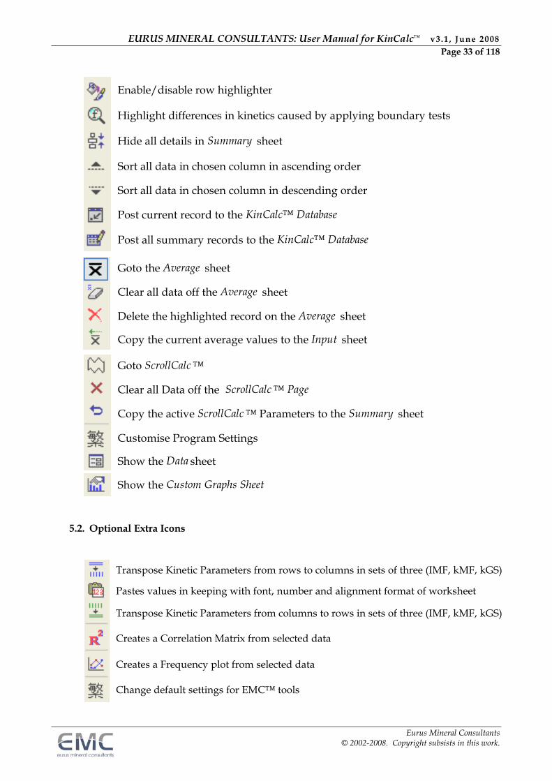
Eurus Mineral Consultants © 2002-2008. Copyright subsists in this work.
Enable/disable row highlighter
Highlight differences in kinetics caused by applying boundary tests
Hide all details in Summary sheet
Sort all data in chosen column in ascending order
Sort all data in chosen column in descending order
Post current record to the KinCalc™ Database
Post all summary records to the KinCalc™ Database
Goto the Average sheet
Clear all data off the Average sheet
Delete the highlighted record on the Average sheet
Copy the current average values to the Input sheet
Goto ScrollCalc ™
Clear all Data off the ScrollCalc ™ Page
Copy the active ScrollCalc ™ Parameters to the Summary sheet
Customise Program Settings
Show the Data sheet
Show the Custom Graphs Sheet
5.2. Optional Extra Icons
Transpose Kinetic Parameters from rows to columns in sets of three (IMF, kMF, kGS)
Pastes values in keeping with font, number and alignment format of worksheet
Transpose Kinetic Parameters from columns to rows in sets of three (IMF, kMF, kGS)
Creates a Correlation Matrix from selected data
Creates a Frequency plot from selected data
Change default settings for EMC™ tools
EURUS MINERAL CONSULTANTS: User Manual for KinCalc™ v3.1 , June 2008 Page 34 of 118
Eurus Mineral Consultants © 2002-2008. Copyright subsists in this work.
Figure 4 Full Screen of Input Page showing Icons
EURUS MINERAL CONSULTANTS: User Manual for KinCalc™ v3.1 , June 2008 Page 35 of 118
Eurus Mineral Consultants © 2002-2008. Copyright subsists in this work.
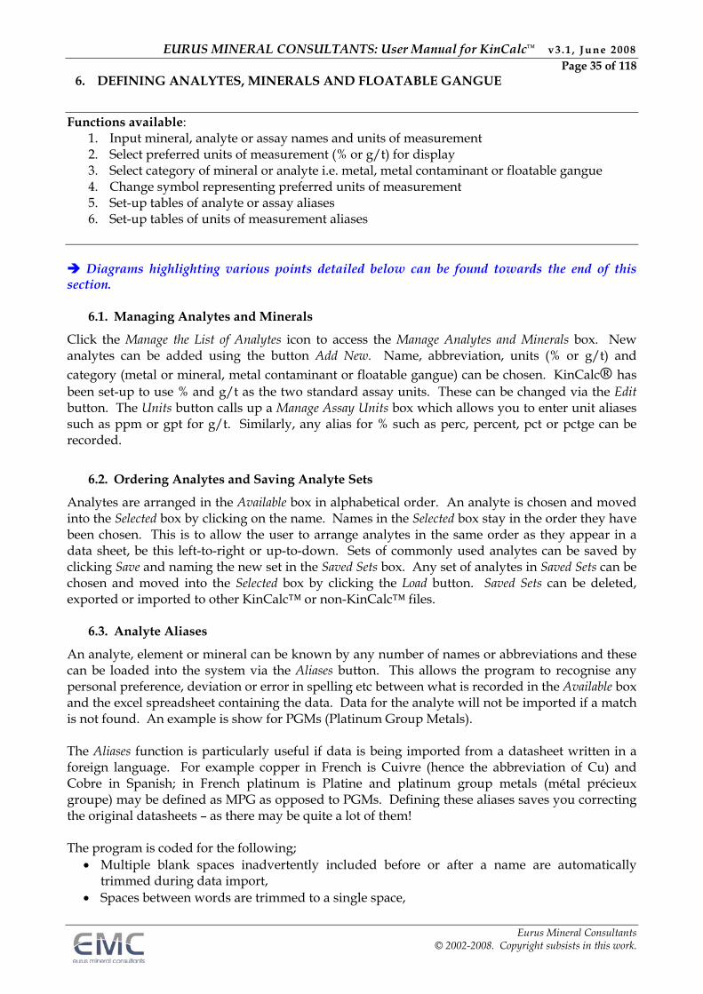
6. DEFINING ANALYTES, MINERALS AND FLOATABLE GANGUE
Functions available:
1. Input mineral, analyte or assay names and units of measurement 2. Select preferred units of measurement (% or g/t) for display 3. Select category of mineral or analyte i.e. metal, metal contaminant or floatable gangue 4. Change symbol representing preferred units of measurement 5. Set-up tables of analyte or assay aliases 6. Set-up tables of units of measurement aliases
Diagrams highlighting various points detailed below can be found towards the end of this section.
6.1. Managing Analytes and Minerals
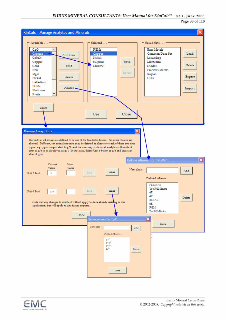
Click the Manage the List of Analytes icon to access the Manage Analytes and Minerals box. New analytes can be added using the button Add New. Name, abbreviation, units (% or g/t) and category (metal or mineral, metal contaminant or floatable gangue) can be chosen. KinCalc® has been set-up to use % and g/t as the two standard assay units. These can be changed via the Edit button. The Units button calls up a Manage Assay Units box which allows you to enter unit aliases such as ppm or gpt for g/t. Similarly, any alias for % such as perc, percent, pct or pctge can be recorded.
6.2. Ordering Analytes and Saving Analyte Sets
Analytes are arranged in the Available box in alphabetical order. An analyte is chosen and moved into the Selected box by clicking on the name. Names in the Selected box stay in the order they have been chosen. This is to allow the user to arrange analytes in the same order as they appear in a data sheet, be this left-to-right or up-to-down. Sets of commonly used analytes can be saved by clicking Save and naming the new set in the Saved Sets box. Any set of analytes in Saved Sets can be chosen and moved into the Selected box by clicking the Load button. Saved Sets can be deleted, exported or imported to other KinCalc™ or non-KinCalc™ files.
6.3. Analyte Aliases
An analyte, element or mineral can be known by any number of names or abbreviations and these can be loaded into the system via the Aliases button. This allows the program to recognise any personal preference, deviation or error in spelling etc between what is recorded in the Available box and the excel spreadsheet containing the data. Data for the analyte will not be imported if a match is not found. An example is show for PGMs (Platinum Group Metals). The Aliases function is particularly useful if data is being imported from a datasheet written in a foreign language. For example copper in French is Cuivre (hence the abbreviation of Cu) and Cobre in Spanish; in French platinum is Platine and platinum group metals (métal précieux groupe) may be defined as MPG as opposed to PGMs. Defining these aliases saves you correcting the original datasheets – as there may be quite a lot of them! The program is coded for the following;
Multiple blank spaces inadvertently included before or after a name are automatically trimmed during data import,
Spaces between words are trimmed to a single space,
EURUS MINERAL CONSULTANTS: User Manual for KinCalc™ v3.1 , June 2008 Page 36 of 118
Eurus Mineral Consultants © 2002-2008. Copyright subsists in this work.
The same words with and without a space in between are not recognised. Hence TotPGM&Au must be specified as well as Tot PGM&Au as per the example,
Upper and lower case are recognised in any combination, e.g. Tot PGM&Au and Tot PgM&au
Any alias found in a datasheet will be imported as its preferred record (as set-up in section 6.1 above), e.g. ppm and gpt are imported as g/t, and copper, Cu, cu and any other aliases defined are imported as Copper. Note that if units of % have been chosen as the preferred unit of measure, then all data as g/t or ppm will be automatically imported as %. If this needs to be changed then go to section 6.5.
6.4. Setting Your Own Symbol or Acronym for a Standard Assay Unit
KinCalc® has been set-up with two standard assay units being % and g/t. If you want to change these and use your own symbol, name or acronym then any one of the two standard units can be changed by clicking the Units button of the Manage Analytes and Minerals box. This brings up the Manage Assay Units box. Unit 2 Text denotes 10^2 and defines % as the default assay unit in the Current Value column, Unit 6 Text denotes 10^6 and defines g/t as the default assay unit also in the Current Value column. Enter the symbol, name or acronym you want to use into the appropriate box in the New Value column. If the new value also occurs as one of the assay aliases then you will be prompted to delete this from the assay alias box.
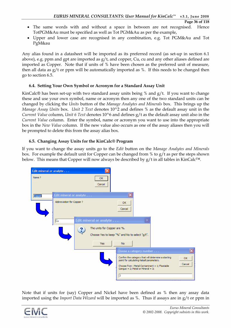
6.5. Changing Assay Units for the KinCalc® Program
If you want to change the assay units go to the Edit button on the Manage Analytes and Minerals box. For example the default unit for Copper can be changed from % to g/t as per the steps shown below. This means that Copper will now always be described by g/t in all tables in KinCalc™. Note that if units for (say) Copper and Nickel have been defined as % then any assay data imported using the Import Data Wizard will be imported as %. Thus if assays are in g/t or ppm in
EURUS MINERAL CONSULTANTS: User Manual for KinCalc™ v3.1 , June 2008 Page 37 of 118
Eurus Mineral Consultants © 2002-2008. Copyright subsists in this work.
the raw data sheet, the values will be imported as %. Similarly if the units have been defined as g/t or ppm, then all g/t, ppm and % data associated with that analyte will be imported as g/t or ppm (which ever one has been chosen).
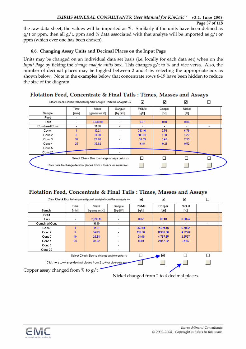
6.6. Changing Assay Units and Decimal Places on the Input Page
Units may be changed on an individual data set basis (i.e. locally for each data set) when on the Input Page by ticking the change analyte units box. This changes g/t to % and vice versa. Also, the number of decimal places may be toggled between 2 and 4 by selecting the appropriate box as shown below. Note in the examples below that concentrate rows 6-19 have been hidden to reduce the size of the diagram.
Copper assay changed from % to g/t Nickel changed from 2 to 4 decimal places
EURUS MINERAL CONSULTANTS: User Manual for KinCalc™ v3.1 , June 2008 Page 38 of 118
Eurus Mineral Consultants © 2002-2008. Copyright subsists in this work.
EURUS MINERAL CONSULTANTS: User Manual for KinCalc™ v3.1 , June 2008 Page 39 of 118
Eurus Mineral Consultants © 2002-2008. Copyright subsists in this work.
6.7. Determining the Category of an Analyte
The categories and codes used to describe an analyte are shown in the table below. Floatable material is categorised and assigned a code in order to apply the appropriate protocol when calculating kinetics.
Analyte Code Description Metal Contaminant 1 Non-economic metal element or mineral Floatable Gangue 2 Non-economic element or mineral Metal or Mineral 3 Economic metal element or mineral
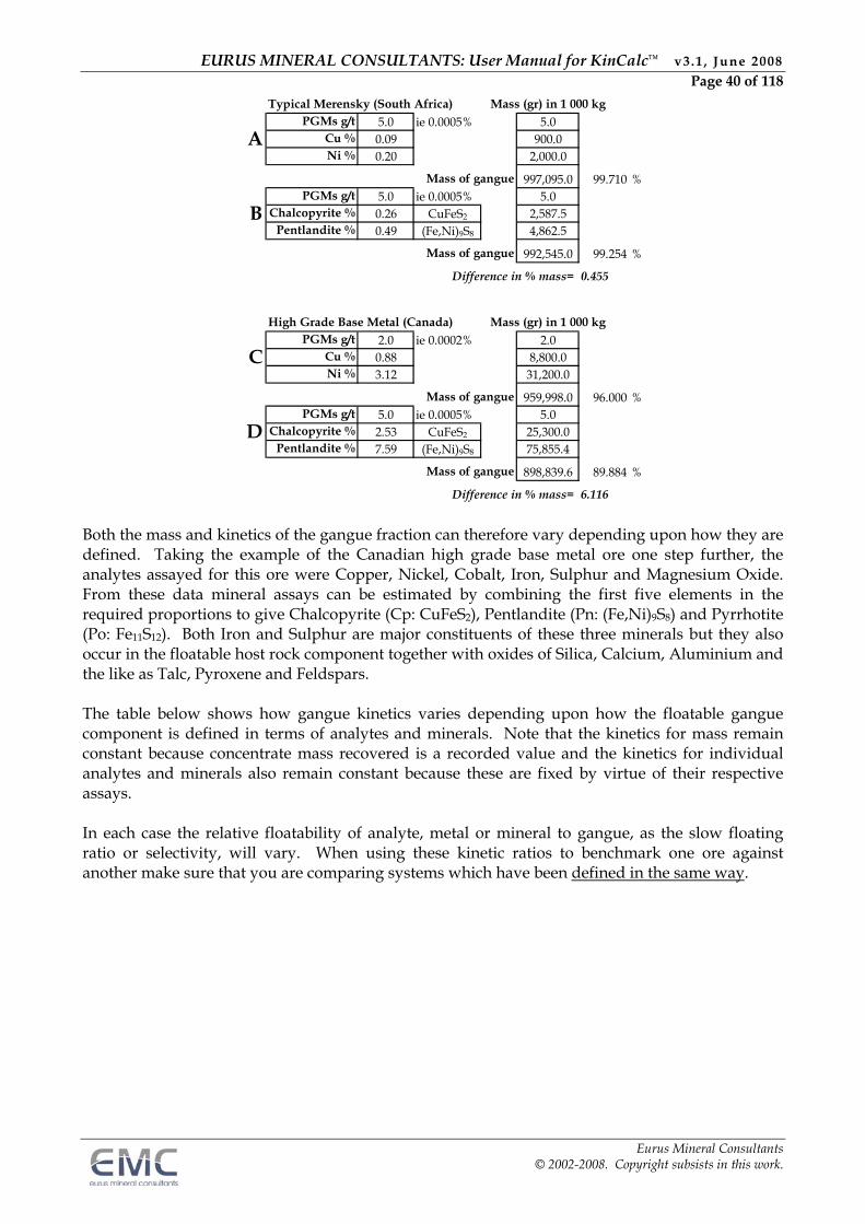
Metal contaminants are non valuable material (or metals) which are recovered as a by-product of the flotation process. Recovery may be by entrainment, solid solution or attachment to floatable gangue or mineral because of poor liberation. Examples are Iron and Chromium in the form of Chromitite (FeCr2O3), Magnesium and Manganese. Floatable gangue is defined as non valuable material recovered to concentrate and is the difference between total concentrate mass and the total mass of assayed elements and/or minerals. Typically, floatable gangue consists of common host rock minerals such as Talc H2Mg3(SiO3)4; Pyroxene, Ca(Mg,Fe)(SiO3)2; and any of the Feldspars, e.g. Anorthite CaAl2Si2O8. Sulphur is not usually contained in a typical gangue mineral but if it is, it is usually as a sulphate e.g. Polyhalite 2CaSO4·MgSO4·K2SO4. If water recovery is measured it is categorised as floatable gangue for the purposes of the KinCalc® program. Metal or Mineral is any economic material. What Constitutes Floatable Gangue? This can be tricky depending on how the economic metals occur in the ore and whether you choose to follow flotation response in terms of pure metal or mineral. All scenarios presented below are correct and depend upon how floatable gangue is defined. It does not matter which definition or view is taken as long as the preferred one is consistently used. For example the table below compares a Platinum-bearing Merensky ore with a high grade base metal ore from Canada. For Merensky ore, defining floatable gangue in terms of metals or minerals makes only a 0.455% difference whereas it makes a 6.116% difference for the Canadian ore. Merensky cases “A” and “B” produce very similar gangue kinetics, but Canadian ore cases “C” and “D” produce kinetics which are significantly different. In each case, both sets of kinetics (A and B) and (C and D) are equally correct descriptions of their particular systems.
EURUS MINERAL CONSULTANTS: User Manual for KinCalc™ v3.1 , June 2008 Page 40 of 118
Eurus Mineral Consultants © 2002-2008. Copyright subsists in this work.
Typical Merensky (South Africa) Mass (gr) in 1 000 kgPGMs g/t 5.0 ie 0.0005% 5.0
Cu % 0.09 900.0Ni % 0.20 2,000.0
Mass of gangue 997,095.0 99.710 %PGMs g/t 5.0 ie 0.0005% 5.0
Chalcopyrite % 0.26 CuFeS2 2,587.5Pentlandite % 0.49 (Fe,Ni)9S8 4,862.5
Mass of gangue 992,545.0 99.254 %
Difference in % mass= 0.455
High Grade Base Metal (Canada) Mass (gr) in 1 000 kgPGMs g/t 2.0 ie 0.0002% 2.0
Cu % 0.88 8,800.0Ni % 3.12 31,200.0
Mass of gangue 959,998.0 96.000 %PGMs g/t 5.0 ie 0.0005% 5.0
Chalcopyrite % 2.53 CuFeS2 25,300.0Pentlandite % 7.59 (Fe,Ni)9S8 75,855.4
Mass of gangue 898,839.6 89.884 %
Difference in % mass= 6.116
C
B
D
A
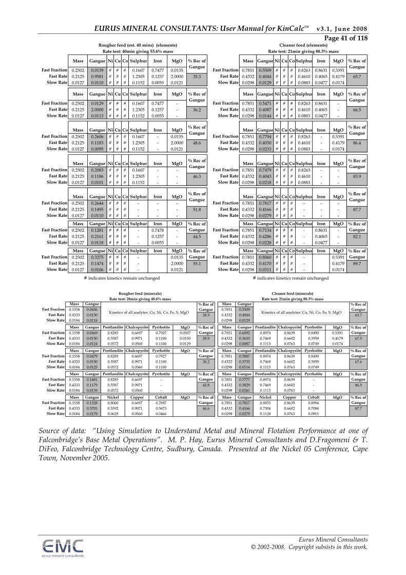
Both the mass and kinetics of the gangue fraction can therefore vary depending upon how they are defined. Taking the example of the Canadian high grade base metal ore one step further, the analytes assayed for this ore were Copper, Nickel, Cobalt, Iron, Sulphur and Magnesium Oxide. From these data mineral assays can be estimated by combining the first five elements in the required proportions to give Chalcopyrite (Cp: CuFeS2), Pentlandite (Pn: (Fe,Ni)9S8) and Pyrrhotite (Po: Fe11S12). Both Iron and Sulphur are major constituents of these three minerals but they also occur in the floatable host rock component together with oxides of Silica, Calcium, Aluminium and the like as Talc, Pyroxene and Feldspars. The table below shows how gangue kinetics varies depending upon how the floatable gangue component is defined in terms of analytes and minerals. Note that the kinetics for mass remain constant because concentrate mass recovered is a recorded value and the kinetics for individual analytes and minerals also remain constant because these are fixed by virtue of their respective assays. In each case the relative floatability of analyte, metal or mineral to gangue, as the slow floating ratio or selectivity, will vary. When using these kinetic ratios to benchmark one ore against another make sure that you are comparing systems which have been defined in the same way.
EURUS MINERAL CONSULTANTS: User Manual for KinCalc™ v3.1 , June 2008 Page 41 of 118
Eurus Mineral Consultants © 2002-2008. Copyright subsists in this work.
Mass Gangue Ni Cu Co Sulphur Iron MgO Mass Gangue Ni Cu Co Sulphur Iron MgO
Fast Fraction 0.2502 0.0139 # # # 0.1607 0.7477 0.0135 Fast Fraction 0.7851 0.5509 # # # 0.8263 0.8631 0.5391Fast Rate 0.2125 0.9581 # # # 1.2305 0.1257 2.0000 35.3 Fast Rate 0.4332 0.4044 # # # 0.4610 0.4065 0.4179 65.7
Slow Rate 0.0127 0.0110 # # # 0.1152 0.0055 0.0121 Slow Rate 0.0298 0.0129 # # # 0.0883 0.0477 0.0174
Mass Gangue Ni Cu Co Sulphur Iron MgO Mass Gangue Ni Cu Co Sulphur Iron MgO
Fast Fraction 0.2502 0.0129 # # # 0.1607 0.7477 - Fast Fraction 0.7851 0.5471 # # # 0.8263 0.8631 -Fast Rate 0.2125 2.0000 # # # 1.2305 0.1257 - 36.2 Fast Rate 0.4332 0.4087 # # # 0.4610 0.4065 - 66.5
Slow Rate 0.0127 0.0113 # # # 0.1152 0.0055 - Slow Rate 0.0298 0.0144 # # # 0.0883 0.0477 -
Mass Gangue Ni Cu Co Sulphur Iron MgO Mass Gangue Ni Cu Co Sulphur Iron MgOFast Fraction 0.2502 0.2606 # # # 0.1607 - 0.0135 Fast Fraction 0.7851 0.7794 # # # 0.8263 - 0.5391
Fast Rate 0.2125 0.1183 # # # 1.2305 - 2.0000 48.6 Fast Rate 0.4332 0.4030 # # # 0.4610 - 0.4179 86.4Slow Rate 0.0127 0.0095 # # # 0.1152 - 0.0121 Slow Rate 0.0298 0.0233 # # # 0.0883 - 0.0174
Mass Gangue Ni Cu Co Sulphur Iron MgO Mass Gangue Ni Cu Co Sulphur Iron MgOFast Fraction 0.2502 0.2083 # # # 0.1607 - - Fast Fraction 0.7851 0.7479 # # # 0.8263 - -
Fast Rate 0.2125 0.1186 # # # 1.2305 - - 46.3 Fast Rate 0.4332 0.4043 # # # 0.4610 - - 83.9Slow Rate 0.0127 0.0101 # # # 0.1152 - - Slow Rate 0.0298 0.0218 # # # 0.0883 - -
Mass Gangue Ni Cu Co Sulphur Iron MgO Mass Gangue Ni Cu Co Sulphur Iron MgOFast Fraction 0.2502 0.2644 # # # - - - Fast Fraction 0.7851 0.7817 # # # - - -
Fast Rate 0.2125 0.1495 # # # - - - 51.8 Fast Rate 0.4332 0.4166 # # # - - - 87.7Slow Rate 0.0127 0.0110 # # # - - - Slow Rate 0.0298 0.0279 # # # - - -
Mass Gangue Ni Cu Co Sulphur Iron MgO Mass Gangue Ni Cu Co Sulphur Iron MgOFast Fraction 0.2502 0.1281 # # # - 0.7478 - Fast Fraction 0.7851 0.7134 # # # - 0.8631 -
Fast Rate 0.2125 0.2161 # # # - 0.1257 - 44.5 Fast Rate 0.4332 0.4286 # # # - 0.4065 - 82.1Slow Rate 0.0127 0.0118 # # # - 0.0055 - Slow Rate 0.0298 0.0228 # # # - 0.0477 -
Mass Gangue Ni Cu Co Sulphur Iron MgO Mass Gangue Ni Cu Co Sulphur Iron MgOFast Fraction 0.2502 0.3275 # # # - 0.0135 Fast Fraction 0.7851 0.8060 # # # - 0.5391
Fast Rate 0.2125 0.1474 # # # - 2.0000 55.1 Fast Rate 0.4332 0.4170 # # # - 0.4179 89.7Slow Rate 0.0127 0.0106 # # # - 0.0121 Slow Rate 0.0298 0.0311 # # # - 0.0174
# indicates kinetics remain unchanged # indicates kinetics remain unchanged
% Rec of Gangue
% Rec of Gangue
% Rec of Gangue
% Rec of Gangue
% Rec of Gangue
% Rec of Gangue
% Rec of Gangue
% Rec of Gangue
% Rec of Gangue
% Rec of Gangue
% Rec of Gangue
Rate test: 40min giving 53.6% massRougher feed (est. 40 mins) (elements) Cleaner feed (elements)
Rate test: 21min giving 88.3% mass
% Rec of Gangue
% Rec of Gangue
% Rec of Gangue
Mass Gangue Mass GangueFast Fraction 0.1558 0.0456 0.7851 0.5509
Fast Rate 0.4333 0.0150 28.9 0.4332 0.4044 65.7Slow Rate 0.0184 0.0118 0.0298 0.0129
Mass Gangue Pentlandite Chalcopyrite Pyrrhotite MgO Mass Gangue Pentlandite Chalcopyrite Pyrrhotite MgOFast Fraction 0.1558 0.0469 0.8285 0.6697 0.7927 0.0507 0.7851 0.6092 0.8974 0.8639 0.8490 0.5391
Fast Rate 0.4333 0.0150 0.5587 0.9971 0.1100 0.0150 29.9 0.4332 0.3610 0.7469 0.6602 0.3959 0.4179 67.5Slow Rate 0.0184 0.0124 0.0572 0.0560 0.1100 0.0129 0.0298 0.0087 0.1113 0.0763 0.0749 0.0174
Mass Gangue Pentlandite Chalcopyrite Pyrrhotite MgO Mass Gangue Pentlandite Chalcopyrite Pyrrhotite MgOFast Fraction 0.1558 0.0479 0.8285 0.6697 0.7927 0.7851 0.5887 0.8974 0.8639 0.8490
Fast Rate 0.4333 0.0150 0.5587 0.9971 0.1100 30.2 0.4332 0.3755 0.7469 0.6602 0.3959 67.6Slow Rate 0.0184 0.0125 0.0572 0.0560 0.1100 0.0298 0.0114 0.1113 0.0763 0.0749
Mass Gangue Pentlandite Chalcopyrite Pyrrhotite MgO Mass Gangue Pentlandite Chalcopyrite Pyrrhotite MgOFast Fraction 0.1558 0.1681 0.8285 0.6697 - 0.7851 0.7777 0.8974 0.8639 -
Fast Rate 0.4333 0.1179 0.5587 0.9971 - 42.8 0.4332 0.3829 0.7469 0.6602 - 86.5Slow Rate 0.0184 0.0139 0.0572 0.0560 - 0.0298 0.0241 0.1113 0.0763 -
Mass Gangue Nickel Copper Cobalt MgO Mass Gangue Nickel Copper Cobalt MgOFast Fraction 0.1558 0.1328 0.8060 0.6697 0.7897 0.7851 0.7817 0.8853 0.8639 0.8994
Fast Rate 0.4333 0.3701 0.5592 0.9971 0.5673 46.6 0.4332 0.4166 0.7304 0.6602 0.7084 87.7Slow Rate 0.0184 0.0179 0.0625 0.0560 0.0466 0.0298 0.0279 0.1128 0.0763 0.0911
Kinetics of all analytes: Cu, Ni, Co, Fe, S, MgO
% Rec of Gangue
% Rec of Gangue
% Rec of Gangue
% Rec of Gangue
Cleaner feed (minerals)Rate test: 21min giving 88.3% mass
% Rec of Gangue
% Rec of Gangue
Rate test: 28min giving 48.6% massRougher feed (minerals)
% Rec of Gangue
% Rec of Gangue
% Rec of Gangue
Kinetics of all analytes: Cu, Ni, Co, Fe, S, MgO
% Rec of Gangue
Source of data: “Using Simulation to Understand Metal and Mineral Flotation Performance at one of Falconbridge’s Base Metal Operations”. M. P. Hay, Eurus Mineral Consultants and D.Fragomeni & T. DiFeo, Falconbridge Technology Centre, Sudbury, Canada. Presented at the Nickel 05 Conference, Cape Town, November 2005.
EURUS MINERAL CONSULTANTS: User Manual for KinCalc™ v3.1 , June 2008 Page 42 of 118
Eurus Mineral Consultants © 2002-2008. Copyright subsists in this work.
7. DEFINING STREAM NAMES
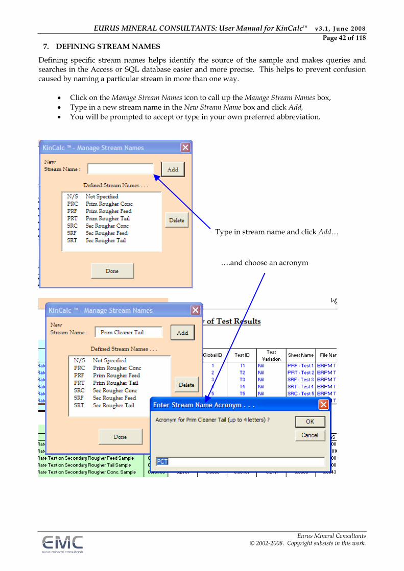
Defining specific stream names helps identify the source of the sample and makes queries and searches in the Access or SQL database easier and more precise. This helps to prevent confusion caused by naming a particular stream in more than one way.
Click on the Manage Stream Names icon to call up the Manage Stream Names box, Type in a new stream name in the New Stream Name box and click Add, You will be prompted to accept or type in your own preferred abbreviation.
Type in stream name and click Add…
….and choose an acronym
EURUS MINERAL CONSULTANTS: User Manual for KinCalc™ v3.1 , June 2008 Page 43 of 118
Eurus Mineral Consultants © 2002-2008. Copyright subsists in this work.
8. DEFINING OTHER TEST PARAMETERS
Functions available:
1. Define any test condition, sample details or any other parameter that is required to fully describe the test
2. Select preferred units of measurement 3. Order the parameters as desired
Diagrams highlighting various points detailed below can be found towards the end of this section. “Other Test Parameters” covers anything of importance other than the specific items on the Input Page. Any test and/or sample description such as reagent type and addition, grind, sample depth, sample condition or geographic location can be specified. It is best to be as detailed and specific as possible because this will be helpful when queries and searches are done in the Access or SQL database to retrieve information.
8.1. Managing Other Test Parameters
Click the Manage the List of Other Parameters icon to access the Manage Analytes and Minerals box. Any parameter can be chosen and moved to the Selected box by double clicking on it. The order in the Selected box may be changed by highlighting any parameter and clicking on the up or down arrow. A new parameter may be inserted in the Available box by clicking on Define New. Name the parameter and choose the number of decimal places required when the parameter is displayed. In the diagram below, note that a parameter of “Long description” is included. It is recommended that one or possibly two general parameters are included so that important notes can be recorded such as;
A report or folder name where hard copy notes concerning the test may be found, General conditions of the pilot plant run or plant audit that prevailed at the time, Comments on sample representivity, Notes on froth condition or other notes of a general nature concerning the test.
Note that once a parameter is loaded and used it cannot be deleted at a later date because it will have been loaded into the Database and will now be an integral part of the data management system. It is always wise to add spare columns, in this case labelled “Comments1” and “Comments 2”, to accommodate any test details or notes/comments that were either not available at the time of data input or which become available as a result of measurements performed later.
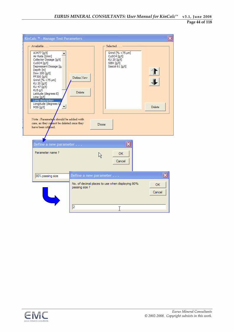
EURUS MINERAL CONSULTANTS: User Manual for KinCalc™ v3.1 , June 2008 Page 44 of 118
Eurus Mineral Consultants © 2002-2008. Copyright subsists in this work.
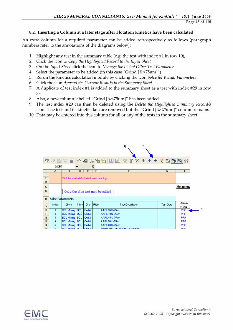
EURUS MINERAL CONSULTANTS: User Manual for KinCalc™ v3.1 , June 2008 Page 45 of 118
Eurus Mineral Consultants © 2002-2008. Copyright subsists in this work.
8.2. Inserting a Column at a later stage after Flotation Kinetics have been calculated
An extra column for a required parameter can be added retrospectively as follows (paragraph numbers refer to the annotations of the diagrams below);
1. Highlight any test in the summary table (e.g. the test with index #1 in row 10), 2. Click the icon to Copy the Highlighted Record to the Input Sheet 3. On the Input Sheet click the icon to Manage the List of Other Test Parameters 4. Select the parameter to be added (in this case “Grind [%<75um]”) 5. Rerun the kinetics calculation module by clicking the icon Solve for Kelsall Parameters 6. Click the icon Append the Current Results to the Summary Sheet 7. A duplicate of test index #1 is added to the summary sheet as a test with index #29 in row
38 8. Also, a new column labelled “Grind [%<75um]” has been added 9. The test index #29 can then be deleted using the Delete the Highlighted Summary Record/s
icon. The test and its kinetic data are removed but the “Grind [%<75um]” column remains 10. Data may be entered into this column for all or any of the tests in the summary sheet
2
1
9
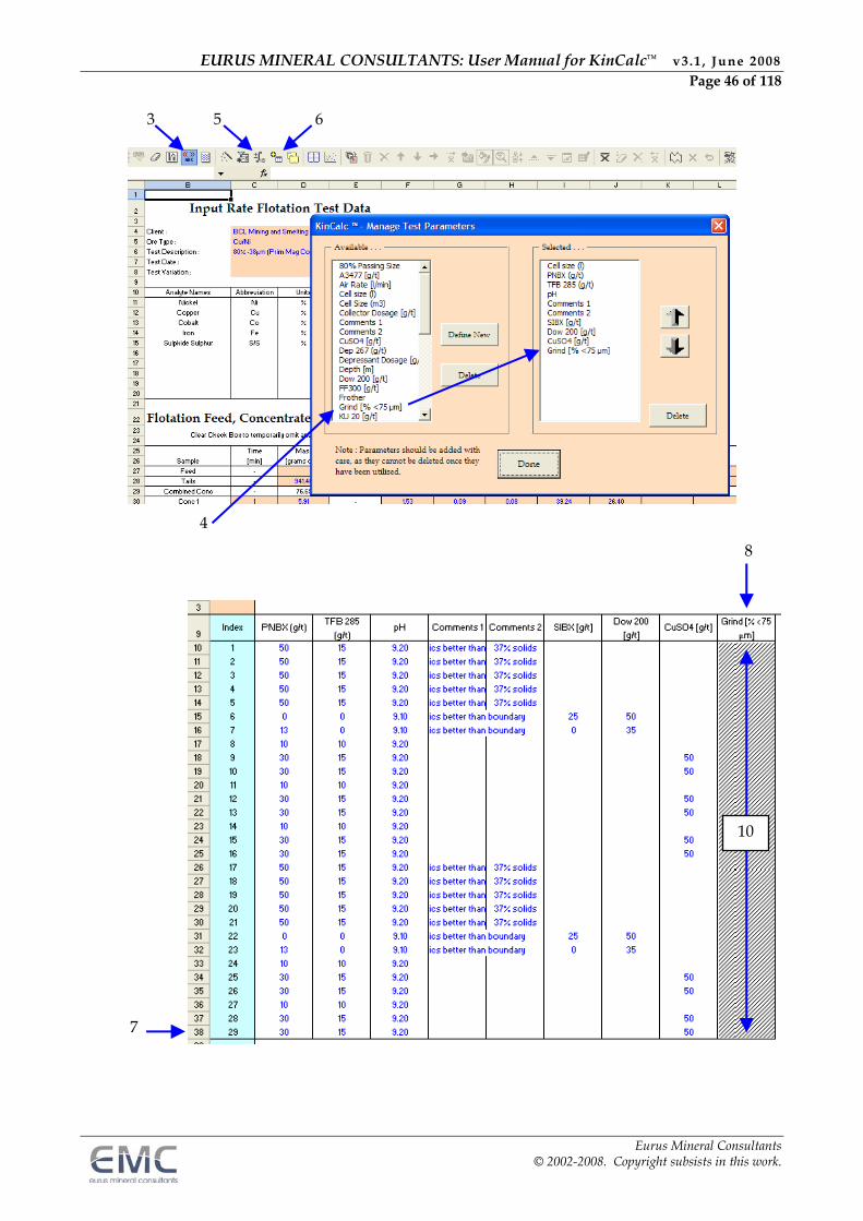
EURUS MINERAL CONSULTANTS: User Manual for KinCalc™ v3.1 , June 2008 Page 46 of 118
Eurus Mineral Consultants © 2002-2008. Copyright subsists in this work.
4
3 6 5
7
8
10
EURUS MINERAL CONSULTANTS: User Manual for KinCalc™ v3.1 , June 2008 Page 47 of 118
Eurus Mineral Consultants © 2002-2008. Copyright subsists in this work.
9. MANUAL INPUT OF TEST DATA
Functions available:
1. Input of raw data by hand or by copy/paste function 2. Input of test descriptions and conditions by hand or by copy/paste function 3. Input of other test parameters by hand 4. Screening of raw data via the Auto Report to identify data import errors before processing
Diagrams highlighting various points detailed below can be found towards the end of this section.
9.1. Manual Input of Test Data
Call up the Manage the List of Analytes and Minerals form, Select analytes and/or minerals in the required order from the Available box or
choose from the Saved Sets list and click on the Use button, This automatically loads analytes and assays onto the Input Page.
Areas where text and data may be entered are coloured Tan and anything written or pasted into these areas is formatted in blue. Areas which are not coloured are protected and no data or text can be inserted.
Go to the Input Page, Either type in or paste test data and descriptions into the respective cells, In the Stream Name cell a drop-down box appears. These are abbreviations to record
the name of the stream from which the sample was taken. If it is necessary to add a stream name do so as per section 7,
Change assay units and number of decimal places (from 2 to 4 and vice versa) as desired as per section 6.6.
The diagram below shows a typical Input page.
9.2. Manual Input of Other Test Parameters
Call up the Manage the List of other Test Parameters form, Select other parameters as described in section 8.1 above, The parameters are automatically loaded into an Other Test Parameters box at the
bottom of the Input page. The diagram below shows the bottom of a typical Input page with the list of Other Parameters as chosen from the Manage the List of other Test Parameters form.
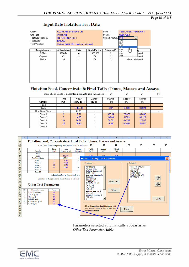
EURUS MINERAL CONSULTANTS: User Manual for KinCalc™ v3.1 , June 2008 Page 48 of 118
Eurus Mineral Consultants © 2002-2008. Copyright subsists in this work.
Parameters selected automatically appear as an Other Test Parameters table
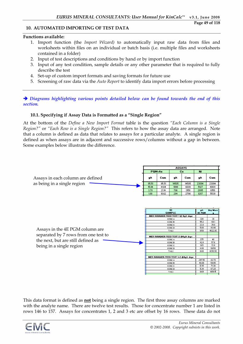
EURUS MINERAL CONSULTANTS: User Manual for KinCalc™ v3.1 , June 2008 Page 49 of 118
Eurus Mineral Consultants © 2002-2008. Copyright subsists in this work.
10. AUTOMATED IMPORTING OF TEST DATA
Functions available: 1. Import function (the Import Wizard) to automatically input raw data from files and
worksheets within files on an individual or batch basis (i.e. multiple files and worksheets contained in a folder)
2. Input of test descriptions and conditions by hand or by import function 3. Input of any test condition, sample details or any other parameter that is required to fully
describe the test 4. Set-up of custom import formats and saving formats for future use 5. Screening of raw data via the Auto Report to identify data import errors before processing
Diagrams highlighting various points detailed below can be found towards the end of this section.
10.1. Specifying if Assay Data is Formatted as a “Single Region”
At the bottom of the Define a New Import Format table is the question “Each Column is a Single Region?” or “Each Row is a Single Region?” This refers to how the assay data are arranged. Note that a column is defined as data that relates to assays for a particular analyte. A single region is defined as when assays are in adjacent and successive rows/columns without a gap in between. Some examples below illustrate the difference.
This data format is defined as not being a single region. The first three assay columns are marked with the analyte name. There are twelve test results. Those for concentrate number 1 are listed in rows 146 to 157. Assays for concentrates 1, 2 and 3 etc are offset by 16 rows. These data do not
Assays in each column are defined as being in a single region
Assays in the 4E PGM column are separated by 7 rows from one test to the next, but are still defined as being in a single region
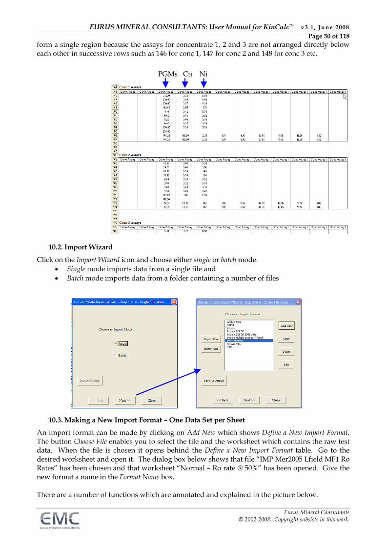
EURUS MINERAL CONSULTANTS: User Manual for KinCalc™ v3.1 , June 2008 Page 50 of 118
Eurus Mineral Consultants © 2002-2008. Copyright subsists in this work.
form a single region because the assays for concentrate 1, 2 and 3 are not arranged directly below each other in successive rows such as 146 for conc 1, 147 for conc 2 and 148 for conc 3 etc.
10.2. Import Wizard
Click on the Import Wizard icon and choose either single or batch mode. Single mode imports data from a single file and Batch mode imports data from a folder containing a number of files
10.3. Making a New Import Format – One Data Set per Sheet
An import format can be made by clicking on Add New which shows Define a New Import Format. The button Choose File enables you to select the file and the worksheet which contains the raw test data. When the file is chosen it opens behind the Define a New Import Format table. Go to the desired worksheet and open it. The dialog box below shows that file “IMP Mer2005 Lfield MF1 Ro Rates” has been chosen and that worksheet “Normal – Ro rate @ 50%” has been opened. Give the new format a name in the Format Name box.
There are a number of functions which are annotated and explained in the picture below.
PGMs Cu Ni
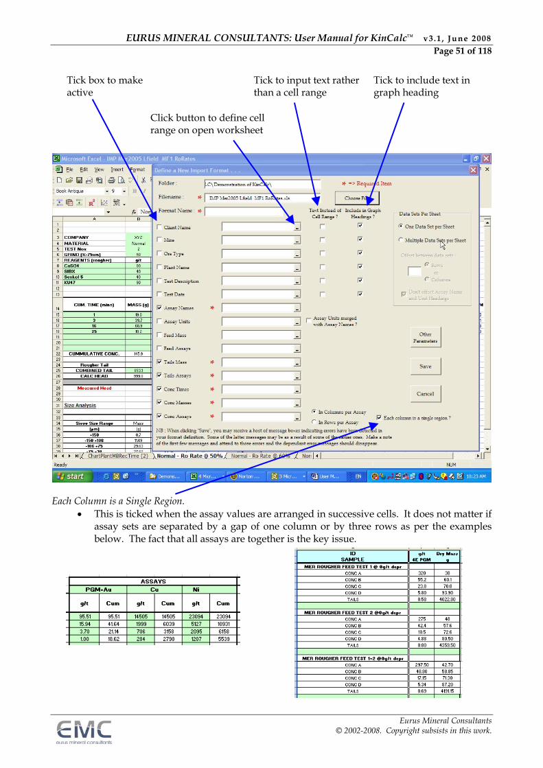
EURUS MINERAL CONSULTANTS: User Manual for KinCalc™ v3.1 , June 2008 Page 51 of 118
Eurus Mineral Consultants © 2002-2008. Copyright subsists in this work.
Each Column is a Single Region. This is ticked when the assay values are arranged in successive cells. It does not matter if
assay sets are separated by a gap of one column or by three rows as per the examples below. The fact that all assays are together is the key issue.
Tick box to make active
Tick to input text rather than a cell range
Tick to include text in graph heading
Click button to define cell range on open worksheet
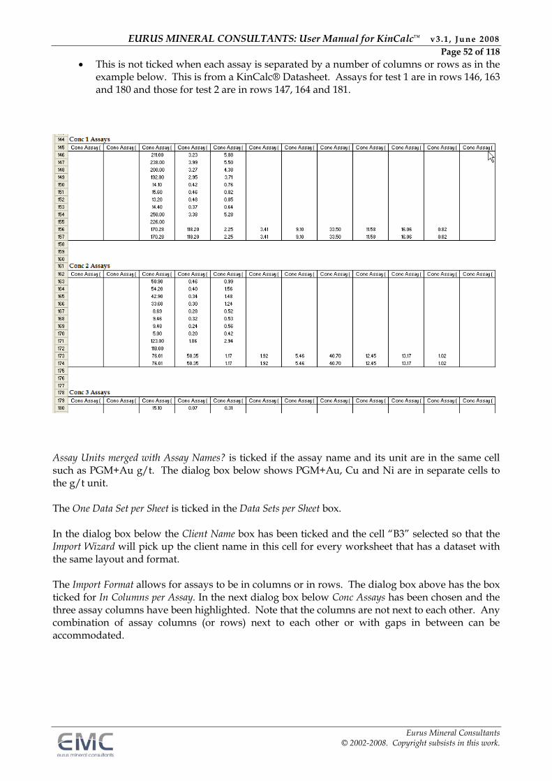
EURUS MINERAL CONSULTANTS: User Manual for KinCalc™ v3.1 , June 2008 Page 52 of 118
Eurus Mineral Consultants © 2002-2008. Copyright subsists in this work.
This is not ticked when each assay is separated by a number of columns or rows as in the example below. This is from a KinCalc® Datasheet. Assays for test 1 are in rows 146, 163 and 180 and those for test 2 are in rows 147, 164 and 181.
Assay Units merged with Assay Names? is ticked if the assay name and its unit are in the same cell such as PGM+Au g/t. The dialog box below shows PGM+Au, Cu and Ni are in separate cells to the g/t unit. The One Data Set per Sheet is ticked in the Data Sets per Sheet box. In the dialog box below the Client Name box has been ticked and the cell “B3” selected so that the Import Wizard will pick up the client name in this cell for every worksheet that has a dataset with the same layout and format. The Import Format allows for assays to be in columns or in rows. The dialog box above has the box ticked for In Columns per Assay. In the next dialog box below Conc Assays has been chosen and the three assay columns have been highlighted. Note that the columns are not next to each other. Any combination of assay columns (or rows) next to each other or with gaps in between can be accommodated.
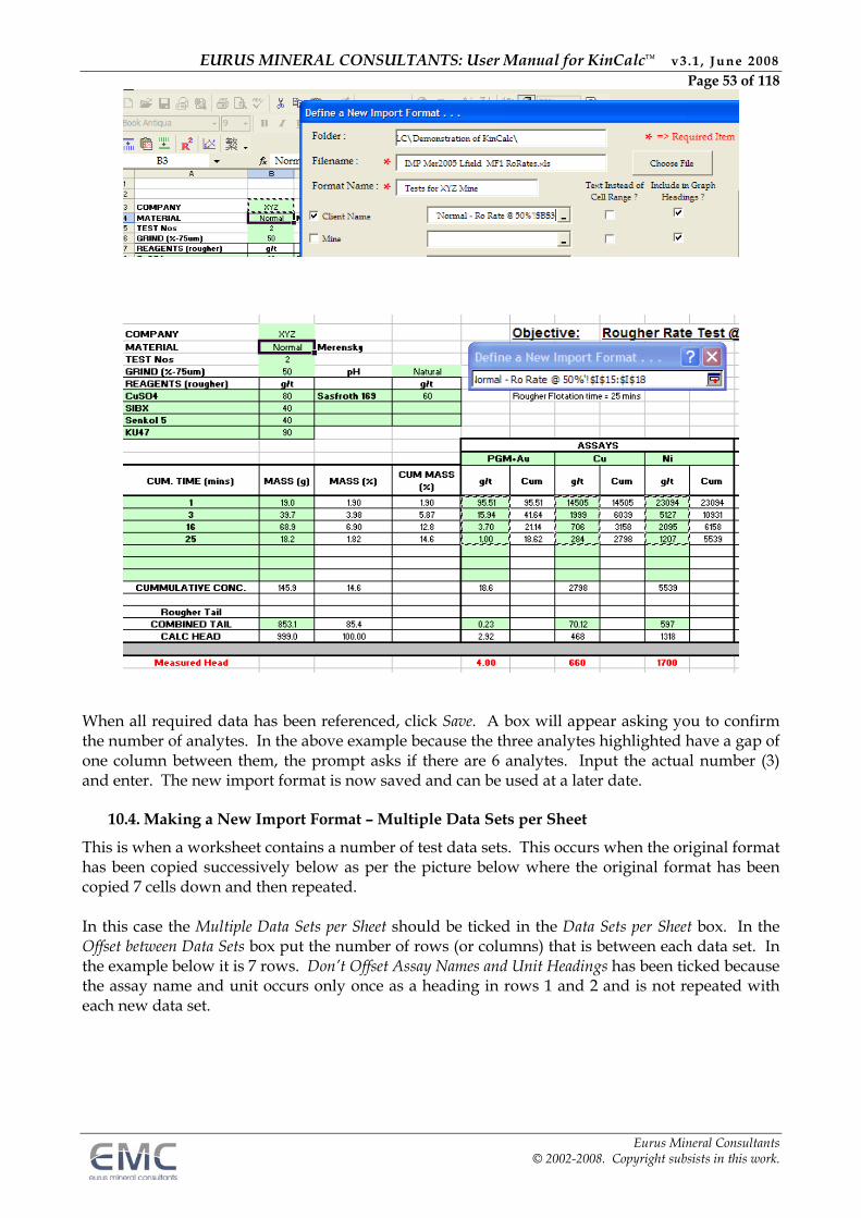
EURUS MINERAL CONSULTANTS: User Manual for KinCalc™ v3.1 , June 2008 Page 53 of 118
Eurus Mineral Consultants © 2002-2008. Copyright subsists in this work.
When all required data has been referenced, click Save. A box will appear asking you to confirm the number of analytes. In the above example because the three analytes highlighted have a gap of one column between them, the prompt asks if there are 6 analytes. Input the actual number (3) and enter. The new import format is now saved and can be used at a later date.
10.4. Making a New Import Format – Multiple Data Sets per Sheet
This is when a worksheet contains a number of test data sets. This occurs when the original format has been copied successively below as per the picture below where the original format has been copied 7 cells down and then repeated. In this case the Multiple Data Sets per Sheet should be ticked in the Data Sets per Sheet box. In the Offset between Data Sets box put the number of rows (or columns) that is between each data set. In the example below it is 7 rows. Don’t Offset Assay Names and Unit Headings has been ticked because the assay name and unit occurs only once as a heading in rows 1 and 2 and is not repeated with each new data set.
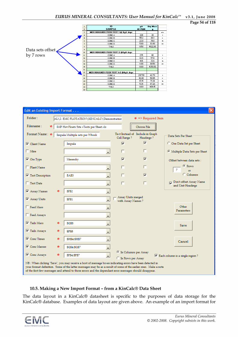
EURUS MINERAL CONSULTANTS: User Manual for KinCalc™ v3.1 , June 2008 Page 54 of 118
Eurus Mineral Consultants © 2002-2008. Copyright subsists in this work.
10.5. Making a New Import Format – from a KinCalc® Data Sheet
The data layout in a KinCalc® datasheet is specific to the purposes of data storage for the KinCalc® database. Examples of data layout are given above. An example of an import format for
Data sets offset by 7 rows
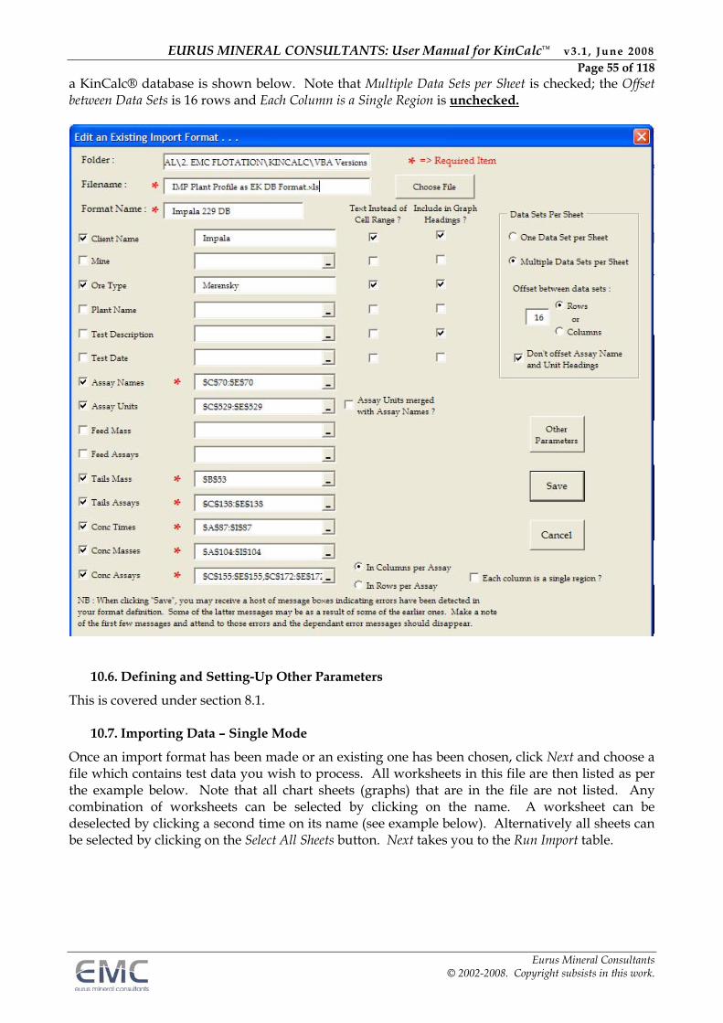
EURUS MINERAL CONSULTANTS: User Manual for KinCalc™ v3.1 , June 2008 Page 55 of 118
Eurus Mineral Consultants © 2002-2008. Copyright subsists in this work.
a KinCalc® database is shown below. Note that Multiple Data Sets per Sheet is checked; the Offset between Data Sets is 16 rows and Each Column is a Single Region is unchecked.
10.6. Defining and Setting-Up Other Parameters
This is covered under section 8.1.
10.7. Importing Data – Single Mode
Once an import format has been made or an existing one has been chosen, click Next and choose a file which contains test data you wish to process. All worksheets in this file are then listed as per the example below. Note that all chart sheets (graphs) that are in the file are not listed. Any combination of worksheets can be selected by clicking on the name. A worksheet can be deselected by clicking a second time on its name (see example below). Alternatively all sheets can be selected by clicking on the Select All Sheets button. Next takes you to the Run Import table.
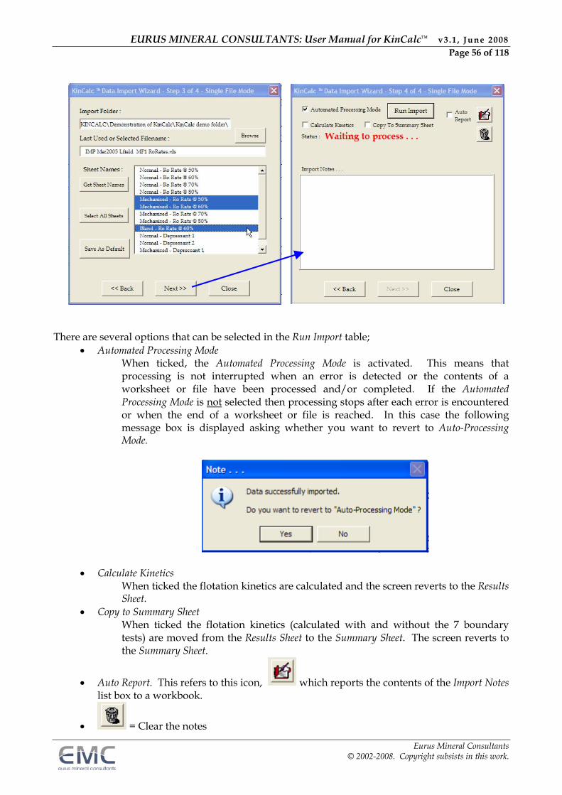
EURUS MINERAL CONSULTANTS: User Manual for KinCalc™ v3.1 , June 2008 Page 56 of 118
Eurus Mineral Consultants © 2002-2008. Copyright subsists in this work.
There are several options that can be selected in the Run Import table;
Automated Processing Mode When ticked, the Automated Processing Mode is activated. This means that processing is not interrupted when an error is detected or the contents of a worksheet or file have been processed and/or completed. If the Automated Processing Mode is not selected then processing stops after each error is encountered or when the end of a worksheet or file is reached. In this case the following message box is displayed asking whether you want to revert to Auto-Processing Mode.
Calculate Kinetics When ticked the flotation kinetics are calculated and the screen reverts to the Results Sheet.
Copy to Summary Sheet When ticked the flotation kinetics (calculated with and without the 7 boundary tests) are moved from the Results Sheet to the Summary Sheet. The screen reverts to the Summary Sheet.
Auto Report. This refers to this icon, which reports the contents of the Import Notes list box to a workbook.
= Clear the notes
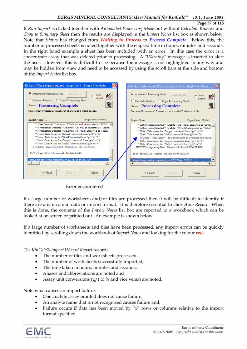
EURUS MINERAL CONSULTANTS: User Manual for KinCalc™ v3.1 , June 2008 Page 57 of 118
Eurus Mineral Consultants © 2002-2008. Copyright subsists in this work.
If Run Import is clicked together with Automated Processing Mode but without Calculate Kinetics and Copy to Summary Sheet then the results are displayed in the Import Notes list box as shown below. Note that Status has changed from Waiting to Process to Process Complete. Below this, the number of processed sheets is noted together with the elapsed time in hours, minutes and seconds. In the right hand example a sheet has been included with an error. In this case the error is a concentrate assay that was deleted prior to processing. A “Warning” message is inserted to alert the user. However this is difficult to see because the message is not highlighted in any way and may be hidden from view and need to be accessed by using the scroll bars at the side and bottom of the Import Notes list box.
If a large number of worksheets and/or files are processed then it will be difficult to identify if there are any errors in data or import format. It is therefore essential to click Auto Report. When this is done, the contents of the Import Notes list box are reported to a workbook which can be looked at on screen or printed out. An example is shown below. If a large number of worksheets and files have been processed, any import errors can be quickly identified by scrolling down the workbook of Import Notes and looking for the colour red.
The KinCalc® Import Wizard Report records:
The number of files and worksheets processed, The number of worksheets successfully imported, The time taken in hours, minutes and seconds, Aliases and abbreviations are noted and Assay unit conversions (g/t to % and vice versa) are noted.
Note what causes an import failure:
One analyte assay omitted does not cause failure, An analyte name that is not recognised causes failure and, Failure occurs if data has been moved by “x” rows or columns relative to the import
format specified.
Error encountered
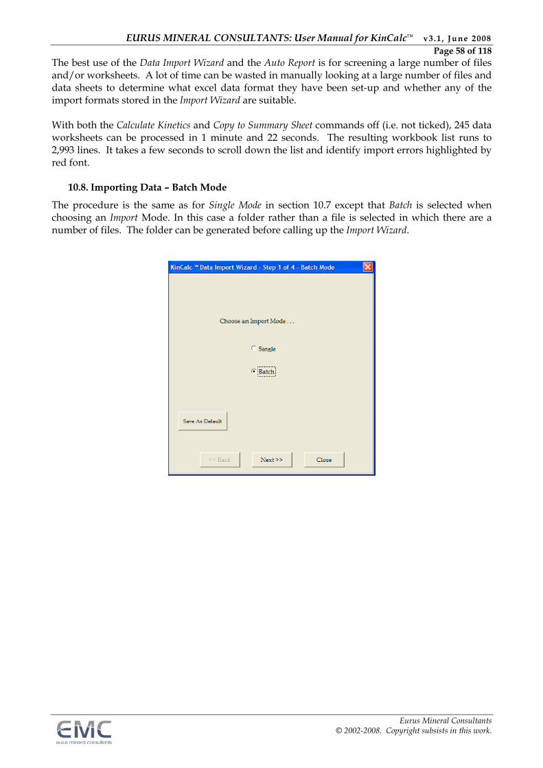
EURUS MINERAL CONSULTANTS: User Manual for KinCalc™ v3.1 , June 2008 Page 58 of 118
Eurus Mineral Consultants © 2002-2008. Copyright subsists in this work.
The best use of the Data Import Wizard and the Auto Report is for screening a large number of files and/or worksheets. A lot of time can be wasted in manually looking at a large number of files and data sheets to determine what excel data format they have been set-up and whether any of the import formats stored in the Import Wizard are suitable. With both the Calculate Kinetics and Copy to Summary Sheet commands off (i.e. not ticked), 245 data worksheets can be processed in 1 minute and 22 seconds. The resulting workbook list runs to 2,993 lines. It takes a few seconds to scroll down the list and identify import errors highlighted by red font.
10.8. Importing Data – Batch Mode
The procedure is the same as for Single Mode in section 10.7 except that Batch is selected when choosing an Import Mode. In this case a folder rather than a file is selected in which there are a number of files. The folder can be generated before calling up the Import Wizard.
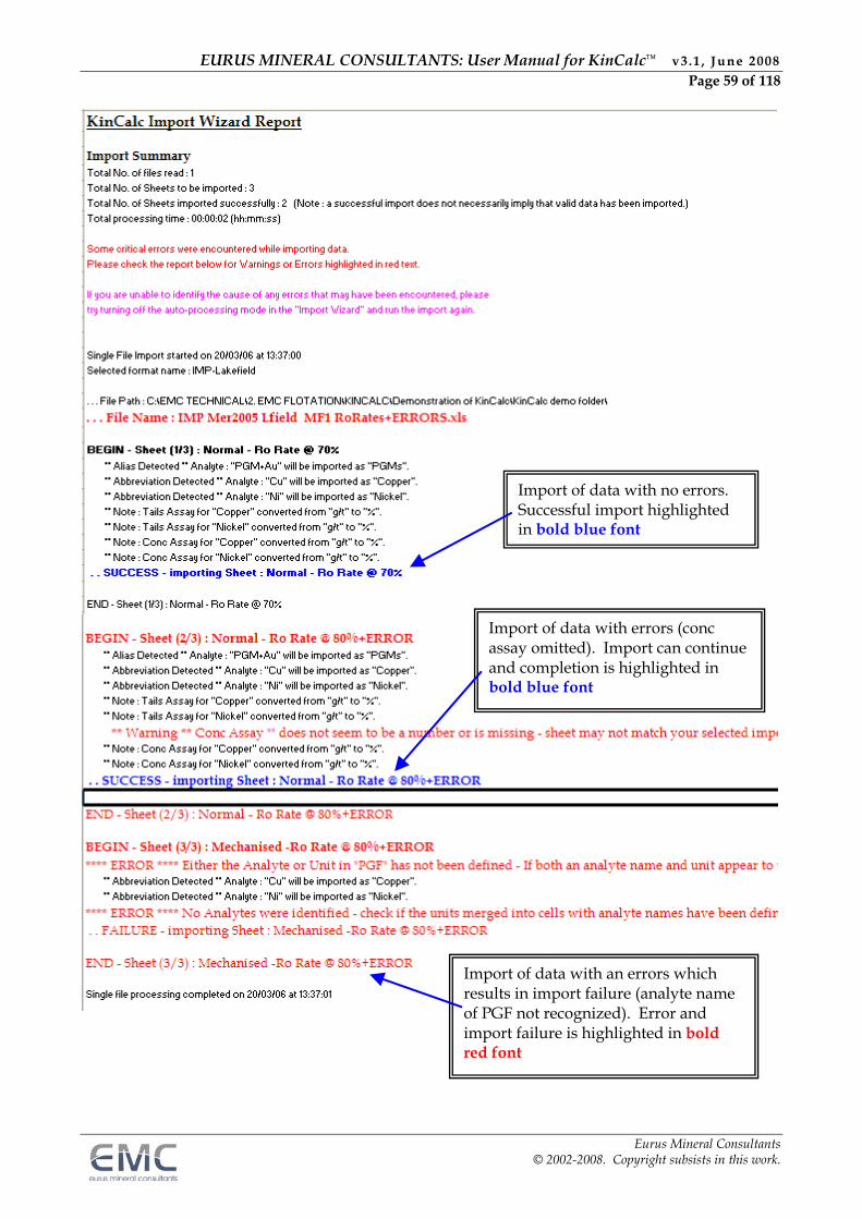
EURUS MINERAL CONSULTANTS: User Manual for KinCalc™ v3.1 , June 2008 Page 59 of 118
Eurus Mineral Consultants © 2002-2008. Copyright subsists in this work.
Import of data with no errors. Successful import highlighted in bold blue font
Import of data with errors (conc assay omitted). Import can continue and completion is highlighted in bold blue font
Import of data with an errors which results in import failure (analyte name of PGF not recognized). Error and import failure is highlighted in bold red font
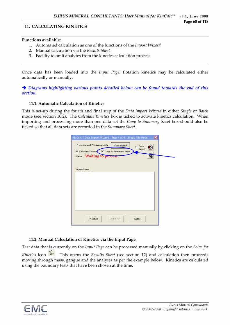
EURUS MINERAL CONSULTANTS: User Manual for KinCalc™ v3.1 , June 2008 Page 60 of 118
Eurus Mineral Consultants © 2002-2008. Copyright subsists in this work.
11. CALCULATING KINETICS
Functions available:
1. Automated calculation as one of the functions of the Import Wizard 2. Manual calculation via the Results Sheet 3. Facility to omit analytes from the kinetics calculation process
Once data has been loaded into the Input Page, flotation kinetics may be calculated either automatically or manually. Diagrams highlighting various points detailed below can be found towards the end of this section.
11.1. Automatic Calculation of Kinetics
This is set-up during the fourth and final step of the Data Import Wizard in either Single or Batch mode (see section 10.2). The Calculate Kinetics box is ticked to activate kinetics calculation. When importing and processing more than one data set the Copy to Summary Sheet box should also be ticked so that all data sets are recorded in the Summary Sheet.
11.2. Manual Calculation of Kinetics via the Input Page
Test data that is currently on the Input Page can be processed manually by clicking on the Solve for
Kinetics icon . This opens the Results Sheet (see section 12) and calculation then proceeds moving through mass, gangue and the analytes as per the example below. Kinetics are calculated using the boundary tests that have been chosen at the time.
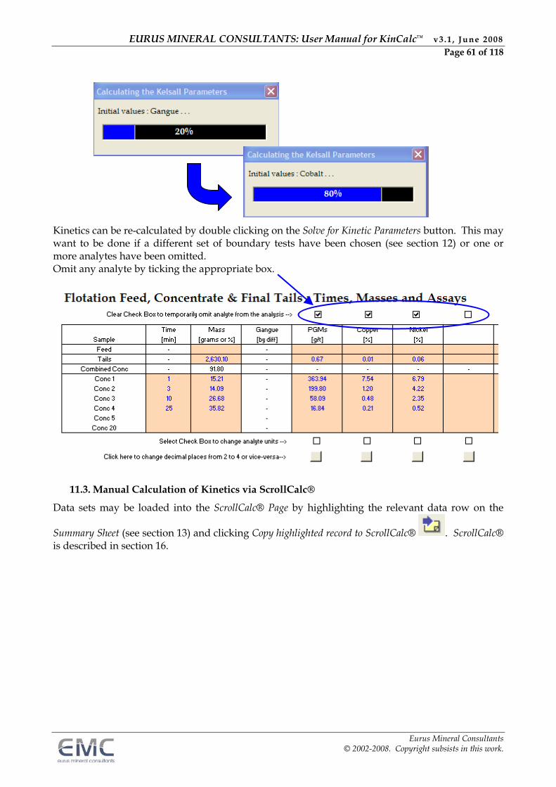
EURUS MINERAL CONSULTANTS: User Manual for KinCalc™ v3.1 , June 2008 Page 61 of 118
Eurus Mineral Consultants © 2002-2008. Copyright subsists in this work.
Kinetics can be re-calculated by double clicking on the Solve for Kinetic Parameters button. This may want to be done if a different set of boundary tests have been chosen (see section 12) or one or more analytes have been omitted. Omit any analyte by ticking the appropriate box.
11.3. Manual Calculation of Kinetics via ScrollCalc®
Data sets may be loaded into the ScrollCalc® Page by highlighting the relevant data row on the
Summary Sheet (see section 13) and clicking Copy highlighted record to ScrollCalc® . ScrollCalc® is described in section 16.
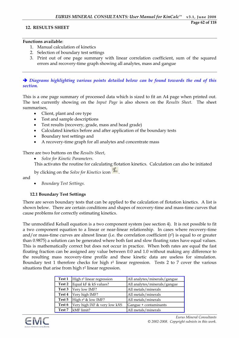
EURUS MINERAL CONSULTANTS: User Manual for KinCalc™ v3.1 , June 2008 Page 62 of 118
Eurus Mineral Consultants © 2002-2008. Copyright subsists in this work.
12. RESULTS SHEET
Functions available:
1. Manual calculation of kinetics 2. Selection of boundary test settings 3. Print out of one page summary with linear correlation coefficient, sum of the squared
errors and recovery-time graph showing all analytes, mass and gangue Diagrams highlighting various points detailed below can be found towards the end of this section. This is a one page summary of processed data which is sized to fit an A4 page when printed out. The test currently showing on the Input Page is also shown on the Results Sheet. The sheet summarises,
Client, plant and ore type Test and sample descriptions Test results (recovery, grade, mass and head grade) Calculated kinetics before and after application of the boundary tests Boundary test settings and A recovery-time graph for all analytes and concentrate mass
There are two buttons on the Results Sheet,
Solve for Kinetic Parameters. This activates the routine for calculating flotation kinetics. Calculation can also be initiated
by clicking on the Solve for Kinetics icon . and
Boundary Test Settings.
12.1 Boundary Test Settings
There are seven boundary tests that can be applied to the calculation of flotation kinetics. A list is shown below. There are certain conditions and shapes of recovery-time and mass-time curves that cause problems for correctly estimating kinetics. The unmodified Kelsall equation is a two component system (see section 4). It is not possible to fit a two component equation to a linear or near-linear relationship. In cases where recovery-time and/or mass-time curves are almost linear (i.e. the correlation coefficient (r2) is equal to or greater than 0.9875) a solution can be generated where both fast and slow floating rates have equal values. This is mathematically correct but does not occur in practice. When both rates are equal the fast floating fraction can be assigned any value between 0.0 and 1.0 without making any difference to the resulting mass recovery-time profile and these kinetic data are useless for simulation. Boundary test 1 therefore checks for high r2 linear regression. Tests 2 to 7 cover the various situations that arise from high r2 linear regression.
Test 1 High r² linear regression All analytes/minerals/gangueTest 2 Equal kF & kS values? All analytes/minerals/gangueTest 3 Very low IMF? All metals/mineralsTest 4 Very high IMF? All metals/mineralsTest 5 High r² & low IMF? All metals/mineralsTest 6 Very high IXF & very low kXS Gangue + contaminantsTest 7 kMF limit? All metals/minerals
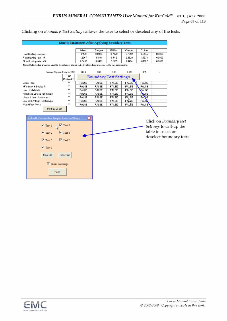
EURUS MINERAL CONSULTANTS: User Manual for KinCalc™ v3.1 , June 2008 Page 63 of 118
Eurus Mineral Consultants © 2002-2008. Copyright subsists in this work.
Click on Boundary test Settings to call-up the table to select or deselect boundary tests.
Clicking on Boundary Test Settings allows the user to select or deselect any of the tests.
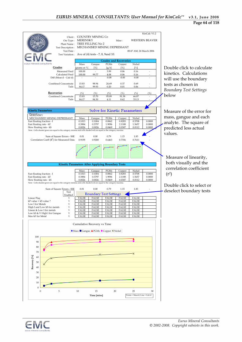
EURUS MINERAL CONSULTANTS: User Manual for KinCalc™ v3.1 , June 2008 Page 64 of 118
Eurus Mineral Consultants © 2002-2008. Copyright subsists in this work.
KinCalc V1.2 Client : COUNTRY MINING Co
Ore Type : MERENSKY Mine : WESTERN BEAVERPlant Name : TREE FELLING No 2
Test Description : MECHANISED MINING DEPRESSANTTest Date : 08:47 AM; 24 March 2006
Test Variation : Ave of (4) tests - 7, 8, 9and 10.
Grades and RecoveriesMass Gangue PGMs Copper Nickel
Grades [grams or %] [%] [g/t] [%] [%]
Measured Feed 100.00 - 3.99 0.06 0.16 -Calculated Feed 100.00 99.77 4.08 0.06 0.16 -
Diff (Meas'd - Calc'd) - - -0.08 -0.00 -0.00 -
Combined Concentrate 15.83 98.94 24.69 0.37 0.69 -Tails 84.17 99.93 0.20 0.01 0.06 -
Recoveries (%) (%) (%) (%) (%) (%)Combined Concentrate 15.83 15.70 95.89 91.38 66.87 -
Tails 84.17 84.30 4.11 8.62 33.13 -
Kinetic Parameters MERENSKY MECHANISED MINING DEPRESSANT Mass Gangue PGMs Copper NickelFast floating fraction - I 0.1013 0.1004 0.8862 0.8283 0.5708 0.0000Fast floating rate - kF 0.3884 0.3797 1.9096 2.1188 1.5657 0.0000Slow floating rate - kS 0.0026 0.0026 0.0469 0.0307 0.0112 0.0000
Sum of Square Errors - SSE 0.01 0.00 0.79 1.15 1.83 -Correlation Coeff (R2) for Measured Data 0.9195 0.9200 0.6463 0.7356 0.7611 -
Kinetic Parameters After Applying Boundary Tests
Mass Gangue PGMs Copper NickelFast floating fraction - I 0.1013 0.1004 0.8862 0.8283 0.5708 0.0000Fast floating rate - kF 0.3884 0.3797 1.9096 2.1188 1.5657 0.0000Slow floating rate - kS 0.0026 0.0026 0.0469 0.0307 0.0112 0.0000
Sum of Square Errors - SSE 0.01 0.00 0.79 1.15 1.83 -
Linear Flag Y FALSE FALSE FALSE FALSE FALSEkF value = kS value ? Y FALSE FALSE FALSE FALSE FALSELow I for Metals Y FALSE FALSE FALSE FALSE FALSEHigh I and Low kS for metals Y FALSE FALSE FALSE FALSE FALSELinear & Low I for metals Y FALSE FALSE FALSE FALSE FALSELow kS & V High I for Gangue Y FALSE FALSE FALSE FALSE FALSEMax kF for Metal Y FALSE FALSE FALSE FALSE FALSE
TestEnabled
Note : Cells shaded green are equal to the category minima and cells shaded red are equal to the category maxima.
Note : Cells shaded green are equal to the category minima and cells shaded red are equal to the category maxima.
Cumulative Recovery vs Time
0
10
20
30
40
50
60
70
80
90
100
0 5 10 15 20 25 30
Time [mins]
Rec
over
y [%
]
Mass Gangue PGMs Copper Nickel
Points = Meas'd; Line = Calc'd
Measure of the error for mass, gangue and each analyte. The square of predicted less actual values.
Measure of linearity, both visually and the correlation coefficient (r2)
Double click to select or deselect boundary tests
Double click to calculate kinetics. Calculations will use the boundary tests as chosen in Boundary Test Settings below
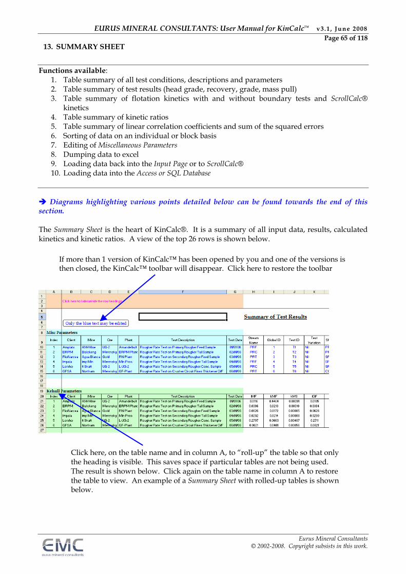
EURUS MINERAL CONSULTANTS: User Manual for KinCalc™ v3.1 , June 2008 Page 65 of 118
Eurus Mineral Consultants © 2002-2008. Copyright subsists in this work.
13. SUMMARY SHEET
Functions available:
1. Table summary of all test conditions, descriptions and parameters 2. Table summary of test results (head grade, recovery, grade, mass pull) 3. Table summary of flotation kinetics with and without boundary tests and ScrollCalc®
kinetics 4. Table summary of kinetic ratios 5. Table summary of linear correlation coefficients and sum of the squared errors 6. Sorting of data on an individual or block basis 7. Editing of Miscellaneous Parameters 8. Dumping data to excel 9. Loading data back into the Input Page or to ScrollCalc® 10. Loading data into the Access or SQL Database
Diagrams highlighting various points detailed below can be found towards the end of this section. The Summary Sheet is the heart of KinCalc®. It is a summary of all input data, results, calculated kinetics and kinetic ratios. A view of the top 26 rows is shown below.
Click here, on the table name and in column A, to “roll-up” the table so that only the heading is visible. This saves space if particular tables are not being used. The result is shown below. Click again on the table name in column A to restore the table to view. An example of a Summary Sheet with rolled-up tables is shown below.
If more than 1 version of KinCalc™ has been opened by you and one of the versions is then closed, the KinCalc™ toolbar will disappear. Click here to restore the toolbar
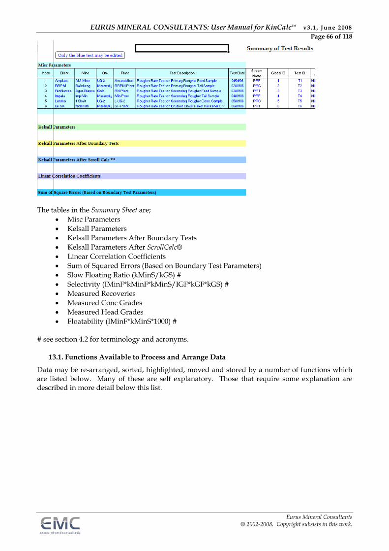
EURUS MINERAL CONSULTANTS: User Manual for KinCalc™ v3.1 , June 2008 Page 66 of 118
Eurus Mineral Consultants © 2002-2008. Copyright subsists in this work.
The tables in the Summary Sheet are;
Misc Parameters Kelsall Parameters Kelsall Parameters After Boundary Tests Kelsall Parameters After ScrollCalc® Linear Correlation Coefficients Sum of Squared Errors (Based on Boundary Test Parameters) Slow Floating Ratio (kMinS/kGS) # Selectivity (IMinF*kMinF*kMinS/IGF*kGF*kGS) # Measured Recoveries Measured Conc Grades Measured Head Grades Floatability (IMinF*kMinS*1000) #
# see section 4.2 for terminology and acronyms.
13.1. Functions Available to Process and Arrange Data
Data may be re-arranged, sorted, highlighted, moved and stored by a number of functions which are listed below. Many of these are self explanatory. Those that require some explanation are described in more detail below this list.
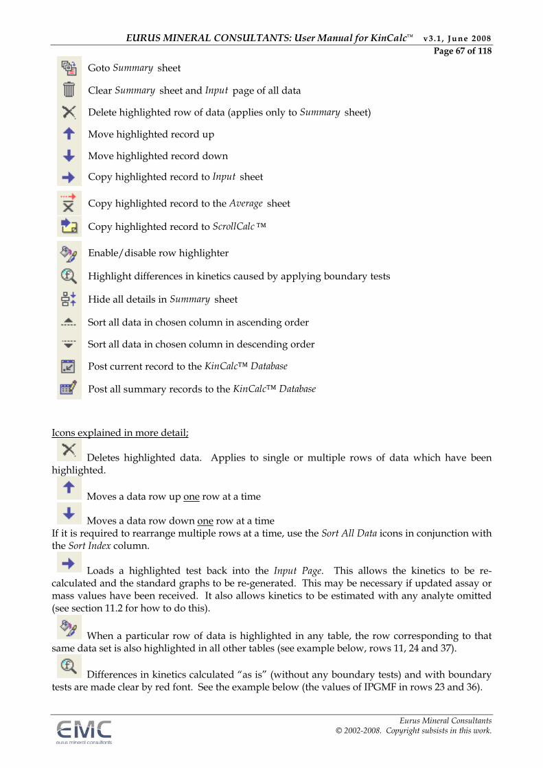
EURUS MINERAL CONSULTANTS: User Manual for KinCalc™ v3.1 , June 2008 Page 67 of 118
Eurus Mineral Consultants © 2002-2008. Copyright subsists in this work.
Goto Summary sheet
Clear Summary sheet and Input page of all data
Delete highlighted row of data (applies only to Summary sheet)
Move highlighted record up
Move highlighted record down
Copy highlighted record to Input sheet
Copy highlighted record to the Average sheet
Copy highlighted record to ScrollCalc ™
Enable/disable row highlighter
Highlight differences in kinetics caused by applying boundary tests
Hide all details in Summary sheet
Sort all data in chosen column in ascending order
Sort all data in chosen column in descending order
Post current record to the KinCalc™ Database
Post all summary records to the KinCalc™ Database
Icons explained in more detail;
Deletes highlighted data. Applies to single or multiple rows of data which have been highlighted.
Moves a data row up one row at a time
Moves a data row down one row at a time If it is required to rearrange multiple rows at a time, use the Sort All Data icons in conjunction with the Sort Index column.
Loads a highlighted test back into the Input Page. This allows the kinetics to be re-calculated and the standard graphs to be re-generated. This may be necessary if updated assay or mass values have been received. It also allows kinetics to be estimated with any analyte omitted (see section 11.2 for how to do this).
When a particular row of data is highlighted in any table, the row corresponding to that same data set is also highlighted in all other tables (see example below, rows 11, 24 and 37).
Differences in kinetics calculated “as is” (without any boundary tests) and with boundary tests are made clear by red font. See the example below (the values of IPGMF in rows 23 and 36).
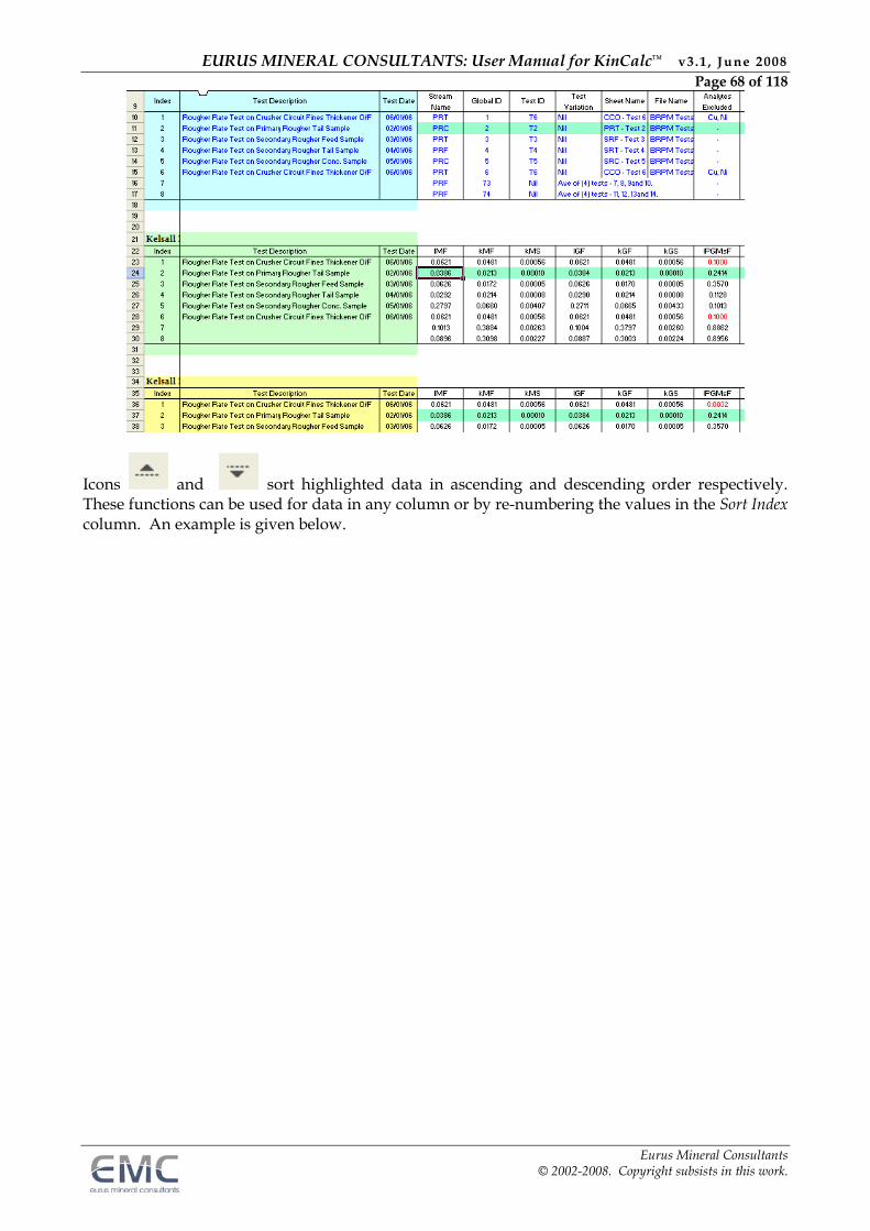
EURUS MINERAL CONSULTANTS: User Manual for KinCalc™ v3.1 , June 2008 Page 68 of 118
Eurus Mineral Consultants © 2002-2008. Copyright subsists in this work.
Icons and sort highlighted data in ascending and descending order respectively. These functions can be used for data in any column or by re-numbering the values in the Sort Index column. An example is given below.
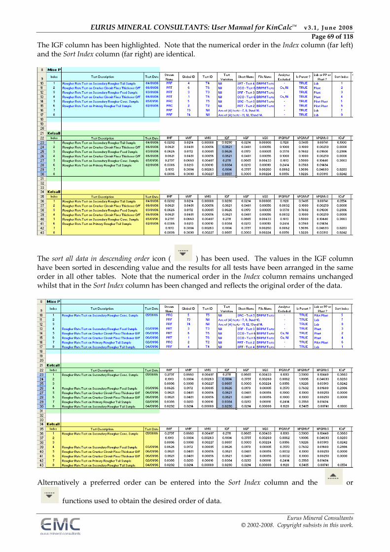
EURUS MINERAL CONSULTANTS: User Manual for KinCalc™ v3.1 , June 2008 Page 69 of 118
Eurus Mineral Consultants © 2002-2008. Copyright subsists in this work.
The IGF column has been highlighted. Note that the numerical order in the Index column (far left) and the Sort Index column (far right) are identical.
The sort all data in descending order icon ( ) has been used. The values in the IGF column have been sorted in descending value and the results for all tests have been arranged in the same order in all other tables. Note that the numerical order in the Index column remains unchanged whilst that in the Sort Index column has been changed and reflects the original order of the data.
Alternatively a preferred order can be entered into the Sort Index column and the or
functions used to obtain the desired order of data.
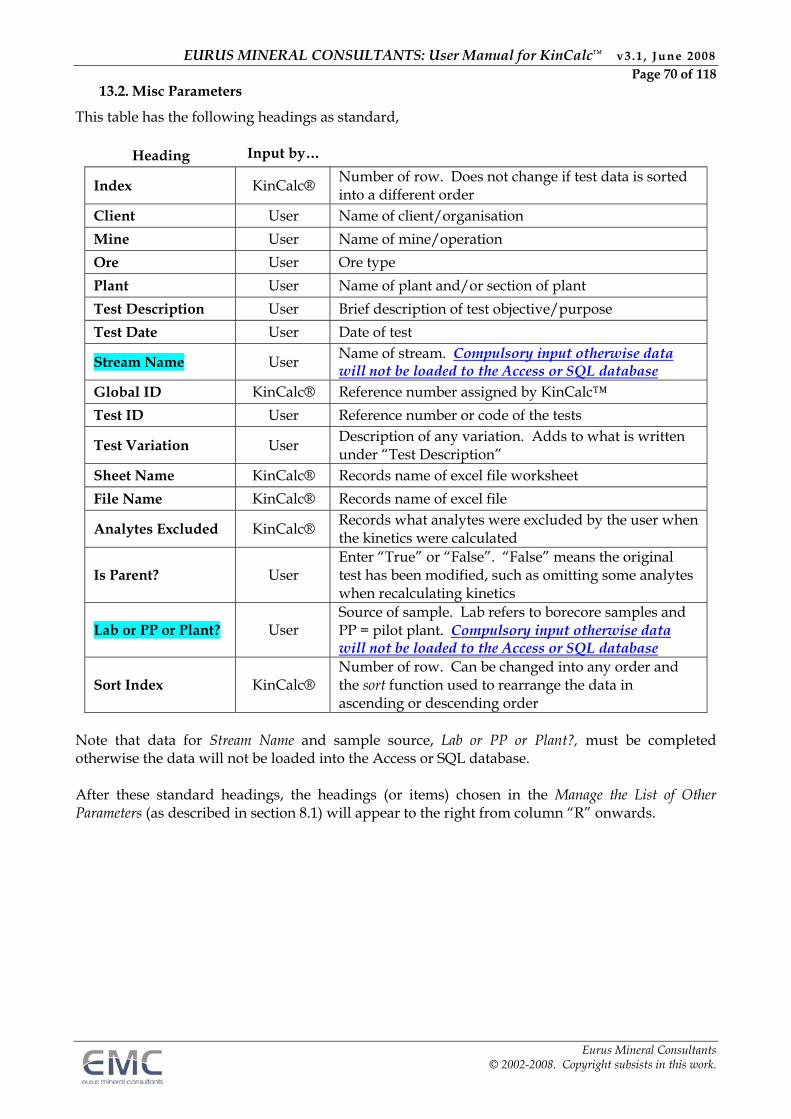
EURUS MINERAL CONSULTANTS: User Manual for KinCalc™ v3.1 , June 2008 Page 70 of 118
Eurus Mineral Consultants © 2002-2008. Copyright subsists in this work.
13.2. Misc Parameters
This table has the following headings as standard,
Heading Input by…
Index KinCalc® Number of row. Does not change if test data is sorted into a different order
Client User Name of client/organisation
Mine User Name of mine/operation
Ore User Ore type
Plant User Name of plant and/or section of plant
Test Description User Brief description of test objective/purpose
Test Date User Date of test
Stream Name User Name of stream. Compulsory input otherwise data will not be loaded to the Access or SQL database
Global ID KinCalc® Reference number assigned by KinCalc™
Test ID User Reference number or code of the tests
Test Variation User Description of any variation. Adds to what is written under “Test Description”
Sheet Name KinCalc® Records name of excel file worksheet
File Name KinCalc® Records name of excel file
Analytes Excluded KinCalc® Records what analytes were excluded by the user when the kinetics were calculated
Is Parent? User Enter “True” or “False”. “False” means the original test has been modified, such as omitting some analytes when recalculating kinetics
Lab or PP or Plant? User Source of sample. Lab refers to borecore samples and PP = pilot plant. Compulsory input otherwise data will not be loaded to the Access or SQL database
Sort Index KinCalc® Number of row. Can be changed into any order and the sort function used to rearrange the data in ascending or descending order
Note that data for Stream Name and sample source, Lab or PP or Plant?, must be completed otherwise the data will not be loaded into the Access or SQL database. After these standard headings, the headings (or items) chosen in the Manage the List of Other Parameters (as described in section 8.1) will appear to the right from column “R” onwards.
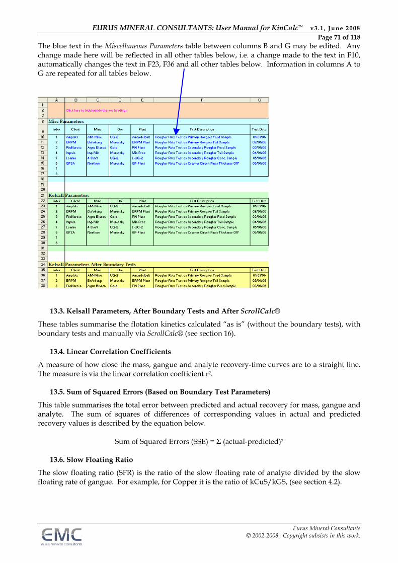
EURUS MINERAL CONSULTANTS: User Manual for KinCalc™ v3.1 , June 2008 Page 71 of 118
Eurus Mineral Consultants © 2002-2008. Copyright subsists in this work.
The blue text in the Miscellaneous Parameters table between columns B and G may be edited. Any change made here will be reflected in all other tables below, i.e. a change made to the text in F10, automatically changes the text in F23, F36 and all other tables below. Information in columns A to G are repeated for all tables below.
13.3. Kelsall Parameters, After Boundary Tests and After ScrollCalc®
These tables summarise the flotation kinetics calculated “as is” (without the boundary tests), with boundary tests and manually via ScrollCalc® (see section 16).
13.4. Linear Correlation Coefficients
A measure of how close the mass, gangue and analyte recovery-time curves are to a straight line. The measure is via the linear correlation coefficient r2.
13.5. Sum of Squared Errors (Based on Boundary Test Parameters)
This table summarises the total error between predicted and actual recovery for mass, gangue and analyte. The sum of squares of differences of corresponding values in actual and predicted recovery values is described by the equation below.
Sum of Squared Errors (SSE) = Σ (actual-predicted)2
13.6. Slow Floating Ratio
The slow floating ratio (SFR) is the ratio of the slow floating rate of analyte divided by the slow floating rate of gangue. For example, for Copper it is the ratio of kCuS/kGS, (see section 4.2).
EURUS MINERAL CONSULTANTS: User Manual for KinCalc™ v3.1 , June 2008 Page 72 of 118
Eurus Mineral Consultants © 2002-2008. Copyright subsists in this work.
13.7. Selectivity
A global measure of how one analyte floats relative to another or to floatable gangue. For Copper relative to gangue selectivity is defined by (ICuF*kCuF*kCuS)/(IGF*kGF*kGS). It is the combination of fast floating fraction, fast floating rate and slow floating rate of an analyte relative to gangue or another analyte , (see section 4.2).
13.8. Measured Recoveries and Concentrate Grades
These tables summarise the actual recoveries and concentrate grades of the tests being analysed.
13.9. Calculated Head Grades
A summary of the head grades calculated from actual mass and assay from each test.
13.10. Floatability
A measure of how well or poorly mass, gangue or an analyte floats. For Copper, floatability is described by (ICuF*kCuS*1000). It is the combination of fast floating fraction and slow floating rate as these two parameters account for the largest influence in flotation performance, (see section 4.2).
14. DATA SHEET
Functions available: 1. Stores data in a form suitable for transfer to the Access or SQL Database and the other users
of KinCalc® Diagrams highlighting various points detailed below can be found towards the end of this section.
The Data Sheet is accessed by the icon . This sheet is solely for the purpose of storing test and processed data in preparation for loading into the Access or SQL Database. No editing of data in this workbook is allowed. The following warning and comment is posted along rows 1-4 of the worksheet,
You may not edit anything on this sheet as you could compromise the integrity of data posted to the database. Note: Data reflected under the “test Info” and “Misc Parameters” below is not automatically synchronised with its source data on the Summary Sheet. If e.g. a test description is edited on the Summary Sheet, it will only be updated on this sheet if a sort operation is performed on the Summary Sheet. Data for these two headings is captured from the Summary Sheet before being posted to the Access or SQL Database. If you want to duplicate this sheet to work with the contained data, and any of the aforementioned data items has been edited on the Summary Sheet, then this sheet may be updated by performing a sort operation on the Summary sheet.
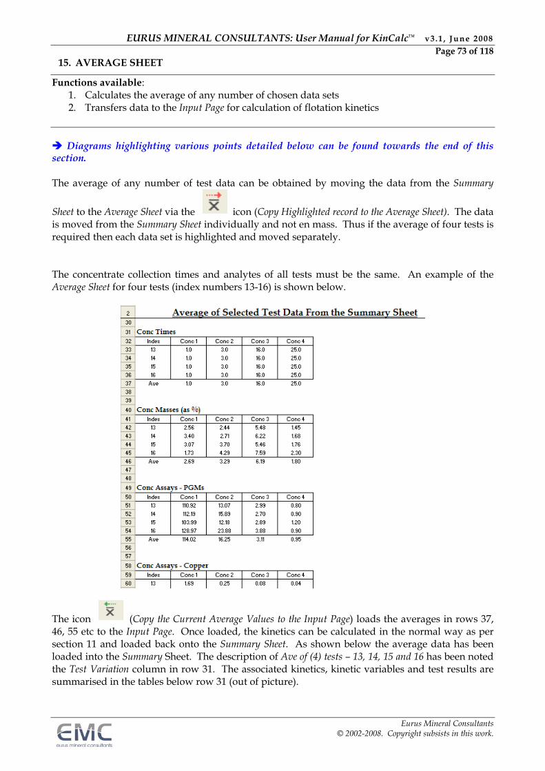
EURUS MINERAL CONSULTANTS: User Manual for KinCalc™ v3.1 , June 2008 Page 73 of 118
Eurus Mineral Consultants © 2002-2008. Copyright subsists in this work.
15. AVERAGE SHEET
Functions available: 1. Calculates the average of any number of chosen data sets 2. Transfers data to the Input Page for calculation of flotation kinetics
Diagrams highlighting various points detailed below can be found towards the end of this section. The average of any number of test data can be obtained by moving the data from the Summary
Sheet to the Average Sheet via the icon (Copy Highlighted record to the Average Sheet). The data is moved from the Summary Sheet individually and not en mass. Thus if the average of four tests is required then each data set is highlighted and moved separately. The concentrate collection times and analytes of all tests must be the same. An example of the Average Sheet for four tests (index numbers 13-16) is shown below.
The icon (Copy the Current Average Values to the Input Page) loads the averages in rows 37, 46, 55 etc to the Input Page. Once loaded, the kinetics can be calculated in the normal way as per section 11 and loaded back onto the Summary Sheet. As shown below the average data has been loaded into the Summary Sheet. The description of Ave of (4) tests – 13, 14, 15 and 16 has been noted the Test Variation column in row 31. The associated kinetics, kinetic variables and test results are summarised in the tables below row 31 (out of picture).
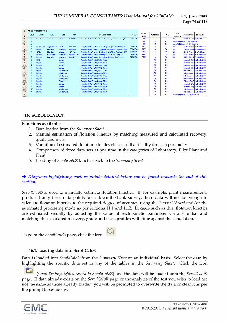
EURUS MINERAL CONSULTANTS: User Manual for KinCalc™ v3.1 , June 2008 Page 74 of 118
Eurus Mineral Consultants © 2002-2008. Copyright subsists in this work.
16. SCROLLCALC®
Functions available: 1. Data loaded from the Summary Sheet 2. Manual estimation of flotation kinetics by matching measured and calculated recovery,
grade and mass 3. Variation of estimated flotation kinetics via a scrollbar facility for each parameter 4. Comparison of three data sets at one time in the categories of Laboratory, Pilot Plant and
Plant 5. Loading of ScrollCalc® kinetics back to the Summary Sheet
Diagrams highlighting various points detailed below can be found towards the end of this section. ScrollCalc® is used to manually estimate flotation kinetics. If, for example, plant measurements produced only three data points for a down-the-bank survey, these data will not be enough to calculate flotation kinetics to the required degree of accuracy using the Import Wizard and/or the automated processing mode as per sections 11.1 and 11.2. In cases such as this, flotation kinetics are estimated visually by adjusting the value of each kinetic parameter via a scrollbar and matching the calculated recovery, grade and mass profiles with time against the actual data.
To go to the ScrollCalc® page, click the icon .
16.1. Loading data into ScrollCalc®
Data is loaded into ScrollCalc® from the Summary Sheet on an individual basis. Select the data by highlighting the specific data set in any of the tables in the Summary Sheet. Click the icon
(Copy the highlighted record to ScrollCalc®) and the data will be loaded onto the ScrollCalc® page. If data already exists on the ScrollCalc® page or the analytes of the test you wish to load are not the same as those already loaded, you will be prompted to overwrite the data or clear it as per the prompt boxes below.
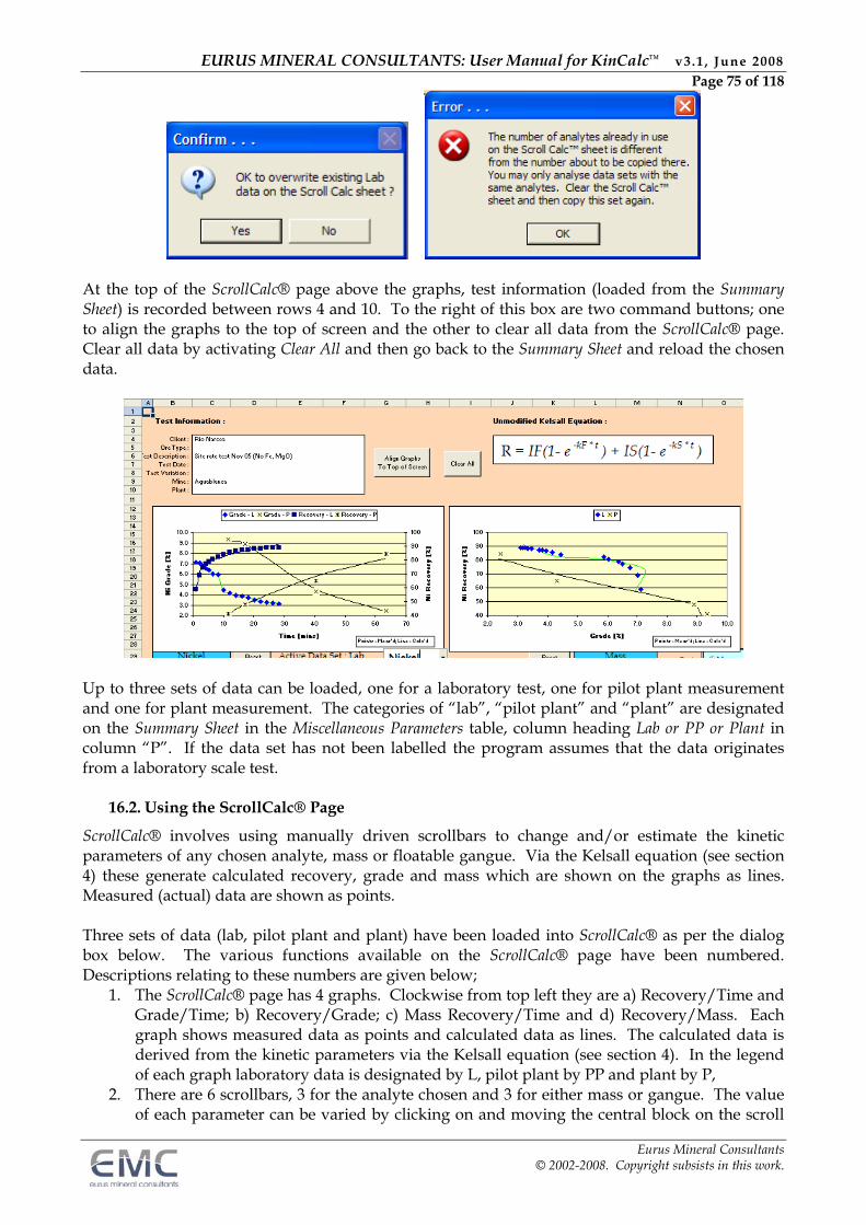
EURUS MINERAL CONSULTANTS: User Manual for KinCalc™ v3.1 , June 2008 Page 75 of 118
Eurus Mineral Consultants © 2002-2008. Copyright subsists in this work.
At the top of the ScrollCalc® page above the graphs, test information (loaded from the Summary Sheet) is recorded between rows 4 and 10. To the right of this box are two command buttons; one to align the graphs to the top of screen and the other to clear all data from the ScrollCalc® page. Clear all data by activating Clear All and then go back to the Summary Sheet and reload the chosen data.
Up to three sets of data can be loaded, one for a laboratory test, one for pilot plant measurement and one for plant measurement. The categories of “lab”, “pilot plant” and “plant” are designated on the Summary Sheet in the Miscellaneous Parameters table, column heading Lab or PP or Plant in column “P”. If the data set has not been labelled the program assumes that the data originates from a laboratory scale test.
16.2. Using the ScrollCalc® Page
ScrollCalc® involves using manually driven scrollbars to change and/or estimate the kinetic parameters of any chosen analyte, mass or floatable gangue. Via the Kelsall equation (see section 4) these generate calculated recovery, grade and mass which are shown on the graphs as lines. Measured (actual) data are shown as points. Three sets of data (lab, pilot plant and plant) have been loaded into ScrollCalc® as per the dialog box below. The various functions available on the ScrollCalc® page have been numbered. Descriptions relating to these numbers are given below;
1. The ScrollCalc® page has 4 graphs. Clockwise from top left they are a) Recovery/Time and Grade/Time; b) Recovery/Grade; c) Mass Recovery/Time and d) Recovery/Mass. Each graph shows measured data as points and calculated data as lines. The calculated data is derived from the kinetic parameters via the Kelsall equation (see section 4). In the legend of each graph laboratory data is designated by L, pilot plant by PP and plant by P,
2. There are 6 scrollbars, 3 for the analyte chosen and 3 for either mass or gangue. The value of each parameter can be varied by clicking on and moving the central block on the scroll
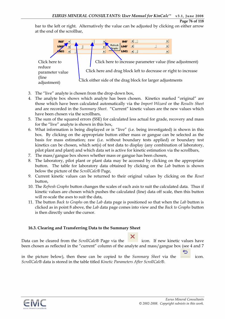
EURUS MINERAL CONSULTANTS: User Manual for KinCalc™ v3.1 , June 2008 Page 76 of 118
Eurus Mineral Consultants © 2002-2008. Copyright subsists in this work.
bar to the left or right. Alternatively the value can be adjusted by clicking on either arrow at the end of the scrollbar,
3. The “live” analyte is chosen from the drop-down box, 4. The analyte box shows which analyte has been chosen. Kinetics marked “original” are
those which have been calculated automatically via the Import Wizard or the Results Sheet and are recorded in the Summary Sheet. “Current” kinetic values are the new values which have been chosen via the scrollbars,
5. The sum of the squared errors (SSE) for calculated less actual for grade, recovery and mass for the “live” analyte is shown in this box,
6. What information is being displayed or is “live” (i.e. being investigated) is shown in this box. By clicking on the appropriate button either mass or gangue can be selected as the basis for mass estimation; raw (i.e. without boundary tests applied) or boundary test kinetics can be chosen, which set(s) of test data to display (any combination of laboratory, pilot plant and plant) and which data set is active for kinetic estimation via the scrollbars,
7. The mass/gangue box shows whether mass or gangue has been chosen, 8. The laboratory, pilot plant or plant data may be accessed by clicking on the appropriate
button. The table for laboratory data obtained by clicking on the Lab button is shown below the picture of the ScrollCalc® Page,
9. Current kinetic values can be returned to their original values by clicking on the Reset button,
10. The Refresh Graphs button changes the scales of each axis to suit the calculated data. Thus if kinetic values are chosen which pushes the calculated (line) data off scale, then this button will re-scale the axes to suit the data,
11. The button Back to Graphs on the Lab data page is positioned so that when the Lab button is clicked as in point 8 above, the Lab data page comes into view and the Back to Graphs button is then directly under the cursor.
16.3. Clearing and Transferring Data to the Summary Sheet
Data can be cleared from the ScrollCalc® Page via the icon. If new kinetic values have been chosen as reflected in the “current” column of the analyte and mass/gangue box (see 4 and 7
in the picture below), then these can be copied to the Summary Sheet via the icon. ScrollCalc® data is stored in the table titled Kinetic Parameters After ScrollCalc®.
Click here to reduce parameter value (fine adjustment)
Click here and drag block left to decrease or right to increase
Click here to increase parameter value (fine adjustment)
Click either side of the drag block for larger adjustments
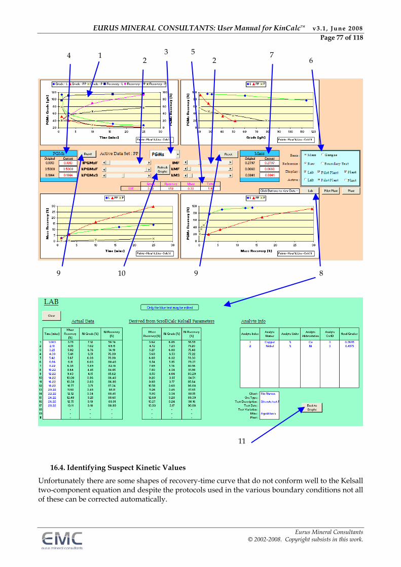
EURUS MINERAL CONSULTANTS: User Manual for KinCalc™ v3.1 , June 2008 Page 77 of 118
Eurus Mineral Consultants © 2002-2008. Copyright subsists in this work.
16.4. Identifying Suspect Kinetic Values
Unfortunately there are some shapes of recovery-time curve that do not conform well to the Kelsall two-component equation and despite the protocols used in the various boundary conditions not all of these can be corrected automatically.
4 2
8
1 7 3 6 2
5
9 10 9
11
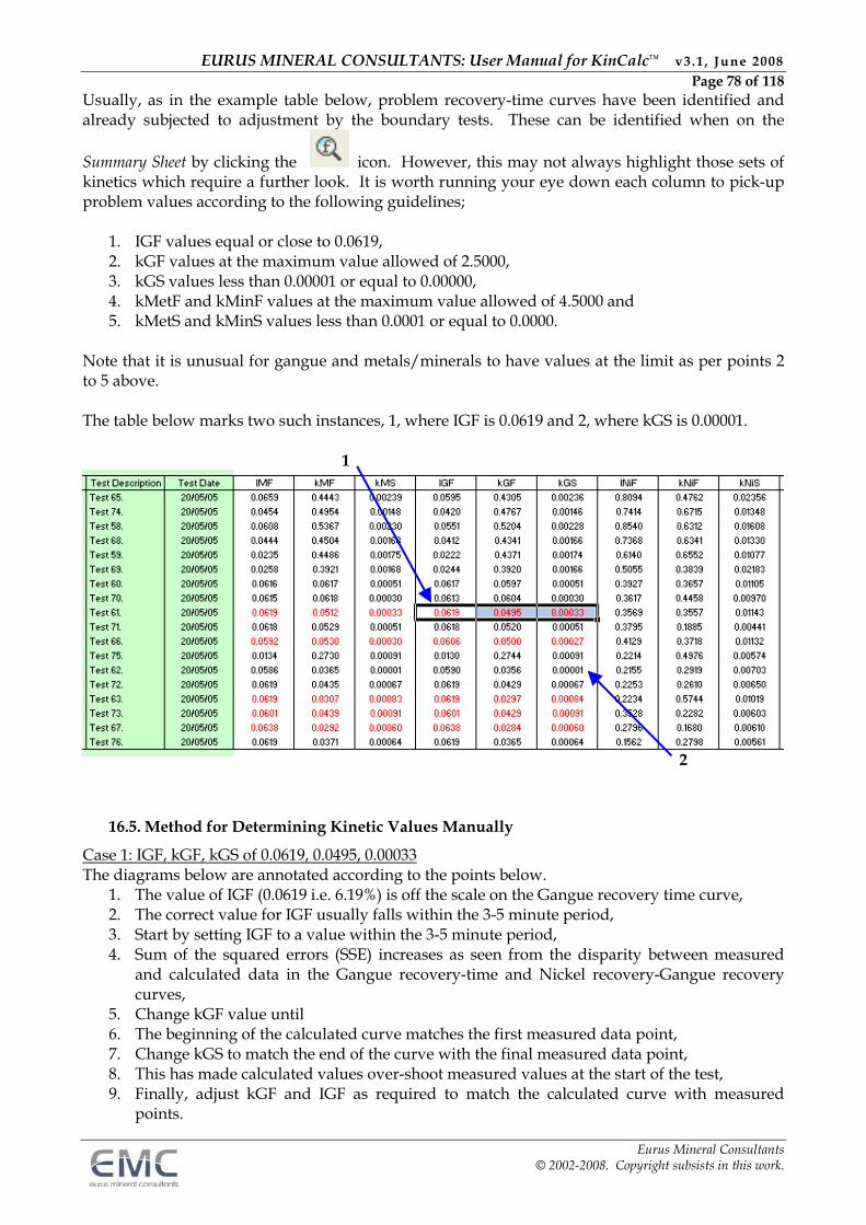
EURUS MINERAL CONSULTANTS: User Manual for KinCalc™ v3.1 , June 2008 Page 78 of 118
Eurus Mineral Consultants © 2002-2008. Copyright subsists in this work.
Usually, as in the example table below, problem recovery-time curves have been identified and already subjected to adjustment by the boundary tests. These can be identified when on the
Summary Sheet by clicking the icon. However, this may not always highlight those sets of kinetics which require a further look. It is worth running your eye down each column to pick-up problem values according to the following guidelines;
1. IGF values equal or close to 0.0619, 2. kGF values at the maximum value allowed of 2.5000, 3. kGS values less than 0.00001 or equal to 0.00000, 4. kMetF and kMinF values at the maximum value allowed of 4.5000 and 5. kMetS and kMinS values less than 0.0001 or equal to 0.0000.
Note that it is unusual for gangue and metals/minerals to have values at the limit as per points 2 to 5 above. The table below marks two such instances, 1, where IGF is 0.0619 and 2, where kGS is 0.00001.
16.5. Method for Determining Kinetic Values Manually
Case 1: IGF, kGF, kGS of 0.0619, 0.0495, 0.00033 The diagrams below are annotated according to the points below.
1. The value of IGF (0.0619 i.e. 6.19%) is off the scale on the Gangue recovery time curve, 2. The correct value for IGF usually falls within the 3-5 minute period, 3. Start by setting IGF to a value within the 3-5 minute period, 4. Sum of the squared errors (SSE) increases as seen from the disparity between measured
and calculated data in the Gangue recovery-time and Nickel recovery-Gangue recovery curves,
5. Change kGF value until 6. The beginning of the calculated curve matches the first measured data point, 7. Change kGS to match the end of the curve with the final measured data point, 8. This has made calculated values over-shoot measured values at the start of the test, 9. Finally, adjust kGF and IGF as required to match the calculated curve with measured
points.
1
2
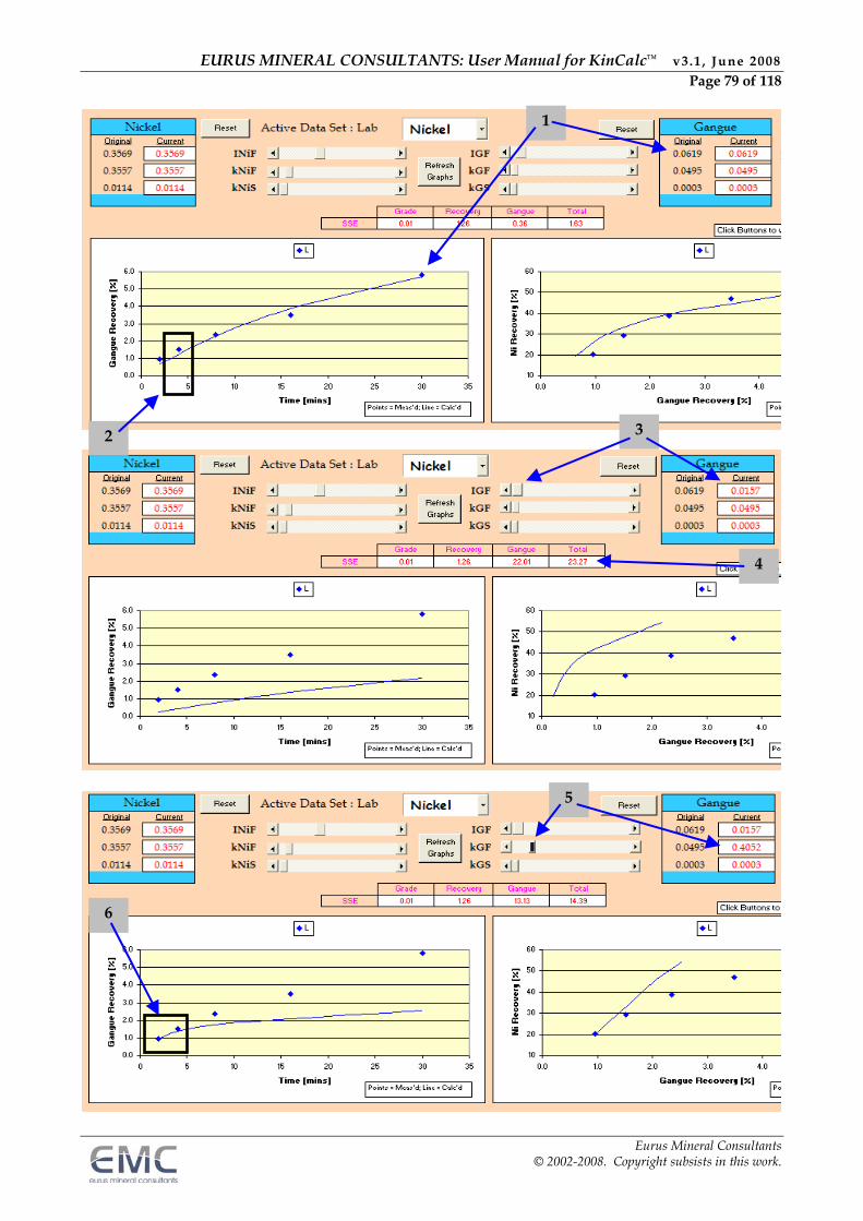
EURUS MINERAL CONSULTANTS: User Manual for KinCalc™ v3.1 , June 2008 Page 79 of 118
Eurus Mineral Consultants © 2002-2008. Copyright subsists in this work.
2
1
3
4
5
6
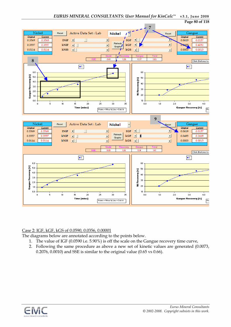
EURUS MINERAL CONSULTANTS: User Manual for KinCalc™ v3.1 , June 2008 Page 80 of 118
Eurus Mineral Consultants © 2002-2008. Copyright subsists in this work.
Case 2: IGF, kGF, kGS of 0.0590, 0.0356, 0.00001 The diagrams below are annotated according to the points below.
1. The value of IGF (0.0590 i.e. 5.90%) is off the scale on the Gangue recovery time curve, 2. Following the same procedure as above a new set of kinetic values are generated (0.0073,
0.2076, 0.0010) and SSE is similar to the original value (0.65 vs 0.66).
7
8
9
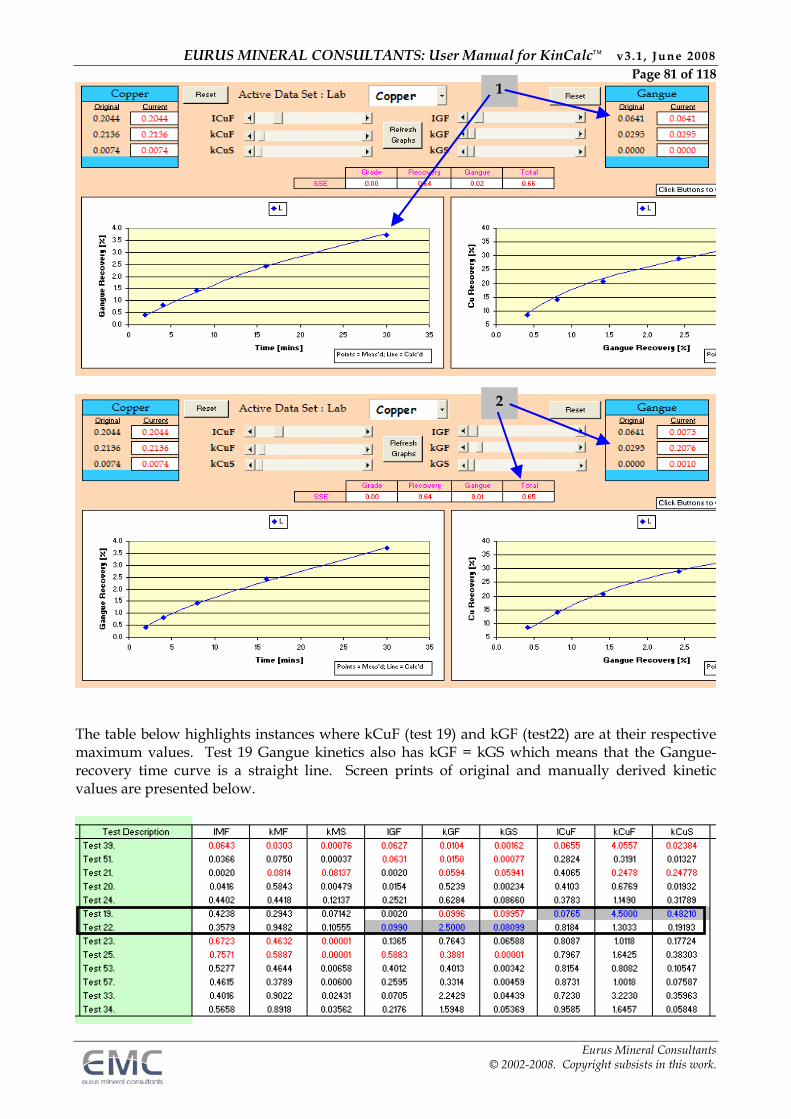
EURUS MINERAL CONSULTANTS: User Manual for KinCalc™ v3.1 , June 2008 Page 81 of 118
Eurus Mineral Consultants © 2002-2008. Copyright subsists in this work.
The table below highlights instances where kCuF (test 19) and kGF (test22) are at their respective maximum values. Test 19 Gangue kinetics also has kGF = kGS which means that the Gangue-recovery time curve is a straight line. Screen prints of original and manually derived kinetic values are presented below.
1
2
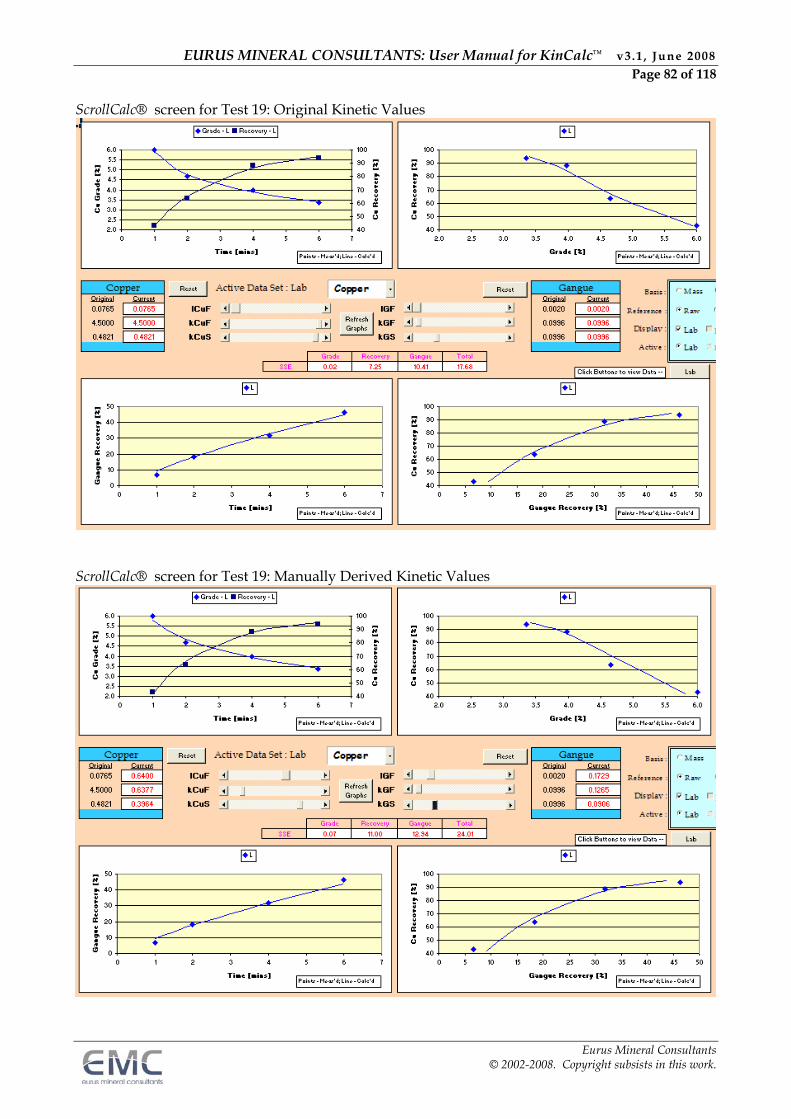
EURUS MINERAL CONSULTANTS: User Manual for KinCalc™ v3.1 , June 2008 Page 82 of 118
Eurus Mineral Consultants © 2002-2008. Copyright subsists in this work.
ScrollCalc® screen for Test 19: Original Kinetic Values
ScrollCalc® screen for Test 19: Manually Derived Kinetic Values
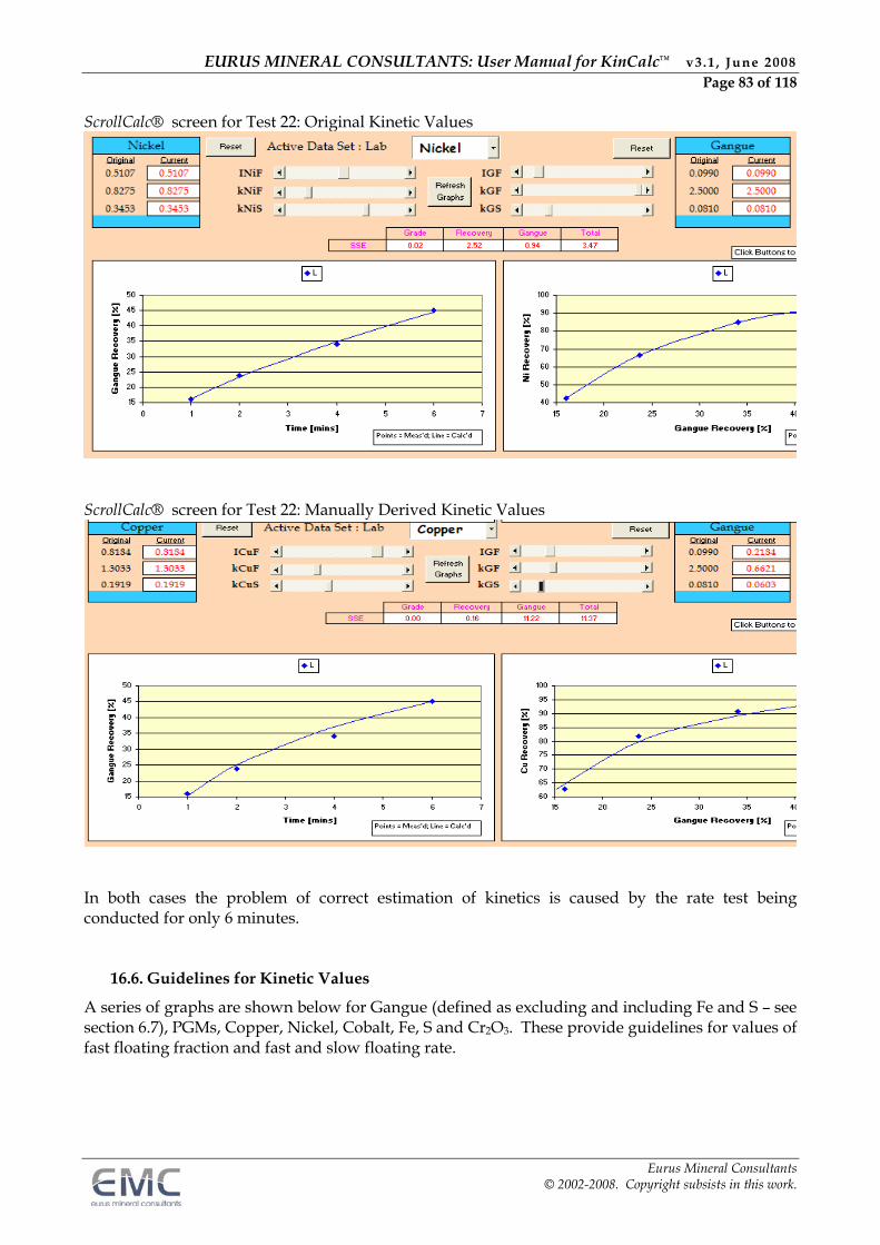
EURUS MINERAL CONSULTANTS: User Manual for KinCalc™ v3.1 , June 2008 Page 83 of 118
Eurus Mineral Consultants © 2002-2008. Copyright subsists in this work.
ScrollCalc® screen for Test 22: Original Kinetic Values
ScrollCalc® screen for Test 22: Manually Derived Kinetic Values
In both cases the problem of correct estimation of kinetics is caused by the rate test being conducted for only 6 minutes.
16.6. Guidelines for Kinetic Values
A series of graphs are shown below for Gangue (defined as excluding and including Fe and S – see section 6.7), PGMs, Copper, Nickel, Cobalt, Fe, S and Cr2O3. These provide guidelines for values of fast floating fraction and fast and slow floating rate.
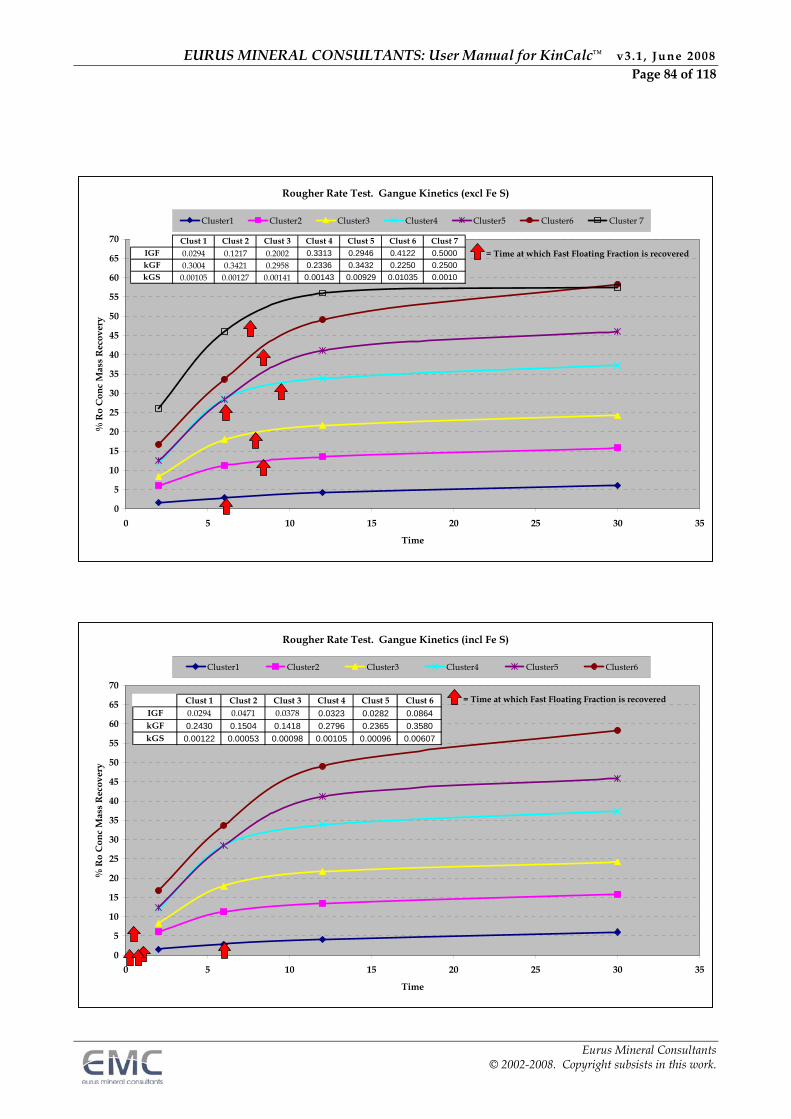
EURUS MINERAL CONSULTANTS: User Manual for KinCalc™ v3.1 , June 2008 Page 84 of 118
Eurus Mineral Consultants © 2002-2008. Copyright subsists in this work.
Rougher Rate Test. Gangue Kinetics (excl Fe S)
0
5
10
15
20
25
30
35
40
45
50
55
60
65
70
0 5 10 15 20 25 30 35
Time
% R
o C
onc
Mas
s R
ecov
ery
Cluster1 Cluster2 Cluster3 Cluster4 Cluster5 Cluster6 Cluster 7
= Time at which Fast Floating Fraction is recoveredClust 1 Clust 2 Clust 3 Clust 4 Clust 5 Clust 6 Clust 7
IGF 0.0294 0.1217 0.2002 0.3313 0.2946 0.4122 0.5000
kGF 0.3004 0.3421 0.2958 0.2336 0.3432 0.2250 0.2500
kGS 0.00105 0.00127 0.00141 0.00143 0.00929 0.01035 0.0010
Rougher Rate Test. Gangue Kinetics (incl Fe S)
0
5
10
15
20
25
30
35
40
45
50
55
60
65
70
0 5 10 15 20 25 30 35
Time
% R
o C
onc
Mas
s R
ecov
ery
Cluster1 Cluster2 Cluster3 Cluster4 Cluster5 Cluster6
Clust 1 Clust 2 Clust 3 Clust 4 Clust 5 Clust 6IGF 0.0294 0.0471 0.0378 0.0323 0.0282 0.0864
kGF 0.2430 0.1504 0.1418 0.2796 0.2365 0.3580
kGS 0.00122 0.00053 0.00098 0.00105 0.00096 0.00607
= Time at which Fast Floating Fraction is recovered
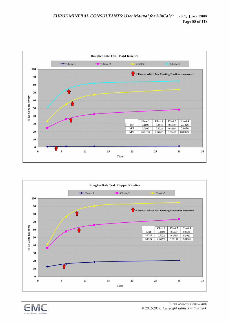
EURUS MINERAL CONSULTANTS: User Manual for KinCalc™ v3.1 , June 2008 Page 85 of 118
Eurus Mineral Consultants © 2002-2008. Copyright subsists in this work.
Rougher Rate Test. PGM Kinetics
0
10
20
30
40
50
60
70
80
90
100
0 5 10 15 20 25 30 35
Time
% R
o C
onc
Rec
over
y
Cluster1 Cluster2 Cluster3 Cluster4
Clust 1 Clust 2 Clust 3 Clust 4IPF 0.1000 0.3815 0.5930 0.7436
kPF 0.0500 0.5024 0.4619 0.6020
kPS 0.01810 0.00699 0.01612 0.02082
= Time at which Fast Floating Fraction is recovered
Rougher Rate Test. Copper Kinetics
0
10
20
30
40
50
60
70
80
90
100
0 5 10 15 20 25 30 35
Time
% R
o C
onc
Rec
over
y
Cluster1 Cluster2 Cluster3
Clust 1 Clust 2 Clust 3ICuF 0.1608 0.6277 0.8531kCuF 0.7724 0.4795 0.3940kCuS 0.00200 0.01191 0.04801
= Time at which Fast Floating Fraction is recovered
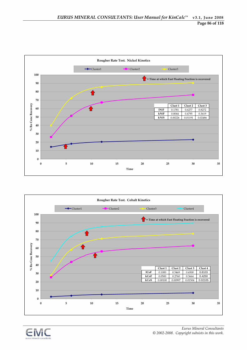
EURUS MINERAL CONSULTANTS: User Manual for KinCalc™ v3.1 , June 2008 Page 86 of 118
Eurus Mineral Consultants © 2002-2008. Copyright subsists in this work.
Rougher Rate Test. Nickel Kinetics
0
10
20
30
40
50
60
70
80
90
100
0 5 10 15 20 25 30 35
Time
% R
o C
onc
Rec
over
y
Cluster1 Cluster2 Cluster3
Clust 1 Clust 2 Clust 3INiF 0.1781 0.6277 0.8272kNiF 0.8044 0.4795 0.3619kNiS 0.00226 0.01191 0.02486
= Time at which Fast Floating Fraction is recovered
Rougher Rate Test. Cobalt Kinetics
0
10
20
30
40
50
60
70
80
90
100
0 5 10 15 20 25 30 35
Time
% R
o C
onc
Rec
over
y
Cluster1 Cluster2 Cluster3 Cluster4
Clust 1 Clust 2 Clust 3 Clust 4ICoF 0.1000 0.5469 0.6500 0.8103
kCoF 0.0500 0.2760 0.3664 0.4250
kCoS 0.00100 0.00997 0.01504 0.02105
= Time at which Fast Floating Fraction is recovered
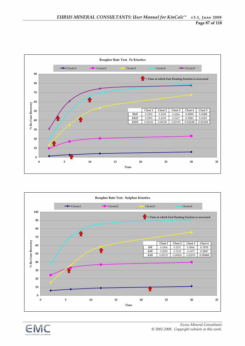
EURUS MINERAL CONSULTANTS: User Manual for KinCalc™ v3.1 , June 2008 Page 87 of 118
Eurus Mineral Consultants © 2002-2008. Copyright subsists in this work.
Rougher Rate Test. Fe Kinetics
0
10
20
30
40
50
60
70
80
90
0 5 10 15 20 25 30 35
Time
% R
o C
onc
Rec
over
y
Cluster1 Cluster2 Cluster3 Cluster4 Cluster5
Clust 1 Clust 2 Clust 3 Clust 4 Clust 5IFeF 0.0292 0.1838 0.4266 0.6550 0.4266
kFeF 0.2976 0.4339 0.2167 0.2561 0.2167
kFeS 0.00102 0.00198 0.02159 0.03108 0.02159
= Time at which Fast Floating Fraction is recovered
Rougher Rate Test. Sulphur Kinetics
0
10
20
30
40
50
60
70
80
90
100
0 5 10 15 20 25 30 35
Time
% R
o C
onc
Rec
over
y
Cluster1 Cluster2 Cluster3 Cluster4
Clust 1 Clust 2 Clust 3 Clust 4ISF 0.1006 0.3271 0.5884 0.7876
kSF 0.2859 0.3139 0.1475 0.3947
kSS 0.00137 0.09830 0.02978 0.05668
= Time at which Fast Floating Fraction is recovered
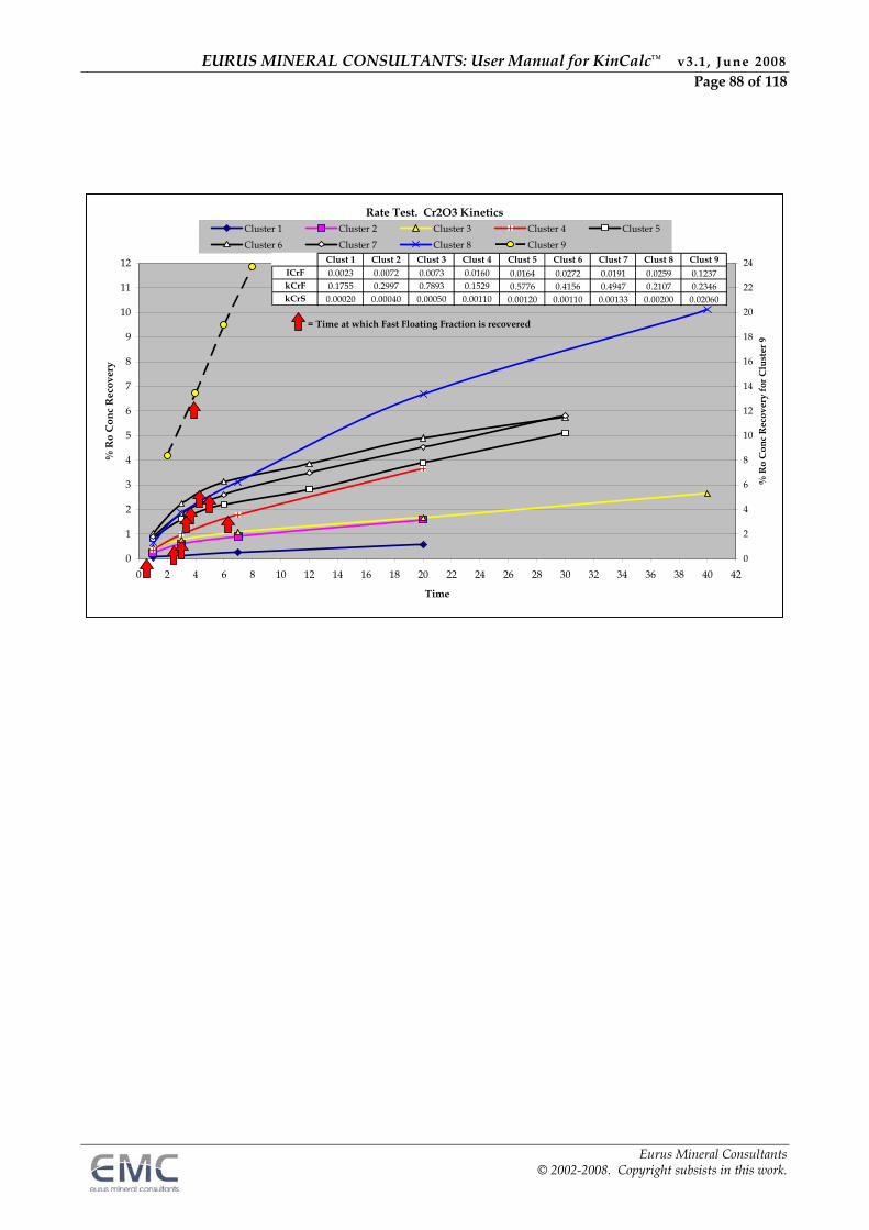
EURUS MINERAL CONSULTANTS: User Manual for KinCalc™ v3.1 , June 2008 Page 88 of 118
Eurus Mineral Consultants © 2002-2008. Copyright subsists in this work.
Rate Test. Cr2O3 Kinetics
0
1
2
3
4
5
6
7
8
9
10
11
12
0 2 4 6 8 10 12 14 16 18 20 22 24 26 28 30 32 34 36 38 40 42
Time
% R
o C
onc
Rec
over
y
0
2
4
6
8
10
12
14
16
18
20
22
24
% R
o C
onc
Rec
over
y fo
r C
lust
er 9
Cluster 1 Cluster 2 Cluster 3 Cluster 4 Cluster 5
Cluster 6 Cluster 7 Cluster 8 Cluster 9
= Time at which Fast Floating Fraction is recovered
Clust 1 Clust 2 Clust 3 Clust 4 Clust 5 Clust 6 Clust 7 Clust 8 Clust 9ICrF 0.0023 0.0072 0.0073 0.0160 0.0164 0.0272 0.0191 0.0259 0.1237kCrF 0.1755 0.2997 0.7893 0.1529 0.5776 0.4156 0.4947 0.2107 0.2346kCrS 0.00020 0.00040 0.00050 0.00110 0.00120 0.00110 0.00133 0.00200 0.02060
EURUS MINERAL CONSULTANTS: User Manual for KinCalc™ v3.1 , June 2008 Page 89 of 118
Eurus Mineral Consultants © 2002-2008. Copyright subsists in this work.
17. ACCESS or SQL DATABASE
Functions available: 1. Importing of data back into the Summary Sheet 2. Queries and searches of the database by customised selection tables
Diagrams highlighting various points detailed below can be found towards the end of this section.
17.1. Posting Data to the Access or SQL Database
Single data records can be posted to the Access or SQL Database by highlighting the required data
and clicking the icon. If all data on the Summary Sheet is to be posted to the Access or SQL
Database then this is done by clicking the icon.
17.2. Importing Data from the Access or SQL Database into the Summary Sheet
This is done by clicking on the icon. As per the dialog boxes below this shows an import table with two tabs, Test Info and Other Info. The import table allows the user to select data from a variety of categories; Client, Mine, Ore Type, Plant, Analytes, Other Parameters and Stream Names. The number of matching records for the particular combination of categories chosen is shown at the bottom left of the import table (in this case it is 2 matching records). On the Test Info tab the Data Source may be chosen – i.e. laboratory, pilot plant or plant data or any combination and the Test Date may be chosen. Test date or dates may be entered as shown below. When the required categories have been selected then click the Import button to load the data into the Summary Sheet.
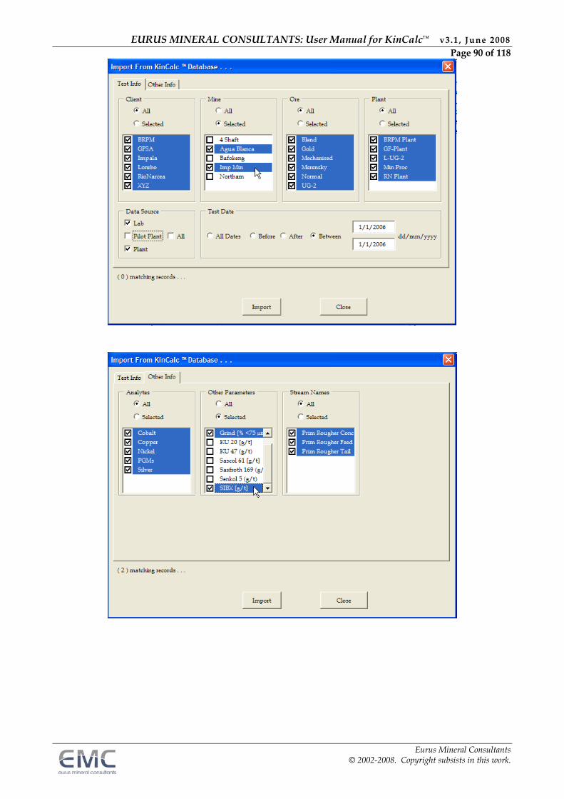
EURUS MINERAL CONSULTANTS: User Manual for KinCalc™ v3.1 , June 2008 Page 90 of 118
Eurus Mineral Consultants © 2002-2008. Copyright subsists in this work.
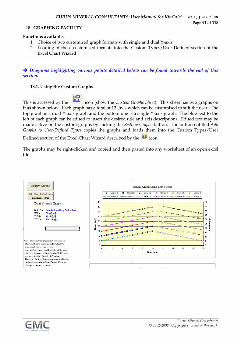
EURUS MINERAL CONSULTANTS: User Manual for KinCalc™ v3.1 , June 2008 Page 91 of 118
Eurus Mineral Consultants © 2002-2008. Copyright subsists in this work.
18. GRAPHING FACILITY
Functions available: 1. Choice of two customised graph formats with single and dual Y-axis 2. Loading of these customised formats into the Custom Types/User Defined section of the
Excel Chart Wizard Diagrams highlighting various points detailed below can be found towards the end of this section.
18.1. Using the Custom Graphs
This is accessed by the icon (show the Custom Graphs Sheet). This sheet has two graphs on it as shown below. Each graph has a total of 12 lines which can be customised to suit the user. The top graph is a dual Y-axis graph and the bottom one is a single Y-axis graph. The blue text to the left of each graph can be edited to insert the desired title and axis descriptions. Edited text may be made active on the custom graphs by clicking the Redraw Graphs button. The button entitled Add Graphs to User-Defined Types copies the graphs and loads them into the Custom Types/User
Defined section of the Excel Chart Wizard described by the icon. The graphs may be right-clicked and copied and then pasted into any worksheet of an open excel file.
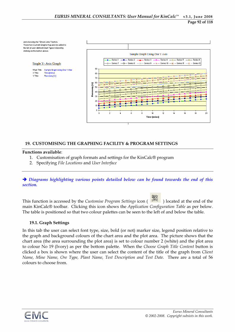
EURUS MINERAL CONSULTANTS: User Manual for KinCalc™ v3.1 , June 2008 Page 92 of 118
Eurus Mineral Consultants © 2002-2008. Copyright subsists in this work.
19. CUSTOMISING THE GRAPHING FACILITY & PROGRAM SETTINGS
Functions available: 1. Customisation of graph formats and settings for the KinCalc® program 2. Specifying File Locations and User Interface
Diagrams highlighting various points detailed below can be found towards the end of this section.
This function is accessed by the Customise Program Settings icon ( ) located at the end of the main KinCalc® toolbar. Clicking this icon shows the Application Configuration Table as per below. The table is positioned so that two colour palettes can be seen to the left of and below the table.
19.1. Graph Settings
In this tab the user can select font type, size, bold (or not) marker size, legend position relative to the graph and background colours of the chart area and the plot area. The picture shows that the chart area (the area surrounding the plot area) is set to colour number 2 (white) and the plot area to colour No 19 (Ivory) as per the bottom palette. When the Choose Graph Title Content button is clicked a box is shown where the user can select the content of the title of the graph from Client Name, Mine Name, Ore Type, Plant Name, Test Description and Test Date. There are a total of 56 colours to choose from.
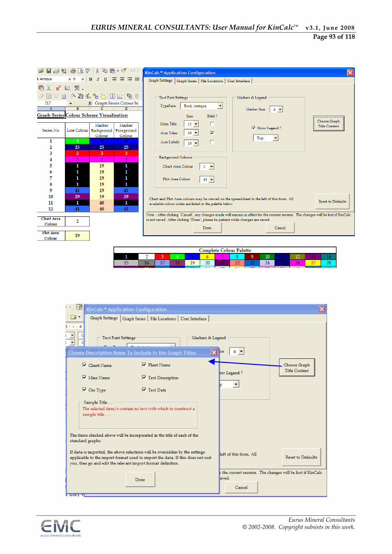
EURUS MINERAL CONSULTANTS: User Manual for KinCalc™ v3.1 , June 2008 Page 93 of 118
Eurus Mineral Consultants © 2002-2008. Copyright subsists in this work.
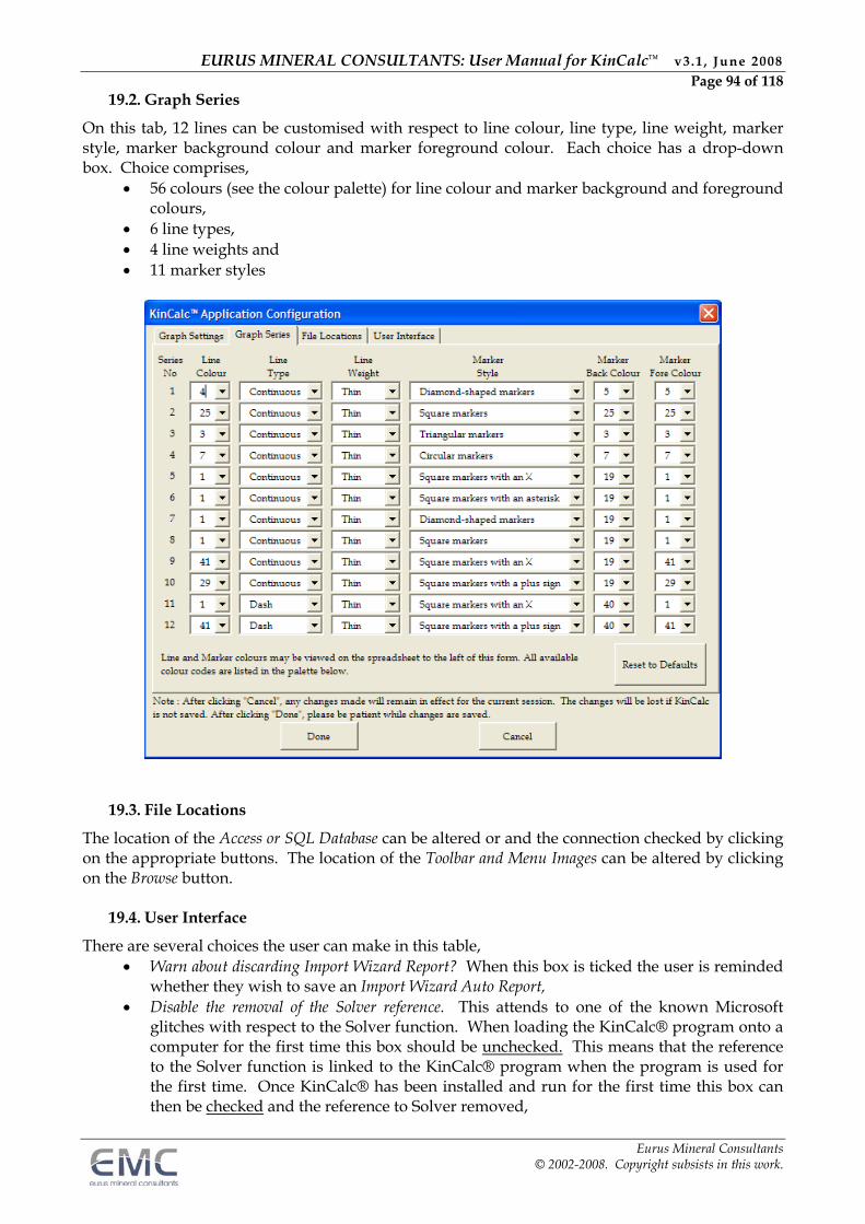
EURUS MINERAL CONSULTANTS: User Manual for KinCalc™ v3.1 , June 2008 Page 94 of 118
Eurus Mineral Consultants © 2002-2008. Copyright subsists in this work.
19.2. Graph Series
On this tab, 12 lines can be customised with respect to line colour, line type, line weight, marker style, marker background colour and marker foreground colour. Each choice has a drop-down box. Choice comprises,
56 colours (see the colour palette) for line colour and marker background and foreground colours,
6 line types, 4 line weights and 11 marker styles
19.3. File Locations
The location of the Access or SQL Database can be altered or and the connection checked by clicking on the appropriate buttons. The location of the Toolbar and Menu Images can be altered by clicking on the Browse button.
19.4. User Interface
There are several choices the user can make in this table, Warn about discarding Import Wizard Report? When this box is ticked the user is reminded
whether they wish to save an Import Wizard Auto Report, Disable the removal of the Solver reference. This attends to one of the known Microsoft
glitches with respect to the Solver function. When loading the KinCalc® program onto a computer for the first time this box should be unchecked. This means that the reference to the Solver function is linked to the KinCalc® program when the program is used for the first time. Once KinCalc® has been installed and run for the first time this box can then be checked and the reference to Solver removed,
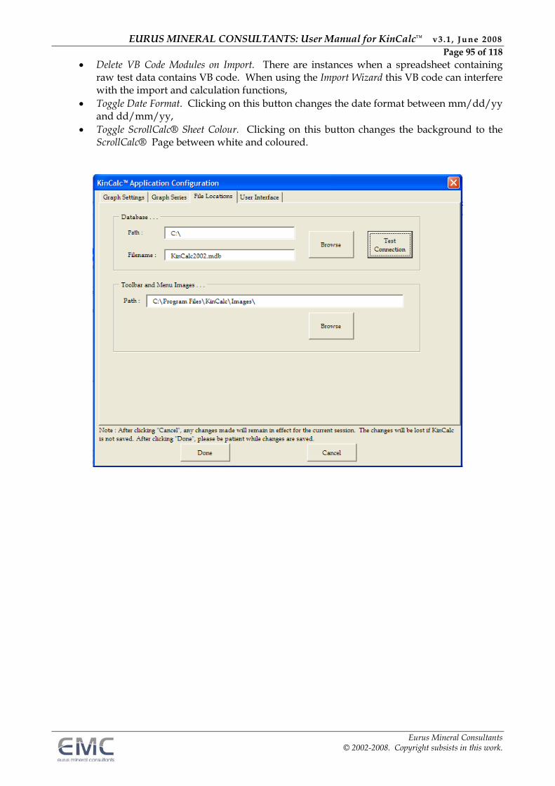
EURUS MINERAL CONSULTANTS: User Manual for KinCalc™ v3.1 , June 2008 Page 95 of 118
Eurus Mineral Consultants © 2002-2008. Copyright subsists in this work.
Delete VB Code Modules on Import. There are instances when a spreadsheet containing raw test data contains VB code. When using the Import Wizard this VB code can interfere with the import and calculation functions,
Toggle Date Format. Clicking on this button changes the date format between mm/dd/yy and dd/mm/yy,
Toggle ScrollCalc® Sheet Colour. Clicking on this button changes the background to the ScrollCalc® Page between white and coloured.
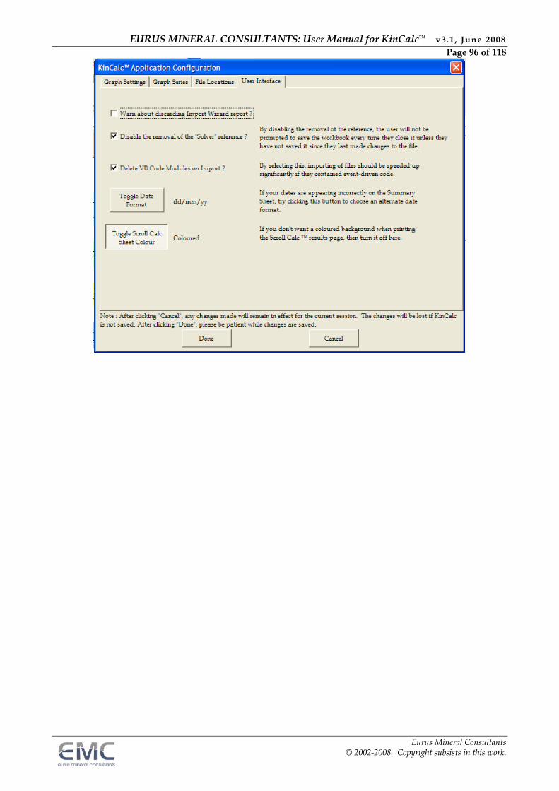
EURUS MINERAL CONSULTANTS: User Manual for KinCalc™ v3.1 , June 2008 Page 96 of 118
Eurus Mineral Consultants © 2002-2008. Copyright subsists in this work.
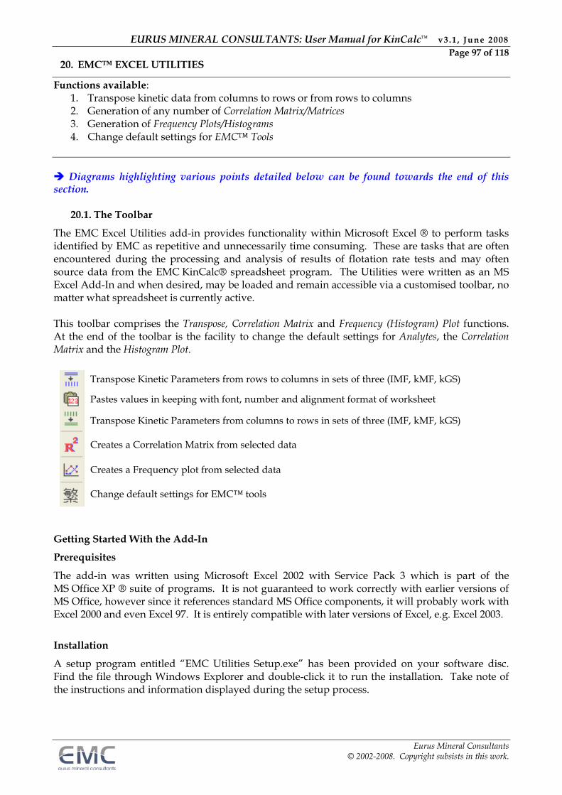
EURUS MINERAL CONSULTANTS: User Manual for KinCalc™ v3.1 , June 2008 Page 97 of 118
Eurus Mineral Consultants © 2002-2008. Copyright subsists in this work.
20. EMC™ EXCEL UTILITIES
Functions available: 1. Transpose kinetic data from columns to rows or from rows to columns 2. Generation of any number of Correlation Matrix/Matrices 3. Generation of Frequency Plots/Histograms 4. Change default settings for EMC™ Tools
Diagrams highlighting various points detailed below can be found towards the end of this section.
20.1. The Toolbar
The EMC Excel Utilities add-in provides functionality within Microsoft Excel ® to perform tasks identified by EMC as repetitive and unnecessarily time consuming. These are tasks that are often encountered during the processing and analysis of results of flotation rate tests and may often source data from the EMC KinCalc® spreadsheet program. The Utilities were written as an MS Excel Add-In and when desired, may be loaded and remain accessible via a customised toolbar, no matter what spreadsheet is currently active. This toolbar comprises the Transpose, Correlation Matrix and Frequency (Histogram) Plot functions. At the end of the toolbar is the facility to change the default settings for Analytes, the Correlation Matrix and the Histogram Plot.
Transpose Kinetic Parameters from rows to columns in sets of three (IMF, kMF, kGS)
Pastes values in keeping with font, number and alignment format of worksheet
Transpose Kinetic Parameters from columns to rows in sets of three (IMF, kMF, kGS)
Creates a Correlation Matrix from selected data
Creates a Frequency plot from selected data
Change default settings for EMC™ tools
Getting Started With the Add-In
Prerequisites
The add-in was written using Microsoft Excel 2002 with Service Pack 3 which is part of the MS Office XP ® suite of programs. It is not guaranteed to work correctly with earlier versions of MS Office, however since it references standard MS Office components, it will probably work with Excel 2000 and even Excel 97. It is entirely compatible with later versions of Excel, e.g. Excel 2003.
Installation
A setup program entitled “EMC Utilities Setup.exe” has been provided on your software disc. Find the file through Windows Explorer and double-click it to run the installation. Take note of the instructions and information displayed during the setup process.
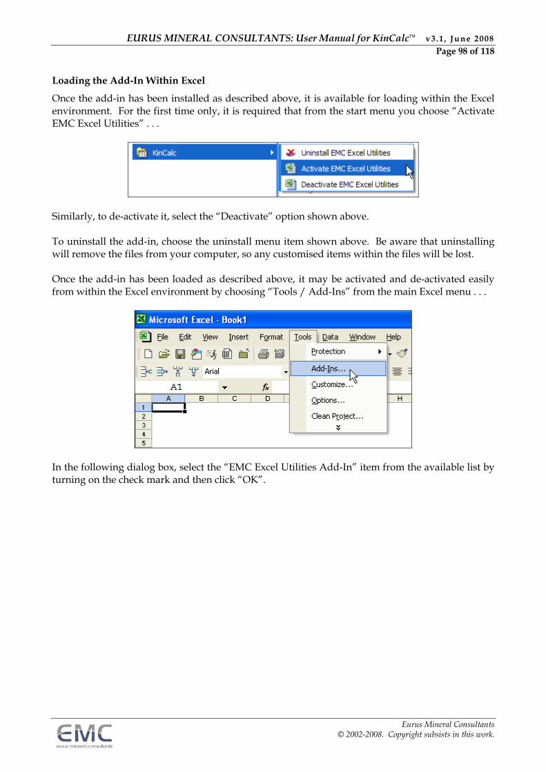
EURUS MINERAL CONSULTANTS: User Manual for KinCalc™ v3.1 , June 2008 Page 98 of 118
Eurus Mineral Consultants © 2002-2008. Copyright subsists in this work.
Loading the Add-In Within Excel
Once the add-in has been installed as described above, it is available for loading within the Excel environment. For the first time only, it is required that from the start menu you choose “Activate EMC Excel Utilities” . . .
Similarly, to de-activate it, select the “Deactivate” option shown above. To uninstall the add-in, choose the uninstall menu item shown above. Be aware that uninstalling will remove the files from your computer, so any customised items within the files will be lost. Once the add-in has been loaded as described above, it may be activated and de-activated easily from within the Excel environment by choosing “Tools / Add-Ins” from the main Excel menu . . .
In the following dialog box, select the “EMC Excel Utilities Add-In” item from the available list by turning on the check mark and then click “OK”.
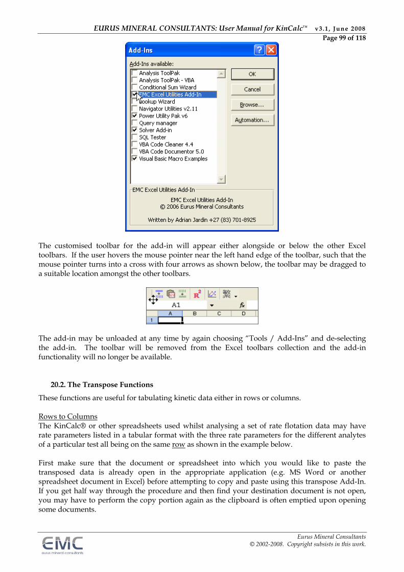
EURUS MINERAL CONSULTANTS: User Manual for KinCalc™ v3.1 , June 2008 Page 99 of 118
Eurus Mineral Consultants © 2002-2008. Copyright subsists in this work.
The customised toolbar for the add-in will appear either alongside or below the other Excel toolbars. If the user hovers the mouse pointer near the left hand edge of the toolbar, such that the mouse pointer turns into a cross with four arrows as shown below, the toolbar may be dragged to a suitable location amongst the other toolbars.
The add-in may be unloaded at any time by again choosing “Tools / Add-Ins” and de-selecting the add-in. The toolbar will be removed from the Excel toolbars collection and the add-in functionality will no longer be available.
20.2. The Transpose Functions
These functions are useful for tabulating kinetic data either in rows or columns. Rows to Columns The KinCalc® or other spreadsheets used whilst analysing a set of rate flotation data may have rate parameters listed in a tabular format with the three rate parameters for the different analytes of a particular test all being on the same row as shown in the example below. First make sure that the document or spreadsheet into which you would like to paste the transposed data is already open in the appropriate application (e.g. MS Word or another spreadsheet document in Excel) before attempting to copy and paste using this transpose Add-In. If you get half way through the procedure and then find your destination document is not open, you may have to perform the copy portion again as the clipboard is often emptied upon opening some documents.
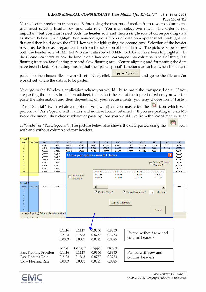
EURUS MINERAL CONSULTANTS: User Manual for KinCalc™ v3.1 , June 2008 Page 100 of 118
Eurus Mineral Consultants © 2002-2008. Copyright subsists in this work.
Next select the region to transpose. Before using the transpose function from rows to columns the user must select a header row and data row. You must select two rows. The order is not important, but you must select both the header row and then a single row of corresponding data as shown below. To highlight two non-contiguous blocks of data on a spreadsheet, highlight the first and then hold down the CTRL key while highlighting the second row. Selection of the header row must be done as a separate action from the selection of the data row. The picture below shows both the header row of IMF to kNiS and data row of 0.1416 to 0.00250 have been highlighted. In the Choose Your Options box the kinetic data has been rearranged into columns in sets of three; fast floating fraction, fast floating rate and slow floating rate. Centre aligning and formatting the data have been ticked. Formatting means that the “paste special” functions are active when the data is
pasted to the chosen file or worksheet. Next, click and go to the file and/or worksheet where the data is to be pasted. Next, go to the Windows application where you would like to paste the transposed data. If you are pasting the results into a spreadsheet, then select the cell at the top-left of where you want to paste the information and then depending on your requirements, you may choose from “Paste”,
“Paste Special” (with whatever options you want) or you may click the icon which will perform a “Paste Special with values and number format retained”. If you are pasting into an MS Word document, then choose whatever paste options you would like from the Word menus, such
as “Paste” or “Paste Special”. The picture below also shows the data pasted using the icon with and without column and row headers.
0.1416 0.1117 0.9356 0.88330.2133 0.1863 0.8752 0.32530.0003 0.0001 0.0325 0.0025
Mass Gangue Copper NickelFast Floating Fraction 0.1416 0.1117 0.9356 0.8833Fast Floating Rate 0.2133 0.1863 0.8752 0.3253Slow Floating Rate 0.0003 0.0001 0.0325 0.0025
Pasted without row and column headers
Pasted with row and column headers
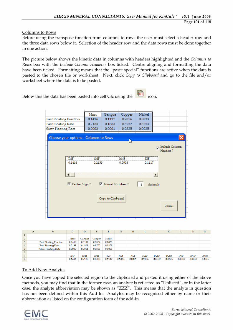
EURUS MINERAL CONSULTANTS: User Manual for KinCalc™ v3.1 , June 2008 Page 101 of 118
Eurus Mineral Consultants © 2002-2008. Copyright subsists in this work.
Columns to Rows Before using the transpose function from columns to rows the user must select a header row and the three data rows below it. Selection of the header row and the data rows must be done together in one action. The picture below shows the kinetic data in columns with headers highlighted and the Columns to Rows box with the Include Column Headers? box ticked. Centre aligning and formatting the data have been ticked. Formatting means that the “paste special” functions are active when the data is pasted to the chosen file or worksheet. Next, click Copy to Clipboard and go to the file and/or worksheet where the data is to be pasted.
Below this the data has been pasted into cell C& using the icon.
To Add New Analytes
Once you have copied the selected region to the clipboard and pasted it using either of the above methods, you may find that in the former case, an analyte is reflected as “Unlisted”, or in the latter case, the analyte abbreviation may be shown as “ZZZ”. This means that the analyte in question has not been defined within this Add-In. Analytes may be recognised either by name or their abbreviation as listed on the configuration form of the add-in.
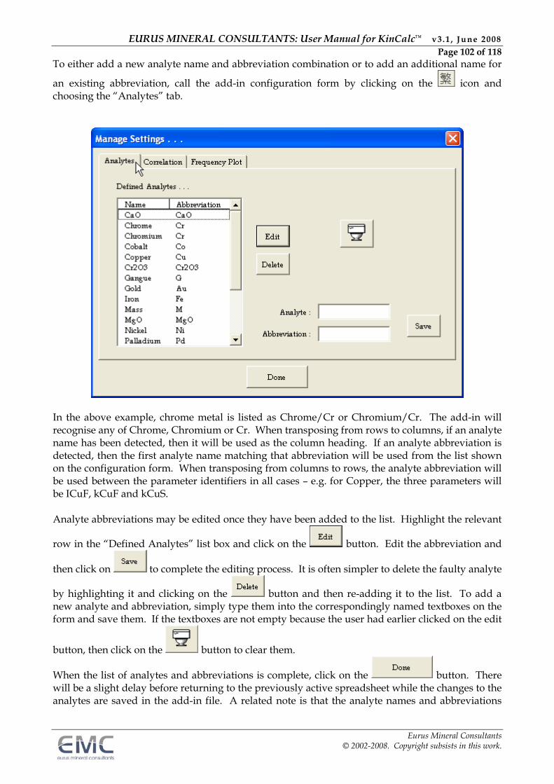
EURUS MINERAL CONSULTANTS: User Manual for KinCalc™ v3.1 , June 2008 Page 102 of 118
Eurus Mineral Consultants © 2002-2008. Copyright subsists in this work.
To either add a new analyte name and abbreviation combination or to add an additional name for
an existing abbreviation, call the add-in configuration form by clicking on the icon and choosing the “Analytes” tab.
In the above example, chrome metal is listed as Chrome/Cr or Chromium/Cr. The add-in will recognise any of Chrome, Chromium or Cr. When transposing from rows to columns, if an analyte name has been detected, then it will be used as the column heading. If an analyte abbreviation is detected, then the first analyte name matching that abbreviation will be used from the list shown on the configuration form. When transposing from columns to rows, the analyte abbreviation will be used between the parameter identifiers in all cases – e.g. for Copper, the three parameters will be ICuF, kCuF and kCuS. Analyte abbreviations may be edited once they have been added to the list. Highlight the relevant
row in the “Defined Analytes” list box and click on the button. Edit the abbreviation and
then click on to complete the editing process. It is often simpler to delete the faulty analyte
by highlighting it and clicking on the button and then re-adding it to the list. To add a new analyte and abbreviation, simply type them into the correspondingly named textboxes on the form and save them. If the textboxes are not empty because the user had earlier clicked on the edit
button, then click on the button to clear them.
When the list of analytes and abbreviations is complete, click on the button. There will be a slight delay before returning to the previously active spreadsheet while the changes to the analytes are saved in the add-in file. A related note is that the analyte names and abbreviations
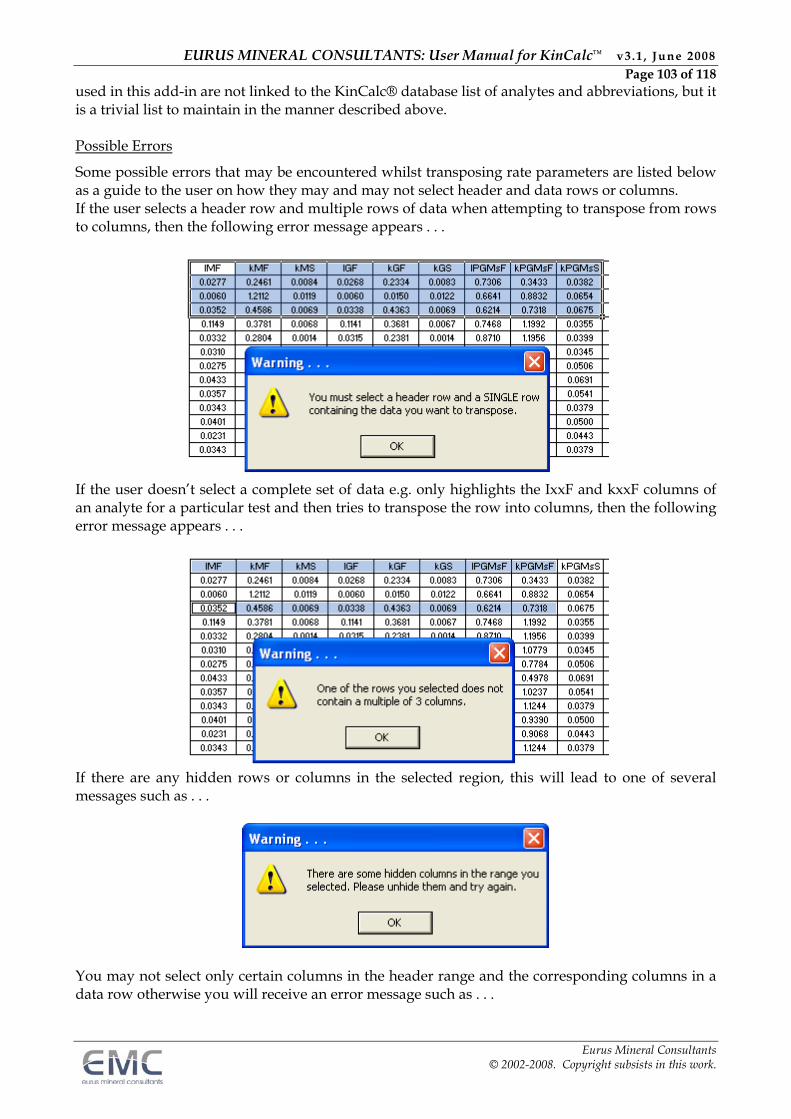
EURUS MINERAL CONSULTANTS: User Manual for KinCalc™ v3.1 , June 2008 Page 103 of 118
Eurus Mineral Consultants © 2002-2008. Copyright subsists in this work.
used in this add-in are not linked to the KinCalc® database list of analytes and abbreviations, but it is a trivial list to maintain in the manner described above. Possible Errors
Some possible errors that may be encountered whilst transposing rate parameters are listed below as a guide to the user on how they may and may not select header and data rows or columns. If the user selects a header row and multiple rows of data when attempting to transpose from rows to columns, then the following error message appears . . .
If the user doesn’t select a complete set of data e.g. only highlights the IxxF and kxxF columns of an analyte for a particular test and then tries to transpose the row into columns, then the following error message appears . . .
If there are any hidden rows or columns in the selected region, this will lead to one of several messages such as . . .
You may not select only certain columns in the header range and the corresponding columns in a data row otherwise you will receive an error message such as . . .
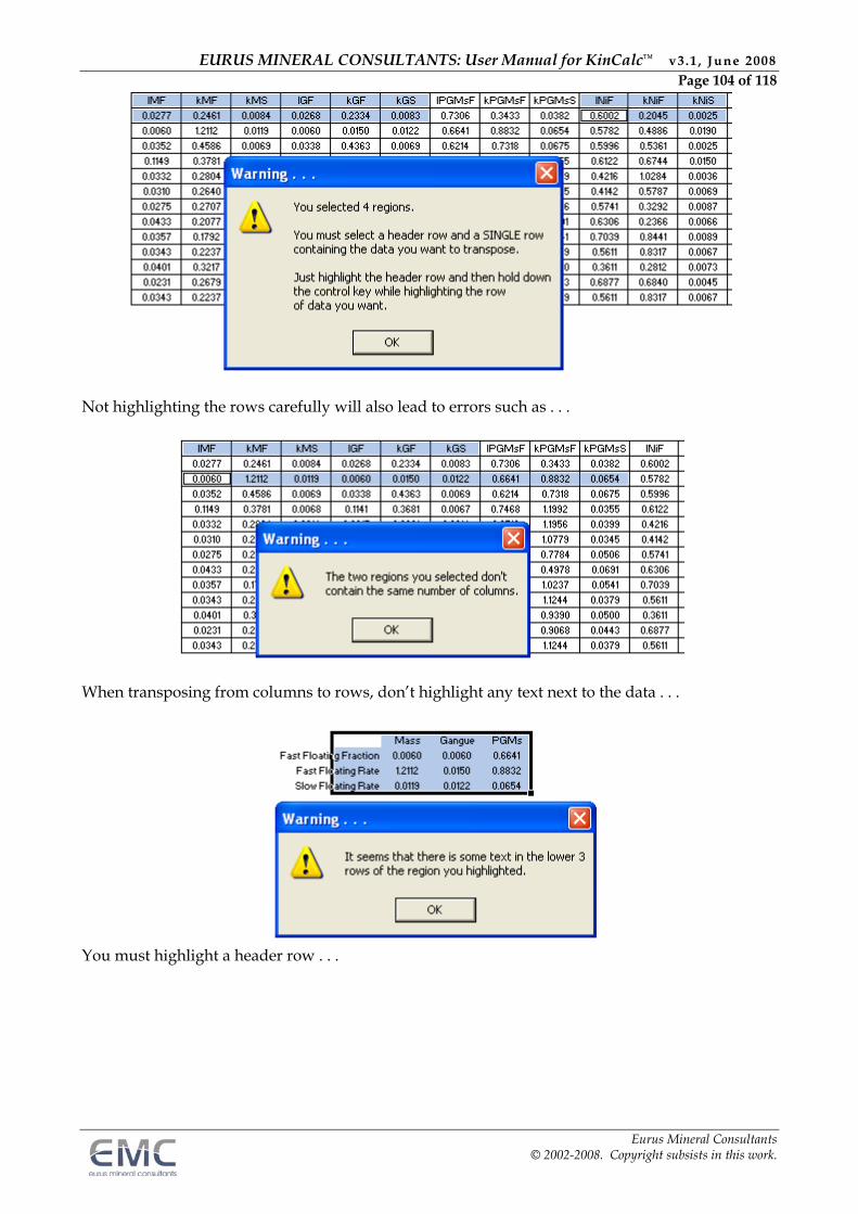
EURUS MINERAL CONSULTANTS: User Manual for KinCalc™ v3.1 , June 2008 Page 104 of 118
Eurus Mineral Consultants © 2002-2008. Copyright subsists in this work.
Not highlighting the rows carefully will also lead to errors such as . . .
When transposing from columns to rows, don’t highlight any text next to the data . . .
You must highlight a header row . . .
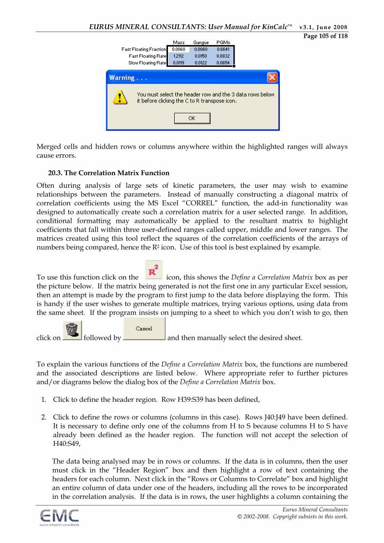
EURUS MINERAL CONSULTANTS: User Manual for KinCalc™ v3.1 , June 2008 Page 105 of 118
Eurus Mineral Consultants © 2002-2008. Copyright subsists in this work.
Merged cells and hidden rows or columns anywhere within the highlighted ranges will always cause errors.
20.3. The Correlation Matrix Function
Often during analysis of large sets of kinetic parameters, the user may wish to examine relationships between the parameters. Instead of manually constructing a diagonal matrix of correlation coefficients using the MS Excel “CORREL” function, the add-in functionality was designed to automatically create such a correlation matrix for a user selected range. In addition, conditional formatting may automatically be applied to the resultant matrix to highlight coefficients that fall within three user-defined ranges called upper, middle and lower ranges. The matrices created using this tool reflect the squares of the correlation coefficients of the arrays of numbers being compared, hence the R2 icon. Use of this tool is best explained by example.
To use this function click on the icon, this shows the Define a Correlation Matrix box as per the picture below. If the matrix being generated is not the first one in any particular Excel session, then an attempt is made by the program to first jump to the data before displaying the form. This is handy if the user wishes to generate multiple matrices, trying various options, using data from the same sheet. If the program insists on jumping to a sheet to which you don’t wish to go, then
click on followed by and then manually select the desired sheet. To explain the various functions of the Define a Correlation Matrix box, the functions are numbered and the associated descriptions are listed below. Where appropriate refer to further pictures and/or diagrams below the dialog box of the Define a Correlation Matrix box.
1. Click to define the header region. Row H39:S39 has been defined, 2. Click to define the rows or columns (columns in this case). Rows J40:J49 have been defined.
It is necessary to define only one of the columns from H to S because columns H to S have already been defined as the header region. The function will not accept the selection of H40:S49,
The data being analysed may be in rows or columns. If the data is in columns, then the user must click in the “Header Region” box and then highlight a row of text containing the headers for each column. Next click in the “Rows or Columns to Correlate” box and highlight an entire column of data under one of the headers, including all the rows to be incorporated in the correlation analysis. If the data is in rows, the user highlights a column containing the
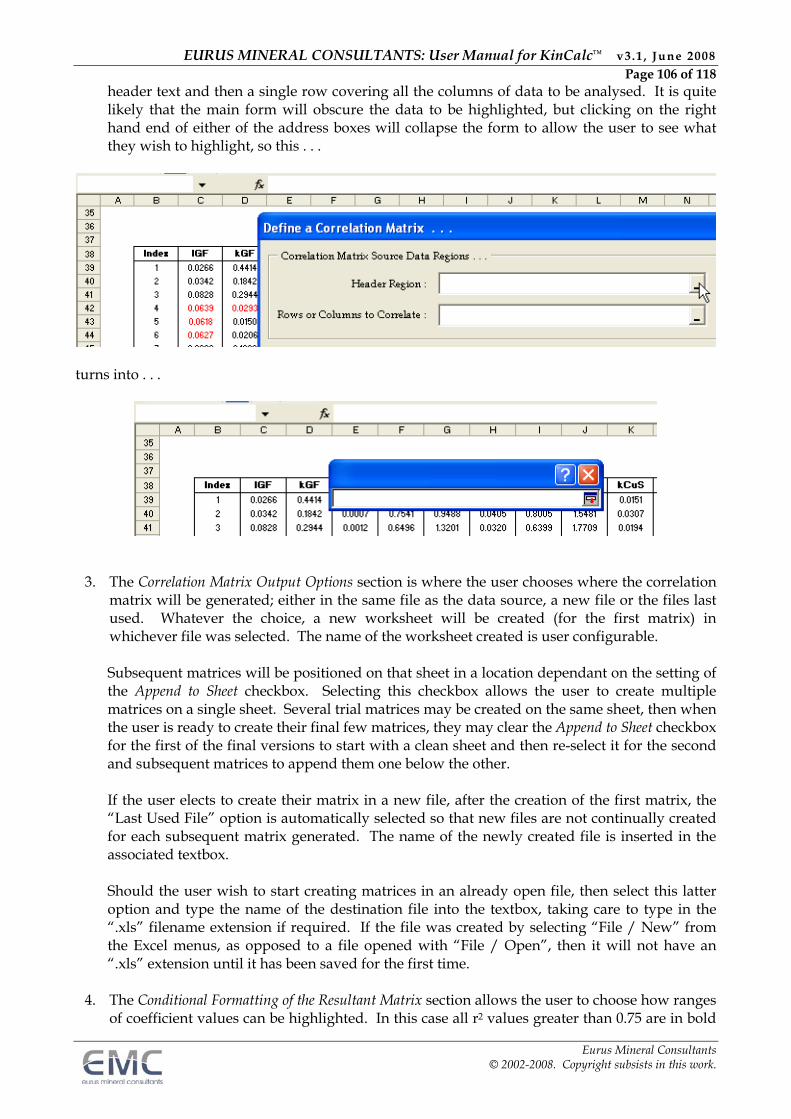
EURUS MINERAL CONSULTANTS: User Manual for KinCalc™ v3.1 , June 2008 Page 106 of 118
Eurus Mineral Consultants © 2002-2008. Copyright subsists in this work.
header text and then a single row covering all the columns of data to be analysed. It is quite likely that the main form will obscure the data to be highlighted, but clicking on the right hand end of either of the address boxes will collapse the form to allow the user to see what they wish to highlight, so this . . .
turns into . . .
3. The Correlation Matrix Output Options section is where the user chooses where the correlation matrix will be generated; either in the same file as the data source, a new file or the files last used. Whatever the choice, a new worksheet will be created (for the first matrix) in whichever file was selected. The name of the worksheet created is user configurable.
Subsequent matrices will be positioned on that sheet in a location dependant on the setting of the Append to Sheet checkbox. Selecting this checkbox allows the user to create multiple matrices on a single sheet. Several trial matrices may be created on the same sheet, then when the user is ready to create their final few matrices, they may clear the Append to Sheet checkbox for the first of the final versions to start with a clean sheet and then re-select it for the second and subsequent matrices to append them one below the other.
If the user elects to create their matrix in a new file, after the creation of the first matrix, the “Last Used File” option is automatically selected so that new files are not continually created for each subsequent matrix generated. The name of the newly created file is inserted in the associated textbox. Should the user wish to start creating matrices in an already open file, then select this latter option and type the name of the destination file into the textbox, taking care to type in the “.xls” filename extension if required. If the file was created by selecting “File / New” from the Excel menus, as opposed to a file opened with “File / Open”, then it will not have an “.xls” extension until it has been saved for the first time.
4. The Conditional Formatting of the Resultant Matrix section allows the user to choose how ranges
of coefficient values can be highlighted. In this case all r2 values greater than 0.75 are in bold
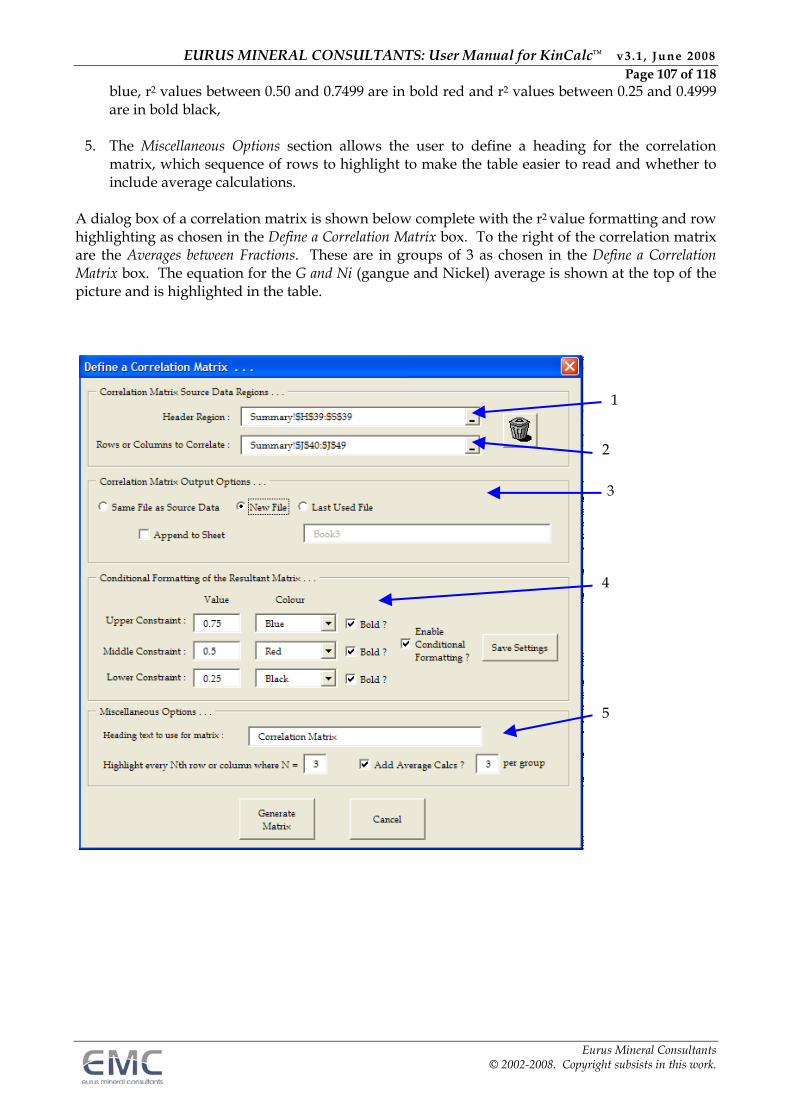
EURUS MINERAL CONSULTANTS: User Manual for KinCalc™ v3.1 , June 2008 Page 107 of 118
Eurus Mineral Consultants © 2002-2008. Copyright subsists in this work.
blue, r2 values between 0.50 and 0.7499 are in bold red and r2 values between 0.25 and 0.4999 are in bold black,
5. The Miscellaneous Options section allows the user to define a heading for the correlation
matrix, which sequence of rows to highlight to make the table easier to read and whether to include average calculations.
A dialog box of a correlation matrix is shown below complete with the r2 value formatting and row highlighting as chosen in the Define a Correlation Matrix box. To the right of the correlation matrix are the Averages between Fractions. These are in groups of 3 as chosen in the Define a Correlation Matrix box. The equation for the G and Ni (gangue and Nickel) average is shown at the top of the picture and is highlighted in the table.
4
2
1
3
5
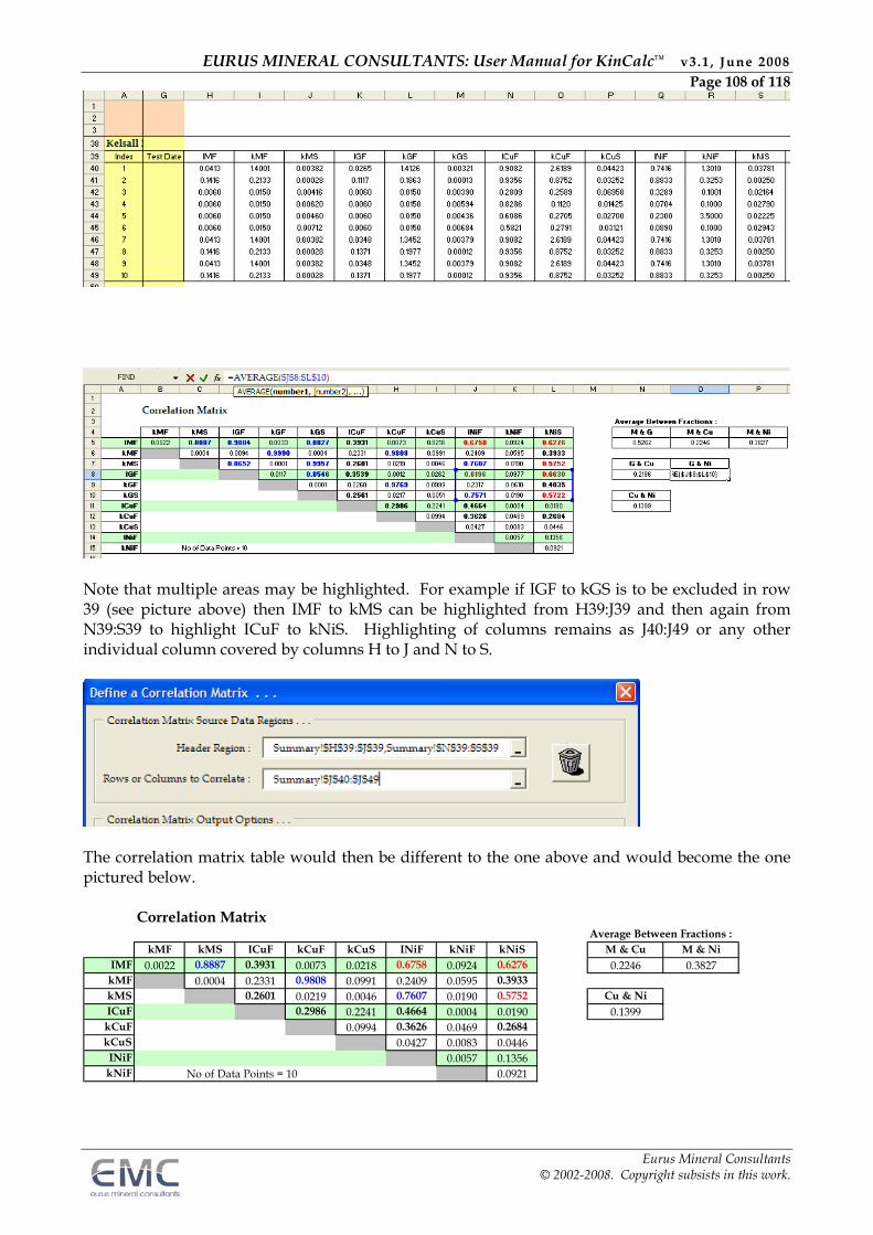
EURUS MINERAL CONSULTANTS: User Manual for KinCalc™ v3.1 , June 2008 Page 108 of 118
Eurus Mineral Consultants © 2002-2008. Copyright subsists in this work.
Note that multiple areas may be highlighted. For example if IGF to kGS is to be excluded in row 39 (see picture above) then IMF to kMS can be highlighted from H39:J39 and then again from N39:S39 to highlight ICuF to kNiS. Highlighting of columns remains as J40:J49 or any other individual column covered by columns H to J and N to S.
The correlation matrix table would then be different to the one above and would become the one pictured below.
Correlation MatrixAverage Between Fractions :
kMF kMS ICuF kCuF kCuS INiF kNiF kNiS M & Cu M & NiIMF 0.0022 0.8887 0.3931 0.0073 0.0218 0.6758 0.0924 0.6276 0.2246 0.3827kMF 0.0004 0.2331 0.9808 0.0991 0.2409 0.0595 0.3933kMS 0.2601 0.0219 0.0046 0.7607 0.0190 0.5752 Cu & NiICuF 0.2986 0.2241 0.4664 0.0004 0.0190 0.1399kCuF 0.0994 0.3626 0.0469 0.2684kCuS 0.0427 0.0083 0.0446INiF 0.0057 0.1356kNiF No of Data Points = 10 0.0921
EURUS MINERAL CONSULTANTS: User Manual for KinCalc™ v3.1 , June 2008 Page 109 of 118
Eurus Mineral Consultants © 2002-2008. Copyright subsists in this work.
Example The four tables below show correlation tables for rate tests on a base metal sulphide ore on samples of rougher feed, pulp down the rougher bank and rougher concentrate before and after regrinding. A column manually calculating the average for each kinetic parameter both across and down has been added. These values are tightly clustered around the overall average showing that, for fast and slow fraction and rate, there are no strong associations on a global basis when all components of floatable gangue and metal/mineral are taken into consideration. However, there are strong correlations on an individual basis such as;
Fast floating fractions and Gangue and Nickel (IGF vs INiF of r2 = 0.8780 ); top table, Fast and slow floating rates of Nickel and Cobalt (kNiF vs kCoF and kNiS vs kCoS of r2
= 0.8683 and 0.8637 respectively); top table, In the top two tables the averages for slow floating Gangue rate (kGS, highlighted at 0.085 and 0.136) are considerably less than the overall average and the spread of values for the rest of the kinetic parameters. This shows that mineral/gangue liberation in the slow floating component is good. The third table from the top details correlations for rate tests conducted on rougher concentrate. Here, the slow floating Gangue rate is on a par with the overall average because floatable Gangue has been defined as including Fe and S as well as silicate minerals. In this particular case Nickel and Cobalt occur in Pyrrhotite and Pentlandite which make-up the majority of floatable mass and relative to rougher feed these have been concentrated in the rougher concentrate stream. The purpose of regrinding is to improve liberation between mineral and Si and MgO bearing Gangue for subsequent smelting requirements. The bottom table details correlations for rate tests conducted on reground rougher concentrate. The effect of regrinding can be clearly seen from;
The average of slow floating Gangue rate (kGS) dropping from 0.224 to 0.159, The average of slow floating Nickel rate (kNiS) dropping from 0.213 to 0.076, The average between fractions dropping for Gangue/Nickel (0.2610 to 0.1969),
Gangue/Cobalt (0.2717 to 0.2110) and Nickel/Copper (0.3554 to 0.2650).
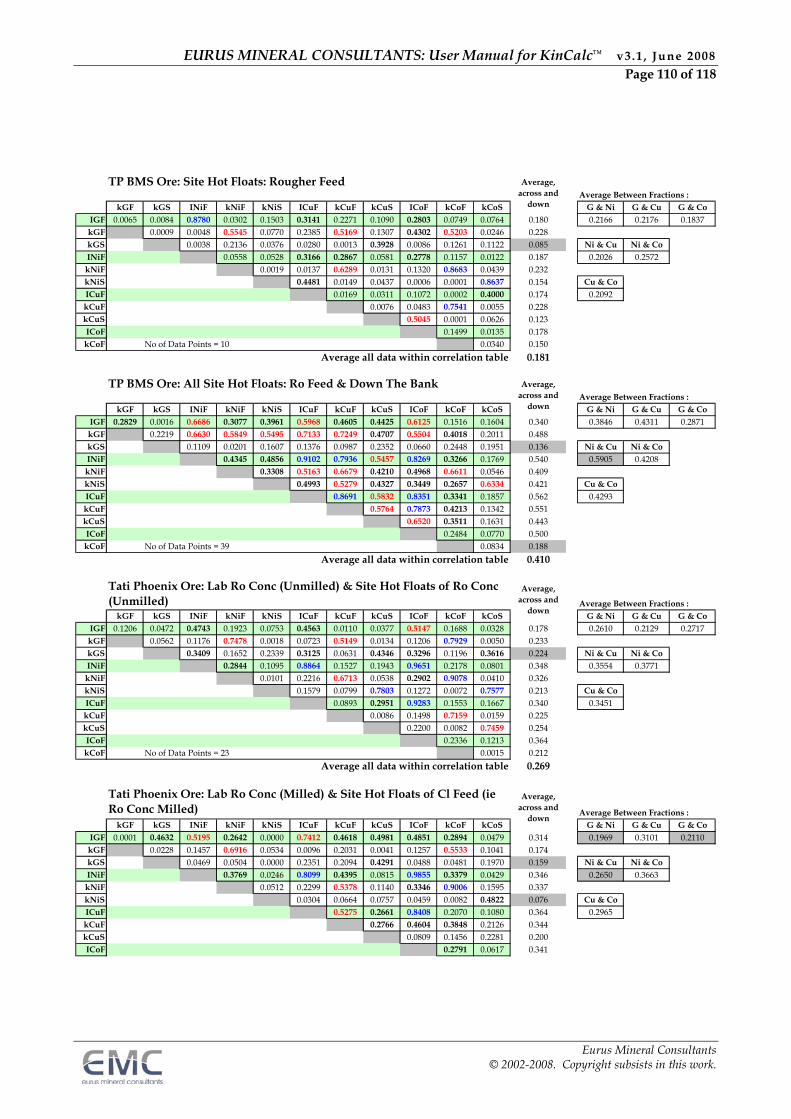
EURUS MINERAL CONSULTANTS: User Manual for KinCalc™ v3.1 , June 2008 Page 110 of 118
Eurus Mineral Consultants © 2002-2008. Copyright subsists in this work.
TP BMS Ore: Site Hot Floats: Rougher FeedAverage Between Fractions :
kGF kGS INiF kNiF kNiS ICuF kCuF kCuS ICoF kCoF kCoS G & Ni G & Cu G & CoIGF 0.0065 0.0084 0.8780 0.0302 0.1503 0.3141 0.2271 0.1090 0.2803 0.0749 0.0764 0.180 0.2166 0.2176 0.1837kGF 0.0009 0.0048 0.5545 0.0770 0.2385 0.5169 0.1307 0.4302 0.5203 0.0246 0.228kGS 0.0038 0.2136 0.0376 0.0280 0.0013 0.3928 0.0086 0.1261 0.1122 0.085 Ni & Cu Ni & CoINiF 0.0558 0.0528 0.3166 0.2867 0.0581 0.2778 0.1157 0.0122 0.187 0.2026 0.2572kNiF 0.0019 0.0137 0.6289 0.0131 0.1320 0.8683 0.0439 0.232kNiS 0.4481 0.0149 0.0437 0.0006 0.0001 0.8637 0.154 Cu & CoICuF 0.0169 0.0311 0.1072 0.0002 0.4000 0.174 0.2092kCuF 0.0076 0.0483 0.7541 0.0055 0.228kCuS 0.5045 0.0001 0.0626 0.123ICoF 0.1499 0.0135 0.178kCoF No of Data Points = 10 0.0340 0.150
Average all data within correlation table 0.181
TP BMS Ore: All Site Hot Floats: Ro Feed & Down The BankAverage Between Fractions :
kGF kGS INiF kNiF kNiS ICuF kCuF kCuS ICoF kCoF kCoS G & Ni G & Cu G & CoIGF 0.2829 0.0016 0.6686 0.3077 0.3961 0.5968 0.4605 0.4425 0.6125 0.1516 0.1604 0.340 0.3846 0.4311 0.2871kGF 0.2219 0.6630 0.5849 0.5495 0.7133 0.7249 0.4707 0.5504 0.4018 0.2011 0.488kGS 0.1109 0.0201 0.1607 0.1376 0.0987 0.2352 0.0660 0.2448 0.1951 0.136 Ni & Cu Ni & CoINiF 0.4345 0.4856 0.9102 0.7936 0.5457 0.8269 0.3266 0.1769 0.540 0.5905 0.4208kNiF 0.3308 0.5163 0.6679 0.4210 0.4968 0.6611 0.0546 0.409kNiS 0.4993 0.5279 0.4327 0.3449 0.2657 0.6334 0.421 Cu & CoICuF 0.8691 0.5832 0.8351 0.3341 0.1857 0.562 0.4293kCuF 0.5764 0.7873 0.4213 0.1342 0.551kCuS 0.6520 0.3511 0.1631 0.443ICoF 0.2484 0.0770 0.500kCoF No of Data Points = 39 0.0834 0.188
Average all data within correlation table 0.410
Average Between Fractions :kGF kGS INiF kNiF kNiS ICuF kCuF kCuS ICoF kCoF kCoS G & Ni G & Cu G & Co
IGF 0.1206 0.0472 0.4743 0.1923 0.0753 0.4563 0.0110 0.0377 0.5147 0.1688 0.0328 0.178 0.2610 0.2129 0.2717kGF 0.0562 0.1176 0.7478 0.0018 0.0723 0.5149 0.0134 0.1206 0.7929 0.0050 0.233kGS 0.3409 0.1652 0.2339 0.3125 0.0631 0.4346 0.3296 0.1196 0.3616 0.224 Ni & Cu Ni & CoINiF 0.2844 0.1095 0.8864 0.1527 0.1943 0.9651 0.2178 0.0801 0.348 0.3554 0.3771kNiF 0.0101 0.2216 0.6713 0.0538 0.2902 0.9078 0.0410 0.326kNiS 0.1579 0.0799 0.7803 0.1272 0.0072 0.7577 0.213 Cu & CoICuF 0.0893 0.2951 0.9283 0.1553 0.1667 0.340 0.3451kCuF 0.0086 0.1498 0.7159 0.0159 0.225kCuS 0.2200 0.0082 0.7459 0.254ICoF 0.2336 0.1213 0.364kCoF No of Data Points = 23 0.0015 0.212
Average all data within correlation table 0.269
Average Between Fractions :kGF kGS INiF kNiF kNiS ICuF kCuF kCuS ICoF kCoF kCoS G & Ni G & Cu G & Co
IGF 0.0001 0.4632 0.5195 0.2642 0.0000 0.7412 0.4618 0.4981 0.4851 0.2894 0.0479 0.314 0.1969 0.3101 0.2110kGF 0.0228 0.1457 0.6916 0.0534 0.0096 0.2031 0.0041 0.1257 0.5533 0.1041 0.174kGS 0.0469 0.0504 0.0000 0.2351 0.2094 0.4291 0.0488 0.0481 0.1970 0.159 Ni & Cu Ni & CoINiF 0.3769 0.0246 0.8099 0.4395 0.0815 0.9855 0.3379 0.0429 0.346 0.2650 0.3663kNiF 0.0512 0.2299 0.5378 0.1140 0.3346 0.9006 0.1595 0.337kNiS 0.0304 0.0664 0.0757 0.0459 0.0082 0.4822 0.076 Cu & CoICuF 0.5275 0.2661 0.8408 0.2070 0.1080 0.364 0.2965kCuF 0.2766 0.4604 0.3848 0.2126 0.344kCuS 0.0809 0.1456 0.2281 0.200ICoF 0.2791 0.0617 0.341
Average, across and
down
Tati Phoenix Ore: Lab Ro Conc (Unmilled) & Site Hot Floats of Ro Conc (Unmilled)
Average, across and
down
Tati Phoenix Ore: Lab Ro Conc (Milled) & Site Hot Floats of Cl Feed (ie Ro Conc Milled)
Average, across and
down
Average, across and
down
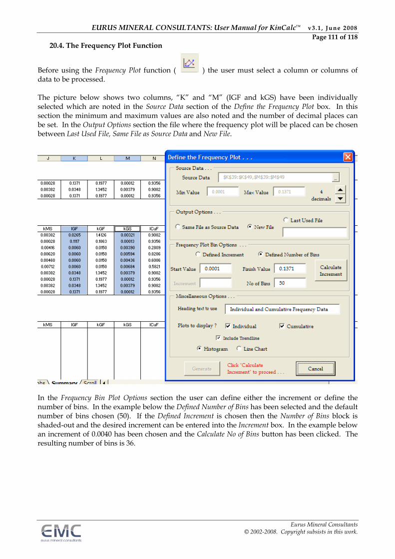
EURUS MINERAL CONSULTANTS: User Manual for KinCalc™ v3.1 , June 2008 Page 111 of 118
Eurus Mineral Consultants © 2002-2008. Copyright subsists in this work.
20.4. The Frequency Plot Function
Before using the Frequency Plot function ( ) the user must select a column or columns of data to be processed. The picture below shows two columns, “K” and “M” (IGF and kGS) have been individually selected which are noted in the Source Data section of the Define the Frequency Plot box. In this section the minimum and maximum values are also noted and the number of decimal places can be set. In the Output Options section the file where the frequency plot will be placed can be chosen between Last Used File, Same File as Source Data and New File.
In the Frequency Bin Plot Options section the user can define either the increment or define the number of bins. In the example below the Defined Number of Bins has been selected and the default number of bins chosen (50). If the Defined Increment is chosen then the Number of Bins block is shaded-out and the desired increment can be entered into the Increment box. In the example below an increment of 0.0040 has been chosen and the Calculate No of Bins button has been clicked. The resulting number of bins is 36.
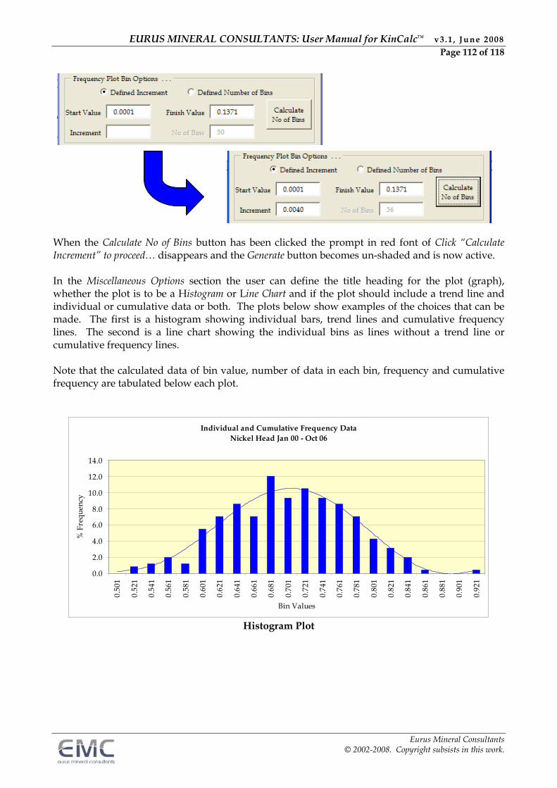
EURUS MINERAL CONSULTANTS: User Manual for KinCalc™ v3.1 , June 2008 Page 112 of 118
Eurus Mineral Consultants © 2002-2008. Copyright subsists in this work.
When the Calculate No of Bins button has been clicked the prompt in red font of Click “Calculate Increment” to proceed… disappears and the Generate button becomes un-shaded and is now active. In the Miscellaneous Options section the user can define the title heading for the plot (graph), whether the plot is to be a Histogram or Line Chart and if the plot should include a trend line and individual or cumulative data or both. The plots below show examples of the choices that can be made. The first is a histogram showing individual bars, trend lines and cumulative frequency lines. The second is a line chart showing the individual bins as lines without a trend line or cumulative frequency lines. Note that the calculated data of bin value, number of data in each bin, frequency and cumulative frequency are tabulated below each plot.
Individual and Cumulative Frequency DataNickel Head Jan 00 - Oct 06
0.0
2.0
4.0
6.0
8.0
10.0
12.0
14.0
0.50
1
0.52
1
0.54
1
0.56
1
0.58
1
0.60
1
0.62
1
0.64
1
0.66
1
0.68
1
0.70
1
0.72
1
0.74
1
0.76
1
0.78
1
0.80
1
0.82
1
0.84
1
0.86
1
0.88
1
0.90
1
0.92
1
Bin Values
% F
requ
ency
Histogram Plot
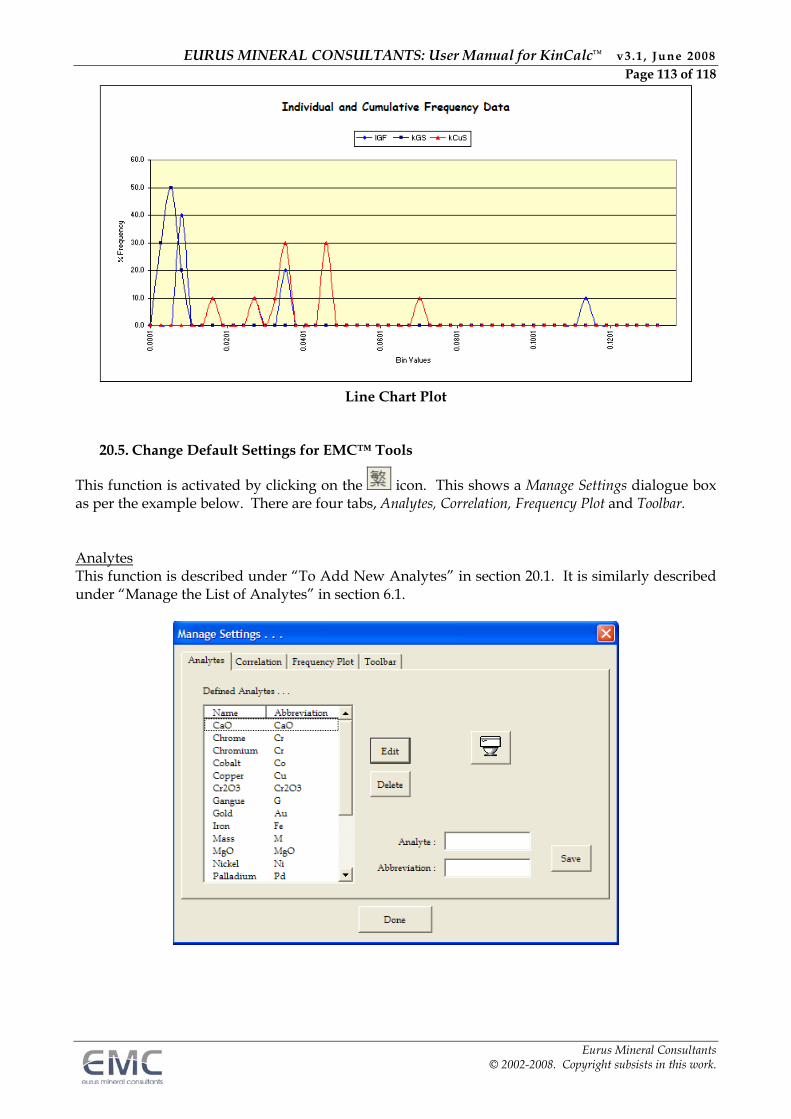
EURUS MINERAL CONSULTANTS: User Manual for KinCalc™ v3.1 , June 2008 Page 113 of 118
Eurus Mineral Consultants © 2002-2008. Copyright subsists in this work.
Line Chart Plot
20.5. Change Default Settings for EMC™ Tools
This function is activated by clicking on the icon. This shows a Manage Settings dialogue box as per the example below. There are four tabs, Analytes, Correlation, Frequency Plot and Toolbar.
Analytes This function is described under “To Add New Analytes” in section 20.1. It is similarly described under “Manage the List of Analytes” in section 6.1.
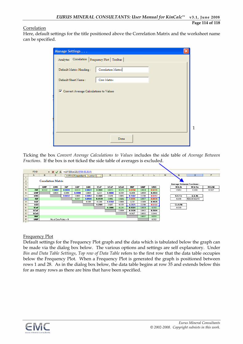
EURUS MINERAL CONSULTANTS: User Manual for KinCalc™ v3.1 , June 2008 Page 114 of 118
Eurus Mineral Consultants © 2002-2008. Copyright subsists in this work.
Correlation Here, default settings for the title positioned above the Correlation Matrix and the worksheet name can be specified.
Ticking the box Convert Average Calculations to Values includes the side table of Average Between Fractions. If the box is not ticked the side table of averages is excluded.
Frequency Plot Default settings for the Frequency Plot graph and the data which is tabulated below the graph can be made via the dialog box below. The various options and settings are self explanatory. Under Bin and Data Table Settings, Top row of Data Table refers to the first row that the data table occupies below the Frequency Plot. When a Frequency Plot is generated the graph is positioned between rows 1 and 28. As in the dialog box below, the data table begins at row 35 and extends below this for as many rows as there are bins that have been specified.
1
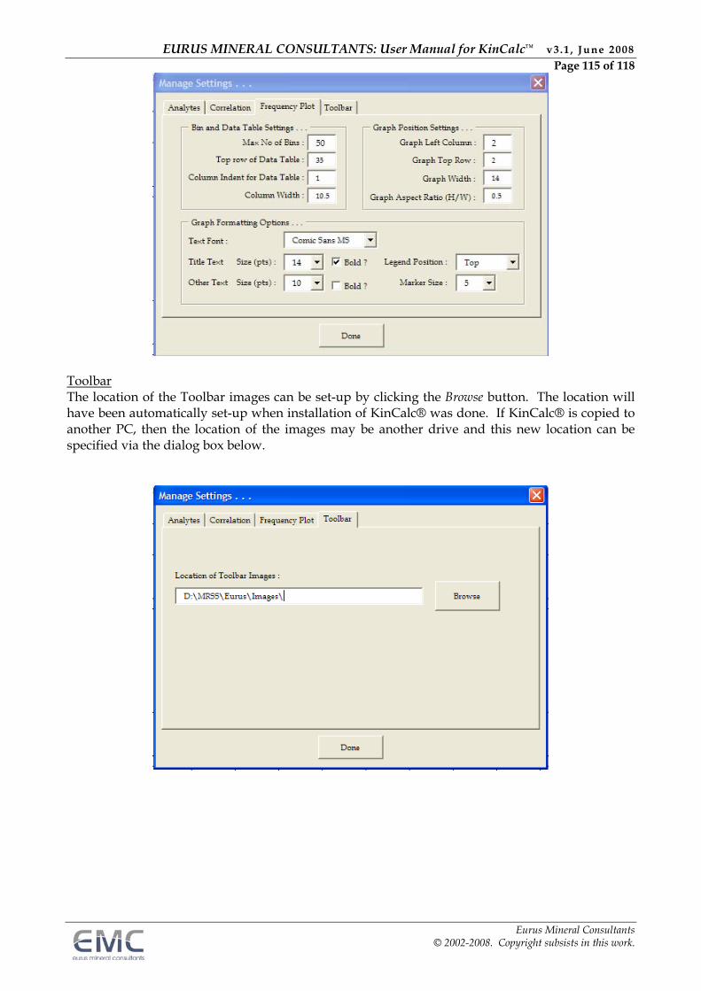
EURUS MINERAL CONSULTANTS: User Manual for KinCalc™ v3.1 , June 2008 Page 115 of 118
Eurus Mineral Consultants © 2002-2008. Copyright subsists in this work.
Toolbar The location of the Toolbar images can be set-up by clicking the Browse button. The location will have been automatically set-up when installation of KinCalc® was done. If KinCalc® is copied to another PC, then the location of the images may be another drive and this new location can be specified via the dialog box below.
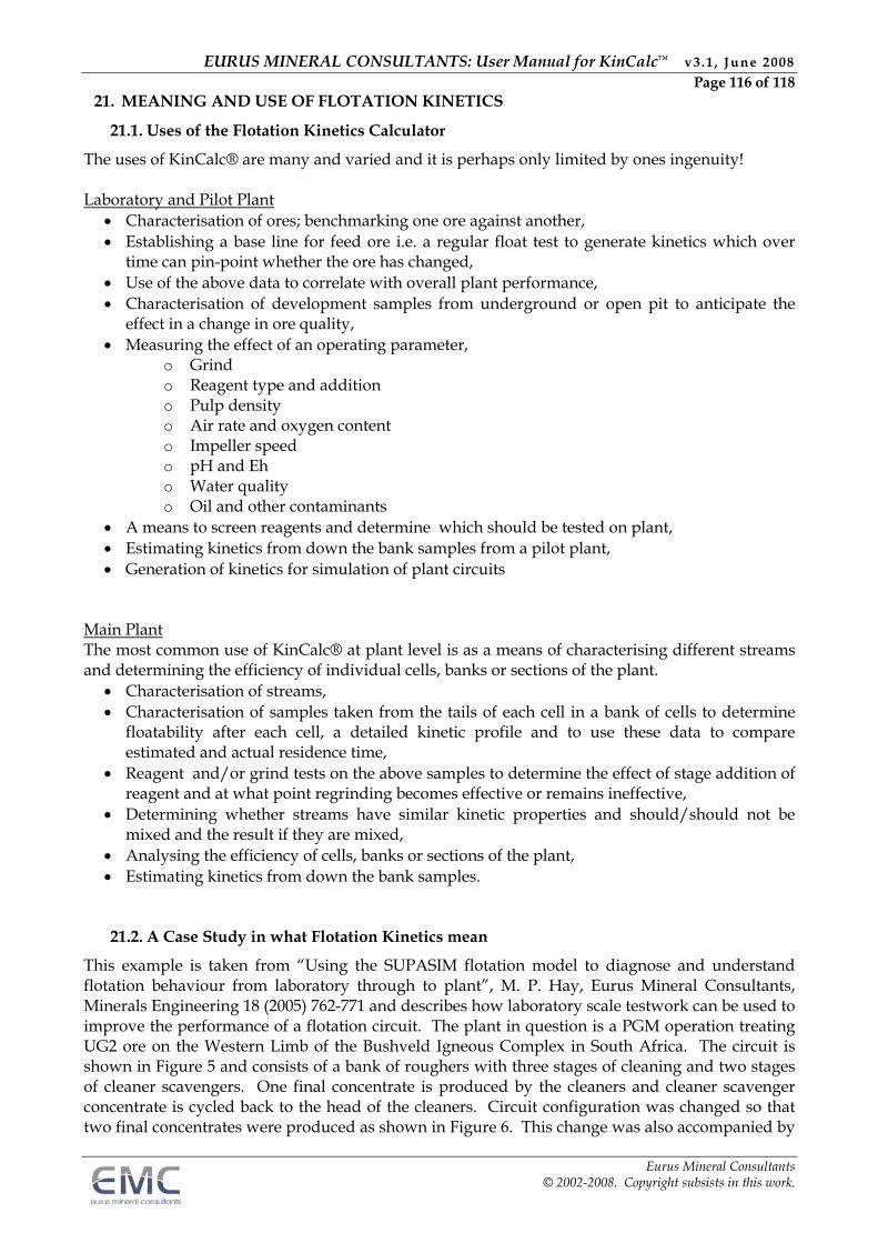
EURUS MINERAL CONSULTANTS: User Manual for KinCalc™ v3.1 , June 2008 Page 116 of 118
Eurus Mineral Consultants © 2002-2008. Copyright subsists in this work.
21. MEANING AND USE OF FLOTATION KINETICS
21.1. Uses of the Flotation Kinetics Calculator
The uses of KinCalc® are many and varied and it is perhaps only limited by ones ingenuity! Laboratory and Pilot Plant
Characterisation of ores; benchmarking one ore against another, Establishing a base line for feed ore i.e. a regular float test to generate kinetics which over
time can pin-point whether the ore has changed, Use of the above data to correlate with overall plant performance, Characterisation of development samples from underground or open pit to anticipate the
effect in a change in ore quality, Measuring the effect of an operating parameter,
o Grind o Reagent type and addition o Pulp density o Air rate and oxygen content o Impeller speed o pH and Eh o Water quality o Oil and other contaminants
A means to screen reagents and determine which should be tested on plant, Estimating kinetics from down the bank samples from a pilot plant, Generation of kinetics for simulation of plant circuits
Main Plant The most common use of KinCalc® at plant level is as a means of characterising different streams and determining the efficiency of individual cells, banks or sections of the plant.
Characterisation of streams, Characterisation of samples taken from the tails of each cell in a bank of cells to determine
floatability after each cell, a detailed kinetic profile and to use these data to compare estimated and actual residence time,
Reagent and/or grind tests on the above samples to determine the effect of stage addition of reagent and at what point regrinding becomes effective or remains ineffective,
Determining whether streams have similar kinetic properties and should/should not be mixed and the result if they are mixed,
Analysing the efficiency of cells, banks or sections of the plant, Estimating kinetics from down the bank samples.
21.2. A Case Study in what Flotation Kinetics mean
This example is taken from “Using the SUPASIM flotation model to diagnose and understand flotation behaviour from laboratory through to plant”, M. P. Hay, Eurus Mineral Consultants, Minerals Engineering 18 (2005) 762-771 and describes how laboratory scale testwork can be used to improve the performance of a flotation circuit. The plant in question is a PGM operation treating UG2 ore on the Western Limb of the Bushveld Igneous Complex in South Africa. The circuit is shown in Figure 5 and consists of a bank of roughers with three stages of cleaning and two stages of cleaner scavengers. One final concentrate is produced by the cleaners and cleaner scavenger concentrate is cycled back to the head of the cleaners. Circuit configuration was changed so that two final concentrates were produced as shown in Figure 6. This change was also accompanied by
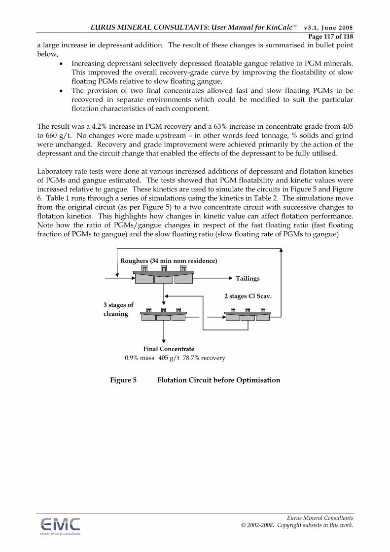
EURUS MINERAL CONSULTANTS: User Manual for KinCalc™ v3.1 , June 2008 Page 117 of 118
Eurus Mineral Consultants © 2002-2008. Copyright subsists in this work.
a large increase in depressant addition. The result of these changes is summarised in bullet point below,
Increasing depressant selectively depressed floatable gangue relative to PGM minerals. This improved the overall recovery-grade curve by improving the floatability of slow floating PGMs relative to slow floating gangue,
The provision of two final concentrates allowed fast and slow floating PGMs to be recovered in separate environments which could be modified to suit the particular flotation characteristics of each component.
The result was a 4.2% increase in PGM recovery and a 63% increase in concentrate grade from 405 to 660 g/t. No changes were made upstream – in other words feed tonnage, % solids and grind were unchanged. Recovery and grade improvement were achieved primarily by the action of the depressant and the circuit change that enabled the effects of the depressant to be fully utilised. Laboratory rate tests were done at various increased additions of depressant and flotation kinetics of PGMs and gangue estimated. The tests showed that PGM floatability and kinetic values were increased relative to gangue. These kinetics are used to simulate the circuits in Figure 5 and Figure 6. Table 1 runs through a series of simulations using the kinetics in Table 2. The simulations move from the original circuit (as per Figure 5) to a two concentrate circuit with successive changes to flotation kinetics. This highlights how changes in kinetic value can affect flotation performance. Note how the ratio of PGMs/gangue changes in respect of the fast floating ratio (fast floating fraction of PGMs to gangue) and the slow floating ratio (slow floating rate of PGMs to gangue).
Roughers (34 min nom residence)
Tailings
2 stages Cl Scav.3 stages ofcleaning
Final Concentrate0.9% mass 405 g/t 78.7% recovery
Figure 5 Flotation Circuit before Optimisation
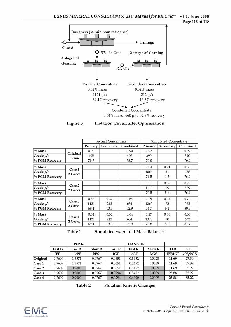
EURUS MINERAL CONSULTANTS: User Manual for KinCalc™ v3.1 , June 2008 Page 118 of 118
Eurus Mineral Consultants © 2002-2008. Copyright subsists in this work.
Roughers (34 min nom residence)
TailingsRT:feed
RT: Ro Conc 2 stages of cleaning 3 stages ofcleaning
Primary Concentrate Secondary Concentrate0.32% mass 0.32% mass
1121 g/t 212 g/t69.4% recovery 13.5% recovery
Combined Concentrate0.64% mass 660 g/t 82.9% recovery
RT: Cl T
Figure 6 Flotation Circuit after Optimisation
Primary Secondary Combined Primary Secondary Combined% Mass 0.90 0.90 0.92 0.92Grade g/t 405 405 390 390% PGM Recovery 78.7 78.7 76.0 76.0
% Mass 0.34 0.24 0.58Grade g/t 1064 31 638% PGM Recovery 74.5 1.5 76.0
% Mass 0.31 0.39 0.70Grade g/t 1113 69 529% PGM Recovery 70.5 5.6 76.1
% Mass 0.32 0.32 0.64 0.29 0.41 0.70Grade g/t 1121 212 631 1265 73 562% PGM Recovery 69.4 13.5 82.9 74.7 6.1 80.8
% Mass 0.32 0.32 0.64 0.27 0.36 0.63Grade g/t 1121 212 631 1378 80 632% PGM Recovery 69.4 13.5 82.9 75.8 5.9 81.7
Case 2 2 Concs
Case 3 2 Concs
Case 4 2 Concs
Actual Concentrate Simulated Concentrate
Original 1 Conc
Case 1 2 Concs
Table 1 Simulated vs. Actual Mass Balances
Fast Fr. Fast R. Slow R. Fast Fr. Fast R. Slow R. FFR SFR IPF kPF kPS IGF kGF kGS IPF/IGF kPS/kGS
Original 0.7609 1.3571 0.0767 0.0651 0.5452 0.0028 11.69 27.39Case 1 0.7609 1.3571 0.0767 0.0651 0.5452 0.0028 11.69 27.39Case 2 0.7609 0.9000 0.0767 0.0651 0.5452 0.0009 11.69 85.22Case 3 0.7609 0.9000 0.0767 0.0294 0.5452 0.0009 25.88 85.22Case 4 0.7609 0.9000 0.0767 0.0294 0.4000 0.0009 25.88 85.22
PGMs GANGUE
Table 2 Flotation Kinetic Changes