Floristic units and their predictors unveiled in part of … 4930, Jardim Flamboyant, 78580-000 Alta Floresta, MT, Brasil 3Instituto Federal de Educação, Ciência e Tecnologia do

An Acad Bras Cienc (2015) 87 (4)

Anais da Academia Brasileira de Ciências (2015) 87(4): 2031-2046(Annals of the Brazilian Academy of Sciences)Printed version ISSN 0001-3765 / Online version ISSN 1678-2690http://dx.doi.org/10.1590/0001-3765201520140132www.scielo.br/aabc

Floristic units and their predictors unveiled in part of the Atlantic Forest hotspot: implications for conservation planning

FELIPE z. SAITER¹, PEDRO v. EISENLOhR², GLAUCO S. FRANçA³, JOãO R. STEhMANN4, WILLIAM W. ThOMAS5 and ARY T. DE OLIvEIRA-FILhO4

1Instituto Federal de Educação, Ciência e Tecnologia do Espírito Santo, Campus Santa Teresa, Rodovia ES-080, Km 93, São João de Petrópolis, 29660-000 Santa Teresa, ES, Brasil

2Universidade do Estado de Mato Grosso, Campus Alta Floresta, Avenida Perimetral Rogério Silva, 4930, Jardim Flamboyant, 78580-000 Alta Floresta, MT, Brasil

3Instituto Federal de Educação, Ciência e Tecnologia do Sudeste de Minas Gerais, Campus Barbacena, Rua Monsenhor José Augusto, 204, São José, 36205-018 Barbacena, MG, Brasil

4Departamento de Botânica, Instituto de Ciências Biológicas, Universidade Federal de Minas Gerais, Avenida Antônio Carlos, 6627, Pampulha, 31270-110 Belo Horizonte, MG, Brasil

5The New York Botanical Garden, 2900 Southern Boulevard, 10458-5126, Bronx, NY, United States of America

Manuscript received on March 20, 2014; accepted for publication on January 19, 2015

ABSTRACTWe submitted tree species occurrence and geoclimatic data from 59 sites in a river basin in the Atlantic Forest of southeastern Brazil to ordination, ANOVA, and cluster analyses with the goals of investigating the causes of phytogeographic patterns and determining whether the six recognized subregions represent distinct floristic units. We found that both climate and space were significantly (p ≤ 0.05) important in the explanation of phytogeographic patterns. Floristic variations follow thermal gradients linked to elevation in both coastal and inland subregions. A gradient of precipitation seasonality was found to be related to floristic variation up to 100 km inland from the ocean. The temperature of the warmest quarter and the precipitation during the coldest quarter were the main predictors. The subregions Sandy Coastal Plain, Coastal Lowland, Coastal Highland, and Central Depression were recognized as distinct floristic units. Significant differences were not found between the Inland Highland and the Espinhaço Range, indicating that these subregions should compose a single floristic unit encompassing all interior highlands. Because of their ecological peculiarities, the ferric outcrops within the Espinhaço Range may constitute a special unit. The floristic units proposed here will provide important information for wiser conservation planning in the Atlantic Forest hotspot.Key words: Phytogeographic patterns, environmental gradients, spatial autocorrelation, Doce River basin.

Correspondence to: Felipe Zamborlini Saiter E-mail: [email protected]

INTRODUCTION

The patterns of geographic distribution of plant taxa are directed by a complex set of variables and interrelationships (Rizzini 1997). Among these, climatic variables deserve to be highlighted

in mesoscale approaches because, in several studies, they are indicated as the main predictors of phytogeographic patterns (e.g., Engelbrecht et al. 2007, Oliveira-Filho et al. 2005, Scudeller et al. 2001).

Climatic variables, especially those related to temperature and precipitation, are important because they directly influence plant development


2032 FELIPE Z. SAITER et al.

and are responsible for floristic changes along gradients (Grubb 1977, Pausas and Austin 2001). Precipitation gradients are quite complex and are influenced by factors such as surface roughness, distance to large water sources (oceans, inland seas and lakes) and air mass features (Wulf et al. 2010). The equally complex temperature gradients are linked to latitudinal changes in solar radiation (Breckle 2002, Kessler et al. 2011) and altitudinal changes in air pressure, humidity, and cloud cover (Körner 2007, Homeier et al. 2010).

Geographic location is also a relevant factor in floristic relationships among sites because floristic similarity is likely to increase with the spatial proximity (e.g., Scudeller et al. 2001, Oliveira-Filho et al. 2005, White and Hood 2004). Because of this, recent studies (e.g., Chain-Guadarrama et al. 2012, Gasper et al. 2013) have added spatial filters in statistical analyses to minimize the effect of spatial autocorrelation on the interpretation of the relationship among species distributions and environmental variables (Eisenlohr 2013, Legendre and Legendre 2012, Zimmermann et al. 2010).

In the Atlantic Forest of southeastern Brazil, a region with high diversity and endemism (França and Stehmann 2013, Rolim et al. 2006, Saiter et al. 2011), phytogeographic studies indicate that changes in tree composition are related to at least three major climatic gradients: a coastal-inland gradient of precipitation seasonality (Oliveira-Filho and Fontes 2000, Oliveira-Filho et al. 2005, Santos et al. 2011), a latitudinal gradient of temperature (Oliveira-Filho and Fontes 2000, Oliveira-Filho et al. 2005), and an altitudinal gradient of temperature and humidity (Torres et al. 1997, Oliveira-Filho and Fontes 2000, Oliveira-Filho et al. 2005, Bertoncello et al. 2011, Kamino et al. 2008). Such phytogeographic patterns, however, are generalizations for a large and environmentally complex region (see Oliveira-Filho et al. 2005) and it is possible that they do not accurately explain the floristic variation in finer mesoscales.

Understanding subregional floristic patterns is still a challenge to elucidate the phytogeography of southeastern Brazil, taking into account that the Brazilian flora, as a whole, remains undercollected (Sobral and Stehmann 2009). Furthermore, policies for forest conservation, such as those related to the creation of parks and reserves, restoration of ecosystems, and sustainable use of natural products, can be more appropriately planned when biological-environmental changes throughout the region are better known (McShea et al. 2014).

Within southeastern Brazil, the Doce River Basin (DRB) is an interesting region for investigating subregional phytogeographic patterns because of its high number of forest inventories and botanical collections. The DRB also shows high environmental heterogeneity, with three coastal subregions (Sandy Coastal Plain, Coastal Lowland, and Coastal Highland) and three inland subregions (Central Depression, Interior Highland, and Espinhaço Range) recognized through geomorphology and climatic features (Cupolillo et al. 2008, Instituto Mineiro de Gestão das Águas 2010, Nascimento et al. 2012).

Our goals were to answer the following questions using floristic and geoclimatic data: [1] Which climatic variables better explain subregional phytogeographic patterns in the DRB? [2] Does spatial proximity among sites influence these patterns? [3] Do the subregions of the DRB deserve to be treated as distinct floristic units? We addressed such questions considering, in particular, the implications for biological conservation in the Atlantic Forest hotspot.

MATERIALS AND METhODS

study area

The Doce River Basin (DRB) encompasses approximately 87,000 km2 in the eastern region of the state of Minas Gerais and the central and northern portions of the state of Espírito Santo in


FLORISTIC UNITS IN THE ATLANTIC FOREST 2033

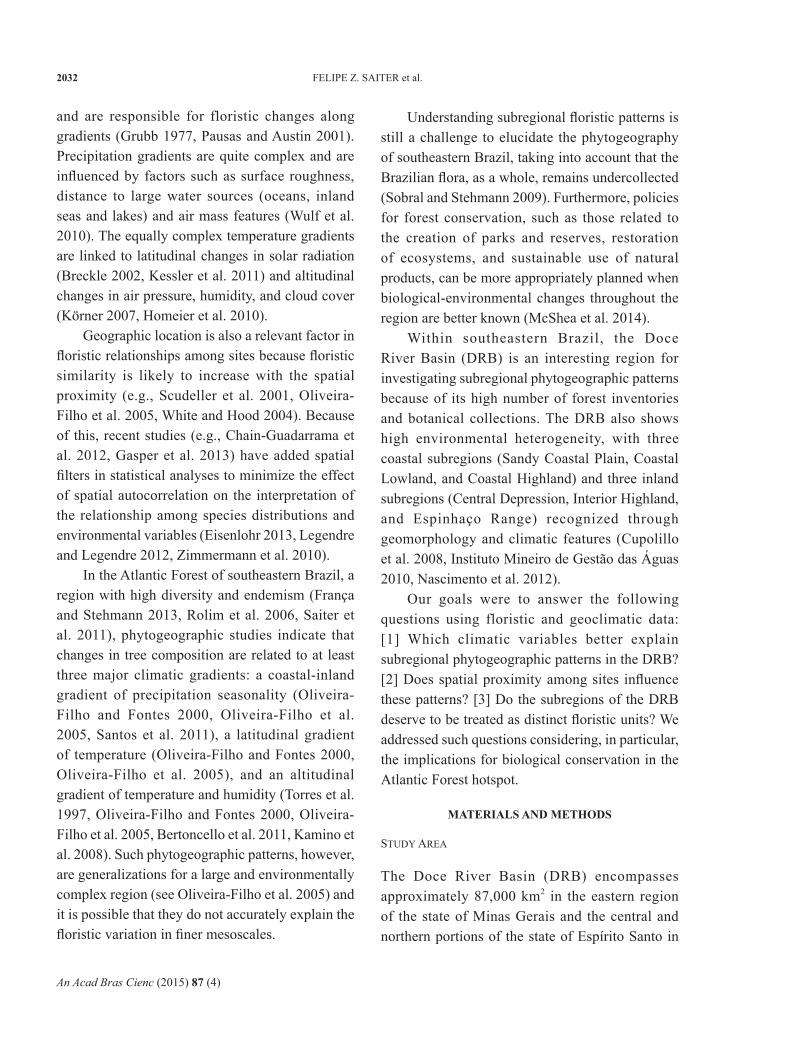
southeastern Brazil (Instituto Mineiro de Gestão das Águas 2010). The DRB is limited to the north by the Negra and Aimorés Mountains, to the west by the Espinhaço Range, to the southwest by the Mantiqueira Range, to the southeast by the Caparaó Range, and to the east by the Atlantic Ocean (Instituto Mineiro de Gestão das Águas 2010; Fig. 1). We added the small Barra Seca River Basin to the final stretch of the DRB in order to include Sandy Coastal Plain and Lowland sites of northern Espírito Santo into the dataset.

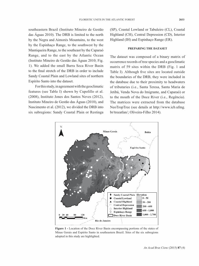
For this study, in agreement with the geoclimatic features (see Table I) shown by Cupolillo et al. (2008), Instituto Jones dos Santos Neves (2012), Instituto Mineiro de Gestão das Águas (2010), and Nascimento et al. (2012), we divided the DRB into six subregions: Sandy Coastal Plain or Restinga

(SP), Coastal Lowland or Tabuleiro (CL), Coastal Highland (CH), Central Depression (CD), Interior Highland (IH) and Espinhaço Range (ER).

PREPARING ThE DATASET

The dataset was composed of a binary matrix of occurrence records of tree species and a geoclimatic matrix of 59 sites within the DRB (Fig. 1 and Table I). Although five sites are located outside the boundaries of the DRB, they were included in the database due to their proximity to headwaters of tributaries (i.e., Santa Teresa, Santa Maria de Jetibá, Venda Nova do Imigrante, and Caparaó) or to the mouth of the Doce River (i.e., Regência). The matrices were extracted from the database NeoTropTree (see details at http://www.icb.ufmg.br/treeatlan/; Oliveira-Filho 2014).

Figure 1 - Location of the Doce River Basin encompassing portions of the states of Minas Gerais and Espírito Santo in southeastern Brazil. Sites of the six subregions adopted in this study are highlighted.



TAB

LE

I Si

tes a

nd g

ener

al c

hara

cter

istic

s of s

ix su

breg

ions

with

in th

e D

oce

Riv

er B

asin

, sou

thea

ster

n B

razi

l. AT

, A

nnua

l mea

n te

mpe

ratu

re; A

P, A

nnua

l mea

n pr

ecip

itatio

n.

Subr

egio

nSi

tes

AT (°

C)

AP

(mm

/yr)

Ele

vatio

n (m

)G

eom

orph

olog

y

Sand

y C

oast

al

Plai

nE

Slir

s (D

egre

do),

ESp

tip (P

onta

l do

Ipira

nga)

, ESr

ege

(Reg

ênci

a)24

1,20

0-1,

300

0-50

Plai

ns fo

rmed

by

sand

y se

dim

ents

fr

om Q

uate

rnar

y

Coa

stal

Low

land

ESl

inh

(Lin

hare

s), E

Sflon

(FLO

NA

Goy

taca

zes)

, ESs

oor

(Soo

reta

ma)

24 1

,200

-1,2

50<

200

Flat

tene

d lo

amy-

sand

y se

dim

ents

(B

arre

iras G

roup

) fro

m T

ertia

ry

Coa

stal

Hig

hlan

dE

Sjtb

a (S

anta

Mar

ia d

e Je

tibá)

, ESs

ant (

Sant

a Ter

esa)

, ESv

nim

(Ven

da

Nov

a do

Imig

rant

e), M

Gar

ap (A

rapo

nga)

, MG

capa

(Cap

araó

)18

-21

1,30

0-1,

800

600-

2,00

0D

isse

cted

Pre

cam

bria

n pl

atea

us

Cen

tral

Dep

ress

ion

ESa

gbr

(Águ

ia B

ranc

a), E

Salib

(A

lto L

iber

dade

), E

Scol

a (C

olat

ina)

, E

Sita

g (I

tagu

açu)

, ESp

alh

(São

Gab

riel d

a Pa

lha)

, ESp

anc

(Pan

cas)

, E

Ssjp

t (S

ão

João

de

Pe

trópo

lis),

MG

aim

o (A

imor

és),

MG

anto

(A

ntôn

io D

ias)

, MG

baix

(São

Ger

aldo

do

Bai

xio)

, MG

brau

(Bra

únas

), M

Gca

rt (C

arat

inga

), M

Gdi

on (D

ioní

sio)

, MG

ipan

(Ipa

nem

a), M

Gip

at

(Ipa

tinga

), M

Gita

m (

Itam

bé d

o M

ato

Den

tro),

MG

gove

(G

over

nado

r Va

lada

res)

, M

Ggu

ar

(Gua

raci

aba)

, M

Gip

ab

(Ipa

ba),

MG

mrl

c (M

arila

c),

MG

mar

l (M

arlié

ria),

MG

ping

(Pi

ngo

d’Á

gua)

, M

Gpo

nt

(Pon

te N

ova)

, M

Gpt

qm (

Pont

e Q

ueim

ada)

, M

Grd

oc (

Rio

Doc

e),

MG

silv

(La

goa

Silv

ano)

, MG

sped

(Sã

o Pe

dro

do S

uaçu

í), M

Gtim

o (T

imót

eo),

MG

vinh

(Vin

hátic

o)

24-2

51,

000-

1,20

0<

600

Hill

s and

fluv

ial p

lain

s with

dee

p so

ils w

ithin

a in

ter-p

late

aus z

one

Inte

rior H

ighl

and

MG

diog

(D

iogo

de

Vasc

once

los)

, M

Gev

an (

São

João

Eva

ngel

ista

), M

Gm

ari

(Mar

iana

), M

Gm

onl

(Joã

o M

onle

vade

), M

Gpe

na

(Con

selh

eiro

Pen

a),

MG

pinh

(Pi

nhei

ro A

lto),

MG

pira

(Pi

rang

a),

MG

rver

(R

io V

erm

elho

), M

Gsg

ra (

São

Gon

çalo

do

Rio

Aba

ixo)

, M

Gvi

co (V

iços

a)

19-2

11,

200-

1,40

060

0-1,

000

Dis

sect

ed P

reca

mbr

ian

plat

eaus

Espi

nhaç

o R

ange

MG

cboi

(Cab

eça

de B

oi),

MG

cata

(Cat

as A

ltas d

a N

orue

ga),

MG

mtd

r (C

once

ição

do

Mat

o D

entro

), M

Gpi

la (

Mor

ro d

o Pi

lar)

, M

Gca

ra

(San

tuár

io d

o C

araç

a), M

Gri

oa (S

erra

da

Gan

dare

la),

MG

sam

b (S

erra

do

Am

brós

io),

MG

serr

(Ser

ro),

MG

opnn

(Our

o Pr

eto)

18-2

01,

400-

1,80

01,

000-

1,60

0

Peak

s, rid

ges a

nd e

scar

pmen

ts

of q

uartz

ic o

r fer

ric ro

cks

from

Pre

cam

bria

n (B

razi

lian

Cry

stal

line

Shie

ld)



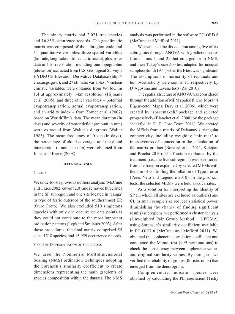
The binary matrix had 2,021 tree species and 16,835 occurrence records. The geoclimatic matrix was composed of the subregion code and 31 quantitative variables: three spatial variables (latitude, longitude and distance to ocean), plus raster data at 1-km resolution including one topographic (elevation) extracted from U.S. Geological Survey’s HYDRO1k Elevation Derivative Database (http://eros.usgs.gov/), and 27 climatic variables. Nineteen climatic variables were obtained from WorldClim 1.4 at approximately 1-km resolution (Hijmans et al. 2005), and three other variables – potential evapotranspiration, actual evapotranspiration, and an aridity index – from Zomer et al. (2007) based on WorldClim’s data. The mean duration (in days) and severity of water deficit (amount in mm) were extracted from Walter’s diagrams (Walter 1985). The mean frequency of frosts (in days), the percentage of cloud coverage, and the cloud interception (amount in mm) were obtained from Jones and Harris (2008).

DATA ANALYSES

Presets

We undertook a previous outliers analysis (McCune and Grace 2002; cut-off 2.0) and removed three sites in the SP subregion and one site located in ‘canga’ (a type of ferric outcrop) of the southernmost ER (Ouro Preto). We also excluded 510 singletons (species with only one occurrence data point) as they could not contribute to the most important ordination patterns (Lepš and Šmilauer 2003). After these procedures, the final matrix comprised 55 sites, 1518 species, and 15,959 occurrence records.

FLoristiC diFFerentiation oF suBregions

We used the Nonmetric Multidimensional Scaling (NMS) ordination techniques adopting the Sørensen’s similarity coefficient to create dimensions representing the main gradients of species composition within the dataset. The NMS

analysis was performed in the software PC-ORD 6 (McCune and Mefford 2011).

We evaluated the dissociation among five of six subregions through ANOVA with gradients scores (dimensions 1 and 2) that emerged from NMS, and then Tukey’s post hoc test adapted for unequal samples (Smith 1971) when the F test was significant. The assumptions of normality of residuals and homoscedasticity were confirmed, respectively, by D’Agostino and Levene tests (Zar 2010).

The spatial structure of ANOVA was considered through the addition of MEM spatial filters (Moran’s Eigenvector Maps; Dray et al. 2006), which were created by ‘spacemakeR’ package and selected progressively (Blanchet et al. 2008) by the package ‘packfor’ in R (R Core Team 2011). We created the MEMs from a matrix of Delaunay’s triangular connectivity, including weighing ‘min-max’ to intensiveness of connection in the calculation of the matrix-product (Borcard et al. 2011, Kelejian and Prucha 2010). The fraction explained by the treatment (i.e., the five subregions) was partitioned from the fraction explained by selected MEMs with the aim of controlling the inflation of Type I error (Peres-Neto and Legendre 2010). In the post hoc tests, the selected MEMs were held as covariates.

As a solution for interpreting the identity of SP (in which all sites are excluded as outliers) and CL (a small sample size reduced statistical power, diminishing the chance of finding significant results) subregions, we performed a cluster analysis (Unweighted Pair Group Method – UPGMA) using Sørensen’s similarity coefficient available in PC-ORD 6 (McCune and Mefford 2011). We obtained the cophenetic correlation coefficient and conducted the Mantel test (999 permutations) to check the consistency between cophenetic values and original similarity values. By doing so, we verified the reliability of groups (floristic units) that emerged from the dendrogram.

Complementary, indicator species were obtained by calculating the Phi coefficient (Tichý



and Chytrý 2006) in each floristic unit using the PC-ORD 6.0 software (McCune and Mefford 2011). The significance of Phi coefficient was tested using 999 Monte Carlo permutations. In order to obtain a set of the most representative indicator species, we selected only those with Phi coefficient ≥ 0.95 and/or p ≤ 0.001.

CorreLations aMong FLoristiCs and geoCLiMatiC variaBLes

We undertook correlations a posteriori among NMS dimensions and geoclimatic variables using Pearson’s correlation and linear regression models (OLS). Here we did not use latitude and longitude, since their influence on floristic gradients was checked through Moran’s correlograms (see below). We pre-selected some variables that showed clear relationships with floristic patterns in each dimension (visual analysis), and then eliminated co-linearities, excluding redundant variables with lower explanatory power. We considered the existence of co-linearity when the variance inflation factor (VIF) of each variable was greater than 10 (e.g., Quinn and Keough 2002). Then, we selected the models adopting the best balance between parsimony and accuracy of data description (i.e., lower AICc – corrected Akaike Information Criteria – value; Burnham and Anderson 2002). We confirmed the models’ assumptions considering the cautions indicated by Eisenlohr (2013). Specifically for normality of residuals, we used the D’Agostino-Pearson test (Zar 2010). Since we detected the absence of normality in models, we excluded outliers identified among studentized residuals (values > 2).

To evaluate gradients of species composition as a function of geographical distance, we verified the spatial structure of scores of each significant dimension of NMS through correlograms created by the software SAM 4.0 (Rangel et al. 2010) adopting Moran’s I coefficient (Legendre and

Fortin 1989) and following the default options. We tested the global significance of correlograms using Bonferroni’s sequential correction, and confirmed the existence of spatial structure when at least one distance class was significant (Fortin and Dale 2005).

Since spatial structure in both response variables and predictors can inflate the Type I error (Peres-Neto and Legendre 2010), we also prepared correlograms for each individual variable, regardless of the residuals independence assumption (Landeiro and Magnusson 2011). Because we found spatial structure in all variables, we also prepared spatially explicit models to confirm the significances found. We also prepared partitioned models in the same manner as described above. Because the significance of these models was supported, we opted to show the results of the simplest models, i.e., without inclusion of MEMs.

varianCe Partitioning

Following the protocol suggested by Eisenlohr (2014), we performed a variance partitioning of the explanation provided by: [a] only climatic variables + elevation, [b] the spatially structured fraction of these variables, [c] only spatial components, and [d] factors not measured. Here we used the packages ‘vegan’, ‘spacemakeR’, ‘packfor’ and ‘spdep’ in R (R Core Team 2011).

To achieve this goal, the occurrence data were Hellinger transformed (Legendre and Gallagher 2001) and the MEMs were forward selected. We then processed two Canonical Redundance Analyses (RDA), the first involving species and environment, and the second involving environment and space (MEMs). Note that the variance partitioning makes the removal of co-linear variables unnecessary (Oksanen et al. 2013). We also tested the significance of pure fractions [a] and [c] by permutation-based ANOVA.



RESULTS

FLoristiC diFFerentiation oF suBregions

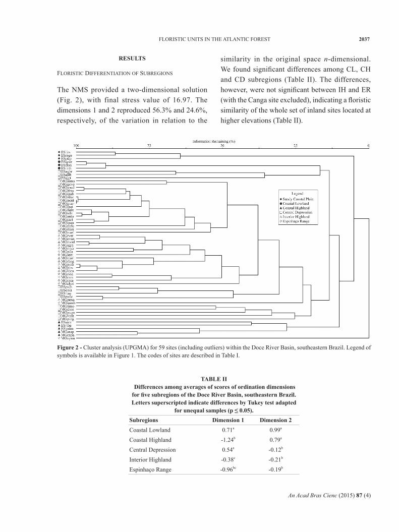
The NMS provided a two-dimensional solution (Fig. 2), with final stress value of 16.97. The dimensions 1 and 2 reproduced 56.3% and 24.6%, respectively, of the variation in relation to the

similarity in the original space n-dimensional. We found significant differences among CL, CH and CD subregions (Table II). The differences, however, were not significant between IH and ER (with the Canga site excluded), indicating a floristic similarity of the whole set of inland sites located at higher elevations (Table II).

TABLE II Differences among averages of scores of ordination dimensions for five subregions of the Doce River Basin, southeastern Brazil. Letters superscripted indicate differences by Tukey test adapted

for unequal samples (p ≤ 0.05).Subregions Dimension 1 Dimension 2Coastal Lowland 0.71a 0.99a

Coastal Highland -1.24b 0.79a

Central Depression 0.54a -0.12b

Interior Highland -0.38c -0.21b

Espinhaço Range -0.96bc -0.19b

Figure 2 - Cluster analysis (UPGMA) for 59 sites (including outliers) within the Doce River Basin, southeastern Brazil. Legend of symbols is available in Figure 1. The codes of sites are described in Table I.



The floristic identity of IH plus ER was confirmed by UPGMA (Fig. 2; cophenetic correlation coefficient = 0.90; Mantel bi-lateral test, p = 0.001), because sites of IH and ER were integrated in the same group (with the exception of the Conselheiro Pena and Serra do Ambrósio sites), in the middle portion of the dendrogram. The UPGMA also confirmed the floristic identity of the SP subregion and CL subregion through the emergence of discrete groups (floristic units). The Canga site of the southernmost ER constituted a floristic unit separated from other localities in the Espinhaço Range. Indicator species of six floristic units (i.e., SP, CL, CH, CD, IH plus ER, and Canga) emerged from the analyses and are listed in Table IV. Such indicator species are the most frequent and exclusive species in each floristic unit.

CorreLations aMong FLoristiC CoMPosition and geoCLiMatiC variaBLes

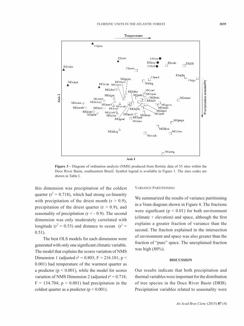
The most highly correlated variables (r2 > 0.6) with the NMS dimensions are shown in Table III. The first dimension was effective in the segregation of sites

along a thermal gradient, so that warmer sites were positioned to the right and colder sites to the left in the ordination diagram (Fig. 3). The variable most highly correlated with this dimension was mean temperature of the warmest quarter (r2 = 0.803), which was strongly co-linear with elevation (r < - 0.9), the aridity index (r < - 0.9), and the following thermal variables (r > 0.9): mean temperature of the coldest quarter, mean temperature of the driest quarter, mean temperature of the wettest quarter, minimum temperature of the coldest month, and maximum temperature of the warmest month. Note that co-linearity is not critical here because we are dealing with an initial exploratory analysis instead of any inferential test.

The second NMS dimension summarizes the segregation of sites along a gradient of precipitation seasonality, with sites showing lower seasonality (1-3 months) occupying the upper portion of the diagram, and sites with higher seasonality (4-5 months) occupying the lower portion of the diagram (Fig. 2). The variable most highly correlated with

TABLE III Environmental variables more correlated (r2 > 0.6) to ordination dimensions created from

floristic data of 55 sites within the Doce River Basin, southeastern Brazil. Bold numbers are correlation values of pre-selected variables for construction of linear models.

Dimension 1 Dimension 2Environmental variables r r2 r r2

Elevation -0.891 0.795 -0.041 0.002Annual mean temperature 0.895 0.801 0.028 0.001Max. temperature of the warmest month 0.873 0.763 -0.094 0.009Min. temperature of the coldest month 0.859 0.738 0.268 0.072Mean temperature of the wettest quarter 0.881 0.777 -0.006 0Mean temperature of the driest quarter 0.883 0.780 0.130 0.017Mean temperature of the warmest quarter 0.896 0.803 -0.004 0Mean temperature of the coldest quarter 0.885 0.783 0.127 0.016Precipitation of the driest month 0.174 0.030 0.831 0.691Precipitation seasonality -0.257 0.066 -0.802 0.644Precipitation of the driest quarter 0.151 0.023 0.832 0.693Precipitation of the coldest quarter 0.054 0.003 0.847 0.718Severity of the water deficit 0.213 0.045 -0.781 0.610Aridity index -0.792 0.627 0.119 0.014



this dimension was precipitation of the coldest quarter (r2 = 0.718), which had strong co-linearity with precipitation of the driest month (r > 0.9), precipitation of the driest quarter (r > 0.9), and seasonality of precipitation (r < - 0.9). The second dimension was only moderately correlated with longitude (r2 = 0.53) and distance to ocean (r2 = 0.51).

The best OLS models for each dimension were generated with only one signifi cant climatic variable. The model that explains the scores variation of NMS Dimension 1 (adjusted r² = 0.803; F = 216.181; p < 0.001) had temperature of the warmest quarter as a predictor (p < 0.001), while the model for scores variation of NMS Dimension 2 (adjusted r² = 0.718; F = 134.704; p < 0.001) had precipitation in the coldest quarter as a predictor (p < 0.001).

varianCe Partitioning

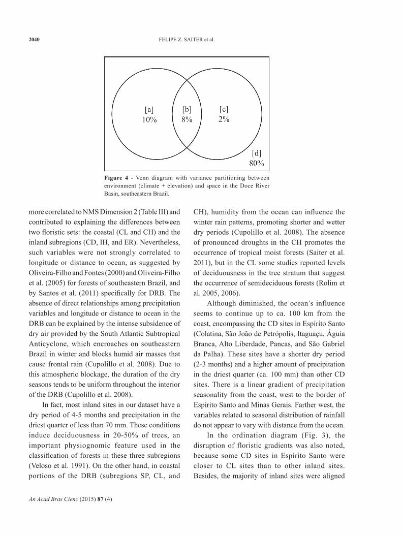
We summarized the results of variance partitioning in a Venn diagram shown in Figure 4. The fractions were signifi cant (p < 0.01) for both environment (climate + elevation) and space, although the fi rst explains a greater fraction of variance than the second. The fraction explained in the intersection of environment and space was also greater than the fraction of “pure” space. The unexplained fraction was high (80%).

DISCUSSION

Our results indicate that both precipitation and thermal variables were important for the distribution of tree species in the Doce River Basin (DRB). Precipitation variables related to seasonality were

Figure 3 - Diagram of ordination analysis (NMS) produced from fl oristic data of 55 sites within the Doce River Basin, southeastern Brazil. Symbol legend is available in Figure 1. The sites codes are shown in Table I.



more correlated to NMS Dimension 2 (Table III) and contributed to explaining the differences between two fl oristic sets: the coastal (CL and CH) and the inland subregions (CD, IH, and ER). Nevertheless, such variables were not strongly correlated to longitude or distance to ocean, as suggested by Oliveira-Filho and Fontes (2000) and Oliveira-Filho et al. (2005) for forests of southeastern Brazil, and by Santos et al. (2011) specifi cally for DRB. The absence of direct relationships among precipitation variables and longitude or distance to ocean in the DRB can be explained by the intense subsidence of dry air provided by the South Atlantic Subtropical Anticyclone, which encroaches on southeastern Brazil in winter and blocks humid air masses that cause frontal rain (Cupolillo et al. 2008). Due to this atmospheric blockage, the duration of the dry seasons tends to be uniform throughout the interior of the DRB (Cupolillo et al. 2008).

In fact, most inland sites in our dataset have a dry period of 4-5 months and precipitation in the driest quarter of less than 70 mm. These conditions induce deciduousness in 20-50% of trees, an important physiognomic feature used in the classifi cation of forests in these three subregions (Veloso et al. 1991). On the other hand, in coastal portions of the DRB (subregions SP, CL, and

CH), humidity from the ocean can infl uence the winter rain patterns, promoting shorter and wetter dry periods (Cupolillo et al. 2008). The absence of pronounced droughts in the CH promotes the occurrence of tropical moist forests (Saiter et al. 2011), but in the CL some studies reported levels of deciduousness in the tree stratum that suggest the occurrence of semideciduous forests (Rolim et al. 2005, 2006).

Although diminished, the ocean’s influence seems to continue up to ca. 100 km from the coast, encompassing the CD sites in Espírito Santo (Colatina, São João de Petrópolis, Itaguaçu, Águia Branca, Alto Liberdade, Pancas, and São Gabriel da Palha). These sites have a shorter dry period (2-3 months) and a higher amount of precipitation in the driest quarter (ca. 100 mm) than other CD sites. There is a linear gradient of precipitation seasonality from the coast, west to the border of Espírito Santo and Minas Gerais. Farther west, the variables related to seasonal distribution of rainfall do not appear to vary with distance from the ocean.

In the ordination diagram (Fig. 3), the disruption of floristic gradients was also noted, because some CD sites in Espírito Santo were closer to CL sites than to other inland sites. Besides, the majority of inland sites were aligned

Figure 4 - Venn diagram with variance partitioning between environment (climate + elevation) and space in the Doce River Basin, southeastern Brazil.



along NMS Dimension 1, indicating that floristic variations among subregions were more correlated to temperature associated with elevation than with seasonal distribution of precipitation.

We noticed that the strong correlation of NMS Dimension 1 with elevation and temperature variables suggests a thermal control in the species distribution following elevational gradients in both coastal and inland portions of the DRB. The ecological effect of elevation is related to its influence on geophysical factors that directly affect plant growth, such as air pressure, wind, humidity, insolation, and temperature (Grubb et al. 1977, Körner 2007). Adaptations of species to different levels of these factors drive the floristic composition along altitudinal gradients (Grubb 1977, Pausas and Austin 2001, Scarano 2002, Kessler et al. 2011).

Studies have reported the high elevation characteristics of the tree flora in the Atlantic Forest of southeastern Brazil. High richness of Asteraceae, Lauraceae, Myrtaceae, Melastomataceae, Rubia-ceae and Solanaceae (França and Stehmann 2004, Saiter et al. 2011), and occurrence of genera such as Clethra, Clusia, Drimys, Hedyosmum, Ilex,

Meliosma, Meriania, Miconia, Myrceugenia, Podocarpus, Prunus, Roupala, and Weinmannia (Giulietti and Pirani 1988, Oliveira-Filho and Fontes 2000) are considered diagnostic of highland forests in such region. In fact, we noticed several species of these families and genera among the indicator species of highland floristic units (i.e., CH, IH plus ER, and Canga, see Table IV).

At lower elevations (in general < 600 m), Euphorbiaceae, Leguminosae, and Sapotaceae are the richest and most abundant families, although some genera of Lauraceae (mainly Ocotea) and Myrtaceae (Eugenia, Marlierea, and Myrcia) are still represented by many species (Guedes-Bruni et al. 2006, França and Stehmann 2013, Lombardi and Gonçalves 2000, Rolim et al. 2006). In turn, indicator species of low-elevation units (SP, CL, and CD) mostly belong to these families and genera (see Table IV).

These characteristics support the significant differences found in NMS Dimension 1 between the CL and the CH, and between the CD and the IH plus ER. Considering this last case, we were unable to find significant differences between the IH and ER, despite some distinctive environmental

TABLE Iv Indicator species of six floristic units within the Doce River Basin, southeastern Brazil.

Sandy Coastal Plain: Abarema filamentosa, Aspidosperma pyricollum, Calyptranthes brasiliensis, Clusia hilariana, Clusia spiritu-sanctensis, Eugenia astringens, Leptolobium bijugum, Maytenus obtusifolia, Myrsine parvifolia, Ocotea cernua, Protium icicariba.Coastal Lowland: Amphirrhox longifolia, Annona acutiflora, Aspidosperma camporum, Aspidosperma discolor, Byrsonima cacaophila, Campomanesia espiritosantensis, Couepia carautae, Couepia schottii, Diplotropis incexis, Eugenia copacabanensis, Exellodendron gracile, Exostyles venusta, Glycydendron espiritosantense, Guazuma crinita, Henriettea succosa, Hirtella bahiensis, Inga tripa, Licania salzmannii, Manilkara salzmannii, Marlierea strigipes, Marlierea suaveolens, Maytenus samydaeformis, Miconia mirabilis, Micropholis guyanensis, Myrcia isaiana, Neomitranthes obtusa, Ocotea aniboides, Ocotea confertiflora, Ormosia nitida, Parkia pendula, Pilocarpus grandiflorus, Plinia stictophylla, Pouteria bapeba, Simira grazielae, Tabernaemontana salzmannii, Tovomita brevistaminea, Xylopia ochrantha.Coastal highland: Baccharis dentata, Byrsonima ligustrifolia, Clusia lanceolata, Clusia organensis, Drimys brasiliensis, Matayba sylvatica, Meliosma chartacea, Meliosma sellowii, Miconia pusilliflora, Psychotria suterella, Solanum megalochiton, Solanum pseudo-quina, Solanum rufescens, Tibouchina arborea, Vantanea compacta.Central Depression: Carpotroche brasiliensis, Casearia guianensis, Gallesia integrifolia, Joannesia princeps, Machaerium incorruptibile, Machaerium pedicellatum, Miconia calvescens, Pseudopiptadenia contorta, Sparattosperma leucanthum.Interior highland plus Espinhaço Range: Blepharocalyx salicifolius, Callisthene major, Casearia obliqua, Eremanthus incanus, Ixora brevifolia, Lamanonia ternata, Matayba mollis, Tapirira obtusa, Vochysia tucanorum.Canga of southernmost Espinhaço Range: Athenaea pereirae, Baccharis lychnophora, Cinnamomum erythropus, Eremanthus crotonoides, Hololepis pedunculata, Ilex pseudobuxus, Myrceugenia myrcioides, Pseudobrickellia angustissima, Schefflera varisiana, Trembleya laniflora, Weinmannia humilis.



conditions in our dataset, such as the fact that ER sites are located at higher elevations and in colder and rainier places than the IH sites. Physiognomic differences are remarkable between the IH, where forests predominate, and the ER, where shallow, sandy and dry soils, induce the dominance of savannas (‘campos rupestres’; Giulietti and Pirani 1988, Kamino et al. 2008). In the ER, forests occur in islands (‘capões’) or are connected to valley forests, where deeper and moister soils allow the development of trees 7-15 meters in height (Giulietti and Pirani 1988, Kamino et al. 2008).

The absence of significant differences, however, indicates that forests in the ER share many tree species with the IH forests, i.e., those able to tolerate low temperatures and shallow, dry soils; these are probably the indicator species of the unit IH plus ER. The resemblance among the IH and ER forest sites agrees with Carmo and Jacobi (2013), Giulietti and Pirani (1988), and Kamino et al. (2008) regarding strong influences of Atlantic Forest Domain on the tree flora in forest patches and gallery forests of Espinhaço Range.

The SP was treated differently because the sites, due to their lower floristic richness when compared to other subregions, were considered outliers. The flora of the SP was derived from the migration of taxa from the mesic coastal forests (Rizzini 1997), but its floristic poverty may be explained by the insufficient time for speciation (Scarano 2002), since its origin is the Upper Quaternary after the last transgression occurred ca. 5,100 yr BP (Martin et al. 1993). Despite this, the three sites of the SP formed a distinct group in cluster analysis, supporting the floristic identity of this subregion.

Another outlier case involved the Canga site of the southernmost ER that hosts forest patches on ironstone outcrops. This site comprises a group separated from other ER sites in the dendrogram (Fig. 2). Here, the richness of the tree stratum is lower than in other ER forests (Kamino et al.

2008), and can be explained by evolutionary selection for taxa that can tolerate low temperatures and substrates with a high percentage of toxic metals (metalophyte functional group; Carmo and Jacobi 2013). In fact, some indicator species of the Canga belong to metalophyte genera recognized by Carmo and Jacobi (2013), such as Eremanthus, Ilex, Trembleya, and Weinmannia. Notwithstanding this poverty in tree species, high levels of both richness and endemism have been recorded in the herbaceous and shrubby strata of Canga (Jacobi and Carmo 2008, Carmo and Jacobi 2013).

The influence of spatial proximity in the patterns reported here cannot be disregarded. Although environmental factors have been very important in the explanation of floristic variation, the fraction explained purely by space was significant as well. We also assumed that the fraction explained by spatial processes was not overestimated because an extensive set of environmental predictors were also used. Therefore, the distribution of tree species along the DRB could be determined in part by their dispersal limitation. In addition, an important portion of the floristic variation can be attributed to environmental resemblances among sites that are geographically close (the spatially structured environment).

The high unexplained fraction (80%) of the floristic variation can be attributed to undetermined residuals related to variables that were not included in the analyses. In general, biotic interactions (including anthropogenic effects) and historical events are not included in biogeographical analyses due to the difficulty of quantifying them (Zimmermann et al. 2010); this exclusion is relatively common in vegetation studies (ter Braak 1987).

We can conclude, therefore, that: [1] Thermal variables (particularly temperature of the warmest quarter), associated with precipitation variables (particularly precipitation of the coldest quarter), were the most important factors for determining



tree species distribution in the DRB; [2] Site spatial proximity significantly influenced the explanation of patterns due to the limited dispersal of species and spatially structured climatic variables; [3] Considering floristic and environmental features, the subregions SP, CL, CH and CD can be treated as distinct floristic units. The subregions IH and ER, however, should be recognized as a single floristic unit encompassing most of interior highlands. Furthermore, the ‘cangas’ of the southernmost ER should be considered as a distinct unit due to their unique ecological features as suggested by Jacobi and Carmo (2008).

Although general phytogeographic patterns can provide theoretical support for conservation planning in the Atlantic Forest at a coarse level, the stakeholders (mainly the government and conservation organizations) should always be aware of the ecological criteria determining discrete floristic units within a given region. Even if the floristic knowledge is insufficient, consideration of geomorphology and climate at finer scales in subregions defined for other purposes (e.g., geopolitics or water management) can lead to wiser biodiversity conservation planning. Parks and reserves should be created in each of these subregions, in order to protect most of the plant species, especially the endemic and indicator ones. In forest restoration, species selection should respect the tree composition in nearby forests that are floristically similar.

ACKNOWLEDGMENTS

Felipe Z. Saiter thanks the Coordenação de Aperfeiçoamento de Pessoal de Nível Superior (CAPES) for the Sandwich Fellowship. Ary T. de Oliveira-Filho, João R. Stehmann and Pedro V. Eisenlohr thank the Conselho Nacional de Desenvolvimento Científico e Tecnológico (CNPq) for support. William W. Thomas thanks the National Science Foundation (DEB 0946618) for support.

RESUMO

Nós submetemos dados geoclimáticos e de ocorrência de espécies arbóreas de 59 sítios em uma bacia hidrográfica na Mata Atlântica do sudeste do Brasil a análises de ordenação, ANOVA e agrupamento com os objetivos de investigar as causas dos padrões fitogeográficos e determinar se as seis sub-regiões reconhecidas constituem unidades florísticas distintas. Nós descobrimos que clima e espaço foram significativamente (p ≤ 0,05) importantes na explicação dos padrões fitogeográficos. As variações florísticas seguem gradientes térmicos ligados à altitude tanto em sub-regiões costeiras como interioranas. Um gradiente de sazonalidade da precipitação esteve relacionado com a variação florística até 100 km para o interior a partir do oceano. A temperatura no trimestre mais quente e a precipitação durante o trimestre mais frio foram os principais preditores. As sub-regiões Planície Arenosa Costeira, Terra Baixa Costeira, Montanha Costeira, e Depressão Central foram reconhecidas como unidades florísticas distintas. Diferenças significativas não foram encontradas entre Montanha do Interior e Cadeia do Espinhaço, indicando que essas sub-regiões devem compor uma única unidade florística abrangendo todas as áreas elevadas do interior. Por causa de suas peculiaridades ecológicas, os campos ferruginosos no interior da Cadeia do Espinhaço podem constituir uma unidade especial. As unidades florísticas aqui propostas fornecerão informações importantes para o sábio planejamento da conservação no hotspot Mata Atlântica.

Palavras-chave: Padrões fitogeográficos, gradientes ambientais, autocorrelação espacial, bacia do Rio Doce.

REFERENCES

BertonCeLLo r, yaMaMoto K, MeireLes Ld and shePherd gJ. 2011. A phytogeographic analysis of cloud forests and other forest subtypes amidst the Atlantic forests in south and southeast Brazil. Biodivers Conserv 20: 3413-3433.

BLanChet Fg, Legendre P and BorCard d. 2008. Modelling directional spatial processes in ecological data. Ecol Model 215: 325-336.

BorCard d, giLLet F and Legendre P. 2011. Numerical Ecology with R. New York: Springer, 306 p.

BreCKLe SW. 2002. Walter’s Vegetation of the EartINh: the Ecological Systems of the Geo-Biosphere. 4th ed., Berlin: Springer-Verlag, 527 p.



BurnhaM KP and anderson dr. 2002. Model selection and multimodel inference. A practical information-theoretical approach. New York: Springer-Verlag, 487 p.

CarMo FF and JaCoBi CM. 2013. A vegetação de canga no Quadrilátero Ferrífero, Minas Gerais: caracterização e contexto fitogeográfico. Rodriguésia 64(3): 527-541.

Chain-guadarraMa a, Finegan B, viLChez s and Casanoves F. 2012. Determinants of rain-forest foristic variation on an altitudinal gradient in southern Costa Rica. J Trop Ecol 28(5): 463-481.

CuPoLiLLo F, aBreu ML and vianeLLo rL. 2008. Climatologia da bacia do rio Doce e sua relação com a topografia local. Geografias 4(1): 45-60.

dray s, Legendre P and Peres-neto Pr. 2006. Spatial modelling: a comprehensive framework for principal coordinate analysis of neighbour matrices (PCNM). Ecol Model 196: 483-493.

eisenLohr Pv. 2013. Challenges in data analysis: pitfalls and suggestions for a statistical routine in vegetation ecology. Braz J Bot 36(1): 83-87.

eisenLohr Pv. 2014. Persisting challenges in multiple models: a note on commonly unnoticed issues regarding collinearity and spatial structure of ecological data. Braz J Bot 37(3): 365-371.

engeLBreCht BMJ, CoMita Ls, Condit r, Kursar ta, tyree Mt, turner BL and huBBeLL sP. 2007. Drought sensitivity shapes species distribution patterns in tropical forests. Nature 447: 80-83.

Fortin MJ and daLe MRT. 2005. Spatial analysis. A guide for ecologists. Cambridge: Cambridge University Press, 369 p.

França gs and stehMann Jr. 2004. Composição florística e estrutura do componente arbóreo de uma floresta altimontana no município de Camanducaia, Minas Gerais, Brasil. Rev Bras Bot 27(1): 19-30.

França gs and stehMann Jr. 2013. Florística e estrutura do componente arbóreo de remanescentes de Mata Atlântica do médio rio Doce, Minas Gerais, Brasil. Rodriguésia 64(3): 607-624.

gasPer aL, eisenLohr Pv and saLino a. 2013. Climate-related variables and geographic distance affect fern species composition across a vegetation gradient in a shrinking hotspot. Plant Ecol Divers 8(1): 25-35.

giuLietti aM and Pirani Jr. 1988. Patterns of geographic distribution of some plant species from the Espinhaço Range, Minas Gerais and Bahia, Brasil. In: Heyer WR and Vanzolini PE (Eds), Proceedings of a workshop on neotropical distribution patterns. Rio de Janeiro: Academia Brasileira de Ciências, p. 39-69.

guedes-Bruni rr, siLva neto sJ, MoriM MP and Mantovani W. 2006. Composição florística e estrutura de trecho de Floresta Ombrófila Densa Atlântica Aluvial

na Reserva Biológica de Poço das Antas, Silva Jardim, Rio de Janeiro, Brasil. Rodriguésia 57(3): 413-428.

gruBB PJ. 1977. Control of forest growth and distribution on wet tropical mountains, with special reference to mineral nutrition. Ann Rev Ecol Evol Syst 8: 83-107.

hiJMans rJ, CaMeron se, Parra JL, Jones Pg and Jarvis a. 2005. Very high resolution interpolated climate surfaces for global land areas. Int J Clim 25: 1965-1978.

hoMeier J, BreCKLe s, günter s, roLLenBeCK rt and LeusChner C. 2010. Tree diversity, forest structure and productivity along altitudinal and topographical gradients in a species-rich ecuadorian montane rain forest. Biotropica 42(2): 140-148.

instituto Jones dos santos neves. 2012. Mapeamento geomorfológico do Estado do Espírito Santo. Nota Técnica 28. Vitória: Instituto Jones dos Santos Neves, 19 p.

instituto Mineiro de gestão das águas. 2010. Plano integrado de recursos hídricos da bacia hidrográfica do rio Doce. v 1. Belo Horizonte: IGAM – Ecoplan-Lume, 478 p.

JaCoBi CM and CarMo FF. 2008. Diversidade dos campos rupestres ferruginosos no Quadrilátero Ferrífero, MG. Megadiversidade 4(1-2): 25-33.

Jones P and harris i. 2008. CRU Time Series (TS) high resolution gridded datasets. Londres: University of East Anglia Climate Research Unit, NCAS British Atmospheric Data Centre. http://www.cru.uea.ac.uk/cru/data/

KaMino LHY, oLiveira-FiLho at and stehMann Jr. 2008. Relações florísticas entre as fitofisionomias florestais da Cadeia do Espinhaço, Brasil. Megadiversidade 4(1-2): 39-49.

KeLeJian hh and PruCha ir. 2010. Specification and Estimation of Spatial Autoregressive Models with Autoregressive and Heteroskedastic Disturbances. J Econometrics 157(1): 53-67.

KessLer M, grytnes Ja, haLLoy SRP, KLuge J, KröMer t, León B, MaCía MJ and young Kr. 2011. Gradients of plant diversity: local patterns and processes. In: Herzog SK et al. (Eds), Climate change and biodiversity in the tropical Andes. São José dos Campos: Inter-American Institute for Global Change Research – Scientific Committee on Problems of the Environment, p. 204-219.

Körner C. 2007. The use of ‘altitude’ in ecological research. TRENDS Ecol Evol 22(11): 569-574.

Landeiro vL and Magnusson We. 2011. The geometry of spatial analyses: implications for conservation biologists. Nat Conservação 9(1): 7-20.

Legendre P and Fortin MJ. 1989. Spatial pattern and ecological analysis. Vegetatio 80: 107-138.

Legendre P and gaLLagher ed. 2001. Ecologically meaningful transformations for ordination of species data. Oecologia 129: 271-280.



Legendre P and Legendre L. 2012. Numerical ecology, 3rd ed., Developments in Environmental Modelling, v. 24. Amsterdam: Elsevier Science BV, 1006 p.

LePš J and šMiLauer JP. 2003. Multivariate analysis of ecological data using CANOCO. Cambridge: Cambridge University Press, 269 p.

LoMBardi Ja and gonçaLves M. 2000. Composição florística de dois remanescentes de Mata Atlântica do sudeste de Minas Gerais, Brasil. Rev Bras Bot 23(3): 255-282.

Martin L, suguio K and FLexor JM. 1993. As flutuações de nível do mar durante o Quaternário Superior e a evolução geológica de “deltas” brasileiros. Bol IG-USP 15: 1-186.

MCCune B and graCe JB. 2002. Analysis of ecological communities. Gleneden Beach: MjM Software Design, 304 p.

MCCune B and MeFFord MJ. 2011. PC-ORD, Multivariate analysis of ecological data, Version 6. Gleneden Beach: MjM Software Design.

MCshea WJ. 2014. What are the roles of species distribution models in conservation planning? Environ Conserv 41(2): 93-96.

nasCiMento FM, saraiva ALBC, CoeLho ALN and Correa WSC. 2012. Espacialização e análise das temperaturas e precipitações médias anuais do Espírito Santo com o uso de geotecnologias. Rev Geonorte 2(5): 1328-1338.

oKsanen J, BLanChet Fg, Kindt r, Legendre P, MinChin Pr, o’hara rB, siMPson gL, soLyMos P, stevens MHH and Wagner h. 2013. Vegan: Community Ecology Package. http://vegan.r-forge.r-project.org/

oLiveira-FiLho at. 2014. NeoTropTree, flora arbórea da região neotropical: um banco de dados envolvendo biogeografia, diversidade e conservação. Universidade Federal de Minas Gerais. http://www.icb.ufmg.br/treeatlan/

oLiveira-FiLho at and Fontes MAL. 2000. Patterns of Floristic Differentiation among Atlantic Forests in Southeastern Brazil and the Influence of Climate. Biotropica 32(4b): 793-810.

oLiveira-FiLho at, taMeirão-neto e, CarvaLho WAC, WerneCK M, Brina ae, vidaL Cv, rezende sC and Pereira JAA. 2005. Análise florística do compartimento arbóreo de áreas de Floresta Atlântica sensu lato na região das bacias do leste (Bahia, Minas Gerais, Espírito Santo e Rio de Janeiro). Rodriguésia 56(87): 185-235.

Pausas Jg and austin MP. 2001. Patterns of plant species richness in relation to different environments: An appraisal. J Veg Sci 12: 153-166.

Peres-neto Pr and Legendre P. 2010. Estimating and controlling for spatial autocorrelation in the study of ecological communities. Global Ecol Biogeogr 19: 174-184.

Quinn gP and Keough MJ. 2002. Experimental design and data analysis for biologists. Melbourne: Cambridge University Press, 556 p.

rangeL tF, diniz-FiLho JAF and Bini LM. 2010. SAM: A comprehensive application for Spatial Analysis in Macroecology. Ecography 33: 1-5.

r Core teaM. 2011. R: A language and environment for statisticalcomputing. Vienna: R Foundation for Statistical Computing. http://www.r-project.org/

rizzini Ct. 1997. Tratado de Fitogeografia do Brasil. 2ª ed., Rio de Janeiro: Âmbito Cultural Edições Ltda, 747 p.

roLiM sg, Jesus rM, nasCiMento HEM, Couto HTZ and ChaMBers JQ. 2005. Biomass change in an Atlantic tropical moist forest: the ENSO effect in permanent sample plots over a 22-year period. Oecologia 142: 238-246.

roLiM sg, ivanausKas nM, rodrigues rr, nasCiMento Mt, goMes JML, FoLLi da and Couto HTZ. 2006. Composição Florística do estrato arbóreo da Floresta Estacional Semidecidual na Planície Aluvial do rio Doce, Linhares, ES, Brasil. Acta Bot Bras 20(3): 549-561.

saiter Fz, guiLherMe FAG, thoMaz Ld and Wendt t. 2011. Tree changes in a mature rainforest on the Brazilian coast. Biodivers Conserv 20: 1921-1949.

santos MF, seraFiM h and sano Pt. 2011. An analysis of species distribution patterns in the Atlantic Forests of Southeastern Brazil. Edin J Bot 68(3): 373-400.

sCarano Fr. 2002. Structure, function and floristic relationships of plant communities in stressful habitats marginal to the brazilian Atlantic rainforest. Ann Bot 90: 517-524.

sCudeLLer vv, Martins Fr and shePherd gJ. 2001. Distribution and abundance of arboreal species in the atlantic ombrophilous dense forest in Southeastern Brazil. Plant Ecol 152: 185-199.

sMith ra. 1971. The effect of unequal group size on Tukey’s HSD procedure. Psychometrika 36(1): 31-34.

soBraL M and stehMann Jr. 2009. An analysis of new angiosperm species discoveries in Brazil

(1990-2006). Taxon 58(1): 227-232.ter BraaK CJF. 1987. Ordination. In: Jongman RHG et al.

(Eds), Data analysis in community and landscape ecology. Wageningen: Pudoc, p. 91-173.

tiChý L and Chytrý M. 2006. Statistical determination of diagnostic species for site groups of unequal size. J Veg Sci 17: 809-818.

torres rB, Martins Fr and gouvêa LSK. 1997. Climate, soil and tree flora relationships in forests in the state of São Paulo, southeastern Brazil. Rev Bras Bot 20(1): 41-49.

veLoso hP, rangeL FiLho ALR and LiMa JCA. 1991. Classificação da vegetação brasileira, adaptada a um sistema universal. Rio de Janeiro: IBGE, Departamento de Recursos Naturais e Estudos Ambientais, 124 p.



WaLter h. 1985. Vegetation of the earth and ecological systems of the geo-biosphere, 3rd ed., Berlin: Springer-Verlag, 318 p.

White da and hood Cs. 2004. Vegetation patterns and environmental gradients in tropical dry forests of the northern Yucatan Peninsula. J Veg Sci 15: 151-160.

WuLF h, BooKhagen B and sCherLer d. 2010. Seasonal precipitation gradients and their impact on fluvial sediment flux in the Northwest Himalaya. Geomorphology 118: 13-21.

zar Jh. 2010. Biostatistical analysis. 5th ed., Upper Saddle River: Pearson Prentice-Hall, 944 p.

ziMMerMann ne, edWards Jr tC, grahaM Ch, PearMan PB and svenning JC. 2010. New trends in species distribution modelling. Ecography 33: 985-989.

zoMer rJ, Bossio da, traBuCCo a, yuanJie L, guPta dC and singh vP. 2007. Trees and water: small holder agroforestry on irrigated lands in northern India. IWMI Research Report 122. Colombo: International Water Management Institute, 47 p.

Documents

Floristic units and their predictors unveiled in part of … 4930, Jardim Flamboyant, 78580-000 Alta Floresta, MT, Brasil 3Instituto Federal de Educação, Ciência e Tecnologia do