Embed Size (px)
Citation preview

Final Master Thesis
Flood Impact Analysis using GIS
A case study for Lake Roxen and Lake Glan-Sweden
by
Vimalkumar A. Vaghani
2005-06-08
ISRN: LIU-IDA-D20--05/016--SE


Linköpings universitet Institutionen för datavetenskap
Final Master Thesis
Flood Impact Analysis using GIS
A case study for Lake Roxen and Lake Glan-Sweden
by
Vimalkumar A. Vaghani
2005-06-08
ISRN: LIU-IDA-D20--05/016--SE
Supervisor : Dr. Åke Sivertun, IDA, Linköpings universitet Examiner : Dr. Åke Sivertun, IDA, Linköpings universitet


Dedicated to my PARENTS
Shri Ajitkumar Amrutlal Vaghani
Smt. Jyotiben Ajitkumar Vaghani
&
GOD

For, Rolf Karlsson and Louise Nordström

Abstract
Floods are common natural disaster occurring in most parts of the world. This results in
damage to human life and deterioration of environment. There have been immense uses of
technology to mitigate measures of flood disaster i.e. structurally and non-structurally.
Undoubtedly, structural measures are very expensive and time consuming which involves
physical work like construction of dams, reservoirs, bridges, channel improvement, river
diversion and other embankments to keep floods away from people. Whereas non-structural
measures is concerned with planning like flood forecasting and warning, flood plain zoning,
relief and rehabilitation for reducing the risk of flood damage to keep people away from
floods. Thus, non-structural measures involve analysis, planning providing spatial information
on maps with high accuracy in less time. Non-structural measures can help decision maker to
plan an effective emergency response towards flood disaster. A one of the good way to plan
non-structural measures is to analyze impact of flood in the flood prone areas. The thesis tries
to analyze impact of flood on environment along the demarcated flood prone areas of Lake
Roxen and Lake Glan in Östergötland County, Sweden. The thesis also proposes how to use
current flood information during flood emergency utilizing geographical information system.
This provides spatial information for area in the flood zone for assessment regarding flood
vulnerability.
Using map overlay analysis in GIS software (ArcGIS); flood prone areas and topographic
data along Lake Roxen and Lake Glan were digitized from PDF maps. Thus, the thesis work
is an effort to analyze impact of flood when areas along Lake Roxen and Lake Glan are
flooded. ESRI® GIS software Arc Map 9 and Arc View 3.3 is used for data preparation,
integrating, analyzing, and spatial data with attribute table information. Finally, to show GIS
can be an effective tool for development of flood emergency system as a part of disaster
preparedness by the decision makers.
Keywords: Analysis, Data set, Decision-maker, Digitized, Disaster, Environment, Flood,
Geographical information system (GIS), Georeferenced, Hazard zone, Impact , Lake Roxen
and Lake Glan, Remote Sensing, Risk, River, Spatial overlay analysis, Sweden, Emergency,
Vulnerable.
i

ii
Acknowledgements I would like to thank my supervisor and examiner Dr.Åke Sivertun for his kind guidance, providing different solution and motivation towards my master thesis. He has been a person who have suggested and introduced me to how to work with my topic of interest using GIS and how to enhance my skills. He have provided his valuable time in discussing, going through my drafts, providing comments and advices to improve my work from time to time. Also apart from my supervisor, I would like to thank some professional person from different organization and institution for their suggestion, comments, information, materials and other help. They are Hans Eriksson (Norrköping Fire and Rescue Service – Brandförsvar), Bodil Karlsson and Barbro Näslund-Landenmark (Swedish Rescue Services Agency), Jonas Sjölin (Chef director of GIS Unit in Norrköpings Commune), Sören Almgren (Swedish National Land Survey, Lantmäteriet), Holst Bo, Lindström Göran, Sanner Håkan and Yacoub Tahsin (Swedish Metrological and Hydrological Institute, SMHI). Jalal Maleki, Helene Wigert, Michael Le Duc, Jiri Trnka & Susanna Nilsson from (IDA-LiU), Lotta Andersson & Julie Wilk from (Tema Vatten, Linköping University) Rolf Karlsson and Louise Nordström my Swedish host family, who have provided me unforgettable memories with them and their family members. I will always be thankful to them in my life for all their teaching and support during my stay in Sweden and Finland. Jörgen Hammarstedt (Kreatel), Christina Hammarstedt, Gunilla Desai, Benny Karlsson (Vattenfall, Stockholm), Ulla Karlsson (Åre commune, Åre) Kjell Wester (Swed Power, Stockholm) and Gunnar Westberg (Swedish Geotechnical Institute - SGI, Linköping) as my well wisher My big thanks go to Kamila Belka and Mr. Shashikant Kumar (Green Eminent Consultant) for helping me in understanding the subject well. Thanks go to my friend and opponent Jayabharath Kumar Suri who always supported me to finish my studies and helped me in many ways from time to time and my other opponent Mohamed Ahmed Osman. Also my thanks to Muhammad Hassan who helped me formulate my ideas of carrying my thesis and to all classmates and former colleagues during my studies at Master’s Program of Geoinformatics 2004-05, namely Aleksander Gumos, Amit Sharma, Anilkumar Koyalkar, Anwar Moghal, Azza Salah Eldin Ali, Bharath Gupta, Kamal Pathak, Mohamed Soghayroon, Rahel Hamad, Raja Ramesh Bhogavally and Sabina Alexandriu. Thanks to my friends back home Amrish, Ajay, Mitesh, Mohsin, Rakesh, Ranjit and Shweta. Many thanks to Swedish Rescue Agency – Räddningsverket (SRV), Lantmäteriet, Swedish Geological Survey (SGU), and Swedish Metrological and Hydrological Institute (SMHI) for various support and to the Department of Computer and Information Science (IDA), Linköping University for allowing using GIS lab, staff and library facilities to carry out my master thesis. I would like to use the opportunity to thank the State Bank of India (SBI), Baroda-Gujarat, India for financial support to me so that I was able to concentrate on my studies and research. Finally, I wish to express my deep gratitude to my parents and sisters as well as colleagues back home in India for their great support. I would like to specially thank Dr. Rolee Kanchan (Lecturer) and Dr. Jayasree De (Head and Professor Dept of Geography, The M.S.University of Baroda), Rupesh Rajpurohit (Centre for Environmental Planning & Technology, CEPT), Shri Ajitkumar, Smt. Jyotiben, Smt. Mittalben, Kum. Kuntalben, Smt. Sejalben, Kum. Riya, Mr. Bipin kumar, Mr. Mitesh kumar, Shri Jagdish Khara, Shri Mahendra Khara, Shri Atul Shah.
iii

iv

Table of contents
Abstract ...................................................................................................................................... i
Acknowledgements..................................................................................................................iii
Table of contents....................................................................................................................... v
List of figures ..........................................................................................................................vii
List of tables............................................................................................................................. ix
List of acronyms ....................................................................................................................... x
List of appendixes.................................................................................................................... xi
Chapter 1. Introduction........................................................................................................... 1
1.1. Motivation and background ....................................................................................... 1 1.2. Floods in Western Europe and Sweden...................................................................... 2 1.3. The geographical description of study area................................................................ 5 1.4. Location map of study area ........................................................................................ 7 1.5. Objectives................................................................................................................... 8
Chapter 2. Theory .................................................................................................................... 9
2.1. What is Geographic Information System (GIS)? ....................................................... 9 2.1.1. Data models in GIS ......................................................................................... 9 2.1.2. Vector data analysis ...................................................................................... 11
2.2. Impact analysis......................................................................................................... 11 2.2.1. Measurement of impact ................................................................................. 14
2.3. Emergency management .......................................................................................... 18 2.3.1. Emergency response organization in Western Europe.................................. 19 2.3.2. GIS and emergency management in Sweden................................................ 19
2.4. Flood management ................................................................................................... 21 2.4.1. Overview of institutional flood management in Western Europe................. 21
Chapter 3. Methodology ........................................................................................................ 23
3.1. Material .................................................................................................................... 23 3.2. Terminology ............................................................................................................. 23 3.3. Software ................................................................................................................... 23 3.4. Data collections and description .............................................................................. 23 3.5. GIS technique- Flood impact simulation ................................................................. 26
3.5.1. Following are generalized steps followed for flood impact simulation to prepare digitized spatial dataset from pdf map for the study area. ............... 27
3.5.2. Digitizing of layer ......................................................................................... 31 3.5.3. Erasing non flood prone area polygons......................................................... 31 3.5.4. Following are the generalized steps followed for flood impact simulation to
overlay spatial data set with subset (frame) and accurate flood prone area (primary risk areas & 100 years risk area for flood) layer in arc view 3.3 and arc map -arc GIS 9 ........................................................................................ 32
3.5.5. Task performed on each dataset available with the subset area (frame) and primary risk areas and 100 years risk area for flood in arc view 3.3 ............ 33
v

3.5.6. Following are the generalized steps followed for flood impact simulation for updating the attribute table of all spatial database layers in arc map -arc GIS 9 …………………………………………………………………………...34
3.5.7. Pre-processing of data set for subset study area............................................ 39 3.5.8. Following was the final task for flood impact analysis map products in arc
map -arc GIS 9 .............................................................................................. 48 Chapter 4. Results and analysis ............................................................................................ 49
4.1. Flood impact analysis and map products ................................................................. 49 4.1.1. Identification of endangered areas ................................................................ 49 4.1.2. Impact analysis for the affected landuse, road network, soil type and landuse
in points feature............................................................................................. 49 4.1.3. Calculated tables for impact area .................................................................. 58
4.2. Significance of flood impact analysis: ..................................................................... 63 4.2.1. Property data linking ..................................................................................... 63 4.2.2. Emergency planning...................................................................................... 63 4.2.3. Landfill .......................................................................................................... 65 4.2.4. Sharing risk data with public......................................................................... 66
Chapter 5. Discussion and conclusion .................................................................................. 69
5.1. Discussion ................................................................................................................ 69 5.2. Conclusion................................................................................................................ 69 5.3. Further studies .......................................................................................................... 70
References ............................................................................................................................... 71 Appendixes.............................................................................................................................. 79
vi

List of figures
Figure 1: Estimated deviation (1901–2002) in annual average temperature, precipitation and runoff.......................................................................................................................................... 3 Figure 2: A graph showing total number of persons affected (1906-2004) due to flood in Western Europe .......................................................................................................................... 4 Figure 3: The Motala river basin (catchments), Sweden with its sub-basin .............................. 5 Figure 4: Location map of Europe continent showing Sweden country with different läns...... 7 Figure 5: Ostergötland län map with different kommune boundaries; Norrköping, Finspång Linköping kommune with subset area (frame), Lake Roxen and Lake Glan as study area....... 7 Figure 6: Vector and raster model diagram.............................................................................. 10 Figure 7 : A graph showing impact of impact analysis studies................................................ 12 Figure 8: A figure showing major environmental elements (point and non-point source pollution) responsible for water pollution................................................................................ 14 Figure 9: Visualization of flood emergency response.............................................................. 20 Figure 10: Flowchart showing methodology to carry out flood impact analysis..................... 24 Figure 11: Flowchart showing the methodology to prepare geo-referenced digitized spatial data from pdf maps for the study area...................................................................................... 27 Figure 12: A print screen window showing study area in pdf map (karta) 2, 3, 4 and 5 from obtained report.......................................................................................................................... 28 Figure 13: A print screen window showing geo-referencing of tiff images with the existed Lake shapefile in arc map -arc GIS 9....................................................................................... 29 Figure 14: A print screen window showing digitizing of geo-referenced tiff images in arc map -arc GIS 9 ................................................................................................................................. 30 Figure 15: A print screen window showing accurate layers from different digitized layers in arc map -arc GIS 9 ................................................................................................................... 31 Figure 16: Flowchart showing methodology to merge layers and overlay with study area..... 32 Figure 17: A print screen window-showing task performed on each spatial data layer in arc view 3.3 .................................................................................................................................... 34 Figure 18: Adding blank field columns to spatial database layer in study area....................... 35 Figure 19: Adding translated Swedish – English names in blank fields temporally for working window..................................................................................................................................... 35 Figure 20: Adding translated Swedish –English names in blank fields for permanently in attribute table............................................................................................................................ 36 Figure 21: Calculating total area, length or count for each spatial dataset layer in study area 37 Figure 22: Summarizing the attribute table for each spatial dataset layer in study area.......... 38 Figure 23: Exporting summarized dbf tables for each spatial dataset layer of study area into word format .............................................................................................................................. 38 Figure 24: A map showing flood prone areas with study area i.e. total primary risk areas & 100 years risk area for flood along Lake Roxen and Lake Glan.............................................. 39
vii

Figure 25: A map showing clipped soil type with impact subset area..................................... 40 Figure 26: Pie diagram showing total percentage of soil type in impact subset area .............. 40 Figure 27: Bar graph showing total sq. km. area of soil type in impact subset area................ 41 Figure 28: A map showing clipped landuse type map and road network map with impact subset area ................................................................................................................................ 42 Figure 29: Pie diagram showing total percentage of landuse type in impact subset area ........ 43 Figure 30: Bar graph showing total sq. km. area of landuse type in impact subset area ......... 43 Figure 31: Pie diagram showing total percentage of road type in impact subset area ............. 44 Figure 32: Bar graph showing total km. area of road type in impact subset area .................... 45 Figure 33: A map showing clipped landuse in points-buildings, vegetation and hydrography feature with impact subset area ................................................................................................ 46 Figure 34: Pie diagram showing total percentage of landuse in points in impact subset area . 46 Figure 35: Bar graph showing total count landuse in points in impact subset area ................. 47 Figure 36: A map showing affected landuse type along the study area................................... 50 Figure 37: Pie diagram showing total percentage of affected landuse type in impact area ..... 50 Figure 38: A bar graph showing the total affected landuse in primary risk areas and 100 years risk area for flood impact area.................................................................................................. 51 Figure 39: A map showing affected road type along the study area ........................................ 52 Figure 40: Pie diagram showing total percentage of affected road type in impact area .......... 52 Figure 41: A bar graph showing the total affected road type in primary risk areas and 100 years risk area for flood impact area ........................................................................................ 53 Figure 42: A map showing affected soil type along study area ............................................... 54 Figure 43: Pie diagram showing total percentage of affected soil type in impact area............ 54 Figure 44: A bar graph showing the total affected soil type in primary risk areas and 100 years risk area for flood impact area.................................................................................................. 55 Figure 45: A map showing affected landuse in points along the study area............................ 56 Figure 46: Pie diagram showing total percentage of affected landuse in points in impact area.................................................................................................................................................. 56 Figure 47: A bar graph showing total affected landuse in points in primary risk areas and 100 years risk area for flood impact area ........................................................................................ 57 Figure 48: Pie diagram showing total percentage of affected flood prone area in impact area58 Figure 49: OID in landuse theme could be use to link the affected parcel for emergency response planning..................................................................................................................... 63 Figure 50: A print screen window showing evacuation planning for emergencies for shortest path ........................................................................................................................................... 64 Figure 51: Affected landuse and soil type due to landfill selected by overlay analysis using orthophoto image...................................................................................................................... 65
viii

List of tables
Table 1: A table showing major disasters (1976-2005) occurred and its losses in Sweden ...... 4
Table 2: A table showing advantages and disadvantages of impact analysis methods............ 13
Table 3: A table showing checklist for total calculated area in sq m, km and total percentage in subset area (frame) ............................................................................................................... 25
Table 4: A table showing calculated total area of different themes of study area in sq. m. and sq. km. ...................................................................................................................................... 39
Table 5: A table showing calculated total clipped soil types area in sq. m. and sq.km. .......... 41
Table 6: A table showing calculated total clipped landuse types area in sq. m. and sq. km.... 44
Table 7: A table showing calculated total clipped total road network length in m. and km.... 45
Table 8: A table showing calculated total counts of clipped classified landuse in points-buildings, vegetation and hydrography features ...................................................................... 47
Table 9: A table showing total calculated flood prone area and other water bodies in sq. m, sq.km and percentage ............................................................................................................... 58
Table 10: A table showing total affected landuse shapefile in primary risk areas and 100 years risk area for flood calculated in sq.m and sq. km..................................................................... 59
Table 11: A table showing total affected soil type shapefile in primary risk areas and 100 years risk area for flood calculated in sq.m and sq. km ........................................................... 60
Table 12: A table showing total affected road type shapefile in primary risk areas and 100 years risk area for flood calculated in m and km ..................................................................... 61
Table 13: A table showing total number of parcel affected for landuse in points shapefile in primary risk areas and 100 years risk area for flood ................................................................... 62
Table 14: Impact analysis table for different dataset ............................................................... 67
ix

List of acronyms
1. CGIS – Canadian Geographic Information system
2. CRED – Center for Research on the Epidemiology of Disasters
3. DEM – Digital Elevation model
4. DOM – Dissolved Organic Carbon
5. EIA – Environmental Impact Assessment
6. EM – Emergency management
7. EPA – Environmental Protection Agency
8. ESRI – Environmental Systems Research Institute
9. GCS – Geographic co-ordinate system
10. GIS – Geographic information system
11. GSL – Geological Society of London
12. HBV – Hydrologiska Byråns Vattenbalansavdelning
13. ICE – International Chemical Environment
14. IDA – Institutionen för datavetenskap
15. KKOD – Category code
16. NLS – Lantmäteriet (National Land Survey of Sweden)
17. OID –Object identity
18. OID\KKOD – Object ID / Category code of object
19. PAHs – Polycyclic aromatic hydrocarbons
20. PDF – Portable Document Format (Adobe Acrobat)
21. RS – Remote Sensing
22. RT90 – Rikets koordinatsystem 1990
23. SDSS – Spatial Decision Support Systems
24. SGI – Swedish Geotechnical Institute
25. SGU – Swedish Geological Survey
26. SMHI – Swedish Metrological and Hydrological Institute
27. SRV – Swedish Rescue Agency, Räddningsverket
28. UK – United Kingdom
29. UN – United Nation
30. UNEP – United Nations Environment Programme
31. UNDP- United Nations Developmental Programme
32. USLE – Universal Soil Loss Equation
33. VBA – Visual Basic for Applications
x

List of appendixes
Appendix 1. Internet electronic resources:............................................................................... 79
Appendix 2. Questionnaire – verbal interview with personnel................................................ 79
Appendix 3. List of persons consulted for information ........................................................... 80
Appendix 4. Common file format ............................................................................................ 80
Appendix 5. Formula for calculation ....................................................................................... 80
Appendix 6. List of further subcategories of category-classified for road network and landuse in points table ........................................................................................................................... 81
xi


Chapter 1 Introduction
Chapter 1.
1.1.
Introduction
Motivation and background “Disasters do not cause effects; the effects are what we call a disaster” Wolf Dombrowsky (1995) Above quotation conveys a message that the disaster is an effect of an event that brings vulnerability in environment. Thus, it implies that there is a need to study the effects of disasters. Natural disasters are common nowadays in today’s world. They are result of sudden change in state of natural elements due to natural forces. Most of the natural disasters are beyond control of human beings and cannot be predicted accurately when it occurs. Major natural disaster like floods, earthquakes, landslides and droughts when they happen, it result in threat of human life, loss of property; affect infrastructure, agriculture and environment. The impact of disaster is different due to its intensity and coverage area. Floods are the most common occurring natural disasters that affect human and its surrounding environment (Hewitt 1997). It is more vulnerable to Asia and the Pacific regions. It affects social and economic stability of a country. There are many occurrence of flood in China, the worst flood in China 1998 affected 223 million people, 3004 people reported dead, 15 million were homeless and the economic loss was over US$ 23 billion for that year. Due to heavy flood in Cambodia and Vietnam during year 2000, 428 people reported dead and estimated economic loss of over US$250 million. In 1991, 140,000 people across the world were reported dead and in 1998, it affected 25 million lives (United nation 2003). For the last 10 years due to frequent occurring of floods thousands of people have been affected due to flood in India, Pakistan, Korea, China, and Bangladesh with their agricultural field, residential areas i.e. livelihood and food. An effect of floods in less developed countries is more vulnerable. It has lot of problems with emergency response and early warning preparation (United nation 2003; Chorley 1978). It occurs when a river or stream breaks out through their natural or artificial bank due to heavy rainfall, melting of snow, dam failure etc. Floods are of mainly three types: flash flood, river flood and coastal flood (GSL 2001). Such kind of flood occurrence are influence by natural phenomena and human involvement like deforestation, land management (timber harvest, reforestation and afforestation, herbicide application and controlled burning), industrial development, agriculture, regulation of rivers. However, the recent causes for frequent flooding of some areas are mainly due to un-planned landuse, construction and operating of dams in upstream. If a hydraulic structure is not design properly then it could even lead to catastrophic, the dam can fail, the highway can be flooded and bridge can be collapse thus increasing the risk for flood (Gebeyehu 1989). In spite of all this its again human involvement to control flood disaster by immense use of different technology. The use of technology can facilitate stakeholder to have an early warning for flood and know what impact are likely to be caused by flood (Chorley 1978). Here thesis tries to focus the impact of flood on environment along Lake Roxen and Lake Glan’s flood prone area. Additionally, to prepare the maps and its output, which can be use during flood emergency in flood, inundated areas.
1

Flood Impact Analysis using GIS
In early days ground surveys method use to map and monitor floods with limitation of time and weather conditions. Nowadays use of GIS and remote sensing technologies has overcome those limitations for mitigation of floods. Especially use of GIS and remote sensing technologies has really brought a revolution in mitigation of flood disaster. With advancement of technology in today’s world, it is easier to reduce vulnerability of flood disaster that was not feasible in early days. 1.2. Floods in Western Europe and Sweden In 19th century, haphazard rainfall events in Western Europe have increased occurrence of flood. Floods in the UN European Macro Region during 1985-2004 caused 252 disasters (Hoyois and Guha-Sapir 2005). The worst flood event occurred in Chec Republic (2002), France (1977 and 2003), Germany (1993 and 2002), Italy (1970, 1994 and 2000), Netherlands, Belgium, Poland (1997), Spain (1982), Sweden (1977, 1985 and 1994) and UK (2000 and 2004) have affected many human life and environment. This event made serious efforts for into flood management by the researcher’s and other professionals involved. As discussed by Savenije (1996) in the analysis of the cause of flood in Europe there was a heavy debate on whether the flood were caused due human involvement, climatic change or normal occurrence.. The past climatic data used for future projection of flood predictability in Western Europe shows that floods are likely to be increased. The below figure 2 shows the total no of persons affected due to flood in Western Europe countries (IPCC 1997 in Thielen et.al 2001; EM-DAT: The OFDA / CRED International Disaster Database 2005). In September 1992 and 1993 France in the Ouveze, near the foot of the Mount Ventoux experienced the worst flood causing 42 deaths in the region. Major bridges, dams, built-up area, road network, agriculture fields were severely damage in flood prone areas. However, in the 1993 France floods in Brig town of Swiss was cover with 3-meter thick heavy layer of sediment deposits. In Italy city of Genua experience violent flood during 1992 and 1993 due to human intervention in flood plain by unplanned and uncontrolled construction of buildings, roads, tourist complexes, resorts, skiruns and deforestation. In December 1993 and 1995, severe floods occurred in river Meuse and Rhine as result of heavy rainfall in Germany, France and Belgium. Savenije paper describes the studies made by different scientist to find the cause of recent extreme floods in Europe. The paper concludes that recent extreme flood caused due to human intervention and global climate change affecting normal hydrological system. He mentions research of scientist Strupczewski and Feluch for cause of occurrence of flood in Poland is relates to human activities or climatic change (Savenije 1996). The major flood occurred in 1988 in Scotland caused severe damage upto US$170m and increasing the annual runoff. The extreme flood in Scotland has occurred due to climatic change (Black1996). Newson concludes with several readings and findings of many other authors that floods in UK are mainly caused by climatic and landuse changes (Newson 1975). The impact of climatic change has made Sweden, Finland and Russia more prone to river flood. It has shown 25 % rise of flood discharge in major streams of Sweden, Finland and Russia for last 100 years (Lehner et.al 2001). Due to climatic change recently, Sweden has remarkably registered rise in precipitation and runoff since 1901-2002.The finding based on comparing long term metrological observation studies with recent studies made by Lindstrom and Alexandersson. As shown in figure 1 between 1991-2002 in Southern Sweden the difference between the rise in temperature was + 0.7 ºC, + 11 % in rainfall and + 7 % in runoff (Lindström and Alexandersson 2004).
2

Chapter 1 Introduction
Figure 1: Estimated deviation (1901–2002) in annual average temperature, precipitation and
runoff (Source: Lindström and Alexandersson, 2004)
Only precipitation dramatically has shown an increase with 7 % in south, if we compare southern Sweden different time series of temperature, rainfall and runoff. During 1991-2002 Sweden was mild and wet due to increase of 11% rainfall than the 90 years. As a results of climatic change in south of Sweden the winter flow have increased and summer flow have been noticed low (Lindström and Alexandersson 2004). For last ten years flood statistics in Western Europe countries, the highest number of person affected in Germany (2002) were 330000 persons, 250000 person in Netherlands (1995), 224500 persons in Poland (1997), 200000 persons in Czech Rep (2002) respectively. Recent flood due to torrential rain and heavy rain in 2004 affected 1008 persons in United Kingdom, 600 persons in Poland, 600 persons in Spain, 393 persons in Hungary, 230 persons in Slovakia, 200 persons in Italy (EM-DAT: The OFDA / CRED International Disaster Database 2005).
3

Flood Impact Analysis using GIS
Total no. of persons affected due to flood in Western Europe (1906-2004)
0
200000
400000
600000
800000
1000000
1200000
1400000
1600000
Italy
Spai
n
Ger
man
y
Net
herla
nds
Cze
ch R
ep
Pola
nd
Hun
gary
Fran
ce
Aust
ria
Portu
gal
Slov
akia
Belg
ium
Gre
ece
Uni
ted
King
dom
Irela
nd
Luxe
mbo
urg
Swed
en
Country
tota
l no
pf p
erso
ns a
ffect
ed
Figure 2: A graph showing total number of persons affected (1906-2004) due to flood in
Western Europe (Source: EM-DAT- The OFDA / CRED International Disaster Database, 2005)
Sweden has variable geographical condition (Vedin et al 1999). Melting up of snow in upstream of river during the spring mainly causes floods in Sweden. High amount of snowfall in winter when starts melting, discharges heavy water and sediments into downstream during spring. Due to this during spring there are many flooding situation in Sweden (Yang 2001).
Year Disaster type Persons killed Persons injured Persons affected 1976 Wind Storm 0 0 01977 Flood 0 0 01977 Slides 13 50 01985 Flood 11 0 02002 Epidemic 0 0 3502002 Wind Storm 1 0 02002 Epidemic 0 0 02005 Wind Storm 7 0 0
Table 1: A table showing major disasters (1976-2005) occurred and its losses in Sweden
(Source: EM-DAT: The OFDA / CRED International Disaster Database, 2005) For example high flow of water in years 1977, 1985 1993,1995,1998,2000 caused flood in large rivers and lakes of Sweden. In Sweden 1995, spring flood and recent floods caused due to prolongation of rainfall in summer or autumn seasons (Lindström and Alexandersson 2004). The flood at Mount Fulufjället in august 1997 caused by rain storm with 276 mm
4

Chapter 1 Introduction
rainfall over 24 hours causing severe damage to human livelihood and environment (Vedin et al 1999). The most recent rains and winds storm (2005) in Northern Europe highly affected UK, Denmark and Sweden, that took seven lives in Sweden (EM-DAT: The OFDA / CRED International Disaster Database 2005). Due to threat of spring floods there are constant efforts for flood mitigation from the Swedish Meteorological and Hydrological Institute (SMHI) that is responsible for flood forecasting and monitoring the emergency operation during flood. It provides real time information to Räddningsverket –The Swedish Rescue Agency (SRV) for flood emergency response. Spring floods have leaded many researches and development in Sweden to prepare emergency plans. Today modern information and communication technology provides platform to overcome flood emergency with intelligent use of GIS. This technology is increasingly being in demand for Spatial Decision Support Systems (SDSS). In the past few years, GIS has emerged as a powerful analyzing tool. It is use to assess risk for property and life stemming from natural hazards (Lavakare 1997). Also remotely sensed imageries and data can also be use at various stages of flood for Monitoring, Impact Analysis and preparation of Emergency Rescue Plan (Alkema 2004). 1.3. The geographical description of study area Sweden is located in northern part of Europe. As shown in figure 3 Lake Roxen, Lake Glan, Lake Sommen, Lake Vättern are major part of water bodies in Motala river catchments -one of the major river basin in southern Sweden. Lake Vättern is the second largest lake of Sweden. Motala river basin is covering total 15,466 sq. km area (Sivertun 1993; Karlsson 1989; Andersson & Arheimer 2003).
Figure 3: The Motala river basin (catchments), Sweden with its sub-basin
(Source: Karlsson, 1989)
5
Flood Impact Analysis using GIS
Above shows in figure 3 Motala river basins is further subdivided in four sub-basins with an area of Svartå river basin (38%), Stångå river basin (27%), Finspång river basin (14%) and the Ysunda river basin (5%) (Karlsson 1989).Svartån River and Stångån River flow into Lake Roxen along with main stream of Motala river. Motala River is the main watercourse connecting Lake Roxen and Lake Glan. Lake Glan has its mouth opening into the Baltic Sea. Lake Roxen and Lake Glan shares about 36 % of total surface water in its catchment area (Sivertun 1993; Karlsson 1989; Andersson & Arheimer 2003). The main stream of Motala Ström river runs primarily from west to east passing through Lake Roxen and Lake Glan opening into the Baltic Sea. The geographical location (centroid) of Lake Roxen is on latitude 58° 30' 0" and longitude 15° 40' 0". The Lake Glan is located on latitude 58° 38' 0" and Longitude 16° 0' 0". The surface area of water in Lake Roxen is approximately 95 sq. km and Lake Glan is 77 sq km. Lake Roxen has an elevation of about 33 m from mean sea level. Lake Roxen and Lake Glan has a humid climate and receives an mean annual precipitation is approx.600 mm. It. has a heavy snow melting during spring In spring and autumn there is high amount of water flow from all streams flowing into Lake Roxen and Lake Glan. The temperature in summer varies around +17 (approx.) and winter -3 (approx.) From December to March there is usually snowfall (Sivertun 1993). The total population in basin is about 564,100 (of which 14% is in rural areas).The topography of Motala strom river catchments is hilly in southern and northern parts with an elevation 0-350 m.a.sl. The central part is plain. The geology consists of crystalline and sedimentary bedrocks. In all parts of catchments except central region moraines, soil cover is present and in the central plain region due to the underneath of limestone and shales, the fertile agriculture clay soil is present. The landuse is mainly cover with thick forest (49%), woodlands in north and south catchments, water bodies (20%), urban area (2%), arable land (17%) and open land & pastures (12%) is practice more in central catchments. The major industrial, urban settlement and public buildings are located along the sides of river (Sivertun 1993; Karlsson 1989). Lake Roxen and Lake Glan as shown in figure 4 is located southeast of Sweden in Östergötlands län (county). Lake Roxen and Lake Glan shares its boundaries with Linköping, Norrköping, and Finspång communes. There are two major urban settlement situated near both lake i.e. Linköping town is situated near to south of Lake Roxen and Norrköping town is situated near east of Lake Glan. The total population of Linkoping is 136,000 and Norrköping 123,000. Figure 4 and 5 shows location of study area in Europe and Sweden respectively.
6

Chapter 1 Introduction
1.4. Location map of study area
Figure 4: Location map of Europe continent showing Sweden country with different läns
Figure 5: Ostergötland län map with different kommune boundaries; Norrköping, Finspång Linköping kommune with subset area (frame), Lake Roxen and Lake Glan as study area
7

Flood Impact Analysis using GIS
8
The major urban areas of Linköping, Norrköping, and Finspång commune are located far away from these flood prone areas. However, there are individual and small cluster of residential and commercial areas inter connected by road network, large agriculture fields and forested areas that can be at flood risk, if dam’s waters are not manage properly or if there is high amount of water flows into lake due to melting up of snow in upstream of the Motala Ström River. This study area selected was after visiting surroundings of lake and it was observe that lake edges were low thus increasing the risk of flooding in the nearby region of lake. It was also learnt from the interview (interview question are quoted in Appendix 4) held with fire rescue personal; such kind of impact studies for rural areas would be of more interest to their organization during flood emergency using GIS. Additionally the authority usually has an effective plan and information to overcome any state of emergencies for larger urban areas but when it comes to rural and remote places, it is less effective. Lastly, the availability of required spatial data for studies was one of the reasons to select this study area. 1.5. Objectives The flood affects human lives, destroying their home and livelihood, moreover affecting the country’s business, economy and industry. As the research and development continues to overcome this vulnerability, the study made in thesis tries to focus on use of GIS i.e. to assess the flood impacts for emergency response along Lake Roxen and Lake Glan - Östergötlands, Sweden. This kind of prior impact studies information could be helpful during emergency. TThe thesis objectives are T:
• To calculate and map the flood area surrounding the Lake Roxen and Lake Glan.
• To analyze flood impact in flood prone areas on landuse, road, soil and landuse in points when areas along the Lake Roxen and Lake Glan using the overlaying technique in GIS Software’s.
• To predict probable emergency response in flood inundated areas using GIS near the study area.

Chapter 2 Theory
Chapter 2.
2.1.
Theory
What is Geographic Information System (GIS)? Geographic Information System could be understood in two parts “Geography and Information system”. First “Geography”- It is study of relationship between man & environment and key tool to study this spatial relationship is map. Secondly “Information system”- It is a continuous chain of data collection, storage of data, analysis of data, and use the derived information in some decision-making (Calkins and Tomlinson 1977 in Star and Estes 1990). A GIS is a manual or automated system, which can store, retrieve, manipulate, and display environmental data in a spatial format. It has the capabilities to use different set of operation for working with spatially referenced geo-data. It uses several manual data elements like maps, aerial and ground photograph, statistical report etc. Nowadays the applicability of GIS can be found in every field of studies mainly the town planner, engineers, architects and scientist use GIS for measuring, mapping, monitoring and modelling environmental features and process such as studies on environment impact or protection, emergency management, transportation planning ,physical planning, landuse planning or zoning, non-point source pollutants, monitoring hazardous waste sites etc. Thus, GIS is continuous process of data acquition, pre-processing, data management, manipulation and analysis and product generation (Star and Estes 1990; Congalton and Green 1995; Sivertun 1993). A GIS could be feeded with relevant information in a standardized form to produce computerized maps and further used for integrated analysis. For instance, the information for flood in GIS could be points (gauge station, structures), line (flood embankments, power lines) and polygon (flooded land, field plots). GIS allows the manipulation of each datum in its entire spatial and temporal context .With this the analysis could be initiated for decision makers (World Bank 1990). GIS was acknowledged first by Canada Geographic Information system or CGIS (Peuquet 1977 in Star and Estes 1990) .The main aim of CGIS was to analyze Canadian land inventory data, to find marginal lands. Thus, the first GIS were developed to deal environmental problems. It then first implemented in 1964 (Deuker 1979 in Star and Estes 1990). The commercial development of GIS took place in 1970 during operation of image processing and remote sensing. Several institute and organization were keen in using GIS. Environmental System Research Institute (ESRI) in California used GIS. They used special GIS software like Arc View, Arc Map, Map Info, IDRISI etc. (Star and Estes 1990). The disadvantage of GIS method is often expensive process of data collection, expensive software system, and complex hardware. It requires an expertise in a variety of geographic, computer science and system engineering field. 2.1.1. Data models in GIS Computers require unambiguous instructions on how to turn data about spatial entities into graphical representations. At present, there are two main ways in which computers can handle and display a spatial entity, which are also known as data models in GIS. These are the raster and vector approaches to organize the spatial database. In the raster world, individual’s cells
9

Flood Impact Analysis using GIS
are used as the building blocks for creating images of points, lines, areas, network and surface entities. In the raster world, the basic building block is the individual grid cell, and the shape and the grouping of cells creates character of an entity. The size of the grid cell is very important as it influences how an entity appears. A vector spatial data model uses two-dimensional Cartesian (x, y) co-ordinates to store the shape of a spatial entity. In the vector world, the point is the basic building block from which all spatial entities are constructed. The representation of real world phenomena in GIS is in two main types of spatial data representations in GIS - vector and raster (Dale and McLaughlin 1988; Peuquet 1990 in Heywood et.al. 2002) .The real world geographic feature ontology have been digitized and given coordinates (rectified) for use in GIS (ESRI™ 2005).
Vector Data model Raster Data model Figure 6: Vector and raster model diagram
(Source: Modification from ESRI™, 2005; Heywood et.al. 2002, Bernhardsen, 1999) As shown in figure 6 vector models are representation of real world objects like rivers, buildings etc. in line, polygon and point feature having X and Y coordinate with reference to real world. The point is defined by one single pair of coordinates, line are defined by two pairs of coordinates and polygon is represented by more then two pair of coordinates forming a closed object. The vector model is more suitable for mapping discrete geographic objects like river, road and others (ESRI™ 2005; Heywood et.al. 2002; Bernhardsen 1999). As shown in figure 6 a raster data model represents earth in forms of grid with equal size of cells in it. Here also like vector data model, features are represented by X and Y coordinates but with only one coordinates in a plane and the cells are defined with the reference to this one coordinates. Each cell contain a numeric value which represent any information of location like elevation, measurements etc The raster model is used more precisely when working with remotely sensed images an is most suitable choice for modelling continuous geographic phenomena (ESRI™ 2005; Heywood et.al. 2002, Bernhardsen 1999).
lines polygon
points 21 2814 18
Cells
10

Chapter 2 Theory
2.1.2. Vector data analysis The spatial data analysis in GIS could be used to answer question like what, where, why and how? The spatial data analysis includes methods for measurements, queries, reclassification, buffering and neighborhood functions, integrating data using overlay function, spatial interpolation, analysis of surface, network analysis in GIS (Heywood et.al. 2002). However, the measurement of lengths and areas, queries and integrating data using overlay function have been used for vector GIS studies. In vector GIS Pythagoras theorem is used to measure distance, with the help of Pythagoras theorem the Euclidean distance is calculated. Similarly, area is measured using geometry .The area is measured by summing the subdivided geometric shapes of feature. The length and area needs to be calculated once and could be stored in an attribute table as GIS database permanently (Heywood et.al. 2002). Queries from the database of GIS help in data retrieval, mainly there are two types of queries viz. spatial and aspatial. Both of these queries are made for features. A spatial query is made with respect to feature and its surrounding. Aspatial queries are queries made for the attribute of feature. Sometimes there are individual queries that comprise the combination of spatial and aspatial queries. Boolean operators are used to combine queries i.e. AND, NOT, OR and XOR are used by different dataset by overlay (Heywood et.al. 2002). Map overlay is process of integration of two different data source to produce one single map that provides different types of information with different scales. Thus producing of new map through overlay process leads to creation of new vector data set. The vector based overlay highly depends on geometry and topology. It is also time consuming, an expensive and highly complex operation. Map overlay in vector GIS involves a very high accuracy for data. Using geometry the intersection of lines and polygons of input layer needs to be calculated to create new topology data layer. The area and length also needs to be re-calculated for the resultant data source map (Heywood et.al. 2002; Jain et.al 1981). There are mainly three types of vector map overlay: point-in polygon, line in polygon and polygon in polygon. Boolean operators or mathematical set terms Union, Identity or Intersect command is used to carry out map overlay process in GIS. The point in polygon is use to find out the polygon in which a point falls. Line in polygon is use to find out which line fall into polygon and lastly polygon in polygon is used to find out a polygon in which a polygon falls (Heywood et.al. 2002). 2.2. Impact analysis What is impact analysis? “Impact” means change –whether positive or negative, direct or indirect, short-term or long term and intermittent or continuous from a reference standpoint (Jain et.al 1981). Therefore, flood impact analysis can be study as changes likely to be occurring in environment characteristics which may results due to flood. The impact analysis deeply involves the process of identifying, predicting and evaluating the factors involved in it. Due to human involvement in the process of impact analysis, it has widened its study area. Earlier impact analyses studied only for environmental factors, but with the development of space and time, it further considered social, fiscal, health and economical factors. The various types of impact analysis process mainly refer to the effect of
11

Flood Impact Analysis using GIS
studies within the environment for living organisms, atmosphere and lithosphere (UNEP, EIA Training Resource Manual IInd edition 2002)
Studies initiated
Impa
ct p
aram
eter
With studies
Figure 7 : A graph showing impact of impact analysis studies
(Source: modification from – UNEP, EIA -training resource manual IInd edition, 2002; Jain et.al., 1981)
An impact analysis according to Marsan and Jocobs (1974) defined as “the difference between the future environment as modified by the project and the future environment as it would have naturally evolved without the project” (Massam 1980). The impact analysis is the measurement of parameter with and without the project at a given point in particular time. The impact parameter change over a time without a project so it is very much necessary to measure the impact change in the parameter at a given point The concept of impact is to avoid the problems of that could arise if the activity is not measured. The problems that occurs is to obtain data with and without project and the results are very difficult to examine.(Jain et.al 1981) In the figure 7 above the graph shows the impact of carrying out impact analysis when considering the effect on environment factors with respect to time and other environmental parameter. If the impact study made prior to the occurrence of event then it helps to understand and overcome the problem when the actual event occurs. There are different methods for impact identification like checklists, matrices, networks, expert systems, professional judgement, overlay and geographical information systems (GIS).The checklist provides different environmental factor to be investigate for the possible impact analysis of impact area. It does not need to have direct link to cause effect project activities. The matrix is tabular format method showing the different relationship of two objects viz. environment and impact area at a single time. The matrix identifies the cause effect relationship between the impact and activities. A network method depicts the cause—condition-effect relationship for environment and impact area characteristics. The expert method is more involved with skilled people to solve problem and for better decisions. Professional judgement method is based on an individual’s experience and gained knowledge.
Without studies
Impact analysis
Time
12

Chapter 2 Theory
13
It is for analyzing impact area. Finally, overlay techniques in geographic information systems can be use to compare data set map and display them pictorially (UNEP, EIA Training Resource Manual IInd edition 2002; Jain et.al, 1981). McHarg (1969) popularize the overlay technique. It was useful for environmental suitability analysis by comparing site e.g. characteristics and planning alternatives. McHarg used overlaying techniques for Potomac River basin to understand the dominant, intrinsic regional resources within river basin and the process involved in it. For this, he considered many environmental factors influencing the use of overlays of spatially referenced data layer such as climate, topography, water regime, soil, flora and fauna of the river basin to reveal the most productive soil, presence of natural resources, water in river and aquifers, historic forts or natural beauty (McHarg 1969). The advantage of this technique is that it provides easy visual representation of any geographical features for resource planning and management decision-making process. The disadvantage of this method was lack of accuracy due to overlaying of different data and the fact that overlay process can become complex in its original form. The advanced form of overlaying technique is more simplified buy the use of computers in GIS. The impact analysis method also varies from usability point of view; every method has its own advantages and disadvantages as stated in table 2 below. Depending on the type of studies being perform this methods can be use in combination or single itself (McHarg 1969; UNEP, EIA Training Resource Manual IInd edition 2002). METHODS ADVANTAGES DISADVANTAGES
Checklists
�easy to understand and use �good for site selection and priority setting �simple ranking and weighting
�do not distinguish between direct and indirect impacts �do not link action and impact �the process of incorporating values can be controversial
Matrices
�link action to impact �good method for displaying results
�difficult to distinguish indirect impacts �have potential for double-counting of impacts
Networks
�link action to impact �useful in simplified form for checking for second order impacts �handles direct and indirect impacts
�can become very complex if used beyond simplified version
Overlays
�easy to understand �focus and display spatial impacts �good siting tool
�can be cumbersome �poorly suited to address impact duration or probability
GIS and computer expert systems
�excellent for impact identification and spatial analysis �good for 'experimenting'
�heavy reliance on knowledge and data �often complex and expensive
Table 2: A table showing advantages and disadvantages of impact analysis methods (Source: UNEP, EIA Training Resource Manual IInd edition, 2002)

Flood Impact Analysis using GIS
In the table 2 above the use of impact methods differs with its advantages and disadvantages. The advantages of checklist, matrices, network methods link action to impact studies and overlay and GIS has an advantage of displaying spatial impact and its analysis. The disadvantage of checklist and matrices is that it cannot differentiate between direct and indirect impact. Network method can be more complicated if too many parameter are involved in it and it is it not simplied. Lastly GIS and overlay method depends heavily on the accuracy of spatial data and it is too expensive. “The choice of impact analysis method depends on the type and size of the proposal; the type of alternatives being considered; the nature of the likely impacts; the availability of impact identification methods; the experience of the impact analysis team with their use and the resources available like cost, information, time, and personnel” (UNEP, EIA Training Resource Manual IInd edition 2002). However, the application of GIS demonstrates flood impact analysis by performing overlays analysis Thus GIS helps to analyze, visualize and minimize problems from different perspective of studies. 2.2.1. Measurement of impact There is a severe need to measure environment elements in order to find solution to the increasing environmental problems. When studying the water problem as shown in figure 8 then it is clearly understood that the utilization of water resources from river, lakes has many issues to be addressed. As water is the main source for living beings on this earth (Sivertun 1993).
Rainfall and windSoil
Residential
Water bodies like lake, river etc.
Agriculture & pesticides
Figure 8: A figure showing major environmental elements (point and non-point source
pollution) responsible for water pollution
Industrial
Sewage
Roads and vehicleForest
14

Chapter 2 Theory
Environmental element The amount of water discharge into lakes, rivers etc. is important for the organisms surviving on it. If there is high water flow then it causes flooding and inundation of land bringing damage to residential and agriculture area (Jain et.al 1981). The water carries nutrients, toxic substances, organic foods, plankton, sediments etc. released and mixed with water from point source and non-point source pollution. When these polluted water flows into lakes, rivers etc. or mixes with floodwater will severely affect the living organisms surviving on it. During flood, high amount of surface water flow will erode top soil to its peak level. When the soil particles is eroded it losses its fertility and lot of organic and inorganic substances that have dissolved with soil will be transported further into lake, rivers etc. The sheet erosion is common phenomena where the nutrients of top soil are lost due to surface flow, leaving land unproductive and barren. In addition, the commercial activity like clearing of land, construction of road increases the runoff condition and sediment transport. The secondary effect of soil erosion can result into deposition of sediments near the floodgates at dams and affecting the rise of water level in reservoir water filling and blocking thus increasing more risk for flood (Jain et.al 1981). The studies done by Rodhe, shows that the high amount of spring flood runoff are more influenced by groundwater and soil water then by the melt water (Rodhe, 1981; Rodhe, 1987 in Laudon 1999). The spring flood runoff and melted water in boreal region in spite of soil frost can penetrates into the soil through the small pores present in soil frost. The water flowing into streams from soil and groundwater could be even more acidic due to various organic compounds present in it by artificially or naturally sources (Laudon 1999). Today in Sweden, most of water pollution (increase of acidification) is contributed due to non point sources. For e.g. different organic matter released from landuse, agriculture or natural sources (Sivertun 1993).In the studies made (Sivertun et.al. 1993) for Motala river basin , -watershed area surrounding Lake Roxen, the author have extensively used GIS method to address the different factors involved in non point source pollution and identified non point critical area using USLE model. It was analyzed that from the total sub-basin area of 424.8 km2 (100%), 21.4 km2 (5.0%) was critical area and 23.8 km2 (5.65%) was sub critical area working as non point sources pollution areas. The streams or rainfall runoff flowing from all this critical areas will increase the level of pollutants concentration into Lake Roxen (Sivertun 1993). Studies in southern Sweden (Reinelt, Sivertun and Castensson 1989) have used GIS to identify the critical areas for non-point source pollution. The landuse type, soil type and slope, measures are used in studies to study amount of pollutants (bacteria, phosphorous etc) flowing from agriculture fields, roads into water bodies (Reinelt 1990). The water quality is highly affected by landuse. The waste material released from residential areas for e.g. newspaper, bottles, food products, sanitary sewage, animal waste, etc and from industrial areas for e.g. scrap material, shipping material, septic tanks used for chemical storage, industrial by products etc are relatively large source of water pollution. In addition, chemical releases from commercial activities like clearing of land, construction of road, discharge of cooling water can further add to increase level of water pollution. The chemical attributes can be further classified into organic and inorganic. Some inorganic chemical like cadmium, lead, mercury present in water can severely affect the human health. The chemical
15

Flood Impact Analysis using GIS
16
like phosphorous, nitrogen and dissolved oxygen in water has severe impact on water organisms surviving on it. Thus apart from human need, industrial and land drainage are two other important source of supply of organic and inorganic into water (Rau and Wooten 1980). “In terms of water chemistry, it is generally believed that the mean concentrations of total-phosphorus (in µg· l−1) in surface water strata is the best measure of the trophic situation” (Milbrink 2002). The toxic compounds released from natural, human and industrial activities like waste releases from maintenances and repair shop, mining, electroplating, galvanizing, pickle liquors, cooling tower, leaching of landfills containing toxic compounds, accident spills of chemical, waster containing heavy metals like mercury, copper, silver, nickel, arsenic, cadmium, etc. Other toxic compounds released in soil and water by humans like pesticides, ammonia compounds, cyanides, sulphides, fluorides acids, alkali and petrochemical wastes can have severe impact on human and animal health surviving on it (Jain et.al 1981). Between years 1981 -1995, 331 phytoplankton samples were collected from 153 Sweden water station –blooming lakes. It is found out that 156 samples contained toxins affecting human and animal life (Willén and Mattsson, 1997).The release from toxic compounds in environment can directly or indirectly contaminate surface or ground water for eg discharge of waste containing toxic materials or surface runoff that comes in contact with residue of toxic materials left on ground surface. The acid and alkali compound released into water can severely affect the pH level water environment (below 5.0 and above 9.0 pH level is abnormal) (Jain et.al 1981). The imbalance of pH level influence the growth of bacteria and if the pH level is too (pH<4) low then it can affect the concentration of several chemicals like aluminium, phosphate in fresh water (Atlas and Bartha 1987 in Eriksson 2004). Apart from its direct effects on the organisms, surviving on it the secondary indirect effect is on human health. As lake and river water are the main sources of drinking water supply. In addition, the water solves other purpose for industrial use, hydropower, irrigation, fishery, natural landscape, recipient for waste (Sivertun 1993). The streams flowing from forested region during occurrence of spring flood contains high level of Dissolved Organic Carbon (DOM) (Laudon 1999; Eriksson 2004). When the annual discharge of water occurs more then 50 -60 %, the DOM level elevates higher and is further transported to downstream (Bishop and Pettersson 1996 in Eriksson 2004 and Laudon 1999). Thus, increase level of DOM in water support bacterial growth (Allan 1995 in Eriksson 2004).It also affects the variability of pH level (Lydersen 1998; Laudon 2000 in Eriksson 2004). In studies made by Bishop in Krycklan cathcment ,northern sweden 2003 he could find that origin of allochtonous organic matter is from soil particles, vegetation, branches and leaves ,ground water affecting the fresh water environment (Eriksson 2004). Polycyclic aromatic hydrocarbons (PAHs) pollutants particles produced due to incomplete combustion coal, oil, petrol and wood are transported by air in form of particle and deposited by rain on the ground surface (Sanders et al.1993 in Bertilsson & Anneli 2002).This pollutants are low soluble in water and get attached with the sediments. The effects for PAHs on organisms and environment can cause cancer, increase toxicity in water, decrease soil and vegetation quality (Kochany & Maguire 1994 in Bertilsson & Anneli 2002; Lundqvist 2003). Lundqvist in her report for the liming in Northern Sweden have made and extensive literature survey showing the increase level of acidification or acid condition caused due to spring flood in northern Sweden. This is because large emission of sulphur dioxide (SO2) and nitrogen oxides (NOx) from the surrounding environment that is being mixed with water thus resulting

Chapter 2 Theory
into decline of pH level in Swedish water. The Swedish water with pH value 6 is considered normal for survival of organisms and environment depending on it. If the pH level goes below 6.0 then it can severely affect flora and fauna (Lundqvist 2003). “Eutrophication” means the increase of nutrients naturally or manmade. Eutrophication occurs mainly due to concentration of phosphorus and nitrogen element into fresh water. Inorganic elements like carbon, iron also cause Eutrophication. It occurs due to treated or untreated sewage nutrients discharge in water thus increasing algae, weed nuisances, adult insect and increase in larvae and. The uncontrolled growth of algae can form thick layer on surface water, polluting the water with foul smell when the algae cell dies oxygen is also used for decomposition affecting the aquatic life. The other secondary effects of algae growth can have create problems at water treatment plants .It can have filter clogging problems, the taste and odor of water can be changed (Jain et.al 1981). A high amount of fresh water flowing from several streams into Lake Roxen has resulted into rise of nutrient concentration and algal blooming in Lake Roxen (Växtnäringsgrupen 1985; Länsstyrelsen I Östergötland 1988 in Reinelt 1990 and Sivertun 1993). Among all the three different streams flowing into Lake Roxen, river Svartan contributes the highest amount of nutrient inflow into the lake (MSV 1989; Karlsson 1989 in Reinelt 1990). At one place in Norrköping at the outlet of Lake Glan into Baltic sea ,the water sample were collected to find out the nutrient amount flowing into it .It was measured that during the period 1975-1985 the average transport of nitrogen and phosphorous from non point pollution source was approximately 3000 and 100 metric tons per year respectively. Thus increasing risk for human and plants surviving on it .However after this certain efforts were taken by Swedish Environmental Agency to reduce the nutrient content in for drinking water, irrigation etc. (Karlsson 1989). The industrial pollution of pulp industries in Sweden is one of the main sources for increase of nitrogen load in fresh water. It contributes 50% of the total emission of N load in Sweden (Swedish EPA, 1997 in Andersson & Arheimer 2003). N reduction in the Swedish sewage treatment plant was only limited upto 23 % in 1994 (Sundberg 1994 in Andersson & Arheimer 2003).More detailed information of geography, sources and level of phosphorous and nitrogen level in Lake Roxen and Lake Glan are given in Report Roxen och Glan –Vattenmiljö, mål och åtgärder report (Project Roxen \Glan 1992). In Sweden NaCl is used for deicing of road in use in order to prevent slippery condition caused by ice snow, frost etc. Apart from its good use in construction of roads, it has negative impact on environment. For example due to natural forces like wind and runoff caused by rain fall carries out erosion, transportation and deposition of salt from roads onto the ground surface, surface water, soil, vegetation, forest etc, thus contaminating earth surface where ever the salt is deposited. Apart from its direst effects on environment it also indirectly affect human health eg the deposition of NaCl in soil will help to dilute heavy metal like Pb, Cu, and Zn that are present into soil, thus contaminating drinking water. The studies made by Blomqvist in 2002, for the study area close to Lake Roxen and Lake Glan (farmland near highway E4 between Linköping and Norrköping SE Sweden) has shown a clear problem of chloride deposition next to road. He stated that the metrological and physical factor are one of the important factor in exposing and transportation of NaCl to agriculture fields and water bodies located near to main roads in Sweden. From his investigation of two year (1998-2000), he could find out that amount of deposition of NaCl on the roads side decreased with the
17

Flood Impact Analysis using GIS
increase of distance of land from the road. At some place near to road, the deposition of salt was upto 10 meters and at 4.4 m the salt deposition was 1000 times more then the deposition at 400 m in land (Blomqvist 2002). 2.3. Emergency management According to Chorley, emergency management (EM) is mainly removal of people or property from the area subject to incident area (Chorley 1978). Emergency management is a continuous process of different emergency operation activities required for avoiding major damages to human and environment during an occurrence of disaster. EM process is further characterize into six different phase viz. Assessment, Prevention, Mitigation, Preparedness, Response and Recovery (Waugh 2000;Kuban 1997; Johnson 2000; Carter 1991 in Trnka 2002). 1. Assessment: It involves identifying of all the major parameter involved in vulnerability of particular disaster that could be of risk to life, property and to environment. This can be done by hazards analysis, risk assessment, impact analysis, hazards mapping and others (Waugh 2000; Kuban 1997; Johnson 2000; Carter 1991 in Trnka 2002). 2. Prevention: It involves actually taking some precaution before any major disaster strikes. It includes activities like construction of preventive tool or installation, means of production, management of issuing certain guidelines and others (Johnson 2000; Carter 1991 in Trnka 2002). 3. Mitigation: It follows by prevention. It involves in reduction of fiscal, socio-economic, environmental losses. This can be control by structural and non-structural measures to be undertaken. It includes activities like proper landuse planning by unplanned urban development etc. (Waugh 2000; Kuban 1997; Johnson 2000; Carter 1991 in Trnka 2002). 4. Preparedness: It involves community awareness for preparing each individual how to react against the occurrence of disaster. This can be done by training and educating emergency personnel and public, issuing early warning system, preparing emergency and evacuating plans (Waugh 2000; Kuban 1997; Johnson 2000; Carter 1991 in Trnka 2002). 5. Response: It is an immediate action soon after disaster has occurred or expected to occur. In response phase the administrative and rescue personnel plays an important role in enacting upon the emergency plan that have been prepared, coordination between resources centre, incident area in evacuation people and other possible things (Waugh 2000; Kuban 1997; Johnson 2000; Carter 1991 in Trnka 2002). 6. Recovery: It is phase after the disaster has occurred in bringing back everything normal to life. It involves a joint activity by many different organization and people in providing affected people temporary shelter, food, clothes, livelihood and other financial and legal assistance (Waugh 2000; Kuban 1997; Johnson 2000; Carter 1991 in Trnka 2002). The EM involves many public and administrative people participation in overcoming the impact of disaster. It involves the fire and rescue services, police, medical services, health services, communication services providers, public works, military support, local and governmental authorities. The fire and rescue service department has the major
18

Chapter 2 Theory
responsibilities in overcoming any EM (Waugh 2000; Kuban 1997; Johnson 2000; Carter 1991 in Trnka 2002). 2.3.1. Emergency response organization in Western Europe The emergency response in Western Europe lies with the fire and rescue department. In Western European countries, it is each individual country who decides there own organization to deal with emergency. There are mainly six types of fire and rescue services: 1) State professional\voluntary fire and rescue services, 2) Municipality \ community fire and rescue services based on professional or voluntary services, 3) Industrial professional\voluntary fire and rescue services, 4) Airport fire and rescue brigades, 5) Military fire and rescue services. 6) Private non-industrial fire and rescue services (Lonka 1998; ÖCB 2001; FEU 2001 in Trnka 2002). In countries Finland, Sweden, Germany, Norway, Netherlands, Luxembourg, Belgium, Spain and Denmark the municipality \community together with state authorities monitoring are responsible for fire and rescue service within the country. In UK, France, Austria and Ireland county authorities together with state authorities or state authorities together with federal authorities monitoring is responsible for fire and rescue service within the country. In countries Czech Republic, Italy, Slovakia and Poland government agency represented by ministry is responsible for fire and rescue services with the country (Lonka 1998; ÖCB 2001; FEU 2001 in Trnka 2002). 2.3.2. GIS and emergency management in Sweden GIS has a vital role in EM during assessment, prevention, mitigation, preparedness, response and recovery of disaster. Use of GIS along with different application of satellite technology i.e. telecommunication network, remote sensing technology, navigation system for exchange of real time information, capturing data could be more effective and useful during EM (Tanzi 2001 in Trnka 2002). However, role of GIS in EM among different level of countries organization is yet not clear i.e. organizational structure, data sharing, data reliability etc. There are more than 280 municipalities, 250 fire and rescue services, 20 county authorities in Sweden. Sweden is member of ICE (International Chemical Environment) program and uses the first stage of fire and rescue organization (Trnka 2002). There implementation of GIS for EM by Swedish fire and rescue service is made under different projects for Jönköping, Luleå, Sundsvall, Umeå, Malmö, Norrköping, Kalmar etc. Due to poor coordination among Swedish administrative and other GIS related organization, lack of trained personnel, availability of GIS data and an expensive GIS system are some limitation in fully operationalization of GIS for EM in Sweden (Jönsson and Vester 1999 in Trnka 2002). The Sweden fire and rescue service for EM responsibilities lays with each municipality’s fire rescue department chiefs. The Swedish rescue and fire service is monitor and controlled by Swedish Rescue Service Agency (Räddningsverket).It is a central government authority responsible for provision of fire and rescue forces, other training program and other management of government resources (Lonka 1998; ÖCB 2001; FEU 2001; CEFIC 2001 in Trnka 2002).
19

Flood Impact Analysis using GIS
GIS command center
Fast telephony
Figure 9: Visualization of flood emergency response Figure 9: Visualization of flood emergency response
(Source: own visualization on the basis of Morin et al., 2000 and images obtained from electronics source [01] [02] [03] [04] [05] [06])
(Source: own visualization on the basis of Morin et al., 2000 and images obtained from electronics source [01] [02] [03] [04] [05] [06])
Above figure 9 shows emergency response of any disaster like flood, earthquake etc. taking place where there is life loss. Usually there is urgent need of rescue operation is near incident location. If the incident is on large scale and it affects many people and environmental, then there is need of varied resources to be engaged into rescue operation (Morin et al 2000). Thus creating need for upto date information for various geographic features to estimate potential impact of disaster. GIS can integrate and assess all the minute details for various geographic features like i.e. health facility, education facility, community infrastructure facility and physical features in vector and raster format and provide recent information in forms of maps, tables, images etc.
Above figure 9 shows emergency response of any disaster like flood, earthquake etc. taking place where there is life loss. Usually there is urgent need of rescue operation is near incident location. If the incident is on large scale and it affects many people and environmental, then there is need of varied resources to be engaged into rescue operation (Morin et al 2000). Thus creating need for upto date information for various geographic features to estimate potential impact of disaster. GIS can integrate and assess all the minute details for various geographic features like i.e. health facility, education facility, community infrastructure facility and physical features in vector and raster format and provide recent information in forms of maps, tables, images etc. GIS command centre can aid lot during flood emergency response from. In case of emergency GIS command centre makes use of spatial and non-spatial database prepared beforehand over the flood prone area. Such kinds of data enable the administration to manage the flooded area, mobilize emergency vehicles to school and hospitals and other resources taking the shortest and safest path. For such kind of operation, information on the road network, landuse and demographic data is required. This data can be used to know which roads are flooded or are under risk. What are the areas that would be affected? What type and how numbers of people are to be rescued?
GIS command centre can aid lot during flood emergency response from. In case of emergency GIS command centre makes use of spatial and non-spatial database prepared beforehand over the flood prone area. Such kinds of data enable the administration to manage the flooded area, mobilize emergency vehicles to school and hospitals and other resources taking the shortest and safest path. For such kind of operation, information on the road network, landuse and demographic data is required. This data can be used to know which roads are flooded or are under risk. What are the areas that would be affected? What type and how numbers of people are to be rescued?
GPS
Mobile
Transportation Resources GPS - Handset equipped with emergency service to receive voice, text, and image data
Incident areaFlooded area
Hospital, School, etc.
20

Chapter 2 Theory
2.4. Flood management Flood management means an effective plan towards occurrence of flood event to reduce extreme flow along the identified extent of river. Flood management helps to reduce interruption of flow or destruction of crops and agriculture field. Flood management need to have a clear understating of maximum extent of floodplain area in order to avoid the people from further encroachment. A proper flood management can keep people away from flood (Wessel 1996). The flood management can be estimated by two ways .First by identifying different causes of obstruction of floodwater in floodplain and affecting the human settlements and its environment. This cause must be identified, ranked and aggregated. This causes can obtained from past records of individual floods. Secondly studying future projection made for flood damage based on the past records (Kates 1965). As stated by UN in water series guidelines report for floodplain management. It says “to increase focus on non-structural measures: reduce or avoid flood damage without significantly altering the nature or extent of flooding” (UN, Water resources series no.82 2003). There are two measures for flood management viz. structural and non-structural measures. Structural measures concerns physical work like construction of dams, reservoirs, bridges, channel improvement, river diversion and other embankments to keep floods away from people and the non-structural measures is concerned with planning, analyzing the flooding situation, flood plain zoning, flood proofing for reducing risk of flood damage to keep people away from floods. 2.4.1. Overview of institutional flood management in Western Europe In Europe, there is a strong cooperation on river for navigation and hydropower. There has also been strong regulation on water pollution among the western European countries. In countries like France, England and Italy special river authorities are functioning for flood control and deal with water issues at national and international level (Wessel 1996). Local authorities and special institution like IIBRBS for Paris region and EPALA for Loire basin govern the flood control in France. In UK, NRA was responsible for flood control with its local and regional defense committees. After 1996, NRA has transferred its power to the newly created environmental agency. In Italy Ministry of public works, Ministry of environment along with their other created institution and authority are responsible for flood control. In Germany there are several ministry taking care of water management. Federal ministry of nature, agriculture and forestry does the flood control and control over the seashore. In Belgium, there are two distinct ministries for flood control .The Walloon region is controlled by Walloon ministry of Public works or with the Directorate for the Environment and Flemish region is controlled by Ministry of environment and infrastructure and of its animal –administration (Wessel 1996). Additionally in Sweden SMHI together with Räddningsverket –The Swedish Rescue Agency (SRV) and other Swedish Governmental organization like Municipalities and county authorities, Police and SOS Alarm, is responsible to overcome flood emergency situation. Recently SMHI together with Lantmäteriet -The National Land Survey of Sweden (NLS),
21

Flood Impact Analysis using GIS
The Swedish Geological Survey (SGU) and the National Ship Administration have jointly created the project KRIS-GIS to assess risk situation. This project included a case study for predicting flood inundation and risk analysis using GIS and hydrodynamic model for Eskilstuna (Kolinda-Mälardalen), Sweden. During the beginning of project, Eskilstuna has categorized eight different risk assesment for studies; where flood risk assessment had been prioritizing first for risk assessment studies out of others risk categories (Yang 2001). There are different models to predict flood level for emergency situation. HBV model prepared by SMHI in Sweden can forecast the risk for flood by calculating the net discharge in the upstream rivers. This model can be found suitable in Sweden to prepare flood hazard map using topographical data, time series of hydrological and metrological data. Flood hazards map prepared from hydrological model could be used to analyze flood impact, flood watch, emergency, evacuation etc. (Sanner 1994; SMHI 2005).
22

Chapter 3 Methodology
Chapter 3.
3.1.
3.2.
3.3.
3.4.
Methodology
Material The material that I am using for the studies comes from scientific articles, books, and interviews. The keyword-based search is done through various online journals such as Science@Direct, Wiley Inter-Science, Ambio, and Blackwell Synergy as well as through Google and Google Scholar search engines. The search profiles were keywords mentioned in thesis. The books for the studies were made available through Linkoping University and central library. The interview was held with fire rescue personnel with an intension to improve the report qualitatively. The interviewer was the person involved responsible for the administrative organization dealing with emergency and rescue services for a commune region. The interview used for these studies was only to understand the Emergency and rescue service system of Sweden in a broad spectrum, use of GIS, relevant software and type of dataset in an organization.
Terminology In the report made for flood impact analysis following terminology is used to translate Swedish names into English. FLOOD PRONE AREAS, taken from Räddningsverket report, are further classified into PRIMARY RISK AREAS (translated from”Beräknat högsta flöde enligt Flödeskommittens rikt-linjer för dammdimensionering (risk klass I dammar)” and 100 YEARS RISK AREA FOR FLOOD, (translated from “100 års flöde”).
Software The Arc view 3.3 and Arc Map -Arc GIS 9 GIS software was used for the overlay impact analysis. As it was more convenient and easy to use analysis tool present in Arc view 3.3. In Geoprocessing tool box, dissolve features based on an attribute, Merge themes together, Clip one theme based on another, Intersect two themes, Union two themes ,Assign data by location operation were present in one operation. The Arc Map -Arc GIS 9 was used for rest of the impact analysis mainly for operation provided with inbuilt Arc Catalogue and Arc toolbox in software for e.g. geo-referencing, re-calculation was more convenient for the author.
Data collections and description A subset area (frame) of 1258.17 sq. km was selected without any loss of important data around Lake Roxen and Lake Glan. It was used as a working area with the aim to represent the maximum extent of Lake Roxen’s and Lake Glan’s flood prone areas and its surrounding environment for comparative impact analysis. Additionally the smaller subset area saves processing time in Arc Map and Arc View 3.3 for the areas not falling into study area. This is a feasibility study, where flood prone areas were digitized from PDF document obtained from Översiktlig översvämningskartering längs Motala Ström- sträckan från Vättern till Bråviken Projekt: Översiktlig översvämningskartering Rapport 17, 2001-03-27 Räddningsverket.Spatial data on property and buildings, landuse and road network was obtained from Lantmäteriet (NLS). Soil type spatial data was obtained from Swedish Geological Survey (SGU). With this spatial data as an input data the ESRI® software Arc Map 9 and Arc view 3.3 have been used for overlay analysis process to obtain output data in
23

Flood Impact Analysis using GIS
24
form of map products. All spatial data preparation, integration and overlay analysis was done in the same geographic coordinate system from which the data was obtained i.e. GCS_RT-90. In this studies GIS is used to show affected landuse, road, soil and landuse in points. It provides studies of what kind of properties and environment would be affected when the actual flood occur along the study area. This information data and accuracy can be linked with emergency response planning.
Figure 10: Flowchart showing methodology to carry out flood impact analysis
The above figure 10 shows the methodology to obtain final map products of flood impact analysis by overlaying the spatial data soil, landuse in points –vegetation, buildings, landuse, and road with available flood hazards zones. Flood impact analysis is done to identify impact in flood prone areas with help of GIS system. The impact area is calculated through overlay techniques based on the land use, building, soil type, river and road length etc. The digital layers of the each data set were overlayed and attribute table was recalculated to obtain results and carryout analysis. However, for the study, vector features are used for overlay analysis using different spatial data in GIS to define inundation risk areas. Using ArcGIS and Arc View 3.3, the study was carried out by overlay and tabular analysis in flood prone areas. The study was performed for finding impact of flood on landuse, road network and soil type and to develop analysis based map products. The spatial data set available for studies was mainly in vector format. The spatial data set that was used there for study for overlaying process with flood prone areas was in line, point and polygon geometry with attribute table in a common geographic extent.
Spatial Data set
FLOOD HAZARD ZONES - Risk areas - 100 years risk area for flood
Impact Analysis • Landuse • Road • Landuse in points • Soil • River • Vegetation
Geographic Information System (GIS)
Flood Impact Analysis Maps Products
Spatial overlay analysis
INPUT DATA
PROCESS
OUTPUT DATA

Chapter 3 Methodology
25
The spatial dataset included road type, kommune boundary, soil type, landuse and Landuse in points-buildings, properties, vegetation. Most of these raw data sets used for the studies were prepared by Swedish Rescue Agency, Räddningsverket (SRV), Swedish Metrological and Hydrological Institute (SMHI) and Lantmäteriet, The National Land Survey (NLS) of Sweden and was made available through Linköping University-IDA. Thus, reasonable time was put in collection of this raw data, editing and processing in GIS software was necessary before it could be used for final impact analysis. For the impact studies flood prone area maps were obtained from Översiktlig översvämningskartering längs Motala ström- sträckan från Vättern till Bråviken Projekt: Översiktlig översvämningskartering Rapport 17, 2001-03-27 Räddningsverket in PDF maps. These maps were prepared on the base map of a scale of 1:100 000.These maps were further digitized from report in shapefile with polygon features to use for overlay analysis in Arc Map. Secondly, from Lantmäteriet (National Land Survey of Sweden) landuse data with agriculture land, forested area, industrial and residential areas were in (ESRI) shapefile format of polygon type. Road network data from Lantmäteriet was available in different categories like other roads, private roads, public roads, railways and roads underpass in (ESRI) shapefile format with polyline feature for flood impact analysis purpose. Landuse in points-vegetation, individual buildings, monuments, dams and floodgates data from Lantmäteriet were in (ESRI) shapefile format with point feature, but the communication and planimetric data was not utilized, as it was not necessary for the analysis purpose. Lastly, soil data showing description of top soil layer was obtained from Swedish Geological Survey (SGU) in (ESRI) shapefile format with polygon feature. In addition to this commune, boundary data were used to show which commune is being affected when the flood occurs. Below table 3 is the checklist of different data sets used for impact analysis.
Shapefile name Geometry Description Usage Kommune_frame polygon-area Kommune boundaries Affected area
Landuse_frame polygon-area Agricultural and non
agricultural areas Risk analysis
Road_frame polyline-length Road type Risk analysisSoil type_frame polygon-area Top soil Risk analysisLanduse in points point-count Buildings, vegetation Risk analysisEmergency point-count Fire station Rescue purposePrimary risk Area polygon-area Dam risk area Risk analysis100 years risk area for flood polygon-area
100 year highest flow record
Risk analysis
Lakes: Roxen & Glan polygon-area Lake water boundary Risk analysis
Table 3: A table showing checklist for total calculated area in sq m, km and total percentage in subset area (frame)
Flood Impact Analysis using GIS
3.5. GIS technique- Flood impact simulation The study uses method of overlaying spatial data in GIS software Arc Map -Arc GIS 9 and Arc view 3.3 for data preparation, integration and analyze impact of flood. This is one of the most basic impact analysis methods. The studies contribute on data preparation, integration and analysis to calculate flood damage and risk in flood prone areas. Such information can be useful for flood management and planning purpose. It can be useful to estimate how much agriculture, forest, residential area, commercial area, road network, soil type and other infrastructure will affected when the actual flood occurs. The most basic flood impact studies only require the extents of flood hazards zones, without any information on movement and volume of water. In these studies, there exist calculated flood hazards zones representing flood prone areas according to calculations based on 100 years statistics of water flow (100 years risk area for flood) and Risk class 1 for dams (primary risk areas). Assuming that the 100 years risk area for flood and primary risk areas are derived with respect to the lake water level further impact analysis is carried out. The study is based on non-structural measures with analyzing the flooding situation by overlaying method in GIS because the objective is to analyze flood impact that could be performed and different maps that could be prepared in a vector format for flood emergency response. In addition to this first digitization was carried out using Arc Map -Arc GIS 9 for which PDF maps were exported into Arc Map -Arc GIS 9 in form of tiff images and were digitized after georeferencing TIFF images. Secondly the data integrating for the topographic data (road network, landuse etc.) obtained from different Swedish agencies are all done into Arc view 3.3 using the Geoprocessing wizard tools that contains all the necessary tools like merge, clipp, intersect etc. All parts of data sets for flood analysis were exported in Arc View 3.3 and flood impact file (FLOOD_DATA.apr) was created for editing and easy queries. Finally, all edited data set in Arc View 3.3 were transferred in Arc Map -Arc GIS 9 in one common project file window (FLOOD_IMPACT_ANALYSIS.mxd) for final analysis purpose. Using analysis tools and other extension queries impact analysis was more convenient.
26

Chapter 3 Methodology
The figure 11 flowchart shows methodology followed to create digitized flood prone area data set from PDF maps.
PDF maps - study area
Transform file type
Figure 11: Flowchart showing the methodology to prepare geo-referenced digitized spatial data from pdf maps for the study area
3.5.1. Following are generalized steps followed for flood impact simulation to prepare
digitized spatial dataset from pdf map for the study area. Creating TIFF image from PDF maps of study area report The PDF maps obtained from Översiktlig översvämningskartering längs Motala Ström- sträckan från Vättern till Bråviken Projekt: Översiktlig översvämningskartering Rapport 17, 2001-03-27 Räddningsverket was used to create the geo-referenced digitized maps for Flood prone areas along Lake Roxen and Lake Glan. The PDF Map (Karta) 2, 3, 4 and 5 from report as shown in figure 12 were first each zoomed to 250 % with help of zoom in tool. For each part flood prone area of zoomed map that intersected Lake Roxen and Lake Glan, were pasted in Windows- Paint for further editing using print screen command. Further using select tools in paint the study area was selected i.e. for each part of study area selected, several TIFF images were prepared by saving the selected study area file SAVE as type –TIFF.
TIFF maps
Georeferencing
Georeferenced Tiff image
Digitization
Heads up - Digitization Georeferenced map
Data structure
Final 100 years risk areas for flood and primary risk areas map
27

Flood Impact Analysis using GIS
Figure 12: A print screen window showing study area in pdf map (karta) 2, 3, 4 and 5 from
obtained report
Georeferencing TIFF images in Arc Map -Arc GIS 9 project of study areas First geo-referenced Lantmäteriet Arc GIS shapefile data set projected in GCS_RT_1990 geographic coordinate system containing Lake Roxen and Lake Glan boundary was added to the project to use as reference layer for georeferencing TIFF images. Secondly, each TIFF image prepared for study area was added one by one to project in Arc Map -Arc GIS 9. For each TIFF image exported in project were geo-referenced with respect to existed Lake Shapefile, using georeferencing tools. The georeferencing was done by identifying atleast four different X, Y coordinates for each TIFF images that intersected with existed geo-referenced Lake Shapefile as shown in figure 13.
28

Chapter 3 Methodology
Figure 13: A print screen window showing geo-referencing of tiff images with the existed
lake shapefile in arc map -arc GIS 9
Digitizing geo-referenced TIFF images in Arc Map -Arc GIS 9 project of study area From each geo-referenced TIFF images for study area showing different 100 years risk area for flood, primary risk areas, island were digitized one by one using Editor tool bar in Arc Map -Arc GIS 9. First in editor tool bar setting for task icon was made to create new features and target was made to flood prone areas (100 years risk area for flood and primary risk areas resp.), the entire 100 years risk area for flood and primary risk areas in geo-referenced TIFF images using sketch tool –pencil was digitized resp. in polygon feature as shown in figure 14. This digitization was repeated for by changing target layer non-flood prone areas (excluding islands and other non-flooded areas) and primary risk areas respectively.
29

Flood Impact Analysis using GIS
Figure 14: A print screen window showing digitizing of geo-referenced tiff images in arc
map -arc GIS 9
Obtaining accurate layers from different digitized layers for study area Using analysis tools (Extract and Overlay) in Arc Map -Arc GIS 9, different digitized layer for flood prone areas, non-flood prone areas, and primary risk areas were erased and intersected with each other in order to obtain accurate primary risk areas and 100 years risk area for flood. This was done by first erasing Lake Roxen & Lake Glan layer from digitized flood prone areas layer to obtain total flood prone areas with non-flooded areas. Secondly digitized non-flooded area layer was erased from result obtained from first operation (total flood prone areas with non-flooded area) to get accurate total flood zones. Further digitized primary risk areas were intersected with accurate total flood zones in order to obtain accurate primary risk areas. Lastly, in order to obtain accurate 100 years risk area for flood area, the accurate primary risk areas layer was erased from the accurate total flood zones layer as shown in figure 15.
30

Chapter 3 Methodology
Figure 15: A print screen window showing accurate layers from different digitized layers in
arc map -arc GIS 9
3.5.2. Digitizing of layer The resulting accurate layers represents flood extents at a given flood level. The major obstacle in digitizing flood prone areas was while accurately geo-referencing the data. A heads up digitization was done to create the polygon feature and maintain the best possible accuracy i.e. area that had very small curves and groves were digitized more generalized in Arc Map -Arc GIS 9. 3.5.3. Erasing non flood prone area polygons Island polygons that are not flooded were erased using ERASE command after overlaying with flood prone area polygons.
31

Flood Impact Analysis using GIS
3.5.4. Following are the generalized steps followed for flood impact simulation to overlay spatial data set with subset (frame) and accurate flood prone area (primary risk areas & 100 years risk area for flood) layer in arc view 3.3 and arc map -arc GIS 9
Upon deriving accurate primary risk areas and 100 years risk area for flood, landuse, soil type, road type, landuse in points-buildings and vegetation, emergency data layer were extracted and overlayed using analysis tool.
Geoprocessing tool -Merge
*Exported_ Output4.shp
*Exported_ Output3.shp
*Exported_ Output2.shp
*Exported_ Output1.shp
Geoprocessing tool -Merge
Subset area Frame
*Merge_frame1_2_3_4Clip.shp (Land use, road, river, buildings etc.)
*Merge1_2_3_4.shp
Geoprocessing tool -Merge
Analysis tools- Clipping
Analysis tools- Clipping or Intersect
*Merge1_2.shp *Merge3_4.shp
Geoprocessing tool -Merge
*Merge1_2_3_4.shp
Subset area Frame
*Merge_frame1_2_3_4Clip.shp (Land use, road, river, buildings etc.)
Accurate flooded areas shp
Accurate primary risk areas shp.
Accurate 100 years risk for flood shp.
Accurate affected 100 years risk for flood shp. (landuse, road, etc.)
Accurate affected primary risk areas shp. (landuse, road, etc.)
* 1,2,3,4 refer to the different four parts raw data sets for each landuse, road network and landuse in points shapefile available from Lantmäteriet used to merge.
Figure 16: Flowchart showing methodology to merge layers and overlay with study area
32

Chapter 3 Methodology
Above figure 16 is the flowchart showing methodology followed to merge four parts of toposheet data set available from Lantmäteriet (National Land Survey) for each shapefile data used for studies. It shows task performed to overlay merged dataset with subset area (frame); primary risk areas and 100 years risk area for flood to obtain accurate affected areas. 3.5.5. Task performed on each dataset available with the subset area (frame) and
primary risk areas and 100 years risk area for flood in arc view 3.3 The roads type (shape-line), land use (shape-polygon), landuse in points-buildings and vegetation (shape-point) spatial dataset were in four different parts falling into study area in the same projection GCS_RT_1990 geographic coordinate system. For the above data layers different tasks were performed to merge and overlay them in Arc View 3.3. First of all for all the above each dataset available in four parts were exported [features and attributes] from the source spatial dataset available to a new folder to make it editable. Secondly all four exported layer parts i.e.Exported_Output1.shp, Exported_Output2.shp, Exported_Output3.shp, and Exported_Output4.shp.were added in Arc view 3.3 together with study area layer containing Lake Roxen and Lake Glan, accurate flood zone (primary risk areas and 100 years risk area for flood) and subset (frame) area. Further using geo-processing wizard -Merge themes together process in geo-processing tool, two Exported_Output layers were merged together to obtain one single common output with added attributes i.e. namely Exported_Output1.shp & Exported_Output2.shp to obtain Merge1_2.shp and Exported_Output3.shp & Exported_Output4.shp to obtain Merge3_4.shp. Further again using the Merge themes together process the resulting themes from the above process were merged together to obtain one single final output i.e. namely Merge1_2.shp & Merge3_4.shp to obtain Merge1_2_3_4.shp. Lastly resultant final output i.e. Merge1_2_3_4. shp for different dataset were clipped or intersect respectively with subset area (frame) & accurate primary risk areas and 100 years risk area for flood shapefile using clip one theme based on another or intersect two theme in geo-processing tools as shown in below figure 17. This process was repeated respectively for all the dataset i.e. road type, landuse, landuse in points-building and vegetation themes to obtain desired results as shown in figures 28 and 31 respectively. The emergency (shape-point), soil type (shape-polygon) layer was from the spatial dataset was only clipped with frame and accurate primary risk areas and 100 years risk area for flood shapefile using clip one theme based on another in geo-processing tools to obtain the desired result as below figures 31 and 25 respectively.
33
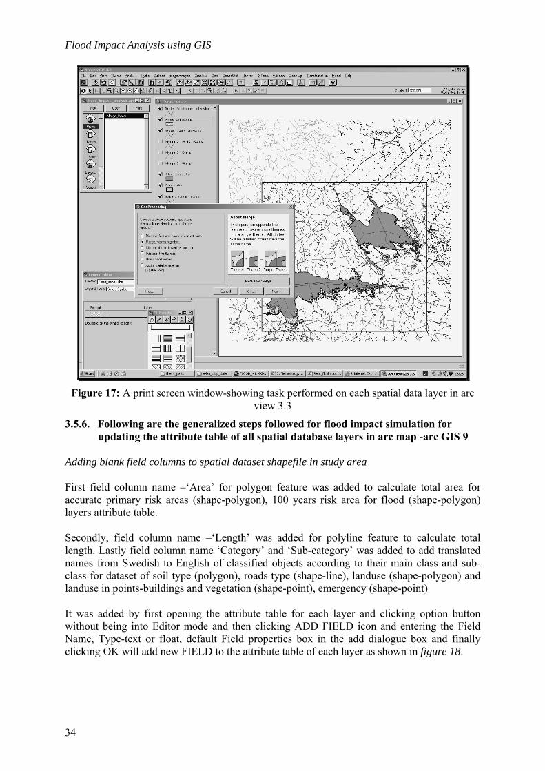
Flood Impact Analysis using GIS
Figure 17: A print screen window-showing task performed on each spatial data layer in arc
view 3.3
3.5.6. Following are the generalized steps followed for flood impact simulation for updating the attribute table of all spatial database layers in arc map -arc GIS 9
Adding blank field columns to spatial dataset shapefile in study area First field column name –‘Area’ for polygon feature was added to calculate total area for accurate primary risk areas (shape-polygon), 100 years risk area for flood (shape-polygon) layers attribute table. Secondly, field column name –‘Length’ was added for polyline feature to calculate total length. Lastly field column name ‘Category’ and ‘Sub-category’ was added to add translated names from Swedish to English of classified objects according to their main class and sub-class for dataset of soil type (polygon), roads type (shape-line), landuse (shape-polygon) and landuse in points-buildings and vegetation (shape-point), emergency (shape-point) It was added by first opening the attribute table for each layer and clicking option button without being into Editor mode and then clicking ADD FIELD icon and entering the Field Name, Type-text or float, default Field properties box in the add dialogue box and finally clicking OK will add new FIELD to the attribute table of each layer as shown in figure 18.
34

Chapter 3 Methodology
Figure 18: Adding blank field columns to spatial database layer in study area
Adding translated Swedish –English names in category and sub-category permanently for attribute table in each spatial dataset shapefile Adding of English translated names permanently in the attribute table was done in two steps. First in main data frame box, it was done by right clicking the layer to be edited and selecting joins and relates and clicking joins to open JOIN DATA dialogue box. In the join data box the join attributes from a table was selected from the dropdown list and further down in the box KKOD field was base to join English translation names to main attribute table and KKOD was selected in choose the field in this layer that the join will be based on & choose the field in the table to base the join on. The table prepared in excel for Swedish to English translation for the attributes table of all layer was choose in the table to join to this layer, or load the table from disk was selected. After clicking OK English translated names was added in a new field automatically as shown in figure 19.
Figure 19: Adding translated Swedish – English names in blank fields temporally for
working window
35

Flood Impact Analysis using GIS
Secondly as shown in figure 20 for adding permanent English translated names field in the attribute table, each layer attribute table was activated to open FIELD CALCULATOR dialogue box by right clicking newly added field columns to attribute table i.e. category and sub-category. In the field calculator dialogue box, FIELDS box the auto new temporary field generated for translated English names was selected to prepare permanent English names for category and sub-category for different dataset.
Figure 20: Adding translated Swedish –English names in blank fields for permanently in
attribute table
Calculating total area, length or count for each spatial dataset shapefile in study area Further to calculate total area, length or count of each spatial dataset in the study area namely accurate primary risk areas (shape-polygon), 100 years risk area for flood (shape-polygon) and flood prone areas (shape-polygon), soil type (polygon), roads type (shape-line), landuse (shape-polygon) and landuse in points-buildings and vegetation (shape-point) was done by being into editor mode for safer purpose, first attribute table of each theme was activated one by one and FIELD CALCULATOR dialogue was open by activating respective field-area or length to be calculated. In the FIELD CALCULATOR dialogue, the advanced button was checked as to enter the pre- logic VBA script code for area or length and area= as below to obtain the updated field with calculated area for each polygon and length for line as shown in figure 21. Pre- logic VBA script code for Area Dim dblArea as double Dim pArea as IArea Set pArea = [shape] dbl Area = pArea.area area = dblArea
36

Chapter 3 Methodology
Pre- logic VBA script code for Length Dim dblLength as double Dim pCurve as ICurve Set pCurve = [shape] dbl Length = pCurve.Length lenght = dblLength
Figure 21: Calculating total area, length or count for each spatial dataset layer in study area
Summarizing the attribute table for each spatial dataset shapefile in study area The summarizing for each spatial dataset layer namely accurate primary risk areas (shape-polygon), 100 years risk area for flood (shape-polygon), flood prone areas (shape-polygon), soil type (polygon), roads type (shape-line), landuse (shape-polygon), emergency (shape-point), landuse in points-buildings and vegetation (shape-point) was done being into editor mode for safer purpose. First attribute table of each theme was activated one by one and SUMMARIZE dialogue box was open by right clicking the respective field to be summarized viz. category or subcategory in the respective attribute table of layers and selecting a field in select a field to summarize box. Further choosing one or more summary statistics to be included in the output table box the length, area or count sum box was checked specifying output table path and finally clicking OK to obtain the desired result in dbf table file for the respective layer to be calculated as shown in figure 22.
37

Flood Impact Analysis using GIS
Figure 22: Summarizing the attribute table for each spatial dataset layer in study area
Exporting summarized dbf tables for each spatial dataset shapefile of study area into word format The summarized attribute table prepared for each layer into dbf format file as shown in figure 23 was opened with the help of Microsoft excel and the summarized table along with its calculated area or length or count with its classification was exported into report as shown in tables calculated for spatial data.
Figure 23: Exporting summarized dbf tables for each spatial dataset layer of study area into
word format
38

Chapter 3 Methodology
39
3.5.7. Pre-processing of data set for subset study area Lake Roxen and Lake Glan study area map
Figure 24: A map showing flood prone areas with study area i.e. total primary risk areas &
100 years risk area for flood along Lake Roxen and Lake Glan
Flood prone area Area in sq.m Area in sq.km Primary risk areas 26425910,25 26,43 100 years risk area for flood 32078524,70 32,09 Total flood prone areas 58504434,94 58,50
77300204,41 77,30 Lakes Lake Glan
Lake Roxen 95004100,72 95,00 Others water bodies 2690327,81 2,69
Table 4: A table showing calculated total area of different themes of study area in sq. m. and sq. km.

Flood Impact Analysis using GIS
Soil type map
Figure 25: A map showing clipped soil type with impact subset area
Soil type- % Total impact subset Area in [sq.km]
40%
2%23%
2%
2%
13%
18%0% Bare rock
Bog
Fine clay
Glaci fluvial
Gravels, sand
Lake
Morain
Morain clay
Figure 26: Pie diagram showing total percentage of soil type in impact subset area
40

Chapter 3 Methodology
41
Total impact subset area for Soil type
505,05
22,91
290,02
30,98 21,57
222,41
5,94
159,29
0
100
200
300
400
500
600
Bare rock Bog Fine clay Glacifluvial
Gravels,sand
Lake Morain Morainclay
Total Category
Tota
l Im
pact
are
a in
sq.
kmTotal impact subset area sq. km
Figure 27: Bar graph showing total sq. km. area of soil type in impact subset area
Impact area -Subset (frame) Category -Classified
Soil Type Total area in sq. m.
Total area in sq. km.
% Total area in sq. km.
Bare rock 505046394,23 505,05 40,14Bog 22905375,53 22,91 1,82Fine clay 290023272,27 290,02 23,05Glaci fluvial 30980983,65 30,98 2,46Gravels, sand 21574986,33 21,57 1,71Lake 159292199,66 159,29 12,66Morain 222410354,38 222,41 17,68Morain clay 5942857,96 5,94 0,47TOTAL 1258176424,01 1258,17 100,00
Table 5: A table showing calculated total clipped soil types area in sq. m. and sq.km.
The soil is sole means of support for all the terrestrial life. The productivity of soil is highly depended on the human and natural forces continuously acting upon it. The soil in the tropics areas can quickly lose their plant nutrients due to heavy rainfall and erosion. The soil can loose its original quality of nutrients if the waste from industrial and human are not treated properly. Lastly, with hydrosphere consider water flowing over the land surface in the form of sheet wash and streams (Jain et.al 1981). The top soil from agriculture land has a very high value of silt composition, which has good water holding capacity and productivity (Tahmina begum 1993). If this polluted soil nutrients mixed with the floodwater then it can create havoc. Above table, bar graph and pie diagram show total area of soil type in subset area. As shown in figures 26 and 27 the bare rock percentage is very high upto 40 % covering 505, 05 sq. km respectively. The Morain clay contributes almost negligible 0,47 % with only 5,94 % for having total area 5,94 sq km.The lake is also included in soil type as to understand that the lake floor is also affected when the flooding occurs.

Flood Impact Analysis using GIS
Landuse and Road type map The land use in flood plain has different uses like urban, industrial, agricultural and recreational uses or barren land. The changing scenario of landuse by human in today’s world that is responsible more for occurrence of flood then the hydrological activities (Hewitt 1997). It is likely to happen that urban area with clustered residential and industrial areas will bear more flood losses then the agriculture and recreational area.
Figure 28: A map showing clipped landuse type map and road network map with impact
subset area
42

Chapter 3 Methodology
Landuse- % Total impact subset Area in[sq.km]
23%
3%
1%
45%
0%
0%
0%
1%
2%
9%
1%
15%0%
0%
Area not surveyed
Arable land
Clear cut
Deciduous forest
Forest, coniferous and mixed
Group of buildings w ith courtyard
High-rise development
Industrial area
Leisure homes development
Low -rise development
Open area, diffuse transition
Other open land
Water w ith unclear shoreline
w ater
Figure 29: Pie diagram showing total percentage of landuse type in impact subset area
Landuse
0
288,14
32,99 9,72 0,07 1,63 5,52 3,75 14,66 23,51
113,78
6,38
194,38
563,66
0
100
200
300
400
500
600
Area
not
surv
eyed
Arab
le la
nd
Cle
ar c
ut
Dec
iduo
usfo
rest
Fore
st,
coni
fero
usan
d m
ixed
Gro
up o
fbu
ildin
gs w
ithco
urty
ard
Hig
h-ris
ede
velo
pmen
t
Indu
stria
l are
a
Leis
ure
hom
esde
velo
pmen
t
Low
-ris
ede
velo
pmen
t
Ope
n ar
ea,
diffu
setra
nsitio
n
Oth
er o
pen
land
Wat
er w
ithun
clea
rsh
orel
ine
wat
er
Total category
Tota
l Im
pact
are
a in
sq.
km
Total impact subset area sq. km
Figure 30: Bar graph showing total sq. km. area of landuse type in impact subset area
43

Flood Impact Analysis using GIS
44
Impact area -Subset (frame) Category -Classified Landuse type Total area
in sq. m Total area in sq. km
% Total area in sq. km
Arable land 288136727,69 288,14 22,90Area not surveyed 0,00 0,00 0Clear cut 32986822,12 32,99 2,62Deciduous forest 9719357,05 9,72 0,77Forest, coniferous and mixed 563663244,77 563,66 44,80Group of buildings with courty 67070,21 0,07 0,01High-rise development 1629875,07 1,63 0,13Industrial area 5515340,55 5,52 0,44Leisure homes development 3746504,32 3,75 0,30Low-rise development 14656978,75 14,66 1,17Open area, diffuse transition 23512106,40 23,51 1,87Other open land 113778798,98 113,78 9,04water 194375295,29 194,38 15,45Water with unclear shoreline 6382092,57 6,38 0,51
TOTAL 1258170213,77 1258,19 100,00
Table 6: A table showing calculated total clipped landuse types area in sq. m. and sq. km.
In above table bar graph and pie diagram landuse forest, coniferous and mixed category is 563, 66 sq km and is 40 % of total landuse subset area. Agriculture land is 288, 14 sq km that is contributing 22, 90 % of total subset area. The group of buildings with courtyard and high rise development is just too negligible under the impact subset area.
Road type-% Total impact subset Area in [km]
16%
53%
28%
3%
0%
other roads
private roads
public roads
railway
roads inunderpass
Figure 31: Pie diagram showing total percentage of road type in impact subset area

Chapter 3 Methodology
45
Road type
1555,18
802,41
4,27
454,97
87,34
0
200
400
600
800
1000
1200
1400
1600
1800
other roads private roads public roads railway roads in underpass
Total category
Tota
l Im
pact
are
a in
km
Total impact subset area km
Figure 32: Bar graph showing total km. area of road type in impact subset area
Impact area -Subset (frame) Category -Classified
Road type Total length
in m Total length
in km % Total length
in km
other roads 454965,2980 454,97 15,61
private roads 1555175,4180 1555,18 53,35
public roads 813080,3540 813,08 27,89
railway 87335,4290 87,34 3,00
roads in underpass 4273,9240 4,27 0,15
TOTAL 2914830,42 2914,83 100,00* List of further subcategories of category -classified road network in subset area is attached in appendix V-(a)
Table 7: A table showing calculated total clipped total road network length in m. and km.
In above table bar graph and pie diagram road type private roads has the highest network of 1555, 18 km with 53, 35% of the total roads and roads underpass is the least 4, 27 km with 0, 15 %. Also railway line is 87, 34 km with total 3% of the subset area connecting major towns.

Flood Impact Analysis using GIS
Landuse in points –buildings, hydrography, restriction and vegetation
Figure 33: A map showing clipped landuse in points-buildings, vegetation and hydrography
feature with impact subset area
Landuse in points-% Total impact subset Area in [count]
40%
1%
1%
58%
buildingdevelopment
hydrography
restriction
vegetation
Figure 34: Pie diagram showing total percentage of landuse in points in impact subset area
46

Chapter 3 Methodology
47
Landuse in points
0
1000
2000
3000
4000
5000
6000
7000
8000
9000
10000
building development hydrography restriction vegetation
Total category
tota
l im
pact
are
a in
cou
nt
Figure 35: Bar graph showing total count landuse in points in impact subset area
Impact area -Subset (frame) Category –Classified
Landuse in points Total count % Total count
building development 6046 40,20
hydrography 180 1,20
restriction 201 1,34
vegetation 8611 57,26
TOTAL 15038 100,00* List of further subcategories of category-classified landuse in points is attached in appendix V-(b)
Emergency-fire station 1
Table 8: A table showing calculated total counts of clipped classified landuse in points-buildings, vegetation and hydrography features
In above table bar graph and pie diagram of landuse in points vegetation count are the highest having total count 8611 with 57,26 % of the total subset area, followed by building development 6046 total count with 40,20 % and the hydrography and restriction feature are very less with 180 and 201 total count with 1,20 % and 134 % respectively.

Flood Impact Analysis using GIS
3.5.8. Following was the final task for flood impact analysis map products in arc map -arc GIS 9
Carrying out spatial overlay analysis for all the landuse shapefile data with flood risk shapefile data Lastly all the clipped layer with frame namely soil type (shape-polygon), roads type (shape-line), landuse (shape-polygon), emergency (shape-point), landuse in points-buildings and vegetation (shape-point) were finally analyzed together with accurate primary risk areas (shape-polygon), 100 years risk area for flood (shape-polygon) in Arc Map -Arc GIS 9. Using overlay analysis tool for flood impact analysis viz. map and tables are the end products for the affected road type, soil type, landuse, emergency, landuse in points-building and vegetation in flood prone area in and around Lake Roxen and Lake Glan as shown in figures 36,39,42 and 45; and table 10,11,12 and 13 respectively.
48

Chapter 4 Results and analysis
Chapter 4.
4.1.
Results and analysis
Flood impact analysis and map products Following is the description of which types of analysis has been performed and which types of map products can be derived in GIS for informed flood hazard management. 4.1.1. Identification of endangered areas For town planning and floodplain management, there is need to map various hazard zones as a means for setting development guidelines and establishing emergency response procedures. Mapping of flood extents have obvious uses in showing area affected by a particular historical flood or a modeled flood of a given probability of occurrence. Once the possible flood levels have been derived, maps for each flood level can be effortlessly produced with GIS. GIS tools can readily perform different landuse based overlay analysis in planning context. It can also produce maps of resultant analysis. When overlaid on property or an infrastructure database, it can be analyzed which property or infrastructure is immediately at risk. Visual representation can definitely add value to the results of the numerical impact analysis for informed planning and hazard management. Figure 21 shows example of flood hazard map with primary risk areas and 100 years risk area for flood. Figures 35, 38, 41 and 44 respectively show soil type, road type, landuse, landuse in points-Buildings and Vegetation spatial data selected by an overlay analysis. 4.1.2. Impact analysis for the affected landuse, road network, soil type and landuse in
points feature Overlay analysis between landuse, vegetation, road type, buildings, soil type and extent of the flood prone areas can be identified vulnerable areas to environmental, socio-economic damage. Figures and calculated tables below show flood impact on each spatial dataset in subset area. It could be very well observed that emergency services have been planned and located in a flood hazard proof area. These kinds of impact analysis maps can also provide necessary inputs during land use planning exercises. The maximum extent calculated for flood prone area is less then 6 km from the edges of the lake.
49

Flood Impact Analysis using GIS
Affected Landuse:
Figure 36: A map showing affected landuse type along the study area
Landuse- % Total impact area in [sq. Km]
0%
48%
0%5%12%
0%
0%
0%
1%
0%
11%
19%
0%
4%
Area not surveyed Arable landClear cutDeciduous forestForest, coniferous and mixedGroup of buildings with courtyardHigh-rise developmentIndustrial areaLeisure homes developmentLow-rise developmentOpen area, diffuse transitionOther open landWater with unclear shorelinewater
Figure 37: Pie diagram showing total percentage of affected landuse type in impact area
50
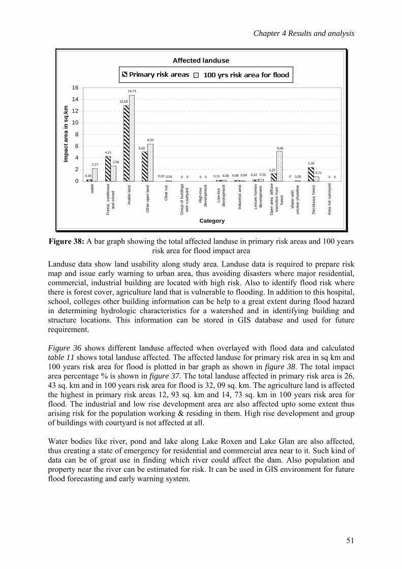
Chapter 4 Results and analysis
Affected landuse
4,21
0 0
2,34
0
2,17
14,73
6,34
0,04 0 0 0,05 00
1,220,220,080,130,02
5,02
12,93
0,260,710,310,040,08
2,56
5,06
0
2
4
6
8
10
12
14
16w
ater
Fore
st, c
onife
rous
and
mix
ed
Ara
ble
land
Oth
er o
pen
land
Cle
ar c
ut
Gro
up o
f bui
ldin
gsw
ith c
ourty
ard
Hig
h-ris
ede
velo
pmen
t
Low
-rise
deve
lopm
ent
Indu
stria
l are
a
Leis
ure
hom
esde
velo
pmen
t
Ope
n ar
ea, d
iffus
etra
nsiti
on fr
omfo
rest
Wat
er w
ithun
clea
r sho
relin
e
Dec
iduo
us fo
rest
Are
a no
t sur
veye
d
Category
Impa
ct a
rea
in s
q.km
Risk Area Sq. Km Flooded area Sq. Km
Figure 38: A bar graph showing the total affected landuse in primary risk areas and 100 years
risk area for flood impact area
Landuse data show land usability along study area. Landuse data is required to prepare risk map and issue early warning to urban area, thus avoiding disasters where major residential, commercial, industrial building are located with high risk. Also to identify flood risk where there is forest cover, agriculture land that is vulnerable to flooding. In addition to this hospital, school, colleges other building information can be help to a great extent during flood hazard in determining hydrologic characteristics for a watershed and in identifying building and structure locations. This information can be stored in GIS database and used for future requirement. Figure 36 shows different landuse affected when overlayed with flood data and calculated table 11 shows total landuse affected. The affected landuse for primary risk area in sq km and 100 years risk area for flood is plotted in bar graph as shown in figure 38. The total impact area percentage % is shown in figure 37. The total landuse affected in primary risk area is 26, 43 sq. km and in 100 years risk area for flood is 32, 09 sq. km. The agriculture land is affected the highest in primary risk areas 12, 93 sq. km and 14, 73 sq. km in 100 years risk area for flood. The industrial and low rise development area are also affected upto some extent thus arising risk for the population working & residing in them. High rise development and group of buildings with courtyard is not affected at all. Water bodies like river, pond and lake along Lake Roxen and Lake Glan are also affected, thus creating a state of emergency for residential and commercial area near to it. Such kind of data can be of great use in finding which river could affect the dam. Also population and property near the river can be estimated for risk. It can be used in GIS environment for future flood forecasting and early warning system.
51

Flood Impact Analysis using GIS
Affected Road type:
Figure 39: A map showing affected road type along the study area
Road type -% Total impact area in [km]
14%
54%
26%
6% 0%
other roads
private roads
public roads
railway
roads inunderpass
Figure 40: Pie diagram showing total percentage of affected road type in impact area
52
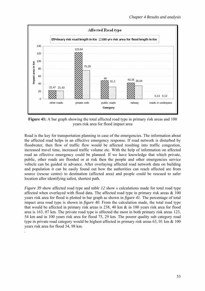
Chapter 4 Results and analysis
Affected Road network
Risk road length in Km Flooded road length Km
22,47
123,54
43,26
0,13 0,12
49
75,29
35,0431,2
21,43
0
20
40
60
80
100
120
140
other roads private rods public roads railway roads in underpass
Category
Impa
ct a
rea
in k
m
Figure 41: A bar graph showing the total affected road type in primary risk areas and 100
years risk area for flood impact area
Road is the key for transportation planning in case of the emergencies. The information about the affected road helps in an effective emergency response. If road network is disturbed by floodwater, then flow of traffic flow would be affected resulting into traffic congestion, increased travel time, increased traffic volume etc. With the help of information on affected road an effective emergency could be planned. If we have knowledge that which private, public, other roads are flooded or at risk then the people and other emergencies service vehicle can be guided in advance. After overlaying affected road network data on building and population it can be easily found out how the authorities can reach affected are from source (rescue centre) to destination (affected area) and people could be rescued to safer location after identifying safest, shortest path. Figure 39 show affected road type and table 12 show s calculations made for total road type affected when overlayed with flood data. The affected road type in primary risk areas & 100 years risk area for flood is plotted in bar graph as shown in figure 41. The percentage of total impact area road type is shown in figure 40. From the calculation made, the total road type that would be affected in primary risk areas is 238, 40 km & in 100 years risk area for flood area is 163, 07 km. The private road type is affected the most in both primary risk areas 123, 54 km and in 100 years risk area for flood 75, 29 km. The poorer quality sub category road type in private road category would be highest affected in primary risk areas 63, 01 km & 100 years risk area for flood 34, 98 km. .
53
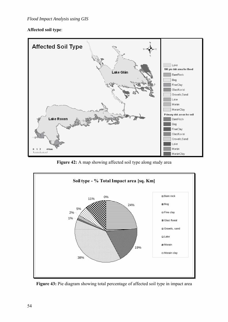
Flood Impact Analysis using GIS
Affected soil type:
Figure 42: A map showing affected soil type along study area
Soil type - % Total Impact area [sq. Km]
24%
19%
38%
1%
2%5%
11% 0% Bare rock
Bog
Fine clay
Glaci fluvial
Gravels, sand
Lake
Morain
Morain clay
Figure 43: Pie diagram showing total percentage of affected soil type in impact area
54

Chapter 4 Results and analysis
Affected Soil Type
6,23
8,69
0,32
3,49
0,65
5,96
0,02
7,62
14,08
0,11 0,29
2,01
0,031,07
4,95
2,99
0
2
4
6
8
10
12
14
16B
areR
ock
Fine
Cla
y
Gla
ciflu
vial
Mor
ain
Gra
vels
,San
d
Lake
Bog
Mor
ain
Cla
y
Category
Impa
ct a
rea
in s
q.km
Risk Area Sq. Km Flooded area Sq. Km
Figure 44: A bar graph showing the total affected soil type in primary risk areas and 100
years risk area for flood impact area
To understand which buildings are most likely to sustain damage, the rescue team needs to have latest information about affected soil type. Also to know what soils could be contaminated, eroded and lose fertility while the actual occurrence of flood. The figure 42 and Table 11 shows the calculated affected soil type that could be risk to building. The affected area in sq. km at primary risk areas and 100 years risk area for flood is plotted in bar graph as shown in figure 44. The total impact area percentage % is shown in figure 43. The total soil type that would be affected in primary risk areas is 26,43sq km in 100 years risk area for flood is 32,08sq km. From the calculation made the fine clay soil type would be affected the most both in primary risk areas 8, 69 sq. km and in 100 years risk area for flood 14, 08 sq. km. When flood occurs the erosional activities are to its peak, there is large amount of soil nutrients loss, pesticides from agriculture field, and industrial waste that gets deposited in lake along with the flood water.
55

Flood Impact Analysis using GIS
Affected landuse in points:
Figure 45: A map showing affected landuse in points along the study area
Landuse in points - % Total impact area in [count]
30%
2%
1%67%
building development
hydrography
restriction
vegetation
Figure 46: Pie diagram showing total percentage of affected landuse in points in impact area
56

Chapter 4 Results and analysis
Affected Landmark
Risk count Flooded count
10 3
141
9
382
170
8
319
0
50
100
150
200
250
300
350
400
450
buildingdevelopment
hydrography restriction vegetation
Category
Impa
ct a
rea
in c
ount
Figure 47: A bar graph showing total affected landuse in points in primary risk areas and 100
years risk area for flood impact area
Buildings and demographic data can be co-related together as each building represents some population staying there. Further this data can be of utilized in GIS for preparing hazards map to identify the population that resides in the primary risk areas and needs to be warned and evacuated first. The high density population can be at more risk during emergency as there can be huge loss of life, therefore there is need to plan how this people moves to safer place. This kind of risk data can be also be useful for insurance and real estates agencies. There are total 565 parcels identified along the Lake Roxen and Lake Glan. Out of these 137 commercial and residential buildings lie in the in 100 years risk area for flood and 164 commercial and residential buildings are in primary risk areas. The affected area is shown in figure 45 and the calculated area affected is shown in table 13. The affected count in primary risk areas and 100 years risk area for flood is plotted in bar graph as shown in figure 47 The total impact count percentage % is shown in figure 46 The total counts calculated for landuse in points-vegetation and buildings, monuments etc that would be affected in primary risk areas is 565 and in 100 years risk area for flood is 477, 00.
57

Flood Impact Analysis using GIS
58
4.1.3. Calculated tables for impact area Tables 9, 10,11 12, 13, 14, 15 and 16 below are the results of the spatial overlay and tabular analysis performed in GIS using spatial functions and relational database concepts in Arc Map- Arc GIS 9.
Flood Prone Areas
Risk Area45%
Flooded area55%
Figure 48: Pie diagram showing total percentage of affected flood prone area in impact area
Below table 9 shows calculations for flood prone areas, water bodies and digitized layers of lake areas as shown in figure 23 from the pdf maps from SMHI and Räddningsverket report for Motala Ström River. Also in the legend of pdf report there exist two flood prone areas classes, one calculated risk class I for dams which are identified as PRIMARY RISK AREAS and second flood prone areas according to calculation based on 100 years statistics of water flow identified as 100 YEARS RISK AREA FOR FLOOD in this thesis write-up.
Flood prone area type
Flood area in sq.m
Flood area in sq. km
Percentage of area in sq. km (%)
Primary risk areas
26425910,25 26,43 45,2
100 years risk area for flood
32078524,70 32,09 54,8
Total Flood prone areas
58504434,94 58,50 100
77300204,41 77,30Lakes: Lake Glan Lake Roxen
95004100,72 95,00
Others water bodies
2690327,81 2,69
Table 9: A table showing total calculated flood prone area and other water bodies in sq. m, sq.km and percentage

Chapter 4 Results and analysis
59
Affected landuse:
IMPACT AREA KKOD CATEGORY- LANDUSE Primary risk
area in sq. m.100 years
risk area for flood in sq.
m.
Primary risk
area in sq. km
100 yrs risk area for flood in sq. km
% Primary risk area
km
% 100 years
risk area for flood
km
Total Impact area in sq. km
% Total Impact area in sq. km
% Total impact Area / subset area
4 Arable land 12933691,60 14728364,54 12,93 14,73 48,92 45,90 27,66 47,27 2,20 20 Area not surveyed 0,00 0,00 0,00 0,00 0,00 0,00 0,00 0,00 0,00
6 Clear cut 17434,12 38634,15 0,02 0,04 0,08 0,12 0,06 0,10 0,00 19 Deciduous forest 2341238,23 707360,17 2,34 0,71 8,85 2,21 3,05 5,21 0,24
2 Forest, coniferous and mixed
4206404,26 2564093,32 4,21 2,56 15,93 7,98 6,77 11,57 0,54
12 Group of bldg. with courtyard
0,00 0,00 0,00 0,00 0,00 0,00 0,00 0,00 0,00
13 High-rise development
0,00 0,00 0,00 0,00 0,00 0,00 0,00 0,00 0,00
15 Industrial area 82652,26 36529,96 0,08 0,04 0,30 0,12 0,12 0,21 0,01 16 Leisure homes
development 221325,95 310234,93 0,22 0,31 0,83 0,97 0,53 0,91 0,04
14 Low-rise develop. 126693,51 82002,65 0,13 0,08 0,49 0,25 0,21 0,36 0,02 17 Open area, diffuse
transition from forest
1220404,00 5064734,01 1,22 5,06 4,62 15,77 6,28 10,73 0,50
5 Other open land 5015338,85 6335375,11 5,02 6,34 18,99 19,76 11,36 19,41 0,90 1 Water 259290,87 2165897,95 0,26 2,17 0,98 6,76 2,43 4,15 0,19
18 Water with unclear shoreline
1435,55 45330,42 0,00 0,05 0,00 0,16 0,05 0,09 0,00
TOTAL 26425909,20 32078557,21 26,43 32,09 100,00 100,00 58,52 100,00 4,65
Table 10: A table showing total affected landuse shapefile in primary risk areas and 100 years risk area for flood calculated in sq.m and sq. km

Flood Impact Analysis using GIS
60 Affected soil type:
IMPACT AREA JORD_ID CATEGORY-SOIL TYPE Primary
risk area in sq. m.
100 years risk area
for flood in sq. m.
Primary risk area in sq. km
100 years risk area for flood in sq. km
% Primary risk area sq. km
% 100 years risk area for flood sq.
km
Total impact area in sq. km
% Total impact area in sq. km
% Total impact Area / subset area
7 BareRock 6226360,32 7621887,67 6,23 7,62 23,57 23,75 13,85 23,67 1,10
1 Bog 5958554,23 4949410,01 5,96 4,95 22,55 15,43 10,91 18,65 0,87
2 FineClay 8693871,41 14077346,62 8,69 14,08 32,88 43,89 22,77 38,92 1,81
4 Glacifluvial 322047,83 108350,46 0,32 0,11 1,21 0,34 0,43 0,73 0,03
3 Gravels, Sand 645813,63 288059,98 0,65 0,29 2,46 0,90 0,94 1,61 0,07
10 Lake 1071933,92 2009926,92 1,07 2,01 4,05 6,27 3,08 5,26 0,24
6 Morõn 3488317,12 2990243,71 3,49 2,99 13,20 9,32 6,48 11,08 0,52
5 MorõnClay 19010,70 33331,85 0,02 0,03 0,08 0,09 0,05 0,09 0,00
TOTAL 26425909,16 32078557,22 26,43 32,08 100,00 100,00 58,51 100,00 4,65
Table 11: A table showing total affected soil type shapefile in primary risk areas and 100 years risk area for flood calculated in sq.m and sq. km

Chapter 4 Results and analysis
61
Affected road type:
IMPACT AREA Sr. No.
CATEGORY-ROAD TYPE Primary
risk for length in
m
100 years risk area for flood length in
m
Primary risk for
length in km
100 years risk area for flood length in
km
% Primary
risk length km
% 100 years risk area for
flood length km
Total impact
lenght in km
% Total impact
lenght in km
% Total impact lenght / subset area
1 other roads 22465,15 21429,75 22,47 21,43 9,42 13,14 15,61 14,43 0,54
2 private roads 123536,10 75293,35 123,54 75,29 51,82 46,17 58,05 53,67 2,00
3 public roads 49003,93 31197,76 49,00 31,20 20,56 19,13 27,96 25,85 0,96
4 railway 43260,86 35036,61 43,26 35,04 18,15 21,49 6,4 5,92 0,22
5 roads in underpass 133,21 117,18 0,13 0,12 0,06 0,07 0,14 0,13 0,00
TOTAL 238399,24 163074,66 238,40 163,07 100,00 100,00 108,16 100,00 3,72 * List of further subcategories of category –classified for affected road type in impact area is attached in appendix V-(c)
Table 12: A table showing total affected road type shapefile in primary risk areas and 100 years risk area for flood calculated in m and km

Flood Impact Analysis using GIS
62 Affected landuse in points:
IMPACT AREA Sr. No.
CATEGORY- LANDUSE IN POINTS No. of parcel
affected: Primary risk
count
No. of parcel affected: 100 years
risk area for flood count
% of parcel affected:
Primary risk count
% of parcel affected: 100 years risk area for flood
count
Total impact area
in count
% Total impact area
in count
% Total impact count /
subset area
1. building development 170 141 30,09 29,56 311 29,85 2,07
2. hydrography 10 9 1,77 1,89 19 1,82 0,13
3 restriction 3 8 0,53 1,68 11 1,06 0,07
4 vegetation 382 319 67,61 66,88 701 67,27 4,66
TOTAL 565 477 100,00 100,00 1042 100,00 6,93 * List of further subcategories of category-classified for affected landuse in points in impact area is attached in appendix V-(d)
Table 13: A table showing total number of parcel affected for landuse in points shapefile in primary risk areas and 100 years risk area for flood

Chapter 4 Results and analysis
4.2. Significance of flood impact analysis: The response system based on GIS can perform the impact analysis and help to alert the emergency response system of the nearby administration. The following analysis shows some of the procedures that can be performed using the system. 4.2.1. Property data linking The effectiveness of emergency response depends on awareness and preparedness for flood hazard within the community. As shown in figure 49 affected property owners could be educated with the possible flood hazard and be first contacted and evacuated in case of any emergency. In addition, historic flood levels for each property could be stored which definitely could serve as a base to gauge future flood predictions.
OID
Street level
Gatan Street
Figure 49: OID in landuse theme could be use to link the affected parcel forresponse planning
Once the analysis has been performed and parcel affected by the flood have bthe database could be linked to various spatial dataset using the object ID (OIDthe property at risk in landuse in points theme. Assessment of property valuatioassessment of the damage can be precisely calculated. The percentage area property could be calculated with overlay analysis and be linked to propedatabase. Once linked, total tangible damage can be assessed. 4.2.2. Emergency planning A call comes to desk of emergency response chief about the vulnerable areaevacuation. The area is at high risk of getting flooded and there need forvulnerable population and movable property. The police, fire and rescue departa GIS based evacuation procedure to cope with real emergencies. Assumemergency situation occurs as shown in figure 50. The population staying in uneeds to be evacuated is shown in figure 50. The fire department and other agbe prepared to deal with a flooding state of emergencies.
Risk level
emergency
een identified, ) \ KKOD for n or economic
of the affected rty assessment
that needs an evacuation of ment could use ing a state of rban areas that encies need to
63

Flood Impact Analysis using GIS
Figure 50: A print screen window showing evacuation planning for emergencies for shortest
path
Fire rescue team, police officer, together with social services agencies is asked to start rescue operation. After receiving report from the metrological department, they would demarcate flood prone areas on available GIS administrative map. The emergency response team first put the early warning out in radio, TV, internet, phones and the best possible methods to be reach-out to an individual residing the demarcated risk areas. Simultaneously send messages to the hospital and other agencies to be prepare for the state of emergencies. Police is asked to stop further penetrating of local people into demarcated flood prone areas. For assessing flood risk to propose evacuation plan there needs to be administrative data i.e. maps with administrative details especially with local street names and address ranges inside the evacuation areas, critical care facilities needing special attention, such as hospitals or nursing homes and safer sites at higher elevation. Apart from administrative data, there is need of demographic, topographic data with good road-network connectivity details, and flood details. All spatial data with the help of spatial analysis tools can be overlayed in ArcGIS with one another and the desired nearest healthcare facilities, school, safer location and evacuation routes, building and population residing into that building, streets at risk could be obtained and provided to rescue team to carry out the evacuation safely and quickly. From the above the spatial data, different required data can be identified required during flood emergency for planning mass evacuation. From administrative data of kommune that intersect with flood prone areas, mass evacuation plan could be obtained to rescue people and their properties.
64

Chapter 4 Results and analysis
4.2.3. Landfill
Figure 51: Affected landuse and soil type due to landfill selected by overlay analysis using
orthophoto image
65

Flood Impact Analysis using GIS
The landfill is hazardous waste disposal from urban and rural areas from residential and industrial areas. There are lots of environmental problems caused if this point source and non-point source pollution areas are flooded. The emission of various gases (methane), toxic organic substances, nutrient releases causes damage to vegetation, crops, soil, contamination of ground water and surface water finally affecting human and environment. When overlaying landfill sites with soil and landuse impact area shown in figure 51. It was identified that most of landfill sites intersecting the impact area were situated in the southwest part of Lake Roxen in an open land area near bank of river. If these areas are flooded then there is severe impact to surrounding environment. The fine clay soil type, river water and landuse area upto some extent could be potential threat. 4.2.4. Sharing risk data with public It will allow non-technical users to analyze how infrastructure like schools, hospitals, water, road, landuse etc. would be affected in flood hazard zones. A person can wisely decide if his property will be at risk or in establishing up of new infrastructure, he could identify safer location (Mitchell 1998; Lang 2001). A resident can use spatial data to overlay schools data with flood hazard zone and find out if his children school is located in flood prone areas and built up on loosely compacted soil, making it a high-risk structure. He further can contact the school administration and shares emergency route information with his family (Mitchell 1998; Lang 2001). A business organization can use this data to map his employee homes, potential emergency shelter and other employers that can be guided by providing evacuation plan (Mitchell 1998; Lang 2001). A nearby hospital, the application is used by GIS analyst to estimate how many patients to expect after flood occurrence. Further this application can be enhanced by adding the time of occurrence of flood, in case if it is night then the number of people affected will be more (Mitchell 1998; Lang 2001).
66

Chapter 4 Results and analysis
67
Effects of impact analysis on dataset: Major = > 25 % of total impact area Minor < 25 % of total impact area
Type of dataset None Minor Major Landuse Agriculture √ Forest √ Residential areas √ Commercial areas √ Recreational areas √ Infrastructure √ Others √ Landuse in points Restriction √ Building development √ Vegetation √ Hydrography √ Soil type BareRock √ FineClay √ Glacifluvial √ Moraine √ Gravels, Sand √ Bog √ Moraine Clay √ Water bodies River √ Lake √ Transportation Network Public roads √ Private roads √ Roads in underpass √ Other roads √ Railways √ Landforms floodplains
√
Table 14: Impact analysis table for different dataset

Flood Impact Analysis using GIS
Table 14 shows summarization of the effects of flood impact analysis on different dataset. Depending upon the impact area the dataset type was grouped in three categories i.e. if the dataset is not at all under impact then it is classified under ‘None’ category, if the total area is less than 25% then it is classified under ‘Minor’ category and lastly if the total impact area is more then or equal to 25 % then it is classified under ‘Major' category.
In landuse dataset types from the analysis made, agriculture area would be under maximum impact then residential, commercial, recreational, infrastructure and other types. In landuse in points dataset types the maximum impact would be observed in building developments then the restriction, vegetation and hydrography features. In soil type the fine clay soil type would have the maximum impact then the other bare rock, fine clay, glaci-fluvial, moraine, gravel, sand, bog and moraine clay type.
In the transportation network public and private roads shows the major impact area then roads underpass, other roads and railways.
68

Chapter 5 Discussion and conclusion
Chapter 5.
5.1.
5.2.
Discussion and conclusion
Discussion The studies made by (Sivertun and Eriksson 1992) for calculation of nitrogen and phosphorous in Bornsjön catchment area. It refers from figures obtained from nature protection department, that total phosphorus leached in 1983 in open land is 0, 2 kg\ha.year, forest is 0, 07 kg\ha.year, urban areas is 0, 3 kg\ha.year and in lake is 0, 05 kg\ha.year. Similarly, for nitrogen leached into the open land are 13 kg\ha.year, forest 1, 9 kg\ha.year, and urban areas 5 kg\ha.year and in lake is 10 kg\ha.year. The data from Länsstyrelsen 1989 depicts value 0, 1 to 0, 3 animals \ hectare adds 0, 2 kg\ha phosphorous and nitrogen 8 kg\ha. Similarly values 0, 5 to 1, 1 releases 0, 5 - 2, 4 kg \ ha and 14 -22 kg \ ha respectively. In Lake Roxen, deposition of phosphorus is estimated to be 1000 tons from 1950.In studies made by Chaiwanakupt and Robertson in 1976 it states that 650 kg \ ha phosphrous is stored in land area over a period of 20 years and that has resulted into 8500 kg \ ha storage of total phosphrous in land area. If this leached nitrogen and phosphorous when mixes with the floodwater, it can cause lot of adverse effects to human health and environment. One of the possible solution could be, empty reservoir from time to time so as to avoid the risk for flood and accumulation of nutrients in reservoir and lake. If there is flooding situation around Lake Roxen and Lake Glan it will severely damage its surrounding environment, first of all it will rise the water level around its periphery, due to this the nutrient deposited or stored in ground will suddenly come up and dissolve with the flood water increasing the possible threats to the surrounding. The water level of the Lake Roxen and Lake Glan should be controlled properly with the controlling of gates. If huge amount of floodwater containing pollutants percolate into water then it will not only contaminate the soil but also the non-pollutated ground water. Especially the water level should be controlled around the Lake Roxen and Lake Glan from increasing, by controlling the floodgates, constructing the dams.
Conclusion The ESRI Arc Map- Arc GIS 9 and Arc View 3.3 GIS software used to prepare data, integrate and analyze data. The spatial dataset for landuse, road network, soil type and landuse in points were integrated to analyze in GIS. All this spatial dataset is needed while planning for flood emergency. It was found that landuse, road and soil was affected more or less upto some extent when the areas along Lake Roxen and Lake Glan are flooded. This information can be used for planning an effective flood emergency response in flood-inundated area using GIS. The flood impact analysis can be used to obtain information about the population, property, and environment at risk during occurrence of flood in a specific area. The emergency response department can use GIS in case of flooding to find out which street, school, hospital needs to be evacuated. The GIS can calculate the total number of residents within the area, so as to prepare an effective evacuation plan which can be utilized by different rescue agencies.
69
Flood Impact Analysis using GIS
Based on the simple queries for population and building constructed on the primary risk areas and 100 years risk area for flood can be identified and with this information, the administration or authority can meet with buildings owners and other people in locality to initiate an effective disaster preparedness programs Command centre for flood forecasting: The flood mitigation is major task but with flood impact analysis, the estimated loss of environment can be identified and mitigated upto some extent with the proper use of emergency planning using GIS. Jointly structural and non-structural measures with use of GIS technology can immensely help flood command centre. Also it helps different kommune at administrative level, engineering agencies, NGO and other agencies to take appropriate measures during actual occurrence of flood. Proper land use planning in flood prone areas from evacuating point of view can be done, by prohibiting further encroachment of residential and industrial zones in high-risk areas, but only allowing open activities like setting up of playground or parks. Flood risk maps: Identification of flood hazard zone and preparation of GIS based flood impact maps will help authorities for quick assessment during occurrence of disaster. Thus, GIS data base should be developed for the decision makers, planners to take positive steps in case of emergency with the previous data available. Flood rescue system: Using object ID or KKOD for identifying different property or landuse at risk and road network data in the flood hazard zone can be used to generate location spatial dataset of different location and routes. Using this spatial dataset in network analyst (a special GIS tool), the best route in different situation to go from one location to another could be found out. This kind of analysis could also help giving early warning to people, for guiding them in which direction they should travel, secondly during disaster the rescue team needs to reach the victim and disaster location, and lastly the victim needs to be taken immediately to hospital or other relief camps. 5.3. Further studies The further studies can be done with use of orthophoto and digital elevation model (DEM) for the study area, by creating 1m contours interval while keeping base contour 33 m at lake water level and find out how much landuse, road etc would be affected for each interval in flood prone areas zones. Secondly, with the help of DEM and other topographic information the amount toxic elements, nutrients flow into Lake Roxen and Lake Glan can be calculated. Such kind of information can be of great use for authorities when planning emergency, particularly for small region and environmental studies respectively. Also by overlaying flood prone areas with ortho photo, interpretation can be made to improve river channel and further construction of embankment on rivers flowing in to Lake Roxen and Lake Glan. Using different raster and vector data set 3-dimensional flood modelling can be made to provide a visualization effects for actual occurrence of flood and impact of inundation of landuse features.
70
References
References
Research papers, articles & books
Alkema, D. (2004): RS & GIS application in Flood forecasting, International Institute for Geo-Information Science and Earth Observation webpage, http://www.itc.nl/library/Papers_2004/n_p_conf/alkema.pdf (acc.2004-10-10)
Andersson, L. & Arheimer B. (2003): ‘Modelling of human and climatic impact on nitrogen load in a Swedish river 1885–1994’, Hydrobiologia, vol. 497, pp. 63-77
Arheimer, B. and Brandt, M. (1998): ‘Modelling nitrogen transport and retention in the catchments of southern Sweden’. Ambio, vol. 27, no.6
Aziz F., Tripathi N., Ole, M. & Kusanagi, M. (2002): Development of flood warning system, GIS development webpage, http://www.gisdevelopment.net/ application /natural_hazards/ floods/nhcy0005a.htm (acc.2004-10-11)
Bernhardsen, T. (1999): Geographic Information Systems, an Introduction (Second edition) Wiley: New York
Bertilsson, S. & Widenfalk, A. (2002): ‘Photochemical degradation of PAHs in freshwaters and their impact on bacterial growth – influence of water chemistry’, Hydrobiologia, vol. 469, pp. 23-32
Black, A. R. (1996): ‘Major flooding and increased flood frequency in Scotland since 1988’. Physics and Chemistry of the Earth, 20(5-6), pp. 463-468
Blomqvist, G. (2003): Patterns of chloride deposition next to a road as influenced by salting occasions and winds, Transportation Research Board (TRB) Annual Meeting CD-ROM Paper Number 03-3760, http://www.ltrc.lsu.edu/TRB_82/TRB2003-001760.pdf (acc.2005-04-24)
Brivio, P. A., Colombo, R., Maggi, M. & Tomasoni, R. (2002): ‘Integration of remote sensing data & GIS for accurate mapping of flooded area’, International Journal of Remote Sensing, vol. 23, no. 3, pp. 429–441
Burrough, P.A. (1986): Principles of Geographical Information System for earth Resources Assessment, Clarendon Press: Oxford
Chorley, R. J. (1978): Introduction to Geographical Hydrology, Methuen and Company Ltd: New York
Congalton R. & Green K. (1992): ‘The ABCs of GIS: An introduction to geographic information systems’, Journal of Forestry, vol. 90, no. 11, pp. 13-20
Cova T. J. & Church R. L. (1997): ‘Modelling community evacuation vulnerability using GIS’, International Journal of Geographical Information Science, 11(8), pp. 763-784
Dombrowsky, W.R. (1995): ‘Again & Again: Is a Disaster What We Call a ‘Disaster? Some Conceptual Notes on Conceptualising the Object of Disaster Sociology’, Internal Journal of Mass Emergencies and Disasters, vol. 13, no. 3, pp. 241-254
71
Flood Impact Analysis using GIS
Edwards, M. M. (2002): Development Impact Analysis, Program on Agricultural Technology studies (PATS) webpage, http://www.pats.wisc.edu/pdf%20documents/CommDev.pdf (2005-06-13)
EM-DAT (2005): ‘The OFDA / CRED International Disaster Database: 06 www.em-dat.net - Université Catholique de Louvain - Brussels – Belgium’, Created on: Jun-28-2005 - Data version: v05
Eriksson, T. (2004): Variations in bioavailability of dissolved organic matter during a spring flood episode in northern Sweden, Swedish University of Agricultural Sciences, Department of Forest Ecology, Graduate Thesis in Soil Science
Eriksson, S. & Sivertun (1992): ‘Calculation of transport of Nitrogen and Phosphorous by using satellite images and GIS’ Lund, Vatten, vol.48, pp 117-127
Fogelberg, S. (2003): Modelling Nitrogen Retention at the Catchment scale: Comparison between HBV-N and MONERIS, Report Uppsala tekniska högskola, UPTEC W 03 019 Uppsala University: Uppsala
Gebeyehu, A. (1989): Regional Flood frequency analysis, Hydraulics laboratory, the royal institute of technology Stockholm, Sweden
Geological Society of London –GSL (2001): The Earth in Our Hands; Flooding http://www.geolsoc.org.uk/pdfs/floods_aw.pdf (acc.2004-06-23)
Gierke, J. S. (2002): Engineering Applications in the Earth Sciences: River Velocity, Michigan Technical University, Michigan Tech webpage, http://www.cee.mtu.edu/peacecorps/documents_november_02/use_of_manning_equation_for_measuring_river_velocity.pdf (acc.2004-10-15)
Goodchild, M.F. (1993): The state of GIS for Environmental Problem Solving, in - Goodchild, M.F., Parks, B. and Steyaert, L. (Eds), Environmental modelling with GIS, Oxford University Press, New York, USA, pp. 147–167
Gopalakrishnan, M.: Forecasting & warning system for an effective disaster preparedness & response, Central Water Commission presentation, UNDP webpage, www.undp.org.in /UNDMT/dpm/ Day%20One/Theme%20I%20Presentation/GK.ppt (acc.2004-10-12)
Gupta, A. (2000): Information technology and natural disaster management in India, GIS@ development webpage, http://www.gisdevelopment.net/aars/acrs/2000/ts8/hami0001.shtml (acc.04-10-24), GIS@development, India
Häggström, M., Lindström, G., Cobos, C., Martfnez, J., Merlos, L., Monzo, R.D., Castillo, G., Sirias, C., Miranda, D., Granados, J., A1faro, R., Robles, E., Rodrfguez, M. & Moscote, R. (1990): Application of the HBV model for flood forecasting in six Central American rivers. SMHI Hydrology, No. 27, Norrköping
Håkan, S. (1994): Application of the HBV model to the upper Indus River for inflow forecasting to the Tarbela Dam, SMHI Hydrology, No.48, Norrköping
Hall, J. W.; Meadowcroft, I. C., Sayers, P. B. & Bramley, M. E. (2003): ‘Integrated Flood Risk Management in England and Wales’, Natural Hazards Rev., vol. 4,no. 3, pp. 126-135
72

References
73
Herath, S. (2001): ‘Geographical Information Systems in Disaster Reduction, Information Technology for Disaster Management’, ADRC International Paper, Tokyo: Japan, No.1 pp. 25-31
Hewitt, K. (1997): Regions of risk, A geographical introduction to disasters, Longman, Ltd: Essex, U.K.
Heywood, I., Cornelius, S. and Carver, S. (2002): An Introduction to Geographical Information System, IInd edition, Pearson Education: Harlow
Houston, S. & MacFarlane, B. (2000): ‘Natural Hazards and Hurricane Evacuation Planning with GIS’, Colorado State University webpage, http://www.cnr.colostate.edu/avprojects/00proj/hurr_haz/web_docs/ProjDesc.html (2005-04-16)
Hoyois, P. and Guha - Sapir, D. (2005): ‘Flood Disasters in Europe’ - a Short Analysis of EM – DAT International Disaster Database for Years 1985 – 2004’, CRED, Université Catholique de Louvain, Belgium
Hursley Parish Council Flood Plan (2003): Hampshire County Council webpage, http://www.hants.gov.uk/parish/hursley/hursleyfloodplan.htm (2005-04-26)
Hydrologiska Byråns Vattenbalansavdelning (HBV) (2004): Swedish Metrological and Hydrological Institute, SMHI webpage, http://www.smhi.se/foretag /m/hbv_ demo/html / welcome.html (acc. 04-06-21)
Jain, R.K., Urban, L. V. and Stacey, G. S. (1981): Environmental Impact Analysis: A new dimension in decision- making, IInd edition, Van Nostrand Reinhold Co: New York
Jalaluddin, Md. A. H. (2001): ‘Integration of 3s and Mathematical Modelling in Disaster Management in Bangladesh’, Surface Water Modelling Centre Dhaka, Bangladesh http://www.bytesforall.org/8th/DMBSeminar.PDF (acc. 2005-04-15)
Jiang, M. (2003): GIS and Hydrological Modeling for Flood control; Final Thesis - Linköpings universitet. Institutionen för datavetenskap- IDA, Linköpings
Karlsson, G. (1989): Dynamics of Nutrients mass transport–A river basin evaluation, Linköping studies in arts and science 40, Linköpings
Kates R. W (1965) Industrial Flood Losses: Damage Estimation in Lehigh Valley, Chicago: University of Chicago, Department of Geography, Paper no. 98
Kraijenhoff, D.A. and Moll, J.R. (1986): River flow modelling and forecasting, Water Science and Technology Library, Reidel, Dordrecht, Netherlands
Lang, L. (2001): Managing Natural resources with GIS, ESRI press: California
Laudon, H. (1999): Spring flood pH decline in Northern Sweden - Towards an operational model separating natural acidity from anthropogenic acidification, Swedish University of Agricultural Sciences: Umeå

Flood Impact Analysis using GIS
74
Laurini, R. & Thompson, D. (1992): Fundamentals of Spatial Information systems, no. 37, in The A.P.I.C. Series, Academic Press: New York
Lavakare, A. (1997): GIS & Risk Assessment, GIS@development webpage, http://www.gisdevelopment.net/application/miscellaneous/misc010a.htm (acc.2004-04-10) GIS@development, India
Lehner, B., Henrichs, T., Döll, P., Alcamo, J. (2001): EuroWasser — Model-based assessment of European water resources and hydrology in the face of global change, Kassel World Water Series 5, Center for Environmental Systems Research, University of Kassel, Germany, 130 pp. http://www.usf.uni- kassel.de/usf/archiv/dokumente.de.htm (acc. 2005-06-21
Lindström, G. and Alexandersson, H. (2004): ‘Recent Mild and Wet Years in Relation to Long Observation Records and Future Climate Change in Sweden’, AMBIO, a journal of the human environment, vol. 33, no. 4, pp. 183–186
Liu, J., Wei, C., Li, Y. and Yin, Z. (1999): ‘Application of GIS in Flood Control of Government Agencies’, The Proceedings of Geoinformatics'99 Conference, Ann Arbor, Michigan, pp. 1-6
Lundqvist, A. (2003): The Liming in Northern Sweden- the administrative handling of the scientific Disputes, Bachelor of Science Thesis, Linköpings universitet. Department of thematic studies, Norrköping
Maidment, D. R. (1993): GIS and hydrological modelling in Goodchild M.F., Parks B. and Steyaert L., Editors, Environmental modelling with GIS, Oxford University Press: New York, pp. 147–167
Massam, B.H. (1980): Spatial Search: Application to planning problems in the public sector, Pergamon: Oxford
McHarg, I. L. (1969): Design with nature, Natural History Press: New York
Milbrink, G., Timm, T. and Lundberg, S. (2002): ‘Indicative profundal oligochaete assemblages in selected small Swedish lakes’, Hydrobiologia, vol. 468, no. 1 - 3, pp. 53 - 61
Mitchell, A. (1998): ‘Zeroing in: Geographic information system at work in the community’, ESRI press: California
Montoya, L. (2003): ‘Geo-data acquisition through mobile GIS and digital video: an urban disaster management perspective’, Environmental Modelling & Software, volume 18, no. 10, pp. 869-876
Moore, D. (2002): GIS in Emergency Planning -A Spatial Analysis of Ambulance Services, Spatial Planning solution web page, http://www.spatial.ie (2004-11-12)
Morin, M., Jenvald, J. and Thorstensson, M. (2000): ‘Computer-supported visualization of rescue operations’, Safety Science, vol. 35, no. 1-3, pp. 3-27

References
Nawaz, F., Shafique, M. (2003): Data integration for flood risk analysis by using GIS/RS as tools, GIS@development webpage, http://www.gisdevelopment.net/application /natural_ hazards/floods/ma03032c.htm, (acc.2004-10-11) GIS@development, India
Newson, M. D (1975): Flooding and flood hazards in the United kingdom, Oxford University Press: London
Nirupama, (2002): ‘Role of remote sensing in disaster management’, ICLR Research Paper Series – No. 21, Institute for Catastrophic Loss Reduction - ICLR webpage, http://www .iclr.org/pdf/Niru_report%20Simonovic.pdf (acc. 2004-04-21)
Pine J. C. (1999): ‘Geographic Information System in Emergency Management. From Technology and Emergency Management’, Session from a course prepared for the Federal Emergency Management Agency, Washington, D.C. Plate, E. J. (2002): ‘Flood risk and flood management’, Journal of Hydrology, vol. 267, no. 1-2, pp. 2-11
Project Roxen \ Glan (1992): Roxen och Glan –Vattenmiljö, mål och åtgärder; Finspångs, Linköpings och Norrköpings kommuner Länsstyrelsen I Östergötlands län, : Länsstyr. Linköping
Räddningsverket, (2001): ‘Översiktlig översvämningskartering längs Motala ström, Sträckan från Vättern till Bråviken Projekt’, Översiktlig översvämningskartering Rapport, no. 17
Rau, J. G. and Wooten, D. C. (1980): Environmental Impact Analysis handbook, McGraw-Hill: New York
Rego, A. J. (2001): ‘National Disaster Management Information Systems & Networks: An Asian Overview’, Global Disaster Information Network (GDIN) conference, Asian Disaster Preparedness Centre webpage, http://www.adpc.net/infores /adpc-documents/paperatgdin01 .pdf (acc. 04-09-27)
Reinelt, L. (1990): Nonpoint Source Water Pollution Management. Monitoring, Assessment and Wetland Treatment – Linköping: Linköpings Universitet, 155 s., Linköping studies in arts and science; No. 57, Avhandling vid Tema Vatten
Reinelt, L., Sivertun, Å. and Castensson, R. (1989): ‘A GIS to target critical areas for non-point source management’, Proceedings of the International Source Management Symposium, Austin, Texas
Relief web (2004): Flash Flood North-Western states, UN Developmental programme, Relief web webpage, http://www.reliefweb.int/w/rwb.nsf/unid/2a02222 (acc.2004-09-12)
Sanyal, J. and Lu, X. X. (2003): Application of GIS in flood hazard mapping: A case study of Gangetic West Bengal - India, GIS@development webpage, http://www. gisdevelopment.net /application/natural_hazards/floods/ma03138a.htm (acc.2004-10-11) GIS@development, India
Savenije H. H. G., Cunnane, C. and Demaree, G. R. (1996): Recent extreme floods in EU and US flood prone areas: what’s in the future? Physics and chemistry of the earth, Pergamon : Oxford
75

Flood Impact Analysis using GIS
76
Sharma, V. K. (2003): Use of GIS related technologies for managing disasters in India: an overview, GIS@development webpage, http://www.gisdevelopment.net/application/natural_ hazards/overview/nho0003.htm (acc.04-09-12) GIS@development, India
Sinnakaudan, S., Ghani, A. A., Ahmad, S. S. and Zakaria, N. A. (2003): ‘Flood risk mapping for Pari River incorporating sediment transport’, Environmental Modelling & Software, vol. 18, no. 2, pp. 119-130
Sivertun, A. (1993): Geographical Information Systems as a Tool for Analysis and Communication of Complex Data diss., Geographical reports no 10, Department of Geography, Umea Universitet: Umeå
Sivertun, A. (1993): Geographical Information System (GIS) as a tool for analysis and communication of Multidimensional data, Department of Geography (0366) Umeå Universitet: Umeå
Star, J. and Estes, J. (1990): Geographic Information system: An Introduction, Englewoods Cliffs, Prentice Hall: New Jersey
Sue S. (1998): Delineation of a Flood Evacuation Route for Mustang Island- TX, Center for research in water resources (CRWR) webpage, http://www.crwr.utexas.edu/gis/gishydro99/class/sue/pro.htm (2005-05-09)
Sui, D. Z. and Maggio, R. C. (1999): ‘Integrating GIS with hydrological modelling: practices, problems, and prospects’, Computers, Environment and Urban Systems, vol. 23, no.1, pp. 33-51
Tahmina, B. (1993): ‘The Impact of a flood control embankment on the soil, agriculture and socio-economy, a case study of the Pathakhali -konai project in Bangladesh’, department of Physical Geography, Uppsala Universitet: Uppsala
Thielen, J., Roo, A. D., Gouweleeuw, B. and Schmuck, G. (2001): ‘Application of Medium-Range Weather Forecasting on Pre-Flood Warning Simulations on European Scale’, European Conference on Application in Meteorology
Trnka, J. (2002): Hazmat Transportation Accidents: Introducing GIS as a core Information System in Emergency management, Final Thesis - Linköpings universitet. Institutionen för datavetenskap- IDA, Linköpings
United Nations Environment Programme, UNEP, (2002): ‘Early Warning, Forecasting and Operational Flood Risk Monitoring in Asia -Bangladesh, China and India’ – Proceedings of the Project Workshop (GT/1010-00-04): UNEP/GRID Sioux Falls, EROS Data Center, Sioux Falls, SD, USA
United Nation, UN (2003): ‘Guidelines on participatory planning and management for flood mitigation and preparedness’, ix, 129 s.: ill., Water resources series, 0082-8130, no. 82, United Nations: New York
United Nations Environment Programme, UNEP: EIA Training Resource Manual IInd edition (2002): Impact Analysis, Chapter 6 - UNEP webpage, http://www.unep.ch/etu/publications/EIA_2ed/EIA_E_top6_body.PDF (2005-05-23)
References
Vedin, H., Eklund, A. and Alexandersson, H. (1999): The rainstorm and flash flood at Mount Fulufjället in August 1997: The meteorological and hydrological situation, Geogr. Ann. 81 A, pp. 361-368
Wessel, J. (1996): ‘Institutional frameworks for flood management’, Annales geophysicae, pp. 310
Willén, T. and Mattsson, R. (1997): ‘Water-blooming and toxin-producing cyanobacteria in Swedish fresh and bracish waters, 1981–1995’, Hydrobiologia, vol. 353, no. 1-3, pp. 181-192(12), Kluwer Academic
World Bank, (1989): ‘Bangladesh Action Plan for Flood Control’, Washington D.C., Asian Region Country Department I, World Bank
World Bank, (1990): ‘Flood Control in Bangladesh; A Plan for Action’, World Bank Technical Paper number 119, Asia Region Technical Department
Yang, X. (2001): Predicting flood inundation and risk using geographic information system and hydrodynamic model: a technical report on the case study at Eskilstuna, Gävle GIS Institute, University of Gävle. Sweden
Zerger, A. and Smith, D. I. (2003): ‘Impediments to using GIS for real-time disaster decision support’, Computers, Environment and Urban Systems, vol. 27, no. 2, pp. 123-141
Zhang, J., Xul, K., Watanabe, M., Yang, Y. and Chen, X. (2004): ‘Estimation of river discharge from non-trapezoidal open channel using QuickBird-2 satellite imagery’, Hydrological Sciences–Journal, 49(2)
77

Flood Impact Analysis using GIS
Electronic sources 01. Ambulance van image: Antares webpage, http://www.antares.co.uk/images/ambulance.jpg (2005-05-12) 02. Flood image: King county webpage, http://dnr.metrokc.gov/dnrp/press/2004/img/Nov90-snoq-flood-lg.jpg (2005-05-12) 03. GIS Command centre image: Fuse webpage, “photos”, http://fuse.pha.jhu.edu/photos/general/SCC.GIF (2005-05-12) 04. Hospital image: Michele Maki's webpage, http://michelesworld.net/dmm2/lulu/municipa/hospital.jpg (2005-05-12) 05. Helicopter Ambulance Image: The delta dragon webpage, http://www.cantho-rvn.org/craft/Air-Ambulance-J-Jones-550x281.jpg (2005-05-12) 06. Mobile phone image: Wireless developer network webpage, http://www.wirelessdevnet.com/channels/lbs/geomode2/geomode2a.jpg (2005-05-12)
78

Appendixes
Appendixes
Appendix 1. Internet electronic resources: 1. http://www.gis.com 2. http://www.infodirekt.se 3. http://www-lexikon.nada.kth.se/skolverket/swe-eng.shtml 4. http://dictionary.reference.com 5. http://www.bibl.liu.se 6. http://www.geo.ed.ac.uk/agidict/welcome.html(AGI online GIS dictionary) 7. http://support.esri.com/index.cfm?fa=knowledgebase.gisDictionary.browse&letter 8. http://ESRI GIS dictionary 9. http://gislounge.com 10. http://en.wikipedia.org/wiki/Main_Page 11. http://www.sciencedirect.com 12. http://www.google.se/ and http://scholar.google.com 13. http://www.linkoping.se/index.htm 14. http://www.norrkoping.se 15. http://www.scb.se 16. http://www.e.lst.se/e/amnen/Krishantering/ 17. http://www.gisdevelopment.net 18. http://www.lm.se/kartplan/index.htm 19. http://www.srv.se 20. http://www3.interscience.wiley.com/cgi-bin/home 21. http://ambio.allenpress.com/ambioonline/?request=search-simple
Appendix 2. Questionnaire – verbal interview with personnel
1. Does your organization know and use Geographic Information system (GIS) in case of emergencies?
2. What are the different types of emergencies? 3. How do you response to an emergency situation? 4. Do you have any static plans to overcome any emergency flood situation? 5. Do you have any problem in dealing with emergencies specifically with flooding
situation and using GIS? 6. What kind of information, maps and data does your organization use in case of
emergencies? 7. What is the accuracy, scale data do you use in case of emergency? 8. What is the software that you use for emergency analysis? 9. What kind of problems you overcome while using different spatial GIS data in case of
emergencies? 10. Do you use stored GIS database created for the past emergencies to monitor and have
real time emergency situation? Thankyou Organization: Place: Contact person: Date and time:
79

Flood Impact Analysis using GIS
Appendix 3. List of persons consulted for information
1. Barbro Näslund - Landenmark Swedish Rescue Services Agency ,
2. Bodil karlsson - Swedish Rescue Services Agency, [email protected]
3. Hans Eriksson - Norrköping Fire and rescue service- Brandförsvar, [email protected]
4. Jonas Sjölin - Chef GIS-enheten Norrköpings kommune, [email protected]
5. Sören Almgren - Lantmäteriet, [email protected]
6. Bo Holst - Swedish metrological Hydrological Institute- SMHI [email protected]
7. Lindström Göran - Swedish Metrological and Hydrological Institute, SMHI [email protected]
8. Sanner Håkan - Swedish Metrological and Hydrological Institute, SMHI, [email protected]
9. Yacoub Tahsin - Swedish Metrological and Hydrological Institute, SMHI [email protected]
Appendix 4. Common file format
1. Dbase: database files
2. TIFF: Tag image file format- Desk top publishing format
3. Shapefile: ESRI Arc view format
Appendix 5. Formula for calculation
Total affected area classification –wise, for various flood prone areas.
1. Percentage affected area = (Affected area/total area) * 100
2. Affected shapefile layer = shapefile layer <INTERSECT/CLIPPED> flood prone areas (features that overlap in the themes were restored in the output cover).
3. Conversion of sq.m to sq. km = X sq m/1000000=Y sq. km
4. Calculation of percentage % = Total X/Total Y*100= Total X, Y %
80

Appendixes
81
Appendix 6. List of further subcategories of category-classified for road network and landuse in points table
(a) * List of further subcategories of category -classified road network type in subset area:
Impact area -Subset (frame) Category -classified Road type
Sub-category Total
length in m
Total length in
km
% Total length in
km other roads Footpath 209915,70 209,92 7,20other roads Hiking trail - coinciding
with other road 1033,97 1,03 0,04
other roads Hiking trail - footpath 2836,82 2,84 0,10other roads Illuminated skining /
jogging track 28445,49 28,45 0,98
other roads Road in park, cycle path 17786,46 17,79 0,61other roads Tractor track 194946,87 194,95 6,69private roads Approach road 136784,67 136,78 4,69private roads Better quality road 41512,99 41,51 1,42private roads Poorer quality road 608154,18 608,15 20,86private roads Road 768723,58 768,72 26,37public roads Major street 47732,58 47,73 1,64public roads Motorway 43950,37 43,95 1,51public roads Road 5 - 7 m wide 142047,41 142,05 4,87public roads Road < 5 m wide 154547,52 154,55 5,30public roads Road > 7 m wide 89691,66 89,69 3,08public roads Roads under
construction 10671,70 10,67 0,37
public roads Street 251567,53 251,57 8,63public roads Street within closed
group of buildings 1742,65 1,74 0,06
public roads Street within closed group of buildings, Entry
19346,68 19,35 0,66
public roads Through traffic 51782,26 51,78 1,78railway Closed railway line
(rails removed) 8976,36 8,98 0,31
railway Industrial track, historic railway line
8513,01 8,51 0,29
railway Standard gauge, double track, electrified
43060,00 43,06 1,48
railway Standard gauge, single track, electrified
1067,68 1,07 0,04
railway Standard gauge, single track, not electrified
25718,38 25,72 0,88
roads in underpass Better quality road, underpass
46,57 0,05 0,00
roads in underpass Major street, underpass 284,14 0,28 0,01roads in underpass Motorway, underpass 625,30 0,63 0,02

Flood Impact Analysis using GIS
82
roads in underpass Poorer quality, underpass
79,62 0,08 0,00
roads in underpass Road 5 - 7 m wide, underpass
363,82 0,36 0,01
roads in underpass Road > 7 m wide, underpass
253,54 0,25 0,01
roads in underpass Road, underpass 724,22 0,72 0,02roads in underpass Street within group of
buildings, underpass, Entry
330,95 0,33 0,01
roads in underpass Street, underpass 73,98 0,07 0,00roads in underpass Through road,
underpass 173,00 0,17 0,01
roads in underpass Underpass railway and tramway
1013,23 1,01 0,03
roads in underpass Underpass, other roads and tracks
305,56 0,31 0,01
TOTAL 291483,42 2914,83 100,00
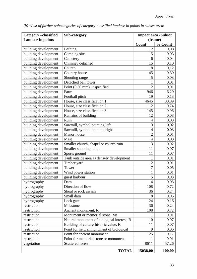
Appendixes
83
(b) *List of further subcategories of category-classified landuse in points in subset area:
Impact area -Subset (frame)
Category –classified Landuse in points
Sub-category
Count % Count building development Bathing 12 0,08building development Camping site 5 0,03building development Cemetery 6 0,04building development Chimney detached 15 0,10building development Church 18 0,12building development Country house 45 0,30building development Shooting range 5 0,03building development Detached bell tower 1 0,01building development Point (0,30 mm) unspecified 2 0,01building development Farm 946 6,29building development Football pitch 19 0,13building development House, size classification 1 4645 30,89building development House, size classification 2 112 0,74building development House, size classification 3 145 0,96building development Remains of building 12 0,08building development Ruin 4 0,03building development Sawmill, symbol pointing left 3 0,02building development Sawmill, symbol pointing right 4 0,03building development Manor house 2 0,01building development Mast 4 0,03building development Smaller church, chapel or church ruin 3 0,02building development Smaller shooting range 11 0,07building development Sports ground 11 0,07building development Tank outside area as densely development 1 0,01building development Timber yard 2 0,01building development Tower 7 0,05building development Wind power station 1 0,01building development guest harbour 5 0,03hydrography Dam 4 0,03hydrography Direction of flow 108 0,72hydrography Shoal or rock awash 36 0,24hydrography Small dam 8 0,05hydrography Lock gate 24 0,16restriction Milestone 36 0,24restriction Ancient monument, R 108 0,72restriction Monument or memorial stone, Ms 1 0,01restriction Natural monument of biological interest, B 10 0,07restriction Building of culture-historic value, K 11 0,07restriction Point for natural monument of biological 9 0,06restriction Point for ancient monument 25 0,17restriction Point for memorial stone or monument 1 0,01vegetation Scattered forest 8611 57,26
TOTAL 15038,00 100,00

Flood Impact Analysis using GIS
84 (c) *List of further subcategories of category –classified for affected road type in impact area:
IMPACT AREA KKOD CATEGORY-ROAD TYPE
SUB-CATEGORY Primary risk for
flood length in m
100 years risk area for flood length
in m
Primary risk for flood
length in km
100 years risk area for flood length
in km
% Primary risk for flood
length km
% 100 years risk area for flood length
km 264 other roads Footpath 2931,63 5562,07 2,93 5,56 1,23 3,41
5098 other roads Road in park \ cycle path 1840,33 2866,25 1,84 2,87 0,77 1,76 5095 other roads Tractor track 17693,20 13001,43 17,69 13,00 7,42 7,97 265 other roads Hiking trail - footpath 0,00 0,00 0,00 0,00 0,00 0,00 266 other roads Illuminated skining /
jogging track 0,00 0,00 0,00 0,00 0,00 0,00
268 other roads Hiking trail - coinciding with other road
0,00 0,00 0,00 0,00 0,00 0,00
5091 private roads Approach road 7333,42 3477,44 7,33 3,48 3,08 2,13 5061 private roads Better quality road 5132,59 2742,53 5,13 2,74 2,15 1,68 5082 private roads Poorer quality road 48063,03 34977,30 48,06 34,98 20,16 21,45 5071 private roads Road 63007,06 34096,08 63,01 34,10 26,43 20,91 5051 public roads Major street 528,23 875,59 0,53 0,88 0,22 0,54 5011 public roads Motorway 8987,61 4022,18 8,99 4,02 3,77 2,47 5025 public roads Road 5 - 7 m wide 8796,68 5825,07 8,80 5,83 3,69 3,57 5029 public roads Road < 5 m wide 8444,95 4164,90 8,44 4,16 3,54 2,55 5022 public roads Road > 7 m wide 9903,65 7246,26 9,90 7,25 4,15 4,44 5056 public roads Street 9916,85 7372,87 9,92 7,37 4,16 4,52 5034 public roads Street within closed group
of buildings, Entry & exit roads (ramps) at junction, Class 3
1389,51 917,18 1,39 0,92 0,58 0,56
5044 public roads Through traffic 1036,45 773,71 1,04 0,77 0,43 0,47 5014 public roads Roads under construction 0,00 0,00 0,00 0,00 0,00 0,00

Appendixes
85
5033 public roads Street within closed group of buildings, Entry & exit roads (ramps) at junction, Class 2
0,00 0,00 0,00 0,00 0,00 0,00
5058 public roads Street within closed group of buildings, Entry & exit roads (ramps) at junction
0,00 0,00 0,00 0,00 0,00 0,00
273 railway Standard gauge, double track, electrified
20953,72 17494,20 20,95 17,49 8,79 10,73
271 railway Standard gauge, single track, not electrified
22307,14 17542,41 22,31 17,54 9,36 10,76
272 railway Standard gauge, single track, electrified
0,00 0,00 0,00 0,00 0,00 0,00
278 railway Closed railway line (rails removed)
0,00 0,00 0,00 0,00 0,00 0,00
279 railway Industrial track, historic railway line
0,00 0,00 0,00 0,00 0,00 0,00
5811 roads in underpass
Motorway, underpass 78,29 00,00 0,08 00,00 0,03 00,00
5871 roads in underpass
Road, underpass 54,92 117,18 0,05 0,12 0,02 0,07
286 roads in underpass
Underpass railway and tramway
0,00 0,00 0,00 0,00 0,00 0,00
5822 roads in underpass
Road > 7 m wide, underpass
0,00 0,00 0,00 0,00 0,00 0,00
5825 roads in underpass
Road 5 - 7 m wide, underpass
0,00 0,00 0,00 0,00 0,00 0,00
5834 roads in underpass
Street within group of buildings, underpass Entry & exit roads (ramps) at interchange, Class 3, underpass
0,00 0,00 0,00 0,00 0,00 0,00

Flood Impact Analysis using GIS
86 5844 roads in underpass
Through road, underpass 0,00 0,00 0,00 0,00 0,00 0,00
5851 roads in underpass
Major street, underpass 0,00 0,00 0,00 0,00 0,00 0,00
5856 roads in underpass
Street, underpass 0,00 0,00 0,00 0,00 0,00 0,00
5861 roads in underpass
Better quality road, underpass
0,00 0,00 0,00 0,00 0,00 0,00
5882 roads in underpass
Poorer quality, underpass 0,00 0,00 0,00 0,00 0,00 0,00
5899 roads in underpass
Underpass, other roads and tracks
0,00 0,00 0,00 0,00 0,00 0,00
TOTAL 238399,24 163074,66 238,40 163,07 100,00 100,00

Appendixes
87
(d) *List of further subcategories of category-classified for affected landuse in points in impact area:
IMPACT AREA KKOD CATEGORY- LANDUSE IN POINTS
SUB-CATEGORY No. of parcel
affected: Primary risk
count
No. of parcel affected: 100 years risk for flood count
% of parcel affected:
Primary risk count
% of parcel affected:100 years risk for flood count
362 building development Guest harbour 1 2 0,18 0,42 373 building development Mast 0 0 0,00 0,00 731 building development Farm 14 6 2,48 1,26 732 building development Country house 4 0 0,71 0,00 733 building development House, size classification 3, 2 0 0,35 0,00 735 building development House, size classification 1, 141 128 24,96 26,83 736 building development House, size classification 2, 4 2 0,71 0,42 737 building development Manor house 0 0 0,00 0,00 739 building development Tank outside area 0 0 0,00 0,00 740 building development Sawmill, symbol pointing left 0 0 0,00 0,00 741 building development Church 0 0 0,00 0,00 746 building development Ruin 0 0 0,00 0,00 747 building development Smaller chapel \ church ruin 0 0 0,00 0,00 748 building development Detached bell tower, symbol 0 0 0,00 0,00 749 building development Point (0,30 mm) unspecified 0 2 0,00 0,42 754 building development Timber yard 0 0 0,00 0,00 755 building development Sawmill, symbol pointing right 1 0 0,18 0,00 756 building development Wind power station 0 1 0,00 0,21 757 building development Chimney detached 0 0 0,00 0,00 759 building development Tower 1 0 0,18 0,00

Flood Impact Analysis using GIS
88 762 building development Cemetery 0 0 0,00 0,00 763 building development Sports ground 1 0 0,18 0,00 766 building development Football pitch 1 0 0,18 0,00 767 building development Shooting range 0 0 0,00 0,00 768 building development Smaller shooting range 0 0 0,00 0,00 774 building development Remains of building 0 0 0,00 0,00 777 building development Bathing 0 0 0,00 0,00 778 building development Camping site 0 0 0,00 0,00 369 hydrography Lock gate 3 1 0,53 0,21 511 hydrography Direction of flow 7 7 1,24 1,47 522 hydrography Shoal or rock awash 0 0 0,00 0,00 525 hydrography Small dam 0 0 0,00 0,00 526 hydrography Dam 0 1 0,00 0,21 341 restriction Milestone 1 1 0,18 0,21 773 restriction Ancient monument R 1 2 0,18 0,42 781 restriction Natural monument of bio. interest 0 1 0,00 0,21 783 restriction Building of culture-historic value 1 0 0,18 0,00 784 restriction Monument or memorial stone, Ms 0 1 0,00 0,21 785 restriction Natural monument of geo. interest 0 1 0,00 0,21 786 restriction Point for ancient monument 0 1 0,00 0,21 787 restriction Monument or memorial stone 0 1 0,00 0,21 451 vegetation Scattered forest 382 319 67,61 66,88
TOTAL 565 477 100 100
***

Datum Date
Language
English
Report category
Licentiatavhandling
Examensarbete
C-uppsats
D-uppsats
Övrig rapport
ISBN
ISRN LIU-IDA-D20--05/016--SE
Serietitel och serienummer ISSN Title of series, numbering
Avdelning, institution Division, department
Institutionen för datavetenskap
Department of Computer and Information Science 8
Linköpings universitet
URL för
http:/
Title:
Author:
Floo
Vim
Abstrac
Floodsdeterioi.e. strwhich and otplanniflood dspatialplan anis to aalong also psystem Using and Laareas adata pbe an maker
Keywor
Analys(GIS),overla
elektronisk version:
/urn.kb.se/resolve?urn=urn:nbn:se:liu:diva-4206
d Impact Analysis using GIS: A case stud
alkumar A. Vaghani
t:
are common natural disaster occurring in most parration of environment. There have been immense uucturally and non-structurally. Undoubtedly, structinvolves physical work like construction of dams, rher embankments to keep floods away from peopng like flood forecasting and warning, flood plain amage to keep people away from floods. Thus, non
information on maps with high accuracy in less ti effective emergency response towards flood disaste
nalyze impact of flood in the flood prone areas. Ththe demarcated flood prone areas of Lake Roxen anroposes how to use current flood information duri. This provides spatial information for area in the flo
map overlay analysis in GIS software (ArcGIS); floke Glan was digitize from PDF maps. Thus, the thlong Lake Roxen and Lake Glan are flooded. ESRI
reparation, integrating, analyzing, and spatial data weffective tool for development of flood emergency ss.
ds:
is, Data set, Decision-maker, Digitized, Disaster, En Georeferenced, Hazard zone, Impact , Lake Roxen ay analysis, Sweden, Emergency, Vulnerable.
2005-06-0
y for Lake Roxen and Lake Glan-Sweden
ts of the world. This results in damage to human life and ses of technology to mitigate measures of flood disaster ural measures are very expensive and time consuming eservoirs, bridges, channel improvement, river diversion le. Whereas non-structural measures is concerned with zoning, relief and rehabilitation for reducing the risk of -structural measures involve analysis, planning providing me. Non-structural measures can help decision maker to r. A one of the good way to plan non-structural measures e thesis tries to analyze impact of flood on environment d Lake Glan in Östergötland County, Sweden. The thesis ng flood emergency utilizing geographical information od zone for assessment regarding flood vulnerability.
od prone areas and topographic data along Lake Roxen esis work is an effort to analyze impact of flood when
® GIS software Arc Map 9 and Arc View 3.3 is used for ith attribute table information. Finally, to show GIS can ystem as a part of disaster preparedness by the decision
vironment, Flood, Geographical information system nd Lake Glan, Remote Sensing, Risk, River, Spatial

På svenska Detta dokument hålls tillgängligt på Internet – eller dess framtida ersättare – under en längre tid från publiceringsdatum under förutsättning att inga extra-ordinära omständigheter uppstår.
Tillgång till dokumentet innebär tillstånd för var och en att läsa, ladda ner, skriva ut enstaka kopior för enskilt bruk och att använda det oförändrat för ickekommersiell forskning och för undervisning. Överföring av upphovsrätten vid en senare tidpunkt kan inte upphäva detta tillstånd. All annan användning av dokumentet kräver upphovsmannens medgivande. För att garantera äktheten, säkerheten och tillgängligheten finns det lösningar av teknisk och administrativ art.
Upphovsmannens ideella rätt innefattar rätt att bli nämnd som upphovsman i den omfattning som god sed kräver vid användning av dokumentet på ovan beskrivna sätt samt skydd mot att dokumentet ändras eller presenteras i sådan form eller i sådant sammanhang som är kränkande för upphovsmannens litterära eller konstnärliga anseende eller egenart.
För ytterligare information om Linköping University Electronic Press se förlagets hemsida http://www.ep.liu.se/ In English The publishers will keep this document online on the Internet - or its possible replacement - for a considerable time from the date of publication barring exceptional circumstances.
The online availability of the document implies a permanent permission for anyone to read, to download, to print out single copies for your own use and to use it unchanged for any non-commercial research and educational purpose. Subsequent transfers of copyright cannot revoke this permission. All other uses of the document are conditional on the consent of the copyright owner. The publisher has taken technical and administrative measures to assure authenticity, security and accessibility.
According to intellectual property law the author has the right to be mentioned when his/her work is accessed as described above and to be protected against infringement.
For additional information about the Linköping University Electronic Press and its procedures for publication and for assurance of document integrity, please refer to its WWW home page: http://www.ep.liu.se/
Copyright © 2005 by Vimalkumar A. Vaghani, Linköping