FLOOD FREQUENCY AND STORM RUNOFF OF URBAN … · flood frequency and storm runoff of urban areas of memphis and shelby county, tennessee ... iv . flood frequency

WATER RESOURCES INVESTIGATIONS REPORT 84-4 110

FLOOD FREQUENCY AND STORM RUNOFF OF URBAN AREAS OF MEMPHIS AND

SHELBY COUNTY, TENNESSEE

Prepared by

U.S. GEOLOGICAL SURVEY

in cooperation with the

CITY OF MEMPHIS AND SHELBY COUNTY, TENNESSEE

http://www.usgs.gov

njestes

Click here to return to USGS publications

../index.html

FLOOD FREQUENCY AND STORM RUNOFF OF URBAN AREAS

OF MEMPHIS AND SHELBY COUNTY, TENNESSEE Braxtel L. Neely, Jr.

U.S. GEOLOGICAL SURVEY

Water-Resources Investigations Report 84-4 110

Prepared in cooperation with the

CITY OF MEMPHIS and SHELBY COUNTY,

TENNESSEE

Memphis, Tennessee 1984

UNITED STATES DEPARTMENT OF THE INTERIOR

WILLIAM P. CLARK, Secretary

GEOLOGICAL SURVEY

Dallas L. Peck, Director

For additional information Copies of this report can be write to: purchased from:

U.S. Geological Survey Room 204 Federal Office Building 167 No. Mid-America Mall Memphis, Tennessee 38103

Open-File Services Section Western Distribution Branch U.S. Geological Survey Box 25425, Federal Center Lakewood, Colorado 80225 (Telephone: (303) 236-7476)

CONTENTS

Abstract ........................................................... Introduction ....................................................... Physical setting ................................................... Approach to problem ................................................ Data collection .................................................... Rainfall-runoff model ..............................................

Model calibration ............................................. Runoff simulation .............................................

Peak-discharge and storm runoff frequency curves ................... Regionalization of peak discharge and runoff .......................

Basin characteristics ......................................... Regression analyses ........................................... Peak discharge equations ...................................... Storm runoff equations ........................................

Accuracy of regression analyses .................................... Application of estimating techniques ............................... Discharge hydrographs ..............................................

Lag time ...................................................... Unit hydrograph ............................................... Runoff ........................................................ Peak discharge from unit hydrograph ...........................

Estimation of discharge hydrographs ................................ Summary ............................................................ Selected references ................................................ Supplement A--

Location and annual peak data for gaging stations ............. Supplement B--

Maximum measured rainfall intensities at gaging stations ......

ILLUSTRATIONS

Figure 1. Map showing study area . . . . . . . . . . . . . . . . . . . . . . . . . . . . . . . . . . 2. Map showing location of gaging stations................. 3. Graph showing relation between discharge and recurrence

interval . . . . . . . . . . . . . . . . . . . . . . . . . . . . . . . . . . . . . . . . . . . . . . 4-9. Nomographs showing relation of:

4. 2-year flood peak to drainage area and channel condition . . . . . . . . . . . . . . . . . . . . . . . . . . . . . . . . . . . . . . . . .


6. lo-year flood peak to drainage area and channel condition . . . . . . . . . . . . . . . . . . . . . . . . . . . . . . . . . . . . . . . . .



9. loo-year flood peak to drainage area and channel condition . . . . . . . . . . . . . . . . . . . . . . . . . . . . . . . . . . . . . . . . .

10. Graph showing relation of 2-, 5-, lo-, 25-, 50-, and loo-year storm runoff to drainage area............

Page 1 1 2 4 5 5 7 7

10 14 14 17 18 25 25 28 28 28 29 31 32 32 35 36

37

51

3 6

12

19

20

21

22

23

24

26

iii

TABLES Page

Table 1. Identification and definition of parameters and variables used in model ............................

2. Calibrated model parameters .............................. 3. Flood magnitudes for selected recurrence intervals ....... 4. Storm runoff, in inches, for selected recurrence

intervals .............................................. 5. Drainage-basin characteristics ........................... 6. Summary of statistics of the regression analysis ......... 7. Summation for synthetic unit hydrographs .................

8 9

13

15 16 27 30

FACTORS FOR CONVERTING INCH-POUND UNITS TO INTERNATIONAL SYSTEM (SI) UNITS

The analyses and compilation in this report were made with inch-pound units of measurement. To convert inch-pound units to metric units, the following conversion factors should be used:

Multiply EY

inch (in.) 25.40

To obtain

millimeter (mm)

foot (ft) 0.305 meter (m)

mile (mi)

square mile (mi2)

1.609 kilometer (km)

2.590 square kilometer (km2)

foot per mile (ft/mi)

cubic foot per second (ft3/s)

0.189 meter per kilometer (m/km)

0.0283 cubic meter per second (m3/s)

iv

FLOOD FREQUENCY AND STORM RUNOFF OF URBAN AREAS OF MEMPHIS AND

SHELBY COUNTY, TENNESSEE

Braxtel L. Neely, Jr.

ABSTRACT

Techniques are presented for estimating the magnitude and frequency of peak discharges and storm runoff on streams in urban areas of Memphis, Tennessee. Comprehensive regression analyses were made in which physical characteristics of streams were related to flood characteristics at gaging stations. Equations derived from the regression analyses provide estimates of peak discharges and storm runoff volumes with recurrence intervals of 2 to 100 years on streams that have drainage areas less than 20 square miles. The regression analyses indicated that size of drainage area and condition of channel (paved or unpaved) were the most significant basin characteristics affecting the magnitude and frequency of floods in urban streams.

Data from 27 gaging stations each with 8 years of record were used in the analyses. Flood frequency at each gaging station was computed from calibrated parameters in a rainfall-runoff model.

Techniques are also presented for estimating discharge hydrographs for individual floods by using the unit hydrograph, lag time, and rainfall excess.

INTRODUCTION

The magnitude and frequency of floods are primary factors in the design of bridges, culverts, streets, embankments, dams, levees, and other structures near streams. Information on flood magnitude and frequency is used in managing flood plains, planning subdivisions, and in establishing flood insurance rates.

City of Memphis and Shelby County officials recognized the need for adequate flood peak data to design more efficient storm drainage facilities in the Memphis area. Because of this need, the City of Memphis and Shelby County entered into a cooperative agreement with the U.S. Geological Survey in 1974 to provide flood peak data and estimating methods useful in updating storm drainage design criteria and in developing design criteria for areas where flood peak data were non-existent or estimating methods were inapplicable.

The purpose of this report is to document methods of estimating the magnitude and storm runoff volumes of floods with selected recurrence intervals of

2, 5, 10, 25, 50, and 100 years for ungaged streams in urban areas of Memphis and Shelby County. Peak discharge and storm runoff are estimated using regression equations which were derived from synthetic peak discharge and runoff data and physical characteristics of basins. Equations were developed by the multiple regression technique for streams having drainage areas of 0.043 to 19.4 square miles. A network of rainfall and streamflow gages was established to collect basic data to define relations between rainfall and runoff character istics.

This report provides a method of estimating discharge hydrographs for individual storms by using the unit hydrograph method and the appropriate rainfall excess. Methods for computing lag time, unit hydrograph, rainfall excess, and peak discharge are provided.

PHYSICAL SETTING

The metropolitan area of Memphis lies in Shelby County in the southwestern corner of Tennessee on the eastern bank of the Mississippi River (fig. 1) and has a population of about 800,000. The average altitude is about 280 feet above National Geodetic Vertical Datum. Upland areas of the urban area consist of gently rolling to moderately steep hills.

Surficial sediments are sand, clay, silt, chalk, gravel, and lignite ranging in age from late Cretaceous to Holocene. Infiltration of rainfall is high and overland runoff is low where sand and gravel predominate. The reverse is true where clay, silt, lignite, or chalk predominate. Consequently, flooding along streams whose basins have mostly sand and gravel at the surface is less frequent than floods in basins where clay, silt, lignite, or chalk occupy most of the surface. However, in the Memphis area, urban development has significantly reduced infiltration to the sand and gravel by covering part of the surface with impervious materials.

Most stream channels in the Memphis area have been affected by development. During initial stages of development most of the streams were dredged and straightened to lessen flood potential. As development intensified, the channels were generally lined, many years ago, with hand-placed rock and mor- tar and, more recently, by rectangular concrete canals. These improvements increase the carrying capacities of the channels and generally reduce the flood stages. Flooding, however, still occurs, particularly from those streams that drain highly industrialized areas where infiltration is greatly reduced and channel improvements and storm sewer networks shorten storm runoff time.

The study area covers approximately 250 square miles within the drainage basins of Wolf River, Loosahatchie River, and Nonconnah Creek. Streambed slope of the tributaries range from about 18 to 70 feet per mile. The smallest gaged drainage area is 0.043 square miles and the largest is 19.4 square miles. Impervious area for these gaged basins ranges from near zero to 74 percent with a median of 38 percent.

The climate of Memphis is generally temperate. Summers are hot and win- ters are relatively mild with below freezing temperatures for short periods. Average annual rainfall is about 49 inches. Although widespread flooding is more likely caused by backwater from the Mississippi River or from flood

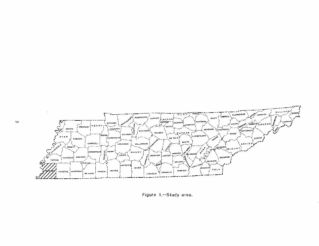
Figure 1 .--Study area .

water of the three principal streams entering the Mississippi Kiver in the vicinity of Memphis, severe localized flooding for short duration is a threat from the smaller streams. This flooding is caused by intense thunderstorms that are common in the early spring and summer.

APPROACH TO PROBLEM

A network of streamflow and rainfall gages was established to provide a data base. Consideration was given to having the gages distributed uniformly over the area with a wide range in drainage area size, basin slope, and impervious area. A representative range in the basin characteristics is needed for the results to have area1 application.

A continuous record of both rainfall and stage data was collected for 8 years at each gaging station. Discharge measurements were made during floods to define the stage-discharge relations. These reiations were used to convert stage data to discharge data. The rainfall data and discharge hydrograph during each storm runoff event were needed for modeling procedures. The rainfall data were assumed to represent the average rainfall distributed uniformly over the drainage basin. The discharge hydrograph was the response initiated by the rainfall and represented the temporal distribution of the runoff.

The reliability of flood-frequency data estimated from observed flood peaks is primarily dependent upon the length of observed record. For all stations used in this report, the length of record was too short to produce reliable flood-frequency estimates from the observed data. Thus to improve that reliability, observed records were used to derive synthetic flood- frequency data with a U.S. Geological Survey rainfall-runoff model developed by Dawdy and others (1972) in combination with a method developed by Lichty and Liscum (1978). The model is calibrated for each station using observed data from about 30 storms so that the simulated hydrographs fit the observed nydro- graphs as closely as possible. The calibrated model is then used to simulate flood peaks for long-term rainfall and evaporation data representative of the study area. Rainfall measured by the National Weather Service during 1898, 1900-18, and 1920-76 is assumed to represent the rain that fell at each gaging station. These 77 years of rainfall data at Memphis and pan-evaporation data from Mississippi State University were input for the model to simulate 77 annual peak discharges.

The simulated annual peak discharges were used in log-Pearson Type 111 analyses to estimate a flood-frequency curve for each station. Flood discharges for the 2-, 5-, lo-, 25-, 50-, and loo-year recurrence intervals -were analyzed by regression techniques to derive equations that relate flood discharge to physcial basin characteristics.

The model simulated discharge hydrographs for each of the storms that produced the 77 annual peak discharges. Storm runoff or flood volume was measured under each of the simulated hydrographs. The simulated storm runoff volumes were used in log-Pearson Type III analyses to estimate a storm runoff frequency curve for each station. Storm runoff volumes for the 2-, 5-, lo-, 25-, 50-, and loo-year recurrence interval were analyzed by regression techniques to derive equations that relate storm runoff to physical basin characteristics.

Discharge hydrographs for individual storms can be estimated by using the unit hydrograph, lag time, and rainfall excess. Unit hydrographs were computed using the Clark (1945) method with the results of the model calibration.

DATA COLLECTION

A network of 27 streamflow and 37 rainfall gages was established to provide a data base. locations of the streamflow and rainfall sites are shown in figure 2. All streamflow and rainfall gages were equipped with digital recorders. The rainfall gages recorded accumulated totals at 5minute intervals. The streamflow gages recorded the stage of the stream every 5 minutes. These stages were converted to discharge using a stage-discharge relation. The stage-discharge relation was defined by making measurements during floods and plotting discharge versus the stage of the measurement. Each station was equipped with a crest-stage gage which recorded the peak stage to verify the digital record. The gages were routinely serviced at about l-month intervals, and immediately after each flood.

The recorded annual peaks at each station are shown in Supplement A near the end of this report. The maximum rainfall intensities recorded at each station are shown in Supplement 13.

RAINFALL- RUNOFF MODEL

The rainfall-runoff model, developed by Dawdy and others (1972) and modi- fied by Carrigan (19731, simulates flood peaks for small drainage basins. The general structure of the model, as summarized in a report by Lichty and Liscum (19781, is given in the following paragraph:

It is a simplified, conceptual, bulk-parameter, mathematical model of the surface-runoff component of flood-hydrograph response to storm rainfall. The model deals with three components of the hydrologic cycle--antecedent soil moisture, storm infiltration, and surface-runoff routing. The first component simulates soil- moisture conditions of the storm period through the application of moisture-accounting techniques on a daily cycle. Estimates of daily rainfall, evaporation, and initial values of the moisture storage variables are elements used in this component. The second component involves an infiltration equation (Philip, 1954) and certain assumptions by which rainfall excess is determined on a 5minute accounting cycle from storm-period rainfall. Storm rainfall may be defined at 5-, lo-, 15-, 30-, and 60-minute intervals, but loss rates and rainfall excess amounts are computed at 5- minute intervals. The third component transforms the simulated time pattern of rainfall excess into a flood hydrograph by trans- lation and linear storage attenuation (Clark, 1945).

The model is divided into three phases of optimization--runoff volume, timing, and peak. In both the volume and peak phases, soil-moisture accounting parameters (EVC, RR, BMSM, DRN) and soil-infiltration parameters (PSP, KSAT, RGF) are optimized. In the timing phase, routing parameters (TC, KSW) are

5

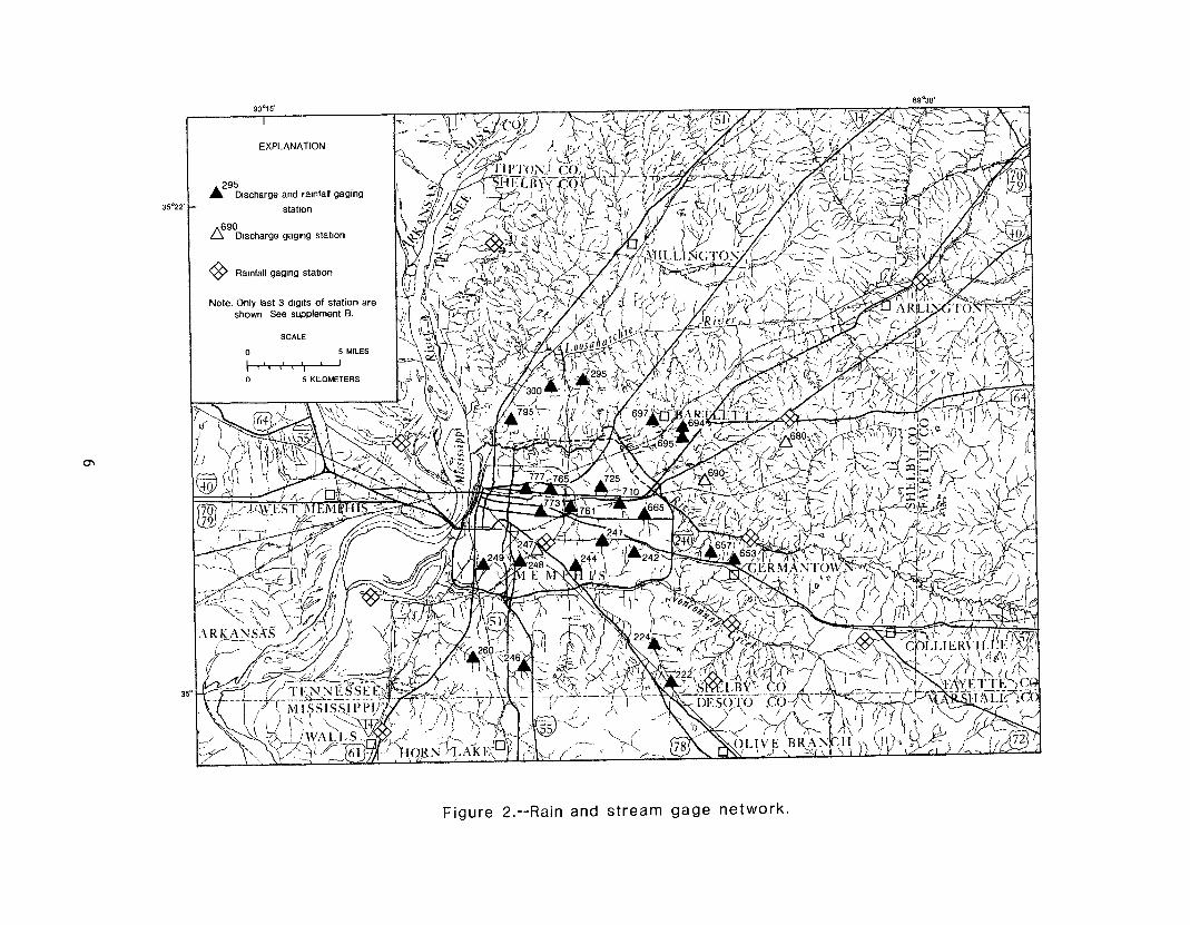
Figure 2.--Rain and stream gage network .

optimized. The model parameters and their definitions are summarized in table 1. For a more complete description of the model, see the report by Dawdy and others (1972).

Model Calibration

Data used to calibrate the model are daily rainfall and evaporation and concurrent unit rainfall and discharge. Unit data define individual storms and daily data define antecedent.moisture conditions. Unit discharge and rainfall data were collected at each gaged site. Evaporation data were collected at Mississippi State University. When missing record for rainfall and evaporation occurred, daily values were estimated to complete the record.

Runoff volume of a storm in urban areas is highly dependent on the impervious area. The impervious area which is determined for each basin and input into the model may not be effective impervious area. The effective impervious area would depend on the hydraulic connections between the impervious areas and the stream. The first phase of the model was to compute the standard error in volume for several different values of impervious area. The value of impervious area that yielded the lowest standard error in volume is the effective impervious area or optimized impervious area. This value of optimized impervious area was used as input into the model in lieu of the measured impervious area for the remainder at the calibration procedure.

During the model calibration of each basin, the 10 parameters listed in table 1 were optimized to produce closest fit of simulated peak discharge to observed peak discharge. About 30 storms were used for calibrating the model for each basin. The data were carefully screened and some storms were deleted from the calibraton primarily because of station equipment malfunction or lack of compatibility in the data. For example, it is implicit in the model that the rainfall measured at the rain gage represents the rainfall in the basin, but this can be erroneous, particularly for localized summer thundershowers. Consequently, some of the summer storms were not used because recorded discharge indicated that the recorded rainfail was not representative for the basin.

Four of the seven moisture accounting parameters were optimized to yield the lowest percentage of errors. These four parameters are BMSM, KSAT, PSP, and RGF. The values range from 1.04 to 10.3 from BMSM, 0.010 to 0.146 for KSAT, 0.380 to 5.980 for PSP, and 1.15 to 29.6 for RGF. The calibrated values are listed in table 2 for each station. In the calibration procedure, much interaction exists between parameters. Tne three antecedent moisture accounting parameters, RR, EVC, and DRN, were held at a constant value of 0.85, 0.75, and 1.0, respectively.

Runoff Simulation

The rainfall-runoff model can be calibrated with a short period of observed discharge record and used to simulate a long-period of annual peak discharge data. The model was used to simulate. 77 years of peak discharge

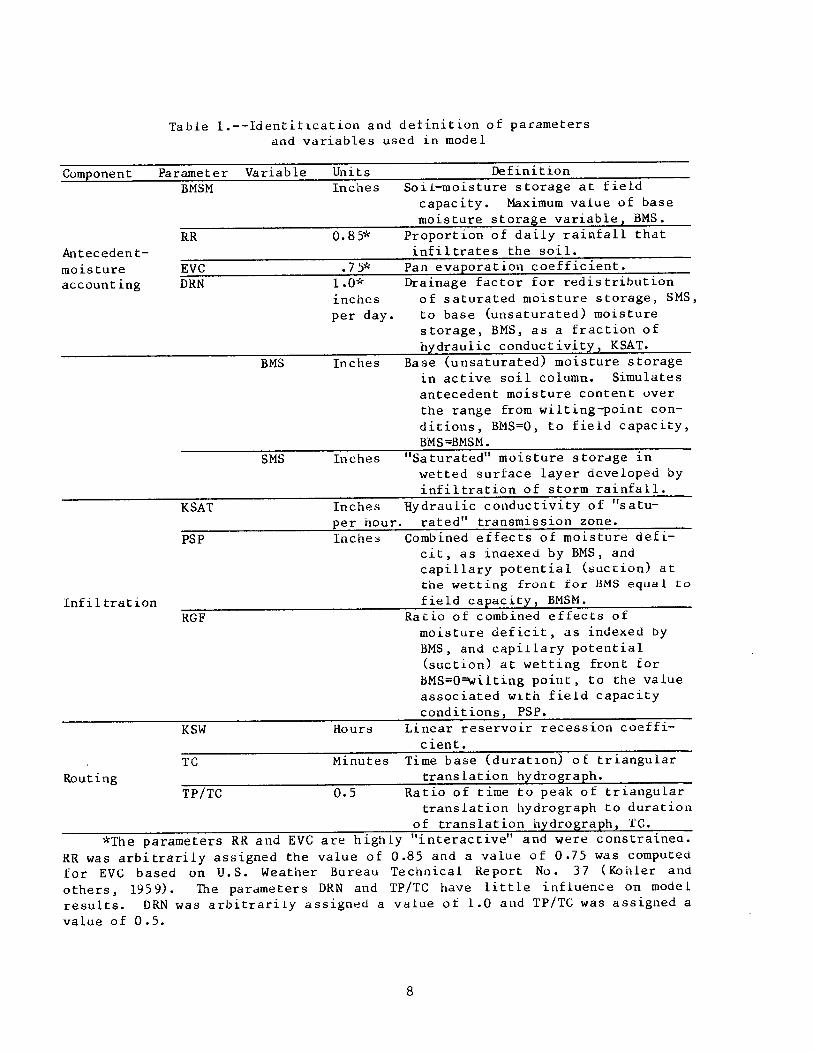
Table 1 .--Identification and definition of parametersand variables used in model

Table 2.--Calibrated model parameters

data. Inputs to the simulated program were daily rainfall and evaporation (to determine antecedent moisture conditions), unit rainfall, and the calibrated model parameters.

Five-minute rainfall data for approximately five storms per year for 77 years were obtained for the Memphis rain gage from the National Weather Ser- vice. One of these five storms is assumed to produce the annual peak discharge. The evaporation record was shorter than the rainfall record. Thus, part of the evaporation record was synthesized using existing data to produce a time frame common to the rainfall record. It was assumed that rainfall measured by the National Weather Service during the previous 77 years represents the rainfall at each gaging station. The rainfall data were used to drive the calibrated model to simulate annual peaks and volumes for each basin studied.

PEAK-DISCHARGE AND STORM RUNOFF FREQUENCY CURVES

Peak discharges and storm runoff volumes estimated by methods in this report are expressed as floods of selected recurrence interval. A 5year flood for example may be expected to be equaled or exceeded on the average of once in 5 years or, 20 times in 100 years. This does not mean floods occur at uniformly spaced intervals. In fact, a flood of this magnitude can be equaled or exceeded more than once in the same year, or can occur in consecutive years. Another way of expressing recurrence interval is in terms of probability. A 5year flood has the probability of 0.2 of being equaled or exceeded in any given year.

Peak discharge frequency curves were developed at each site by the Lichty and Liscum method (1978) and by a log-Pearson type III analysis using simulated peaks. Both methods gave flood magnitudes that were similar to each other.

The first method, the Lichty and Liscum map model procedure (1978), used parameters optimized in the rainfall runoff model calibration. The estimating procedure required computation of an infiltration factor (F), in inches per hour, and lag time (LT), in hours, to be used in the equations for synthetic flood magnitudes. The infiltration factor (F) is computed by the following equation:

F = KSAT [l.O + 0.5 PSP (0.15 RGF + 0.8511

and lag time (LT) by:

LT = KSW + 0.5 TC

where PSP, RGF, KSW, and TC are as previously defined in table 1.

Infiltration factors in a basin are related to the surface material. T'nat in Memphis area can vary from sand and gravel to silt, clay, and chalk. The impervious areas due to man's activities range from near zero to 74 percent.

Lag times computed by procedures of Lichty and Liscum (1978) were compared with lag times computed from observed data. Lag times were computed as time from the centroid of excess rainfall to the centroid of storm runoff. These comparisons showed no significant discrepancies.

10

Calibrated parameters and climatic factors were used to generate synthetic flood magnitudes for each of the 27 gaging stations. The procedures for estimating flood magnitudes for 2, 25, and 100 years are described by Lichty and Liscum (1978). Climatic factors of 212, 652, and 904 for the 2-, 25-, and lOO- year floods respectively were taken from table 4 in Lichty and Liscum (1978).

Lichty and Liscum (1978) indicated that the map-model procedure tends to underestimate the discharge for higher recurrence interval floods. Their adjustment for this apparent bias is made by the following equation,

"unbiased" qi = Bi qi

where Bi is the bias factors averaged from data for a six-state area covered in their report, and qi is the map-model estimate of flood magnitudes for recurrence interval i* The values for Bi are: B2 = 0.98, B25 = 1.19, and BlOO = 1.29. This bias effect, based on Lichty and Liscum (19781, lessens in a north to south direction. In Memphis the flood magnitude estimates were adjusted for bias.

The urban flood peaks, estimated by the Lichty and Liscum method (1978), for 2-, 25-, and loo-year recurrence interval were used to define log-Pearson type III statistical parameters, (skew, standard deviation, and mean>. These statistical parameters were used to estimate urban peaks for the 5-, lo-, and 50-year recurrence intervals as described by the U.S. Water Resources Council (1981).

The second method, a log-Pearson type III analysis, used the 77 simulated annual peak discharges. Annual peak discharges which depart from the trend of the other annual peaks are outliers (extreme events). Outliers can cause the mathematically fit curve through the annual peaks to be in error. Most of the stations used had at least one simulated annual peak that was a low outlier. Outliers of low annual discharge caused the skew to lower the upper end of the frequency curves and underestimate the higher order discharges. The curves that were used were drawn in by hand through the 77 plotted points (fig. 3).

Lichty and Liscum (1978) indicate that the map-model estimates are more accurate than the observed estimates beyond the lo-year recurrence interval. Therefore, the Lichty and Liscum map model method (1978) was used as the estimate of the discharge frequency at each site. The flood magnitudes for selected recurrence intervals for both methods are shown in table 3.

The standard deviation and average difference between the two methods for all the sites used are shown to the right for each recurrence interval. The average difference is based on differences of the simulated frequency curves from the Lichty-Liscum frequency curves. For instance, on the average at the 2year recurrence interval, the simulated frequency curve is -7 percent from the Lichty-Liscum frequency curve.

Recurrence Standard Average interval, deviation, difference, in years in percent in percent

2 * 17 -7 5 22 -22

10 25 -23 25 25 -24 50 21 -19

100 16 -12

11

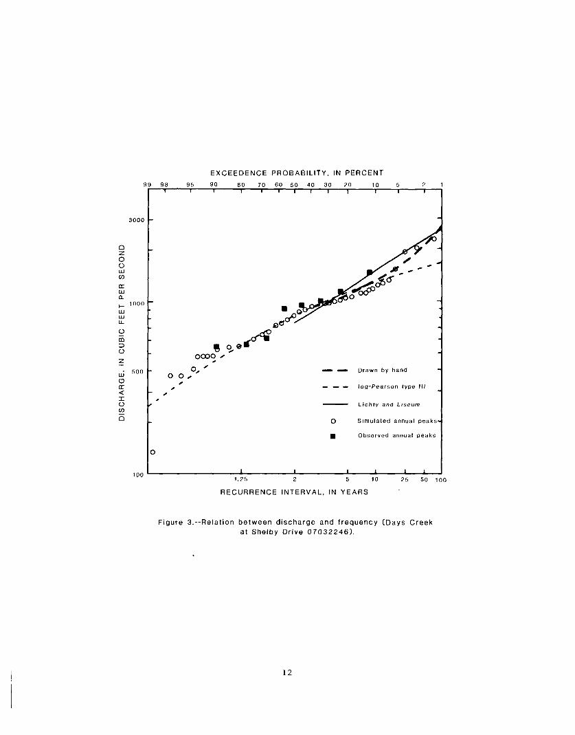
Figure 3.--Relation between discharge and frequency (Days Creekat Shelby Drive 07032246) .

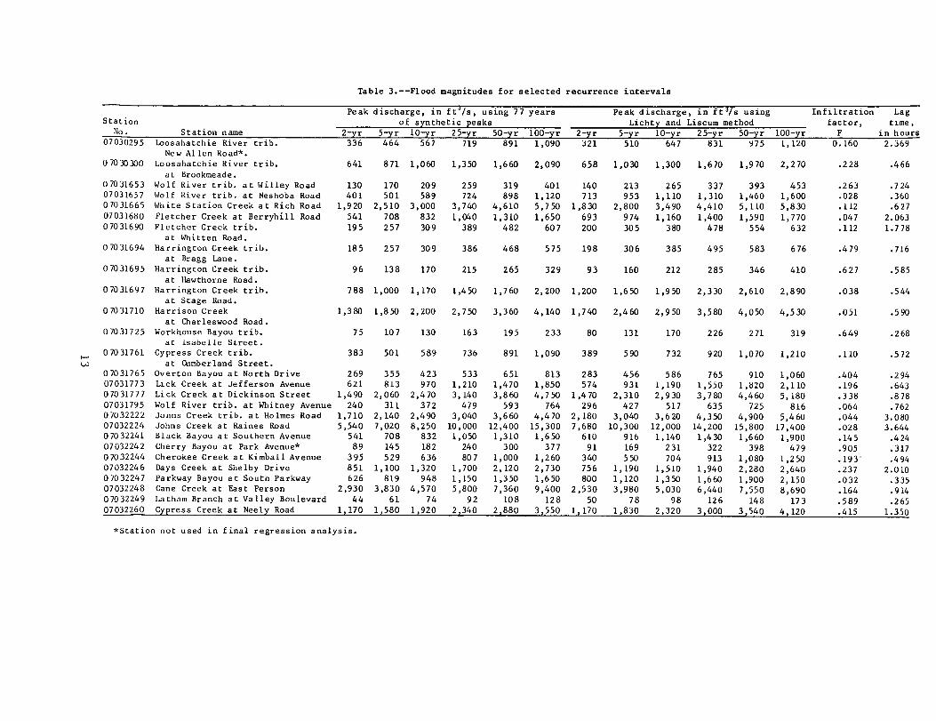
Table 3 .--Flood magnitudes for selected recurrence intervals

The storm runoff frequency curves were developed at each site by the log-Pearson type III analysis using the 77 years of simulated record. The runoff from the storm that produced the annual peak discharge was used in the analysis. Runoff for selected recurrence intervals are shown in table 4.

REGIONALIZATION OF PEAK DISCHARGE AND RUNOFF

Standard multiple linear regression techniques were used to relate basin characteristics to flood magnitudes and runoff volumes. Al 1 basin characteristics defined in this report were used in the regression analyses; however, only those that were statistically significant are included in the final equations.

Basin Characteristics

Nine basin characteristics were selected for use in the regression analyses. Some were selected because previous studies have shown them to be significant. Rainfall characteristics were not used in this study because approximately the same values are common to all sites. Table 5 gives the values of basin characteristics used. Definitions of the basin characteristics are as follows:

1. Drainage area, A. --The drainage area of the basin, in square miles.

2. Impervious area, I. --The percent of the basin that is covered by paved roads, paved parking lots, roofs, driveways, and sidewalks. If impervious area is less than 1 percent, use one. Impervious area was determined from aerial photographs and by field inspection.

3. Basin slope, BSL. --The average slope of the basin, in feet per mile, computed from U.S. Geological Survey topographic maps, using the for- mula described by Wisler and Brater (1959):

BSL = CL/A

where C = contour interval, in feet, L = total length of contours, in miles, and A = drainage area, in square miles.

4. Mean basin length, MBL. --The average flow length, in miles, between the gage site and the center of several equal-area subdivisions of the basin. The drainage basin was overlain with an appropriate sized grid to provide a minimum of 25 subdivisions.

5. Channel slope, S. --The channel slope, in feet per mile, computed between two points along the main channel --one point at 10 percent of the channel length, and the other point at 85 percent of the channel length. Both points are measured from the gaged site.

6. Main channel length, L.--The channel length, in miles, between the gaged site and the basin divide.

14

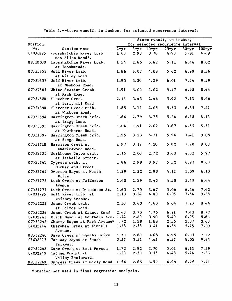
Table 4.--Storm runoff, in inches, for selected recurrence intervals

*Station not used in final regression analysis .

15

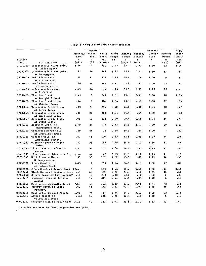
Table 5 .--Drainage-basin characteristics

7. Channel condition, P. --The average channel condition between points along the main channel at 100 percent, 75 percent, 50 percent, and 25 percent of the drainage area. If the channel is paved with concrete, use a value of 2; if unpaved, use a value of 1. The condition of the channel for partial paving can be estimated between 1 and 2.

8. Channel width, W. --The average channel width, in feet, at points along the main channel at 100 percent, 75 percent, 50 percent, and 25 per cent of the drainage area. At each point, widths representing various depths of flow were used to compute the average width.

9. Basin shape, SH. --The ratio of the channel length, L, to the average basin width, (A/L), or: SH = L2/A.

Regression Analyses

The maximum R2 technique of the stepwise procedure of SAS (1979) was used to derive the regression equations. tion. In this technique,

R is the coefficient of determina; variables that yield the greatest increase in R

are added first in deriving the regression equations. Log-transformations were made on all variables before the equations were derived. The first regression analysis included all basin characteristics for the 27 stations, however, only those that were statistically significant are included in the final equations.

Drainage areas used in the regression analyses ranged from 0.043 mi2 to 19.4 mi2, however, the distribution of size varied considerably within that range. The following summarizes the size distribution of drainage area for stations used.

Range in drainage area size (mi2)

0 - 0.1 0.1 - 0.25 0.25 - 0.50 0.50 - 1.50 1.50 - 4.00 4.00 - 10.00

10.00 - 20.00 Total stations

Number of stations

2 3 7 7 5 2 1

27

Values assigned to the channel condition ranges from following summarizes the distribution of channel condition used.

Number of Channel condition value stations

1.00 7 1.25 7 1.50 7 1.75 4 2.00 2

Total stations 27

1.00 to 2.00. The values for station

17

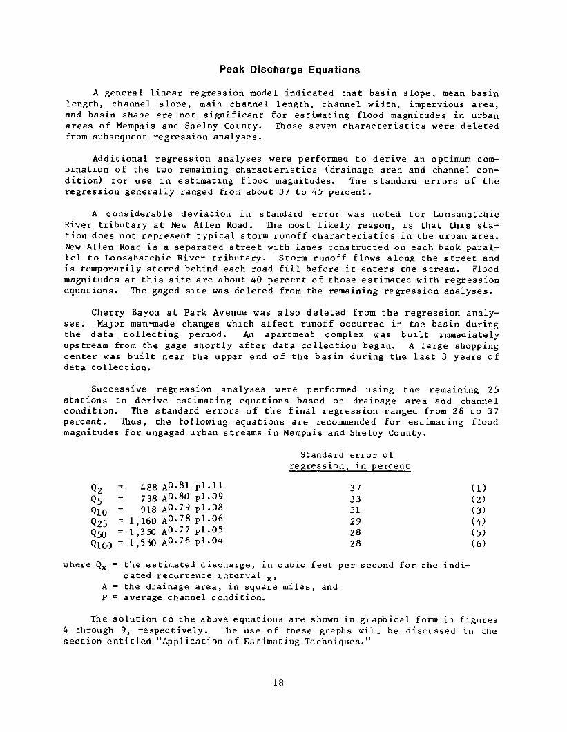
Peak Discharge Equations

A general linear regression model indicated that basin slope, mean basin length, channel slope, main channel length, channel width, impervious area, and basin shape are not significant for estimating flood magnitudes in urban areas of Memphis and Shelby County. Those seven characteristics were deleted from subsequent regression analyses.

Additional regression analyses were performed to derive an optimum combination of the two remaining characteristics (drainage area and channel condition) for use in estimating flood magnitudes. The standard errors of the regression generally ranged from about 37 to 45 percent.

A considerable deviation in standard error was noted for Loosahatchie River tributary at New Allen Road. The most likely reason, is that this station does not represent typical storm runoff characteristics in the urban area. New Allen Road is a separated street with lanes constructed on each bank paral- lel to Loosahatchie River tributary. Storm runoff flows along the street and is temporarily stored behind each road fill before it enters the stream. Flood magnitudes at this site are about 40 percent of those estimated with regression equations. The gaged site was deleted from the remaining regression analyses.

Cherry Bayou at Park Avenue was also deleted from the regression analyses. Major manlnade changes which affect runoff occurred in the basin during the data collecting period. An apartment complex was built immediately upstream from the gage shortly after data collection began. A large shopping center was built near the upper end of the basin during the last 3 years of data collection.

Successive regression analyses were performed using the remaining 25 stations to derive estimating equations based on drainage area and channel condition. The standard errors of the final regression ranged from 28 to 37 percent. Thus, the following equations are recommended for estimating flood magnitudes for ungaged urban streams in Memphis and Shelby County.

Standard error of regression, in percent

Q2 = 488 Ao.81 PI.11 37 (1) Q5 = 738 A0.80 pl.09 33 (2) Qlo = g18 &79 p1.08 31 (3) Q25 = 1,160 A0.78 p1.06 29 (4) Qso = 1,350 A0.77 P1.05 28 (5) Qloo = 1,550 ~0.76 ~1.04 28 (6)

where Qx = the estimated discharge, in cubic feet per second for the indicated recurrence interval x,

A = the drainage area, in square miles, and P= average channel condition.

The solution to the above equations are shown in graphical form in figures 4 through 9, respectively. The use of these graphs will be discussed in tne section entitled "Application of Estimating Techniques."

18

Figure 4.--Nomograph to determine relation of 2-year flood peak todrainage area and channel condition .

-

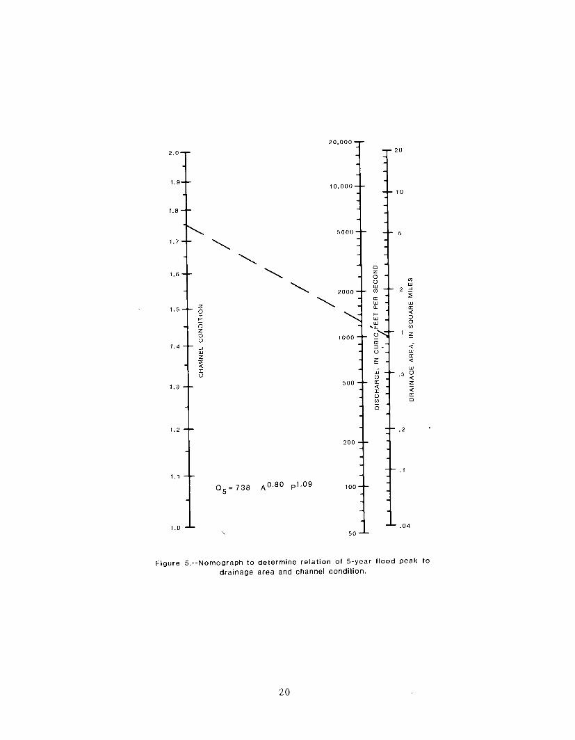
Figure 5 .--Nomograph to determine relation of 5-year flood peak to

drainage area and channel condition.

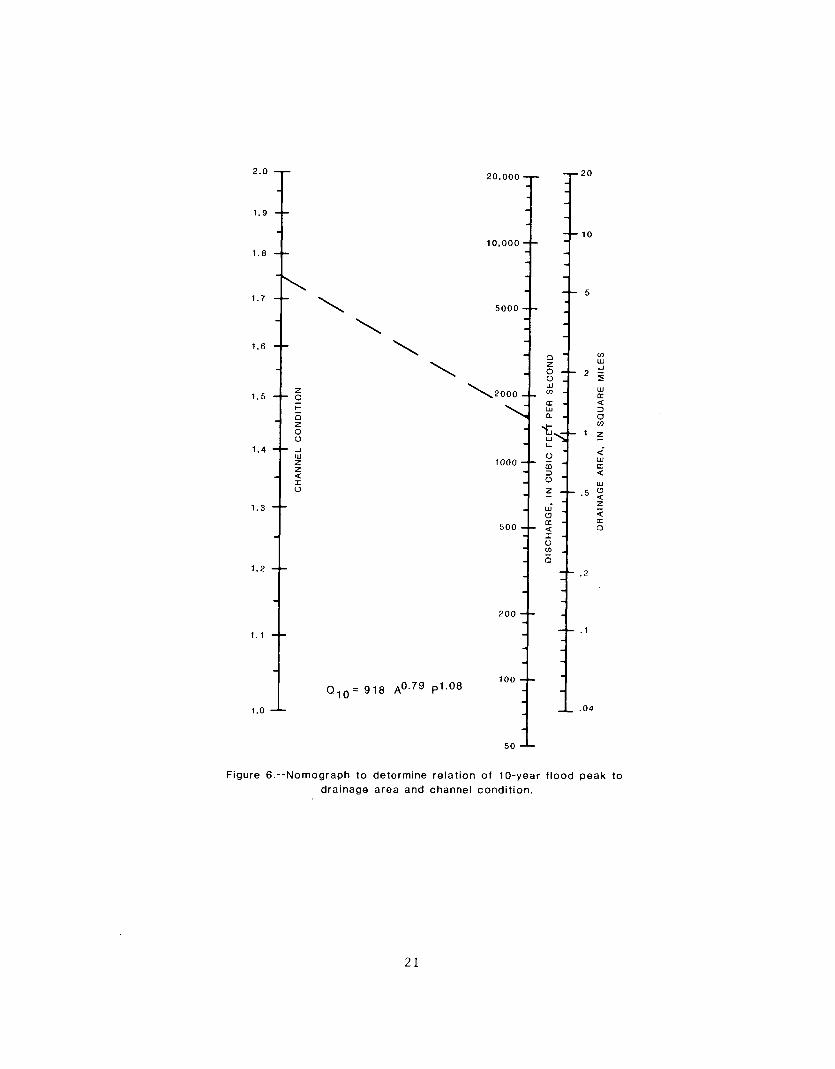
Figure 6.--Nomograph to determine relation of 10-year flood peak todrainage area and channel condition .

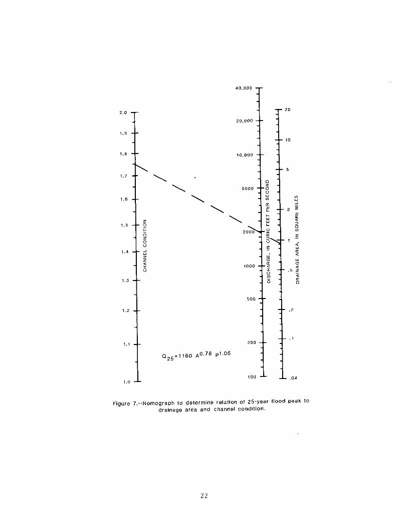
Figure 7.--Nomograph to determine relation of 25-year flood peak to

drainage area and channel condition .

Figure B .--Nomograph to determine relation of 50-year flood peak todrainage area and channel condition .

100

-4

Figure 9 .--Nomograph to determine relation of 100-year flood peak todrainage area and channel condition .

The accuracy of the equations for estimating flood magnitudes in this report was checked with graphical plots. 'Ibe graphs included plots of regression residuals versus drainage area, residuals versus channel conditions, and residuals versus magnitudes that were input into the regression analyses. The plotted points on each graph indicate that the parameters are not biased.

Storm Runoff Equations

The first regression analyses included all basin characteristics for the 27 stations. A general linear regression model indicated that drainage area is the only significant variable for estimating storm runoff. The following equations are recommended for estimating storm runoff, in inches, for ungaged urban streams in Memphis and Shelby County.

Standard error of regression, in percent

18 (7) 15 (8) 14 (9) 13 (10) 13 (11) 13 (12)

where Rx = storm runoff, in inches for the indicated recurrence interval x and

A = the drainage area, in square miles.

The solution to the above equations are shown in graphical form in figure 10. The use of this graph will be discussed in the section entitled "Applica- tion of Estimating Techniques."

ACCURACY OF REGRESSION ANALYSES

Accuracy of the regression analyses is computed from the difference between station data and the regression equation. The accuracy, in percent, referred to as standard error, is the range of error to be expected about two-thirds of the time. The errors associated with use of the equations to estimate flood magnitudes in ungaged streams are unknown. The errors are assumed to equal the standard errors of the regression equations.

A summary of the statistics of the regression analysis showing the order in which the characteristics were added to the regression equations, the standard error, and the final "F" values are shown for each recurrence interval in table 6. The "F" value aefines the significance of the independent variables. The larger the "F" value, the more significance the independent variable has in the equation.

The sensitivity of the regression equations for the 2-, 25-, and loo-year flood magnitudes to error in the drainage area (A) and channel condition (P) is shown below. All varrables are assumed to be constant except the one being

25

Figure 10 . --Relation of 2-, 5-, 10-, 25-, 50-, and 100-year storm runoff to drainage area .

Table 6.--Summary of statistics of the regression analysis

tested for sensitivity . That variable is assumed to contain an error rangingfrom +50 percent to -50 percent . For example, assume that drainage area, A,contains an error of +30 percent . Then the effect on computed 2-year peakdischarge would be +24 percent .

2 7

APPLICATION OF ESTIMATING TECHNIQUES

Methods for estimating flood discharges and storm runoff are given in equations 1 through 12 and graphically in figures 4 through 10. Basin characteristics needed to perform these calculations are drainage area and channel condition.

The following examples illustrate use of the equations and graphs to estimate the 25year flood and storm runoff.

Drainage area = 0.91 mi2 Channel conditions = 1.75

For the 25year flood, use equation 4.

Q25= 1,160 (0.91)"=78 (1.75?06 = 1,950 ft3/s

The 25-year flood can be determined graphically using figure 7. Enter the figure with channel condition (1.75) along the top line. Draw a straight line to drainage area (0.91) along the bottom line. The discharge can be read where this line intercepts the middle line. From this example, 25-year flood is estimated to be 1,950 ft3/s.

the magnitude of the

For the 25year storm runoff, use equation 10.

R25 = 5.26 (0.91)"*05 = 5.24

The 25-year storm runoff can also be determined graphically using figure 10. Enter figure 10 with drainage area (0.91) on the horizontal scale. Move vertically to the 25-year line. Move horizontally and read the storm runoff of about 5.24 inches from the vertical scale.

DISCHARGE HYDROGRAPHS

Occasionally the designer is interested in the peak discharge and runoff for a particular flood and a hydrograph showing the duration of the flood. This information is valuable when timing and storage must be considered in the design. Discharge hydrographs can be developed for individual floods by using the unit hydrograph method and- the appropriate rainfall excess. Methods of computing lag time, unit hydrographs, rainfall excess, and peak discharge are described in the following sections.

Lag Time

Lag time is defined as the time in hours from the center of mass of rainfall excess to the center of mass of the resulting runoff. The lag time for each station computed from parameters TC and KSW in the rainfall-runoff model calibration procedure is listed in table 3. The lag time for each basin is an average based on data collected for about 30 storms during a period of about 8 years.

28

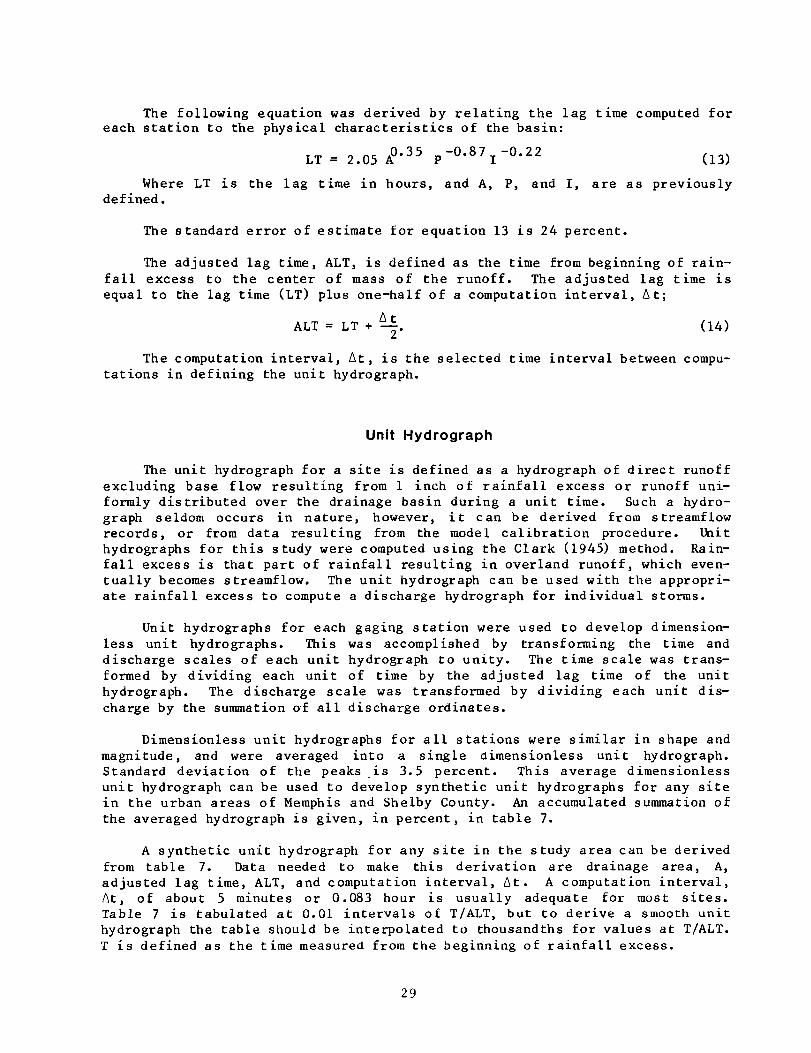
The following equation was derived by relating the lag time computed for each station to the physical characteristics of the basin:

LT _ 2 o5 8.35 P-0.87T-0.22 - . (13)

Where LT is the lag time in hours, and A, P, and I, are as previously defined.

The standard error of estimate for equation 13 is 24 percent.

The adjusted lag time, ALT, is defined as the time from beginning of rainfall excess to the center of mass of the runoff. The adjusted lag time is equal to the lag time (LT) plus one-half of a computation interval, At;

At ALT = LT + ?. (14)

The computation interval, At, is the selected time interval between compu- tations in defining the unit hydrograph.

Unit Hydrograph

The unit hydrograph for a site is defined as a hydrograph of direct runoff excluding base flow resulting from 1 inch of rainfall excess or runoff uniformly distributed over the drainage basin during a unit time. Such a hydrograph seldom occurs in nature, however, it can be derived from streamflow records, or from data resulting from the model calibration procedure. Unit hydrographs for this study were computed using the Clark (1945) method. Kain- fall excess is that part of rainfall resulting in overland runoff, which even- tually becomes streamflow. The unit hydrograph can be used with the appropriate rainfall excess to compute a discharge hydrograph for individual storms.

Unit hydrographs for each gaging station were used to develop dimensionless unit hydrographs. This was accomplished by transforming the time and discharge scales of each unit hydrograph to unity. The time scale was transformed by dividing each unit of time by the adjusted lag time of the unit hydrograph. The discharge scale was transformed by dividing each unit discharge by the summation of all discharge ordinates.

Dimensionless unit hydrographs for all stations were similar in shape and magnitude, and were averaged into a single dimensionless unit hydrograph. Standard deviation of the peaks ,is 3.5 percent. This average dimensionless unit hydrograph can be used to develop synthetic unit hydrographs for any site in the urban areas of Memphis and Shelby County. An accumulated summation of the averaged hydrograph is given, in percent, in table 7.

A synthetic unit hydrograph for any site in the study area can be derived from table 7. Data needed to make this derivation are drainage area, A, adjusted lag time, ALT, and computation interval, At. A computation interval, At, of about 5 minutes or 0.083 hour is usually adequate for most sites. Table 7 is tabulated at 0.01 intervals of T/ALT, but to derive a smooth unit hydrograph the table should be interpolated to thousandths for values at TIALT. T is defined as the time measured from the beginning of rainfall excess.

29

Table 7 .--Summation for synthetic unit hydrographs

The procedure for deriving a synthetic unit hydrograph from table 7 is asfollows :

1 . Select a computation interval, 4t .

2 . Compute adjusted lag time, ALT.

3. Compute T/ALT for increments of T equal to pt . The values of T/ALTshould be listed up to and including 3.00 .

4 . Tabulate the corresponding percentages from the summation table .These are accumulated distribution percentages for the desired unithydrograph at intervals equal to At .

30

5. Take differences between successive values of the accumulated percentages. This gives the distribution, in percent, of the unit hydrograph for the selected unit duration and time interval.

6. To convert the distribution percentage to a unit hydrograph, multiply each by 6.453 A/At. At must be in hours.

The unit hydrograph can be used with the rainfall excess to derive a discharge hydrograph.

Runoff

The method used in this study to convert rainfall to runoff is a computer model and cumbersome to use by manual methods. At least 2 months of antecedent rainfall and evaporation data are needed for input. Mathematical iterations to compute the results can be time consuming. To eliminate this laborious procedure, a simplified method for computing runoff is given below.

Rainfall excess or runoff, RE, was computed for each rise during model calibration for each station. A regression analysis was made relating total runoff to total rainfall using the rises on all the stations in this study. Antecedent moisture conditions which affect runoff were related to rainfall during the previous 3 days and to the month in which the rise occurred. Dummy variables for each month were used in the regression analysis to account for the seasonal effect on runoff. The following equation was derived relating runoff to rainfall:

RE = c RF1.18 Rl0.28 R20.15 R30.09 (15)

where RE = the rainfall excess or runoff, in inches; c = a regression constant for the month X;

RF = the storm rainfall, in inches; and Rl, R2, and R3 = the daily rainfall, in inches, plus 1.00, respectively, for

the first, second, and third day prior to the day for which runoff is computed.

The regression constant, C, is tabulated below for each month. The standard error of equation 15 is 27 percent. The standard errors in volume for each station using the computer model are shown in table 2. The average of these errors from table 2 is 24.8 percent. Therefore, the simplified method of computing runoff using equation 15 is almost as accurate as using the model.

Equation 15 was derived using total runoff and total rainfall. However, it can be used to compute unit runoff provided unit rainfall data is available. Rainfall data should be tabulated as accumulated totals for each time interval. Each accumulated total is used in equation 15 to compute an accumulated runoff. Unit runoff can then be determined by the differences in successive values of accumulated runoff.

31

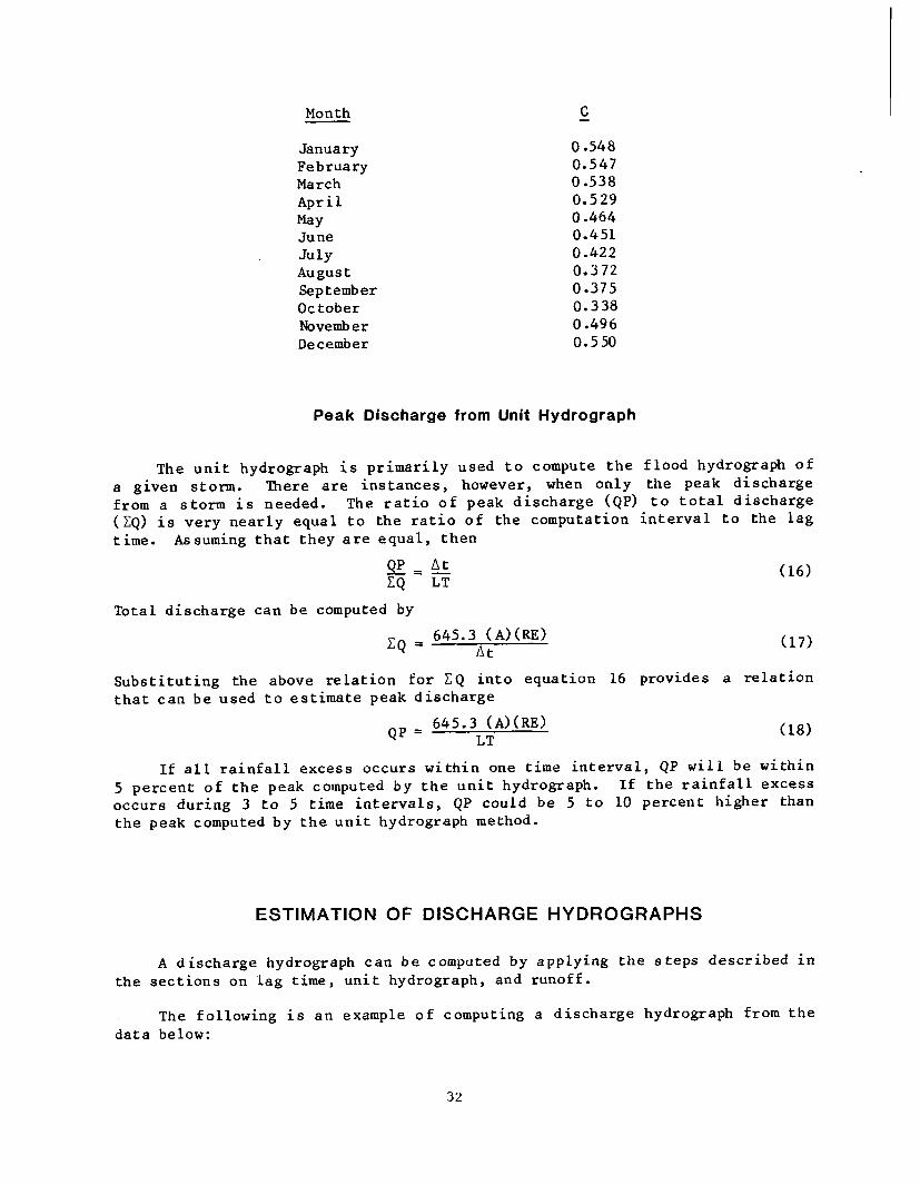
Month

January February March April %Y June July August September October November December

C

0.548 0.547 0.538 0.529 0.464 0.451 0.422 0.372 0.375 0.338 0.496 0.550

Peak Discharge from Unit Hydrograph

The unit hydrograph is primarily used to compute the flood hydrograph of a given storm. There are instances, however, when only the peak discharge from a storm is needed. The ratio of peak discharge (QP) to total discharge (CQ) is very nearly equal to the ratio of the computation interval to the lag time. Assuming that they are equal, then

QP At -=- CQ LT

Total discharge can be computed by

IQ = 645.3 (A)(RE) At

(16)

(17)

Substituting the above relation for CQ into equation 16 provides a relation that can be used to estimate peak discharge

QP = 645.3 (A)(RE) LT (18)

If all rainfall excess occurs within one time interval, QP will be within 5 percent of the peak computed by the unit hydrograph. If the rainfall excess occurs during 3 to 5 time intervals, QP could be 5 to 10 percent higher than the peak computed by the unit hydrograph method.

ESTIMATION OF DISCHARGE HYDROGRAPHS

A discharge hydrograph can be computed by applying the steps described in the sections on lag time, unit hydrograph, and runoff.

The following is an example of computing a discharge hydrograph from the data below:

32

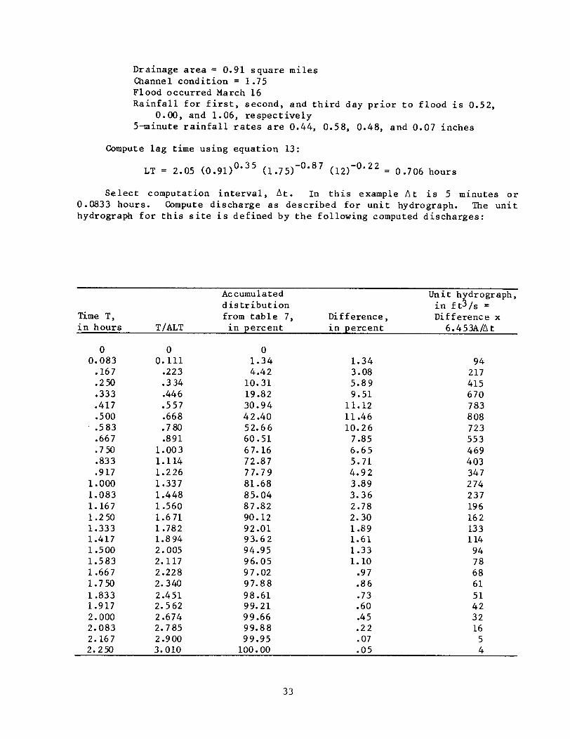
Drainage area = 0.91 square milesChannel condition = 1 .75Flood occurred March 16Rainfall for first, second, and third day prior to flood is 0.52,

0 .00, and 1 .06, respectively5-minute rainfall rates are 0.44, 0.58, 0.48, and 0.07 inches

Compute lag time using equation 13 :

LT = 2.05 (0 .91) 0 ' 35 (1 .75)-0'87 (12) -0 .22 = 0 .706 hours

Select computation interval, At . In this example At is 5 minutes or0 .0833 hours . Compute discharge as described for unit hydrograph . The unithydrograph for this site is defined by the following computed discharges :

33

Compute the rainfall excess as follows for this example, followingprocedures outlined in section on runoff .

Compute the discharge hydrograph as follows for this example . Transferpreviously computed discharges for unit hydrograph to column 2 . Transfer rain-fall excess to columns 3 through 6 . Multiply rainfall excess in first timeinterval by unit hydrograph and list in column 3 . Column 3 represents thedischarge hydrograph at the site caused by rainfall excess in the first timeinterval . Multiply rainfall excess in second time interval by unit hydrographand list in column 4 . Column 4 is lagged one time interval behind column 3 .Column 4 represents the discharge hydrograph at the site caused by the rainfallexcess in the second time interval . Repeat this procedure in columns 5 and 6,always lagging the previous column by one time interval . Sum columns 3 through6 laterally and record in column 7 . Column 7 is the discharge hydrograph atthe site .

SUMMARY

Simulated annual floods derived from a rainfall-runoff model were used todevelop flood-frequency relations for streams in urban areas in Memphis andShelby County, Tenn . The model was calibrated for 27 urban runoff sites withdrainage areas ranging from 0 .043 to 19 .4 square miles . Flood magnitudes forselected recurrence intervals were estimated by the map-model procedure devel-oped by Lichty and Liscum (1978) . Input data for that procedure include cli-matic factors and parameters calibrated in the rainfall-runoff model . Floodmagnitudes for selected recurrence intervals were also estimated using 77 yearsof simulated annual peak data . Both methods gave values that agreed reasonablywell . The Lichty and Liscum method was used in computing the final flood-frequency curves .

Standard regression techniques were used to derive equations for estimat-ing flood magnitudes for recurrence intervals of 2, 5, 10, 25, 50, and 100years for streams in urban areas of Memphis and Shelby County, Tenn. Drainagearea, impervious area, basin slope, mean basin length, channel slope, mainchannel length, channel condition, channel width, and basin shape were testedin the analyses, but only drainage area and channel condition were significant .Standard errors of regression ranged from 37 percent for the 2-year flood to28 percent for the 100year flood .

Standard regression techniques were used to derive equations for comput-ing storm runoff for selected recurrence intervals . The basin characteristicneeded to make this computation is drainage area .

A technique is presented for estimating discharge hydrographs for individ-ual floods . This technique includes methods of computing a unit hydrograph,lag time, and rainfall excess or runoff .

SELECTED REFERENCES

Boning, C. W., 1977, Preliminary evaluation of flood frequency relations in the urban areas of Memphis, Tennessee: U.S. Geoiogical Survey Water-Resources Investigations Report 77-132, 57 p.

Carrigan, P. H., Jr., 1973, Calibration of U.S. Geological Survey rainfall- runoff model for peak flow synthesis-natural basins: Reston, Virginia, U.S. Geological Survey open-file report, 109 p.

Carrigan, P. H., Dempster, G. R., and Bower, D. E., 1977, User's guide for U.S. Geological Survey rainfall-runoff model--revision of Open-File Report 74-33: U.S. Geological Survey Open-File Report 77-884, 273 p.

Clark, C. O., 1945, Storage and the unit hydrograph: American Society of Civil Engineers Transactions, v. 110, p. 1419-46.

Dawdy, D. R., Lichty, R. W., and Bergmann, J. M., 1972, A rainfall-runoff simulation model for estimation of flood peaks for small drainage basins: U.S. Geological Survey Professional Paper 506-B, 28 p.

Kohler, M. A., Nordenson, T. J., and Baker, D. R., 1959, Evaporation maps for the United States: Department of Commerce, U.S. Weather Bureau Technical Paper no. 37, 13 p., 5 pl.

Laenen, Antonius, 1980, Storm runoff as related to urbanization in the Port- land, Oregon-Vancouver, Washington area: U.S. Geological Survey Water- Resources Investigations Report 80-689, 62 p.

Lichty, R. W., and Liscum, F., 1978, A rainfall-runoff modeling procedure for improving estimates of T-year (annual) floods for small drainage basins: U.S. Geological Survey Water-Resources Investigations Report 78-7, 44 p.

Neely, B. L., 1976, Floods in Louisiana, magnitude and frequency (3rd ed.): Louisiana Department of Highways, 339 p.

Olin, D. A., and gingham, R. H., 1982, Synthesized flood frequency of urban streams in Alabama: U.S. Geological Survey Water-Resources Investigations Report 82-0683, 39 p.

Philip, J. R., 1954, An infiltration equation with physical significance: Soil Science Society of Anerica Proceedings, v. 77, p. 153-157.

Randolph, W. J., and Gamble, C. R., 1976, Techniques for estimating magnitude and frequency of floods in Tennessee: Tennessee Department of Transporta- tion, 52 p.

SAS Institute, Inc., 1979, SAS Users Guide, 1979 Edition: 494 p.

Sauer, V. B., 1970, Rainfall-runoff-hydrograph relations for Northern louisiana: Louisiana Department of Public Works, 33 p.

U.S. Water Resources Council, 1981, Guidelines for determining flood-flow frequency: U.S. Water Resources Council Bulletin 17B, 183 p.

Wisler, C. O., and Brater, E. F., 1959, Hydrology (2d ed.): New York, John Wiley, 408 p.

36

SUPPLEMENT A.--Location and annual peak data for gaging stations

LOOSAHATCHIE RIVER BASIN

07030295 Loosahatchie River tributary at New Allen Road at Memphis, TN

LOCATION .--lat 35 ° 14'17", long 89 °57'04", Shelby County, Hydrologic Unit08010209, on right bank at downstream end of bridge at the intersection ofNew Allen Road and Hawkins Mill Road in Memphis, 0 .82 mi east of IllinoisCentral Gulf Railroad, and 3 .4 mi east of U.S . Highway 51 .

07030300 Loosahatchie River tributary at St . Elmo Avenue at Memphis, TN

LOCATION .--Lat 35 ° 13'56", long 89 ° 58'51", Shelby County, 120 ft downstream fromculvert under St . Elmo Avenue, at Memphis .

Annual peak data

SUPPLEMENT A.--Location and annual peak data for gaging stations--Continued

WOLF RIVER BASIN

07031653 Wolf River tributary at Willey Road at Germantown, TN

-LOCATION.--Lat,35°05'54", �long-89°48'36"-, Shelby_County, 16 ft upstream _fromculvert on Willey Road and 700 ft west of Cordova Road at Germantown.

Annual peak data

07031657 Wolf River tributary at Neshoba Road at Germantown, TN

LOCATION .--Iat 35 °06'21", long 89 °49'54", Shelby County, 30 ft upstream fromculvert on Neshoba Road and 150 ft west of Brookside Drive at Germantown .

Annual peak data


WOLF RIVER BASIN--Continued

07031665 White Station Creek at Rich Road at Memphis, TN

LOCATION .--Lat 35°08'09", long 89°53'37", Shelby County, at downstream side ofbridge on Rich Road, 2,000 ft west of White Station Road at Memphis .

Annual peak data

07031680 Fletcher Creek near Cordova, TN

LOCATION .--Lat 35°11'21", long 89°45'42", Shelby County, Hydrologic Unit08010210, on right bank at upstream side of bridge at Berryhill Road, 1 .3mi south of U.S . Highway 64, and 2 .5 mi north of Cordova.

Annual peak data



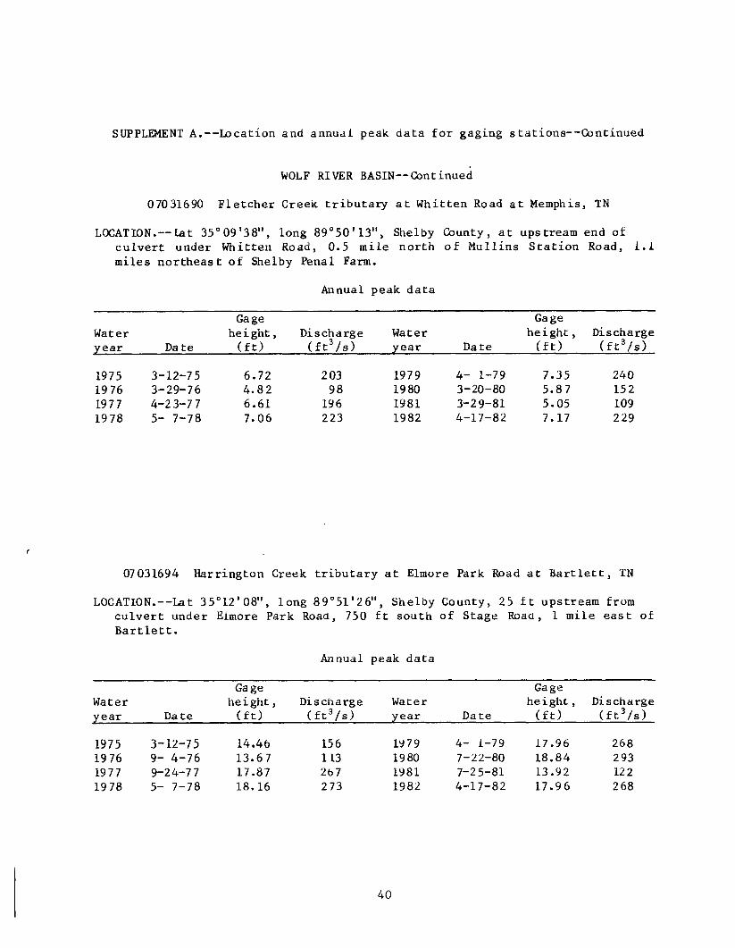
07031690 Fletcher Creek tributary at Whitten Road at Memphis, TN

LOCATION .--tat 35 ° 09'38", long 89 °50'13", Shelby County, at upstream end ofculvert under Whitten Road, 0.5 mile north of Mullins Station Road, 1.1miles northeast of Shelby Penal Farm .

Annual peak data

07031694 Harrington Creek tributary at Elmore Park Road at Bartlett, TN

LOCATION.--Iat 35 °12' 08", long 89 ° 51'26", Shelby County, 25 ft upstream fromculvert under Elmore Park Road, 750 ft south of Stage Road, 1 mile east ofBartlett .

Annual peak data

SUPPLEMENT A.--Location and annual peak data for gaging s tations--Continued

WOLF RIVER BASIN-- Continued

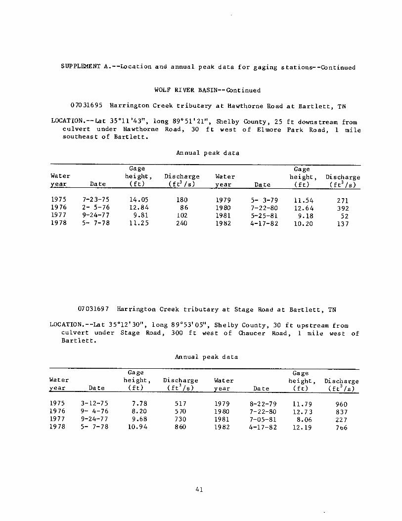
07031695 Harrington Creek tributary at Hawthorne Road at Bartlett, TN

LOCATION .--Lat 35 °11'43", long 89 ° 51'21", Shelby County, 25 ft downstream fromculvert under Hawthorne Road, 30 ft west of Elmore Park Road, 1 milesoutheast of Bartlett .

Annual peak data

07031697 Harrington Creek tributary at Stage Road at Bartlett, TN

LOCATION .--Lat 35°12'30", long 89 °53'05", Shelby County, 30 ft upstream fromculvert under Stage Road, 300 ft west of Chaucer Road, 1 mile west ofBartlett .

Annual peak data



07031710 Harrison Creek at Charleswood Road at Memphis, TN

LOCATION .--Lat 35 ° 08'34", long 89 ° 55'00", Shelby County, upstream side ofbridge at Charleswood Road, 300 ft west of Waring Road, at Memphis .

Annual peak data

07031725 Workhouse Bayou tributary at Isabelle Street at Memphis, TN

LOCATION .-- Lat 35°09'24", long 89°56'01", Shelby County, 200 ft upstream fromculvert under Isabelle Street, at Memphis .

Annual peak data



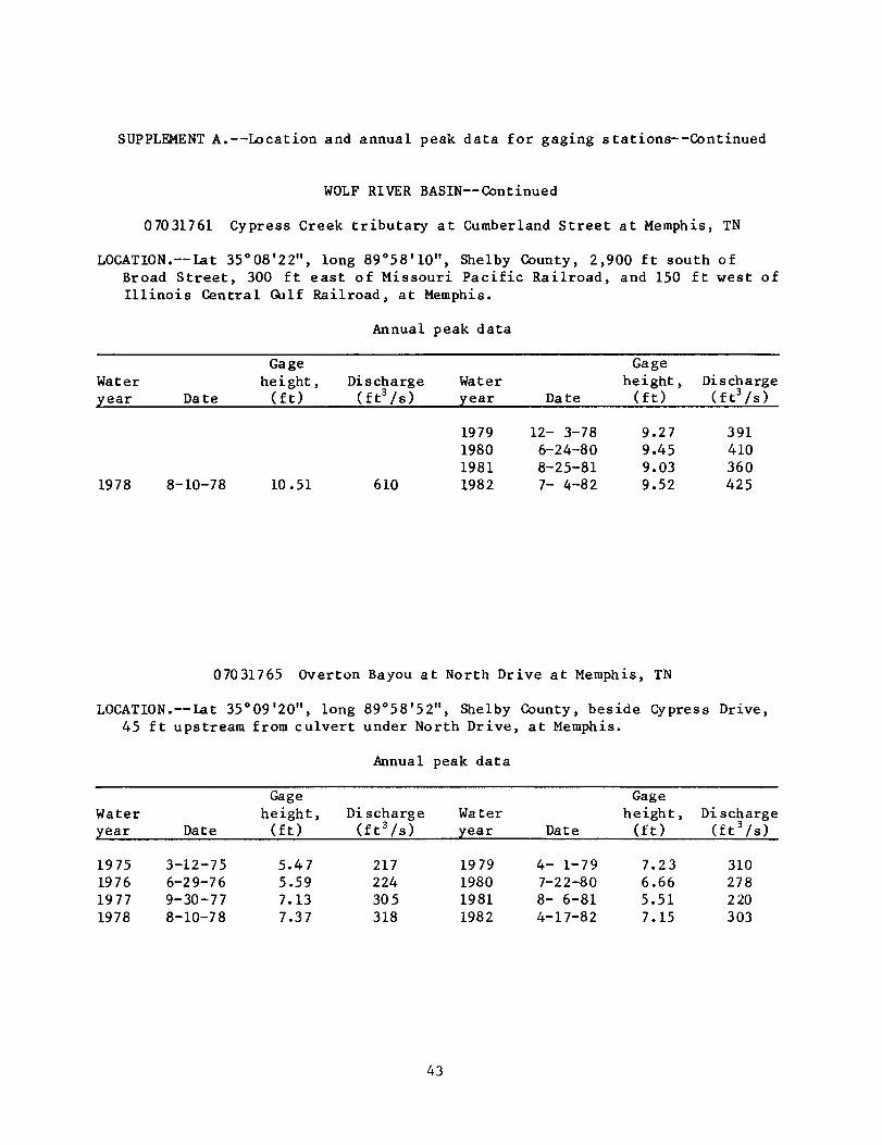
07031761 Cypress Creek tributary at Cumberland Street at Memphis, TN

LOCATION .--Lat 35°08'22", long 89°58'10", Shelby County, 2,900 ft south ofBroad Street, 300 ft east of Missouri Pacific Railroad, and 150 ft west ofIllinois Central Gulf Railroad, at Memphis .

Annual peak data

07031765 Overton Bayou at North Drive at Memphis, TN

LOCATION .--Lat 35 ° 09'20", long 89 °58'52", Shelby County, beside Cypress Drive,45 ft upstream from culvert under North Drive, at Memphis .

Annual peak data



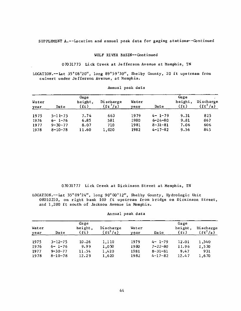
07031773 Lick Creek at Jefferson Avenue at Memphis, TN

LOCATION.--lat 35 ° 08'20", long 89 °59'30", Shelby County, 20 ft upstream fromculvert under Jefferson Avenue, at Memphis .

Annual peak data

07031777 Lick Creek at Dickinson Street at Memphis, TN

LOCATION .--Let 35°09'24", long 90°00'12", Shelby County, Hydrologic Unit08010210, on right bank 100 ft upstream from bridge on Dickinson Street,and 1,200 ft south of Jackson Avenue in Memphis .

Annual peak data

SUPPLEMENT A.--Location and annual peak data for gaging stations- -Continued


07031795 Wolf River tributary at Whitney Avenue at Memphis, TN

LOCATION .--Lat 35°12'31", long 90°01'15", Shelby County, at upstream end ofculvert under Whitney Avenue, at Memphis.

Annual peak data

NONCONNAH CREEK BASIN

07032222 Johns Creek tributary at Holmes Road near Memphis, TN

LOCATION.--Lat 35 °00'20", long 89 °52'16", Shelby County, Hydrologic Unit08010211, on left bank at upstream side of bridge at Holmes Road, 1,200 fteast of St . Louis-San Francisco Railroad, 2.0 mi east of U .S . Highway 78,and 2 .2 mi southeast of Memphis city limits .

Annual peak data


NONCONNAH CREEK BASIN--Continued

07032224 Johns Creek at Raines Road at Memphis, TN

` LOCATION .--lat'35°02'05", long 89°53'10", Shelby County, Hydrologic Unit08010211, on right bank at upstream side of Raines Road, 500 ft west ofMendenhall Road, and 1 .0 mi south of Winchester Road in Memphis .

Annual peak data

07032241 Black Bayou at Southern Avenue at Memphis, TN

LOCATION .--Lat 35°06'55", long 89 ° 56'00", Shelby County, Hydrologic Unit08010211, on right bank 130 ft downstream from Southern Avenue, and 150 fteast of Normal Street in Memphis .

Annual peak data



07032242

Cherry Bayou at Park Avenue at Memphis, TN

LOCATION ;--Lat 35 ° 06'24", long 89'54'13", Shelby County, 20 ft downstream fromculvert under Park Avenue, 150 ft west of Colonial Road, at Memphis .

Annual peak data

07032244

Cherokee Creek at Kimball Avenue at Memphis, TN

LOCATION .--Lat 35 ° 05'43", long 89 ° 57'31", Shelby County, at downstream end ofculvert under Kimball Avenue, at intersection of Alamo Street, at Memphis .

Annual peak data



07032246 Days Creek at Shelby Drive at Memphis, TN

LOCATION .--Lat 35°01'14", long 90°00'37", Shelby County, 75 ft upstream fromculvert under Shelby Drive, at Memphis .

Annual peak data

07032247 Parkway Bayou at South Parkway East at Memphis, TN

LOCATION .--Lat 35 ° 06'33", long 89 ° 59'41", Shelby County, between one-way lanesof South Parkway East, 100 ft west of Castalia Street, at Memphis .

Annual peak data



07032248 Cane Creek at East Person Avenue at Memphis, TN

LOCATION .--Lat 35 ° 06'02", long 90° 00'43", Shelby County, Hydrologic Unit08010211, on left bank 40 ft upstream from bridge on East Person Avenue,0 .4 mi east of Elvis Presley Boulevard, 0 .6 mi south of South Parkway Eastin Memphis, and at mile 2.8 .

Annual peak data

07032249 Latham Branch at Valley Boulevard at Memphis, TN

LOCATION .--Lat 35 ° 05'56", long 90° 02'43", Shelby County, between one-way lanesof Valley Boulevard, 200 ft downstream from Dison Avenue, at Memphis .

Annual peak data


MISSISSIPPI CREEK BASIN--Continued

07032260 Cypress Creek at Neely Road at Memphis, TN

LOCATION .--lat 35 °01'36", long 90° 03'23", Shelby County, Hydrologic Unit08010211, on right bank at downstream end of bridge on Neely Road, 1 .8 miwest of U.S . Highway 51 and 1 .1 mi southeast of U.S . Highway 61 in Memphis .

Annual peak data

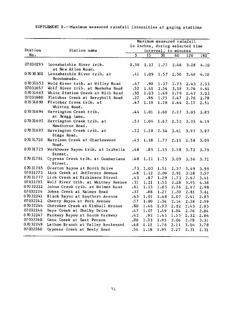
SUPPLEMENT B .-Maximum measured rainfall intensities at gaging stations

Documents

FLOOD FREQUENCY AND STORM RUNOFF OF URBAN … · flood frequency and storm runoff of urban areas of memphis and shelby county, tennessee ... iv . flood frequency