Embed Size (px)
Citation preview

1 C:\Documents and Settings\spallemoni\My Documents\gb\DOCS\flood_brown_SG_Final2009.doc
iGETT Cohort 2, June 2008
Learning Unit Student Guide Template
Flood_brown_SG_June2008
Name: Gail Brown Institution: Kirkwood Community College Email: [email protected] Phone: 319-398-5899 ext 4102 2008 Flood water analysis A comparison of Iowa June 2008 flood boundaries, one set drawn from Landsat Imagery using ENVI and NDWI, and one the flood boundaries drawn by Linn County GIS Department using imagery that was flown at the time of the flood.

2 C:\Documents and Settings\spallemoni\My Documents\gb\DOCS\flood_brown_SG_Final2009.doc
Part 1 – Overview of Topic
Problem In June 2008, Cedar Rapids, IA, experienced the worst flood on record. The water crested 12 feet above the flood boundaries of 1993. Linn County hired Pictrometry to take aerial photos at the time of the flood. County personnel digitized official flood boundaries from that imagery. USGS acquired the flood imagery from Landsat 5 on June16, 2008, one day after the water started to recede, for Linn County. By processing the Landsat imagery, and using ENVI to calculate a Normalized Difference Water Index, it will be possible to compare classified boundaries with hand digitized boundaries. This will make it possible to compare flood boundary accuracy using NDWI, and see what kind of data is lost or misclassified.
NOTE: The Landsat imagery is from June 16, 2008, by special arrangement with Landsat from disaster funding. This is the imagery available closest to the actual flood crest on June 14, 2008.
When the Cedar River crested, more than 3,900 homes were flooded and1,300 city blocks were inundated with water. Between 6,000 and 7,000 jobs were lost as hundreds of local businesses and local and county agencies were flooded. In this learning unit, students will use GIS to create base data including Cedar Rapids boundary, roads, and normal river boundaries. Landsat imagery from the June 16, 2008 – a day after the water began to recede - will be categorized as Wet or Not-Wet and overlaid on a base map. Finally, elevation contours will be made for the digital elevation models (DEMs) in an attempt to determine if the flood boundaries followed a specific contour.
Short Description The Cedar River travels through Linn County, IA, from NW to SE. It dissects the downtown area of Cedar Rapids, IA. Part of the city is within the 500-year floodplain, meaning there is a 0.2% chance of flooding per year; historically, Cedar Rapids flood levels have stayed within 19 feet. This learning unit will help students understand how GIS can be used to analyze flood situations. Using ENVI 4.5, students will have an opportunity to look at Landsat imagery and determine flood areas. A comparison of the digitized flood boundaries and Landsat flood boundaries will help students discern the strength/weaknesses of both, and give students a better understanding of the importance of resolution in decision-making processes. In this unit, students will work with ArcGIS and ENVI 4.5 in order to document the flood waters of the 2008 flood. Students will manipulate Landsat imagery using ENVI to classify pixels as water or not water. Using ArcGIS, this layer will be used as backdrop for the flood boundaries digitized by the city of Cedar Rapids using aerial imagery flown at the time of the flood. Differences in boundaries using the 0.5m aerial from the city of Cedar Rapids, as well

3 C:\Documents and Settings\spallemoni\My Documents\gb\DOCS\flood_brown_SG_Final2009.doc
as the city the street files, students will be able to delineate areas for which Landsat Imagery was wrongly classified.
Introduction Prior to working with Landsat images, it helps to have an idea of what comprises a cell and what that signifies. What follows is an outline of raster information. 1. Introduction to raster
1.1. Cells 1.1.1. fundamental unit of analysis in raster systems 1.1.2. represents a location 1.1.3. condition of a given cell is recorded as a numeric value for each cell
1.1.3.1. cell values related to earth property 1.1.4. Cell size
1.1.4.1. Area may be in meters/feet 1.1.4.1.1. Each side is equal 1.1.4.1.2. Can calculate area per cell 1.1.4.1.3. Can then calculate area per raster
1.1.5. a GRID is a regular arrangement of cells. 1.2. Layers
1.2.1. containers for handling regular arrays of cells 1.2.2. geographically referenced
1.2.2.1. can be stacked up, creating relationships
ACTIVITY-1: Raster Data Bring in the aerial photo of the Cedar Rapids area. Right click and go to properties. Answer the following questions regarding the imagery. What is the spatial reference
What is the cell size
What is the linear unit
WHAT IS SATELLITE IMAGERY? Watch the NASA video http://Landsat.gsfc.nasa.gov/

4 C:\Documents and Settings\spallemoni\My Documents\gb\DOCS\flood_brown_SG_Final2009.doc
Download Landsat Imagery Access the website: http://glovis.usgs.gov/
Click on Iowa on the map. This will open a new window. To download LandSat data, you need to know what path and row your area of interest falls into. You can click on the map to zoom to your area, or use the arrows on the screen to move scene by scene.
Make note of the path and row since you will be using this again. Path Row

5 C:\Documents and Settings\spallemoni\My Documents\gb\DOCS\flood_brown_SG_Final2009.doc
To download the data select ETM+ (1993-2003)
When you have the image you are interested in 1) Highlight the correct file in the Scene List
a) Click Add to bring the file name down to show in the lower window.
2) Click the download button in the bottom bar.
NOTE: If the data is labeled Downloadable, it is immediately available. Data that is no so labeled, can be ordered for free, though it may take several days to arrive.

6 C:\Documents and Settings\spallemoni\My Documents\gb\DOCS\flood_brown_SG_Final2009.doc
3) MetaData a) At any point, right click on the image you are interested and select metadata to learn
more about your data. The following screen will open.
The table to the left shows you the file size, the data the image was taken and cloud cover. It also has information regarding the extent of area covered.
ELP025R031_7T19991006 Naming convention on right http://landsat.usgs.gov/tools
LXSPPPRRRYYYYDDDGSIVV L = Landsat X = Sensor S = Satellite PPP = WRS Path RRR = WRS Row (Start and End Rows for multi-scenes) YYYY = Year DDD = Julian Day of Year1 GSI = Ground Station Identifier VV = Version
Landsat 7 ETM+ The Landsat 7 Enhanced Thematic Mapper Plus (ETM+) sensor includes a 15-meter (m) panchromatic band (band 8), as well as improved resolution (60 m) for the thermal infrared band (band 6). All bands have two gain settings (high and low) for increased radiometric sensitivity and dynamic range, with band 6 acquired in both high and low gain for all scenes.
For our final exercise, you will need information from the metadata, so prior to downloading the image when you locate the area you are looking for, fill in the following table.
1 Look up Julian Year on the internet and see what your Julian birthday is.

7 C:\Documents and Settings\spallemoni\My Documents\gb\DOCS\flood_brown_SG_Final2009.doc
Date Attribute Value
ID Acquisition Date Cloud Cover WRS 2 Path WRS 2 Row Zone Upper Left Corner Upper Right corner Lower Left Corner Lower Right Corner Scene Center Sun Azimuth Sun Elevation
ACTIVITY - 2:
Study the value assigned to each of the cells and compare that to what is in the field.
1) Measure cell value outside, 30m by 30m a) Note what is within the cell b) What does this have to do with cell classification? c) How much data is lost? d) What might the consequences be for the user?

8 C:\Documents and Settings\spallemoni\My Documents\gb\DOCS\flood_brown_SG_Final2009.doc
What is ENVI?
“ENVI is the premier software solution for processing and analyzing geospatial imagery used by GIS professionals, scientists, researchers, and image analysts around the world. ENVI software combines the latest spectral image processing and image analysis technology with an intuitive, user-friendly interface to help you get meaningful information from imagery.”2 This means, we can look at the individual cells to analyze the imagery. We will be using ENVI 4.5 to separate wet areas from dry areas to determine the flood boundaries. For this part of the exercise we will be using Landsat imagery from June 17, 2008. This image is courtesy USGS, and was paid for with USGS Disaster money. It was taken two days after the flood crested. Important Notes: EVNI opens several windows when working. In the directions below they are referred to as follows.
EVNI Window
Display Window
Scroll Window Zoom Window
Available Bands
Open ENVI Set Default Directories Before beginning work, it is helpful to set the file defaults to ensure that all files are saved in the appropriate location. Create a project folder on the C:\ Within that folder create the following folders:
Data Work folder Reflectance Radiance Images
1) On the ENVI window
a) Files
2 Introducing ENVI 4.5 (ITT)

9 C:\Documents and Settings\spallemoni\My Documents\gb\DOCS\flood_brown_SG_Final2009.doc
b) Preferences i) Default Directories tab
(1) Set the Data Directory to where the data is located (2) The Temp Directory by default will go to the system temp (3) Output Directory set to your workfolder
Add the Landsat imagery from June 17, 2008. 1) Files
a) Open external files b) Landsat c) Geotiff
2) In Enter TIFF/GEOTIFF Filenames windows navigate to a) C:\FloodProject\Data\Iowa Flood\Path25_Row31_June17_2008 b) Select all bands but Band 6
3) Available Bands window will open

10 C:\Documents and Settings\spallemoni\My Documents\gb\DOCS\flood_brown_SG_Final2009.doc
EXPLORE -1 4) Select band 7
1. Click load band 1. Display, scroll and zoom windows appear
2. Move red box in scroll window to look at full resolution data in the display window 1. What do you think is valuable about this map? 2. What do you think could make this map more useful?
Figure 1 The above image is centered on the area around Mays Island. Note the three bridges that were underwater at the time of the flood.
EXPLORE - 2 5) In Available Bands list GUI select RGB button
a) Select bands 3, 2 1

11 C:\Documents and Settings\spallemoni\My Documents\gb\DOCS\flood_brown_SG_Final2009.doc
b) Display 3,2,1 composite image i) Click Display #1 ii) Add new iii) Click Display #2 iv) Click to load RGB
6) What can you interpret visually from this image? 7) Repeat for band sets [4, 3, 2] [7,4, 2] [4, 5, 3]
EXPLORE - 3 8) Look at header information
a) Click on plus sign in front of Map Info Icon
b) What information do you see here? What does it tell you about the band? c) Do the same for two other bands d) What do you notice? Is the information the same or different?
EXPLORE - 4 1. In Display GUI select Enhance Image
1. Linear 2. Repeat using other stretches

12 C:\Documents and Settings\spallemoni\My Documents\gb\DOCS\flood_brown_SG_Final2009.doc
1. Linear 0-255 2. Gaussian 3. Equalization 4. Square root
Link Displays By linking displays, we are able to move simultaneously on two or more displays. This makes it possible to zoom in and out of the same area with ease.
1. Display a 3, 2, 1 image in Display #1 2. Display a 4, 5, 3 image in Display #2 3. In the Display GUI select tools
1. Link 2. Link displays
1. In Link GUI make sure Display #1 and Display #2 say yes
2. Click okay 4. In the Scroll window, move the red box around
1. Click in the display GUI to see a dynamic move
EXPLORE - 5 Pixel Values
1. In the display GUI select tools 1. Cursor location value 2. Move your cursor around the Display GUI and watch the values change in the
Cursors Location GUI Pixel Location
1. In the display GUI select tools 1. Pixel locater
2. Use the arrow button to toggle between UTM and geographic coord.
3. Use the lower arrows to move pixel by pixel To SAVE: File
1. Save Session to Script NOTE: To open the project later, go to file > execute script and locate the file saved.

13 C:\Documents and Settings\spallemoni\My Documents\gb\DOCS\flood_brown_SG_Final2009.doc
Stack
Stack is like grouping in ArcMap; it allows the manipulation and comparison of layers. This allows you to load all layers on one satellite imagine into the display window at once. 1) ENVI 4.5 Menus
a) Basic tools b) Layer stacking c) Import
i) Select from layers on your available bands list ii) Load 1-5 and Band 7 from the Iowa flood Folder iii) Ok
iv) Ok

14 C:\Documents and Settings\spallemoni\My Documents\gb\DOCS\flood_brown_SG_Final2009.doc
v) Set the file output name. Make sure this is a name that contains identifying information such as S7061708P25B31. This tells me it is a stack of Landsat 7 from 06.17.2008 of Path 32 Band 31. vi) Ok
Rename so we know which band is which.
1) ENVI Menu
a) File b) Edit ENVI Header

15 C:\Documents and Settings\spallemoni\My Documents\gb\DOCS\flood_brown_SG_Final2009.doc
c) Select the Layers one at a time d) Band 1 Blue e) Band 2 Green f) Band 3 Red g) Band 4 NIR h) Band 5 SWIR i) Band 7 SWIR1 (Click off of this band
before clicking ok) j) Ok k) Ok
Activity - 3 What do those band names mean? Landsat imagery has over 30-years of history. To truly value the significance of this data, and the potential use, it is important to understand more fully the data represented by the various bands. Using the USGS site, complete the following tables.
What Is Landsat? 1. Go to eros.usgs.gov/products/satellite/landsat7.html Read to answer these questions:
2. Describe the 8 bands that are provided. (fill in this table from your notes or find information at http://landsat.gsfc.nasa.gov/education/compositor/) When you find the colored bands on the Web page, look at the previous page where there is a chart.
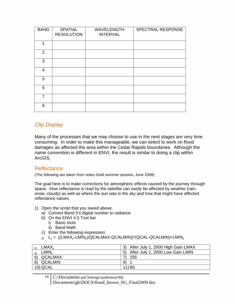
16 C:\Documents and Settings\spallemoni\My Documents\gb\DOCS\flood_brown_SG_Final2009.doc
BAND SPATIAL
RESOLUTION WAVELENGTH
INTERVAL SPECTRAL RESPONSE
1
2
3
4
5
6
7
8
Clip Display Many of the processes that we may choose to use in the next stages are very time consuming. In order to make this manageable, we can select to work on flood damages as affected the area within the Cedar Rapids boundaries. Although the name convention is different in ENVI, the result is similar to doing a clip within ArcGIS.
Reflectance (The following are taken from notes iGett summer session, June 2008) The goal here is to make corrections for atmospheric effects caused by the journey through space. How reflectance is read by the satellite can easily be affected by weather (rain, snow, cloudy) as well as where the sun was in the sky and how that might have affected reflectance values. 1) Open the script that you saved above.
a) Convert Band 5’s digital number to radiance b) On the ENVI 4.5 Tool bar
i) Basic tools ii) Band Math
c) Enter the following expression: d) Ly = ((LMAXy-LMINy)/QCALMAX-QCALMIN))*(QCAL-QCALMIN)+LMINy
2) LMAXy 3) After July 1, 2000 High Gain LMAX 4) LMINy 5) After July 1, 2000 Low Gain LMIN 6) QCALMAX 7) 255 8) QCALMIN 9) 1 10) QCAL 11) B5
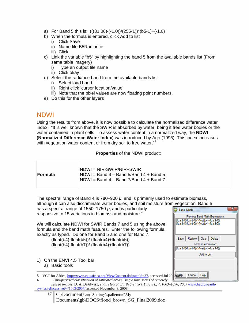
17 C:\Documents and Settings\spallemoni\My Documents\gb\DOCS\flood_brown_SG_Final2009.doc
a) For Band 5 this is: (((31.06)-(-1.0))/(255-1))*(b5-1)+(-1.0) b) When the formula is entered, click Add to list
i) Click Save ii) Name file B5Radiance iii) Click
c) Link the variable “b5” by highlighting the band 5 from the available bands list (From same table imagery) i) Type an output file name ii) Click okay
d) Select the radiance band from the available bands list i) Select load band ii) Right click ‘cursor location/value’ iii) Note that the pixel values are now floating point numbers.
e) Do this for the other layers
NDWI Using the results from above, it is now possible to calculate the normalized difference water index. “It is well known that the SWIR is absorbed by water, being it free water bodies or the water contained in plant cells. To assess water content in a normalized way, the NDWI (Normalized Difference Water Index) was introduced by Ago (1996). This index increases with vegetation water content or from dry soil to free water.”3
Properties of the NDWI product:
Formula
NDWI = NIR-SWIR/NIR+SWIR NDWI = Band 4 – Band 5/Band 4 + Band 5 NDWI = Band 4 – Band 7/Band 4 + Band 7
The spectral range of Band 4 is 780–900 μ, and is primarily used to estimate biomass, although it can also discriminate water bodies, and soil moisture from vegetation. Band 5 has a spectral range of 1550–1750 μ, and is particularly responsive to 15 variations in biomass and moisture.4 We will calculate NDWI for SWIR Bands 7 and 5 using the above formula and the band math features. Enter the following formula exactly as typed. Do one for Band 5 and one for Band 7.
(float(b4)-float(b5))/ (float(b4)+float(b5)) (float(b4)-float(b7))/ (float(b4)+float(b7))
1) On the ENVI 4.5 Tool bar
a) Basic tools 3 VGT for Africa, http://www.vgt4africa.org/ViewContent.do?pageId=27, accessed Jul 29, 2008. 4 Unsupervised classification of saturated areas using a time series of remotely sensed images, D. A. DeAlwis1, et al, Hydrol. Earth Syst. Sci. Discuss., 4, 1663–1696, 2007 www.hydrol-earth-syst-sci-discuss.net/4/1663/2007/ accessed November 3, 2008.

18 C:\Documents and Settings\spallemoni\My Documents\gb\DOCS\flood_brown_SG_Final2009.doc
b) Band Math i) Enter the above formula exactly as written ii) Click add to list
(1) If there is an error in your formula, you will receive an error message and will not be able to go on.
iii) Save iv) OK
c) Apply the formula i) With B4 highlighted in the Variables list ii) Select Band 4 in the Available list iii) Highlight Bd 5 (or B7) in the Variables list iv) Select Band 5 (or Band 7) in the Available list v) Save each to your workfolder vi) NDWIB5 or NDWIB7
2) Create a stack using Bands 1-5, 7 and the 2 NDWI images a) Name is StackNDWI57
Overlay Vector File 1) In display window select Overlay
a) Vectors i) Vector Parameters Window
(1) File (2) Open (3) C:\Flood Project LU\Data\CR_Data
(a) Change filter to Shapefile (4) Select CR_Bnds.shp (5) Verify projection at bottom is UTM
Zone 15 (6) OK
2) A Vector Parameter Window opens a) File b) Export Active Layer to ROI
i) Convert all records ii) OK
Figure 2: Result of Overlay; not the boundary outline on the map.

19 C:\Documents and Settings\spallemoni\My Documents\gb\DOCS\flood_brown_SG_Final2009.doc
3) In Display Menu
a) Overlay b) Region of Interest c) ROI Tool appears
i) File ii) Subset data via ROI iii) Select your data stack iv) In new window select ROI file v) Setout name to CR_Bnds vi) OK
d) New band will appear in Available Bands list
Classification
ACTIVITY – 4 Color by Number
The following handout contains an image with a grid overlaid. Using colored pencils, make each grid only one color and note what the color represents in a legend. Determine the color to use by what you see as the predominant characteristic of the grid, i.e., trees, water, grass, etc. Does the image represent the actual content of the cell? Classification adds color to individual cells in a similar fashion. Once the pixels numbers are ready to use, we can classify them to determine wet not-wet.
Unsupervised Classification
1) Classification
a) Unsupervised classification i) On the ENVI 4.5 tool bar select ii) Classification iii) Unsupervised iv) IsoData v) Select the StackNDWI57 vi) Set MAX number classes to 40 vii) Output Name UnsupStackNDWI57
b) When done, load the classified raster into a new display.
From ENVI Tutorial: “Clump and Sieve are used to generalize classification images. Sieve is usually run first to remove the isolated pixels based on a size (number of pixels) threshold, then clump is run to add spatial coherency to existing classes by combining adjacent similar classified areas.” Clump and Sieve provide means for generalizing classification images. Sieve is usually run first to remove the isolated pixels based on a size (number of pixels) threshold, and then clump is run to add spatial coherency to existing classes by combining adjacent similar classified areas

20 C:\Documents and Settings\spallemoni\My Documents\gb\DOCS\flood_brown_SG_Final2009.doc
Sieve
1) ENVI 4.5 Tool bar a) Classification b) Post classification c) Sieve classes
i) In the Sieve Parameters Window, select UnsupStackNDWI57 ii) Keep defaults iii) Name your file SieveStackNDWI57
d) Okay. The band is added to your available bands list. i) Open this is a new display window
Clump
e) Clump f) ENVI 4.5 window
i) Classification ii) Post classification iii) Clump
g) In Classification Input File window select SieveStackNDWI57 i) select defaults ii) Name the new file ClumpStackNDWI57 iii) the new clump class is in the available bands list
h) Add this to a new display i) Compare the clumped classification and the sieved classification by linking the
images.
Supervised Classifications At this point, we have Bands 5 and 7 adjusted for reflectance, and the pixels classified and cleaned up. We will link our original display (Display 1) to the ClumpNDWI57, and do a manual classification. By linking the two views, we will be able to determine if an area is wet/not wet. Complete a matrix, similar to the one found below. Rename the features, making note of your changes in the following table. Original Class #s Status New Class # Wet Not wet
Set your own categories. We are only interested in water not water, so that is how we will classify. It may help to keep the base data loaded so you can see what you are classifying, so begin by linking the images together. There are several ways to do this. Turn on the Pixel values, so you are able to see how each pixel is coded. When you have the color mapping tool open, try making all layers but one white. Click on the one colored layer and see what is under it to decide if it is wet, not-wet.

21 C:\Documents and Settings\spallemoni\My Documents\gb\DOCS\flood_brown_SG_Final2009.doc
1) Display window Tools
a) Color mapping b) Class color mapping
i) Open the cursor window ii) Display window iii) Tools iv) Cursor location value
c) Rename classes as water not water i) Hint
(1) Do the obvious first d) Click on window to see what you are looking at
i) Zoom in using the red squares on the bottom of the page ii) Save your session to Script during the process!
e) Main menu 2) Now that you have determined the classes that correspond to wet, not wet, the classes
can be combined. i) Choose Classification ii) Post Classification iii) Combine classes.
(1) Select ClumpNDWI57 (2) Select Input Wet and output Wet
(a) Add Combination (b) Okay when all layers are combined
(3) Combine output class (a) Change Remote Empty classes to yes (b) Name file WetNotWet
The reclassed image will resemble the following. It will NOT be exact.

22 C:\Documents and Settings\spallemoni\My Documents\gb\DOCS\flood_brown_SG_Final2009.doc
After all of that work, it is now time to bring the flooded areas shown through ENVI into ArcGIS and compare the boundaries with the boundaries digitized by the city of Cedar Rapids. The first step, of course, is to get the data from the ENVI into a format that ArcGIS is able to read. For this, we will use the legacy shape file, although we can import into our geodatabase when we are ready.
Convert to a shape file 1) On the ENVI 4.5 menu
a) Classification b) Post Classification c) Classification to vector
i) Raster to Vector window select your new Band d) Click Vector
i) Open Vector File. ii) Navigate to C:\StudentFiles iii) Select WetNotWet.evf
e) Open. f) In the Available Vectors Window, g) Click Load Selected h) In the Vector Window
i) Click File ii) Export Active Layer to Shapefile iii) Save to your folder on C:\
(1) ENVI_Wet and ENVI_NotWet as filename. 2) Click OK. Now your ENVI data is a shapefile ready for use in an ArcMap document. Close ENVI.

23 C:\Documents and Settings\spallemoni\My Documents\gb\DOCS\flood_brown_SG_Final2009.doc
Now we can compare the WET and NOT-WET boundaries created by NDWI to the flood boundaries created by the city of Cedar Rapids. At the time of the flood, Cedar Rapids hired an aerial photography company to do a fly-over and take pictures. In-house, the city used these images to digitize the flood boundaries. In the following exercise, it is important to recall that the Landsat imagers are from June 17, and the actual flyover is dated June 14, which is before the water was receding.
Open ArcCatatlog
1) Create your gdb: firstInitialLastName_Flood
a) Right click on your shp file from ENVI 4.5 (it should be in your WorkFolder) i) Check projection ii) Should be WGS_1984_UTM_Zone_15N
b) Import necessary data into your gdb (1) Data for this exercise is stored in a Flood_CR folder on the J:\ drive
ii) Roads iii) Wet and NotWet boundaries from ENVI iv) DEM v) Flood Boundaries
Open ArcMap
1) Add Basedata to ArcMap from your gdb
a) When you look at the digitized flood boundary and the ENVI wet boundary, what are three of the most striking features?
b) Which flood boundary would you anticipate to be most accurate? Why? c) Recall that the digitized flood boundaries from Cedar Rapids were taken during the
height of the flood, and that the Landsat image is from the 17th, after the water started receding. Also, the aerial imagery is 1-foot resolution and the Landsat is 30-meter. The digitized boundary will represent the flood extent with greater accuracy. Also, the flood boundary is restricted to the Cedar River, not the creeks or low lying areas.
2) First, we need to make sure that the ENVI_Wet and the flood boundaries are measuring the same areas. a) Clip the ENVI_Wet to match the digitized flood boundaries. This is a normal clip.
Save it as ENVI_Wet_CRR. b) To determine the number of ENVI_NotWet readings inside the flood boundary, it is
necessary to clip that layer to the flood boundaries as well. Name it ENVI_NtWt_CRR.
3) For each of the above, to make them into a polygon with only one record, so we can calculate a total overall, Dissolve the layers, taking all of the defaults. The dissolve tool is under the Generalization in the Data Management tool box.
4) Your results, zoomed into the downtown area, will be SIMILAR to this.

24 C:\Documents and Settings\spallemoni\My Documents\gb\DOCS\flood_brown_SG_Final2009.doc
Figure 3 ENVI wet and not wet areas clipped to digitized
flood boundaries. White areas are non-classified. 5) Since the Landsat image had to be clipped to an area smaller than Linn County, the
flood boundary area needs to have the same boundaries. 1) Start editing 2) Select flood boundaries 3) Click edit tool 4) Set task to cut polygon 5) Click sketch tool
a) Construct a line sketch that cuts the original polygon as desired. b) Right-click anywhere on the map and click Finish Sketch. c) The polygon is split into two or more features
6) Select and delete the flood boundaries that are now separate and outside of the Cedar Rapids area.
Now it is possible to determine the total number of square miles in each layer. Repeat the following directions for each layer. 1) In the table of contents, right click on ENVI_Wet. 2) Get total square acres for all flood boundaries.
a) In the table of contents, right click ENVI_Wet. b) Click Open Attribute Table.
i) Scroll to the right and examine the Area field. Because this shapefile uses a UTM coordinate system, this field is reporting area in square meters. When measuring land it is more appropriate in the US to use acres or square miles.
c) In the Attribute table dialog box,
i) Click Options. ii) Click Add Field
(1) Name this field Acres. iii) Set the Type to Double. Double will allow us to measure acres in decimal acres.
If we had used Integer of any kind, we would not have any decimals. If we had

25 C:\Documents and Settings\spallemoni\My Documents\gb\DOCS\flood_brown_SG_Final2009.doc
used Short Integer, the highest number we could use would be 32,767. Double allows numbers as high as 1.79769313486231570 X 10308.
d) To calculate the acreage of each polygon in our classification, in the attribute table, right click the field name Acres. Click Calculate Geometry. When you are warned that you will not be able to undo your calculation, click Yes. i) In the Calculate Geometry dialog box, ii) Set Property: is Area. iii) Coordinate System
(1) “Use coordinate system of data source.” iv) In the Units
(1) Change the units to Acres US [ac]. e) Click OK.
3) To sum the acreage in our classification, a) in the attribute table, right click on the b) Field name Acres. Click Statistics.
4) Do this for the Cedar Rapids flood boundary area as well. You may want to also do the
area as square miles. Those figures will make more sense to a map viewer.
Analysis
1) How many square miles of flood boundaries do you show? 2) How many square miles of ENVI_Wet_Dissolve? 3) How many square miles of ENVI_NtWt_CRR_Dissolve? 4) How much flood area was gained/lost using Landsat? 5) If you add all of the Landsat (wet and not wet) did you still lose area? Why/Why not?
Digital Elevation Map In that water doesn’t flow uphill, it may be possible to discern from our data which elevations were safe and which ones weren’t. We can do this using the Spatial Analyst tool. 1) Add the elevation data to your map - ned_21189622
a) Open Symbology and set to classify. i) Render Histogram (see notes if you receive an error)
b) Start Spatial Analyst i) Surface Analysis ii) Contours
(1) What measurement is your map in? iii) Set the contours for 1.5 meters (how many feet is this?)
c) Using your select key, determine the elevation that most closely follows the flood. i) Create a map that shows this contour more predominantly than the other
contours.

26 C:\Documents and Settings\spallemoni\My Documents\gb\DOCS\flood_brown_SG_Final2009.doc
d) Create a map layout of the contour i) Export as jpg and save as Contour ii) Create a second layout if of interest to you
Map Create a map layout that shows a comparison of the flood boundaries water we created in ENVI with the flood boundary waters that Cedar Rapids had digitized. Are the areas in the two layers same or different? Please insert a brief paragraph that states any size difference you notes. Please insert a brief paragraph explaining what may account for the difference? Upload all responses, as well as your gbd to the J:\GISGPS Student folder. Evaluation – the Student Guide should include outputs or ways to evaluate how well the student carried out the tasks.
![PARTS LIST · 19 093 1782 000 1 injector [3] 20 093 1780 000 1 gear / ritzel uz984 [2] 21 093 1806 000 1 brush motor 115v 21 093 1779 000 1 motor [3] 21 093 1805 000 1 motor 240v](https://img.pdfslide.us/doc/110x75/5e6abe9118313844de50b624/parts-list-19-093-1782-000-1-injector-3-20-093-1780-000-1-gear-ritzel-uz984.jpg)