Embed Size (px)
Citation preview
Floating-point numbers
Phys 420/580 Lecture 6

Random walk CA• Activate a single cell at site i = 0
• For all subsequent times steps,let the active site wander toi := i± 1 with equal probability

Random walk CA‣ Q: If we run this model times, how often is the
activated cell found at position after 25, 100 , 400, 1600 , 4800 steps?
‣ Empirical test: let’s allocate storage for a histogram:
unsigned long int hist25[51];unsigned long int hist100[201];unsigned long int hist400[801];unsigned long int hist1600[3201];unsigned long int hist4800[9601];
M
i
2N+1 elementsN steps
Random walk CA
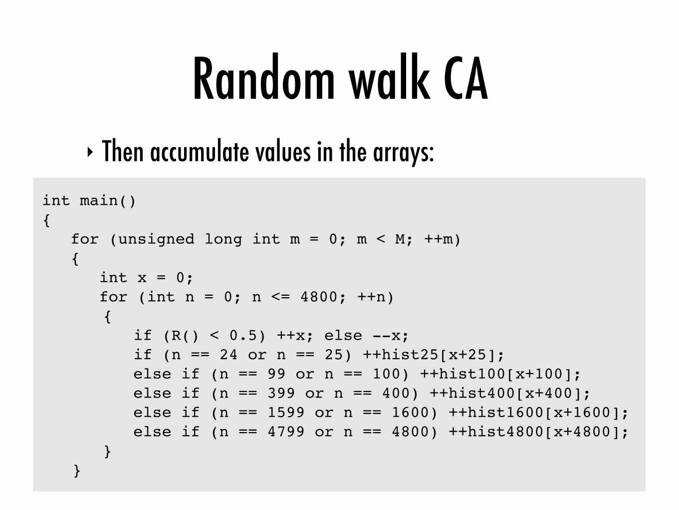
int main(){ for (unsigned long int m = 0; m < M; ++m) { int x = 0; for (int n = 0; n <= 4800; ++n)! ! {! ! ! if (R() < 0.5) ++x; else --x;! ! ! if (n == 24 or n == 25) ++hist25[x+25];! ! ! else if (n == 99 or n == 100) ++hist100[x+100];! ! ! else if (n == 399 or n == 400) ++hist400[x+400];! ! ! else if (n == 1599 or n == 1600) ++hist1600[x+1600];! ! ! else if (n == 4799 or n == 4800) ++hist4800[x+4800];! ! }! }
‣ Then accumulate values in the arrays:

Random walk CA
int main(){ for (unsigned long int m = 0; m < M; ++m) { int x = 0; for (int n = 0; n <= 4800; ++n)! ! {! ! ! if (R() < 0.5) ++x; else --x;! ! ! if (n == 24 or n == 25) ++hist25[x+25];! ! ! else if (n == 99 or n == 100) ++hist100[x+100];! ! ! else if (n == 399 or n == 400) ++hist400[x+400];! ! ! else if (n == 1599 or n == 1600) ++hist1600[x+1600];! ! ! else if (n == 4799 or n == 4800) ++hist4800[x+4800];! ! }! }
‣ Then accumulate values in the arrays:
watch theoffset!
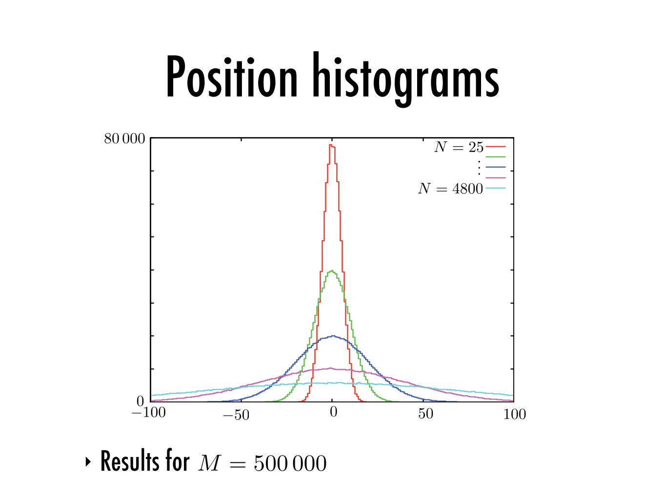
Position histograms
M = 500 000
N = 25
N = 4800
...
−100 −50 0 50 1000
80 000
‣ Results for

Asymptotic distribution
2M × e−x2/2σ
√πσ
×N
× 1
N
after rescaling,collapses onto

Asymptotic distribution‣ In the double limit , rescaled histogram is a
perfect gaussian (the normal distribution)
‣ Amazingly, a smooth, continuous distribution can result from a limiting sequence of discrete histograms
‣ Analogue of coarse-graining
‣ Rescaling implicitly turns integers into fractions; suggests that we can use rational numbers to cover the real line
N,M → ∞

Floating-point numbers‣ Floating-point numbers have the form
‣ The adjustable radix point allows for calculation over a wide range of magnitudes
‣ Floating-point numbers are limited by the number of bits used to represent the fraction and exponent
±f × be
fraction (or significand)
sign
base
exponent

Floating-point numbers‣ Real line is dense and uncountably infinite:
‣ FP scheme gives a partial covering:
x1 x2 R[x1, x2] �→ R
21 22 2127+0
−0
· · ·
inf
NaN
−inf
NaN

Floating-point numbers‣ Finite representation that manages to span many orders
of magnitude
‣ A sort of finite-precision scientific notation, with the significant and exponent encoded in fixed width binary
‣ Equal number of uniformly spaces values in each interval
‣ Relies on special values (+0, −0, inf, −inf, NaN)
[2n, 2n+1)

Floating point types
0 0 0 0 0 0 0 0 0 0 0 0 0 0 0 0 0 0 0 0 0 0 0 0 0 0 0 0 0 0 0 0
float
‣ Intel architecture follows the IEEE 754 standard
8-bit exponent field 23-bit fraction field
sign bit
0 0 0 0 0 0 0 0 0 0 0 0 0 0 0 0 0 0 0 0 0 0 0 0 0 0 0 0 0 0 0 0 0 0 0 0 0 ... 0
double
11-bit exponent field 52-bit fraction field
sign bit

Floating point types
0 0 1 1 1 1 1 1 1 0 0 0 0 0 0 0 0 0 0 0 0 0 0 0 0 0 0 0 0 0 0 0
float
‣ Representation of unity:
offset by 28−1 leading order 1 is hidden
sign bit
0 0 1 1 1 1 1 1 1 1 1 1 0 0 0 0 0 0 0 0 0 0 0 0 0 0 0 0 0 0 0 0 0 0 0 0 0 ... 0
double
offset by 211−1
sign bit

Floating point types
0 1 1 1 1 1 1 1 0 1 1 1 1 1 1 1 1 1 1 1 1 1 1 1 1 1 1 1 1 1 1 1
float
‣ Largest positive number:
all on state is reserved
sign bit
0 1 1 1 1 1 1 1 1 1 1 0 1 1 1 1 1 1 1 1 1 1 1 1 1 1 1 1 1 1 1111 1 1 1 1 1 ... 1
double
all on state is reserved
sign bit
leading order 1 is hidden

Floating point types
0 0 0 0 0 0 0 0 1 0 0 0 0 0 0 0 0 0 0 0 0 0 0 0 0 0 0 0 0 0 0 0
float
‣ Smallest positive non-denormalized number:
all off state is reserved
sign bit
0 0 0 0 0 0 0 0 0 0 0 1 0 0 0 0 0 0 0 0 0 0 0 0 0 0 0 0 0 0 0 0 0 0 0 0 0 ... 0
double
all off state is reserved
sign bit
leading order 1 is hidden
Floating point types
0 0 0 0 0 0 0 0 0 1 1 1 1 1 1 1 111 1 1 1 1 1 1 1 1 1 1 1 1 1 1
float
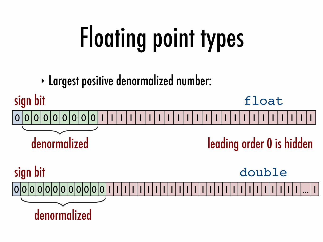
‣ Largest positive denormalized number:
denormalized
sign bit
0 0 0 0 0 0 0 0 0 0 0 0 1 1 1 1 1 1 1 1 1 111 1 1 1 1 1 1 1 111 111 111 1 ... 1
double
denormalized
sign bit
leading order 0 is hidden

Floating point types
1 0 0 0 0 0 0 0 0 0 0 0 0 0 0 0 0 0 0 0 0 0 0 0 0 0 0 0 0 0 0 0
float
‣ Negative zero:
denormalized
sign bit
1 0 0 0 0 0 0 0 0 0 0 0 0 0 0 0 0 0 0 0 0 0 0 0 0 0 0 0 0 0 0 0 0 0 0 0 0 ... 0
double
denormalized
sign bit
leading order 0 is hidden

Accuracy of FP arithmetic‣ FP arithmetic is by its nature inexact
‣ Important always to think about accuracy: should we believe the computer’s final answer?
‣ FP multiplication is relatively safe
‣ FP subtraction of nearly-equal quantities (or addition of equal magnitude, opposite sign quantities) can dramatically increase the relative error

Potential dangers
‣ FP operations can yield both “overflow” and “underflow”
‣ Additional notes on the class web site will explore the Infinity (Inf) and Not-a-Number (NaN) error states

Potential dangers‣ Associativity breaks down:
‣ The following 8-digit decimal floating point operation has a 5% relative error depending on the order in which operations are performed:
(11111113. +−11111111.) + 7.5111111 = 2.0000000 + 7.511111= 9.511111
11111113. + (−11111111. + 7.511111) = 11111113. +−11111103.
= 10.000000
(u + v) + w �= u + (v + w)
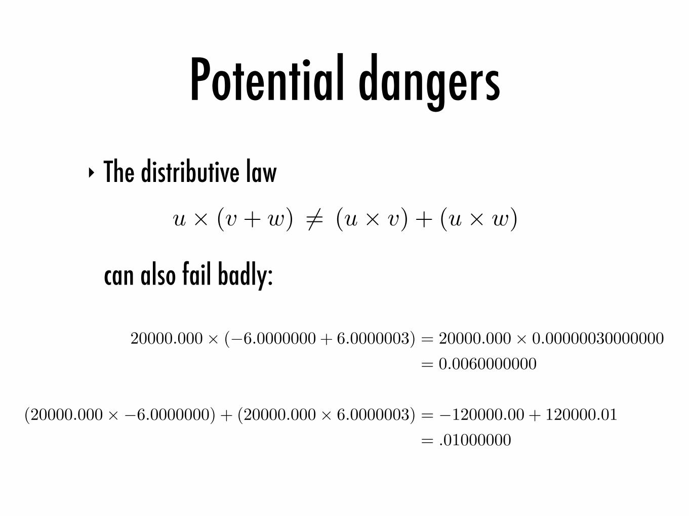
Potential dangers‣ The distributive law
can also fail badly:
u× (v + w) �= (u× v) + (u× w)
20000.000× (−6.0000000 + 6.0000003) = 20000.000× 0.00000030000000= 0.0060000000
(20000.000×−6.0000000) + (20000.000× 6.0000003) = −120000.00 + 120000.01= .01000000

Potential dangers
‣ It can easily occur that
‣ Hence, variance is not guaranteed to be positive
‣ Naively calculating the standard deviation can lead to your taking the square root of a negative number
σ =1n
����nn�
k=1
x2k −
� n�
k=1
xk
�2
2(u2 + v2) < (u + v)2

Potential dangers
‣ Many common mathematical relations no longer hold ...
(x + y)(x− y) = x2 − y2
sin2 θ + cos2 θ = 1

“Carefully written programs”
‣ technical meaning: programs that are numerically correct
‣ this is very difficult to guarantee!

“Carefully written programs”
‣ Which formula should we use to compute the average of x and y?
1. (x + y)/2
2. x/2 + y/2
3. x + ((y − x)/2)
4. y + ((x− y)/2)

“Carefully written programs”
1. (x + y)/2
2. x/2 + y/2
3. x + ((y − x)/2)
4. y + ((x− y)/2)
May raise an overflow if x and y have the same sign

“Carefully written programs”
1. (x + y)/2
2. x/2 + y/2
3. x + ((y − x)/2)
4. y + ((x− y)/2)
May degrade accuracy but is safe from overflows

“Carefully written programs”
1. (x + y)/2
2. x/2 + y/2
3. x + ((y − x)/2)
4. y + ((x− y)/2)May raise an overflow if x and y have opposite signs

“Carefully written programs”
‣ you want functions that are robust
‣ give some thought to the rare or extreme cases that may cause your function to misbehave
‣ avoid overflows and underflows
‣ avoid undefined operations, e.g.,√−1,
00

“Carefully written programs”
‣ Example: roots of the quadratic equation,
‣ According to the usual formula,
‣ Problem can arise if so that
‣ Cancellation can lead to catastrophic loss of significant digits:
ax2 + bx + c
x1,2 =−b±
√b2 − 4ac
2a
b2 � |4ac|�
b2 − 4ac ≈ |b|
b ± |b|2a
≈ 00

“Carefully written programs”‣ One possible workaround: use exact algebraic
manipulations on a per case basis
x1 =−b +
√b2 − 4ac
2a=
−2c
b +√
b2 − 4ac
x2 =−b−
√b2 − 4ac
2a=
2c
−b +√
b2 − 4ac

“Carefully written programs”‣ One possible workaround: use exact algebraic
manipulations on a per case basis
x1 =−b +
√b2 − 4ac
2a=
−2c
b +√
b2 − 4ac
x2 =−b−
√b2 − 4ac
2a=
2c
−b +√
b2 − 4ac
cancellation no cancellation

“Carefully written programs”#include <cassert>#include <cmath>using std::sqrt; // square rootusing std::fabs; // absolute value
void quadratic_roots(double a, double b, double c, double &x1, double &x2){ const double X2 = b*b-4*a*c; assert(X2 >= 0.0); const double X = sqrt(X2); const double Ym = -b-X; const double Yp = -b+X; const double Y = (fabs(Ym) > fabs(Yp) ? Ym : Yp);
x1 = 2*c/Y; x2 = Y/(2*a);}

“Carefully written programs”
‣ Example: norm of a complex number
‣ Avoid possible overflow when squaring terms:
z = x + iy, |z| =�
x2 + y2
|z| = x�
1 + r2, r =y
x, if |y| < |x|
|z| = y�
1 + r2, r =x
y, if |x| < |y|

“Carefully written programs”‣ Evaluation by nested polynomials (Horner’s scheme)f(x) = a0 + a1x+ a2x
2 + a3x3 + · · · aNxN
= a0 + x(a1 + x(a2 + x(a3 + · · ·x(aN−1 + xaN ) · · · )))
double eval_poly(const double f[], double x, int n){ double val = f[--n]; do { val *= x; val += f[--n]; } while (n != 0); return val;}

“Carefully written programs”#include <iostream>using std::cout;using std::endl;
int main(){ // f(x) = 1 + 20x + 9x^2 - 3x^3 // + 5x^4 + 2x^5 + x^6 double f[7] = { 1, 20, 9, -3, 5, 2, 1 }; for (int i = 0; i <= 1000; ++i) { const double x = (i-500)*3.0/500; cout << x << "\t" << eval_poly(f,x,7) << endl; } return 0;}

“Carefully written programs”
‣ Example: the sinc function
‣ possible problems as
‣ workaround: explicit power series expansion
sin(x)x
=x− x3
3! + x5
5! + · · ·x
= 1− x2
3!+
x4
5!+ · · ·
sin(x)x
x→ 0

Arbitrary precision arithmetic‣ scheme for performing operations on integers and
rational numbers with no rounding, e.g.,
‣ available in symbolic manipulation environments (Maple, Mathematica) and “bignum” libraries
‣ implemented in software; limited by system memory
21539932
+8717362
=1225057936559692