This document is the Pre-refereeing Manuscript version of a Published Work that appeared in final form in Journal of Physical Chemistry C, copyright © American Chemical Society after peer review and technical editing by the publisher. To access the final edited and published work see http://pubs.acs.org/doi/pdf/10.1021/jp505978p.

Floating Patches of HCN at the Surface of Their Aqueous

Solutions – Can They Make ‘HCN World’ Plausible?

Balázs Fábián,1,2 Milán Szőri3,* and Pál Jedlovszky1,4,5,*

1Laboratory of Interfaces and Nanosize Systems, Institute of Chemistry,

Eötvös Loránd University, Pázmány P. Stny 1/A, H-1117 Budapest,

Hungary

2Department of Inorganic and Analytical Chemistry, Budapest University

of Technology and Economics, Szt. Gellért tér 4, H-1111 Budapest,

Hungary

3Department of Chemical Informatics, Faculty of Education, University of

Szeged, Boldogasszony sgt. 6. H-6725 Szeged, Hungary

4MTA-BME Research Group of Technical Analytical Chemistry, Szt.

Gellért tér 4, H-1111 Budapest, Hungary

5EKF Department of Chemistry, Leányka utca 6, H-3300 Eger, Hungary

Running title: Surface of Aqueous HCN Solutions

e-mail: milan@jgypk.u-szeged.hu (M.Sz.), pali@chem.elte.hu (P.J.)

2

Abstract:

The liquid/vapor interface of the aqueous solutions of HCN of different concentrations

has been investigated using molecular dynamics simulation and intrinsic surface analysis.

Although HCN is fully miscible with water, strong interfacial adsorption of HCN is observed

at the surface of its aqueous solutions, and, at the liquid surface, the HCN molecules tend to

be located even at the outer edge of the surface layer. It turns out that in dilute systems the

HCN concentration can be about an order of magnitude larger in the surface layer than in the

bulk liquid phase. Furthermore, HCN molecules show a strong lateral self-association

behavior at the liquid surface, forming thus floating HCN patches at the surface of their

aqueous solutions. Moreover, HCN molecules are staying, on average, an order of magnitude

longer at the liquid surface than water molecules, and this behavior is more pronounced at

smaller HCN concentrations. Due to this enhanced dynamic stability, the floating HCN

patches can provide excellent spots for polymerization of HCN, which can be the key step in

the prebiotic synthesis of partially water soluble adenine. All these findings make the

hypothesis of ‘HCN World’ more plausible.

3

1. Introduction

Atmospheric hydrogen cyanide (HCN), a simple endothermic species, is produced

primarily in biomass burning as a result of pyrolysis of N-containing compounds. Although

the high natural variability in HCN emissions even within a single or similar fire types, it is

often used as a tracer of pollution originating from wildfires[!1-3] in order to deconvolute

mixtures of urban and biomass burning emissions.[!4] Besides biomass burning, atmospheric

HCN has also been formed in lightning perturbed air in the troposphere of the modern

Earth,[!5,6] making lightning an additional source of HCN.[!7] Considering the budget of

atmospheric HCN, its direct photolysis is apparently negligible; the estimated photochemical

lifetime of HCN is around 10 years or even more in the stratosphere below 30 km, and around

5 years in the upper troposphere.[!8] However, global satellite observations of HCN in the

upper troposphere[!9] reveal the clear signature of air depleted in HCN over the tropical

oceans.[!10] Therefore, the uptake into the ocean via wet deposition is currently known to be

the dominant sink with an inferred global HCN biomass burning source of 1.4–2.9 Tg(N)/year

and an oceanic saturation ratio of 0.83.[!11] Due to this oceanic loss, lifetime of HCN reduces

to 2-5 months,[!2,3,11] and it is thought to be an important source of nitrogen in remote

oceanic environments.[!11] Alternative stratospheric loss of HCN, in which reactions with

OH and O(1D) are dominated, can be assumed to be less pronounced.[!8,12]

The aforementioned formation of HCN by lightning does not only occur in the modern

atmosphere, but happened also in the atmosphere of prebiotic Earth. The pioneering

experiment by Miller and Urey,[!13] in which amino acids are readily formed from methane,

ammonia and water subjected to electric discharges, has naturally strengthened the

widespread assumption that the original formation of primitive proteins occurred through the

polycondensation of these monomers, although the amino acids are actually secondary

products arising from polypeptides formed by way of polymerization of HCN.[!14,15] Such

formation of HCN is not unique feature of the Miller-Urey setup, it can be occurred by

electric discharges from many diverse mixtures of gases, including, CO-N2-H2, and CO2-N2-

H2O.[!16,17] Therefore, HCN is considered to have been an important source of biological

molecules on the primitive Earth.[!18-22] After the uptake of HCN in water, two chemical

processes are assumed to occur: the polymerization (probably to biomolecules) and the

hydrolysis of HCN to NH2CHO. Generally speaking, the hydrolysis predominates in dilute

solutions, while polymerization takes over at higher concentrations.[!23] Oligomerization of

4

HCN is of particular interest because adenine is an essential nucleobase and formally it is the

pentamer of HCN.[!16,24,25] Several amino acids and peptides can also be synthesized

through the oligomerization of HCN followed by hydrolysis, which supports the hypothesis of

the so-called ‘HCN world’.[!15,26] Nevertheless, adenine can be detected only in

concentrated (1-11 M) aqueous solutions of HCN.[!27,28] Thus, the main criticism

concerning the ‘HCN world’ hypothesis is that the bulk concentration of HCN in the primitive

ocean was estimated to be far too low for polymerization, and hence hydrolysis to NH2CHO

could have been favored instead.[!29,30] Based solely on this evidence, it is less plausible that

prebiotic formation of the biomolecular building blocks via the oligomerization could happen

in the bulk phase due to the issue with HCN concentration. Air/ice[!31] and air/water

interfaces can, however, be alternative locations for possible enrichment of HCN where

oligomerization could have taken place. Due to the fact that HCN is a highly water soluble

weak acid, only its bulk phase properties are usually considered. It was shown recently that

molecular HCl, which possesses strong acidity, have a very strong propensity for the air-water

interface.[!32] The question can thus be arisen that HCN has also significant enrichment at the

surface of its aqueous solution regardless to its weaker acidic character.

Computer simulation methods seem to be particularly suitable to address this question,

since in a computer simulation a full, atomistic level insight is gained to the structure of the

appropriately chosen model of the system of interest. However, when the surface of a liquid

phase is seen at atomistic resolution, as is in computer simulations, the detection of the exact

location of the liquid surface (or, equivalently, the distinction between interfacial and non-

interfacial molecules) is far from being a trivial task. The problem originates from the fact

that the liquid surface is corrugated by capillary waves at the atomistic length scale. Defining

the interface simply as a slab parallel with its macroscopic plane, as done in many of the early

simulations, is repeatedly shown to lead to systematic error of unknown magnitude not only in

the structural properties of the interface, [!33,34] but also in its composition (i.e., extent of

adsorption of certain components) [!35-37] and even in some of the thermodynamic

properties of the system. [!38] To overcome this problem several methods have been

proposed in the past decade, [!33,39-43] among which the method called Identification of the

Truly Interfacial Molecules (ITIM) [!33] turned out to be an excellent compromise between

computing time and accuracy. [!44] The ITIM method has successfully been applied to

describe the liquid-vapor interface of various aqueous mixtures [!35-37,45] as well as that of

other systems [!33,46-50] and various water-organic liquid-liquid interfaces. [!34,38,51,52] It

has also been used to calculate the intrinsic solvation free energy profile (i.e., that relative to

5

the real, capillary wave corrugated liquid surface) of various penetrants across liquid-liquid

interfaces, [!53,54] and proved to be essential in explaining the surface tension anomaly of

neat water. [!55]

In this paper we present computer simulation results of the liquid-vapor interface of

water-HCN mixtures of six different compositions, covering the HCN mole percentage range

from 3 to 30%. As it turns out, due to the strong adsorption of HCN at the liquid surface these

systems practically cover the entire composition range for the surface layer. For reference,

simulations of the two neat systems are also reported here. The surface layer of the liquid

phase is identified in the simulations by means of the ITIM method, and its properties (i.e.,

width, roughness, orientation of the surface molecules, adsorption and lateral self-association

of HCN in the surface layer, dynamics of exchange of the molecules between the surface

layer and the bulk liquid phase) are analyzed in detail. Particular emphasis is given to

properties that can be relevant in respect of a possible HCN oligomerization at the surface of

its dilute aqueous solution. The results obtained for the first molecular layer beneath the liquid

surface is also compared to those obtained for the subsequent subsurface molecular layers.

The paper is organized as follows. In section 2 details of the computer simulations and

ITIM analyses performed are given. The obtained results, concerning both the properties of

the entire surface layer and also those of the molecules belonging to it are presented and

detailed in section 3. Finally, in section 4 the main conclusions of this study are summarized,

and the relevance of the present results in respect of the possible polymerization of HCN

under prebiotic conditions is addressed.

2. Computational Details

Molecular dynamics simulation of the liquid-vapor interface of water-HCN mixtures

of different compositions have been performed on the canonical (N,V,T) ensemble at the

temperature of 273 K. The X, Y and Z edges of the rectangular basic simulation box have been

300, 50 and 50 Å, respectively; edge X has been perpendicular to the macroscopic plane of the

interface. Standard periodic boundary conditions have been applied. The basic box has

consisted of 4000 molecules, among which 0, 120, 200, 400, 600, 800, 1200, and 4000 have

been HCN in the different simulations. These systems are referred to here as the 0% HCN,

3% HCN, 5% HCN, 10% HCN, 15% HCN, 20% HCN, 30% HCN, and 100% HCN system,

respectively.

6

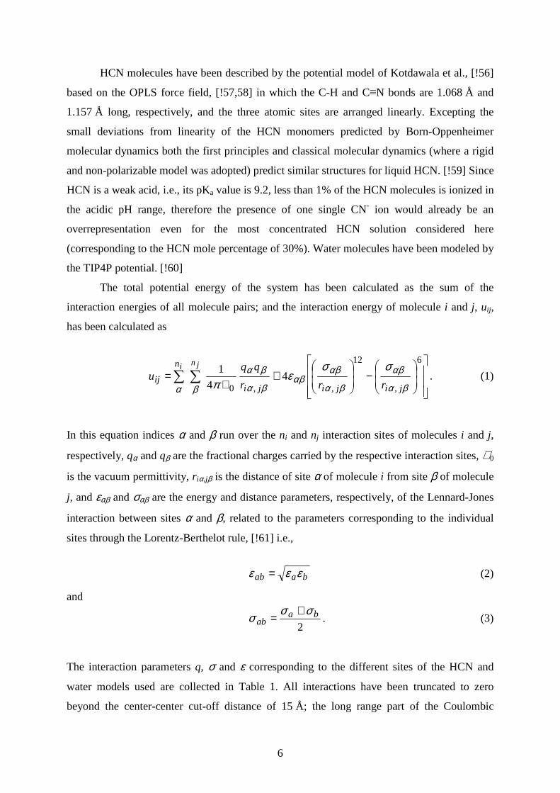
HCN molecules have been described by the potential model of Kotdawala et al., [!56]

based on the OPLS force field, [!57,58] in which the C-H and C≡N bonds are 1.068 Å and

1.157 Å long, respectively, and the three atomic sites are arranged linearly. Excepting the

small deviations from linearity of the HCN monomers predicted by Born-Oppenheimer

molecular dynamics both the first principles and classical molecular dynamics (where a rigid

and non-polarizable model was adopted) predict similar structures for liquid HCN. [!59] Since

HCN is a weak acid, i.e., its pKa value is 9.2, less than 1% of the HCN molecules is ionized in

the acidic pH range, therefore the presence of one single CN- ion would already be an

overrepresentation even for the most concentrated HCN solution considered here

(corresponding to the HCN mole percentage of 30%). Water molecules have been modeled by

the TIP4P potential. [!60]

The total potential energy of the system has been calculated as the sum of the

interaction energies of all molecule pairs; and the interaction energy of molecule i and j, uij,

has been calculated as

∑ ∑

−

+

∈=

i jnn

jijijiij rrr

qqu

α β βα

αβ

βα

αβαβ

βα

βα σσε

π

6

,

12

,,04

4

1. (1)

In this equation indices α and β run over the ni and nj interaction sites of molecules i and j,

respectively, qα and qβ are the fractional charges carried by the respective interaction sites, ∈0

is the vacuum permittivity, r iα,jβ is the distance of site α of molecule i from site β of molecule

j, and εαβ and σαβ are the energy and distance parameters, respectively, of the Lennard-Jones

interaction between sites α and β, related to the parameters corresponding to the individual

sites through the Lorentz-Berthelot rule, [!61] i.e.,

baab εεε = (2)

and

2ba

abσσσ +

= . (3)

The interaction parameters q, σ and ε corresponding to the different sites of the HCN and

water models used are collected in Table 1. All interactions have been truncated to zero

beyond the center-center cut-off distance of 15 Å; the long range part of the Coulombic

7

interaction of the fractional charges has been taken into account by the Particle Mesh Ewald

(PME) method. [!62]

The simulations have been performed by the GROMACS 4.5.5 program package.

[!63] The temperature of the system has been controlled using the Nosé-Hoover thermostat.

[!64,65] According to the potential models used, both the HCN and the water molecules have

been treated as rigid bodies in the simulations; their geometries have been kept unchanged by

means of the LINCS [!66] and SETTLE [!67] algorithms, respectively. The equations of

motion have been integrated in time steps of 1 fs. Initial configurations have been created in

the following way. First, the required number of molecules have been placed in a basic box

the Y and Z edges of which have already been 50 Å, while the length of the X edge has

roughly corresponded to the density of the liquid phase. After proper energy minimization the

systems have been equilibrated for 2 ns on the isothermal-isobaric (N,p,T) ensemble at 1 bar.

The liquid-vapor interface has then been created by increasing the length of the X edge to

300 Å. The interfacial system has been further equilibrated, already on the (N,V,T) ensemble,

for another 2 ns. Finally 2000 sample configurations, separated by 1 ps long trajectories each,

have been dumped for further analyses during the 2 ns long production stage of the

simulations. The surface tensions of the systems studied are collected in Table 2, as obtained

from the simulations.

The molecules constituting the first layer of the liquid phase have been identified by

means of the ITIM method, [!33] i.e., by moving a probe sphere along test lines perpendicular

to the macroscopic plane of the interface, YZ, from the bulk vapor phase towards the interface.

The molecules that are first hit by the probe sphere along any of the test lines (i.e., the ones

‘seen’ by the probe from the vapor phase) are considered as being at the interface. Test lines,

being parallel with edge X of the basic box have been arranged in a 100×100 grid along the

YZ plane, thus, two neighboring test lines have been separated by 0.5 Å. According to the

suggestion of Jorge et al., [!44] the radius of the probe sphere has been set to 1.25 Å. To

determine when a molecule is touched by the probe the atoms have been approximated by

spheres, the diameters of which have been equal to the corresponding Lennard-Jones distance

parameter, σ. This way, H atoms have been omitted from the ITIM analysis (see Table 1).

Finally, by disregarding the molecules identified as forming the surface layer and repeating

the entire procedure twice more the molecules forming the second and the third layer beneath

the liquid surface have also been identified. An equilibrium snapshot of the 20% HCN

system, indicating also the molecules forming the first three subsurface molecular layers as

identified by ITIM, is shown in Figure 1.

8

3. Results and Discussion

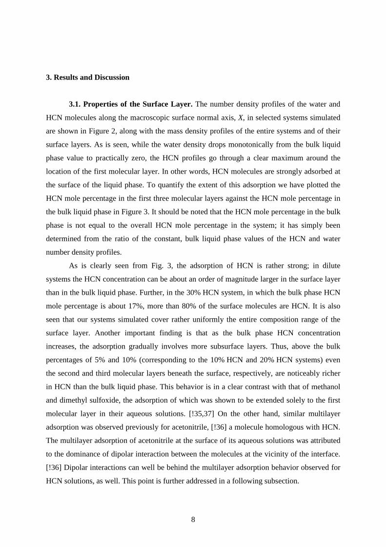
3.1. Properties of the Surface Layer. The number density profiles of the water and

HCN molecules along the macroscopic surface normal axis, X, in selected systems simulated

are shown in Figure 2, along with the mass density profiles of the entire systems and of their

surface layers. As is seen, while the water density drops monotonically from the bulk liquid

phase value to practically zero, the HCN profiles go through a clear maximum around the

location of the first molecular layer. In other words, HCN molecules are strongly adsorbed at

the surface of the liquid phase. To quantify the extent of this adsorption we have plotted the

HCN mole percentage in the first three molecular layers against the HCN mole percentage in

the bulk liquid phase in Figure 3. It should be noted that the HCN mole percentage in the bulk

phase is not equal to the overall HCN mole percentage in the system; it has simply been

determined from the ratio of the constant, bulk liquid phase values of the HCN and water

number density profiles.

As is clearly seen from Fig. 3, the adsorption of HCN is rather strong; in dilute

systems the HCN concentration can be about an order of magnitude larger in the surface layer

than in the bulk liquid phase. Further, in the 30% HCN system, in which the bulk phase HCN

mole percentage is about 17%, more than 80% of the surface molecules are HCN. It is also

seen that our systems simulated cover rather uniformly the entire composition range of the

surface layer. Another important finding is that as the bulk phase HCN concentration

increases, the adsorption gradually involves more subsurface layers. Thus, above the bulk

percentages of 5% and 10% (corresponding to the 10% HCN and 20% HCN systems) even

the second and third molecular layers beneath the surface, respectively, are noticeably richer

in HCN than the bulk liquid phase. This behavior is in a clear contrast with that of methanol

and dimethyl sulfoxide, the adsorption of which was shown to be extended solely to the first

molecular layer in their aqueous solutions. [!35,37] On the other hand, similar multilayer

adsorption was observed previously for acetonitrile, [!36] a molecule homologous with HCN.

The multilayer adsorption of acetonitrile at the surface of its aqueous solutions was attributed

to the dominance of dipolar interaction between the molecules at the vicinity of the interface.

[!36] Dipolar interactions can well be behind the multilayer adsorption behavior observed for

HCN solutions, as well. This point is further addressed in a following subsection.

9

Comparing the mass density profiles of the entire systems with those of the first layers

(Fig. 2) it is seen that the first layer density peak extends well beyond the point where the

density of the entire system already reaches the constant, bulk liquid phase value. This means

that defining the interfacial region in the non-intrinsic way, i.e., as a slab of intermediate

densities, would miss a large number of truly interfacial molecules (i.e., what can be seen

from the vapor phase). Conversely, as seen from Figure 4, which shows the mass density

profiles of the first three molecular layers along with that of the entire system in four selected

mixed systems, the density peak of the second, and even that of the third layer overlaps with

the intermediate density part of the profile of the whole system. Thus, besides missing a large

number of interfacial molecules, the non-intrinsic treatment of the interface would also

misidentify a large number of molecules as being interfacial.

The density peaks corresponding to the individual subsurface molecular layers can be

very well fitted by a Gaussian function in every case. Since the density profiles of the

consecutive molecular layers are indeed supposed to follow Gaussian distributions, [!70] this

finding confirms the proper choice of the probe sphere radius in the ITIM analysis. [!44] The

width parameter of the fitted Gaussian function, δ, can serve as a measure of the width of the

corresponding molecular layer, whereas the position of its center, Xc, is an estimate of the

position of this layer. Thus, the difference of the Xc values of two consecutive layers, ∆Xc,

characterizes the average separation of these layers. The δ and Xc values corresponding to the

first three layers of the systems simulated are collected in Table 3. It is seen that, unlike in

neat water, the first layer is always noticeably wider than the subsequent ones in HCN

solutions, and this difference increases from about 2-3% to 6-8% with increasing HCN

concentration. On the other hand, no tendentious difference is seen between the widths of the

second and third subsurface molecular layers. Further, with increasing HCN concentration all

the three subsurface layers become wider, as seen from the 20-30% increase of the

corresponding δ parameters upon going from dilute to concentrated solutions. Similarly, the

separation of the first two layers is always larger than that of the second and third layers, and

this difference increases from about 3% to 10% upon going from dilute to concentrated

solutions. Further, not only the difference between the separations of the first and second, and

that of the second and third layers (i.e., ∆Xc(1-2) - ∆Xc(1-3)) increases with increasing HCN

content, but also these inter-layer separations (i.e., the ∆Xc values) themselves. All these

findings indicate that the molecules are less tightly packed at the liquid surface than in the

bulk liquid phase, and this effect is more pronounced around the HCN than around the water

10

molecules. The reason for this less compact arrangement of the molecules at the interface is

probably related to the fact that the orientational preferences of these molecules imposed by

the vicinity of the vapor phase is not fully compatible with their tightly packed arrangement,

which dominates in the bulk phase. The point concerning the interfacial orientation of the

molecules is addressed in detail in a subsequent subsection.

Figure 5 compares the number density profiles of the water and HCN molecules in the

surface layer of four selected mixed systems. The position of the molecules has been

estimated by that of their O and C atoms, respectively. For better comparison, the two profiles

are always scaled to each other. As is clear, the density peak of the HCN molecules is always

shifted by 1.7-2.0 Å towards the vapor phase, as compared with the water density peak. This

finding indicates that HCN is not only adsorbed at the first few molecular layers beneath the

liquid surface, but even within the surface layer they are located noticeably closer to the vapor

phase than the water molecules.

The ITIM algorithm not only identifies the full list of the surface molecules, but can

also provide a set of points that can serve as an estimate of the geometric covering surface of

the liquid phase. This set of points can be determined from the positions the probe sphere is

stopped along the different test lines. [!33] Having the covering surface of the liquid phase

already determined, its roughness can also be characterized. However, the description of the

roughness of a known wavy surface is still not a trivial task, and it requires the use of at least

two independent parameters, i.e., an amplitude-like and a frequency-like one. [!33] For this

purpose, we proposed to use the following parameter pair. [!45] The average normal distance

(i.e., distance along the macroscopic surface normal axis, X) of two surface points, d ,

exhibits a saturation curve as a function of their lateral distance, l (i.e., distance in the

macroscopic surface plane, YZ). The )(ld data can be well fitted by the function

la

lald

ξξ

+=)( . (4)

The parameters ξ and a, corresponding to the steepness of the )(ld curve at small, and to its

saturation value at large l values, respectively, can then serve as the frequency-like and

amplitude-like roughness parameter, respectively. We have recently shown that the

amplitude-like parameter, a, defined this way is closely related to the surface tension of the

system. [!71]

11

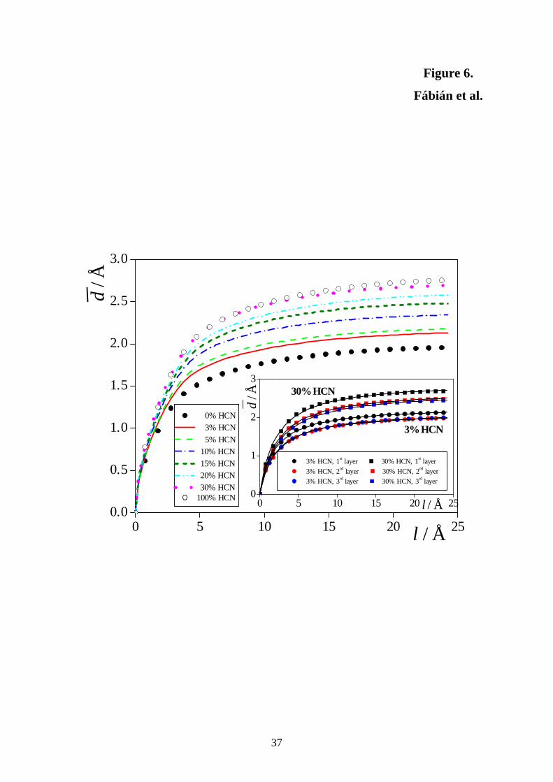
The )(ld roughness curves obtained in the systems simulated are shown in Figure 6,

whereas the a and ξ parameters corresponding to all the three subsurface layers are collected

in Table 3. As is seen, with increasing HCN concentration the liquid surface gets rougher both

in terms of frequency and amplitude, as the ξ and a parameters increase by about 15% and

30%, respectively, upon going from neat water to neat HCN. It is also seen that the surface

layer is always somewhat rougher than the subsequent molecular layers, as the ξ parameter is

about 15%, whereas a is about 8-10% larger in the first than in the second and third layer in

every case. On the other hand, no considerable difference is seen between the roughness of

the second and third layers in any case. This finding is illustrated by the inset of Fig. 6,

showing the )(ld data in the first three layers of the 3% HCN and 30% HCN systems,

together with the curves fitted to them according to eq. 4. The findings that (i) increasing

HCN content leads to an increased roughness of the liquid surface, and (ii) the first layer is

always rougher than the subsequent ones are perfectly in line with our previous observations

concerning the width and separation of the subsequent molecular layers, and stress again that

the molecules are less tightly packed at the liquid surface than in the bulk liquid phase, and

this effect is more pronounced for the HCN than for the water molecules.

3.2. Lateral Self-Association of the Surface Molecules. We have seen that HCN

molecules are strongly adsorbed, i.e., their local concentration is considerably increased at the

surface of their dilute aqueous solutions. Local HCN concentration can further increase within

the surface layer by possible lateral self-association of the like molecules. Self-association in

binary mixtures can be conveniently studied by Voronoi analysis. [!72-74] In two dimensional

systems (e.g., liquid surfaces) of discrete seeds (e.g., molecules) the Voronoi polygon (VP) of

a given seed is the locus of the points that are closer to this seed than to any other one.

Further, the VP edges and vertices are loci of points having two and three closest seeds,

respectively, at equal distances. Therefore, VP vertices are the centers of the largest circular

vacancies (i.e., circles not containing any seed) in the system. [!75,76] It has been shown that

in the case of uniformly distributed seeds the distribution of the VP area, A, (or, in three

dimensions that of the VP volume) is of Gaussian shape, whereas in cases when the seeds

show large local density fluctuations the VP area distribution exhibits a long tail of

exponential decay at large areas. [!77] Taking this property into account self-association in

binary mixtures can be detected in the following way. [!78] First, the VP area distribution of

all the seeds (molecules) is determined, to check that the molecules, irrespective of their type,

12

are indeed uniformly distributed at the surface. Then the VP area distribution is determined

considering only one of the two components in the analysis, and completely disregarding the

molecules of the other component. In case of self-association of the disregarded component

the area occupied by such self-aggregates is transformed into voids, and the VP area

distribution of the component considered exhibits the exponential tail. This method has been

successfully applied to detect self association several times, both in two- [!35-37] and three-

dimensional [!78,79] systems.

To investigate the possible self-association behavior of HCN molecules at the surface

of their aqueous solutions we have projected the centers (i.e., C or O atom) of all surface

molecules to the macroscopic plane of the interface, YZ, and performed Voronoi analysis by

considering both components as well as by disregarding one of them. The VP area

distributions are shown in Figure 7 as obtained in selected systems. To emphasize the

exponential character of the decay of the large area tails the distributions are shown on a

logarithmic scale. As is evident, there is a marked difference between the shape of the P(A)

distributions obtained by taking both components into account and by disregarding one of the

components. In the first case P(A) is a narrow Gaussian, indicating, as expected, that surface

molecules are uniformly distributed along the macroscopic plane of the surface. In the second

case, however, the P(A) distribution becomes very broad and exhibits an exponentially

decaying tail (converted to a straight line by the logarithmic scale used) at large A values. It is

also seen that the smaller the concentration of a given component is in the surface layer, the

broader its P(A) distribution becomes. All these results indicate clearly that like components

exhibit a strong tendency of self-association at the liquid surface of aqueous HCN solutions,

and this self-association tendency is stronger for components of smaller concentration. The

observed self-association behavior of the like molecules is illustrated in Figure 8, showing

equilibrium snapshots of the surface layer of systems of three different compositions by

projecting the center of the surface molecules to the macroscopic plane of the surface, YZ.

Considering our above finding that surface HCN molecules tend to stay at the outer edge of

the surface layer, the lateral self-associates of the surface HCN molecules can be regarded as

patches floating at the surface of the liquid phase.

To quantify the extent of this self-association one can determine the area of the largest

circular voids when HCN molecules are disregarded from the analysis (as these voids are the

surface portions that are covered by HCN self-aggregates), and compare this value to the

average area occupied by a single HCN molecule (i.e., the mean value of P(A)) as obtained in

the 100% HCN system. Having these values calculated it turns out that HCN self-aggregates

13

may consist up to 8, 12, 25, 35, 55 and 150 molecules in the 3% HCN, 5% HCN, 10% HCN,

15% HCN, 20% HCN and 30% HCN systems, i.e., when the bulk phase HCN concentration

is about 0.8, 1.5, 2.8, 4.5, 5.5, and 8 M, respectively.

3.3. Dynamics of Exchange of the Molecules between the Surface and the Bulk.

The dynamics of exchange of the molecules between the surface layer and bulk of the liquid

phase can be characterized by the survival probability of the molecules in the surface layer,

L(t), i.e., the probability that a molecule that belongs to the surface layer at t0 will stay at the

surface up to t0 + t. In order to distinguish between the situations when the molecule leaves

the surface permanently, and when it is only absent from the surface at a certain instant due to

an oscillating move, departure of a molecule from the surface layer is allowed between t0 and

t0 + t, given that it returns to the surface layer within ∆t. Taking into account the typical time

scale of such molecular oscillations, ∆t is set here to its conventionally used value of 2 ps.

Considering also that two consecutive sample configurations are always separated by an 1 ps

long trajectory, this choice of ∆t practically means that molecules are considered as left the

surface layer if they are absent from this layer in two consecutive sample configurations. To

avoid any possible arbitrariness corresponding to the particular choice of ∆t, we have repeated

all the calculations with the ∆t value of 1 ps (i.e., when the definition does not allow the

molecules to be out of the surface layer even in a single sample configuration), but it did not

change any of the conclusions of this analysis.

Since the permanent departure of the molecules from the surface layer is a process of

first order kinetics, the L(t) data can be very well fitted by the exponentially decaying function

exp(-t/τ), where τ is the mean residence time of the molecules at the surface.

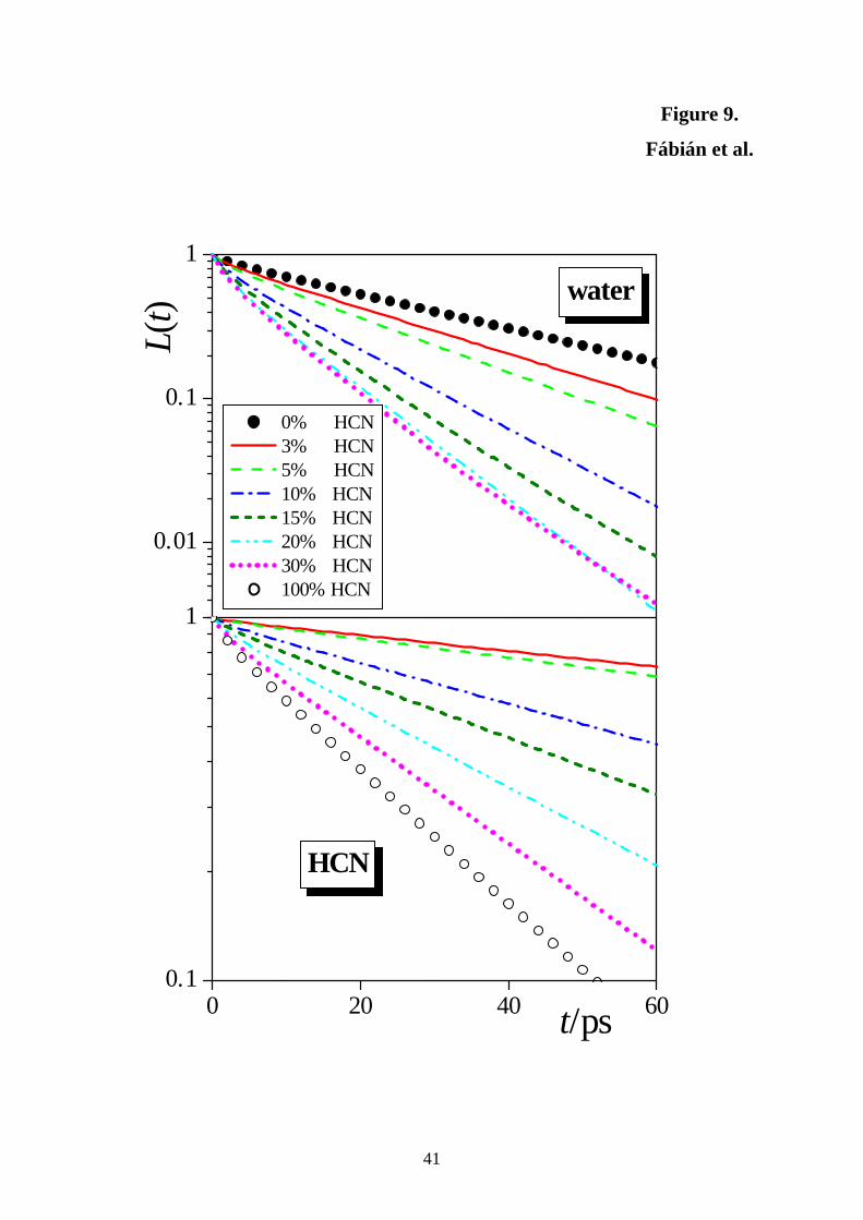
The L(t) survival probabilities of the water and HCN molecules in the surface layer of

the different systems simulated are shown in Figure 9, whereas the τ values corresponding to

the first three subsurface molecular layers are included in Table 3. To emphasize the

exponential decay of the survival probability, Fig. 9 shows the obtained L(t) data on a

logarithmic scale. As is immediately seen, the τ values in the second and third layers are

always an order of magnitude smaller than in the first layer, being comparable with the time

window of ∆t = 2 ps used in the analysis, indicating that defining the residence time in the

second and subsequent molecular layers is physically already meaningless. In other words, the

vicinity of the interface affects solely the first molecular layer beneath the liquid surface in

14

this respect, whereas, from the dynamical point of view, the second subsurface molecular

layer already belongs to the bulk liquid phase.

More importantly, it is seen that HCN molecules stay, on average, considerably longer

at the liquid surface than the water molecules, and this difference is larger when the solution

is more dilute. Thus, in the 3% HCN system the mean residence time of the HCN molecules

at the surface is about 8 times larger than that of the water molecules, whereas this ratio is

only about 3 in the 30% HCN system. The mean residence time of the water molecules at the

surface decreases parallel with that of the HCN molecules as the HCN concentration of the

system increases. Thus, the presence of HCN speeds up the dynamics of exchange of the

water molecules between the surface layer of the liquid phase and the bulk. These results

indicate that in dilute solutions the HCN molecules are not only strongly adsorbed at the

liquid surface, staying preferably at the outer edge of the surface layer, and exhibit strong

lateral self-association resulting in large interfacial HCN clusters, but also stay for unusually

long time, an order of magnitude longer than water molecules, at the surface of the liquid

phase. In other words, the floating patches of HCN are rather stable, staying at the liquid

surface for rather long time.

3.4. Surface Orientation. The orientation of a rigid molecule of general shape relative

to an external direction (or plane) can only be described by two orientational variables,

whereas that of molecules of C∞v symmetry (e.g., linear ones) can already be described by one

single variable. Therefore, the orientational statistics of the water molecules can be fully

characterized only by the bivariate joint distribution of two independent orientational

parameters, [!80,81] while that of HCN can simply be described by the monovariate

distribution of one single orientational parameter. For molecules of general shape we have

shown that the polar angles ϑ and φ of the macroscopic surface normal axis, X, pointing, by

our convention, towards the vapor phase, in a local Cartesian frame fixed to the individual

molecules represent a sufficient choice of such a parameter pair. [!80,81] Here we define this

local Cartesian frame of the water molecules in the following way. Its axis x is the molecular

normal axis, axis y is parallel with the line joining the two H atoms, and axis z is the main

symmetry axis of the molecule, directed to point from the O atom towards the H atoms along

the molecular dipole vector. Due to the C2v symmetry of the water molecule, this frame can

always be chosen in such a way that the angle φ does not exceed 90o. Further, since ϑ is an

angle of two general spatial vectors, but φ is formed by two vectors restricted to lay in a given

15

plane (i.e., the xy plane of the molecular frame) by definition, uncorrelated orientation of the

molecules with the surface plane results in constant distribution only if cosϑ and φ are chosen

to be the orientational variables. In the case of HCN the situation is considerably simpler, here

we characterize the orientational statistics of the surface HCN molecules by the cosine

distribution of the angle γ, formed by the vector pointing from the H to the N atom of the

molecule and the macroscopic surface normal vector, X, pointing from the liquid to the vapor

phase. The definition of the local Cartesian frame fixed to the individual water molecules as

well as that of the angles ϑ, φ and γ are illustrated in Figure 10.a.

It has been shown several times that the orientational preferences of the surface

molecules strongly depend on the local curvature of the surface. [!33-38,82] To take this

effect also into account we have divided the surface layer to three separate zones, marked by

A, B and C. Thus, zones A and C extend from the points where the mass density of the

surface layer is half of its maximum value towards the vapor and the liquid phase,

respectively, whereas zone B covers the X range where the mass density of the surface layer

exceeds half of its maximum value. Thus, zones A and C typically cover the crests and

troughs of the wavy liquid surface, i.e., surface portions of locally convex and concave

curvature, respectively. The division of the surface layer into zones A, B and C is illustrated

in Figure 10.b.

The P(cosϑ,φ) orientational maps of the water molecules and the P(cosγ) orientational

distributions of the HCN molecules are shown in Figures 11 and 12, respectively, as obtained

in selected systems simulated. As it has been shown several times, [!33,34] the molecules at

the surface of neat water prefer to lay parallel with the plane of the macroscopic surface, as

evidenced by the peak of the P(cosϑ,φ) orientational map at cosϑ = 0 and φ = 0o. This

preferred orientation is marked here by I. In zones A and C the peak corresponding to

orientation I shifts to somewhat smaller (in zone A) and larger (in zone C) cosϑ values,

indicating that the water molecules prefer slightly tilted orientations, pointing by their H

atoms flatly towards the bulk liquid phase in zone A and towards the vapor phase in zone C.

These orientations are marked here as IA and IC. Further, in both of these zones another

orientation, characterized by the cosϑ value of 0.5 (in zone A) and -0.5 (in zone C), and the φ

value of 90o is preferred. In these orientations, denoted by II and III, respectively, the water

molecule stays perpendicular to the macroscopic plane of the surface, pointing by one of its

O-H bonds straight towards the vapor phase (in zone A) and towards the bulk liquid phase (in

zone C). These orientational preferences have been rationalized by considering that in zone A

16

both preferred orientations are such that the water molecule “sacrifices” one of its four

hydrogen bonding directions (i.e., a lone pair direction in alignment IA and an O-H direction

in alignment II), and, on this, price it can form three stable hydrogen bonds in the other three,

inward-oriented directions. On the other hand, in the orientations preferred in zone C three

hydrogen bonding directions (i.e., one lone pair and two O-H directions in alignment IC, and

one O-H and two lone pair directions in alignment III) are straddling along the locally

concave surface, maintaining thus all the four hydrogen bonds of the water molecule. [!33,34]

As is seen from Fig. 11, in the presence of even a small amount of HCN the preference

for orientations II and III already vanishes, and the water molecules prefer nearly parallel

alignment with the macroscopic surface plane everywhere within the surface layer.

Correspondingly, the HCN molecules also prefer to lay almost parallel with the macroscopic

plane of the surface, declining only by about 5-10o from it (see Fig. 12). The only exception is

zone C, where the N atom of the HCN molecule sticks preferentially out to the vapor phase.

The preferred parallel alignment of both the water and the HCN molecules with the

macroscopic surface plane allows strong dipolar interactions acting between neighbors within

the surface layer, which can also explain the disappearance of the preference of the water

molecules for the perpendicular alignments II and III.

To confirm the presence of considerable dipolar interactions within the surface layer,

we have calculated the cosine distribution of the angle α, formed by the HN vector of two

neighboring HCN molecules in the surface layer. (Two HCN molecules are regarded to be

neighbors if their C atoms are closer than 6.0 Å, i.e., the first minimum position of the

corresponding radial distribution function. [!31]) The obtained P(cosα) distributions, shown

in Figure 13, exhibit their main peak at cosα = 1, indicating the clear preference of the

neighboring HCN molecules for parallel relative alignment. Further, a small peak of P(cosα)

is seen at the cosα value of -1, being larger in more dilute systems, indicating the secondary

preference of the neighboring HCN molecules for antiparallel relative alignment. All these

orientational preferences are illustrated in Figure 14.

The observed preferred relative alignment of the neighboring surface HCN molecules

is in a full accord with the assumed strong dipolar interactions within the surface layer. These

dipolar interactions can further stabilize the HCN patches floating at the liquid surface, and

can be, at least partly, be responsible for the unusually long residence time of the HCN

molecules in the surface layer.

17

4. Summary and Conclusions

In this paper we presented a detailed investigation of the intrinsic surface of aqueous

HCN solutions of different concentrations by means of molecular dynamics computer

simulation and ITIM analysis. One of the most important findings of this study is that HCN

molecules are strongly adsorbed at the surface of the liquid phase despite the full miscibility

of HCN with water. Thus, in dilute solutions even about an order of magnitude larger HCN

concentrations can be found at the surface layer than in the bulk liquid phase. In addition, the

larger the bulk phase HCN concentration is, the more subsurface layers are involved in HCN

adsorption, resulting in significant enrichment of HCN also in the second and third subsurface

molecular layers as compared to the bulk liquid phase. Another interesting feature of the

surface HCN molecules is that they prefer to stay at the outer edge of the surface layer, being

noticeably closer to the vapor phase than the surface water molecules. Also, all the three

subsurface layers become wider with increasing HCN concentration. As a consequence of this

chaotropic nature of HCN, the molecules are less tightly packed at the liquid surface than in

the bulk liquid phase, and hence the liquid surface gets rougher with increasing HCN

concentration.

Besides the aforementioned strong adsorption, the local HCN concentration is found to

be even further increased at certain patches of the liquid surface by the strong self-association

tendency of the like molecules, detected by Voronoi analysis of the surface layer.

Furthermore, the mean residence time of the HCN molecules at the liquid surface is found to

be considerably longer than that of the water molecules, and the more dilute the solution is,

the longer can HCN molecules stay at the liquid surface. All these findings indicate that the

HCN molecules can form long-lasting HCN patches floating at the surface of their aqueous

solutions, even at low bulk phase concentrations.

This finding has important consequences regarding to the ‘HCN World’ hypothesis,

[!15,26] the main argument against which is that polymerization of HCN and thus the

formation of adenine can only occur in concentrated (1-11 M) solutions. [!27,28] The present

results show, however, that HCN concentration can be very high at certain patches of even its

dilute aqueous solutions, and such floating HCN patches can be considered to have formed by

spontaneous process in the primordial time. These floating HCN patches might provide spots

for polymerization of HCN, which could finally lead to the dawn of the prebiotic

biomolecular building blocks, such as adenine. Therefore, adenine might well form at the

18

surface of dilute HCN solutions due to the locally strongly enhanced HCN concentration, and

it is also sensible to assume that most of the adenine molecules being formed this way stays

there, since adenine is only partially miscible with water.

Acknowledgements. This project is supported by the Hungarian OTKA Foundation

under project No. 104234. P.J. is a Szentágothai János fellow of NKPR which is gratefully

acknowledged. M.Sz. is Magyary Zoltán fellow, and P. J. is a Szentágothai János fellow of

Hungary, supported by State of Hungary and the European Union, co-financed by the

European Social Fund in the framework of TÁMOP 4.2.4.A/2-11-1-2012-0001 ‘National

Excellence Program’ under the respective grant numbers of A2-MZPD-12-0139 (M. Sz.) and

A2-SZJÖ-TOK-13-0030 (P. J.). Infrastructural support was provided by the TÁMOP-4.2.2.A-

11/1/KONV-2012-0047,“New Functional Materials and Their Biological and Environmental

Answers” and TÁMOP-4.2.2/C-11/1/KONV-2012-0010 co-financed by the European Union

and the European Social Fund.

Supporting Information Available. Complete refs. 1, 2, 5, 6, 7, and 9. This material

is available free of charge via the Internet at http://pubs.acs.org.

19

References

(1) Rinsland, C. P., Goldman, A.; Mucray, F. J.; Stephen, T. M.; Pougatchev, N. S;

Fishman, J.; David, S. J.; Blatherwick, R. D.; Novelli, P. C.; Jones, N. B.; et al.

Infrared Solar Spectroscopic Measurements of Free Tropospheric CO, C2H6, and HCN

above Mauna Loa, Hawaii: Seasonal Variations and Evidence for Enhanced Emissions

from the Southeast Asian Tropical Fires of 1997-1998. J. Geophys. Res. - Atmos.

1999, 104, 18667-18680.

(2) Singh, H. B.; Salas, L.; Herlth, D.; Kolyer, R.; Czech, E.; Viezee, W.; Li, Q.; Jacob, D.

J.; Blake, D.; Sachse, G.; et al. In Situ Measurements of HCN and CH3CN over the

Pacific Ocean: Sources, Sinks, and Budgets. J. Geophys. Res. - Atmos. 2003, 108,

GTE16-1-14.

(3) Li, Q.; Jacob, D. J.; Yantosca, R. M.; Heald, C. L.; Singh, H. B.; Koike, M.; Zhao, Y.;

Sachse, G. W.; Streets, D. G. A Global Three-Dimensional Model Analysis of the

Atmospheric Budgets of HCN and CH3CN: Constraints from Aircraft and Ground

Measurements. J. Geophys. Res. - Atmos. 2003, 108, GTE48-1-13.

(4) Akagi, S. K.; Yokelson, R. J.; Wiedinmyer, C.; Alvarado, M. J.; Reid, J. S.; Karl, T.;

Crounse, J. D.; Wennberg, P. O. Emission Factors for Open and Domestic Biomass

Burning for Use in Atmospheric Models. Atmos. Chem. Phys. 2011, 11, 4039-4072.

(5) Singh, H. B.; Salas, L.; Herlth, D.; Kolyer, R.; Czech, E.; Avery, M.; Crawford, J. H.;

Pierce, R. B.; Sachse, G. W.; Blake, D. R.; et al. Reactive Nitrogen Distribution and

Partitioning in the North American Troposphere and Lowermost Stratosphere. J.

Geophys. Res. - Atmos. 2007, 112, D12S04-1-15.

(6) Liang, Q.; Jaeglé, L.; Hudman, R. C.; Turquety, S.; Jacob, D. J.; Avery, M. A.;

Browell, E. V.; Sachse, G. W.; Blake, D. R.; Brune, W.; et al. Summertime Influence

of Asian Pollution in the Free Troposphere over North America. J. Geophys. Res. -

Atmos. 2007, 112, D12S11-1-20.

(7) Le Breton, M.; Bacak, A; Muller, J. B. A.; O'Shea, S. J.; Xiao, P.; Ashfold, M. N. R.;

Cooke, M. C.; Batt, R.; Shallcross, D. E.; Oram, D. E.; et al. Airborne Hydrogen

Cyanide Measurements Using a Chemical Ionisation Mass Spectrometer for the Plume

Identification of Biomass Burning Forest Fires. Atmos. Chem. Phys. 2013, 13, 9217-

9232.

20

(8) Kleinböhl, A.; Toon, G. C.; Shen, B.; Blavier, J. F. L.; Weisenstein, D. K.;

Strekowski, R. S.; Nicovich, J. M.; Wine, P. H.; Wennberg, P. O. On the Stratospheric

Chemistry of Hydrogen Cyanide. Geophys. Res. Lett. 2006, 33, L11806-1-5.

(9) Bernath, P. F.; McElroy, C. T.; Abrams, M. C.; Boone, C. D.; Butler, M.; Camy-

Peyret, C.; Carleer, M.; Clerbaux, C.; Coheur, P. F.; Colin, R.; et al. Atmospheric

Chemistry Experiment (ACE): Mission O verview. Geophys. Res. Lett. 2005, 32,

L15S01-1-5.

(10) Randel, W. J.; Park, M.; Emmons, L.; Kinnison, D.; Bernath, P.; Walker, K. A.;

Boone, C.; Pumphrey, H. Asian Monsoon Transport of Pollution to the Stratosphere.

Science, 2010, 328, 611-613.

(11) Li, Q.; Jacob, D. J.; Bey, I.; Yantosca, R. M.; Zhao, Y.; Kondo, Y.; Notholt, J.

Atmospheric Hydrogen Cyanide (HCN): Biomass Burning Source, Ocean Sink?

Geophys. Res. Lett. 2000, 27, 357-360.

(12) Bunkan, A. J. C.; Liang, C. H.; Pilling, M. J.; Nielsen, C. J. Theoretical and

Experimental Study of the OH Radical Reaction with HCN. Mol. Phys. 2013, 111,

1589-1598.

(13) Miller, S. L. A Production of Amino Acids under Possible Primitive Earth Conditions.

Science 1953, 117, 528-529.

(14) Matthews, C. N.; Moser, R. E. Peptide Synthesis from Hydrogen Cyanide and Water.

Nature 1967, 215, 1230-1234.

(15) Matthews, C. N. In Origins: Genesis, Evolution and Diversity of Life (Series: Cellular

Origin and Life in Extreme Habitats and Astrobiology, Volume 6); Seckbach, J.; Ed;

Kluwer: Dordrecht, 2004, p. 121-135.

(16) Ferris, J. P.; Hagan, W. J. HCN and Chemical Evolution: The Possible Role of Cyano

Compounds in Prebiotic Synthesis. Tetrahedron 1984, 40, 1093-1120.

(17) Barnun, A.; Shaviv, A. Dynamics of Chemical Evolution of Earths Primitive

Atmosphere. Icarus, 1975, 24, 197-210

(18) Ferris, J. P.; Joshi, P. C.; Edelson, E. H.; Lawless, J. G. HCN: A Plausible Source of

Purines, Pyrimidines and Amino Acids on the Primitive Earth. J. Mol. Evol. 1978, 11,

293-311.

(19) Schwartz, A. W. Intractable mixtures and the origin of life. Chem. Biodivers. 2007, 4,

656-664.

(20) Eschenmoser, A. On a hypothetical generational relationship between HCN and

constituents of the reductive citric acid cycle. Chem. Biodivers. 2007, 4, 554-573.

21

(21) Holm, N. G.; Neubeck, A. Reduction of Nitrogen Compounds in Oceanic Basement

and its Implications for HCN Formation and Abiotic Organic Synthesis. Geochem.

Trans. 2009, 10:9-1-11.

(22) Szőri, M.; Jójárt, B.; Izsák, R.; Szőri, K.; Csizmadia, I. G.; Viskolcz, B. Chemical

Evolution of Biomolecule Building Blocks. Can Thermodynamics Explain the

Accumulation of Glycine in the Prebiotic Ocean? Phys. Chem. Chem. Phys., 2011, 13,

7449-7458.

(23) Miyakawa, S.; Cleaves, H. J.; Miller, S. L. The Cold Origin of Life: A. Implications

Based on the Hydrolytic Stabilities of Hydrogen Cyanide and Formamide. Orig. Life

Evol. Biosph. 2002, 32, 195-208.

(24) Holm, N. G.; Neubeck, A. Reduction of Nitrogen Compounds in Oceanic Basement

and its Implications for HCN Formation and Abiotic Organic Synthesis. Geochem.

Trans. 2009, 10:9-1-11.

(25) Roy, D.; Najafian, K.; von Ragué Schleyer, P. Chemical Evolution: The Mechanism

of the Formation of Adenine under Prebiotic Conditions. Proc. Natl. Acad. Sci. USA

2007, 104, 17272-17277.

(26) Minard, R. D.; Matthews, C. N. HCN World: Establishing Proteininucleic Acid Life

via Hydrogen Cyanide Polymers. Abstr. Pap. Am. Chem. Soc. 2004, 228, U963-U963.

(27) Oró, J.; Kamat, J. S. Amino-acid Synthesis from Hydrogen Cyanide under Possible

Primitive Earth Conditions. Nature, 1961, 190, 442-443.

(28) Oró, J.; Kimball, A. P. Synthesis of Purines under Possible Primitive Earth

Conditions: II. Purine Intermediates from Hydrogen Cyanide. Arch. Biochem.

Biophys. 1962, 96, 293-313.

(29) Saladino, R.; Crestini, C.; Pinto, S.; Costanzo, G.; Di Mauro, E. Formamide and the

Origin of Life. Phys. Life Rev. 2012, 9, 84-104.

(30) Stribling, R.; Miller, S. L. Energy Yields for Hydrogen-Cyanide and Formaldehyde

Syntheses - the HCN and Amino-Acid-Concentrations in the Primitive Ocean. Orig.

Life Evol. Biosph. 1987, 17, 261-273.

(31) Szőri, M.; Jedlovszky, P. Adsorption of HCN at the Surface of Ice: A Grand

Canonical Monte Carlo Simulation Study. J. Phys. Chem. C 2014, 118, 3599-3609.

(32) Wick, C. D. HCl Accommodation, Dissociation, and Propensity for the Surface of

Water. J. Phys. Chem. A 2013, 117, 12459-12467.

(33) Pártay, L. B.; Hantal, Gy.; Jedlovszky, P.; Vincze, Á.; Horvai, G. A New Method for

Determining the Interfacial Molecules and Characterizing the Surface Roughness in

22

Computer Simulations. Application to the Liquid–Vapor Interface of Water. J. Comp.

Chem. 2008, 29, 945-956.

(34) Hantal, Gy.; Darvas, M.; Pártay, L. B.; Horvai, G.; Jedlovszky, P. Molecular Level

Properties of the Free Water Surface and Different Organic Liquid/Water Interfaces,

as Seen from ITIM Analysis of Computer Simulation Results. J. Phys.: Condens.

Matter 2010, 22, 284112-1-14.

(35) Pártay, L. B.; Jedlovszky, P.; Vincze, Á.; Horvai, G. Properties of Free Surface of

Water-Methanol Mixtures. Analysis of the Truly Interfacial Molecular Layer in

Computer Simulation. J. Phys. Chem. B. 2008, 112, 5428-5438.

(36) Pártay, L. B.; Jedlovszky, P.; Horvai, G. Structure of the Liquid-Vapor Interface of

Water-Acetonitrile Mixtures As Seen from Molecular Dynamics Simulations and

Identification of Truly Interfacial Molecules Analysis. J. Phys. Chem. C. 2009, 113,

18173-18183.

(37) Pojják, K.; Darvas, M.; Horvai, G.; Jedlovszky, P. Properties of the Liquid-Vapor

Interface of Water-Dimethyl Sulfoxide Mixtures. A Molecular Dynamics Simulation

and ITIM Analysis Study. J. Phys. Chem. C. 2010, 114, 12207-12220.

(38) Pártay, L. B.; Horvai, G.; Jedlovszky, P. Temperature and Pressure Dependence of the

Properties of the Liquid-Liquid Interface. A Computer Simulation and Identification

of the Truly Interfacial Molecules Investigation of the Water-Benzene System. J.

Phys. Chem. C. 2010, 114, 21681-21693.

(39) Chacón, E.; Tarazona, P. Intrinsic Profiles beyond the Capillary Wave Theory: A

Monte Carlo Study. Phys Rev. Letters 2003, 91, 166103-1-4

(40) Chacón, E.; Tarazona, P. Characterization of the Intrinsic Density Profiles for Liquid

Surfaces. J. Phys.: Condens. Matter 2005, 17, S3493-S3498.

(41) Chowdhary, J.; Ladanyi, B. M. Water-Hydrocarbon Interfaces: Effect of Hydrocarbon

Branching on Interfacial Structure. J. Phys. Chem. B. 2006, 110, 15442-15453.

(42) Jorge, M.; Cordeiro, M. N. D. S. Intrinsic Structure and Dynamics of the

Water/Nitrobenzene Interface. J. Phys. Chem. C. 2007, 111, 17612-17626.

(43) Sega, M.; Kantorovich, S.; Jedlovszky, P; Jorge, M. The Generalized Identification of

Truly Interfacial Molecules (ITIM) Algorithm for Nonplanar Interfaces. J. Chem.

Phys. 2013, 138, 044110-1-10.

(44) Jorge, M.; Jedlovszky, P.; Cordeiro, M. N. D. S. A Critical Assessment of Methods for

the Intrinsic Analysis of Liquid Interfaces. 1. Surface Site Distributions. J. Phys.

Chem. C. 2010, 114, 11169-11179.

23

(45) Darvas, M.; Pártay, L. B.; Jedlovszky, P.; Horvai, G. Computer Simulation and ITIM

Analysis of the Surface of Water-Methanol Mixtures Containing Traces of Water. J.

Mol. Liquids 2012, 153, 88-93.

(46) Darvas, M.; Pojják, K.; Horvai, G.; Jedlovszky, P. Molecular Dynamics Simulation

and Identification of the Truly Interfacial Molecules (ITIM) Analysis of the Liquid-

Vapor Interface of Dimethyl Sulfoxide. J. Chem. Phys. 2010, 132, 134701-1-10.

(47) Hantal, G.; Cordeiro, M. N. D. S.; Jorge, M. What Does an Ionic Liquid Surface

Really Look Like? Unprecedented Details from Molecular Simulations. Phys. Chem.

Chem. Phys. 2011, 13, 21230-21232.

(48) Lísal, M.; Posel, Z.; Izák, P. Air–Liquid Interfaces of Imidazolium-Based [TF2N-]

Ionic Liquids: Insight from Molecular Dynamics Simulations. Phys. Chem. Chem.

Phys. 2012, 14, 5164-5177.

(49) Hantal, G.; Voroshylova, I.; Cordeiro, M. N. D. S.; Jorge, M. A Systematic Molecular

Simulation Study of Ionic Liquid Surfaces Using Intrinsic Analysis Methods. Phys.

Chem. Chem. Phys. 2012, 14, 5200-5213.

(50) Lísal, M. The Liquid Surface of Chiral Ionic Liquids as Seen from Molecular

Dynamics Simulations Combined with Intrinsic Analysis. J. Chem. Phys. 2013, 139,

214701-1-15.

(51) Pártay, L. B.; Horvai, G.; Jedlovszky, P. Molecular Level Structure of the

Liquid/Liquid Interface. Molecular Dynamics Simulation and ITIM Analysis of the

Water-CCl4 System. Phys. Chem. Chem. Phys. 2008, 10, 4754-4764.

(52) Hantal, G.; Terleczky, P.; Horvai, G.; Nyulászi, L.; Jedlovszky, P. Molecular Level

Properties of the Water-Dichloromethane Liquid/Liquid Interface, as Seen from

Molecular Dynamics Simulation and Identification of Truly Interfacial Molecules

Analysis. J. Phys. Chem. C 2009, 113, 19263-10276.

(53) Darvas, M.; Jorge, M.; Cordeiro, M. N. D. S.; Kantorovich, S. S.; Sega, M.;

Jedlovszky, P. Calculation of the Intrinsic Solvation Free Energy Profile of an Ionic

Penetrant Across a Liquid/Liquid Interface with Computer Simulations. J. Phys.

Chem. B 2013, 117, 16148-16156.

(54) Darvas, M.; Jorge, M.; Cordeiro, M. N. D. S.; Jedlovszky, P. Calculation of the

Intrinsic Solvation Free Energy Profile of Methane across a Liquid/Liquid Interface in

Computer Simulations. J. Mol. Liquids 2014, 189, 39-43.

(55) Sega, M.; Horvai, G.; Jedlovszky, P. Microscopic Origin of the Surface Tension

Anomaly of Water. Langmuir 2014, 30, 2969-2972.

24

(56) Kotdawala, R. R.; Ozgur Yazaydin, A.; Kazantzis, N.; Thompson, R. W. A Molecular

Simulation Approach to the Study of Adsorption of Hydrogen Cyanide and Methyl

Ethyl Ketone in Silicalite, Mordenite and Zeolite Beta Structures. Mol. Simul. 2007,

33, 843-850.

(57) Jorgensen, W. L.; Briggs, J. M. Monte Carlo Simulations of Liquid Acetonitrile with a

Three-Site Model. Mol. Phys. 1988, 63, 547-558.

(58) Jorgensen, W. L.; Maxwell, D. S.; Tirado-Rives, J. Development and Testing of the

OPLS All-Atom Force Field on Conformational Energetics and Properties of Organic

Liquids. J. Am. Chem. Soc. 1996, 118, 11225-11236.

(59) Martiniano, H. F. M. C.; Cabral, B. J. C. Structure and Electronic Properties of a

Strong Dipolar Liquid: Born-Oppenheimer Molecular Dynamics of Liquid Hydrogen

Cyanide. Chem. Phys. Lett. 2013, 555, 119-124.

(60) Jorgensen, W. L.; Chandrashekar, J.; Madura, J. D.; Impey, R.; Klein, M. L.

Comparison of Simple Potential Functions for Simulating Liquid Water. J. Chem.

Phys. 1983, 79, 926-935.

(61) Allen, M. P.; Tildesley, D. J. Computer Simulation of Liquids; Clarendon Press:

Oxford, 1987.

(62) Essman, U.; Perera, L.; Berkowitz, M. L.; Darden, T.; Lee, H.; Pedersen, L. G. A

Smooth Particle Mesh Ewald Method. J. Chem. Phys. 1995, 103, 8577-8594.

(63) Hess, B.; Kutzner, C.; van der Spoel, D.; Lindahl, E. GROMACS 4: Algorithms for

Highly Efficient, Load-Balanced, and Scalable Molecular Simulation. J. Chem.

Theory Comput. 2008, 4, 435-447.

(64) Nosé, S. A Molecular Dynamics Method for Simulations in the Canonical Ensemble.

Mol. Phys. 1984, 52, 255-268.

(65) Hoover, W. G. Canonical Dynamics: Equilibrium Phase-Space Distributions. Phys.

Rev. A 1985, 31, 1695-1697.

(66) Hess, B. P-LINCS: A Parallel Linear Constraint Solver for Molecular Simulation. J.

Chem. Theory Comput. 2008, 4, 116-122.

(67) Miyamoto, S.; Kollman, P. A. Settle: An Analytical Version of the SHAKE and

RATTLE Algorithm for Rigid Water Models. J. Comp. Chem. 1992, 13, 952-962.

(68) Fujii, H.; Matsumoto, T.; Ueda, T. Nogi, K. A New Method for Simultaneous

Measurement of Surface Tension and Viscosity. J. Mater. Sci. 2005, 40, 2161-2166.

(69) Salem, H.; Katz, S. A. Inhalation Toxicology; CRC Press: Boca Raton, 2005, p.719.

25

(70) Chowdhary, J.; Ladanyi, B. M. Surface Fluctuations at the Liquid-Liquid Interface.

Phys. Rev. E 2008, 77, 031609.

(71) Jedlovszky, P.; Darvas, M.; Horvai, G. Relation between the Surface Tension and

Roughness of the Intrinsic Liquid Surface. Z. Naturforsch. A 2013, 68, 123-129.

(72) Voronoi, G. F. Recherches sur le Paralléloèders Primitives. J. Reine Angew. Math.

1908, 134, 198-287.

(73) Medvedev, N. N. The Voronoi-Delaunay Method in the Structural Investigation of

Non-Crystalline Systems, SB RAS: Novosibirsk, 2000, in Russian.

(74) Okabe, A.; Boots, B.; Sugihara, K.; Chiu, S. N. Spatial Tessellations: Concepts and

Applications of Voronoi Diagrams, John Wiley, Chichester, 2000.

(75) Baranyai, A.; Ruff, I. Statistical Geometry of Molten Alkali Halides. J. Chem. Phys.

1986, 85, 365-373.

(76) Ruff, I.; Baranyai, A.; Pálinkás, G.; Heinzinger, K. Grand Canonical Monte Carlo

Simulation of Liquid Argon. J. Chem. Phys. 1986, 85, 2169-2177.

(77) Zaninetti, L. The Voronoi Tessalation Generated from Different Distributions of

Seeds. Phys. Lett. A 1992, 165, 143-147.

(78) Idrissi, A.; Damay, P.; Yukichi, K.; Jedlovszky, P. Self-Association of Urea in

Aqueous Solutions: A Voronoi Polyhedron Analysis Study. J. Chem. Phys. 2008, 129,

164512-1-9.

(79) Idrissi, A.; Polok, K.; Gadomski, W.; Vyalov, I.; Agapov, A.; Kiselev, M.; Barj, M.

Jedlovszky, P. Detailed Insight into the Hydrogen Bonding Interactions in Acetone–

Methanol Mixtures. A Molecular Dynamics Simulation and Voronoi Polyhedra

Analysis Study. Phys. Chem. Chem. Phys. 2012, 14, 5979-5987.

(80) Jedlovszky, P.; Vincze, Á.; Horvai, G. New Insight into the Orientational Order of

Water Molecules at the Water/1,2-Dichloroethane Interface: A Monte Carlo

Simulation Study. J. Chem. Phys. 2002, 117, 2271-2280.

(81) Jedlovszky, P.; Vincze, Á.; Horvai, G. Full Description of the Orientational Statistics

of Molecules Near to Interfaces. Water at the Interface with CCl4. Phys. Chem. Chem.

Phys. 2004, 6, 1874-1879.

(82) Jedlovszky, P.; Předota, M.; Nezbeda, I. Hydration of Apolar Solutes of Varying Size:

A Systematic Study. Mol. Phys. 2006, 104, 2465-2476.

26

27

Tables

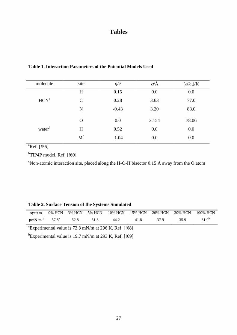
Table 1. Interaction Parameters of the Potential Models Used

molecule site q/e σ/Å (ε/kB)/K

HCNa

H 0.15 0.0 0.0

C 0.28 3.63 77.0

N -0.43 3.20 88.0

waterb

O 0.0 3.154 78.06

H 0.52 0.0 0.0

Mc -1.04 0.0 0.0

aRef. [!56] bTIP4P model, Ref. [!60] cNon-atomic interaction site, placed along the H-O-H bisector 0.15 Å away from the O atom

Table 2. Surface Tension of the Systems Simulated

system 0% HCN 3% HCN 5% HCN 10% HCN 15% HCN 20% HCN 30% HCN 100% HCN

γγγγ/mN m-1 57.8a 52.8 51.3 44.2 41.8 37.9 35.9 31.0b

aExperimental value is 72.3 mN/m at 296 K, Ref. [!68] bExperimental value is 19.7 mN/m at 293 K, Ref. [!69]

28

Table 3. Calculated Properties of the First Three Subsurface Molecular Layers of the

Systems Simulated

subsurface layer

system δ/Å Xc/Å ξ a/Å τ/ps

water HCN

first layer

0% HCN 3.66 22.08 1.09 2.12 29.4

3% HCN 3.91 22.66 1.22 2.31 26.20 200.1

5% HCN 4.03 23.11 1.27 2.36 21.24 167.2

10% HCN 4.41 24.23 1.35 2.55 13.86 77.67

15% HCN 4.65 25.41 1.34 2.72 10.88 55.80

20% HCN 5.09 26.64 1.35 2.82 9.23 39.26

30% HCN 5.16 29.20 1.41 2.96 8.78 28.81

100% HCN 5.33 47.69 1.34 3.03 22.55

second layer

0% HCN 3.65 18.71 1.00 2.08 2.21

3% HCN 3.80 19.24 1.03 2.16 2.10 7.86

5% HCN 3.86 19.63 1.05 2.20 2.00 6.88

10% HCN 4.09 20.50 1.10 2.33 2.16 4.33

15% HCN 4.29 21.47 1.11 2.48 2.62 3.52

20% HCN 4.69 22.42 1.15 2.61 3.45 4.14

30% HCN 4.86 24.67 1.23 2.74 3.26 3.86

100% HCN 5.23 42.78 1.21 2.90 1.86

third layer

0% HCN 3.73 15.46 1.04 2.10 2.28

3% HCN 3.85 15.94 1.04 2.17 2.28 10.51

5% HCN 3.90 16.29 1.05 2.21 2.22 8.21

10% HCN 4.09 17.05 1.07 2.32 2.15 5.76

15% HCN 4.26 17.90 1.06 2.45 2.12 3.56

20% HCN 4.59 18.68 1.07 2.59 2.24 3.74

30% HCN 4.73 20.58 1.14 2.71 2.78 3.48

100% HCN 5.21 37.97 1.16 2.94 1.82

29

Figure Legends

Figure 1. Equilibrium snapshot of the 20% HCN system, as taken out from the simulation.

Molecules belonging to the first, second and third subsurface molecular layers as well as to

the bulk liquid phase are marked by red, green, blue and grey colors, respectively. Darker and

lighter shades of the colors correspond to the HCN and water molecules, respectively. The

snapshot only shows the X > 0 Å half of the basic box.

Figure 2. Number density profile of the water (top panel) and HCN (second panel) molecules

as well as mass density of the entire system (third panel) and its surface layer (bottom panel)

along the macroscopic surface normal axis X in the systems containing 0% HCN (full circles),

3% HCN (red solid lines), 10% HCN (dark blue dash-dotted lines), 20% HCN (light blue

dash-dot-dotted lines), 30% HCN (magenta dotted lines), and 100% HCN (open circles). All

profiles shown are symmetrized over the two liquid-vapor interfaces present in the basic

simulation box. The scale on the right of the second panel refers to the concentration

(molarity) of HCN.

Figure 3. Composition (in terms of HCN mole percentage) of the first (red circles), second

(green squares) and third (blue triangles) subsurface molecular layers as well as of the bulk

liquid phase (black solid line) as a function of the composition of the bulk liquid phase in the

systems simulated.

Figure 4. Mass density profile of the entire system (black solid lines) as well as its first (red

filled circles), second (blue open circles) and third (green asterisks) subsurface molecular

layers along the macroscopic surface normal axis X in the systems containing 3% HCN (top

panel), 10% HCN (second panel), 15% HCN (third panel) and 30% HCN (bottom panel). All

profiles shown are symmetrized over the two liquid-vapor interfaces present in the basic

simulation box.

Figure 5. Number density profile of the water (black solid lines) and HCN (red dashed lines)

molecules of the first subsurface molecular layer along the macroscopic surface normal axis X

in the systems containing 3% HCN (top panel), 10% HCN (second panel), 15% HCN (third

panel) and 30% HCN (bottom panel). The scales on the left and right of the panels refer to the

30

water and HCN densities, respectively. All profiles shown are symmetrized over the two

liquid-vapor interfaces present in the basic simulation box.

Figure 6. Average normal distance of two surface points as a function of their lateral

distance, as obtained in the systems containing 0% HCN (full circles), 3% HCN (red solid

lines), 5% HCN (light green dashed lines), 10% HCN (dark blue dash-dotted lines), 15%

HCN (dark green short dashed lines), 20% HCN (light blue dash-dot-dotted lines), 30%

HCN (magenta dotted lines), and 100% HCN (open circles). The inset shows the average

normal distance vs. lateral distance data in the first (black symbols), second (red symbols)

and third (blue symbols) subsurface molecular layers of the systems containing 3% HCN

(diamonds) and 30% HCN (squares). The curves fitted to the data according to eq. 4 are

shown by dashed lines.

Figure 7. Distribution of the Voronoi polygon area of the molecules in the surface layer, as

calculated regarding all surface molecules (top panel), only the HCN molecules of the surface

layer (middle panel) and only the water molecules of the surface layer (bottom panel) in the

systems containing 0% HCN (full circles), 3% HCN (red solid lines), 5% HCN (green dashed

lines), 10% HCN (dark blue dash-dotted lines), 20% HCN (light blue dash-dot-dotted lines),

30% HCN (magenta dotted lines), and 100% HCN (open circles). In the calculation the

molecules have been represented by their centers projected to the macroscopic plane of the

surface (see the text). To emphasize the exponential decay of the curves the data are shown on

a logarithmic scale.

Figure 8. Instantaneous snapshot of the surface layer of the systems containing 5% HCN (left

panel), 15% HCN (middle panel) and 30% HCN, shown from top view the centers of the

molecules being projected to the macroscopic plane of the surface, YZ. Water and HCN

molecules are represented by red and green balls, respectively.

Figure 9. Survival probability of the water (top panel) and HCN (bottom panel) molecules in

the surface layer of the systems containing 0% HCN (full circles), 3% HCN (red solid lines),

5% HCN (light green dashed lines), 10% HCN (dark blue dash-dotted lines), 15% HCN (dark

green short dashed lines), 20% HCN (light blue dash-dot-dotted lines), 30% HCN (magenta

dotted lines), and 100% HCN (open circles). To emphasize the exponential decay of the

survival probabilities, the plot shows the data on a logarithmic scale.

31

Figure 10. (a) Definition of the local Cartesian frame fixed to the individual surface water

molecules (see the test) and the angles ϑ and φ (right), and γ (left), describing the surface

orientation of the water and HCN molecules, respectively. O, H, C and N atoms are shown by

red, white, grey and blue colors, respectively. (b) Illustration of the division of the surface

layer into three separate zones, marked by A, B and C (see the text).

Figure 11. Orientational maps of the surface water molecules in the systems containing 0%

HCN (top row), 3% HCN (second row), 10% HCN (third row), 15% HCN (fourth row), and

30% HCN (bottom row). The first column corresponds to the entire surface layer, whereas the

second, third and fourth columns to its separate zones C, B, and A, respectively. Lighter

shades of grey indicate higher probabilities. The preferred water orientations corresponding to

the different peaks of the P(cosϑ,φ) orientational maps are also indicated.

Figure 12. Cosine distribution of the angle γ, formed by the vector pointing from the H to the

N atom of the surface HCN molecules and the macroscopic surface normal vector, X,

pointing from the liquid to the vapor phase, in the systems containing 3% HCN (red solid

lines), 10% HCN (blue dash-dotted lines), 15% HCN (green short dashed lines), 30% HCN

(magenta dotted lines), and 100% HCN (open circles). The top panel corresponds to the entire

surface layer, whereas the second, third and fourth panels to its separate zones C, B, and A,

respectively.

Figure 13. Cosine distribution of the angle α, formed by the vectors pointing from the H to

the N atom of two neighboring surface HCN molecules, as obtained in the systems containing

3% HCN (red solid lines), 10% HCN (dark blue dash-dotted lines), 20% HCN (light blue

dash-dot-dotted lines), 30% HCN (magenta dotted lines), and 100% HCN (open circles).

Figure 14. Illustration of the observed orientational preferences of the surface molecules

relative to the macroscopic surface normal as well as to each other. The O, H, C and N atoms

of the water and HCN molecules are shown by red, white, grey and blue colors, respectively.

32

Figure 1.

Fábián et al.

33

Figure 2.

Fábián et al.

0 10 20 30 40 50 600.0

0.2

0.4

0.6

0.00

0.25

0.50

0.75

1.000.000

0.005

0.010

0.015

0.0000.0050.0100.0150.0200.0250.0300.0350.040

0

10

20

30

surface layermass density

ρsu

rf / g cm

-3

X / Å

0% HCN 3% HCN 10% HCN 20% HCN 30% HCN 100% HCN

totalmass density

ρ /

g cm-3

HCNnumberdensity

ρ HC

N /

Å-3

waternumber density

ρ wat /

Å-3

c HC

N/m

ol dm

-3

34

Figure 3.

Fábián et al.

0 5 10 15 20 25 300

20

40

60

80

100

HC

N m

ole

% i

n th

e su

rfac

e la

yers

HCN mole % in the bulk liquid phase

bulk liquid phase first layer second layer third layer

35

Figure 4.

Fábián et al.

0 10 20 30 40 500.0

0.3

0.6

0.90.0

0.3

0.6

0.90.0

0.3

0.6

0.90.0

0.3

0.6

0.9

30% HCN

X / Å

first layer second layer third layer entire system

15% HCN

ρ /

g cm-3

10% HCN

3% HCN

36

Figure 5.

Fábián et al.

20 30 400.000

0.001

0.002

0.000

0.003

0.006

0.000

0.005

0.010

0.00

0.01

0.02

0.000

0.005

0.010

0.000

0.003

0.006

0.0090.000

0.003

0.006

0.000

0.001

0.002

0.003

30% HCN

X / Å

water HCN

surf

surf

15% HCN

ρw

at /Å

-3

10% HCN

3% HCN

ρ

HC

N /Å

-3

37

Figure 6.

Fábián et al.

0 5 10 15 20 250.0

0.5

1.0

1.5

2.0

2.5

3.0

0 5 10 15 20 250

1

2

3

d / Å

l / Å

0% HCN 3% HCN

5% HCN 10% HCN

15% HCN 20% HCN 30% HCN 100% HCN

3% HCN

30% HCN

3% HCN, 1st layer 30% HCN, 1st layer

3% HCN, 2nd layer 30% HCN, 2nd layer

3% HCN, 3rd layer 30% HCN, 3rd layer

d / Å

l / Å

38

Figure 7.

Fábián et al.

0 50 100 150 200

1E-4

1E-3

0.01

0.1

1

1E-4

1E-3

0.01

0.1

1

1E-4

1E-3

0.01

0.1

1

water molecules

A / Å2

HCNmolecules

all molecules 0% HCN 3% HCN 5% HCN 10% HCN 20% HCN 30% HCN 100% HCN

P

(A)

39

40

Figure 8.

Fábián et al.

5% HCN system 15% HCN system 30% HCN system

41

Figure 9.

Fábián et al.

0 20 40 600.1

1

0.01

0.1

1

L(t)

HCN

t/ps

0% HCN 3% HCN 5% HCN 10% HCN 15% HCN 20% HCN 30% HCN 100% HCN

water

42

Figure 10.

Fábián et al.

X

γγγγ

X z

y

x

ϑϑϑϑ

φφφφ (a)

(b)

vapor phaseliquid phase

zone B

zone C zone A

ρmax

/2ρmax

/2

ρmax

ρ

X

43

Figure 11.

Fábián et al.

-1.0 -0.5 0.0 0.5 1.00

30

60

90

-1.0 -0.5 0.0 0.5 1.00

30

60

90

-1.0 -0.5 0.0 0.5 1.00

30

60

90

-1.0 -0.5 0.0 0.5 1.00

30

60

90

-1.0 -0.5 0.0 0.5 1.00

30

60

90

-1.0 -0.5 0.0 0.5 1.00

30

60

90

-1.0 -0.5 0.0 0.5 1.00

30

60

90

-1.0 -0.5 0.0 0.5 1.00

30

60

90

-1.0 -0.5 0.0 0.5 1.00

30

60

90

-1.0 -0.5 0.0 0.5 1.00

30

60

90

-1.0 -0.5 0.0 0.5 1.00

30

60

90

-1.0 -0.5 0.0 0.5 1.00

30

60

90

-1.0 -0.5 0.0 0.5 1.00

30

60

90

-1.0 -0.5 0.0 0.5 1.00

30

60

90

-1.0 -0.5 0.0 0.5 1.00

30

60

90

-1.0 -0.5 0.0 0.5 1.00

30

60

90

-1.0 -0.5 0.0 0.5 1.00

30

60

90

-1.0 -0.5 0.0 0.5 1.00

30

60

90

-1.0 -0.5 0.0 0.5 1.00

30

60

90

-1.0 -0.5 0.0 0.5 1.00

30

60

90

I

φ/de

g

φ/de

g

φ/de

g

φ/de

g

cosϑ

IC

III

cosϑcosϑ

I

IA

II

cosϑ

cosϑ

I

I

I

cosϑcosϑcosϑcosϑ

cosϑ cosϑ cosϑ cosϑ

cosϑcosϑcosϑcosϑ

cosϑ cosϑ cosϑ

30% HCN

15% HCN

10% HCN

3% HCN

0% HCN

entiresurface layer

region Aregion Bregion C

I

φ/de

g

φ/de

gφ/

deg

φ/de

g

φ/de

g

φ/de

g

I

IC

I

φ/de

g

φ/de

g

φ/de

g

φ/de

gφ/

deg

φ/de

g

φ/de

g

φ/de

gφ/

deg

φ/de

g

IA

I

IC

I

IA

I

IC

I

IA

44

Figure 12.

Fábián et al.

-1.0 -0.5 0.0 0.5 1.0

0.01

0.02

0.03

0.01

0.02

0.03

0.01

0.02

0.03

0.01

0.02

0.03

0.04

region C

P(c

osγ)

cosγ

3% HCN 10% HCN 15% HCN 30% HCN 100% HCN

region B

region A

entire surface layer

45

Figure 13.

Fábián et al.

-1.00 -0.75 -0.50 -0.25 0.00 0.25 0.50 0.75 1.00

0.020

0.025

0.030

0.035

0.040

P(c

osα)

cosα

3% HCN 10% HCN 20% HCN 30% HCN 100% HCN

46

Figure 14.

Fábián et al.

47

Table of Contents Graphics: