Embed Size (px)
Citation preview
FLINDERS AND GILBERT AGRICUTURAL RESOURCE ASSESSMENT
Irrigation costs and benefits A technical report to the Australian Government from the CSIRO Flinders and Gilbert Agricultural Resource Assessment, part of the North Queensland Irrigated Agriculture Strategy
Lisa Brennan McKellar1, Marta Monjardino2, Rosalind Bark1, Glyn Wittwer3, Onil Banerjee1#, Andrew Higgins1, Neil MacLeod1, Neville Crossman2, Di Prestwidge1 and Luis Laredo1 1CSIRO Ecosystem Sciences, Brisbane
# now with Inter-American Development Bank, Washington.
2CSIRO Ecosystem Sciences, Adelaide
3Centre for Policy Studies, Monash University, Melbourne.
December 2013
Water for a Healthy Country Flagship Report series ISSN: 1835-095X
Australia is founding its future on science and innovation. Its national science agency, CSIRO, is a powerhouse of ideas, technologies and skills.
CSIRO initiated the National Research Flagships to address Australia’s major research challenges and opportunities. They apply large scale, long term, multidisciplinary science and aim for widespread adoption of solutions. The Flagship Collaboration Fund supports the best and brightest researchers to address these complex challenges through partnerships between CSIRO, universities, research agencies and industry.
Consistent with Australia’s national interest, the Water for a Healthy Country Flagship aims to develop science and technologies that improve the social, economic and environmental outcomes from water, and deliver $3 billion per year in net benefits for Australia by 2030. The Sustainable Agriculture Flagship aims to secure Australian agriculture and forest industries by increasing productivity by 50 percent and reducing carbon emissions intensity by at least 50 percent by 2030.
For more information about Water for a Healthy Country Flagship, Sustainable Agriculture Flagship or the National Research Flagship Initiative visit <http://www.csiro.au/flagships>.
Citation
Brennan McKellar L, Monjardino M, Bark R , Wittwer G, Banerjee O, Higgins A, MacLeod N, Crossman N, Prestwidge D and Laredo L (2013) Irrigation costs and benefits. A technical report to the Australian Government from the CSIRO Flinders and Gilbert Agricultural Resource Assessment, part of the North Queensland Irrigated Agriculture Strategy. CSIRO Water for a Healthy Country and Sustainable Agriculture flagships, Australia.
Copyright
© Commonwealth Scientific and Industrial Research Organisation 2013. To the extent permitted by law, all rights are reserved and no part of this publication covered by copyright may be reproduced or copied in any form or by any means except with the written permission of CSIRO.
Important disclaimer
CSIRO advises that the information contained in this publication comprises general statements based on scientific research. The reader is advised and needs to be aware that such information may be incomplete or unable to be used in any specific situation. No reliance or actions must therefore be made on that information without seeking prior expert professional, scientific and technical advice. To the extent permitted by law, CSIRO (including its employees and consultants) excludes all liability to any person for any consequences, including but not limited to all losses, damages, costs, expenses and any other compensation, arising directly or indirectly from using this publication (in part or in whole) and any information or material contained in it.
Flinders and Gilbert Agricultural Resource Assessment acknowledgments
This report was prepared for the Office of Northern Australia in the Australian Government Department of Infrastructure and Regional Development under the North Queensland Irrigated Agriculture Strategy <http://www.regional.gov.au/regional/ona/nqis.aspx>. The Strategy is a collaborative initiative between the Office of Northern Australia, the Queensland Government and CSIRO. One part of the Strategy is the Flinders and Gilbert Agricultural Resource Assessment, which was led by CSIRO. Important aspects of the Assessment were undertaken by the Queensland Government and TropWATER (James Cook University).
The Strategy was guided by two committees:
(i) the Program Governance Committee, which included the individuals David Crombie (GRM International), Scott Spencer (SunWater, during the first part of the Strategy) and Paul Woodhouse (Regional Development Australia) as well as representatives from the following organisations: Australian Government Department of Infrastructure and Regional Development; CSIRO; and the Queensland Government.
(ii) the Program Steering Committee, which included the individual Jack Lake (Independent Expert) as well as representatives from the following organisations: Australian Government Department of Infrastructure and Regional Development; CSIRO; the Etheridge, Flinders and McKinlay shire councils; Gulf Savannah Development; Mount Isa to Townsville Economic Development Zone; and the Queensland Government.
This report was reviewed by Professor John Rolfe, R & Z Consulting and Central Queensland University, and David Pearce, Executive Director, The Centre for International Economics.
In addition to the reviewers who provided advice that improved the quality of our report, the authors acknowledge the many people who provided a great deal of help in the preparation of this report. We are particularly indebted to the local community of the Flinders and Gilbert catchments, particularly those who contributed their time to formal surveys of their attitudes to agricultural development in the two catchments. Julie Harrison, the FRAP Project Officer, provided an enormous amount of assistance to the team. Local government staff in both catchments freely assisted with our many enquiries. We are grateful for information provided by State Government staff: Steph Hogan for information and advice on water planning and regulation, and Greg Mason also helped us make contact with landholders and provided access to information. We also thank Fred Chudleigh, Andrew Zull, and Mark Poggio for assisting with information. Colleagues in CSIRO and elsewhere provided freely of their time and expertise to help with the Assessment. This was often at short notice. The list is long, but we’d particularly like to thank Andrew Ash, Chris Stokes, Robyn Cowley, Cam McDonald, Lindsay Bell, Leigh Hunt, Stuart Whitten, Di Mayberry, Kaitlyn Stutz and Steve Yeates.
Director’s foreword | i
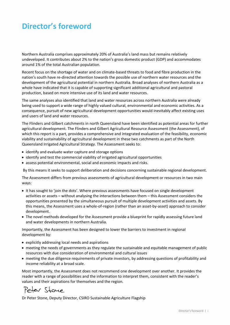
Director’s foreword
Northern Australia comprises approximately 20% of Australia’s land mass but remains relatively undeveloped. It contributes about 2% to the nation’s gross domestic product (GDP) and accommodates around 1% of the total Australian population.
Recent focus on the shortage of water and on climate-based threats to food and fibre production in the nation’s south have re-directed attention towards the possible use of northern water resources and the development of the agricultural potential in northern Australia. Broad analyses of northern Australia as a whole have indicated that it is capable of supporting significant additional agricultural and pastoral production, based on more intensive use of its land and water resources.
The same analyses also identified that land and water resources across northern Australia were already being used to support a wide range of highly valued cultural, environmental and economic activities. As a consequence, pursuit of new agricultural development opportunities would inevitably affect existing uses and users of land and water resources.
The Flinders and Gilbert catchments in north Queensland have been identified as potential areas for further agricultural development. The Flinders and Gilbert Agricultural Resource Assessment (the Assessment), of which this report is a part, provides a comprehensive and integrated evaluation of the feasibility, economic viability and sustainability of agricultural development in these two catchments as part of the North Queensland Irrigated Agricultural Strategy. The Assessment seeks to:
• identify and evaluate water capture and storage options • identify and test the commercial viability of irrigated agricultural opportunities • assess potential environmental, social and economic impacts and risks.
By this means it seeks to support deliberation and decisions concerning sustainable regional development.
The Assessment differs from previous assessments of agricultural development or resources in two main ways:
• It has sought to ‘join the dots’. Where previous assessments have focused on single development activities or assets – without analysing the interactions between them – this Assessment considers the opportunities presented by the simultaneous pursuit of multiple development activities and assets. By this means, the Assessment uses a whole-of-region (rather than an asset-by-asset) approach to consider development.
• The novel methods developed for the Assessment provide a blueprint for rapidly assessing future land and water developments in northern Australia.
Importantly, the Assessment has been designed to lower the barriers to investment in regional development by:
• explicitly addressing local needs and aspirations • meeting the needs of governments as they regulate the sustainable and equitable management of public
resources with due consideration of environmental and cultural issues • meeting the due diligence requirements of private investors, by addressing questions of profitability and
income reliability at a broad scale.
Most importantly, the Assessment does not recommend one development over another. It provides the reader with a range of possibilities and the information to interpret them, consistent with the reader’s values and their aspirations for themselves and the region.
Dr Peter Stone, Deputy Director, CSIRO Sustainable Agriculture Flagship
ii |Irrigation costs and benefits
The Flinders and Gilbert Agricultural Resource Assessment team
Project Director Peter Stone
Project Leaders Cuan Petheram, Ian Watson
Reporting Team Heinz Buettikofer, Becky Schmidt, Maryam Ahmad, Simon Gallant, Frances Marston, Greg Rinder, Audrey Wallbrink
Project Support Ruth Palmer, Daniel Aramini, Michael Kehoe, Scott Podger
Communications Leane Regan, Claire Bobinskas, Dianne Flett2, Rebecca Jennings
Data Management Mick Hartcher
Activities
Agricultural productivity Tony Webster, Brett Cocks, Jo Gentle6, Dean Jones, Di Mayberry, Perry Poulton, Stephen Yeates, Ainsleigh Wixon
Aquatic and riparian ecology Damien Burrows1, Jon Brodie1, Barry Butler1, Cassandra James1, Colette Thomas1, Nathan Waltham1
Climate Cuan Petheram, Ang Yang
Instream waterholes David McJannet, Anne Henderson, Jim Wallace1
Flood mapping Dushmanta Dutta, Fazlul Karim, Steve Marvanek, Cate Ticehurst
Geophysics Tim Munday, Tania Abdat, Kevin Cahill, Aaron Davis
Groundwater Ian Jolly, Andrew Taylor, Phil Davies, Glenn Harrington, John Knight, David Rassam
Indigenous water values Marcus Barber, Fenella Atkinson5, Michele Bird2, Susan McIntyre-Tamwoy5
Water storage Cuan Petheram, Geoff Eades2, John Gallant, Paul Harding3, Ahrim Lee3, Sylvia Ng3, Arthur Read, Lee Rogers, Brad Sherman, Kerrie Tomkins, Sanne Voogt3
Irrigation infrastructure John Hornbuckle
Land suitability Rebecca Bartley, Daniel Brough3, Charlie Chen, David Clifford, Angela Esterberg3, Neil Enderlin3, Lauren Eyres3, Mark Glover, Linda Gregory, Mike Grundy, Ben Harms3, Warren Hicks, Joseph Kemei, Jeremy Manders3, Keith Moody3, Dave Morrison3, Seonaid Philip, Bernie Powell3, Liz Stower, Mark Sugars3, Mark Thomas, Seija Tuomi, Reanna Willis3, Peter R Wilson2
River modelling Linda Holz, Julien Lerat, Chas Egan3, Matthew Gooda3, Justin Hughes, Shaun Kim, Alex Loy3, Jean-Michel Perraud, Geoff Podger
The Flinders and Gilbert Agricultural Resource Assessment team | iii
Socio-economics Lisa Brennan McKellar, Neville Crossman, Onil Banerjee, Rosalind Bark, Andrew Higgins, Luis Laredo, Neil MacLeod, Marta Monjardino, Carmel Pollino, Di Prestwidge, Stuart Whitten, Glyn Wittwer4
Note: all contributors are affiliated with CSIRO unless indicated otherwise. Activity Leaders are underlined. 1 TropWATER, James Cook University, 2 Independent consultant, 3 Queensland Government, 4 Monash University, 5 Archaeological Heritage Management Solutions, 6University of Western Sydney
iv |Irrigation costs and benefits
Shortened forms
AEM airborne electromagnetics
AHD Australian Height Datum
APSIM Agricultural Production Systems Simulator
AWRC Australian Water Resources Council
CGE Computable General Equilibrium
CSIRO Commonwealth Scientific and Industrial Research Organisation
DEM digital elevation model
GCMs global climate models
GCM-ES global climate model output empirically scaled to provide catchment-scale variables
IPCC AR4 the Fourth Assessment Report of the Intergovernmental Panel on Climate Change
IQQM Integrated Quantity-Quality Model – a river systems model
Landsat TM Landsat Thematic Mapper
MODIS Moderate Resolution Imaging Spectroradiometer
NQIAS North Queensland Irrigated Agriculture Strategy
NRM natural resource management
ONA the Australian Government Office of Northern Australia
OWL the Open Water Likelihood algorithm
PAWC plant available water capacity
PE potential evaporation
RCP representative concentration pathway
Sacramento a rainfall-runoff model
SALI the Soil and Land Information System for Queensland
SLAs statistical local areas
SRTM shuttle radar topography mission
TRaCK Tropical Rivers and Coastal Knowledge Research Hub
WRON CSIRO’s Water Resource Observation Network
Units | v
Units
MEASUREMENT UNITS DESCRIPTION
GL gigalitres, 1,000,000,000 litres
keV kilo-electronvolts
kL kilolitres, 1000 litres
km kilometres, 1000 metres
L litres
m metres
mAHD metres above Australian Height Datum
MeV mega-electronvolts
mg milligrams
ML megalitres, 1,000,000 litres
vi |Irrigation costs and benefits
Preface
The Flinders and Gilbert Agricultural Resource Assessment (the Assessment) aims to provide information so that people can answer questions such as the following in the context of their particular circumstances in the Flinders and Gilbert catchments:
• What soil and water resources are available for irrigated agriculture? • What are the existing ecological systems, industries, infrastructure and values? • What are the opportunities for irrigation? • Is irrigated agriculture economically viable? • How can the sustainability of irrigated agriculture be maximised?
The questions – and the responses to the questions – are highly interdependent and, consequently, so is the research undertaken through this Assessment. While each report may be read as a stand-alone document, the suite of reports must be read as a whole if they are to reliably inform discussion and decision making on regional development.
The Assessment is producing a series of reports:
• Technical reports present scientific work at a level of detail sufficient for technical and scientific experts to reproduce the work. Each of the 12 research activities (outlined below) has a corresponding technical report.
• Each of the two catchment reports (one for each catchment) synthesises key material from the technical reports, providing well-informed but non-scientific readers with the information required to make decisions about the opportunities, costs and benefits associated with irrigated agriculture.
• Two overview reports – one for each catchment – are provided for a general public audience. • A factsheet provides key findings for both the Flinders and Gilbert catchments for a general public
audience.
All of these reports are available online at <http://www.csiro.au/FGARA>. The website provides readers with a communications suite including factsheets, multimedia content, FAQs, reports and links to other related sites, particularly about other research in northern Australia.
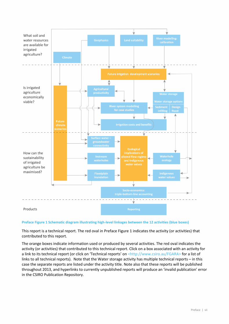
The Assessment is divided into 12 scientific activities, each contributing to a cohesive picture of regional development opportunities, costs and benefits. Preface Figure 1 illustrates the high-level linkages between the 12 activities and the general flow of information in the Assessment. Clicking on an ‘activity box’ links to the relevant technical report.
The Assessment is designed to inform consideration of development, not to enable particular development activities. As such, the Assessment informs – but does not seek to replace – existing planning processes. Importantly, the Assessment does not assume a given regulatory environment. As regulations can change, this will enable the results to be applied to the widest range of uses for the longest possible time frame. Similarly, the Assessment does not assume a static future, but evaluates three distinct scenarios:
• Scenario A – historical climate and current development • Scenario B – historical climate and future irrigation development • Scenario C – future climate and current development.
As the primary interest was in evaluating the scale of the opportunity for irrigated agriculture development under the current climate, the future climate scenario (Scenario C) was secondary in importance to scenarios A and B. This balance is reflected in the allocation of resources throughout the Assessment.
The approaches and techniques used in the Assessment have been designed to enable application elsewhere in northern Australia.
Preface | vii
Preface Figure 1 Schematic diagram illustrating high-level linkages between the 12 activities (blue boxes)
This report is a technical report. The red oval in Preface Figure 1 indicates the activity (or activities) that contributed to this report.
The orange boxes indicate information used or produced by several activities. The red oval indicates the activity (or activities) that contributed to this technical report. Click on a box associated with an activity for a link to its technical report (or click on ‘Technical reports’ on <http://www.csiro.au/FGARA> for a list of links to all technical reports). Note that the Water storage activity has multiple technical reports – in this case the separate reports are listed under the activity title. Note also that these reports will be published throughout 2013, and hyperlinks to currently unpublished reports will produce an ‘invalid publication’ error in the CSIRO Publication Repository.
viii |Irrigation costs and benefits
Executive summary
The economic viability of potential irrigated agriculture development in the Flinders and Gilbert Catchments was considered at a range of scales. This report presents a set of analyses which presents:
• costs and benefits of incorporating irrigated fodder crops into existing beef production systems, • costs and benefits of developing land for irrigated cropping, at both scheme scale and farm scale, • regional and national benefits of investment in irrigated agriculture, taking into account not just
irrigated agriculture per se, but the associated economic activity that accompanies such development (e.g. construction activity and processing industries),
• a review of the numerous legislation and regulations pertaining to land management and potential irrigation development,
• supply chain analyses to estimate transport costs savings that could be achieved if new processing facilities (abattoir, cotton gin, sugar mill) were built locally to service new irrigated agriculture.
The main findings are:
Overall
• An analysis of incorporating irrigated forages into representative beef operations in the Flinders and Gilbert catchments suggest that the increased revenues from cattle production are not sufficient to offset the costs which include capital costs of on-farm dams and irrigation infrastructure.
• An analysis of the net benefits of investing in irrigation to undertake cropping also shows that capital costs of irrigation development impact substantially on investment performance, and that crop gross margins may need to be sustained reliably and at high levels to offset costs. There are, however, profitable opportunities.
• A generic scheme-scale analysis explored the whole-of-development financial performance under a range of scheme-scale capital costs and sizes of irrigation developments. Irrigators could not afford to pay a price to fully cover scheme capital and operating costs, expect under a limited set of circumstances (of low capital costs and high gross margins).
• A large set of Acts of legislation are applicable to irrigation development – the implication for irrigation development should be assessed on a case by case basis.
• A regional-scale analysis of implementing several irrigation developments and associated processing facilities in the Flinders and Gilbert catchments shows the potential for the enlargement of the regional economy of North-West Queensland, but a negative economic impact for the nation.
• Building a new abattoir in Cloncurry and a new cotton gin in Carters Towers can result in substantial transport cost savings to Flinders beef producers and cotton growers. Sugarcane growers in the Gilbert (serviced by a dam in Dagworth) could benefit from reduced transport costs from a sugar mill in Palmers Hut, but the trade-off is the 100+km distance from Georgetown.
Farm-scale analyses
• The capital costs of irrigation development, particularly when on-farm dam is included, are high and impact substantially on investment performance.
• Gross margins can vary considerably from year to year, and with large capital investments, they need to be sustained at high levels for the investment to be viable.
Executive summary | ix
• Water reliability is a significant issue. Profitable investments under reliable allocation delivery can become unviable with reduced water reliability.
• Timing matters – poor crop yield outcomes early in the life of the investment will further disadvantage the investment performance.
• The benefits from irrigation to beef cattle production is by means of overcoming seasonal feed shortages. Notably, the main economic value of irrigation accrues from:
o Higher turnoff weight attracting a higher price per head in the market achieved through a combination of longer fattening period and higher daily live weight gains;
o Reduced need for costly supplementary feed, such as grain and purchased hay, during the dry season due to provision of on-farm valuable feed;
o Sale of hay as a complementary source of revenue; • Investing in irrigation to incorporate irrigated forages into the typical beef operations of the gulf
catchments of north Queensland appears to be economically unattractive because the capital costs of irrigation far outweigh the returns from raising the productivity of the cattle herd.
Regional-scale analyses
• The net benefits of development of irrigated agriculture in North West Queensland were determined using TERM, a dynamic multi-regional computable general equilibrium (CGE) model of Australia.
• The irrigation development modelled was the full set of case studies presented in Chapters 8-10. All case studies were modelled as if they were implemented simultaneously, and does not account for case study developments that are mutually exclusive.
• Assuming that the current economic environment prevails until 2027, the model predicted that the economy of North-West Queensland will enlarge, notably with an initial boost to employment, however the long-term impact, over the duration of this period, is predicted to be relatively small.
• At the national scale of impact, the short-term economic boosts during the irrigation investment phase, while providing local and national stimulus, are not sufficient to justify investment expenditures, and over the full duration of project the returns do not outweigh costs. As a result, the net present value of benefits is negative. The annualised net present value of the welfare impact is minus $69 million.
Supply chain analyses
• Locating a new abattoir in Cloncurry results in an average transport cost of $27/head, a saving of $34/head. If a Cloncurry abattoir slaughters 100,000 head of cattle a year, there would be a collective transport cost saving of $3.26 million/year. If it slaughtered 150,000 head/year, there would be a transport cost saving of $5.1 million/year. This does not include additional benefits in terms of improved animal condition upon arrival at the abattoir, and reduced green house gas emissions.
• Building a sugar mill in Georgetown to process sugarcane grown on properties supplied by the Dagworth dam would result in transport costs much higher than any other sugar mill in Australia. However, sealing roads to the Dagworth area would reduce the costs of cane transport to the mill by about 20% (average of $16/t). If the sugar mill was to process an average of 2 million tonnes of cane per year, this would reduce transport costs by $8 million. Locating a sugar mill in Palmer Hut near the Dagworth area would reduce the average transport cost to the mill to about $2.80/t. However, this would increase the cost of transporting sugar to Townsville port from $41.7/t to $65/t, giving a total transport cost per tonne of cane (unprocessed equivalent) of $12.6/t. This is about half the cost of the base case of a mill at Georgetown.
• Building a cotton gin in Charters Towers would reduce the transport distance from properties near Richmond and Hughenden to the Gin by an average of 480km, but increase the transport distance from the gin to Brisbane by that same amount. The main benefit is a larger portion of the total

x |Irrigation costs and benefits
travel will be processed cotton without the cottonseed and trash. This scenario would reduce the total transport cost to an average of $418/t (unprocessed crop equivalent).
Contents | xi
Contents
Director’s foreword ............................................................................................................................................. i
The Flinders and Gilbert Agricultural Resource Assessment team .................................................................... ii
Shortened forms ................................................................................................................................................ iv
Units ............................................................................................................................................................... v
Executive summary............................................................................................................................................ vi
Overall ................................................................................................................................................ viii
Farm-scale analyses ........................................................................................................................... viii
Regional-scale analyses ........................................................................................................................ ix
Supply chain analyses ........................................................................................................................... ix
1 Introduction 1
1.1 Purpose of this report ................................................................................................................. 1
1.2 Brief description of study regions ............................................................................................... 1
1.3 Structure of this report ............................................................................................................... 1
2 Farm-scale and scheme-scale financial evaluation for irrigated cropping developments 3
2.1 Introduction ................................................................................................................................ 3
2.2 Discounted cash flow analysis framework .................................................................................. 3
2.3 Investment performance for farm-scale irrigation developments ........................................... 11
2.4 Investment performance for scheme-scale irrigation developments ...................................... 18
2.5 Conclusion ................................................................................................................................. 25
3 Farm-scale evaluation of irrigated fodder production 26
3.1 Introduction .............................................................................................................................. 26
3.2 Methods .................................................................................................................................... 26
3.3 Results ....................................................................................................................................... 41
3.4 Discussion ................................................................................................................................. 54
3.5 Conclusion ................................................................................................................................. 54
4 Legislation and regulation 55
4.1 Introduction .............................................................................................................................. 55
4.2 Legislation and regulation ......................................................................................................... 56
5 Analysis of irrigated agricultural development options in northern Australia 65
5.1 Introduction .............................................................................................................................. 65
5.2 Regional Profile ......................................................................................................................... 65
5.3 Methods .................................................................................................................................... 66
5.4 Case study design ...................................................................................................................... 68
xii |Irrigation costs and benefits
5.5 Results ....................................................................................................................................... 73
5.6 Conclusions ............................................................................................................................... 80
6 Evaluating the logistics costs from new or modified supply chains 81
6.1 Introduction .............................................................................................................................. 81
6.2 Objectives and scope ................................................................................................................ 81
6.3 Outline of Transport Model and Assumptions ......................................................................... 82
6.4 Cattle ......................................................................................................................................... 83
6.5 Sugar ......................................................................................................................................... 86
6.6 Cotton ....................................................................................................................................... 88
7 Conclusion 89
8 References 90
Contents | xiii
Figures Figure 1.1 Map of the northern Queensland gulf catchments, including Georgetown in the Gilbert catchment and Richmond in the Flinders catchment ........................................................................................ 2
Figure 2.1 Annual world indicator prices of selected commodities ................................................................. 10
Figure 2.2 Indexes of prices received by farmers in Australia .......................................................................... 11
Figure 2.3. Financial performance indicators for selected irrigation investment scenarios with storages ranging from 952ML to 3,810ML capacity under a $1500 crop gross margin and a 5% and 7% discount rate. At the 7% discount rate, the impact of a staged investment implementation and assumption of no asset residual value is also presented. ............................................................................................................. 16
Figure 3.1 Growth patterns of beef cattle in northern Australia. .................................................................... 29
Figure 3.2 Structure of the North Australia Beef System Analyser (NABSA) bio-economic simulation model ................................................................................................................................................................ 31
Figure 3.3 Flow-chart representation of the cattle herd structure underlying the baseline scenario for a Georgetown breeding operation ...................................................................................................................... 33
Figure 3.4 Flow-chart representation of the cattle herd structure underlying the baseline scenario for a Richmond fattening operation ......................................................................................................................... 34
Figure 3.5 Change in annual net profit between 1996 and 2010 for the five Georgetown scenarios ............. 42
Figure 3.6 Change in annual net profit for a standard, high and low cost of pumping water over the selected 15-year period of 1996-2010 for Scenario 4 (500 ha lablab for hay) in Georgetown ....................... 43
Figure 3.7 Change in annual net profit for a standard, high and low purchase price of urea fertiliser over the selected 15-year period of 1996-2010 for Scenario 5 (1000 ha sorghum for hay) in Georgetown. ......... 43
Figure 3.8 Cumulative distribution functions (CDFs) for the net value of irrigation of the four irrigation scenarios in Georgetown .................................................................................................................................. 44
Figure 3.9 Change in annual net profit between 1996 and 2010 for the five Richmond scenarios ................. 47
Figure 3.10 Change in annual net profit for a standard, high and low sale price of live weight animals over the selected 15-year period of 1996-2010 for Scenario 2 (200 ha bambatsi panic for grazing) in Richmond .......................................................................................................................................................... 48
Figure 3.11 Change in annual net profit for a standard, high and low sale price of hay over the selected 15-year period of 1996-2010 for Scenario 5 (1000 ha sorghum for hay) in Richmond ................................... 48
Figure 3.12 Cumulative distribution functions (CDFs) for the net value of irrigation of the four irrigation scenarios in Richmond ...................................................................................................................................... 49
Figure 3.13 Change in annual net profit for a standard, high and low total efficiency level of irrigation over the selected 15-year period of 1996-2010 for Scenario 3 (200 ha bambatsi panic for grazing), using minimum storage size, in Richmond ................................................................................................................ 52
Figure 3.14 Cumulative distribution functions (CDFs) for a standard, high and low levels of reliability of water supply for the 107 streams of 15 years over the period of 1890 to 2010 for Scenario 3 (200 ha bambatsi panic for grazing), using minimum storage size, in Richmond. ........................................................ 53
Figure 4.1: Land tenure .................................................................................................................................... 59
Figure 5.1 Aggregate consumption and investment for North West Queensland (per cent deviation from forecast) ............................................................................................................................................................ 74
Figure 5.2 Aggregate consumption and investment for Australia (per cent deviation from forecast) ............ 74
Figure 5.3 Labour market, Queensland’s North West statistical division(per cent deviation from forecast) . 74
xiv |Irrigation costs and benefits
Figure 5.4 Income side components of real GDP in Queensland’s North West statistical division (contribution to per cent deviation from forecast) .......................................................................................... 75
Figure 5.5 Export and import volumes (%), balance of trade % of GDP, Australia (relative to forecast) ........ 76
Figure 5.6 Real exchange rate and terms of trade, Australia (% deviation from forecast) .............................. 76
Figure 5.7 Farm and downstream investment, Queensland’s North West statistical division ($m deviation from forecast) ................................................................................................................................... 79
Figure 5.8 Key outputs, Queensland’s North West statistical division ($m deviation from forecast) ............. 79
Figure 6.1 Simplified view of accessibility of heavy vehicles in Queensland ................................................... 83
Figure 6.2 Current destinations and cattle numbers of top 100 property movements ................................... 84
Figure 6.3 Existing (modelled) transport routes for representative 100 cattle properties. ............................. 85
Figure 6.4 New transport routes for representative 100 cattle properties is supplying to new Cloncurry abattoir. ............................................................................................................................................................ 85
Figure 6.5 Transport paths to Georgetown for 5 representative locations of sugar in Dagworth and 10 representative locations of cotton in Greenhills. ............................................................................................. 86
Contents | xv
Tables Table 2.1 Sowing date, applied irrigation water, crop yield, irrigation type, price, variable cost and gross margin for crops in the Flinders catchment ....................................................................................................... 7
Table 2.2 Sowing date, applied irrigation water, crop yield, irrigation type, price, variable cost and gross margin for crops in the Gilbert catchment. ........................................................................................................ 8
Table 2.3 Pumping costs by irrigation type ........................................................................................................ 9
Table 2.4 Sensitivity of cotton gross margin to distance to gin and cotton price based on cotton yield simulated for the Flinders catchment. ............................................................................................................. 10
Table 2.5 Assumptions for analysis of irrigation development investment ..................................................... 12
Table 2.6 Other capital costs of irrigation investment (excluding irrigation storage and conveyance costs) . 13
Table 2.7 Financial performance indicators for selected irrigation investment scenarios with storages ranging from 952ML to 3,810ML capacity under a $1500 crop gross margin and a 5% and 7% discount rate. .................................................................................................................................................................. 15
Table 2.8 Net present values for selected irrigation investment scenarios with storages ranging from 952ML to 3,810ML capacity under crop gross margins ranging from $500 to $2500/ha with a 5% and 7% discount rate. .................................................................................................................................................... 16
Table 2.9 Net present value (NPV) and internal rate of return (IRR) ............................................................... 17
Table 2.10 Capital and operating cost assumptions for different scales of irrigation development ............... 20
Table 2.11 Irrigation development-area-scale capital and operating costs ..................................................... 21
Table 2.12 Break-even annual gross margins required under different combinations of scheme-sale capital cost and irrigated area .......................................................................................................................... 22
Table 2.13 Scaling factors for gross margins accounting for changed reliability (60% to 90%) and timing of failed years (early and late in the cash flow) ............................................................................................... 23
Table 2.14 Minimum price charged by supplier to cover capital and operating costs under different combinations of scheme-sale capital cost and irrigated area. Assumptions include 100% reliability of water allocation and a 7% discount rate. ......................................................................................................... 23
Table 2.15 Minimum price charged by supplier to cover operating costs under infrastructure capital cost and irrigated area combinations. Assumptions include 100% reliability of water allocation and a 7% discount rate. .................................................................................................................................................... 24
Table 2.16 Capacity of irrigators to pay for water (break-even water price) under different combinations of gross margin and irrigation use .................................................................................................................... 24
Table 3.1 Agronomic parameter settings for each forage species in Georgetown .......................................... 32
Table 3.2 Agronomic parameter settings for each forage species in Richmond .............................................. 32
Table 3.3 NPV analysis. Minimum, maximum, mean and median values of net present value (NPV) over the full range of 15-year sequences simulated with the NABSA at the start of each year of the 121-year period through to the last 15-year series (1996-2010) for Georgetown and Richmond baseline (nil-irrigation) case. ................................................................................................................................................. 35
Table 3.4 Scenarios features for Georgetown. Key features of the five scenarios in Georgetown based on the underlying assumptions of forage type water requirements, irrigated area, storage size, irrigation system, feed base, as well as age, weight and price of animals sold ............................................................... 37
Table 3.5 Scenarios features for Richmond. Key features of the five scenarios in Richmond based on the underlying assumptions of forage type water requirements, irrigated area, irrigated system, irrigation efficiencies, storage size, feed base, as well as age, weight and price of animals sold ................................... 38
xvi |Irrigation costs and benefits
Table 3.6 Key parameters for sensitivity analysis. Values of uncertain parameters used in the sensitivity analysis (model default values in bold) for both case studies. ........................................................................ 40
Table 3.7 Key economic parameters for multi-factorial analysis in Georgetown and Richmond. Values of uncertain parameters used in the multi-factorial analysis (model default values in bold) and probability of occurrence for each parameter value .......................................................................................................... 41
Table 3.8 Simulation results under default parameters for Georgetown. Key average model simulation results across the selected 15-year period of 1996 to 2010 for the five Georgetown scenarios using model default parameters ................................................................................................................................ 42
Table 3.9 Summary of changes for Georgetown. Key changes in irrigated area, forage type water requirements, total irrigation efficiency, storage size and total annual fixed costs of irrigation investment required to adjust all scenarios to 200 ha in Georgetown ............................................................................... 45
Table 3.10 Georgetown simulation results for 200 ha irrigation. Key average model simulation results across the selected 15-year period of 1996 to 2010 for the baseline and the four irrigation scenarios adjusted to 200 ha using minimum storage size to meet irrigation demand .................................................. 46
Table 3.11 Simulation results under default parameters in Richmond. Key average model simulation results across the selected 15-year period of 1996 to 2010 for the five Richmond scenarios using model default parameters ........................................................................................................................................... 47
Table 3.12 Summary of changes for Richmond. Key changes in irrigated area, forage type water requirements, total irrigation efficiency, storage size and total annual fixed costs of irrigation investment required to adjust all scenarios to 200 ha in Richmond ................................................................................... 50
Table 3.13 Richmond simulation results for 200 ha of irrigation. Key average model simulation results across the selected period of 1996 to 2010 for the baseline and the four irrigation scenarios adjusted to 200 ha using minimum storage size to meet irrigation demand ..................................................................... 51
Table 3.14 NPV analysis for a range of reliability levels of supply of irrigation water. Values of net present value (NPV) of net profit over the full range of 15-year sequences simulated with the NABSA for the 121-year period in Scenario 3, using minimum storage size, in Richmond ............................................... 52
Table 3.15 Simulated results for three levels of irrigation costs on the scenario with the overall highest net value of irrigation. Key average economic results across the selected 15-year period of 1996 to 2010 for the Richmond scenario with 200 ha of bambatsi panic for grazing using minimum storage size to meet irrigation demand. Results for the baseline scenario are included for reference. ................................. 53
Table 4.1 Additional water licences (to Gulf WRP “general unallocated water”) allocated in 2013 ............... 55
Table 4.2 Summary of Land tenure: descriptions and permits required for irrigated agriculture................... 60
Table 5.1 Population (2008 and projected to 2031) and major employers by shire ....................................... 66
Table 5.2 Sectors and regions in TERM ............................................................................................................ 67
Table 5.3 Irrigation development investment, Cave Hill .................................................................................. 69
Table 5.4 Capital investment and annual operating and maintenance costs, O’Connell Creek ...................... 70
Table 5.5 Capital investment and annual operating and maintenance costs, Copperfield Gorge ................... 71
Table 5.6 Capital investment and annual operating and maintenance costs, Dagworth ................................ 72
Table 5.7 Capital investment and annual operating and maintenance costs, Greenhills ................................ 73
Table 5.8 Estimated value of farm outputs based on case studies ($m 2011 prices, in 2022) ....................... 77
Table 5.9 Endowments and technological change in Queensland’s North West statistical division ($m 2011 prices, in 2022) ........................................................................................................................................ 78
Table 6.1 Road transport costs per vehicle ($/km) .......................................................................................... 82
Table 6.2 Base case transport costs for each sugar location, with unsealed roads to a mill at Georgetown .. 87
Contents | xvii
Table 6.3 Base case transport costs of cotton grown at different sites in Greenhills and transported to Emerald Gin. ..................................................................................................................................................... 88

xviii |Irrigation costs and benefits
Introduction | 1
1 Introduction
1.1 Purpose of this report
This technical report of the CSIRO Flinders and Gilbert Agricultural Resource Assessment presents a set of introductory concepts and analyses on irrigation costs and benefits, including:
• costs and benefits of incorporating irrigated fodder crops into existing beef production systems, • costs and benefits of developing land for irrigated cropping, at both scheme scale and farm scale, • regional and national benefits of investment in irrigated agriculture, taking into account not just
irrigated agriculture per se, but the associated economic activity that accompanies such development (e.g. construction activity and processing industries),
• a review of the numerous legislation and regulations pertaining to land management and potential irrigation development,
• supply chain analyses to estimate transport costs savings that could be achieved if new processing facilities (abattoir, cotton gin, sugar mill) were built locally to service new irrigated agriculture.
1.2 Brief description of study regions
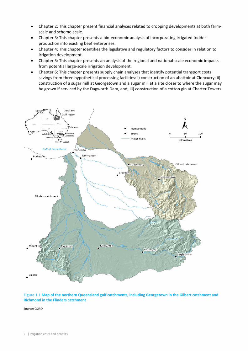
The more northern Gilbert catchment expands over nearly 47,000 km2 around the Gilbert-Einasleigh river system (Figure 1.1). Depending on the intensity of the wet season, the Gilbert-Einasleigh River has the sixth-highest discharge of any river in Australia, and its runoff totals about 2.2% of the total runoff from the whole country. Both the Gilbert and the Einasleigh Rivers rise in ancient uplands to the west of the Atherton Tableland in northern Queensland and discharge in the Gulf of Carpentaria.
The more southern Flinders catchment (Figure 1.1) covers an area of approximately 100,000 km². It is bordered in the north by the Flinders River which, at around 1,000 km, is the longest river in Queensland and the sixth longest river in Australia. The river rises in the Burra Range, part of the Great Dividing Range, 110 km northeast of Hughenden and flows in a westerly direction past Hughenden, Richmond and Julia Creek then northwest to the Gulf of Carpentaria 25 km west of Karumba, Queensland. The south of the catchment is bordered by the Selwyn Range.
The Gilbert and Flinders catchments have a semi-arid tropical climate, with high incidence of monsoon variability and occasional severe cyclones. As a result, seasonality of rainfall is the most defining characteristic of the climate of both catchments, with 93% and 88% of rainfall occurring during the wet season (November to April inclusive) in the Gilbert and Flinders catchments, respectively. Spatially, mean annual rainfall varies from about 1050 mm on the coast in the north of the Gilbert catchment to about 650 mm in the south-east of the catchment, and from about 800 mm on the coast in the north of the Flinders catchment to about 350 mm in the south of the catchment (Petheram and Yang, 2013). The climate of the Gilbert and Flinders catchments is described in more detail in a companion technical report in Petheram et al. (2013).
1.3 Structure of this report
This report is structured as follows: • Chapter 1: This chapter provides a brief overview of the report. Detailed background material
about the biophysical and human features of the catchments is not provided here. Rather, readers are advised to consult the Assessment’s catchment reports and the other technical reports of interest for detailed contextual information.
2 | Irrigation costs and benefits
• Chapter 2: This chapter present financial analyses related to cropping developments at both farm-scale and scheme-scale.
• Chapter 3: This chapter presents a bio-economic analysis of incorporating irrigated fodder production into existing beef enterprises.
• Chapter 4: This chapter identifies the legislative and regulatory factors to consider in relation to irrigation development.
• Chapter 5: This chapter presents an analysis of the regional and national-scale economic impacts from potential large-scale irrigation development.
• Chapter 6: This chapter presents supply chain analyses that identify potential transport costs savings from three hypothetical processing facilities: i) construction of an abattoir at Cloncurry; ii) construction of a sugar mill at Georgetown and a sugar mill at a site closer to where the sugar may be grown if serviced by the Dagworth Dam, and; iii) construction of a cotton gin at Charter Towers.
Figure 1.1 Map of the northern Queensland gulf catchments, including Georgetown in the Gilbert catchment and Richmond in the Flinders catchment
Source: CSIRO
Farm-scale and scheme-scale financial evaluation for irrigated cropping developments | 3
2 Farm-scale and scheme-scale financial evaluation for irrigated cropping developments
2.1 Introduction
This chapter introduces the analysis frameworks adopted in the Agricultural Resource Assessments for the Flinders and Gilbert catchments for the financial evaluation of irrigation developments at both the farm-scale and scheme-scale. These frameworks are then applied to generic development examples to illustrate the drivers of financial performance. Specific development options are reported as case studies in the Assessment’s catchment reports (Petheram et al., 2013 a,b) using the frameworks presented here.
The analysis of introducing irrigated fodder into an existing beef enterprise is reported in Chapter 3.
2.2 Discounted cash flow analysis framework
At both farm- and scheme-scale, financial evaluations (also known as investment evaluations) are conducted to ask whether an irrigation project offers an acceptable return from a funds-owner perspective. This framework does not extend to a full economic evaluation which involves considering costs and benefits that are ‘unpriced’ and not the subject of normal market transactions.
2.2.1 NET PRESENT VALUE
As new capital projects requiring equipment and infrastructure investment, irrigation projects are analysed over their lifetime costs and benefits. Costs and benefits occurring at different time periods are set on a comparable basis – i.e. they are expressed in real terms. In other words, they are expressed in constant dollars and increases in prices due to the general rate of inflation are not included in the values placed on future benefits and costs. When a cost stream has been subtracted from the benefit stream to give a net benefit stream, a discount rate is applied to yield a net present value (NPV) for the project. The net present value is used to facilitate comparisons between options. The option with the largest NPV will be preferred.
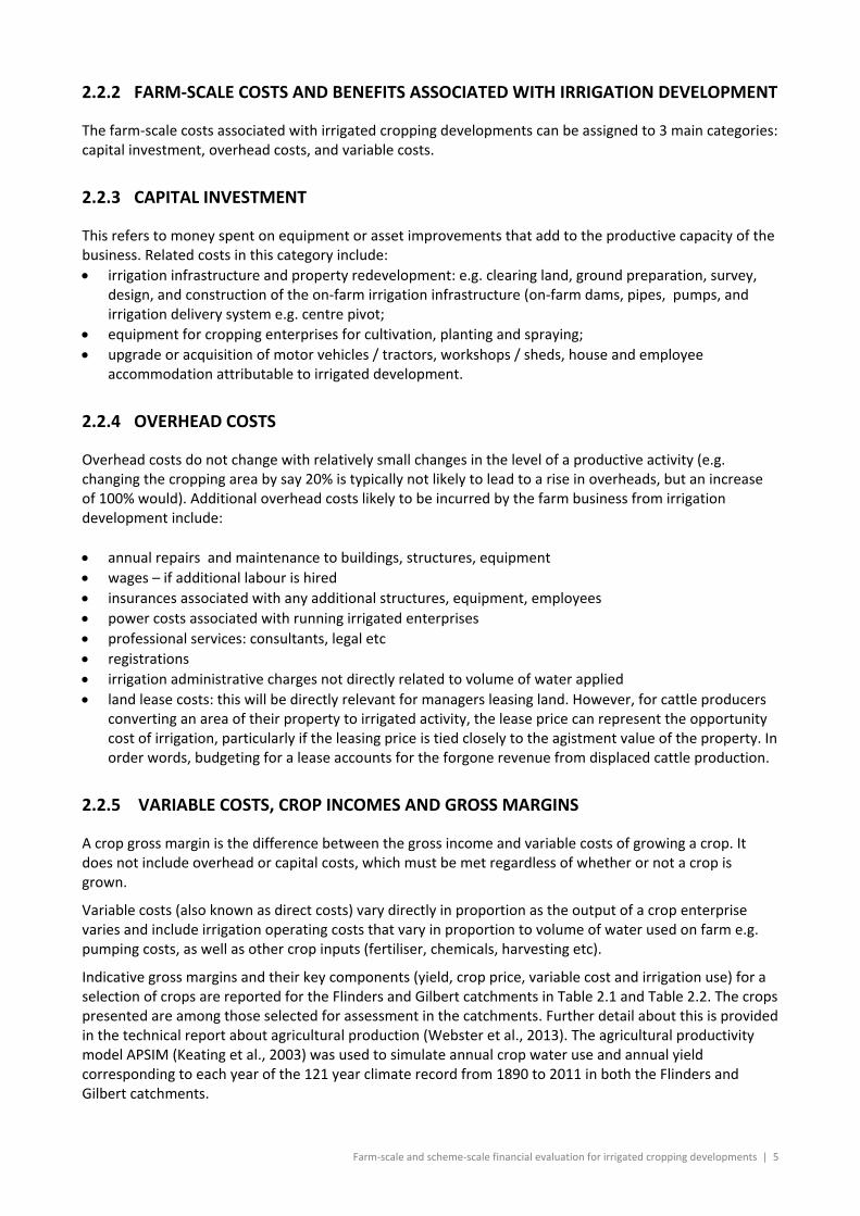
Net present value is expressed as follows:
Where:
Bn = project benefits in year n expressed in constant dollars
Cn = project costs in year n expressed in constant dollars
r= real, pre-tax discount rate
N= number of years that costs and benefits are produced.
Under this decision rule, a project is potentially viable if the NPV is greater than zero.
4 | Irrigation costs and benefits
Internal rate of return
The internal rate of return (IRR) is presented as supplementary information to the NPV. The IRR is the discount rate which causes the NPV to become zero. The project’s IRR needs to be above the discount rate for the project to be considered viable.
Project period
For the farm-scale investment analysis, the project is assessed over 15 years. Where a project option includes an on-farm water storage (e.g. ring tank), this results in the project life being shorter than asset life of 40 years for an on-farm storage. However, it reflects the working asset life of other on-farm assets, such as irrigation and cultivation equipment.
For the scheme-scale analysis, a project period of 30 years was selected. This project life has been adopted to reflect the life of principal asset, which is in this case the scheme infrastructure (storage, weirs, channels). The 30 year project life is also less than the actual working life of these assets, but once a project life has exceeded 30 years the analysis will be relatively insensitive to the choice of a longer project period due to the discounting of future costs and benefits.
The NSW Government Guidelines for Economic Appraisal and Guidelines for Financial and Economic Evaluation of New Water Infrastructure in Queensland advise that there is little justification for extending the project period beyond 30 years.
Discount rate
A real, pre-tax discount rate of 7% was selected for this analysis. It was assumed that this rate reflects what a private sector business would seek from an investment with risk. Additional analyses at the farm-scale were also conducted at 5% for sensitivity testing purposes. This discount rate of 5% is closer to rates of return experienced in agriculture in recent years.
Replacement of assets
In the scheme-scale analysis, as some assets in the evaluation period have lives shorter than the project period (e.g. pump equipment with an asset life of 15 years), the replacement of these has been incorporated into the analysis. The assumption made is that such assets will be replaced at their end of their life with an exact replacement until the end of the assessed project period of 30 years. These costs have been accounted for in full in the actual year of their replacement. To continue the pumping equipment example, this means that pumps were replaced in year 16 with the expectation that their working life would end at year 30. This approach assumes that the technology and cost does not change over time, when in reality this may not be the case.
Residual value
A residual value has been calculated for project assets where the life of the project exceeds the planning period. There are multiple accepted ways to calculate residual value. The approach adopted in this analysis has been to calculate a residual value based on the straight-line depreciation method. To calculate this, the value of the constructed assets (scheme storage and irrigated area works) is equated to the purchase and development price, divided by the asset life in years, and then multiplied by the remaining years of asset life. Using this approach means that if an asset has a 40 year life then its value at the end of year 15, for example, is the asset value/40 x 25, with 25 representing the remaining years of life. This approach assumes that the services derived from the asset do not degrade over time, and a maintenance budget is allowed for in the analysis, consistent with the assumption. In reality, farm dams can experience degradation in the asset value from issues such as silting, leaks and weed incursion.
Farm-scale and scheme-scale financial evaluation for irrigated cropping developments | 5
2.2.2 FARM-SCALE COSTS AND BENEFITS ASSOCIATED WITH IRRIGATION DEVELOPMENT
The farm-scale costs associated with irrigated cropping developments can be assigned to 3 main categories: capital investment, overhead costs, and variable costs.
2.2.3 CAPITAL INVESTMENT
This refers to money spent on equipment or asset improvements that add to the productive capacity of the business. Related costs in this category include: • irrigation infrastructure and property redevelopment: e.g. clearing land, ground preparation, survey,
design, and construction of the on-farm irrigation infrastructure (on-farm dams, pipes, pumps, and irrigation delivery system e.g. centre pivot;
• equipment for cropping enterprises for cultivation, planting and spraying; • upgrade or acquisition of motor vehicles / tractors, workshops / sheds, house and employee
accommodation attributable to irrigated development.
2.2.4 OVERHEAD COSTS
Overhead costs do not change with relatively small changes in the level of a productive activity (e.g. changing the cropping area by say 20% is typically not likely to lead to a rise in overheads, but an increase of 100% would). Additional overhead costs likely to be incurred by the farm business from irrigation development include: • annual repairs and maintenance to buildings, structures, equipment • wages – if additional labour is hired • insurances associated with any additional structures, equipment, employees • power costs associated with running irrigated enterprises • professional services: consultants, legal etc • registrations • irrigation administrative charges not directly related to volume of water applied • land lease costs: this will be directly relevant for managers leasing land. However, for cattle producers
converting an area of their property to irrigated activity, the lease price can represent the opportunity cost of irrigation, particularly if the leasing price is tied closely to the agistment value of the property. In order words, budgeting for a lease accounts for the forgone revenue from displaced cattle production.
2.2.5 VARIABLE COSTS, CROP INCOMES AND GROSS MARGINS
A crop gross margin is the difference between the gross income and variable costs of growing a crop. It does not include overhead or capital costs, which must be met regardless of whether or not a crop is grown.
Variable costs (also known as direct costs) vary directly in proportion as the output of a crop enterprise varies and include irrigation operating costs that vary in proportion to volume of water used on farm e.g. pumping costs, as well as other crop inputs (fertiliser, chemicals, harvesting etc).
Indicative gross margins and their key components (yield, crop price, variable cost and irrigation use) for a selection of crops are reported for the Flinders and Gilbert catchments in Table 2.1 and Table 2.2. The crops presented are among those selected for assessment in the catchments. Further detail about this is provided in the technical report about agricultural production (Webster et al., 2013). The agricultural productivity model APSIM (Keating et al., 2003) was used to simulate annual crop water use and annual yield corresponding to each year of the 121 year climate record from 1890 to 2011 in both the Flinders and Gilbert catchments.
6 | Irrigation costs and benefits
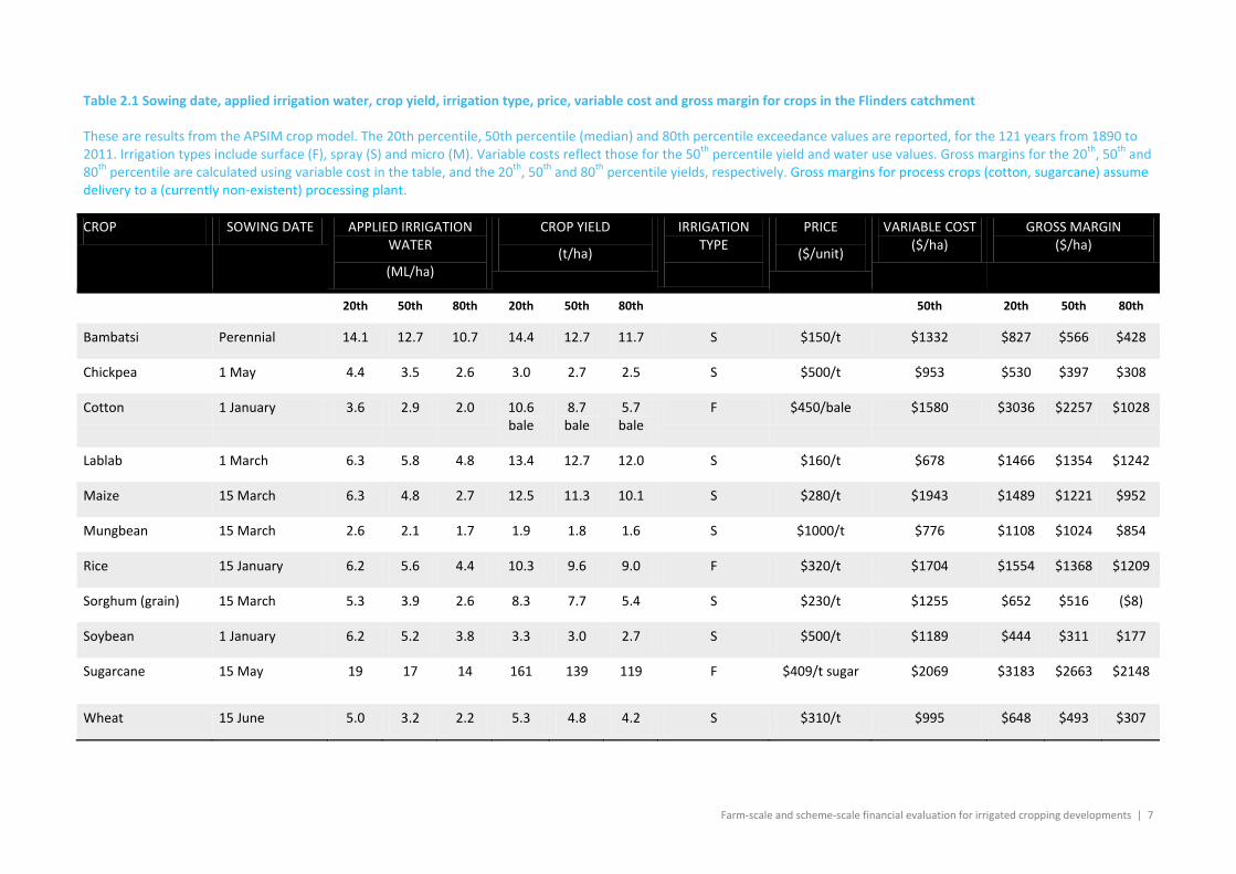
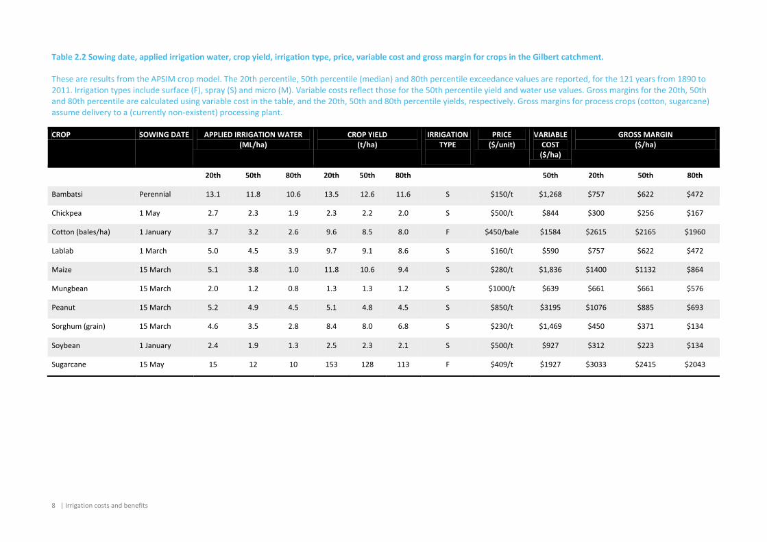
The tables show estimates of potential crop yields at the 20th, 50th and 80th percentile exceedance averaged over all modelled years (1890-2011) for the Flinders and Gilbert catchments. The use of 121 seasons of data provides for robust assessments of both median yield and the variability that can be expected about the average. The 20th percentile exceedance values represent the yield that is exceeded in 20% of all years (i.e. in 20% of years the yield will be higher than this value). Similarly, the 80th percentile exceedance values represent the yield that is exceeded in 80% of years (i.e. in 80% of years the yield will be higher than this value).
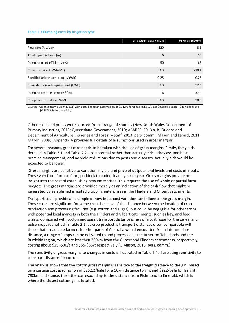
Gross margins are similarly presented. Gross incomes were calculated using the modelled 20th, 50th and 80th percentile exceedance crop yield values. These modelled crop yield values were used to calculate tonnage-related variable costs (e.g. cartage, levies, harvesting) which were converted to a $ per hectare cost and added to other variable costs of production. Pumping costs were calculated using the modelled median applied irrigation water (ML/ha), the irrigation system assigned to the crop (surface irrigation – furrow or spray – centre pivot), and the diesel cost assumptions in Table 2.3. It is important to note that the gross margins exclude the costs of a water charge for the purposes of this analysis. It is, however, typically a variable cost and an irrigator should add this to the variable costs in the gross margin calculation if water is being purchased from a water supplier.
Farm-scale and scheme-scale financial evaluation for irrigated cropping developments | 7
Table 2.1 Sowing date, applied irrigation water, crop yield, irrigation type, price, variable cost and gross margin for crops in the Flinders catchment
These are results from the APSIM crop model. The 20th percentile, 50th percentile (median) and 80th percentile exceedance values are reported, for the 121 years from 1890 to 2011. Irrigation types include surface (F), spray (S) and micro (M). Variable costs reflect those for the 50th percentile yield and water use values. Gross margins for the 20th, 50th and 80th percentile are calculated using variable cost in the table, and the 20th, 50th and 80th percentile yields, respectively. Gross margins for process crops (cotton, sugarcane) assume delivery to a (currently non-existent) processing plant.
CROP SOWING DATE APPLIED IRRIGATION WATER
(ML/ha)
CROP YIELD
(t/ha)
IRRIGATION TYPE
PRICE
($/unit)
VARIABLE COST ($/ha)
GROSS MARGIN ($/ha)
20th 50th 80th 20th 50th 80th 50th 20th 50th 80th
Bambatsi Perennial 14.1 12.7 10.7 14.4 12.7 11.7 S $150/t $1332 $827 $566 $428
Chickpea 1 May 4.4 3.5 2.6 3.0 2.7 2.5 S $500/t $953 $530 $397 $308
Cotton 1 January 3.6 2.9 2.0 10.6 bale
8.7 bale
5.7 bale
F $450/bale $1580 $3036 $2257 $1028
Lablab 1 March 6.3 5.8 4.8 13.4 12.7 12.0 S $160/t $678 $1466 $1354 $1242
Maize 15 March 6.3 4.8 2.7 12.5 11.3 10.1 S $280/t $1943 $1489 $1221 $952
Mungbean 15 March 2.6 2.1 1.7 1.9 1.8 1.6 S $1000/t $776 $1108 $1024 $854
Rice 15 January 6.2 5.6 4.4 10.3 9.6 9.0 F $320/t $1704 $1554 $1368 $1209
Sorghum (grain) 15 March 5.3 3.9 2.6 8.3 7.7 5.4 S $230/t $1255 $652 $516 ($8)
Soybean 1 January 6.2 5.2 3.8 3.3 3.0 2.7 S $500/t $1189 $444 $311 $177
Sugarcane 15 May 19 17 14 161 139 119 F $409/t sugar $2069 $3183 $2663 $2148
Wheat 15 June 5.0 3.2 2.2 5.3 4.8 4.2 S $310/t $995 $648 $493 $307
8 | Irrigation costs and benefits
Table 2.2 Sowing date, applied irrigation water, crop yield, irrigation type, price, variable cost and gross margin for crops in the Gilbert catchment.
These are results from the APSIM crop model. The 20th percentile, 50th percentile (median) and 80th percentile exceedance values are reported, for the 121 years from 1890 to 2011. Irrigation types include surface (F), spray (S) and micro (M). Variable costs reflect those for the 50th percentile yield and water use values. Gross margins for the 20th, 50th and 80th percentile are calculated using variable cost in the table, and the 20th, 50th and 80th percentile yields, respectively. Gross margins for process crops (cotton, sugarcane) assume delivery to a (currently non-existent) processing plant.
CROP SOWING DATE APPLIED IRRIGATION WATER (ML/ha)
CROP YIELD (t/ha)
IRRIGATION TYPE
PRICE ($/unit)
VARIABLE COST ($/ha)
GROSS MARGIN ($/ha)
20th 50th 80th 20th 50th 80th 50th 20th 50th 80th
Bambatsi Perennial 13.1 11.8 10.6 13.5 12.6 11.6 S $150/t $1,268 $757 $622 $472
Chickpea 1 May 2.7 2.3 1.9 2.3 2.2 2.0 S $500/t $844 $300 $256 $167
Cotton (bales/ha) 1 January 3.7 3.2 2.6 9.6 8.5 8.0 F $450/bale $1584 $2615 $2165 $1960
Lablab 1 March 5.0 4.5 3.9 9.7 9.1 8.6 S $160/t $590 $757 $622 $472
Maize 15 March 5.1 3.8 1.0 11.8 10.6 9.4 S $280/t $1,836 $1400 $1132 $864
Mungbean 15 March 2.0 1.2 0.8 1.3 1.3 1.2 S $1000/t $639 $661 $661 $576
Peanut 15 March 5.2 4.9 4.5 5.1 4.8 4.5 S $850/t $3195 $1076 $885 $693
Sorghum (grain) 15 March 4.6 3.5 2.8 8.4 8.0 6.8 S $230/t $1,469 $450 $371 $134
Soybean 1 January 2.4 1.9 1.3 2.5 2.3 2.1 S $500/t $927 $312 $223 $134
Sugarcane 15 May 15 12 10 153 128 113 F $409/t $1927 $3033 $2415 $2043
Chapter 2 Farm-scale and scheme-scale financial evaluation for irrigated cropping developments | 9
Table 2.3 Pumping costs by irrigation type
SURFACE IRRIGATING CENTRE PIVOTS
Flow rate (ML/day) 120 8.6
Total dynamic head (m) 6 50
Pumping plant efficiency (%) 50 66
Power required (kWh/ML) 33.3 210.4
Specific fuel consumption (L/kWh) 0.25 0.25
Equivalent diesel requirement (L/ML) 8.3 52.6
Pumping cost – electricity $/ML 6 37.9
Pumping cost – diesel $/ML 9.3 58.9
Source: Adapted from Culpitt (2011) with costs based on assumption of $1.12/L for diesel ($1.50/L less $0.38c/L rebate) $ for diesel and $0.18/kWh for electricity.
Other costs and prices were sourced from a range of sources (New South Wales Department of Primary Industries, 2013; Queensland Government, 2010; ABARES, 2013 a, b; Queensland Department of Agriculture, Fisheries and Forestry staff, 2013, pers. comm.; Mason and Larard, 2011; Mason, 2009). Appendix A provides full details of assumptions used in gross margins.
For several reasons, great care needs to be taken with the use of gross margins. Firstly, the yields detailed in Table 2.1 and Table 2.2 are potential rather than actual yields – they assume best practice management, and no yield reductions due to pests and diseases. Actual yields would be expected to be lower.
Gross margins are sensitive to variation in yield and price of outputs, and levels and costs of inputs. These vary from farm to farm, paddock to paddock and year to year. Gross margins provide no insight into the cost of establishing new enterprises. This requires the use of whole or partial farm budgets. The gross margins are provided merely as an indication of the cash flow that might be generated by established irrigated cropping enterprises in the Flinders and Gilbert catchments.
Transport costs provide an example of how input cost variation can influence the gross margin. These costs are significant for some crops because of the distance between the location of crop production and processing facilities (e.g. cotton and sugar), but could be negligible for other crops with potential local markets in both the Flinders and Gilbert catchments, such as hay, and feed grains. Compared with cotton and sugar, transport distance is less of a cost issue for the cereal and pulse crops identified in Table 2.1. as crop product is transport distances often comparable with those that broad acre farmers in other parts of Australia would encounter. At an intermediate distance, a range of crops can be delivered to and processed at the Atherton Tablelands and the Burdekin region, which are less then 300km from the Gilbert and Flinders catchments, respectively, costing about $25 -$30/t and $55-$65/t respectively (G Mason, 2013, pers. comm.).
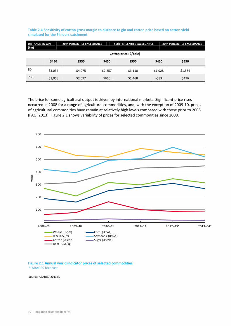
The sensitivity of gross margins to changes in costs is illustrated in Table 2.4, illustrating sensitivity to transport distance for cotton.
The analysis shows that the cotton gross margin is sensitive to the freight distance to the gin (based on a cartage cost assumption of $25.12/bale for a 50km distance to gin, and $222/bale for freight 780km in distance, the latter corresponding to the distance from Richmond to Emerald, which is where the closest cotton gin is located.
10 | Irrigation costs and benefits
Table 2.4 Sensitivity of cotton gross margin to distance to gin and cotton price based on cotton yield simulated for the Flinders catchment.
DISTANCE TO GIN (km)
20th PERCENTILE EXCEEDANCE 50th PERCENTILE EXCEEDANCE 80th PERCENTILE EXCEEDANCE
Cotton price ($/bale)
$450 $550 $450 $550 $450 $550
50 $3,036 $4,075 $2,257 $3,110 $1,028 $1,586
780 $1,058 $2,097 $615 $1,468 -$83 $476
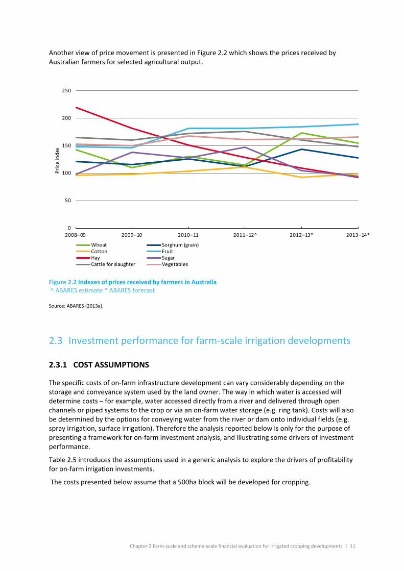
The price for some agricultural output is driven by international markets. Significant price rises occurred in 2008 for a range of agricultural commodities, and, with the exception of 2009-10, prices of agricultural commodities have remain at relatively high levels compared with those prior to 2008 (FAO, 2013). Figure 2.1 shows variability of prices for selected commodities since 2008.
Figure 2.1 Annual world indicator prices of selected commodities * ABARES forecast
Source: ABARES (2013a).
100
200
300
400
500
600
700
2008–09 2009–10 2010–11 2011–12 2012–13* 2013–14*
Valu
e
Wheat (US$/t) Corn (US$/t)Rice (US$/t) Soybeans (US$/t)Cotton (USc/lb) Sugar (USc/lb)Beef (USc/kg)
Chapter 2 Farm-scale and scheme-scale financial evaluation for irrigated cropping developments | 11
Another view of price movement is presented in Figure 2.2 which shows the prices received by Australian farmers for selected agricultural output.
Figure 2.2 Indexes of prices received by farmers in Australia ^ ABARES estimate * ABARES forecast
Source: ABARES (2013a).
2.3 Investment performance for farm-scale irrigation developments
2.3.1 COST ASSUMPTIONS
The specific costs of on-farm infrastructure development can vary considerably depending on the storage and conveyance system used by the land owner. The way in which water is accessed will determine costs – for example, water accessed directly from a river and delivered through open channels or piped systems to the crop or via an on-farm water storage (e.g. ring tank). Costs will also be determined by the options for conveying water from the river or dam onto individual fields (e.g. spray irrigation, surface irrigation). Therefore the analysis reported below is only for the purpose of presenting a framework for on-farm investment analysis, and illustrating some drivers of investment performance.
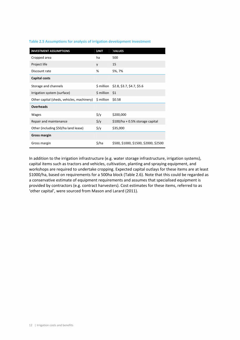
Table 2.5 introduces the assumptions used in a generic analysis to explore the drivers of profitability for on-farm irrigation investments.
The costs presented below assume that a 500ha block will be developed for cropping.
0
50
100
150
200
250
2008–09 2009–10 2010–11 2011–12^ 2012–13* 2013–14*
Pric
e in
dex
Wheat Sorghum (grain)Cotton FruitHay SugarCattle for slaughter Vegetables
12 | Irrigation costs and benefits
Table 2.5 Assumptions for analysis of irrigation development investment
INVESTMENT ASSUMPTIONS UNIT VALUES
Cropped area ha 500
Project life y 15
Discount rate % 5%, 7%
Capital costs
Storage and channels $ million $2.8, $3.7, $4.7, $5.6
Irrigation system (surface) $ million $1
Other capital (sheds, vehicles, machinery) $ million $0.58
Overheads
Wages $/y $200,000
Repair and maintenance $/y $100/ha + 0.5% storage capital
Other (including $50/ha land lease) $/y $35,000
Gross margin
Gross margin $/ha $500, $1000, $1500, $2000, $2500
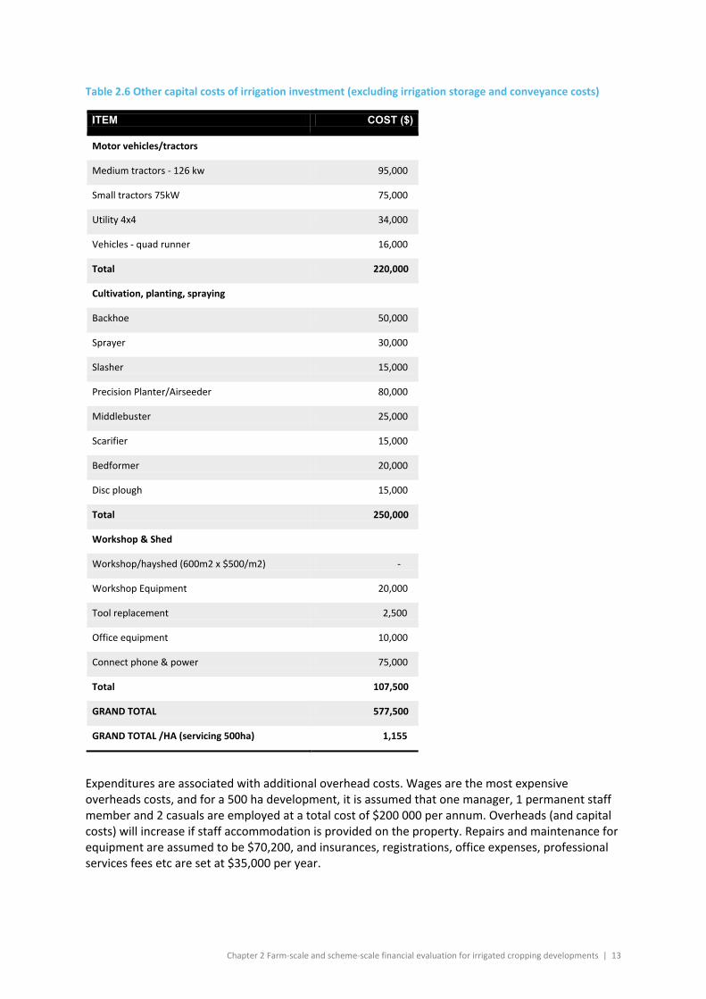
In addition to the irrigation infrastructure (e.g. water storage infrastructure, irrigation systems), capital items such as tractors and vehicles, cultivation, planting and spraying equipment, and workshops are required to undertake cropping. Expected capital outlays for these items are at least $1000/ha, based on requirements for a 500ha block (Table 2.6). Note that this could be regarded as a conservative estimate of equipment requirements and assumes that specialised equipment is provided by contractors (e.g. contract harvesters). Cost estimates for these items, referred to as ‘other capital’, were sourced from Mason and Larard (2011).
Chapter 2 Farm-scale and scheme-scale financial evaluation for irrigated cropping developments | 13
Table 2.6 Other capital costs of irrigation investment (excluding irrigation storage and conveyance costs)
ITEM COST ($)
Motor vehicles/tractors
Medium tractors - 126 kw 95,000
Small tractors 75kW 75,000
Utility 4x4 34,000
Vehicles - quad runner 16,000
Total 220,000
Cultivation, planting, spraying
Backhoe 50,000
Sprayer 30,000
Slasher 15,000
Precision Planter/Airseeder 80,000
Middlebuster 25,000
Scarifier 15,000
Bedformer 20,000
Disc plough 15,000
Total 250,000
Workshop & Shed
Workshop/hayshed (600m2 x $500/m2) -
Workshop Equipment 20,000
Tool replacement 2,500
Office equipment 10,000
Connect phone & power 75,000
Total 107,500
GRAND TOTAL 577,500
GRAND TOTAL /HA (servicing 500ha) 1,155
Expenditures are associated with additional overhead costs. Wages are the most expensive overheads costs, and for a 500 ha development, it is assumed that one manager, 1 permanent staff member and 2 casuals are employed at a total cost of $200 000 per annum. Overheads (and capital costs) will increase if staff accommodation is provided on the property. Repairs and maintenance for equipment are assumed to be $70,200, and insurances, registrations, office expenses, professional services fees etc are set at $35,000 per year.
14 | Irrigation costs and benefits
2.3.2 FINANCIAL ANALYSIS
For the analysis reported here the project is an investment in a ring tank (on-farm dam) constructed to access water harvesting opportunities. Capacities ranging from 952 to 3,810ML and surface irrigation ($2000/ha) were included in the analysis. The four storage sizes (Table 2.5) correspond to effective volumes ranging from an allocation of 500ML (1ML/ha) to 2000ML (4ML/ha) after evaporation and seepage losses from the storage (30%) and irrigation losses of 25% are accounted for. Losses can be either higher or lower depending on the rate of seepage from the storage, the duration of water storage, and the irrigation system used. For example, to provide an effective volume of 2000 ML, reducing the irrigation water loss from 25 to 15% can reduce the capacity requirement of the storage from 3,810 to 3,360ML – a cost reduction of about $450 000, although the additional capital costs of a more efficient irrigation system to achieve this - such as a centre pivot irrigator ($4,500/ha) - would exceed the saving enabled by the smaller dam. The storage construction cost was based on earthworks construction costs of $ 4/m3 and a 4:1 storage to excavation ratio.
The storage was assigned an economic life of 40 years. The straight-line depreciation method was used to calculate the residual value at the end of 15 years. Costs and revenue streams were accounted for over a 15 year investment period and discounted at a real discount rate of 5% and 7% in order to calculate a NPV.
The impact of capital cost on NPV was explored under an annual crop gross margin of $1500 (Table 2.7), which is achievable from a range of crops in Table 2.1 It is assumed that this gross margin is generated in every year of the investment period. It is not suggested that this reliability of income is achievable in practice, however, this analysis is intended to be illustrative only of the magnitude of investment net returns under different capital costs.
The capital costs of water storage infrastructure significantly impacts on the viability of the irrigation investment. For the 3,810 ML (largest) storage, and a 5% discount rate, a gross margin of $1509 is required to break even (i.e. return an NPV of zero). Table 2.1 and Table 2.2. shows that gross margins around this value, that can be achieved with the storage’s corresponding allocation of 4ML/ha, are possible for a very limited range of crops (e.g. cotton, maize, lab lab hay), and with varying degrees of reliability every year under the set of price, input cost and yield combinations presented.
Investment returns are higher with smaller, less expensive farm-dams, however over the cropping area assumed (500ha), this further restricts the set of crops that could be grown to those with lower ML/ha water use, but still able to generate the gross margin assumed in the analysis. (e.g. cotton, with a median water use of 2.9ML/ha and median gross margin of $2413/ha). This analysis shows that that larger storage capacity can increase cropping flexibility by allowing a greater range of crops to be grown, but that the payoffs are not generated under the gross margin assumption of $1500/ha.
Table 2.7 and Figure 2.3 illustrate the impact of changing investment assumptions:
• A higher discount rate reduces the investment NPV. • The NPV is further reduced by not assigning a residual value to the asset at the end of the
investment period. • Constructing the infrastructure over three years, with partial production occurring during
this time, and full crop production occurring in year 3 slightly decreases the NPV.
Crop gross margins are sensitive to commodity price movements and yield variation, which in turn reflects a range of production risks, including water reliability. Likewise, the performance of the overall investment is sensitive to gross margin (Table 2.8). With reduced gross margins of $1000/ha
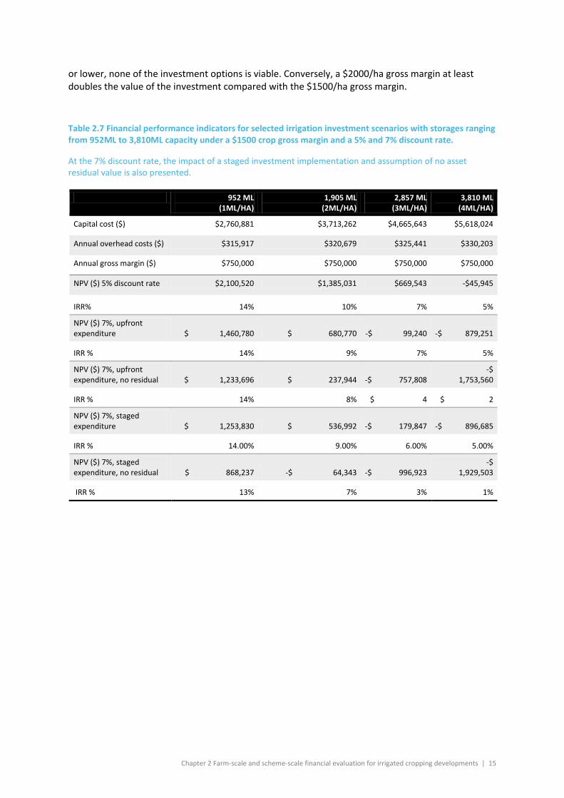
Chapter 2 Farm-scale and scheme-scale financial evaluation for irrigated cropping developments | 15
or lower, none of the investment options is viable. Conversely, a $2000/ha gross margin at least doubles the value of the investment compared with the $1500/ha gross margin.
Table 2.7 Financial performance indicators for selected irrigation investment scenarios with storages ranging from 952ML to 3,810ML capacity under a $1500 crop gross margin and a 5% and 7% discount rate.
At the 7% discount rate, the impact of a staged investment implementation and assumption of no asset residual value is also presented.
952 ML (1ML/HA)
1,905 ML (2ML/HA)
2,857 ML (3ML/HA)
3,810 ML (4ML/HA)
Capital cost ($) $2,760,881 $3,713,262 $4,665,643 $5,618,024
Annual overhead costs ($) $315,917 $320,679 $325,441 $330,203
Annual gross margin ($) $750,000 $750,000 $750,000 $750,000
NPV ($) 5% discount rate $2,100,520 $1,385,031 $669,543 -$45,945
IRR% 14% 10% 7% 5%
NPV ($) 7%, upfront expenditure $ 1,460,780 $ 680,770 -$ 99,240 -$ 879,251
IRR % 14% 9% 7% 5%
NPV ($) 7%, upfront expenditure, no residual $ 1,233,696 $ 237,944 -$ 757,808
-$ 1,753,560
IRR % 14% 8% $ 4 $ 2
NPV ($) 7%, staged expenditure $ 1,253,830 $ 536,992 -$ 179,847 -$ 896,685
IRR % 14.00% 9.00% 6.00% 5.00%
NPV ($) 7%, staged expenditure, no residual $ 868,237 -$ 64,343 -$ 996,923
-$ 1,929,503
IRR % 13% 7% 3% 1%
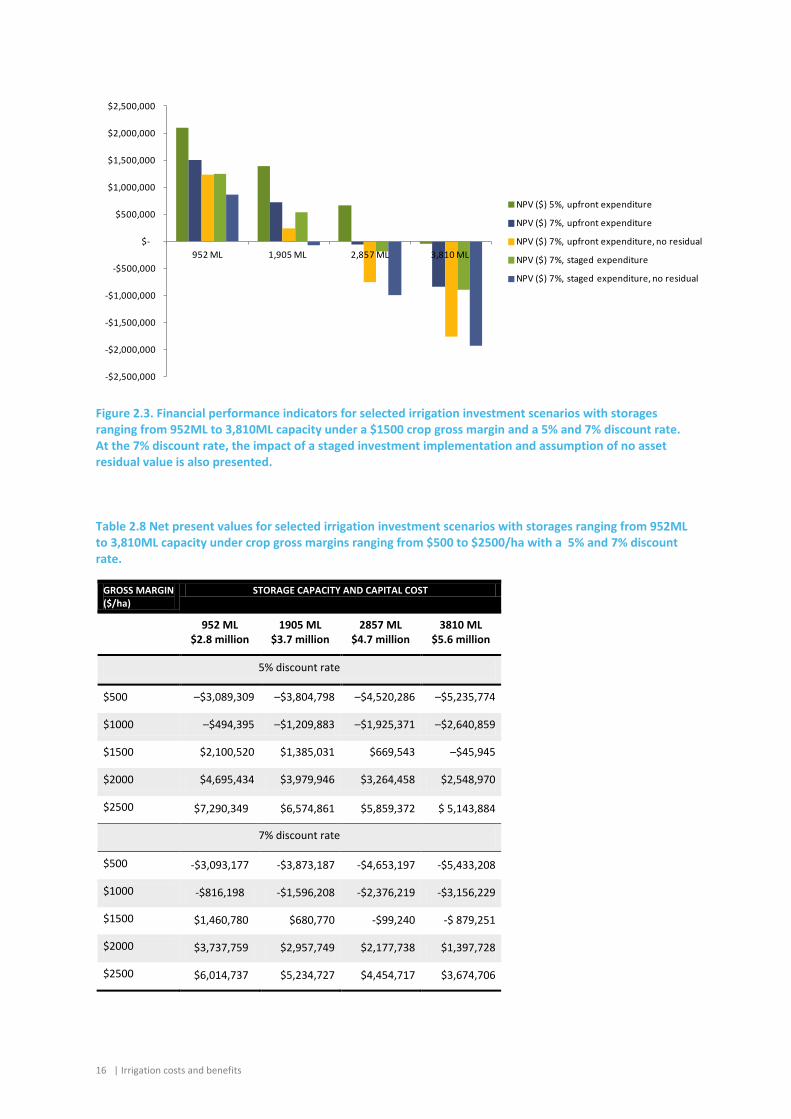
16 | Irrigation costs and benefits
Figure 2.3. Financial performance indicators for selected irrigation investment scenarios with storages ranging from 952ML to 3,810ML capacity under a $1500 crop gross margin and a 5% and 7% discount rate. At the 7% discount rate, the impact of a staged investment implementation and assumption of no asset residual value is also presented.
Table 2.8 Net present values for selected irrigation investment scenarios with storages ranging from 952ML to 3,810ML capacity under crop gross margins ranging from $500 to $2500/ha with a 5% and 7% discount rate.
GROSS MARGIN ($/ha)
STORAGE CAPACITY AND CAPITAL COST
952 ML $2.8 million
1905 ML $3.7 million
2857 ML $4.7 million
3810 ML $5.6 million
5% discount rate
$500 –$3,089,309 –$3,804,798 –$4,520,286 –$5,235,774
$1000 –$494,395 –$1,209,883 –$1,925,371 –$2,640,859
$1500 $2,100,520 $1,385,031 $669,543 –$45,945
$2000 $4,695,434 $3,979,946 $3,264,458 $2,548,970
$2500 $7,290,349 $6,574,861 $5,859,372 $ 5,143,884
7% discount rate
$500 -$3,093,177 -$3,873,187 -$4,653,197 -$5,433,208
$1000 -$816,198 -$1,596,208 -$2,376,219 -$3,156,229
$1500 $1,460,780 $680,770 -$99,240 -$ 879,251
$2000 $3,737,759 $2,957,749 $2,177,738 $1,397,728
$2500 $6,014,737 $5,234,727 $4,454,717 $3,674,706
-$2,500,000
-$2,000,000
-$1,500,000
-$1,000,000
-$500,000
$-
$500,000
$1,000,000
$1,500,000
$2,000,000
$2,500,000
952 ML 1,905 ML 2,857 ML 3,810 ML
NPV ($) 5%, upfront expenditure
NPV ($) 7%, upfront expenditure
NPV ($) 7%, upfront expenditure, no residual
NPV ($) 7%, staged expenditure
NPV ($) 7%, staged expenditure, no residual
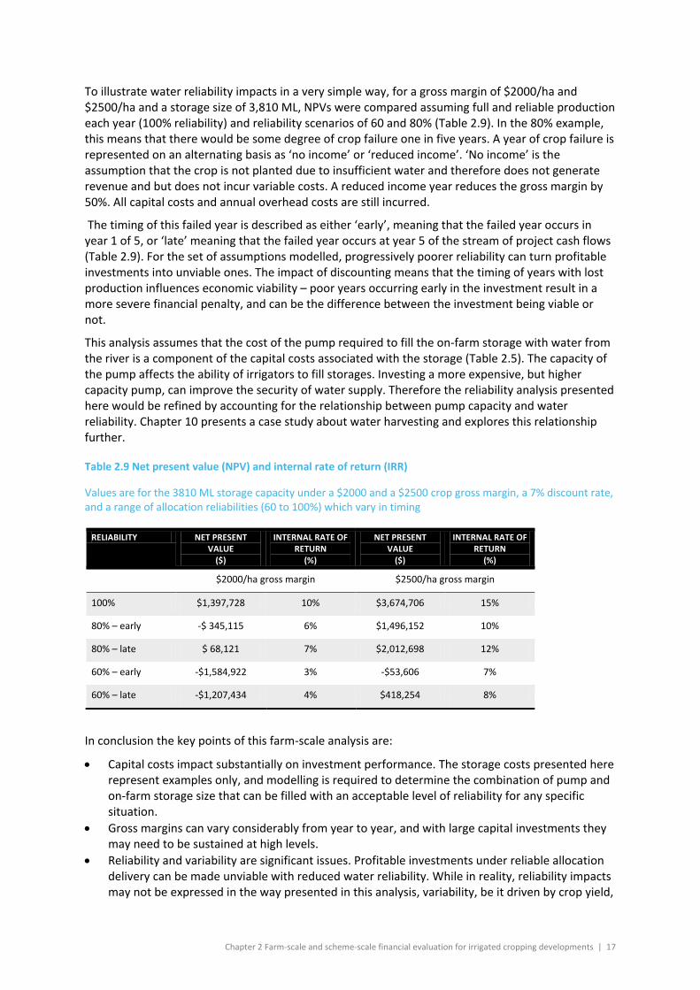
Chapter 2 Farm-scale and scheme-scale financial evaluation for irrigated cropping developments | 17
To illustrate water reliability impacts in a very simple way, for a gross margin of $2000/ha and $2500/ha and a storage size of 3,810 ML, NPVs were compared assuming full and reliable production each year (100% reliability) and reliability scenarios of 60 and 80% (Table 2.9). In the 80% example, this means that there would be some degree of crop failure one in five years. A year of crop failure is represented on an alternating basis as ‘no income’ or ‘reduced income’. ‘No income’ is the assumption that the crop is not planted due to insufficient water and therefore does not generate revenue and but does not incur variable costs. A reduced income year reduces the gross margin by 50%. All capital costs and annual overhead costs are still incurred.
The timing of this failed year is described as either ‘early’, meaning that the failed year occurs in year 1 of 5, or ‘late’ meaning that the failed year occurs at year 5 of the stream of project cash flows (Table 2.9). For the set of assumptions modelled, progressively poorer reliability can turn profitable investments into unviable ones. The impact of discounting means that the timing of years with lost production influences economic viability – poor years occurring early in the investment result in a more severe financial penalty, and can be the difference between the investment being viable or not.
This analysis assumes that the cost of the pump required to fill the on-farm storage with water from the river is a component of the capital costs associated with the storage (Table 2.5). The capacity of the pump affects the ability of irrigators to fill storages. Investing a more expensive, but higher capacity pump, can improve the security of water supply. Therefore the reliability analysis presented here would be refined by accounting for the relationship between pump capacity and water reliability. Chapter 10 presents a case study about water harvesting and explores this relationship further.
Table 2.9 Net present value (NPV) and internal rate of return (IRR)
Values are for the 3810 ML storage capacity under a $2000 and a $2500 crop gross margin, a 7% discount rate, and a range of allocation reliabilities (60 to 100%) which vary in timing
RELIABILITY NET PRESENT VALUE
($)
INTERNAL RATE OF RETURN
(%)
NET PRESENT VALUE
($)
INTERNAL RATE OF RETURN
(%)
$2000/ha gross margin $2500/ha gross margin
100% $1,397,728 10% $3,674,706 15%
80% – early -$ 345,115 6% $1,496,152 10%
80% – late $ 68,121 7% $2,012,698 12%
60% – early -$1,584,922 3% -$53,606 7%
60% – late -$1,207,434 4% $418,254 8%
In conclusion the key points of this farm-scale analysis are:
• Capital costs impact substantially on investment performance. The storage costs presented here represent examples only, and modelling is required to determine the combination of pump and on-farm storage size that can be filled with an acceptable level of reliability for any specific situation.
• Gross margins can vary considerably from year to year, and with large capital investments they may need to be sustained at high levels.
• Reliability and variability are significant issues. Profitable investments under reliable allocation delivery can be made unviable with reduced water reliability. While in reality, reliability impacts may not be expressed in the way presented in this analysis, variability, be it driven by crop yield,
18 | Irrigation costs and benefits
commodity price or water availability, can result in years of low or negative annual net margins, even if the investment is profitable over a longer-term period. The timing of variability matters – poor yield outcomes early in the life of the investment will further disadvantage the investment performance.
• This analysis is an introduction to the costs incurred at the farm-scale for irrigated cropping. It also introduces the impacts on net revenues of factors such as changing the discount rate, gross margin, and reliability of water supplies. The analysis is generic only, and is limited to the exploration of net returns arising from a ring tank investment. In the next section, farm-scale investment performance is further explored under a different situation, where irrigation water is supplied through an irrigation development project not requiring investment in individual farm dams.
2.4 Investment performance for scheme-scale irrigation developments
2.4.1 EVALUATION OF WATER INFRASTRUCTURE INVESTMENTS AND WATER PRICING PRINCIPLES
The Guidelines for Financial and Economic Evaluation of New Water Infrastructure in Queensland (the Guidelines; Queensland Government, 2000) provide a framework for the financial and economic assessment component of new water infrastructure investments in Queensland (including extensions to existing water infrastructure). Importantly, they require a financial and economic assessment be completed for water investment projects so that not only is the economic viability of the project established, but an estimate of the expected cost recovery of the project is also ascertained. This is important in relation to water pricing.
The Guidelines (Queensland Government, 2000) apply to Queensland Government Departments, statutory authorities and commercialised business units that are contemplating investments in water infrastructure. They are also applicable to a Government Owned Corporation or a private sector entity where a request is made to the Queensland Government for funding or where the Queensland Government is requested to assume some level of project risk.
Financial assessment is used to determine the commercial viability (profitability) of a project from a developer’s, or fund owner’s, perspective, whereas economic assessment determines the net benefits of a project to the economy and society as a whole. Given the purpose and objectives of financial and economic assessment are different, it will not always be the case that a project which proves to be financially viable will be economically viable and vice versa.
Where a project is not financially viable (in other words, the NPV of the project is less than zero), there may be a justification for the government to contribute funds towards new infrastructure in the form of Community Service Obligations (Community Service Obligations: A Policy Framework) (CSO; Queensland Government, 1999). The CSO specifies that the financial support for new infrastructure will be considered only in exceptional circumstances, for example where water prices are unable to at least cover the costs of assuring the ongoing financial viability of the development (DNRME 2004). To be considered as being eligible for Government CSOs, a project (that is, an irrigation development) should at least be able to cover the direct costs of providing the service (i.e. operational, maintenance and administrative costs, asset consumption (i.e. future asset refurbishment and replacement), externalities, taxes, interest costs associated with the developer and a dividend (if any) (Queensland Government, 2000).
Chapter 2 Farm-scale and scheme-scale financial evaluation for irrigated cropping developments | 19
Water prices convey signals to individual irrigators and other commercial interests about the viability of investment in new water supply. The National Water Initiative requirements for water pricing are that the end price to irrigators should encompass:
• the costs of investing in and operating and maintaining the infrastructure to produce, store and deliver water;
• the price or value of the resource itself; • the costs associated with the planning and management of the resource; • otherwise unpriced costs (externalities) resulting from water production, extraction, use and
disposal (such as environmental impacts) (National Water Commission, 2009).
In summary, if water users are unable to pay fully supply costs, then new water infrastructure could be developed only through government support. Queensland Government investment would go through more detailed feasibility studies in accordance with state and national policies intended to govern the provision of water services and infrastructure.
2.4.2 SCHEME-SCALE ANALYSIS OF INVESTMENT OPTIONS
The Assessment undertook a financial analysis for an irrigation development area, initially without the assumption that costs and benefits are incurred by different interests. In other words, the analysis treated the whole development area as a project conducted by a single developer who incurs all of the costs and receives all of the benefits. The analysis asked ‘Are the projected revenues sufficient to cover all expenditures?’ – if the NPV calculation of the stream of net benefits for the life of the investment is zero or higher, the answer is ‘yes’. This approach provides an overall view of the feasibility of the development.
Most of the direct costs of providing infrastructure was accounted for in the financial analysis, using a set of direct costs similar to, but less than, those identified by the Queensland Government Guidelines for testing financial viability of developments (Queensland Government, 2000). For example, administrative costs and taxes are excluded.
The purpose of the analysis was to initially explore the whole-of-development financial performance under a range of irrigation development area capital costs and sizes of developed irrigation areas. Various combinations are investigated under different discount rates and water reliability scenarios by comparing NPVs.
The next step in the analysis changes the assumption to that of irrigators as water purchasers from scheme water suppliers who bear the scheme capital and operating costs. The analysis then identifies the minimum water price that irrigators would need to be charged in order to cover the scheme costs, both capital and operating, and operating only, and compares this to the irrigators’ capacity to pay for water. The analysis is generic in nature, and is designed to explore the ranges of prospectively profitable situations. Context-specific analyses are reported in the case studies contained in the Flinders and Gilbert Agricultural Resource Assessment Catchment reports (Petheram et al., 2013a,b).
Cost and revenue assumptions
Revenue is the total gross margin of irrigated agriculture – i.e. revenue from crop product sales less variable crop production costs. The analysis included the following costs: capital expenditures for irrigation development area (off-farm) infrastructure, on-farm capital expenditures for irrigation infrastructure, irrigation development area operating expenditures (operations and maintenance), and on-farm overheads
Construction costs for an irrigation scheme comprise those associated with the provision of storages, weirs, channels, drains, roads and structures such as siphons, regulating points, road and culvert
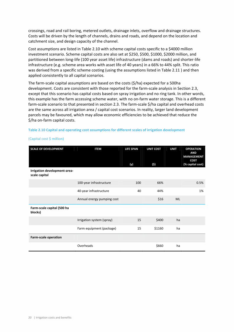
20 | Irrigation costs and benefits
crossings, road and rail boring, metered outlets, drainage inlets, overflow and drainage structures. Costs will be driven by the length of channels, drains and roads, and depend on the location and catchment size, and design capacity of the channel.
Cost assumptions are listed in Table 2.10 with scheme capital costs specific to a $4000 million investment scenario. Scheme capital costs are also set at $250, $500, $1000, $2000 million, and partitioned between long-life (100 year asset life) infrastructure (dams and roads) and shorter-life infrastructure (e.g. scheme area works with asset life of 40 years) in a 66% to 44% split. This ratio was derived from a specific scheme costing (using the assumptions listed in Table 2.11 ) and then applied consistently to all capital scenarios.
The farm-scale capital assumptions are based on the costs ($/ha) expected for a 500ha development. Costs are consistent with those reported for the farm-scale analysis in Section 2.3, except that this scenario has capital costs based on spray irrigation and no ring tank. In other words, this example has the farm accessing scheme water, with no on-farm water storage. This is a different farm-scale scenario to that presented in section 2.3. The farm-scale $/ha capital and overhead costs are the same across all irrigation area / capital cost scenarios. In reality, larger land development parcels may be favoured, which may allow economic efficiencies to be achieved that reduce the $/ha on-farm capital costs.
Table 2.10 Capital and operating cost assumptions for different scales of irrigation development
(Capital cost $ million)
SCALE OF DEVELOPMENT ITEM LIFE SPAN
(y)
UNIT COST
($)
UNIT OPERATION AND
MANAGEMENT COST
(% capital cost)
Irrigation development-area-scale capital
100-year infrastructure 100 66% 0.5%
40-year infrastructure 40 44% 1%
Annual energy pumping cost $16 ML
Farm-scale capital (500 ha blocks)
Irrigation system (spray) 15 $400 ha
Farm equipment (package) 15 $1160 ha
Farm-scale operation
Overheads $660 ha
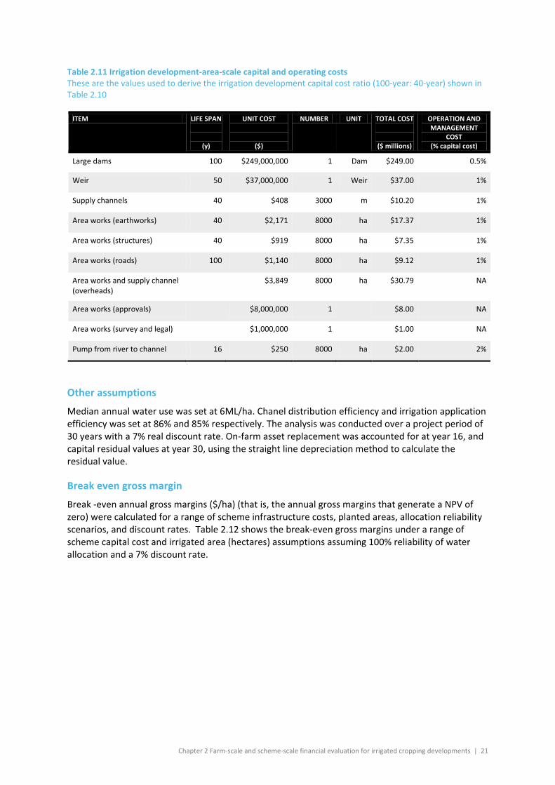
Chapter 2 Farm-scale and scheme-scale financial evaluation for irrigated cropping developments | 21
Table 2.11 Irrigation development-area-scale capital and operating costs These are the values used to derive the irrigation development capital cost ratio (100-year: 40-year) shown in Table 2.10
ITEM LIFE SPAN
(y)
UNIT COST
($)
NUMBER UNIT TOTAL COST
($ millions)
OPERATION AND MANAGEMENT
COST (% capital cost)
Large dams 100 $249,000,000 1 Dam $249.00 0.5%
Weir 50 $37,000,000 1 Weir $37.00 1%
Supply channels 40 $408 3000 m $10.20 1%
Area works (earthworks) 40 $2,171 8000 ha $17.37 1%
Area works (structures) 40 $919 8000 ha $7.35 1%
Area works (roads) 100 $1,140 8000 ha $9.12 1%
Area works and supply channel (overheads)
$3,849 8000 ha $30.79 NA
Area works (approvals) $8,000,000 1 $8.00 NA
Area works (survey and legal) $1,000,000 1 $1.00 NA
Pump from river to channel 16 $250 8000 ha $2.00 2%
Other assumptions
Median annual water use was set at 6ML/ha. Chanel distribution efficiency and irrigation application efficiency was set at 86% and 85% respectively. The analysis was conducted over a project period of 30 years with a 7% real discount rate. On-farm asset replacement was accounted for at year 16, and capital residual values at year 30, using the straight line depreciation method to calculate the residual value.
Break even gross margin
Break -even annual gross margins ($/ha) (that is, the annual gross margins that generate a NPV of zero) were calculated for a range of scheme infrastructure costs, planted areas, allocation reliability scenarios, and discount rates. Table 2.12 shows the break-even gross margins under a range of scheme capital cost and irrigated area (hectares) assumptions assuming 100% reliability of water allocation and a 7% discount rate.
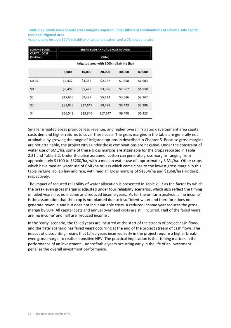
22 | Irrigation costs and benefits
Table 2.12 Break-even annual gross margins required under different combinations of scheme-sale capital cost and irrigated area Assumptions include 100% reliability of water allocation and a 7% discount rate.
SCHEME-SCALE CAPITAL COST ($ billion)
BREAK-EVEN ANNUAL GROSS MARGIN
($/ha)
Irrigated area with 100% reliability (ha)
5,000 10,000 20,000 40,000 80,000
$0.25 $5,422 $3,385 $2,367 $1,858 $1,603
$0.5 $9,497 $5,423 $3,386 $2,367 $1,858
$1 $17,646 $9,497 $5,423 $3,386 $2,367
$2 $33,945 $17,647 $9,498 $5,423 $3,386
$4 $66,543 $33,946 $17,647 $9,498 $5,423
Smaller irrigated areas produce less revenue, and higher overall irrigated development area capital costs demand higher returns to cover these costs. The gross margins in the table are generally not attainable by growing the range of irrigated options in described in Chapter 5. Because gross margins are not attainable, the project NPVs under these combinations are negative. Under the constraint of water use of 6ML/ha, some of these gross margins are attainable for the crops reported in Table 2.21 and Table 2.2. Under the price assumed, cotton can generate gross margins ranging from approximately $1100 to $3200/ha, with a median water use of approximately 3 ML/ha. Other crops which have median water use of 6ML/ha or less which come close to the lowest gross margin in this table include lab lab hay and rice, with median gross margins of $1354/ha and $1368/ha (Flinders), respectively.
The impact of reduced reliability of water allocation is presented in Table 2.13 as the factor by which the break even gross margin is adjusted under four reliability scenarios, which also reflect the timing of failed years (i.e. no income and reduced income years. As for the on-farm analysis, a ‘no income’ is the assumption that the crop is not planted due to insufficient water and therefore does not generate revenue and but does not incur variable costs. A reduced income year reduces the gross margin by 50%. All capital costs and annual overhead costs are still incurred. Half of the failed years are ‘no income’ and half are ‘reduced income’.
In the ‘early’ scenario, the failed years are incurred at the start of the stream of project cash flows, and the ‘late’ scenario has failed years occurring at the end of the project stream of cash flows. The impact of discounting means that failed years incurred early in the project require a higher break-even gross margin to realise a positive NPV. The practical implication is that timing matters in the performance of an investment – unprofitable years occurring early in the life of an investment penalise the overall investment performance.
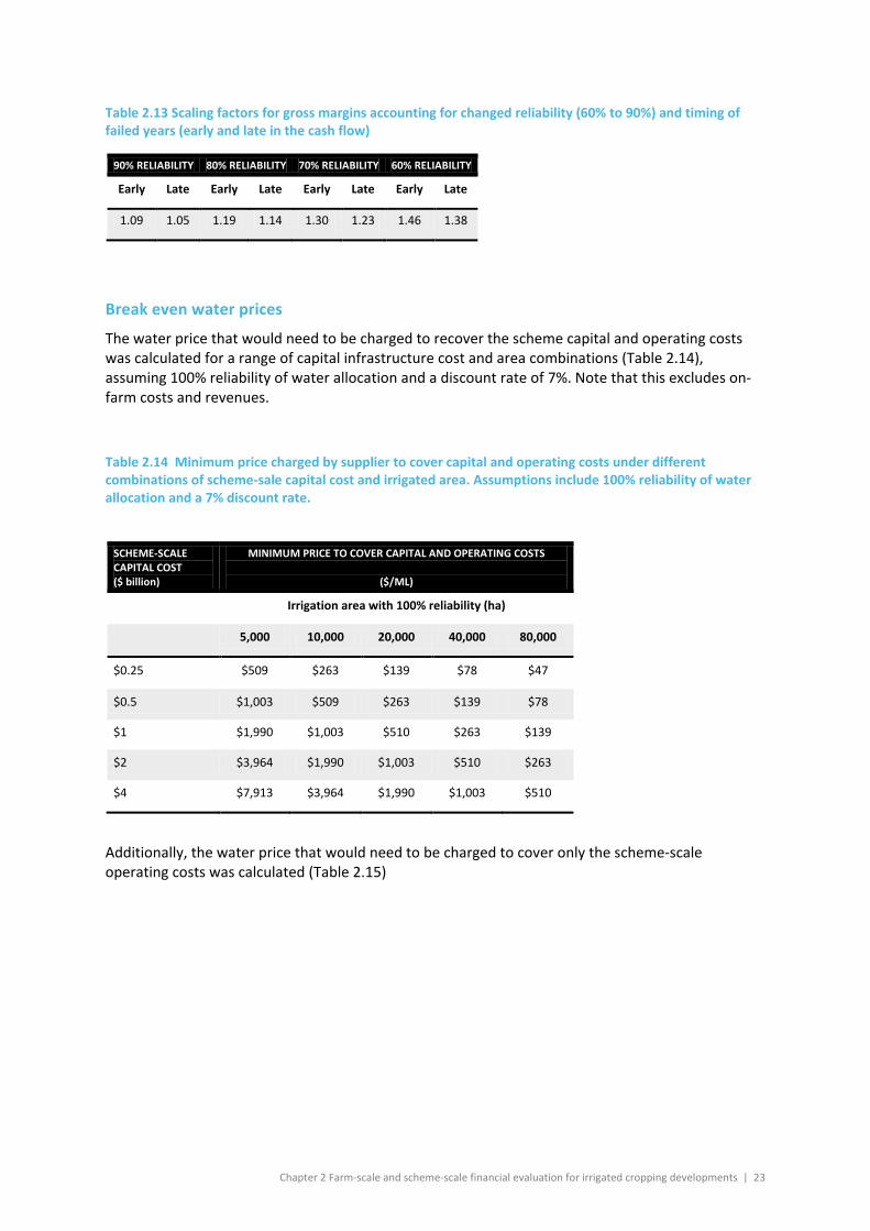
Chapter 2 Farm-scale and scheme-scale financial evaluation for irrigated cropping developments | 23
Table 2.13 Scaling factors for gross margins accounting for changed reliability (60% to 90%) and timing of failed years (early and late in the cash flow)
90% RELIABILITY 80% RELIABILITY 70% RELIABILITY 60% RELIABILITY
Early Late Early Late Early Late Early Late
1.09 1.05 1.19 1.14 1.30 1.23 1.46 1.38
Break even water prices
The water price that would need to be charged to recover the scheme capital and operating costs was calculated for a range of capital infrastructure cost and area combinations (Table 2.14), assuming 100% reliability of water allocation and a discount rate of 7%. Note that this excludes on-farm costs and revenues.
Table 2.14 Minimum price charged by supplier to cover capital and operating costs under different combinations of scheme-sale capital cost and irrigated area. Assumptions include 100% reliability of water allocation and a 7% discount rate.
SCHEME-SCALE CAPITAL COST ($ billion)
MINIMUM PRICE TO COVER CAPITAL AND OPERATING COSTS
($/ML)
Irrigation area with 100% reliability (ha)
5,000 10,000 20,000 40,000 80,000
$0.25 $509 $263 $139 $78 $47
$0.5 $1,003 $509 $263 $139 $78
$1 $1,990 $1,003 $510 $263 $139
$2 $3,964 $1,990 $1,003 $510 $263
$4 $7,913 $3,964 $1,990 $1,003 $510
Additionally, the water price that would need to be charged to cover only the scheme-scale operating costs was calculated (Table 2.15)
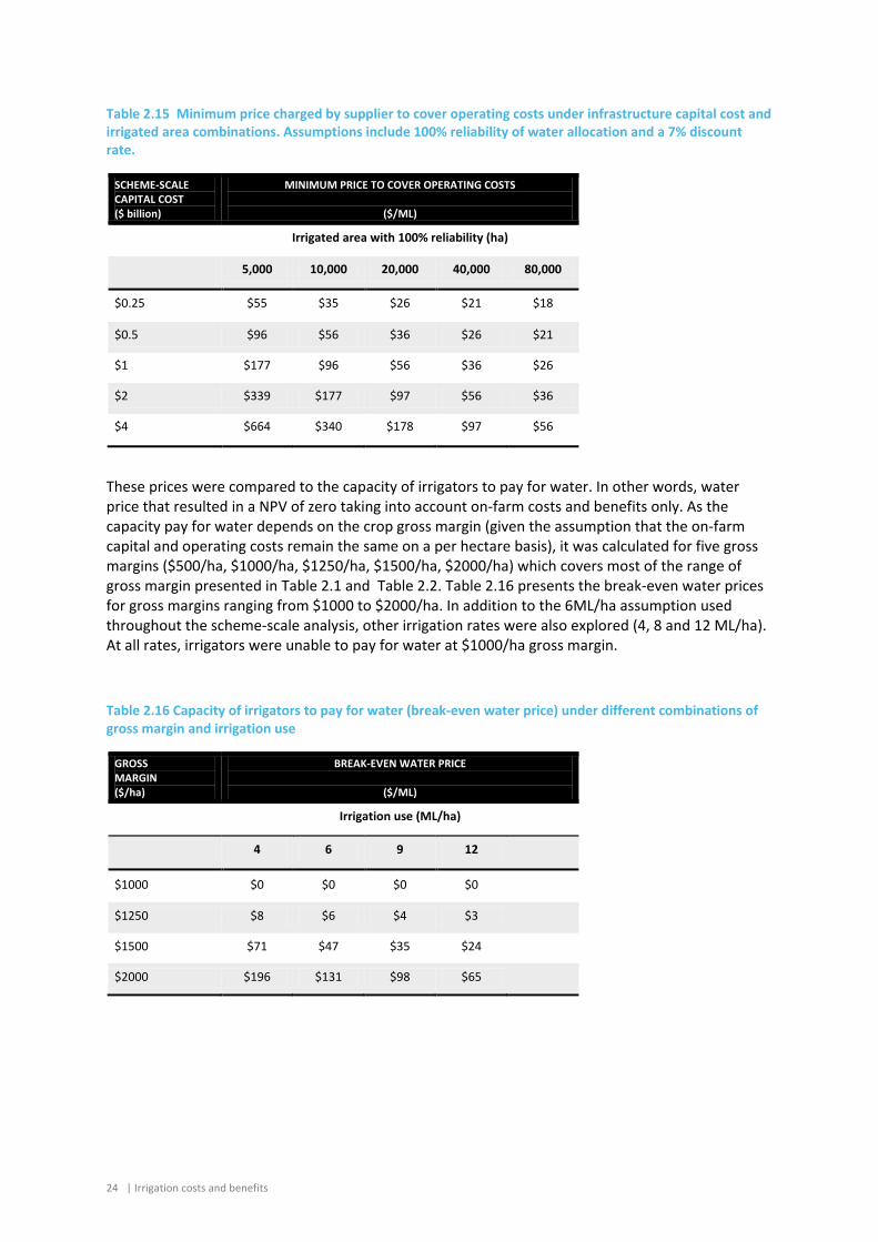
24 | Irrigation costs and benefits
Table 2.15 Minimum price charged by supplier to cover operating costs under infrastructure capital cost and irrigated area combinations. Assumptions include 100% reliability of water allocation and a 7% discount rate.
SCHEME-SCALE CAPITAL COST ($ billion)
MINIMUM PRICE TO COVER OPERATING COSTS
($/ML)
Irrigated area with 100% reliability (ha)
5,000 10,000 20,000 40,000 80,000
$0.25 $55 $35 $26 $21 $18
$0.5 $96 $56 $36 $26 $21
$1 $177 $96 $56 $36 $26
$2 $339 $177 $97 $56 $36
$4 $664 $340 $178 $97 $56
These prices were compared to the capacity of irrigators to pay for water. In other words, water price that resulted in a NPV of zero taking into account on-farm costs and benefits only. As the capacity pay for water depends on the crop gross margin (given the assumption that the on-farm capital and operating costs remain the same on a per hectare basis), it was calculated for five gross margins ($500/ha, $1000/ha, $1250/ha, $1500/ha, $2000/ha) which covers most of the range of gross margin presented in Table 2.1 and Table 2.2. Table 2.16 presents the break-even water prices for gross margins ranging from $1000 to $2000/ha. In addition to the 6ML/ha assumption used throughout the scheme-scale analysis, other irrigation rates were also explored (4, 8 and 12 ML/ha). At all rates, irrigators were unable to pay for water at $1000/ha gross margin.
Table 2.16 Capacity of irrigators to pay for water (break-even water price) under different combinations of gross margin and irrigation use
GROSS MARGIN ($/ha)
BREAK-EVEN WATER PRICE
($/ML)
Irrigation use (ML/ha)
4 6 9 12
$1000 $0 $0 $0 $0
$1250 $8 $6 $4 $3
$1500 $71 $47 $35 $24
$2000 $196 $131 $98 $65
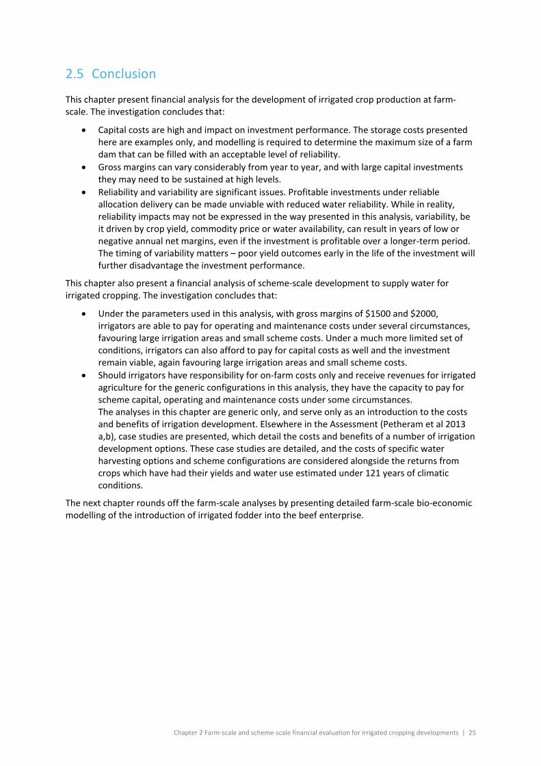
Chapter 2 Farm-scale and scheme-scale financial evaluation for irrigated cropping developments | 25
2.5 Conclusion
This chapter present financial analysis for the development of irrigated crop production at farm-scale. The investigation concludes that:
• Capital costs are high and impact on investment performance. The storage costs presented here are examples only, and modelling is required to determine the maximum size of a farm dam that can be filled with an acceptable level of reliability.
• Gross margins can vary considerably from year to year, and with large capital investments they may need to be sustained at high levels.
• Reliability and variability are significant issues. Profitable investments under reliable allocation delivery can be made unviable with reduced water reliability. While in reality, reliability impacts may not be expressed in the way presented in this analysis, variability, be it driven by crop yield, commodity price or water availability, can result in years of low or negative annual net margins, even if the investment is profitable over a longer-term period. The timing of variability matters – poor yield outcomes early in the life of the investment will further disadvantage the investment performance.
This chapter also present a financial analysis of scheme-scale development to supply water for irrigated cropping. The investigation concludes that:
• Under the parameters used in this analysis, with gross margins of $1500 and $2000, irrigators are able to pay for operating and maintenance costs under several circumstances, favouring large irrigation areas and small scheme costs. Under a much more limited set of conditions, irrigators can also afford to pay for capital costs as well and the investment remain viable, again favouring large irrigation areas and small scheme costs.
• Should irrigators have responsibility for on-farm costs only and receive revenues for irrigated agriculture for the generic configurations in this analysis, they have the capacity to pay for scheme capital, operating and maintenance costs under some circumstances. The analyses in this chapter are generic only, and serve only as an introduction to the costs and benefits of irrigation development. Elsewhere in the Assessment (Petheram et al 2013 a,b), case studies are presented, which detail the costs and benefits of a number of irrigation development options. These case studies are detailed, and the costs of specific water harvesting options and scheme configurations are considered alongside the returns from crops which have had their yields and water use estimated under 121 years of climatic conditions.
The next chapter rounds off the farm-scale analyses by presenting detailed farm-scale bio-economic modelling of the introduction of irrigated fodder into the beef enterprise.
26 | Irrigation costs and benefits
3 Farm-scale evaluation of irrigated fodder production
3.1 Introduction
The dominant agricultural activity in the gulf catchments of north Queensland is breeding beef cattle for slaughter or live export markets, as well as turning off store cattle for fattening on properties outside the region or in feedlots. If more abundant and better quality feed can be produced under irrigation on-property, then producers may be able to attain higher prices per animal, and potentially access different markets, via a combination of shorter or longer fattening periods (by either getting the weight on more quickly or turning off stock at an older, but heavier, age) and increased live weight gains of their cattle. In addition, the possibility of reduced costs of procuring supplementary fodder, improved long-term viability of the operation, and more efficient use of the existing property infrastructure through year-round feed supply and more stable herd structures will likely benefit individual cattle operations and the northern beef industry.
The prospect of an irrigation development in the north Queensland gulf catchments area could strengthen the northern Australia beef industry by complementing the production of beef cattle, predominantly from extensive dryland grazing, with irrigated forage grown on the property. This chapter provides a detailed investigation of the property-scale impacts of integrating forage crops into existing beef cattle production operations in the Gilbert and the Flinders catchments, as graze or hay feed, for breeding or fattening of cattle on the properties. Cattle are usually turned off as store cattle to properties elsewhere for finishing for slaughter or growing out for sale in live export markets. Irrigation is expected to enable producers to turn off different types of animals with the aim of fetching higher prices per head and enabling potential access to different markets.
A bio-economic simulation model has been used to assess the production and financial impacts of incorporating irrigation into beef production systems in the Flinders and Gilbert catchments. The model operates at the scale of a single enterprise. A representative property assumed to be located near Richmond provided the basis for the Flinders catchment analysis, and a representative property assumed to be located near Georgetown provided the basis for the Gilbert catchment analysis.
Ultimately, the existing beef cattle operations of the Gilbert and Flinders catchments will only benefit from irrigation if they can make a profit despite very significant capital costs of irrigation investment. Other considerations impacting on investment performance include the adequacy of regional infrastructure, labour availability and risks such as price variability and water reliability. This analysis investigates some of the key conditions under which beef producers may benefit, or not, from an irrigation development at the property scale.
3.2 Methods
3.2.1 REGIONAL BEEF PRODUCTION SYSTEMS
Soil types
Holdings in both Georgetown and Richmond span a mix of sandy granite, clay, and duplex soils. Irrigable alluvial vertisols make up a smaller area of the properties. The main soil types of the Gilbert
Chapter 3 Farm-scale evaluation of irrigated fodder production | 27
and Flinders catchments are described in more detail in the companion technical report of the soil mapping and land suitability activities (Bartley et al., 2013).
Land use and labour
Beef cattle grazing is the primary land use in the Gilbert and Flinders catchments. On average, 92% of the available grazing area is comprised of native pastures (Gleeson et al., 2012), with limited sown or improved pastures (e.g. sown grasses or over-sown legumes).
The labour force on most northern properties is typically 1 to 3 full-time equivalent positions of fixed and casual labour, with additional labour required in the dry season to help with supplementary feeding of livestock, as well as undertaking animal husbandry and farm maintenance work.
Beef production systems
The dominant beef production system that is employed across most of northern Australia is centred on a cow-calf breeding operation with several variations in the post-weaning management and marketing of male animals produced by the breeding herds (Gleeson et al., 2012). Some enterprises specialise in breeding and turning off very young stock after weaning (six to nine months), some retain and grow young animals to weights that are suited for the live export trade (300 to 350 kg at 12 to 18 months), and others carry older steers through to heavier weights suited to feedlot finishing (360 to 450 kg at 24 months) or slaughter for north Asian markets (560 to 620 kg at 30 to 40 months). The final choice for any single holding is largely determined through the interplay of land resource endowments, local climate and market opportunities. In many instances, these variants of the cow-calf breeding system are conducted across geographically segregated holdings that are integrated under common ownership and management.
Breeding systems in the Gilbert catchment
Most of these production system variants, including the geographic separation of system components, are found on beef holdings located in the Gilbert River catchment; although cow-calf breeding systems that turn off weaners of both sexes, and light steers for export or backgrounding, are the more common. Beef cattle holdings in the region that are an integral component of geographically segregated production enterprises will generally run a specialist breeder herd and transfer young and often newly weaned animals of both sexes to other holdings outside the region for growing out for live export, backgrounding for feedlots or finishing for slaughter. While many holdings retain a proportion of their own-bred heifers to maintain breeding herd numbers after culling or mortalities, others source their replacement breeders from other regions where they have already been grown out to a suitable weight and condition for mating. If suitable conditions prevail, and especially if forage supplies are adequate, many holdings may finish cull breeders and older steers to heavier weight classes for slaughter.
The forage base for cattle enterprises in the Gilbert region is largely comprised of unimproved native pastures with only limited areas of sown grasses and legumes. These pastures generally provide a plentiful supply of herbage for grazing in the wet season, although there is considerable year to year variation in the total quantity and quality of available pasture due to seasonal rainfall variability. Herbage quality declines rapidly with the onset of the annual dry season during which feed shortages are also prevalent. As a result, annual animal growth patterns typically follow a sequence of seasonal weight gains and weight losses which impact on the ability of stock to reach different market weight for age specifications, as well as impact on the reproductive performance of breeders. Dry season feeding of energy and protein enriched supplements (e.g. urea and molasses; cotton seed meal) to some or all stock classes is commonly practiced. Some enterprises also feed hay to stock, especially in very dry seasons (Gleeson et al., 2012), and this may be produced locally
28 | Irrigation costs and benefits
by cutting and baling dryland pastures or limited irrigation of sown pasture or trucked in from other regions (e.g. sub-coastal regions, Atherton Tablelands).
Stocking rates on native and semi-natural pastures in the Gilbert region vary considerably according to land and vegetation types, prevailing seasonal conditions, and management. However, stocking rates are generally more conservative than those applied in more favourable temperate regions (e.g. southern Australia) and a long-term average of approximately one adult equivalent (AE1) per 15 to 20 ha might represent a sustainable stocking rate for much of the Flinders region (B. English, pers. comm.).
Reproductive efficiency of northern Australian beef herds varies considerably and low weaning rates, especially from Bos indicus dominant herds, remains a significant source of economic loss (McCosker et al., 2010). Two particular management challenges that are directly influenced by diet include growing out young heifers to sufficient size and weight for a successful first mating and returning first calf breeders back to a suitable physiological condition to sustain a second pregnancy within a 12-month mating cycle (Schatz, 2012).
Fattening systems in the Flinders catchment
The geographic separation of production system components applies to many of the beef holdings that are located in the Flinders catchment. Relatively few of these holdings carry significant breeding herds - rather, they typically receive young and often newly weaned animals of both sexes from large specialist breeding operations located outside the Flinders catchment (e.g. Barkly Tableland, Cape York or elsewhere in north-west Queensland) for growing out or finishing for slaughter.
As is the case for the Gilbert catchment, the forage base for cattle enterprises in the Flinders catchment is also largely comprised of unimproved native pastures with limited areas of sown grasses and legumes. Pasture and animal growth patterns are also similar with a plentiful supply of wet season herbage and considerable year to year variation in forage availability and quality with resulting annual animal growth patterns characterised by sequential seasonal weight gains and weight losses. Dry season feeding of energy and protein enriched supplements to some or all stock classes is commonly practised, and some enterprises also feed hay to stock, especially in very dry seasons (Gleeson et al., 2012). This may be produced locally by cutting and baling dryland pastures or sown pasture with limited irrigation or it may be trucked in from other regions (e.g. sub-coastal regions or the Central Highlands).
Although factors such as genetic makeup, physiological state, health, ambient temperature, stress, distance to water and general husbandry have an impact on beef reproductive efficiency and animal growth and, a key driver remains the unrestricted availability and intake of digestible dry matter. It is in this regard that the opportunities for irrigation to directly impact on the productivity and profitability of existing beef enterprises in the Gilbert and Flinders catchments are best considered.
Growth patterns of beef cattle in northern Australia
The prospective markets that can be accessed for a particular class of cattle in a herd (e.g. weaner steers, three-year old bullocks, cull breeding cows etc.) are largely determined by the pattern of growth of those animals relative to their age, and this is significantly influenced by the type of pastures on which they are grazed and the extent to which high quality forages and grain might be employed to supplement their diet. The capacity of different types of pastures, forage crops and grain to produce live weight gain in beef cattle is well understood and most beef enterprises will use that knowledge against their available pasture resources to develop feeding regimes to produce
1 Adult equivalent is the grazing pressure exerted by a non-pregnant, non-lactating breeding cow of 455 kg live weight
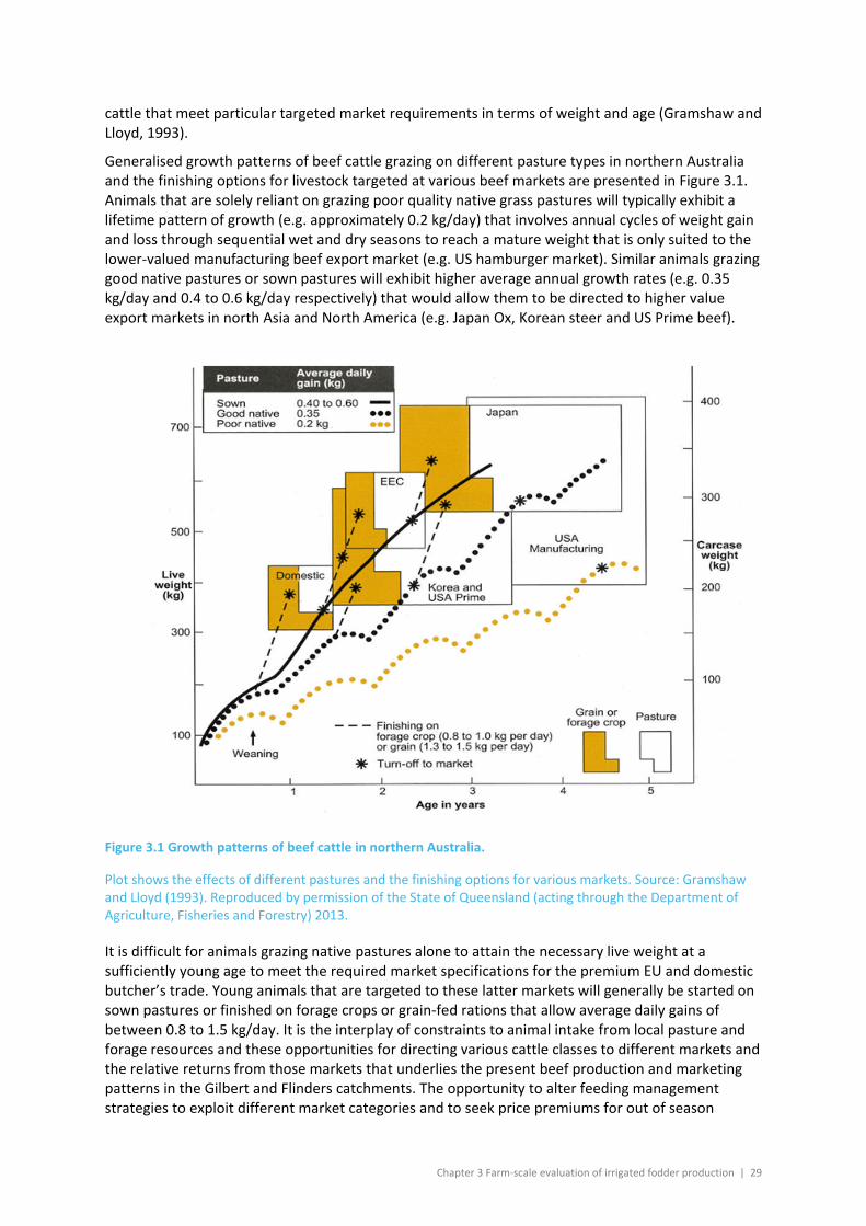
Chapter 3 Farm-scale evaluation of irrigated fodder production | 29
cattle that meet particular targeted market requirements in terms of weight and age (Gramshaw and Lloyd, 1993).
Generalised growth patterns of beef cattle grazing on different pasture types in northern Australia and the finishing options for livestock targeted at various beef markets are presented in Figure 3.1. Animals that are solely reliant on grazing poor quality native grass pastures will typically exhibit a lifetime pattern of growth (e.g. approximately 0.2 kg/day) that involves annual cycles of weight gain and loss through sequential wet and dry seasons to reach a mature weight that is only suited to the lower-valued manufacturing beef export market (e.g. US hamburger market). Similar animals grazing good native pastures or sown pastures will exhibit higher average annual growth rates (e.g. 0.35 kg/day and 0.4 to 0.6 kg/day respectively) that would allow them to be directed to higher value export markets in north Asia and North America (e.g. Japan Ox, Korean steer and US Prime beef).
Figure 3.1 Growth patterns of beef cattle in northern Australia.
Plot shows the effects of different pastures and the finishing options for various markets. Source: Gramshaw and Lloyd (1993). Reproduced by permission of the State of Queensland (acting through the Department of Agriculture, Fisheries and Forestry) 2013.
It is difficult for animals grazing native pastures alone to attain the necessary live weight at a sufficiently young age to meet the required market specifications for the premium EU and domestic butcher’s trade. Young animals that are targeted to these latter markets will generally be started on sown pastures or finished on forage crops or grain-fed rations that allow average daily gains of between 0.8 to 1.5 kg/day. It is the interplay of constraints to animal intake from local pasture and forage resources and these opportunities for directing various cattle classes to different markets and the relative returns from those markets that underlies the present beef production and marketing patterns in the Gilbert and Flinders catchments. The opportunity to alter feeding management strategies to exploit different market categories and to seek price premiums for out of season
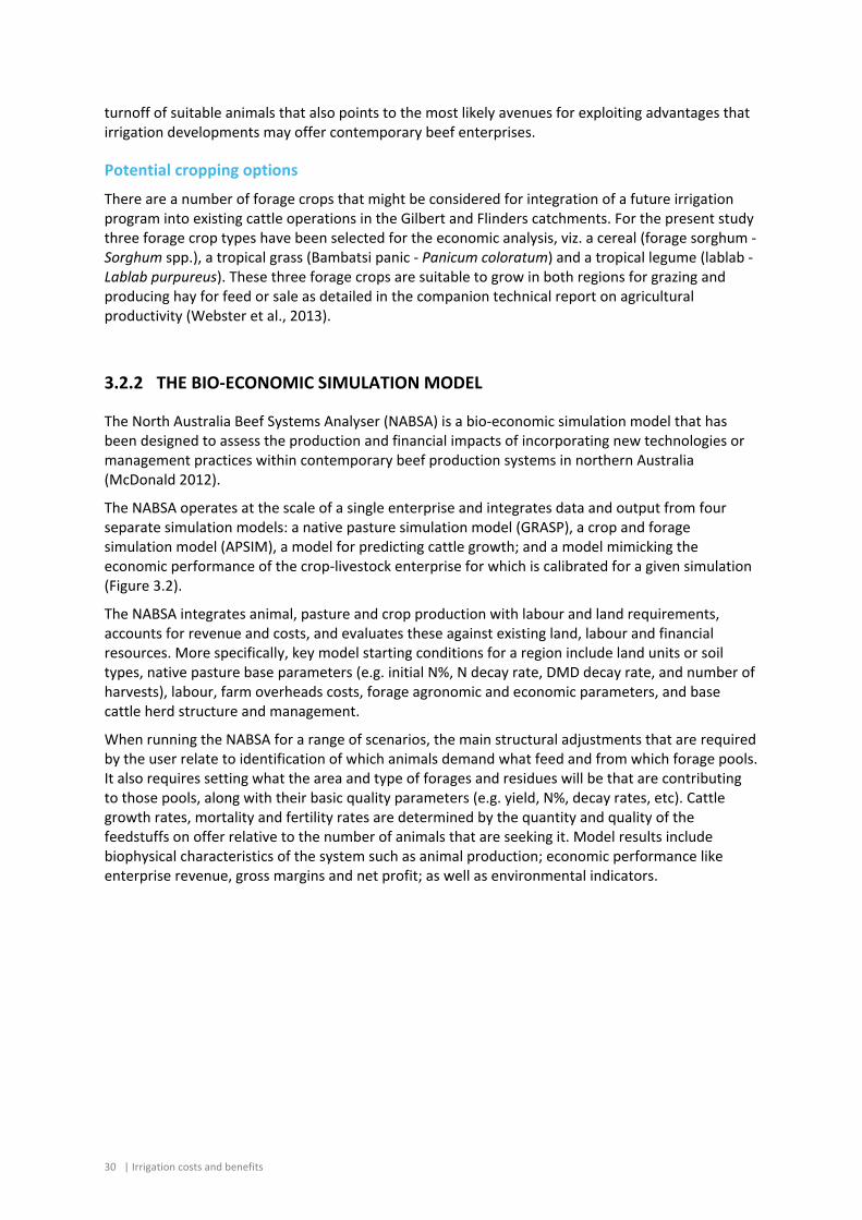
30 | Irrigation costs and benefits
turnoff of suitable animals that also points to the most likely avenues for exploiting advantages that irrigation developments may offer contemporary beef enterprises.
Potential cropping options
There are a number of forage crops that might be considered for integration of a future irrigation program into existing cattle operations in the Gilbert and Flinders catchments. For the present study three forage crop types have been selected for the economic analysis, viz. a cereal (forage sorghum - Sorghum spp.), a tropical grass (Bambatsi panic - Panicum coloratum) and a tropical legume (lablab - Lablab purpureus). These three forage crops are suitable to grow in both regions for grazing and producing hay for feed or sale as detailed in the companion technical report on agricultural productivity (Webster et al., 2013).
3.2.2 THE BIO-ECONOMIC SIMULATION MODEL
The North Australia Beef Systems Analyser (NABSA) is a bio-economic simulation model that has been designed to assess the production and financial impacts of incorporating new technologies or management practices within contemporary beef production systems in northern Australia (McDonald 2012).
The NABSA operates at the scale of a single enterprise and integrates data and output from four separate simulation models: a native pasture simulation model (GRASP), a crop and forage simulation model (APSIM), a model for predicting cattle growth; and a model mimicking the economic performance of the crop-livestock enterprise for which is calibrated for a given simulation (Figure 3.2).
The NABSA integrates animal, pasture and crop production with labour and land requirements, accounts for revenue and costs, and evaluates these against existing land, labour and financial resources. More specifically, key model starting conditions for a region include land units or soil types, native pasture base parameters (e.g. initial N%, N decay rate, DMD decay rate, and number of harvests), labour, farm overheads costs, forage agronomic and economic parameters, and base cattle herd structure and management.
When running the NABSA for a range of scenarios, the main structural adjustments that are required by the user relate to identification of which animals demand what feed and from which forage pools. It also requires setting what the area and type of forages and residues will be that are contributing to those pools, along with their basic quality parameters (e.g. yield, N%, decay rates, etc). Cattle growth rates, mortality and fertility rates are determined by the quantity and quality of the feedstuffs on offer relative to the number of animals that are seeking it. Model results include biophysical characteristics of the system such as animal production; economic performance like enterprise revenue, gross margins and net profit; as well as environmental indicators.
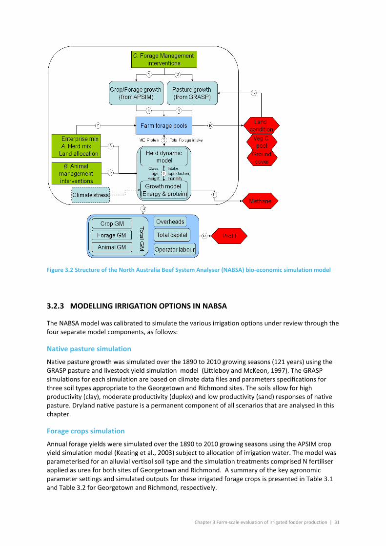
Chapter 3 Farm-scale evaluation of irrigated fodder production | 31
Figure 3.2 Structure of the North Australia Beef System Analyser (NABSA) bio-economic simulation model
3.2.3 MODELLING IRRIGATION OPTIONS IN NABSA
The NABSA model was calibrated to simulate the various irrigation options under review through the four separate model components, as follows:
Native pasture simulation
Native pasture growth was simulated over the 1890 to 2010 growing seasons (121 years) using the GRASP pasture and livestock yield simulation model (Littleboy and McKeon, 1997). The GRASP simulations for each simulation are based on climate data files and parameters specifications for three soil types appropriate to the Georgetown and Richmond sites. The soils allow for high productivity (clay), moderate productivity (duplex) and low productivity (sand) responses of native pasture. Dryland native pasture is a permanent component of all scenarios that are analysed in this chapter.
Forage crops simulation
Annual forage yields were simulated over the 1890 to 2010 growing seasons using the APSIM crop yield simulation model (Keating et al., 2003) subject to allocation of irrigation water. The model was parameterised for an alluvial vertisol soil type and the simulation treatments comprised N fertiliser applied as urea for both sites of Georgetown and Richmond. A summary of the key agronomic parameter settings and simulated outputs for these irrigated forage crops is presented in Table 3.1 and Table 3.2 for Georgetown and Richmond, respectively.
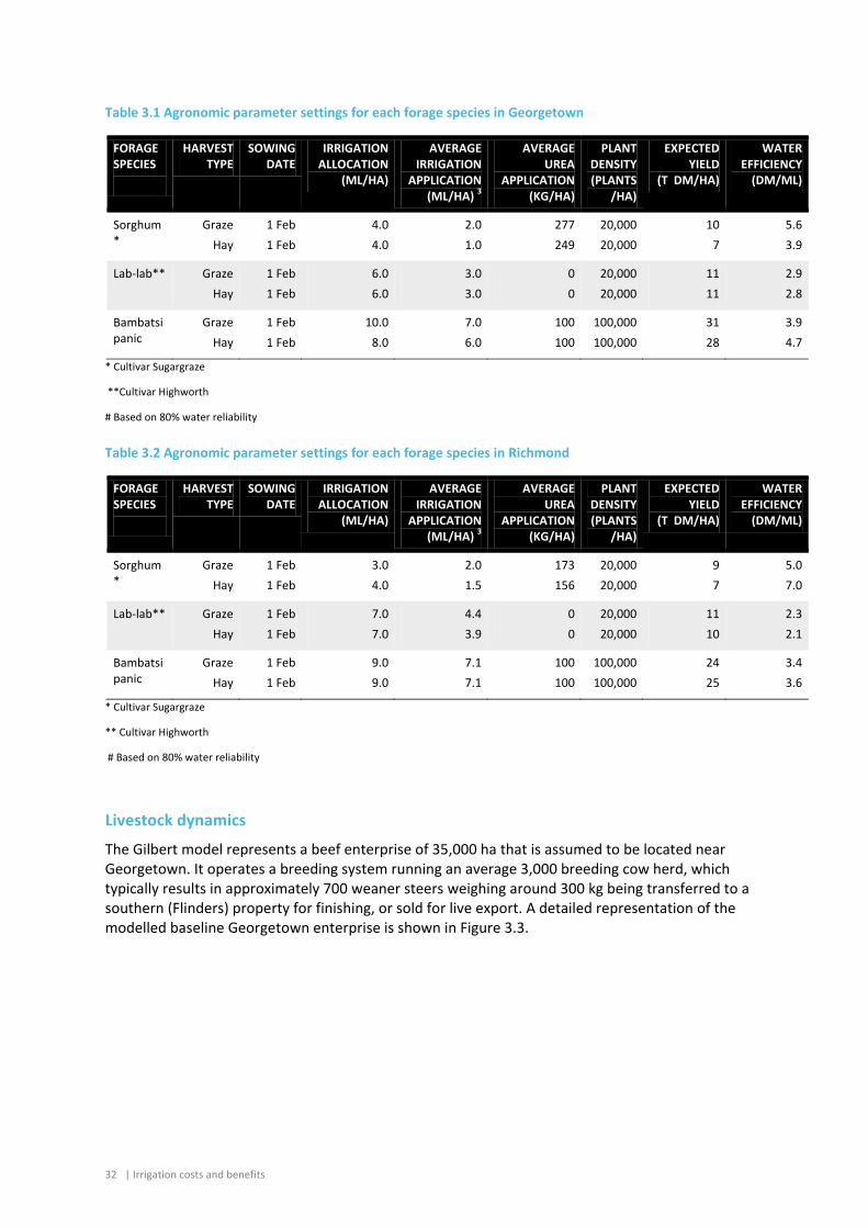
32 | Irrigation costs and benefits
Table 3.1 Agronomic parameter settings for each forage species in Georgetown
FORAGE SPECIES
HARVEST TYPE
SOWING DATE
IRRIGATION ALLOCATION
(ML/HA)
AVERAGE IRRIGATION
APPLICATION (ML/HA) 3
AVERAGE UREA
APPLICATION (KG/HA)
PLANT DENSITY (PLANTS
/HA)
EXPECTED YIELD
(T DM/HA)
WATER EFFICIENCY
(DM/ML)
Sorghum*
Graze Hay
1 Feb 1 Feb
4.0 4.0
2.0 1.0
277 249
20,000 20,000
10 7
5.6 3.9
Lab-lab** Graze Hay
1 Feb 1 Feb
6.0 6.0
3.0 3.0
0 0
20,000 20,000
11 11
2.9 2.8
Bambatsi panic
Graze Hay
1 Feb 1 Feb
10.0 8.0
7.0 6.0
100 100
100,000 100,000
31 28
3.9 4.7
* Cultivar Sugargraze
**Cultivar Highworth
# Based on 80% water reliability
Table 3.2 Agronomic parameter settings for each forage species in Richmond
FORAGE SPECIES
HARVEST TYPE
SOWING DATE
IRRIGATION ALLOCATION
(ML/HA)
AVERAGE IRRIGATION
APPLICATION (ML/HA) 3
AVERAGE UREA
APPLICATION (KG/HA)
PLANT DENSITY (PLANTS
/HA)
EXPECTED YIELD
(T DM/HA)
WATER EFFICIENCY
(DM/ML)
Sorghum*
Graze Hay
1 Feb 1 Feb
3.0 4.0
2.0 1.5
173 156
20,000 20,000
9 7
5.0 7.0
Lab-lab** Graze Hay
1 Feb 1 Feb
7.0 7.0
4.4 3.9
0 0
20,000 20,000
11 10
2.3 2.1
Bambatsi panic
Graze Hay
1 Feb 1 Feb
9.0 9.0
7.1 7.1
100 100
100,000 100,000
24 25
3.4 3.6
* Cultivar Sugargraze
** Cultivar Highworth
# Based on 80% water reliability
Livestock dynamics
The Gilbert model represents a beef enterprise of 35,000 ha that is assumed to be located near Georgetown. It operates a breeding system running an average 3,000 breeding cow herd, which typically results in approximately 700 weaner steers weighing around 300 kg being transferred to a southern (Flinders) property for finishing, or sold for live export. A detailed representation of the modelled baseline Georgetown enterprise is shown in Figure 3.3.
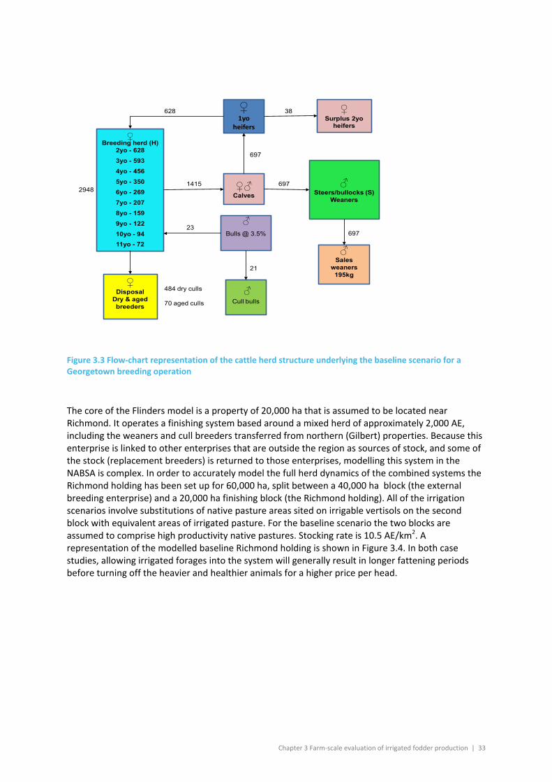
Chapter 3 Farm-scale evaluation of irrigated fodder production | 33
Breeding herd (H)2yo - 6283yo - 5934yo - 4565yo - 3506yo - 2697yo - 2078yo - 1599yo - 122 10yo - 9411yo - 72
♂Steers/bullocks (S)
Weaners
♀♂Calves
♀1yo
heifers
♀Surplus 2yo
heifers
♀Disposal
Dry & aged breeders
♂Sales
weaners195kg
♀
2948
628
697
38
1415
484 dry culls
70 aged culls
697
697Bulls @ 3.5%
♂
Cull bulls♂
23
21
Figure 3.3 Flow-chart representation of the cattle herd structure underlying the baseline scenario for a Georgetown breeding operation
The core of the Flinders model is a property of 20,000 ha that is assumed to be located near Richmond. It operates a finishing system based around a mixed herd of approximately 2,000 AE, including the weaners and cull breeders transferred from northern (Gilbert) properties. Because this enterprise is linked to other enterprises that are outside the region as sources of stock, and some of the stock (replacement breeders) is returned to those enterprises, modelling this system in the NABSA is complex. In order to accurately model the full herd dynamics of the combined systems the Richmond holding has been set up for 60,000 ha, split between a 40,000 ha block (the external breeding enterprise) and a 20,000 ha finishing block (the Richmond holding). All of the irrigation scenarios involve substitutions of native pasture areas sited on irrigable vertisols on the second block with equivalent areas of irrigated pasture. For the baseline scenario the two blocks are assumed to comprise high productivity native pastures. Stocking rate is 10.5 AE/km2. A representation of the modelled baseline Richmond holding is shown in Figure 3.4. In both case studies, allowing irrigated forages into the system will generally result in longer fattening periods before turning off the heavier and healthier animals for a higher price per head.
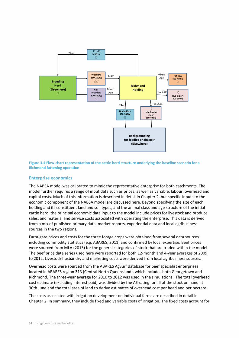
34 | Irrigation costs and benefits
Breeding Herd
(Elsewhere)♀
Weaners180-200kg♀♂
1st calf heifers♀
♂Live export 300-350kg
Cull Breeders
320-350kg♀
Fat cow450-480kg
♀
12-18m
6-8m
24m
Mixed Age
Mixed Age
Richmond Holding
Backgroundingfor feedlot or abattoir
(Elsewhere)
Dry heifers350-360kg
♀
♂Light feedlot
steer 360-400kg
24m 18-20m
Figure 3.4 Flow-chart representation of the cattle herd structure underlying the baseline scenario for a Richmond fattening operation
Enterprise economics
The NABSA model was calibrated to mimic the representative enterprise for both catchments. The model further requires a range of input data such as prices, as well as variable, labour, overhead and capital costs. Much of this information is described in detail in Chapter 2, but specific inputs to the economic component of the NABSA model are discussed here. Beyond specifying the size of each holding and its constituent land and soil types, and the animal class and age structure of the initial cattle herd, the principal economic data input to the model include prices for livestock and produce sales, and material and service costs associated with operating the enterprise. This data is derived from a mix of published primary data, market reports, experiential data and local agribusiness sources in the two regions.
Farm-gate prices and costs for the three forage crops were obtained from several data sources including commodity statistics (e.g. ABARES, 2011) and confirmed by local expertise. Beef prices were sourced from MLA (2013) for the general categories of stock that are traded within the model. The beef price data series used here were reported for both 12-month and 4-year averages of 2009 to 2012. Livestock husbandry and marketing costs were derived from local agribusiness sources.
Overhead costs were sourced from the ABARES AgSurf database for beef specialist enterprises located in ABARES region 313 (Central North Queensland), which includes both Georgetown and Richmond. The three-year average for 2010 to 2012 was used in the simulations. The total overhead cost estimate (excluding interest paid) was divided by the AE rating for all of the stock on hand at 30th June and the total area of land to derive estimates of overhead cost per head and per hectare.
The costs associated with irrigation development on individual farms are described in detail in Chapter 2. In summary, they include fixed and variable costs of irrigation. The fixed costs account for
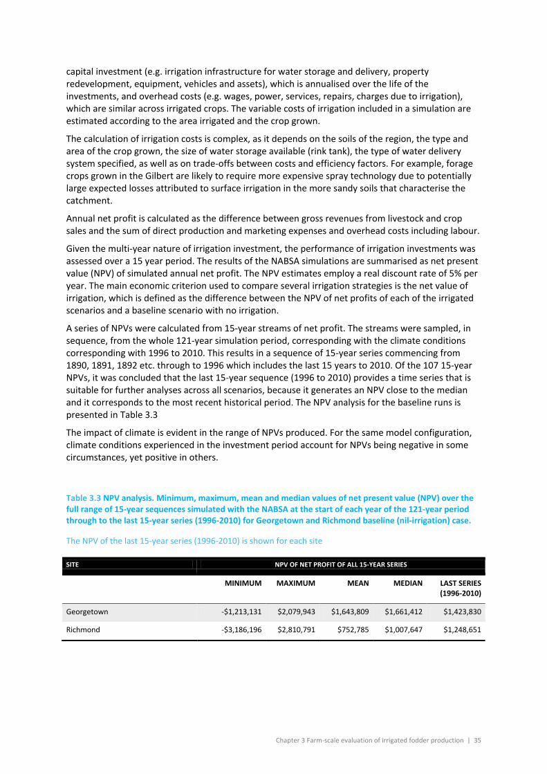
Chapter 3 Farm-scale evaluation of irrigated fodder production | 35
capital investment (e.g. irrigation infrastructure for water storage and delivery, property redevelopment, equipment, vehicles and assets), which is annualised over the life of the investments, and overhead costs (e.g. wages, power, services, repairs, charges due to irrigation), which are similar across irrigated crops. The variable costs of irrigation included in a simulation are estimated according to the area irrigated and the crop grown.
The calculation of irrigation costs is complex, as it depends on the soils of the region, the type and area of the crop grown, the size of water storage available (rink tank), the type of water delivery system specified, as well as on trade-offs between costs and efficiency factors. For example, forage crops grown in the Gilbert are likely to require more expensive spray technology due to potentially large expected losses attributed to surface irrigation in the more sandy soils that characterise the catchment.
Annual net profit is calculated as the difference between gross revenues from livestock and crop sales and the sum of direct production and marketing expenses and overhead costs including labour.
Given the multi-year nature of irrigation investment, the performance of irrigation investments was assessed over a 15 year period. The results of the NABSA simulations are summarised as net present value (NPV) of simulated annual net profit. The NPV estimates employ a real discount rate of 5% per year. The main economic criterion used to compare several irrigation strategies is the net value of irrigation, which is defined as the difference between the NPV of net profits of each of the irrigated scenarios and a baseline scenario with no irrigation.
A series of NPVs were calculated from 15-year streams of net profit. The streams were sampled, in sequence, from the whole 121-year simulation period, corresponding with the climate conditions corresponding with 1996 to 2010. This results in a sequence of 15-year series commencing from 1890, 1891, 1892 etc. through to 1996 which includes the last 15 years to 2010. Of the 107 15-year NPVs, it was concluded that the last 15-year sequence (1996 to 2010) provides a time series that is suitable for further analyses across all scenarios, because it generates an NPV close to the median and it corresponds to the most recent historical period. The NPV analysis for the baseline runs is presented in Table 3.3
The impact of climate is evident in the range of NPVs produced. For the same model configuration, climate conditions experienced in the investment period account for NPVs being negative in some circumstances, yet positive in others.
Table 3.3 NPV analysis. Minimum, maximum, mean and median values of net present value (NPV) over the full range of 15-year sequences simulated with the NABSA at the start of each year of the 121-year period through to the last 15-year series (1996-2010) for Georgetown and Richmond baseline (nil-irrigation) case.
The NPV of the last 15-year series (1996-2010) is shown for each site
SITE NPV OF NET PROFIT OF ALL 15-YEAR SERIES
MINIMUM MAXIMUM MEAN MEDIAN LAST SERIES (1996-2010)
Georgetown -$1,213,131 $2,079,943 $1,643,809 $1,661,412 $1,423,830
Richmond -$3,186,196 $2,810,791 $752,785 $1,007,647 $1,248,651
36 | Irrigation costs and benefits
3.2.4 ANALYSIS DESIGN
The NABSA bio-economic model was used in this study to evaluate the impact of integrating irrigated forage crops within the representative beef enterprise (baseline scenario) for both Georgetown and Richmond. The initial assessment of the net economic benefits attributable to the irrigation options assumes that the net value of irrigated forage estimated for each scenario results from the difference between the average net profit over the 121-year period of that irrigated scenario and the long-term average net profit of the baseline scenario. A series of sensitivity tests and multi-factorial analyses are subsequently applied to the simulation results.
Scenarios
For both the Richmond and Georgetown representative enterprises a comparison is made between five scenarios as follows:
• Scenario 1: cattle only (baseline) • Scenario 2: cattle and 100 ha irrigated forage sorghum for grazing in situ • Scenario 3: cattle and 200 ha irrigated Bambatsi panic for grazing in situ • Scenario 4: cattle and 500 ha irrigated lablab cut for hay (fed back to animals or sale) • Scenario 5: cattle and 1000 ha irrigated forage sorghum cut for hay (fed back to animals or sale)
Developed areas ranging between 100 and 1000 ha were assumed to offer a realistic range for irrigation development in both catchments, along with the three forage types selected as suitable for irrigation (section 3.2.1). Note that the scenarios described here are independent from analyses presented in other chapters of the report. Each scenario is underlined by a different set of assumptions (Table 3.4 and Table 3.5), including forage crop type and area, water demand per crop, irrigation system used, irrigation efficiencies (storage, conveyance and application), storage size and cost, available feed options, access to the feed base, and key livestock changes in selling age, weight and timing, as well as price changes for quality. The storage sizes that have been considered for the scenarios are assumed to hold sufficient to water to meet the demands of the crop, while realistically giving producers flexibility to explore future options of different forages (or other crops) in different years.
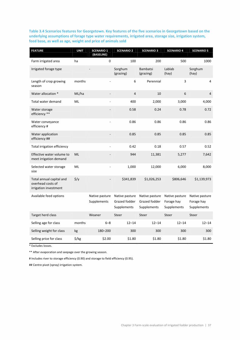
Chapter 3 Farm-scale evaluation of irrigated fodder production | 37
Table 3.4 Scenarios features for Georgetown. Key features of the five scenarios in Georgetown based on the underlying assumptions of forage type water requirements, irrigated area, storage size, irrigation system, feed base, as well as age, weight and price of animals sold
FEATURE UNIT SCENARIO 1 (BASELINE)
SCENARIO 2 SCENARIO 3 SCENARIO 4 SCENARIO 5
Farm irrigated area ha 0 100 200 500 1000
Irrigated forage type - Sorghum (grazing)
Bambatsi (grazing)
Lablab (hay)
Sorghum (hay)
Length of crop growing season
months - 6 Perennial 3 4
Water allocation * ML/ha - 4 10 6 4
Total water demand ML - 400 2,000 3,000 4,000
Water storage efficiency **
- 0.58 0.24 0.78 0.72
Water conveyance efficiency #
- 0.86 0.86 0.86 0.86
Water application efficiency ##
- 0.85 0.85 0.85 0.85
Total irrigation efficiency - 0.42 0.18 0.57 0.52
Effective water volume to meet irrigation demand
ML - 944 11,381 5,277 7,642
Selected water storage size
ML - 1,000 12,000 6,000 8,000
Total annual capital and overhead costs of irrigation investment
$/y - $341,839 $1,026,253 $806,646 $1,139,973
Available feed options Native pasture Supplements
Native pasture Grazed fodder Supplements
Native pasture Grazed fodder Supplements
Native pasture Forage hay Supplements
Native pasture Forage hay Supplements
Target herd class Weaner Steer Steer Steer Steer
Selling age for class months 6–8 12–14 12–14 12–14 12–14
Selling weight for class kg 180–200 300 300 300 300
Selling price for class $/kg $2.00 $1.80 $1.80 $1.80 $1.80
* Excludes losses.
** After evaporation and seepage over the growing season.
# Includes river to storage efficiency (0.90) and storage to field efficiency (0.95).
## Centre pivot (spray) irrigation system.
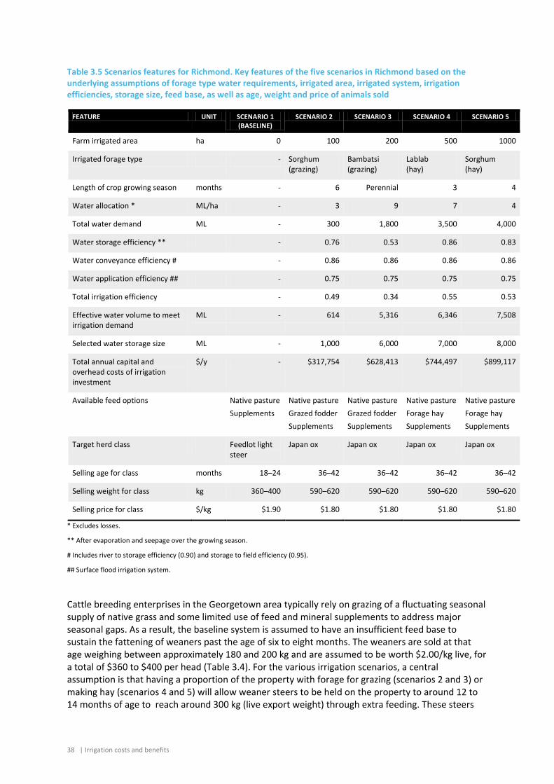
38 | Irrigation costs and benefits
Table 3.5 Scenarios features for Richmond. Key features of the five scenarios in Richmond based on the underlying assumptions of forage type water requirements, irrigated area, irrigated system, irrigation efficiencies, storage size, feed base, as well as age, weight and price of animals sold
FEATURE UNIT SCENARIO 1 (BASELINE)
SCENARIO 2 SCENARIO 3 SCENARIO 4 SCENARIO 5
Farm irrigated area ha 0 100 200 500 1000
Irrigated forage type - Sorghum (grazing)
Bambatsi (grazing)
Lablab (hay)
Sorghum (hay)
Length of crop growing season months - 6 Perennial 3 4
Water allocation * ML/ha - 3 9 7 4
Total water demand ML - 300 1,800 3,500 4,000
Water storage efficiency ** - 0.76 0.53 0.86 0.83
Water conveyance efficiency # - 0.86 0.86 0.86 0.86
Water application efficiency ## - 0.75 0.75 0.75 0.75
Total irrigation efficiency - 0.49 0.34 0.55 0.53
Effective water volume to meet irrigation demand
ML - 614 5,316 6,346 7,508
Selected water storage size ML - 1,000 6,000 7,000 8,000
Total annual capital and overhead costs of irrigation investment
$/y - $317,754 $628,413 $744,497 $899,117
Available feed options Native pasture Supplements
Native pasture Grazed fodder Supplements
Native pasture Grazed fodder Supplements
Native pasture Forage hay Supplements
Native pasture Forage hay Supplements
Target herd class Feedlot light steer
Japan ox Japan ox Japan ox Japan ox
Selling age for class months 18–24 36–42 36–42 36–42 36–42
Selling weight for class kg 360–400 590–620 590–620 590–620 590–620
Selling price for class $/kg $1.90 $1.80 $1.80 $1.80 $1.80
* Excludes losses.
** After evaporation and seepage over the growing season.
# Includes river to storage efficiency (0.90) and storage to field efficiency (0.95).
## Surface flood irrigation system.
Cattle breeding enterprises in the Georgetown area typically rely on grazing of a fluctuating seasonal supply of native grass and some limited use of feed and mineral supplements to address major seasonal gaps. As a result, the baseline system is assumed to have an insufficient feed base to sustain the fattening of weaners past the age of six to eight months. The weaners are sold at that age weighing between approximately 180 and 200 kg and are assumed to be worth $2.00/kg live, for a total of $360 to $400 per head (Table 3.4). For the various irrigation scenarios, a central assumption is that having a proportion of the property with forage for grazing (scenarios 2 and 3) or making hay (scenarios 4 and 5) will allow weaner steers to be held on the property to around 12 to 14 months of age to reach around 300 kg (live export weight) through extra feeding. These steers
Chapter 3 Farm-scale evaluation of irrigated fodder production | 39
sell for an average $1.80/kg live weight, or $540 per animal sold. While the older steers sell for slightly lower value per kilogram than younger animals, the returns are significantly increased by the higher average sale weights achieved (38% compared to the baseline). There is also a potential benefit from the sale of forage hay in scenarios 4 and 5.
A cattle finishing enterprise in the Richmond area will also typically rely on grazing of native grass pastures to meet the bulk of its seasonal forage demands with some feed and mineral supplements to sustain the various animal classes that are brought in for finishing for different markets. The assumption is made for the baseline scenario that 18 to 24 month old light feedlot steers (360 to 400 kg) are worth $1.90/kg live weight, or around $680 to $760/head, whereas access to some irrigated forages may allow these steers to be retained on the property for an extra 18 to 24 months until they reach the much heavier Japan ox weight range (560 to 620 kg). For this market category the steers are assumed to sell for $1.80/kg liveweight, or around $1000-$1200 per head, which represents a gain of around 57% compared to the baseline (Table 3.5). To simplify the analysis, only the effect of irrigation on the feedlot steers is considered, although adjustments are also made in the model to the other herd classes that exit the finishing enterprise (as illustrated in Figure 3.4).
Sensitivity analysis
Sensitivity analysis is used to explore changes in several key parameters and assumptions that are subject to uncertainty or change (Pannell, 1997). The range of parameter values that are included in the sensitivity analysis is presented for both case studies in Table 3.6.
Selection of the parameters and their value ranges for the sensitivity analysis was based on expert opinion. The impact on net profit projections of changes in the sale prices of beef and hay, the purchase price of nitrogen fertiliser (urea), the cost of pumping water, and the discount rate were examined due to uncertainty about future prices and the high probability that they will fluctuate over time or between actual cases. Likewise, total efficiency of the irrigation system (storage, conveyance and application) and the reliability of the water supply were assumed to have a significant effect on the value of irrigation.
The sale price of beef was considered a key parameter in this study. Likewise, the sale price of hay was assumed important in the context of hay sold off-farm. The price of urea was selected for inclusion in the sensitivity analysis, because nitrogen fertilisers account for up to 35% of the total variable costs of forage sorghum production, although less for bambatsi panic (17%), and no nitrogen fertiliser is required for the leguminous lab-lab due to its ability to fix nitrogen. The variable cost of pumping water was considered an important parameter for the Georgetown case-study, where a centre pivot (spray) irrigation system is likely to be used due to the sandy nature of the local soils. Combined with a diesel-powered pump, this configuration is more expensive than pumping costs associated with some other energy sources and irrigation systems. Sensitivity testing of the discount rate was carried out for Richmond only, using levels between 4 and 7%, as outlined in Chapter 2.
Sensitivity testing for the water-loss efficiency of irrigation was conducted on the scenario with the highest NPV, because of its potential financial impact. Varying the total efficiency of irrigation measure was achieved by changing the different efficiency components of on-farm irrigation (storage evaporation, channel conveyance -from river to storage and storage to field- and field application), then recalculating the volume of storage size required to meet the water demand for the selected crop, and finally adjusting the capital costs of constructing a storage of the new size.
An analysis of reliability of water supply from irrigation (70% to 100%) was conducted on the scenario with the highest NPV for each of the 15-year sequences over the whole 121-year period. This analysis allows for assessment of the impact of water reliability on net profit. The impact of variation in water reliability was represented by modifying the forage yield output of APSIM, such
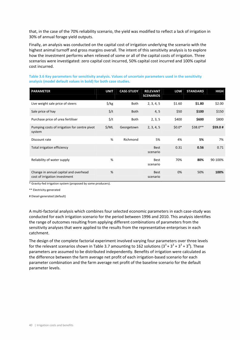
40 | Irrigation costs and benefits
that, in the case of the 70% reliability scenario, the yield was modified to reflect a lack of irrigation in 30% of annual forage yield outputs.
Finally, an analysis was conducted on the capital cost of irrigation underlying the scenario with the highest animal turnoff and gross margins overall. The intent of this sensitivity analysis is to explore how the investment performs when relieved of some or all of the capital costs of irrigation. Three scenarios were investigated: zero capital cost incurred, 50% capital cost incurred and 100% capital cost incurred.
Table 3.6 Key parameters for sensitivity analysis. Values of uncertain parameters used in the sensitivity analysis (model default values in bold) for both case studies.
PARAMETER UNIT CASE-STUDY RELEVANT SCENARIOS
LOW STANDARD HIGH
Live weight sale price of steers $/kg Both 2, 3, 4, 5 $1.60 $1.80 $2.00
Sale price of hay $/t Both 4, 5 $50 $100 $150
Purchase price of urea fertiliser $/t Both 2, 3, 5 $400 $600 $800
Pumping costs of irrigation for centre pivot system
$/ML Georgetown 2, 3, 4, 5 $0.0* $38.0** $59.0 #
Discount rate % Richmond 5% 4% 5% 7%
Total irrigation efficiency Best scenario
0.31 0.56 0.71
Reliability of water supply % Best scenario
70% 80% 90-100%
Change in annual capital and overhead cost of irrigation investment
% Best scenario
0% 50% 100%
* Gravity-fed irrigation system (proposed by some producers).
** Electricity-generated
# Diesel-generated (default)
A multi-factorial analysis which combines four selected economic parameters in each case-study was conducted for each irrigation scenario for the period between 1996 and 2010. This analysis identifies the range of outcomes resulting from applying different combinations of parameters from the sensitivity analyses that were applied to the results from the representative enterprises in each catchment.
The design of the complete factorial experiment involved varying four parameters over three levels for the relevant scenarios shown in Table 3.7 amounting to 162 solutions (33 + 33 + 33 + 34). These parameters are assumed to be distributed independently. Benefits of irrigation were calculated as the difference between the farm average net profit of each irrigation-based scenario for each parameter combination and the farm average net profit of the baseline scenario for the default parameter levels.
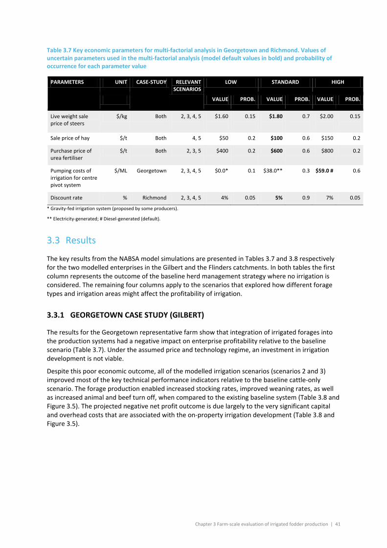
Chapter 3 Farm-scale evaluation of irrigated fodder production | 41
Table 3.7 Key economic parameters for multi-factorial analysis in Georgetown and Richmond. Values of uncertain parameters used in the multi-factorial analysis (model default values in bold) and probability of occurrence for each parameter value
PARAMETERS UNIT CASE-STUDY RELEVANT SCENARIOS
LOW STANDARD HIGH
VALUE PROB. VALUE PROB. VALUE PROB.
Live weight sale price of steers
$/kg Both 2, 3, 4, 5
$1.60
0.15
$1.80
0.7
$2.00
0.15
Sale price of hay $/t Both 4, 5 $50 0.2 $100 0.6 $150 0.2
Purchase price of urea fertiliser
$/t Both 2, 3, 5 $400 0.2 $600 0.6 $800 0.2
Pumping costs of irrigation for centre pivot system
$/ML Georgetown 2, 3, 4, 5 $0.0* 0.1 $38.0** 0.3 $59.0 # 0.6
Discount rate % Richmond 2, 3, 4, 5 4% 0.05 5% 0.9 7% 0.05
* Gravity-fed irrigation system (proposed by some producers).
** Electricity-generated; # Diesel-generated (default).
3.3 Results
The key results from the NABSA model simulations are presented in Tables 3.7 and 3.8 respectively for the two modelled enterprises in the Gilbert and the Flinders catchments. In both tables the first column represents the outcome of the baseline herd management strategy where no irrigation is considered. The remaining four columns apply to the scenarios that explored how different forage types and irrigation areas might affect the profitability of irrigation.
3.3.1 GEORGETOWN CASE STUDY (GILBERT)
The results for the Georgetown representative farm show that integration of irrigated forages into the production systems had a negative impact on enterprise profitability relative to the baseline scenario (Table 3.7). Under the assumed price and technology regime, an investment in irrigation development is not viable.
Despite this poor economic outcome, all of the modelled irrigation scenarios (scenarios 2 and 3) improved most of the key technical performance indicators relative to the baseline cattle-only scenario. The forage production enabled increased stocking rates, improved weaning rates, as well as increased animal and beef turn off, when compared to the existing baseline system (Table 3.8 and Figure 3.5). The projected negative net profit outcome is due largely to the very significant capital and overhead costs that are associated with the on-property irrigation development (Table 3.8 and Figure 3.5).
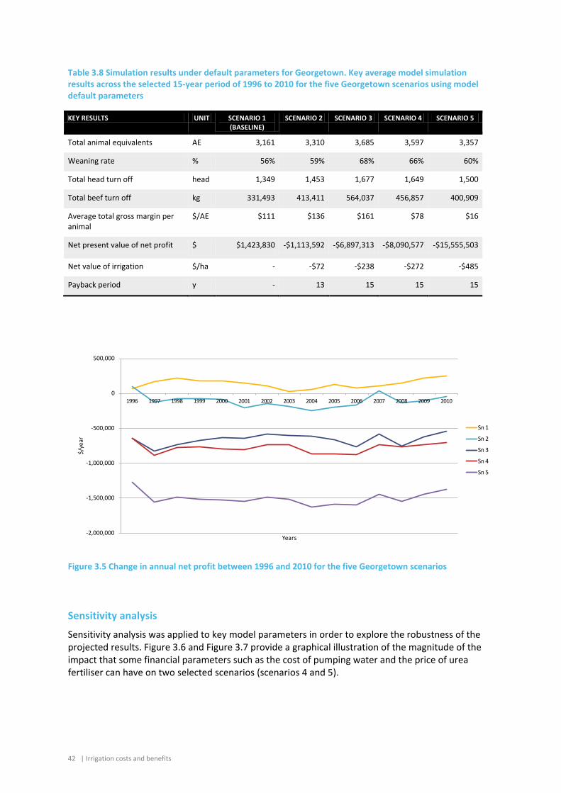
42 | Irrigation costs and benefits
Table 3.8 Simulation results under default parameters for Georgetown. Key average model simulation results across the selected 15-year period of 1996 to 2010 for the five Georgetown scenarios using model default parameters
KEY RESULTS UNIT SCENARIO 1 (BASELINE)
SCENARIO 2 SCENARIO 3 SCENARIO 4 SCENARIO 5
Total animal equivalents AE 3,161 3,310 3,685 3,597 3,357
Weaning rate % 56% 59% 68% 66% 60%
Total head turn off head 1,349 1,453 1,677 1,649 1,500
Total beef turn off kg 331,493 413,411 564,037 456,857 400,909
Average total gross margin per animal
$/AE $111 $136 $161 $78 $16
Net present value of net profit $ $1,423,830 -$1,113,592 -$6,897,313 -$8,090,577 -$15,555,503
Net value of irrigation $/ha - -$72 -$238 -$272 -$485
Payback period y - 13 15 15 15
Figure 3.5 Change in annual net profit between 1996 and 2010 for the five Georgetown scenarios
Sensitivity analysis
Sensitivity analysis was applied to key model parameters in order to explore the robustness of the projected results. Figure 3.6 and Figure 3.7 provide a graphical illustration of the magnitude of the impact that some financial parameters such as the cost of pumping water and the price of urea fertiliser can have on two selected scenarios (scenarios 4 and 5).
-2,000,000
-1,500,000
-1,000,000
-500,000
0
500,000
1996 1997 1998 1999 2000 2001 2002 2003 2004 2005 2006 2007 2008 2009 2010
$/ye
ar
Years
Sn 1
Sn 2
Sn 3
Sn 4
Sn 5
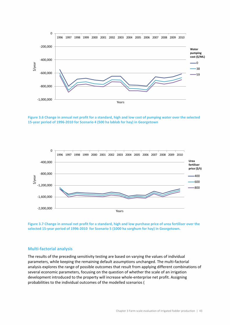
Chapter 3 Farm-scale evaluation of irrigated fodder production | 43
Figure 3.6 Change in annual net profit for a standard, high and low cost of pumping water over the selected 15-year period of 1996-2010 for Scenario 4 (500 ha lablab for hay) in Georgetown
Figure 3.7 Change in annual net profit for a standard, high and low purchase price of urea fertiliser over the selected 15-year period of 1996-2010 for Scenario 5 (1000 ha sorghum for hay) in Georgetown.
Multi-factorial analysis
The results of the preceding sensitivity testing are based on varying the values of individual parameters, while keeping the remaining default assumptions unchanged. The multi-factorial analysis explores the range of possible outcomes that result from applying different combinations of several economic parameters, focusing on the question of whether the scale of an irrigation development introduced to the property will increase whole-enterprise net profit. Assigning probabilities to the individual outcomes of the modelled scenarios (
-1,000,000
-800,000
-600,000
-400,000
-200,000
01996 1997 1998 1999 2000 2001 2002 2003 2004 2005 2006 2007 2008 2009 2010
$/ye
ar
Years
0
38
59
-2,000,000
-1,600,000
-1,200,000
-800,000
-400,000
01996 1997 1998 1999 2000 2001 2002 2003 2004 2005 2006 2007 2008 2009 2010
$/ye
ar
Years
400
600
800
Water pumping cost ($/ML)
Urea fertiliser price ($/t)
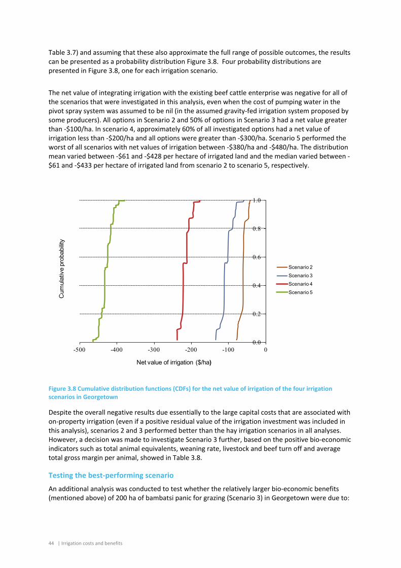
44 | Irrigation costs and benefits
Table 3.7) and assuming that these also approximate the full range of possible outcomes, the results can be presented as a probability distribution Figure 3.8. Four probability distributions are presented in Figure 3.8, one for each irrigation scenario.
The net value of integrating irrigation with the existing beef cattle enterprise was negative for all of the scenarios that were investigated in this analysis, even when the cost of pumping water in the pivot spray system was assumed to be nil (in the assumed gravity-fed irrigation system proposed by some producers). All options in Scenario 2 and 50% of options in Scenario 3 had a net value greater than -$100/ha. In scenario 4, approximately 60% of all investigated options had a net value of irrigation less than -$200/ha and all options were greater than -$300/ha. Scenario 5 performed the worst of all scenarios with net values of irrigation between -$380/ha and -$480/ha. The distribution mean varied between -$61 and -$428 per hectare of irrigated land and the median varied between -$61 and -$433 per hectare of irrigated land from scenario 2 to scenario 5, respectively.
Figure 3.8 Cumulative distribution functions (CDFs) for the net value of irrigation of the four irrigation scenarios in Georgetown
Despite the overall negative results due essentially to the large capital costs that are associated with on-property irrigation (even if a positive residual value of the irrigation investment was included in this analysis), scenarios 2 and 3 performed better than the hay irrigation scenarios in all analyses. However, a decision was made to investigate Scenario 3 further, based on the positive bio-economic indicators such as total animal equivalents, weaning rate, livestock and beef turn off and average total gross margin per animal, showed in Table 3.8.
Testing the best-performing scenario
An additional analysis was conducted to test whether the relatively larger bio-economic benefits (mentioned above) of 200 ha of bambatsi panic for grazing (Scenario 3) in Georgetown were due to:
0.0
0.2
0.4
0.6
0.8
1.0
-500 -400 -300 -200 -100 0
Cum
ulat
ive
prob
abilit
y
Net value of irrigation ($/ha)
Scenario 2
Scenario 3
Scenario 4
Scenario 5
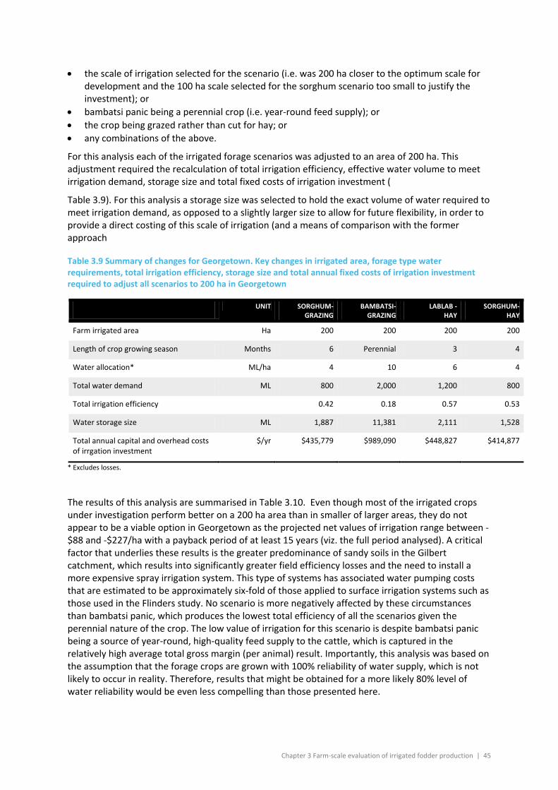
Chapter 3 Farm-scale evaluation of irrigated fodder production | 45
• the scale of irrigation selected for the scenario (i.e. was 200 ha closer to the optimum scale for development and the 100 ha scale selected for the sorghum scenario too small to justify the investment); or
• bambatsi panic being a perennial crop (i.e. year-round feed supply); or • the crop being grazed rather than cut for hay; or • any combinations of the above.
For this analysis each of the irrigated forage scenarios was adjusted to an area of 200 ha. This adjustment required the recalculation of total irrigation efficiency, effective water volume to meet irrigation demand, storage size and total fixed costs of irrigation investment (
Table 3.9). For this analysis a storage size was selected to hold the exact volume of water required to meet irrigation demand, as opposed to a slightly larger size to allow for future flexibility, in order to provide a direct costing of this scale of irrigation (and a means of comparison with the former approach
Table 3.9 Summary of changes for Georgetown. Key changes in irrigated area, forage type water requirements, total irrigation efficiency, storage size and total annual fixed costs of irrigation investment required to adjust all scenarios to 200 ha in Georgetown
UNIT SORGHUM- GRAZING
BAMBATSI- GRAZING
LABLAB - HAY
SORGHUM- HAY
Farm irrigated area Ha 200 200 200 200
Length of crop growing season Months 6 Perennial 3 4
Water allocation* ML/ha 4 10 6 4
Total water demand ML 800 2,000 1,200 800
Total irrigation efficiency 0.42 0.18 0.57 0.53
Water storage size ML 1,887 11,381 2,111 1,528
Total annual capital and overhead costs of irrgation investment
$/yr $435,779 $989,090 $448,827 $414,877
* Excludes losses.
The results of this analysis are summarised in Table 3.10. Even though most of the irrigated crops under investigation perform better on a 200 ha area than in smaller of larger areas, they do not appear to be a viable option in Georgetown as the projected net values of irrigation range between -$88 and -$227/ha with a payback period of at least 15 years (viz. the full period analysed). A critical factor that underlies these results is the greater predominance of sandy soils in the Gilbert catchment, which results into significantly greater field efficiency losses and the need to install a more expensive spray irrigation system. This type of systems has associated water pumping costs that are estimated to be approximately six-fold of those applied to surface irrigation systems such as those used in the Flinders study. No scenario is more negatively affected by these circumstances than bambatsi panic, which produces the lowest total efficiency of all the scenarios given the perennial nature of the crop. The low value of irrigation for this scenario is despite bambatsi panic being a source of year-round, high-quality feed supply to the cattle, which is captured in the relatively high average total gross margin (per animal) result. Importantly, this analysis was based on the assumption that the forage crops are grown with 100% reliability of water supply, which is not likely to occur in reality. Therefore, results that might be obtained for a more likely 80% level of water reliability would be even less compelling than those presented here.
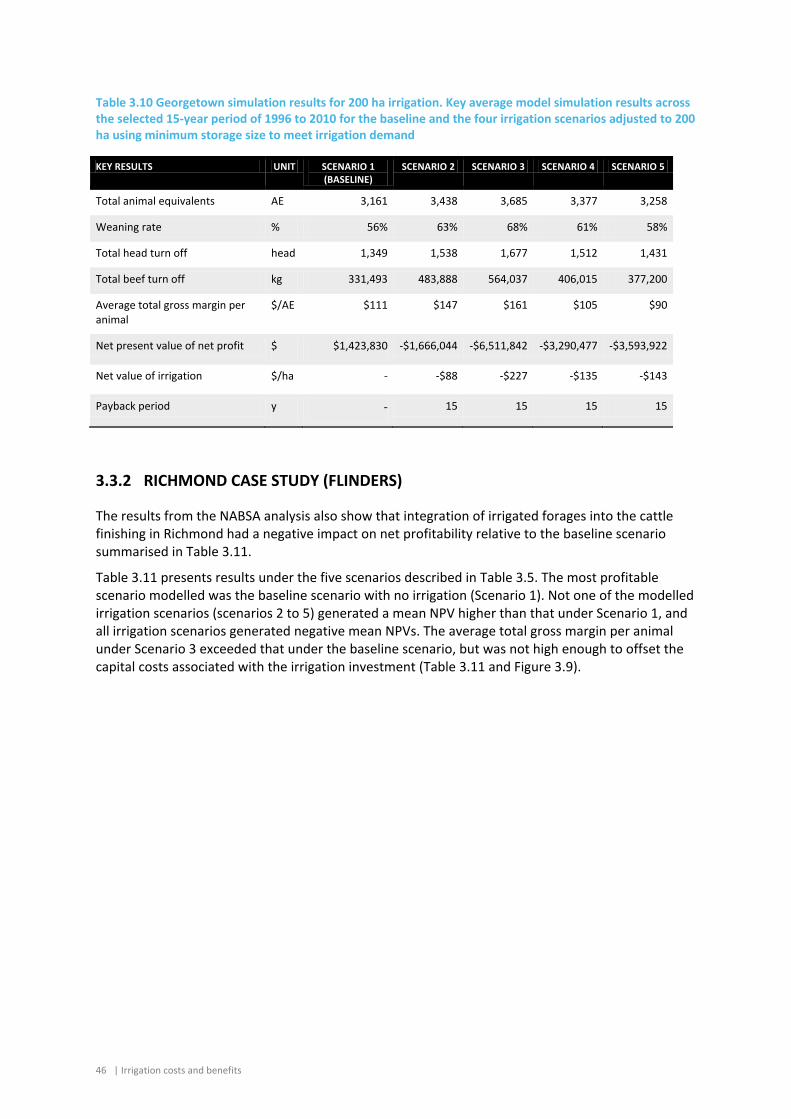
46 | Irrigation costs and benefits
Table 3.10 Georgetown simulation results for 200 ha irrigation. Key average model simulation results across the selected 15-year period of 1996 to 2010 for the baseline and the four irrigation scenarios adjusted to 200 ha using minimum storage size to meet irrigation demand
KEY RESULTS UNIT SCENARIO 1 (BASELINE)
SCENARIO 2 SCENARIO 3 SCENARIO 4 SCENARIO 5
Total animal equivalents AE 3,161 3,438 3,685 3,377 3,258
Weaning rate % 56% 63% 68% 61% 58%
Total head turn off head 1,349 1,538 1,677 1,512 1,431
Total beef turn off kg 331,493 483,888 564,037 406,015 377,200
Average total gross margin per animal
$/AE $111 $147 $161 $105 $90
Net present value of net profit $ $1,423,830 -$1,666,044 -$6,511,842 -$3,290,477 -$3,593,922
Net value of irrigation $/ha - -$88 -$227 -$135 -$143
Payback period y - 15 15 15 15
3.3.2 RICHMOND CASE STUDY (FLINDERS)
The results from the NABSA analysis also show that integration of irrigated forages into the cattle finishing in Richmond had a negative impact on net profitability relative to the baseline scenario
summarised in Table 3.11.
Table 3.11 presents results under the five scenarios described in Table 3.5. The most profitable scenario modelled was the baseline scenario with no irrigation (Scenario 1). Not one of the modelled irrigation scenarios (scenarios 2 to 5) generated a mean NPV higher than that under Scenario 1, and all irrigation scenarios generated negative mean NPVs. The average total gross margin per animal under Scenario 3 exceeded that under the baseline scenario, but was not high enough to offset the capital costs associated with the irrigation investment (Table 3.11 and Figure 3.9).
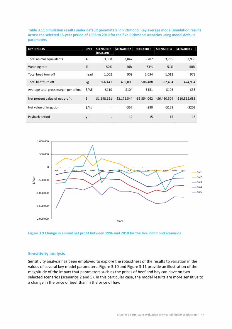
Chapter 3 Farm-scale evaluation of irrigated fodder production | 47
Table 3.11 Simulation results under default parameters in Richmond. Key average model simulation results across the selected 15-year period of 1996 to 2010 for the five Richmond scenarios using model default parameters
KEY RESULTS UNIT SCENARIO 1 (BASELINE)
SCENARIO 2 SCENARIO 3 SCENARIO 4 SCENARIO 5
Total animal equivalents AE 3,558 3,847 3,707 3,785 3,936
Weaning rate % 50% 46% 51% 51% 50%
Total head turn off head 1,002 909 1,034 1,012 973
Total beef turn off kg 366,441 409,803 506,488 502,404 474,934
Average total gross margin per animal $/AE $110 $104 $151 $103 $35
Net present value of net profit $ $1,248,651 -$2,175,544 -$3,554,062 -$6,480,504 -$10,855,681
Net value of irrigation $/ha - -$57 -$80 -$129 -$202
Payback period y - 12 15 15 15
Figure 3.9 Change in annual net profit between 1996 and 2010 for the five Richmond scenarios
Sensitivity analysis
Sensitivity analysis has been employed to explore the robustness of the results to variation in the values of several key model parameters. Figure 3.10 and Figure 3.11 provide an illustration of the magnitude of the impact that parameters such as the prices of beef and hay can have on two selected scenarios (scenarios 2 and 5). In this particular case, the model results are more sensitive to a change in the price of beef than in the price of hay.
-2,000,000
-1,500,000
-1,000,000
-500,000
0
500,000
1,000,000
1996 1997 1998 1999 2000 2001 2002 2003 2004 2005 2006 2007 2008 2009 2010
$/ye
ar
Years
Sn 1
Sn 2
Sn 3
Sn 4
Sn 5
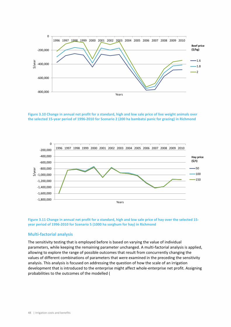
48 | Irrigation costs and benefits
Figure 3.10 Change in annual net profit for a standard, high and low sale price of live weight animals over the selected 15-year period of 1996-2010 for Scenario 2 (200 ha bambatsi panic for grazing) in Richmond
Figure 3.11 Change in annual net profit for a standard, high and low sale price of hay over the selected 15-year period of 1996-2010 for Scenario 5 (1000 ha sorghum for hay) in Richmond
Multi-factorial analysis
The sensitivity testing that is employed before is based on varying the value of individual parameters, while keeping the remaining parameter unchanged. A multi-factorial analysis is applied, allowing to explore the range of possible outcomes that result from concurrently changing the values of different combinations of parameters that were examined in the preceding the sensitivity analysis. This analysis is focused on addressing the question of how the scale of an irrigation development that is introduced to the enterprise might affect whole-enterprise net profit. Assigning probabilities to the outcomes of the modelled (
-800,000
-600,000
-400,000
-200,000
01996 1997 1998 1999 2000 2001 2002 2003 2004 2005 2006 2007 2008 2009 2010
$/ye
ar
Years
1.6
1.8
2
-1,800,000
-1,600,000
-1,400,000
-1,200,000
-1,000,000
-800,000
-600,000
-400,000
-200,000
01996 1997 1998 1999 2000 2001 2002 2003 2004 2005 2006 2007 2008 2009 2010
$/ye
ar
Years
50
100
150
Beef price ($/kg)
Hay price ($/t)
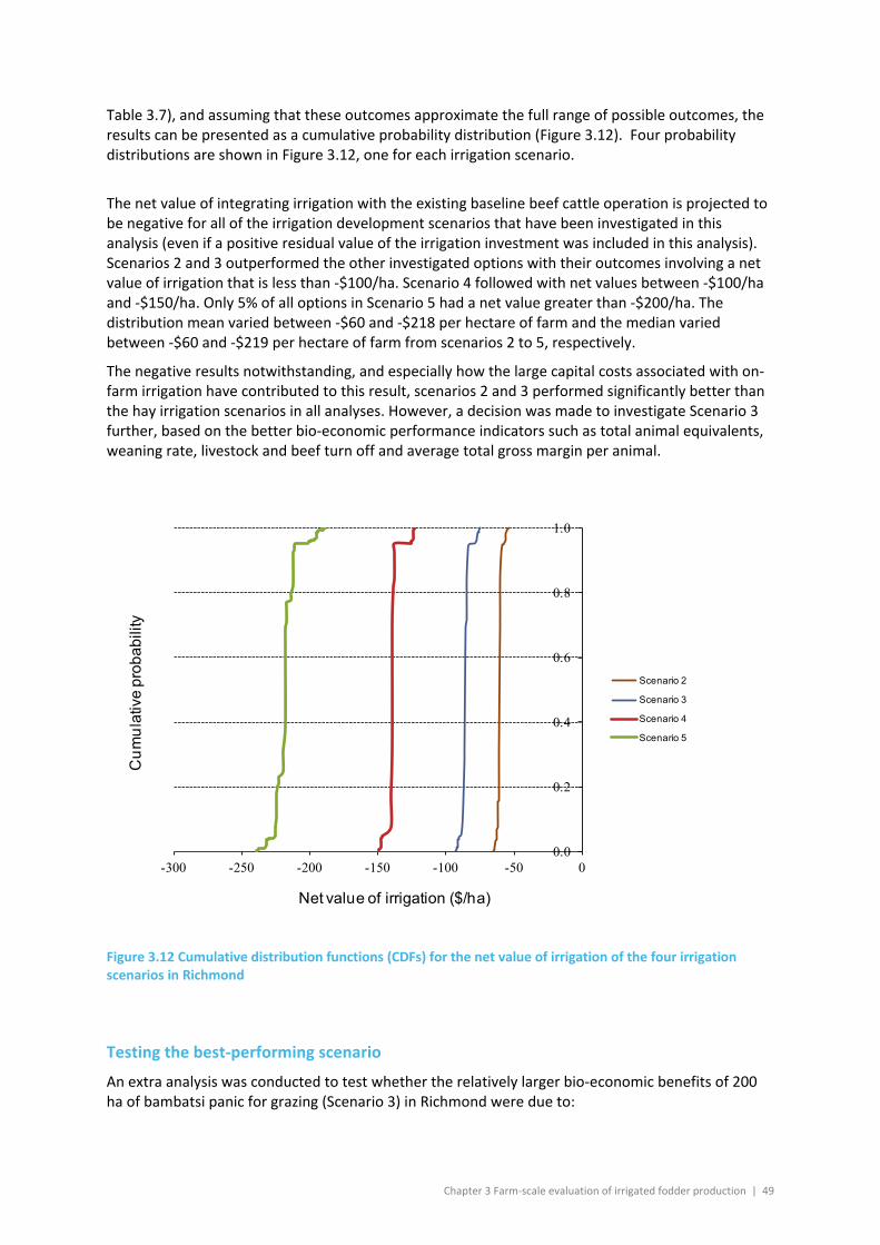
Chapter 3 Farm-scale evaluation of irrigated fodder production | 49
Table 3.7), and assuming that these outcomes approximate the full range of possible outcomes, the results can be presented as a cumulative probability distribution (Figure 3.12). Four probability distributions are shown in Figure 3.12, one for each irrigation scenario.
The net value of integrating irrigation with the existing baseline beef cattle operation is projected to be negative for all of the irrigation development scenarios that have been investigated in this analysis (even if a positive residual value of the irrigation investment was included in this analysis). Scenarios 2 and 3 outperformed the other investigated options with their outcomes involving a net value of irrigation that is less than -$100/ha. Scenario 4 followed with net values between -$100/ha and -$150/ha. Only 5% of all options in Scenario 5 had a net value greater than -$200/ha. The distribution mean varied between -$60 and -$218 per hectare of farm and the median varied between -$60 and -$219 per hectare of farm from scenarios 2 to 5, respectively.
The negative results notwithstanding, and especially how the large capital costs associated with on-farm irrigation have contributed to this result, scenarios 2 and 3 performed significantly better than the hay irrigation scenarios in all analyses. However, a decision was made to investigate Scenario 3 further, based on the better bio-economic performance indicators such as total animal equivalents, weaning rate, livestock and beef turn off and average total gross margin per animal.
Figure 3.12 Cumulative distribution functions (CDFs) for the net value of irrigation of the four irrigation scenarios in Richmond
Testing the best-performing scenario
An extra analysis was conducted to test whether the relatively larger bio-economic benefits of 200 ha of bambatsi panic for grazing (Scenario 3) in Richmond were due to:
0.0
0.2
0.4
0.6
0.8
1.0
-300 -250 -200 -150 -100 -50 0
Cum
ulat
ive
prob
abili
ty
Net value of irrigation ($/ha)
Scenario 2
Scenario 3
Scenario 4
Scenario 5
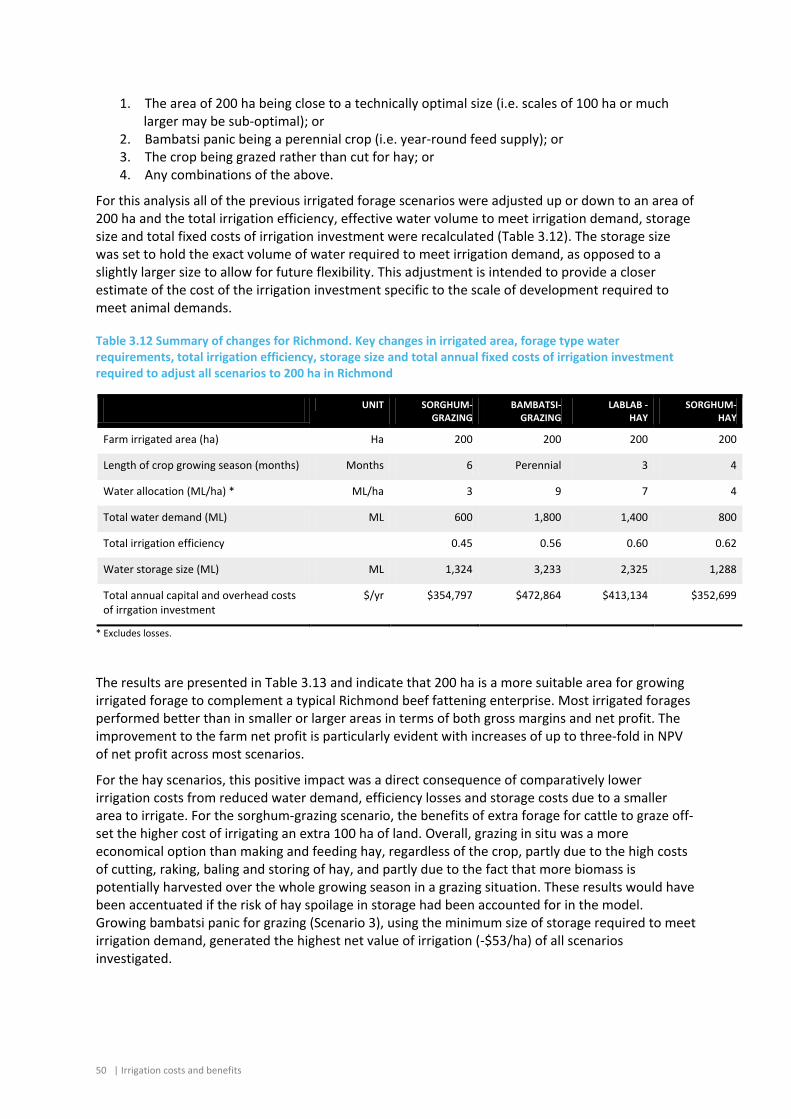
50 | Irrigation costs and benefits
1. The area of 200 ha being close to a technically optimal size (i.e. scales of 100 ha or much larger may be sub-optimal); or
2. Bambatsi panic being a perennial crop (i.e. year-round feed supply); or 3. The crop being grazed rather than cut for hay; or 4. Any combinations of the above.
For this analysis all of the previous irrigated forage scenarios were adjusted up or down to an area of 200 ha and the total irrigation efficiency, effective water volume to meet irrigation demand, storage size and total fixed costs of irrigation investment were recalculated (Table 3.12). The storage size was set to hold the exact volume of water required to meet irrigation demand, as opposed to a slightly larger size to allow for future flexibility. This adjustment is intended to provide a closer estimate of the cost of the irrigation investment specific to the scale of development required to meet animal demands.
Table 3.12 Summary of changes for Richmond. Key changes in irrigated area, forage type water requirements, total irrigation efficiency, storage size and total annual fixed costs of irrigation investment required to adjust all scenarios to 200 ha in Richmond
UNIT SORGHUM- GRAZING
BAMBATSI- GRAZING
LABLAB - HAY
SORGHUM- HAY
Farm irrigated area (ha) Ha 200 200 200 200
Length of crop growing season (months) Months 6 Perennial 3 4
Water allocation (ML/ha) * ML/ha 3 9 7 4
Total water demand (ML) ML 600 1,800 1,400 800
Total irrigation efficiency 0.45 0.56 0.60 0.62
Water storage size (ML) ML 1,324 3,233 2,325 1,288
Total annual capital and overhead costs of irrgation investment
$/yr $354,797 $472,864 $413,134 $352,699
* Excludes losses.
The results are presented in Table 3.13 and indicate that 200 ha is a more suitable area for growing irrigated forage to complement a typical Richmond beef fattening enterprise. Most irrigated forages performed better than in smaller or larger areas in terms of both gross margins and net profit. The improvement to the farm net profit is particularly evident with increases of up to three-fold in NPV of net profit across most scenarios.
For the hay scenarios, this positive impact was a direct consequence of comparatively lower irrigation costs from reduced water demand, efficiency losses and storage costs due to a smaller area to irrigate. For the sorghum-grazing scenario, the benefits of extra forage for cattle to graze off-set the higher cost of irrigating an extra 100 ha of land. Overall, grazing in situ was a more economical option than making and feeding hay, regardless of the crop, partly due to the high costs of cutting, raking, baling and storing of hay, and partly due to the fact that more biomass is potentially harvested over the whole growing season in a grazing situation. These results would have been accentuated if the risk of hay spoilage in storage had been accounted for in the model. Growing bambatsi panic for grazing (Scenario 3), using the minimum size of storage required to meet irrigation demand, generated the highest net value of irrigation (-$53/ha) of all scenarios investigated.
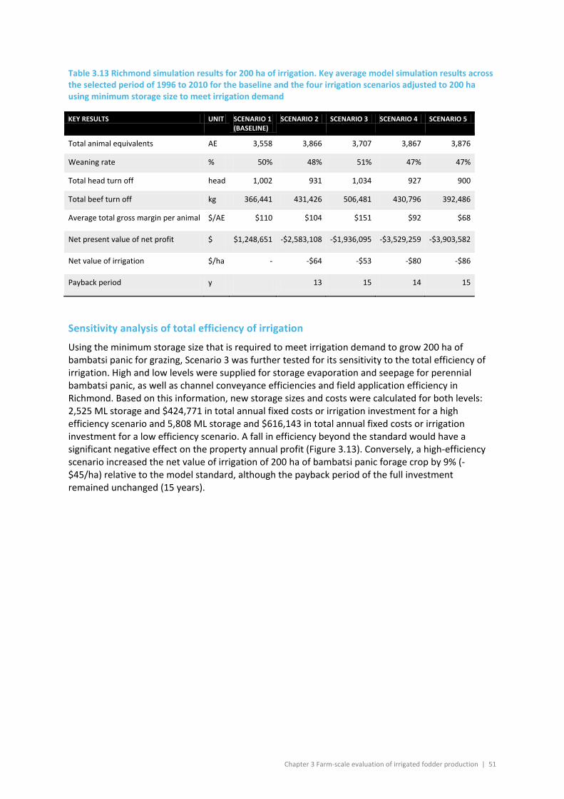
Chapter 3 Farm-scale evaluation of irrigated fodder production | 51
Table 3.13 Richmond simulation results for 200 ha of irrigation. Key average model simulation results across the selected period of 1996 to 2010 for the baseline and the four irrigation scenarios adjusted to 200 ha using minimum storage size to meet irrigation demand
KEY RESULTS UNIT SCENARIO 1 (BASELINE)
SCENARIO 2 SCENARIO 3 SCENARIO 4 SCENARIO 5
Total animal equivalents AE 3,558 3,866 3,707 3,867 3,876
Weaning rate % 50% 48% 51% 47% 47%
Total head turn off head 1,002 931 1,034 927 900
Total beef turn off kg 366,441 431,426 506,481 430,796 392,486
Average total gross margin per animal $/AE $110 $104 $151 $92 $68
Net present value of net profit $ $1,248,651 -$2,583,108 -$1,936,095 -$3,529,259 -$3,903,582
Net value of irrigation $/ha - -$64 -$53 -$80 -$86
Payback period y 13 15 14 15
Sensitivity analysis of total efficiency of irrigation
Using the minimum storage size that is required to meet irrigation demand to grow 200 ha of bambatsi panic for grazing, Scenario 3 was further tested for its sensitivity to the total efficiency of irrigation. High and low levels were supplied for storage evaporation and seepage for perennial bambatsi panic, as well as channel conveyance efficiencies and field application efficiency in Richmond. Based on this information, new storage sizes and costs were calculated for both levels: 2,525 ML storage and $424,771 in total annual fixed costs or irrigation investment for a high efficiency scenario and 5,808 ML storage and $616,143 in total annual fixed costs or irrigation investment for a low efficiency scenario. A fall in efficiency beyond the standard would have a significant negative effect on the property annual profit (Figure 3.13). Conversely, a high-efficiency scenario increased the net value of irrigation of 200 ha of bambatsi panic forage crop by 9% (-$45/ha) relative to the model standard, although the payback period of the full investment remained unchanged (15 years).
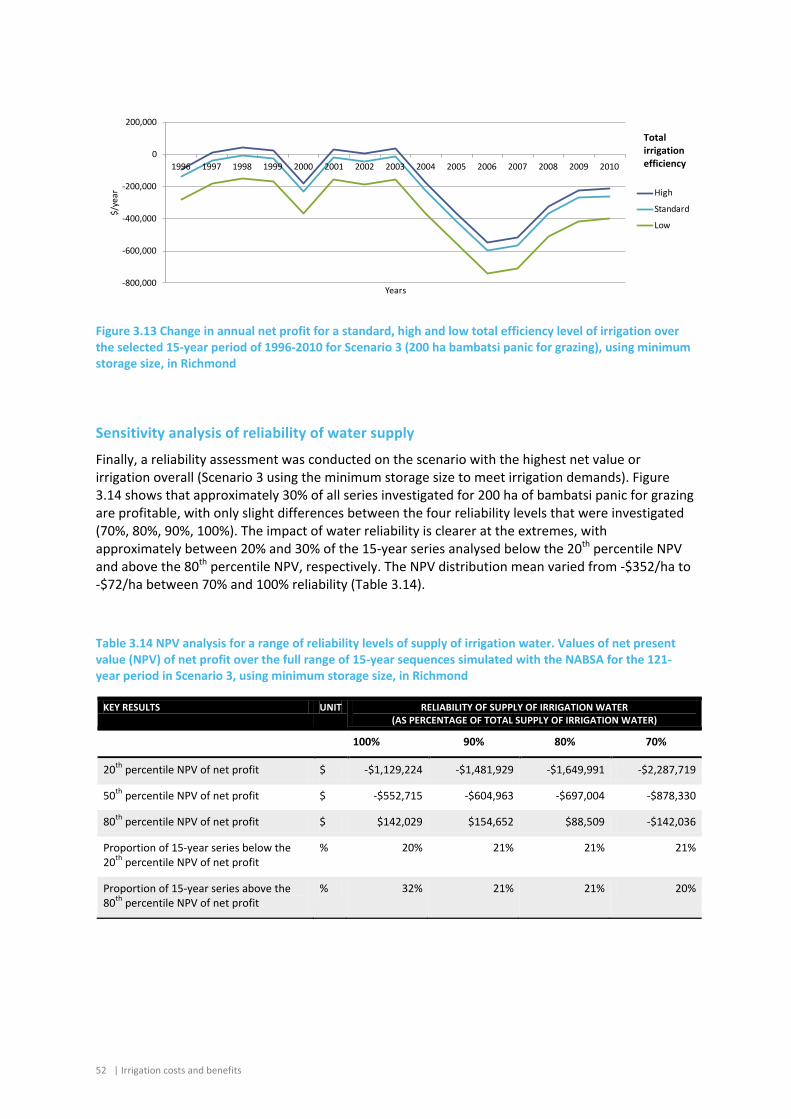
52 | Irrigation costs and benefits
Figure 3.13 Change in annual net profit for a standard, high and low total efficiency level of irrigation over the selected 15-year period of 1996-2010 for Scenario 3 (200 ha bambatsi panic for grazing), using minimum storage size, in Richmond
Sensitivity analysis of reliability of water supply
Finally, a reliability assessment was conducted on the scenario with the highest net value or irrigation overall (Scenario 3 using the minimum storage size to meet irrigation demands). Figure 3.14 shows that approximately 30% of all series investigated for 200 ha of bambatsi panic for grazing are profitable, with only slight differences between the four reliability levels that were investigated (70%, 80%, 90%, 100%). The impact of water reliability is clearer at the extremes, with approximately between 20% and 30% of the 15-year series analysed below the 20th percentile NPV and above the 80th percentile NPV, respectively. The NPV distribution mean varied from -$352/ha to -$72/ha between 70% and 100% reliability (Table 3.14).
Table 3.14 NPV analysis for a range of reliability levels of supply of irrigation water. Values of net present value (NPV) of net profit over the full range of 15-year sequences simulated with the NABSA for the 121-year period in Scenario 3, using minimum storage size, in Richmond
KEY RESULTS UNIT RELIABILITY OF SUPPLY OF IRRIGATION WATER (AS PERCENTAGE OF TOTAL SUPPLY OF IRRIGATION WATER)
100% 90% 80% 70%
20th percentile NPV of net profit $ -$1,129,224 -$1,481,929 -$1,649,991 -$2,287,719
50th percentile NPV of net profit $ -$552,715 -$604,963 -$697,004 -$878,330
80th percentile NPV of net profit $ $142,029 $154,652 $88,509 -$142,036
Proportion of 15-year series below the 20th percentile NPV of net profit
% 20% 21% 21% 21%
Proportion of 15-year series above the 80th percentile NPV of net profit
% 32% 21% 21% 20%
-800,000
-600,000
-400,000
-200,000
0
200,000
1996 1997 1998 1999 2000 2001 2002 2003 2004 2005 2006 2007 2008 2009 2010
$/ye
ar
Years
High
Standard
Low
Total irrigation efficiency
Chapter 3 Farm-scale evaluation of irrigated fodder production | 53
Figure 3.14 Cumulative distribution functions (CDFs) for a standard, high and low levels of reliability of water supply for the 107 streams of 15 years over the period of 1890 to 2010 for Scenario 3 (200 ha bambatsi panic for grazing), using minimum storage size, in Richmond.
Sensitivity analysis of capital costs of irrigation
From the results shown in Table 3.15 it is clear that even a 50% reduction in capital costs fails to generate an NPV of net profit higher than the baseline scenario. In the complete absence of capital cost outlays, the 200 ha of irrigated forage crop results in higher net profits than the baseline scenario.
Table 3.15 Simulated results for three levels of irrigation costs on the scenario with the overall highest net value of irrigation. Key average economic results across the selected 15-year period of 1996 to 2010 for the Richmond scenario with 200 ha of bambatsi panic for grazing using minimum storage size to meet irrigation demand. Results for the baseline scenario are included for reference.
KEY RESULTS UNIT SCENARIO 1 (BASELINE)
CAPITAL COSTS FOR IRRIGATION (AS PERCENTAGE OF TOTAL COST OF IRRIGATION)
100% 50% 0%
Net present value of net profit $ $1,248,651 -$1,936,095 $517,988 $2,972,072
Net value of irrigation $/ha - -$53 -$12 $29
Payback period y - 15 6 2
0
10
20
30
40
50
60
70
80
90
100
-100 -80 -60 -40 -20 0 20 40
Cum
ulat
ive
prob
abili
ty
NPV ($/ha)
70
80
90
100
Reliability of water supply (%)
54 | Irrigation costs and benefits
3.4 Discussion
The benefits of irrigated forage resulted from the intensification of beef cattle production by means of overcoming seasonal feed shortages. Notably, the main economic value of irrigation accrues from:
1. Higher turnoff weight fetching a higher price per head in the market achieved through a combination of longer fattening period and increased daily live weight gain as a result of a more reliable and abundant source of feed supply;
2. Reduced need for costly supplementary feed, such as grain and purchased hay, during the dry season due to provision of on-farm valuable feed;
3. Sale of hay as a complementary source of revenue;
The reported increases in revenue from livestock and/or hay sale were partly off-set by higher forage input costs, livestock husbandry and replacement costs, as well as extra labour and freight costs.
The capital costs of irrigation are a significant burden on the business net profit and far outweighed the benefits of growing approximately 200 ha of a forage crop on the property to complement especially the fattening enterprise in the Flinders catchment.
Previous economic assessments conducted in the Flinders catchment (e.g. Mason and Larard, 2011) present analyses of irrigation investments for irrigating forage crops which have higher returns than the findings presented in this report. The differences can be explained by different assumptions and analysis design. A key difference between the studies is the size of on-farm storage modelled. Much larger (and therefore more expensive) storages are modelled in this study, reflecting the assumptions made about water losses in the system.
The studies are in agreement that irrigated forage can potentially deliver benefits at the property scale in the form of increased revenues from cattle sales, but that water reliability, irrigation efficiency, and production variability are significant issues affecting the profitability of an investment in irrigation.
3.5 Conclusion
The utilisation of irrigated forage increased the productivity of the cattle herds modelled in this analysis, through the provision of more and better quality feed. Under the parameters of this analysis, however, the costs of providing irrigated forage outweighed the gains. This is due to the large capital costs associated with irrigation development at the property scale.
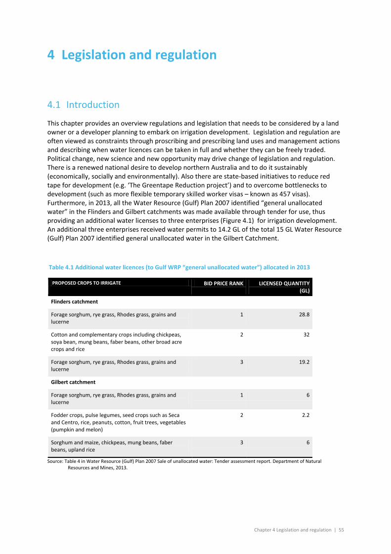
Chapter 4 Legislation and regulation | 55
4 Legislation and regulation
4.1 Introduction
This chapter provides an overview regulations and legislation that needs to be considered by a land owner or a developer planning to embark on irrigation development. Legislation and regulation are often viewed as constraints through proscribing and prescribing land uses and management actions and describing when water licences can be taken in full and whether they can be freely traded. Political change, new science and new opportunity may drive change of legislation and regulation. There is a renewed national desire to develop northern Australia and to do it sustainably (economically, socially and environmentally). Also there are state-based initiatives to reduce red tape for development (e.g. ‘The Greentape Reduction project’) and to overcome bottlenecks to development (such as more flexible temporary skilled worker visas – known as 457 visas). Furthermore, in 2013, all the Water Resource (Gulf) Plan 2007 identified “general unallocated water” in the Flinders and Gilbert catchments was made available through tender for use, thus providing an additional water licenses to three enterprises (Figure 4.1) for irrigation development. An additional three enterprises received water permits to 14.2 GL of the total 15 GL Water Resource (Gulf) Plan 2007 identified general unallocated water in the Gilbert Catchment.
Table 4.1 Additional water licences (to Gulf WRP “general unallocated water”) allocated in 2013
PROPOSED CROPS TO IRRIGATE BID PRICE RANK LICENSED QUANTITY (GL)
Flinders catchment
Forage sorghum, rye grass, Rhodes grass, grains and lucerne
1 28.8
Cotton and complementary crops including chickpeas, soya bean, mung beans, faber beans, other broad acre crops and rice
2 32
Forage sorghum, rye grass, Rhodes grass, grains and lucerne
3 19.2
Gilbert catchment
Forage sorghum, rye grass, Rhodes grass, grains and lucerne
1 6
Fodder crops, pulse legumes, seed crops such as Seca and Centro, rice, peanuts, cotton, fruit trees, vegetables (pumpkin and melon)
2 2.2
Sorghum and maize, chickpeas, mung beans, faber beans, upland rice
3 6
Source: Table 4 in Water Resource (Gulf) Plan 2007 Sale of unallocated water: Tender assessment report. Department of Natural Resources and Mines, 2013.
56 | Irrigation costs and benefits
4.2 Legislation and regulation
4.2.1 WATER
Queensland’s Water Act 2000 is the authorising law – other legislation described in this section is subordinate legislation and includes:
• Water Act 2000 (Qld) – herewith referred to as Water Act (Qld) • Water Resource (Great Artesian Basin) Plan 2006 – herewith referred to as Great Artesian Basin
WRP or GAB WRP
– Great Artesian Basin Resource Operations Plan 2006 – herewith referred to as Great Artesian Basin ROP or GAB ROP
• Water Resource (Gulf) Plan 2007 – herewith referred to as Gulf WRP
– Gulf Resource Operations Plan 2010 – herewith referred to as Gulf ROP
• Sustainable Planning Act 2009 (Qld) – herewith referred to as Sustainable Planning Act (Qld)
The economic and development priorities in the catchments of the Flinders and Gilbert rivers are clearly identified in the water planning documents that support the Water Act (Qld). For example, the Gulf WRP (Clause 13) lists 16 outcomes for water development sought under the plan. The outcomes pertain to development that is environmentally sustainable, culturally sensitive, and socially and economically sensible.
Water Act (Qld)
The Act provides for the sustainable allocation and management of water to meet Queensland’s future water needs (DNRME, 2004). It governs water licences, water allocations (the volumes of water made available by the State for allocation in any year may be different to licensed permit volumes to take account of water supply conditions) and the preparation and implementation of water resource plans (WRPs) and resource operation plans (ROPs) as well as regulating the water industry and water service providers. The Act permits water extraction (diversion from a river or the pumping of groundwater) for stock and domestic use without a water permit but for all other purposes a water permit is required. There are three water permit categories: (1) water licences are attached to land, valid for 5 to 10 years, non-tradeable in most cases, and are conditional (i.e. maximum annual volume, maximum rate of extraction, minimum stream flow for extraction and purpose), (2) water allocations are not attached to land, can either be supplemented allocations (i.e. supplied from a water supply scheme) or unsupplemented allocations (i.e. supplied from natural river flow or groundwater), do not expire and may be traded in accordance with relevant WRPs and (3) water permits are entitlements that are granted usually for less than a year (e.g. for construction purposes).The type of water licence determines the flexibility of water use and the conditions attached to the licence, if any, will determine the security of the water supply to the licence owner.
To develop a water licence, the legislation requires an individual to apply for a water licence under the Water Act (Qld) as well as for development permission under the Sustainable Planning Act (Qld).
Water Resource (Great Artesian Basin) Plan 2006 and Great Artesian Basin Resource Operations Plan 2006 (amended 2012)
Within the GAB a permit is required to extract water from a bore except for domestic purposes. Water can be relocated by transferring, amending or amalgamating part or all of a water licence. Relocation of a water licence transfers ownership of the entitlement from the land to which it was attached to another parcel(s) of land. Water allocations cannot be traded independently of land titles. Section 47 of the GAB ROP lists a set of rules for the relocation of water licences.
Chapter 4 Legislation and regulation | 57
The GAB WRP has been developed to protect springs and other groundwater-dependent ecosystems, secure water availability for existing users and provide mechanisms to release limited volumes of groundwater for new users. It defines the availability of water in the plan area; provides a framework for sustainably managing water and the taking of water and identifies priorities and mechanisms for dealing with future water requirements (Section 2).
To streamline the process for release of unallocated water, the GAB ROP was amended in 2012. Unallocated water available for release is listed by WRP-defined management areas in Schedule 5 of the GAB WRP – there are 2000 ML of GAB unallocated water in the WRP-defined Flinders management area.
Water Resource (Gulf) Plan 2007
The Gulf WRP provides the water resource planning framework for the Flinders River and Gilbert River Catchment Area as well as six other catchment areas (Settlement Creek, Nicholson River, Leichhardt River, Morning Inlet, Norman River, and Staaten River) that flow into the Gulf of Carpentaria, and groundwater that is not connected to sub-artesian or artesian water managed under the GAB WRP. The Gulf WRP lists social, economic, cultural and ecological outcomes to be achieved under the plan (Clauses 13 to 16) which include irrigation development in the Flinders Catchment Area (Clause 13 s i). These outcomes are to be achieved by a suite of environmental flow (low flow and medium to high flow) objectives (see, Gulf WRP, Section 17 to 18 and Schedule 5) and water allocation security objectives (see, Gulf WRP, Section 19 to 20 and Schedule 6) with supporting strategies to achieve the outcomes (see, Gulf WRP, Chapter 5) such as measuring devices, environmental management rules and water sharing rules (see, Gulf WRP, Section 22 to 24).
Under the Gulf WRP, Clause 13 (i) there is specific mention to make water available to support growth in irrigated agriculture in the Flinders River and Gilbert River catchment areas. Section 29(1) of the WRP also governs how unallocated (surface) water held as indigenous, strategic or general reserve may be granted from the reserve (i.e. through the granting of a water licence under a resource operations plan) and additional requirements for unallocated groundwater in the Einasleigh groundwater management area in the Gilbert River catchment area (Section 31). The volumes of unallocated water are listed in the Plan Schedules. For the Flinders River Catchment Area, 80 GL of water, and for the Gilbert River Catchment Area, 15 GL of water, was identified as ‘General Unallocated’. In July 2012, a process for releasing this unallocated water by tender commenced. Water licences were granted to six successful bidders in May 2013, of which three were in the Flinders River Catchment Area and three were in the Gilbert River Catchment Area (see Table 4.1).
The WRP will be reviewed in 2017, or earlier, if a decision is taken by the Minister for Natural Resources and Mines.
Gulf Resource Operations Plan 2010
The Gulf ROP is consistent with the policy objectives of the Water Act (Qld) and implements the Gulf WRP. A goal of the plan is to provide for the sustainable management of water by:
a. allowing for the allocation of water and contributing to the fair, orderly and efficient allocation of water to meet community needs
b. protecting the biological diversity and health of natural ecosystems and contributing to the protection and, where possible, reversal of degradation of water, watercourses, lakes, springs, aquifers, natural ecosystems and other resources
c. contributing to improving the confidence of water users regarding the availability and security of water entitlements (including by (i) stating a process for dealing with unallocated water)
58 | Irrigation costs and benefits
d. contributing to increasing community understanding and participation in the sustainable management of water (Clause 16).
The process for allocating general unallocated water is described in detail (see, Clauses 30 to 35). Information requirements to develop water include land suitability (specifically the availability of land without remnant vegetation), the occurrence of ecological assets such as wetlands, suitability of topography, known cultural heritage sites, information on soil attributes. In all cases applicants for water licences must develop a land and water management plan. The Gulf ROP also includes provisions for water trading for water and natural ecosystems monitoring and reporting requirements.
Gulf region general unallocated water release
In 2012, following on from the Gulf WRP and ROP processes which set the reserve volumes and developed processes for general unallocated water release, an administrative process to release unallocated general reserve water in the Flinders and Gilbert Rivers Catchment Areas commenced. There were public information forums (advertised by public notice, media release and local governments) about the water release and tender documents (DNRM, 2012) and information made available online and through Department of Natural Resources and Mines (DNRM) extension staff. As per the WRP, the entire 80 GL general reserve was available for release in the Flinders River Catchment Area and the entire 15 GL general reserve was available for release in the Gilbert River Catchment Area. General unallocated water was released via a tender process. Applications were due on 26 October 2012.
The released water was for ‘rural’ purposes (i.e. agriculture and aquaculture). The DNRM had clear published criteria for acceptance of bids and for dealing with an oversubscribed tender. Applicants were limited to a maximum tender of 32 GL in the Flinders River Catchment Area. Each bid had to meet the (unknown) reserve price and each bid was ranked by reserve price. Bids had to meet the tender criteria – for instance, each bidder had to have land tenure and identify suitable land for irrigation or aquaculture, had to identify any known Indigenous values (DNRM, 2012, Schedule 2) and had to detail the proponent’s development plan including details of the infrastructure for taking and storing water and the proposed timeframe for development.
As part of the release, the department had to make assumptions about future possible uses in the catchment area given the current low utilisation of water licences in the Gulf WRP. This low utilisation rate results from a large proportion of sleeper and dozer licences (licences that are not yet activated but could be) as well as less than full utilisation of licences that could be fully activated for irrigated agriculture. There are currently a very large 26.6 GL of such licences in the Flinders catchment. The Queensland government modelled the Flinders River and made plans assuming these licences were activated (e.g. defining flow rules to ensure meeting the water requirements of waterholes, bed sands and existing licences and including sleeper volumes). From their knowledge of the catchment hydrology and through discussions with potential bidders, DNRM was unconcerned about geographically concentrated demand and any mismatch between demand and stream flow.
The water licences that were allocated in 2013 are for a specific volume, an authorised activity attached to a specified parcel(s) of land, for an authorised purpose (rural), and with set daily extraction limits. The flow conditions attached to the licence will guarantee the medium–high flows of the flow regime needed to maintain waterholes and bed sands as well as the flood flows which connect the river to floodplains and maintain vegetation and cultural sites. Those who won the tender can engage in a process to renew as the licence expiry date approaches.
Twenty-two applications were received, of which 18 were in the Flinders River catchment. A total of six new water licences in both catchments were announced in late May 2013 totalling 94.2 GL, of which the entire 80 GL general unallocated water in the Flinders River catchment was released and 12.2 GL of the 15 GL in the Gilbert River catchment. See Table 4.1. As per the tender documents
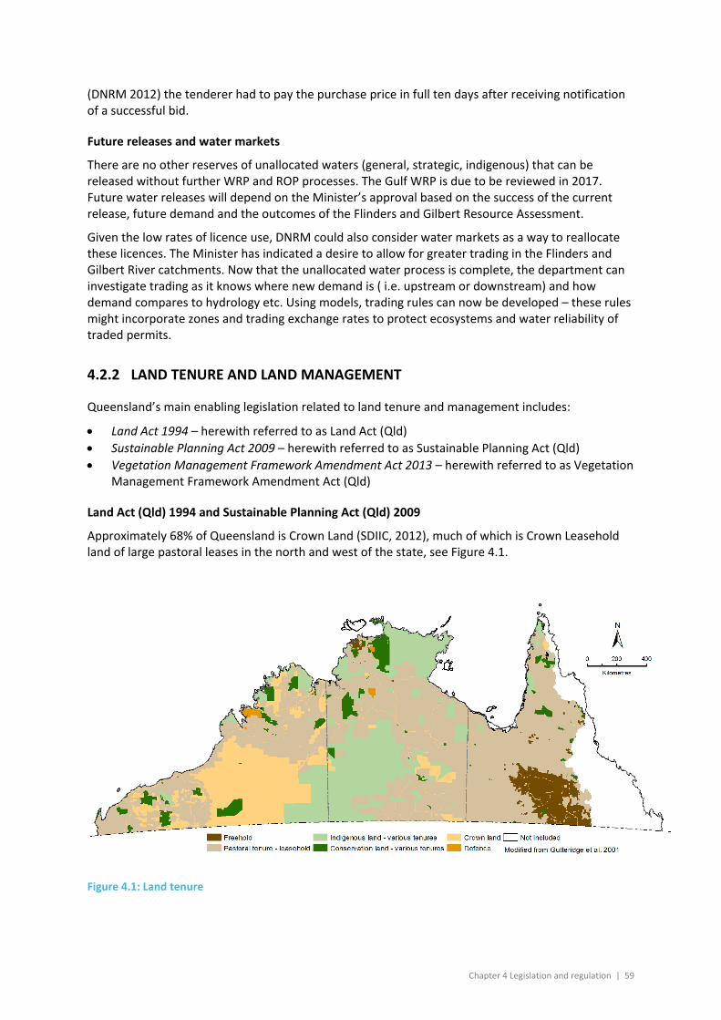
Chapter 4 Legislation and regulation | 59
(DNRM 2012) the tenderer had to pay the purchase price in full ten days after receiving notification of a successful bid.
Future releases and water markets
There are no other reserves of unallocated waters (general, strategic, indigenous) that can be released without further WRP and ROP processes. The Gulf WRP is due to be reviewed in 2017. Future water releases will depend on the Minister’s approval based on the success of the current release, future demand and the outcomes of the Flinders and Gilbert Resource Assessment.
Given the low rates of licence use, DNRM could also consider water markets as a way to reallocate these licences. The Minister has indicated a desire to allow for greater trading in the Flinders and Gilbert River catchments. Now that the unallocated water process is complete, the department can investigate trading as it knows where new demand is ( i.e. upstream or downstream) and how demand compares to hydrology etc. Using models, trading rules can now be developed – these rules might incorporate zones and trading exchange rates to protect ecosystems and water reliability of traded permits.
4.2.2 LAND TENURE AND LAND MANAGEMENT
Queensland’s main enabling legislation related to land tenure and management includes:
• Land Act 1994 – herewith referred to as Land Act (Qld) • Sustainable Planning Act 2009 – herewith referred to as Sustainable Planning Act (Qld) • Vegetation Management Framework Amendment Act 2013 – herewith referred to as Vegetation
Management Framework Amendment Act (Qld)
Land Act (Qld) 1994 and Sustainable Planning Act (Qld) 2009
Approximately 68% of Queensland is Crown Land (SDIIC, 2012), much of which is Crown Leasehold land of large pastoral leases in the north and west of the state, see Figure 4.1.
Figure 4.1: Land tenure
60 | Irrigation costs and benefits
Pastoral land is considered privately managed land and is administered as leasehold land under the Land Act (Qld). A key difference between leasehold and freehold land tenure is that lessees must comply with the purpose and conditions of the lease and the provisions of the Land Act (Qld) (SDIIC, 2012:9). Therefore, leaseholders wishing to develop irrigated agriculture on a leasehold property need to consider land tenure regulations and associated permits. Depending on the tenure of an individual’s property, the number and type of permits required will vary (Table 4.2). Note that development on land, whether the property is freehold or leasehold, must be consistent with the Sustainable Planning Act (Qld). Assessable land development (e.g. reconfiguration of a lot, building works, material change of land use, plumbing and drainage works, etc) must undergo an integrated development assessment system (IDAS) by local and state governments (McGrath, 2011).
Table 4.2 Summary of Land tenure: descriptions and permits required for irrigated agriculture
LAND TENURE TERMS OF LEASE DEVELOPMENT PERMITS REQUIRED FOR IRRIGATED AGRICULTURE
Freehold Ownership of the land possessed by the titleholder
N/A None (But, applications for infrastructure development need to be approved under Sustainable Planning Act (Qld) (DERM, 2010b; McGrath, 2011))
Crown Leasehold Pastoral lease perpetual lease
A perpetual lease is an on-going tenure issued for a specific purpose over state land (DERM, 2010b)
Dependent on the use specified on the lease. If agriculture is listed as the lease purpose, then no permit is required. If purpose is listed as grazing, then reconfiguring of the lot and acquiring two land use permits may be approved by the local government, or an application for a broader permit may be granted by the state government (allow grazing and agriculture) (Queensland Law Society, 2008).
Pastoral lease term lease Duration: Maximum of 50 years
Lessee issued with a permit for a specific purpose (DERM, 2010b) Lessees can apply for renewal after 80% of lease has expired (SDIIC, 2012)
Permits required are dependent on the use specified on the lease. If agriculture is listed as the lease purpose, then no permit is required. If purpose is listed as grazing, then reconfiguring of the lot and acquiring two land use permits may be approved by the local government, or an application for a broader permit may be granted by the state government (allow grazing and agriculture) (Queensland Law Society, 2008).
Grazing homestead perpetual lease
A perpetual lease is an on-going tenure issued for a specific purpose over state land (DERM 2010b) in this case for grazing and/or agricultural purposes
None (However, applications still need to be approved for infrastructure development under Sustainable Planning Act (Qld))
Grazing homestead freeholding lease Duration: Title to the property is not issued until purchase price has been paid in full and lessee complies with all attached conditions
Granted to a successful applicant converting a grazing homestead perpetual lease to a freehold title
None (However, applications still need to be approved for infrastructure development under Sustainable Planning Act (Qld))
Source: Adapted from Stutz, 2012.
Chapter 4 Legislation and regulation | 61
Infrastructure for irrigation development is considered building works and/or operational works and thus subject to IDAS. There are numerous forms to complete as part of this process, for example Form 16 – Referable Dam; this covers all dams which, if it were to fail or collapse, would put people and property at risk (DERM, 2010a). The IDAS process incorporates public notification which provides opportunity for community members to object to the proposal and then be included in a consultation process. Only impact assessable developments require this step (EDO, 2012). Reconfiguration (development and subdivision) of state leasehold land requires IDAS approval and the minister’s consent (Queensland Law Society, 2008).
IDAS approval is also required when changing the primary use of the land, for example from cattle grazing to irrigated agriculture. If the applicant does not wish to convert the use, the property would need to be subdivided or subleased and two permits would need to be acquired: one for grazing and one for agriculture, with the practices only occurring on the land that permitted that use (DERM, 2010).
In terms of renewing leases, grazing term leases can usually be renewed without triggering requirements for native title assessment (see section 6.6.6) provided there is no change in the purpose of the lease. It is possible to convert a grazing term lease to a perpetual lease where there is no change in the material purpose of the lease, provided native title issues have been addressed (SDIIC, 2012). Perpetual property leases can be converted to freehold or to a grazing homestead perpetual lease, with the latter extinguishing native title so native title issues generally do not have to be considered.
Finally, land tenure reviews are underway in northern Australia. They seek to enable diversification of use within tenures and clarify access and use rights in circumstances where there are multiple entitlement holders (CSIRO et al., 2013: 1). CSIRO et al. (2013) identify tenure-related barriers for investment in different sectors such as pastoral and agriculture enterprises. To promote investment in northern Australia, CSIRO et al. (2013) encourages (1) increased consistency and reduced complexity through improved tenure arrangements, (2) improved development assessment processes and (3) improved landscape-scale planning. New development initiatives and land tenure review mean that this is a dynamic area – individual landowners and lessees should seek legal advice on issues such as conditions applied to their tenure, potential to subdivide property etc.
Vegetation Management Framework Amendment Act (Qld) 2013
The Vegetation Management Framework Amendment Act (Qld) aims to reduce the regulatory burden that existed under the Vegetation Management Act (Qld) 1999 on landholders who wish to undertake routine vegetation management activities and, at the same time, protect the natural environment (see, http://www.nrm.qld.gov.au/vegetation/vegetation-management.html)
The streamlined measures will simplify vegetation mapping and will provide landholders with a comprehensive management map of regulated and unregulated vegetation. Farmers would still need to apply for permits to clear regulated vegetation. A change under the amendment is to allow the clearing of high-value regrowth vegetation on freehold and Indigenous land. Under the Sustainable Planning Act (Qld) 2009 and the previous Vegetation Management Act (Qld) 1999, there were exemptions for clearing for some activities, such as for fence lines, yards, firebreaks, fodder harvesting and for development approved under the Sustainable Planning Act (Qld) 2009 (McGrath, 2011), however the clearing still required approval and a permit. Clearing of native vegetation on freehold land and Indigenous land can occur where it complies with certain codes and the state is notified. To assist landowners in the determination of what ‘clearing’ is, what vegetation is protected, etc, the state is developing in 2013 a set of self-assessable clearing codes for routine rural land management activities, such as weed control, fodder harvesting, thinning, managing encroachment and property infrastructure (see <http://apfm.net.au/our_people.html>). These codes will enable landholders to undertake vegetation management activities such as fodder
62 | Irrigation costs and benefits
harvesting, encroachment, necessary environmental clearing and vegetation thinning without the need for government involvement or assessment, provided they comply with code requirements .
The 2013 reforms will reduce constraints on agricultural development by allowing clearing for agricultural activities. The proposed development will need to satisfy a range of criteria, including land suitability, demonstrating business viability and avoiding or minimising environmental impacts. If an area is first deemed suitable for agricultural development by the newly created State Assessment and Referral Agency (SARA), the proposed development will be assessed against the State Development Assessment Provisions, to ensure that appropriate measures are put in place to manage the impacts on environmental values such as wetlands, threatened species habitat and watercourses (see, http://apfm.net.au/our_people.html). It is unclear how policy changes will affect vegetation management offsets under the vegetation management framework.
4.2.3 OTHER
There is a suite of other legislation that may apply to irrigation development in the Flinders catchment including the following enabling legislation:
• the Commonwealth’s Native Title Act 1993 – herewith referred to as Native Title Act (Cwlth) • Queensland Heritage Act 1992 – herewith referred to as Queensland Heritage Act (Qld) • Aboriginal Cultural Heritage Act 2003 – herewith referred to as Aboriginal Cultural Heritage Act
(Qld) • the Commonwealth’s Environment Protection and Biodiversity Conservation Act 1999 – herewith
referred to as the EBPC Act • Queensland’s Environmental Protection Act 1994 – herewith referred to as Environmental
Protection Act (Qld) • Queensland’s Wild Rivers Act 2005 – herewith referred to as Wild Rivers Act (Qld) • Queensland’s Coastal Protection and Management Act 1995 – herewith referred to as Coastal
Protection and Management Act (Qld) • Queensland’s Fisheries Act 1994 – herewith referred to as Fisheries Act (Qld)
Native Title Act 1993 (Cwlth)
Native title recognises Aboriginal and Torres Strait Islanders traditional land tenure rules (McGrath, 2011). The Native Title Act (Cwlth) provides the means for Indigenous Australians to claim certain rights to land and waters for which they can demonstrate traditional connections. With respect to water, native title holders have rights to take water for drinking and domestic purposes and to fish, hunt and pursue cultural activities without the need for a licence. Only the Federal Court and the High Court of Australia can approve a determination of Native Title. There is a Completed Federal Court Native Title determination in the western part of the Flinders and a Native Title application on the Register of Native Title claims and with the Federal Court Schedule of Native Title for a section of the upper catchment. More detail on Native Title see section 2.4.3 in Barber (2013). A determination of Native Title means that the effected lessee must obtain consent from the native title holder to change purpose of the lease. For leases of 20 years or more, the appropriate mechanism for negotiating these changes is an Indigenous Land Use Agreement (ILUA).
Indigenous Land Use Agreements
The Native Title Act (Cwlth) recognises a type of contract, or ILUA between native title holders or claimants (generally community interests) and other interested parties about how land, waters and other resources in the area under the agreement are used and managed. ILUAs can also be used as an alternative to other processes under the Native Title Act (Cwlth). A guide prepared in 2011 is available to assist landowners in negotiating and registering these types of agreements (DERM,
Chapter 4 Legislation and regulation | 63
2011a). The ILUA may provide for future acts which include the state granting freehold over parcels of land or granting leasehold over parcels of land. In the former native title parties surrender native title to the area of the freehold grant. The ILUA may describe how their native title coexists with the rights of other people (DERM, 2011a).
Registered and notified ILUAs encompass western parts of the Flinders catchment with additional areas around the regional centres of Hughenden and Cloncurry, see Figure 2 in Barber (2013). For pastoral leaseholders, future activities might be restricted by the specific ILUA that covers their leasehold.
In 2010 and 2011 to help guide negotiations between native title holders or claimants and leaseholders the State government developed a Pastoral ILUA template and guide (DERM, 2011b) to facilitate negotiations. This specific form of ILUA covers which activities are permissible, any exclusions and issues of access and exercise of use rights for traditional activities as well as managing issues of risk (public liability insurance). Additionally, the Delbessie ILUA template and Delbessie Indigenous Access and Use Agreement template concern the implementation of such agreements on rural leases on State Land (DERM, 2011b).
Queensland Heritage Act (Qld) 1992 and Aboriginal Cultural Heritage Act (Qld) 2003
The Queensland Heritage Act (Qld) and the Aboriginal Cultural Heritage Act (Qld) protect cultural heritage in Queensland. The Acts protect places or objects of cultural heritage significance for aesthetic, architectural, historic, scientific, social or technological reasons. The principal mechanism of operation is the Heritage Register (McGrath, 2011). There are a small number of cultural heritage sites in the Flinders catchment making it necessary for project proponents with potential for impact to engage traditional owners to identify and avoid significant places and/or develop management strategies. For more detail on the Aboriginal Cultural Heritage Act see Appendices A and B in Barber (2013).
Stock Routes
Approximately 72,000 km of Queensland’s roads are declared stock routes. Combined with reserves for travelling stock there are 2.6 million ha in Queensland’s stock route network. The state has developed a stock route map (see <http://www.nrm.qld.gov.au/land/stockroutes/pdf/stock_routes_2009.pdf>).
The presence of stock routes would hinder a landowner’s development plans for the land designated as a stock route because a permit to occupy would need to be granted. The permit does not allow for exclusive possession of the land and cannot be transferred, sublet or mortgaged. If the permit is granted, the right to occupy applies only to the permit holder. Due to the temporary nature of permits to occupy, no major structural improvements are permitted other than boundary fencing. Furthermore the purpose of the occupancy permit must be compatible with the purpose for which the land has been set aside (SDIIC, 2012), that is the stock route must remain a stock route.
Environment Protection and Biodiversity Conservation Act (Cwlth) 1999
The EPBC Act gives the Commonwealth powers to assess proposed actions that are likely to have a significant impact on matters of national environmental significance. There are threatened species and communities in the Flinders and Gilbert Catchments, for a brief overview see section 2.3 in Barber (2013).Proponents should refer their plans to the Commonwealth environment minister, in accordance with guidelines provided, where they believe they may need approval. This may be triggered by the scale of a project and its potential to impact on areas of conservation significance such as: World Heritage areas, Ramsar-listed wetlands, threatened species, communities of national significance and migratory species protected under international agreement or the Commonwealth
64 | Irrigation costs and benefits
marine environment (DNRME, 2004). All likely impacts must be considered, including direct and indirect impacts.
Environmental Protection Act (Qld) 1994
The Environmental Protection Act (Qld) provides environmental protection within the context of ecologically sustainable development. The Environmental Protection Act (Qld) contains environmental protection policies, a system of development approvals detailed in the Sustainable Planning Act (Qld), environmental authorities for mining and a general environmental duty and a duty to notify of environmental harm. The definition of environment is very broad including social, economic, aesthetic and cultural conditions impacted by ecosystems and their components. Environmental values are defined as ecosystem services, for example biodiversity and the provision of drinking water. Environmental harm is defined as any adverse effect on an environmental value, the source of harm is irrelevant, which in turn determines the scope of liability which encompasses the releases of contaminants but also land clearing and soil erosion (McGrath, 2011).
The Greentape Reduction project, an initiative of the Queensland government, aims to streamline, integrate and coordinate regulatory requirements under the EPBC Act to reduce costs for industry and government while upholding environmental standards for the community (see <http://www.ehp.qld.gov.au/management/greentape/background.html>). Amendments have been made to the Environmental Protection Act (Qld) that commenced on 31 March 2013. These amendments have resulted in the development of 19 sets of draft eligibility criteria and standard conditions for eligible environmental relevant activities, for example for cattle feedlotting and for meat processing excluding or including rendering.
Wild Rivers Act (Qld) 2005
There are no wild rivers protected, awaiting protection, or in a consultative phase in either of the two catchments.
Coastal Protection and Management Act (Qld) 1995
The Coastal Protection and Management Act (Qld) regulates all activities in the coastal zone and a project proponent should ensure that downstream impacts of development are considered and impacts are managed such that there is no net increase in the delivery of nutrients, sediments or other contaminants.
Fisheries Act (Qld) 1994
The Fisheries Act (Qld) regulates land-based activities that damage declared fish habitat areas and marine plants such as mangroves. However, these parts of the Act are now integrated into the IDAS system under the Sustainable Planning Act (Qld) (McGrath, 2011).
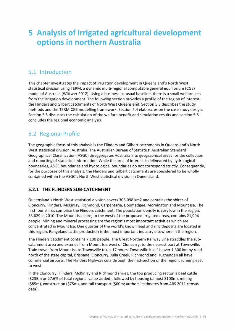
Chapter 5 Analysis of irrigated agricultural development options in northern Australia | 65
5 Analysis of irrigated agricultural development options in northern Australia
5.1 Introduction
This chapter investigates the impact of irrigation development in Queensland’s North West statistical division using TERM, a dynamic multi-regional computable general equilibrium (CGE) model of Australia (Wittwer 2012). Using a business-as-usual baseline, there is a small welfare loss from the irrigation development. The following section provides a profile of the region of interest- the Flinders and Gilbert catchments of North West Queensland. Section 5.3 describes the study methods and the TERM CGE modelling framework. Section 5.4 elaborates on the case study design. Section 5.5 discusses the calculation of the welfare benefit and simulation results and section 5.6 concludes the regional economic analysis.
5.2 Regional Profile
The geographic focus of this analysis is the Flinders and Gilbert catchments in Queensland’s North West statistical division, Australia. The Australian Bureau of Statistics’ Australian Standard Geographical Classification (ASGC) disaggregates Australia into geographical areas for the collection and reporting of statistical information. While the area of interest is delineated by hydrological boundaries, ASGC boundaries and hydrological boundaries do not correspond strictly. Consequently, for the purposes of this analysis, the Flinders and Gilbert catchments are considered to be wholly contained within the ASGC’s North West statistical division in Queensland.
5.2.1 THE FLINDERS SUB-CATCHMENT
Queensland’s North West statistical division covers 308,098 km2 and contains the shires of Cloncurry, Flinders, McKinlay, Richmond, Carpentaria, Doomadgee, Mornington and Mount Isa. The first four shires comprise the Flinders catchment. The population density is very low in the region: 33,629 in 2010. The Mount Isa shire, to the west of the proposed irrigated areas, contains 21,994 people. Mining and mineral processing are the region’s most important activities which are concentrated in Mount Isa. One quarter of the world’s known lead and zinc deposits are located in this region. Rangeland cattle production is the most important industry elsewhere in the region.
The Flinders catchment contains 7,100 people. The Great Northern Railway Line straddles the sub-catchment area and extends from Mount Isa, west of Cloncurry, to the nearest port at Townsville. Train travel from Mount Isa to Townsville takes 17 hours. Townsville itself is over 1,300 km by road north of the state capital, Brisbane. Cloncurry, Julia Creek, Richmond and Hughenden all have commercial airports. The Flinders Highway cuts through the mid-section of the region, running east to west.
In the Cloncurry, Flinders, McKinlay and Richmond shires, the top producing sector is beef cattle ($235m or 27.6% of total regional value-added), followed by housing (almost $100m), mining ($85m), construction ($75m), and rail transport ($60m; authors’ estimates from ABS 2011 census data).
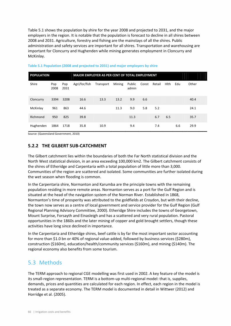
66 | Irrigation costs and benefits
Table 5.1 shows the population by shire for the year 2008 and projected to 2031, and the major employers in the region. It is notable that the population is forecast to decline in all shires between 2008 and 2031. Agriculture, forestry and fishing are the mainstays of all the shires. Public administration and safety services are important for all shires. Transportation and warehousing are important for Cloncurry and Hughenden while mining generates employment in Cloncurry and McKinlay.
Table 5.1 Population (2008 and projected to 2031) and major employers by shire
POPULATION MAJOR EMPLOYER AS PER CENT OF TOTAL EMPLOYMENT
Shire Pop 2008
Pop 2031
Agri/for/fish
Transport Mining Public admin
Const Retail Hlth Edu Other
Cloncurry 3394 3208 16.6 13.3 13.2 9.9 6.6 40.4
McKinlay 961 863 44.6 11.3 9.0 5.8 5.2 24.1
Richmond 950 825 39.8 11.3 6.7 6.5 35.7
Hughenden 1864 1718 35.8 10.9 9.4 7.4 6.6 29.9
Source: (Queensland Government, 2010)
5.2.2 THE GILBERT SUB-CATCHMENT
The Gilbert catchment lies within the boundaries of both the Far North statistical division and the North West statistical division, in an area exceeding 100,000 km2. The Gilbert catchment consists of the shires of Etheridge and Carpentaria with a total population of little more than 3,000. Communities of the region are scattered and isolated. Some communities are further isolated during the wet season when flooding is common.
In the Carpentaria shire, Normanton and Karumba are the principle towns with the remaining population residing in more remote areas. Normanton serves as a port for the Gulf Region and is situated at the head of the navigation system of the Norman River. Established in 1868, Normanton’s time of prosperity was attributed to the goldfields at Croydon, but with their decline, the town now serves as a centre of local government and service provider for the Gulf Region (Gulf Regional Planning Advisory Committee, 2000). Etheridge Shire includes the towns of Georgetown, Mount Surprise, Forsayth and Einasleigh and has a scattered and very rural population. Pastoral opportunities in the 1860s and the later mining of copper and gold brought settlers, though these activities have long since declined in importance.
In the Carpentaria and Etheridge shires, beef cattle is by far the most important sector accounting for more than $1.0 bn or 40% of regional value-added, followed by business services ($280m), construction ($160m), education/health/community services ($160m), and mining ($140m). The regional economy also benefits from some tourism.
5.3 Methods
The TERM approach to regional CGE modelling was first used in 2002. A key feature of the model is its small-region representation. TERM is a bottom-up multi-regional model: that is, supplies, demands, prices and quantities are calculated for each region. In effect, each region in the model is treated as a separate economy. The TERM model is documented in detail in Wittwer (2012) and Horridge et al. (2005).
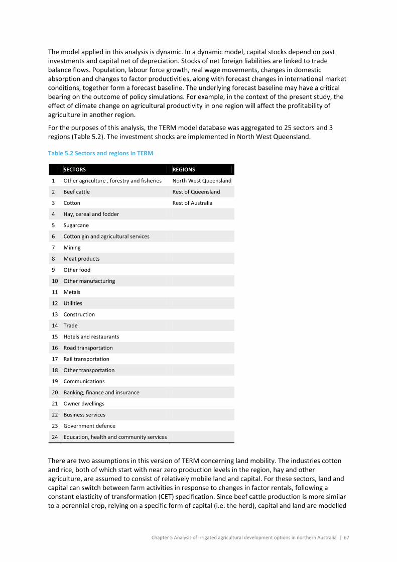
Chapter 5 Analysis of irrigated agricultural development options in northern Australia | 67
The model applied in this analysis is dynamic. In a dynamic model, capital stocks depend on past investments and capital net of depreciation. Stocks of net foreign liabilities are linked to trade balance flows. Population, labour force growth, real wage movements, changes in domestic absorption and changes to factor productivities, along with forecast changes in international market conditions, together form a forecast baseline. The underlying forecast baseline may have a critical bearing on the outcome of policy simulations. For example, in the context of the present study, the effect of climate change on agricultural productivity in one region will affect the profitability of agriculture in another region.
For the purposes of this analysis, the TERM model database was aggregated to 25 sectors and 3 regions (Table 5.2). The investment shocks are implemented in North West Queensland.
Table 5.2 Sectors and regions in TERM
SECTORS REGIONS
1 Other agriculture , forestry and fisheries North West Queensland
2 Beef cattle Rest of Queensland
3 Cotton Rest of Australia
4 Hay, cereal and fodder
5 Sugarcane
6 Cotton gin and agricultural services
7 Mining
8 Meat products
9 Other food
10 Other manufacturing
11 Metals
12 Utilities
13 Construction
14 Trade
15 Hotels and restaurants
16 Road transportation
17 Rail transportation
18 Other transportation
19 Communications
20 Banking, finance and insurance
21 Owner dwellings
22 Business services
23 Government defence
24 Education, health and community services
There are two assumptions in this version of TERM concerning land mobility. The industries cotton and rice, both of which start with near zero production levels in the region, hay and other agriculture, are assumed to consist of relatively mobile land and capital. For these sectors, land and capital can switch between farm activities in response to changes in factor rentals, following a constant elasticity of transformation (CET) specification. Since beef cattle production is more similar to a perennial crop, relying on a specific form of capital (i.e. the herd), capital and land are modelled
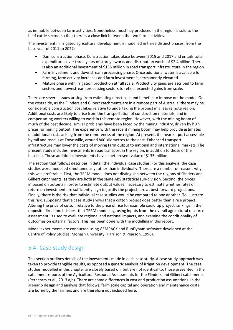
68 | Irrigation costs and benefits
as immobile between farm activities. Nonetheless, most hay produced in the region is sold to the beef cattle sector, so that there is a close link between the two farm activities.
The investment in irrigated agricultural development is modelled in three distinct phases, from the base year of 2011 to 2027:
• Dam construction phase. Construction takes place between 2015 and 2017 and entails total expenditures over three years of storage works and distribution works of $2.4 billion. There is also an additional investment of $135 million in road transport infrastructure in the region.
• Farm investment and downstream processing phase. Once additional water is available for farming, farm activity increases and farm investment is permanently elevated.
• Mature phase with irrigation production at full scale. Productivity gains are ascribed to farm sectors and downstream processing sectors to reflect expected gains from scale.
There are several issues arising from estimating direct cost and benefits to impose on the model. On the costs side, as the Flinders and Gilbert catchments are in a remote part of Australia, there may be considerable construction cost hikes relative to undertaking the project in a less remote region. Additional costs are likely to arise from the transportation of construction materials, and in compensating workers willing to work in this remote region. However, with the mining boom of much of the past decade, similar problems have been faced by the mining industry, driven by high prices for mining output. The experience with the recent mining boom may help provide estimates of additional costs arising from the remoteness of the region. At present, the nearest port accessible by rail and road is at Townsville, around 800 kilometres to the east. Enhanced transport infrastructure may lower the costs of moving farm output to national and international markets. The present study includes investments in road transport in the region, in addition to those of the baseline. These additional investments have a net present value of $135 million.
The section that follows describes in detail the individual case studies. For this analysis, the case studies were modelled simultaneously rather than individually. There are a number of reasons why this was preferable. First, the TERM model does not distinguish between the regions of Flinders and Gilbert catchments, as they are both in the same ABS statistical sub-division. Second, the prices imposed on outputs in order to estimate output values, necessary to estimate whether rates of return on investment are sufficiently high to justify the project, are at best forward projections. Finally, there is the risk that individual case studies would be compared to one another. To illustrate this risk, supposing that a case study shows that a cotton project does better than a rice project. Altering the price of cotton relative to the price of rice for example could tip project rankings in the opposite direction. It is best that TERM modelling, using inputs from the overall agricultural resource assessment, is used to evaluate regional and national impacts, and examine the conditionality of outcomes on external factors. This has been done with the modelling in this report.
Model experiments are conducted using GEMPACK and RunDynam software developed at the Centre of Policy Studies, Monash University (Harrison & Pearson, 1996).
5.4 Case study design
This section outlines details of the investments made in each case study. A case study approach was taken to provide tangible results, as opposed a generic analysis of irrigation development. The case studies modelled in this chapter are closely based on, but are not identical to, those presented in the catchment reports of the Agricultural Resource Assessments for the Flinders and Gilbert catchments (Petheram et al., 2013 a,b). There are some differences in cost and production assumptions. In the scenario design and analysis that follows, farm scale capital and operation and maintenance costs are borne by the farmers and are therefore not included here.
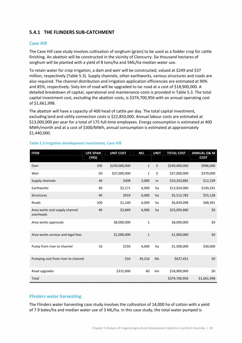
Chapter 5 Analysis of irrigated agricultural development options in northern Australia | 69
5.4.1 THE FLINDERS SUB-CATCHMENT
Cave Hill
The Cave Hill case study involves cultivation of sorghum (grain) to be used as a fodder crop for cattle finishing. An abattoir will be constructed in the vicinity of Cloncurry. Six thousand hectares of sorghum will be planted with a yield of 8 tons/ha and 5ML/ha median water use.
To retain water for crop irrigation, a dam and weir will be constructed, valued at $249 and $37 million, respectively (Table 5.3). Supply channels, other earthworks, various structures and roads are also required. The channel distribution and irrigation application efficiencies are estimated at 90% and 85%, respectively. Sixty km of road will be upgraded to tar road at a cost of $18,900,000. A detailed breakdown of capital, operational and maintenance costs is provided in Table 5.3. The total capital investment cost, excluding the abattoir costs, is $374,700,956 with an annual operating cost of $1,661,998.
The abattoir will have a capacity of 400 head of cattle per day. The total capital investment, excluding land and utility connection costs is $22,850,000. Annual labour costs are estimated at $13,000,000 per year for a total of 175 full-time employees. Energy consumption is estimated at 400 MWh/month and at a cost of $300/MWh, annual consumption is estimated at approximately $1,440,000.
Table 5.3 Irrigation development investment, Cave Hill
ITEM LIFE SPAN (YRS)
UNIT COST NO. UNIT TOTAL COST ANNUAL O& M COST
Dam 100 $249,000,000 1 $ $249,000,000 $996,000
Weir 50 $37,000,000 1 $ $37,000,000 $370,000
Supply channels 40 $408 3,000 m $10,203,885 $12,239
Earthworks 40 $2,171 6,000 ha $13,024,060 $130,241
Structures 40 $919 6,000 ha $5,512,782 $55,128
Roads 100 $1,140 6,000 ha $6,839,098 $68,391
Area works and supply channel overheads
40 $3,849 6,000 ha $23,093,680 $0
Area works approvals $8,000,000 1 $8,000,000 $0
Area works surveys and legal fees $1,000,000 1 $1,000,000 $0
Pump from river to channel 16 $250 6,000 ha $1,500,000 $30,000
Pumping cost from river to channel $16 39,216 ML $627,451 $0
Road upgrades $315,000 60 km $18,900,000 $0
Total $374,700,956 $1,661,998
Flinders water harvesting
The Flinders water harvesting case study involves the cultivation of 14,000 ha of cotton with a yield of 7.9 bales/ha and median water use of 3 ML/ha. In this case study, the total water pumped is
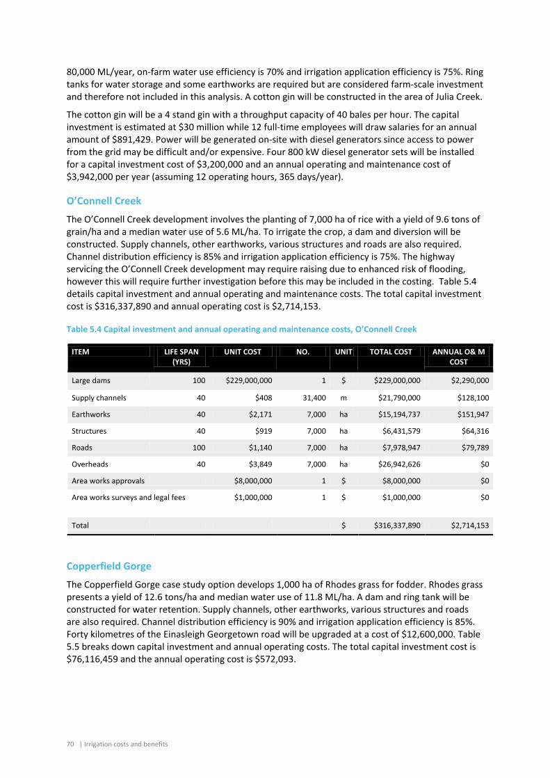
70 | Irrigation costs and benefits
80,000 ML/year, on-farm water use efficiency is 70% and irrigation application efficiency is 75%. Ring tanks for water storage and some earthworks are required but are considered farm-scale investment and therefore not included in this analysis. A cotton gin will be constructed in the area of Julia Creek.
The cotton gin will be a 4 stand gin with a throughput capacity of 40 bales per hour. The capital investment is estimated at $30 million while 12 full-time employees will draw salaries for an annual amount of $891,429. Power will be generated on-site with diesel generators since access to power from the grid may be difficult and/or expensive. Four 800 kW diesel generator sets will be installed for a capital investment cost of $3,200,000 and an annual operating and maintenance cost of $3,942,000 per year (assuming 12 operating hours, 365 days/year).
O’Connell Creek
The O’Connell Creek development involves the planting of 7,000 ha of rice with a yield of 9.6 tons of grain/ha and a median water use of 5.6 ML/ha. To irrigate the crop, a dam and diversion will be constructed. Supply channels, other earthworks, various structures and roads are also required. Channel distribution efficiency is 85% and irrigation application efficiency is 75%. The highway servicing the O’Connell Creek development may require raising due to enhanced risk of flooding, however this will require further investigation before this may be included in the costing. Table 5.4 details capital investment and annual operating and maintenance costs. The total capital investment cost is $316,337,890 and annual operating cost is $2,714,153.
Table 5.4 Capital investment and annual operating and maintenance costs, O’Connell Creek
ITEM LIFE SPAN (YRS)
UNIT COST NO. UNIT TOTAL COST ANNUAL O& M COST
Large dams 100 $229,000,000 1 $ $229,000,000 $2,290,000
Supply channels 40 $408 31,400 m $21,790,000 $128,100
Earthworks 40 $2,171 7,000 ha $15,194,737 $151,947
Structures 40 $919 7,000 ha $6,431,579 $64,316
Roads 100 $1,140 7,000 ha $7,978,947 $79,789
Overheads 40 $3,849 7,000 ha $26,942,626 $0
Area works approvals $8,000,000 1 $ $8,000,000 $0
Area works surveys and legal fees $1,000,000 1 $ $1,000,000 $0
Total $ $316,337,890 $2,714,153
Copperfield Gorge
The Copperfield Gorge case study option develops 1,000 ha of Rhodes grass for fodder. Rhodes grass presents a yield of 12.6 tons/ha and median water use of 11.8 ML/ha. A dam and ring tank will be constructed for water retention. Supply channels, other earthworks, various structures and roads are also required. Channel distribution efficiency is 90% and irrigation application efficiency is 85%. Forty kilometres of the Einasleigh Georgetown road will be upgraded at a cost of $12,600,000. Table 5.5 breaks down capital investment and annual operating costs. The total capital investment cost is $76,116,459 and the annual operating cost is $572,093.
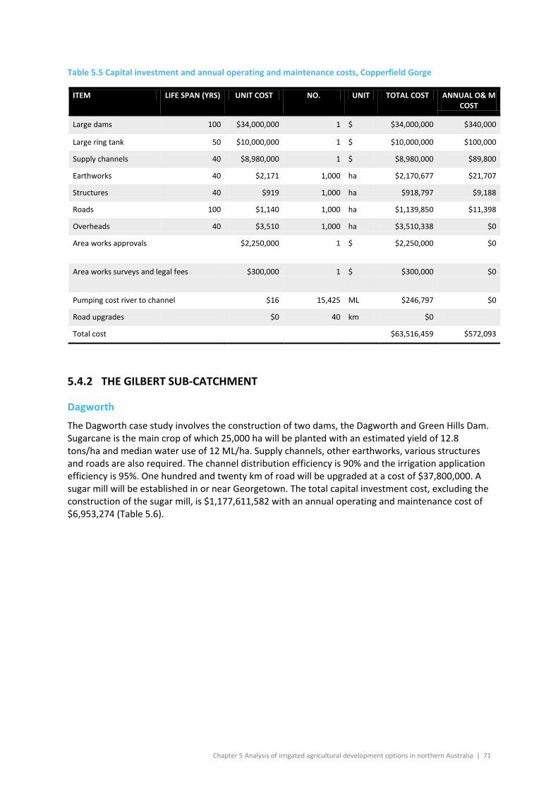
Chapter 5 Analysis of irrigated agricultural development options in northern Australia | 71
Table 5.5 Capital investment and annual operating and maintenance costs, Copperfield Gorge
ITEM LIFE SPAN (YRS) UNIT COST NO. UNIT TOTAL COST ANNUAL O& M COST
Large dams 100 $34,000,000 1 $ $34,000,000 $340,000
Large ring tank 50 $10,000,000 1 $ $10,000,000 $100,000
Supply channels 40 $8,980,000 1 $ $8,980,000 $89,800
Earthworks 40 $2,171 1,000 ha $2,170,677 $21,707
Structures 40 $919 1,000 ha $918,797 $9,188
Roads 100 $1,140 1,000 ha $1,139,850 $11,398
Overheads 40 $3,510 1,000 ha $3,510,338 $0
Area works approvals $2,250,000 1 $ $2,250,000 $0
Area works surveys and legal fees $300,000 1 $ $300,000 $0
Pumping cost river to channel $16 15,425 ML $246,797 $0
Road upgrades $0 40 km $0
Total cost $63,516,459 $572,093
5.4.2 THE GILBERT SUB-CATCHMENT
Dagworth
The Dagworth case study involves the construction of two dams, the Dagworth and Green Hills Dam. Sugarcane is the main crop of which 25,000 ha will be planted with an estimated yield of 12.8 tons/ha and median water use of 12 ML/ha. Supply channels, other earthworks, various structures and roads are also required. The channel distribution efficiency is 90% and the irrigation application efficiency is 95%. One hundred and twenty km of road will be upgraded at a cost of $37,800,000. A sugar mill will be established in or near Georgetown. The total capital investment cost, excluding the construction of the sugar mill, is $1,177,611,582 with an annual operating and maintenance cost of $6,953,274 (Table 5.6).
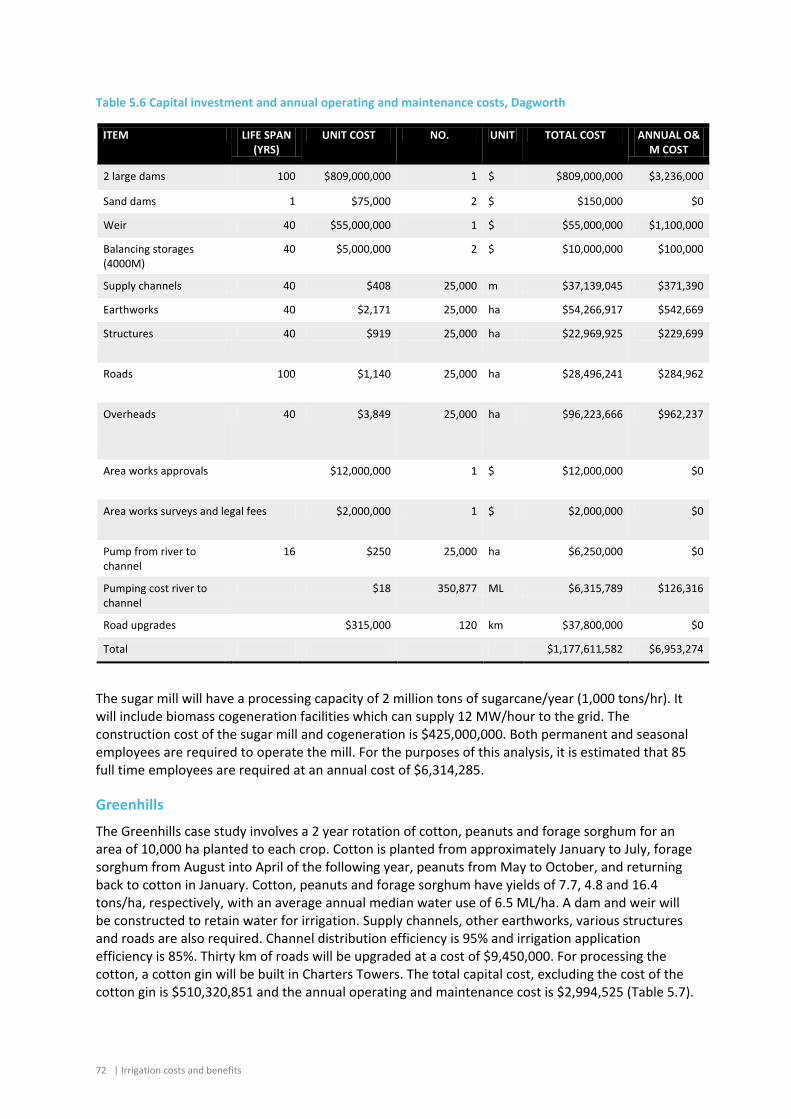
72 | Irrigation costs and benefits
Table 5.6 Capital investment and annual operating and maintenance costs, Dagworth
ITEM LIFE SPAN (YRS)
UNIT COST NO. UNIT TOTAL COST ANNUAL O& M COST
2 large dams 100 $809,000,000 1 $ $809,000,000 $3,236,000
Sand dams 1 $75,000 2 $ $150,000 $0
Weir 40 $55,000,000 1 $ $55,000,000 $1,100,000
Balancing storages (4000M)
40 $5,000,000 2 $ $10,000,000 $100,000
Supply channels 40 $408 25,000 m $37,139,045 $371,390
Earthworks 40 $2,171 25,000 ha $54,266,917 $542,669
Structures 40 $919 25,000 ha $22,969,925 $229,699
Roads 100 $1,140 25,000 ha $28,496,241 $284,962
Overheads 40 $3,849 25,000 ha $96,223,666 $962,237
Area works approvals $12,000,000 1 $ $12,000,000 $0
Area works surveys and legal fees $2,000,000 1 $ $2,000,000 $0
Pump from river to channel
16 $250 25,000 ha $6,250,000 $0
Pumping cost river to channel
$18 350,877 ML $6,315,789 $126,316
Road upgrades $315,000 120 km $37,800,000 $0
Total $1,177,611,582 $6,953,274
The sugar mill will have a processing capacity of 2 million tons of sugarcane/year (1,000 tons/hr). It will include biomass cogeneration facilities which can supply 12 MW/hour to the grid. The construction cost of the sugar mill and cogeneration is $425,000,000. Both permanent and seasonal employees are required to operate the mill. For the purposes of this analysis, it is estimated that 85 full time employees are required at an annual cost of $6,314,285.
Greenhills
The Greenhills case study involves a 2 year rotation of cotton, peanuts and forage sorghum for an area of 10,000 ha planted to each crop. Cotton is planted from approximately January to July, forage sorghum from August into April of the following year, peanuts from May to October, and returning back to cotton in January. Cotton, peanuts and forage sorghum have yields of 7.7, 4.8 and 16.4 tons/ha, respectively, with an average annual median water use of 6.5 ML/ha. A dam and weir will be constructed to retain water for irrigation. Supply channels, other earthworks, various structures and roads are also required. Channel distribution efficiency is 95% and irrigation application efficiency is 85%. Thirty km of roads will be upgraded at a cost of $9,450,000. For processing the cotton, a cotton gin will be built in Charters Towers. The total capital cost, excluding the cost of the cotton gin is $510,320,851 and the annual operating and maintenance cost is $2,994,525 (Table 5.7).
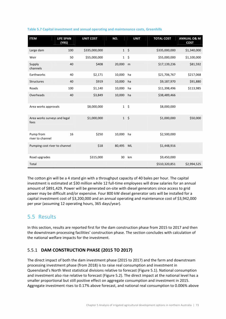
Chapter 5 Analysis of irrigated agricultural development options in northern Australia | 73
Table 5.7 Capital investment and annual operating and maintenance costs, Greenhills
ITEM LIFE SPAN (YRS)
UNIT COST NO. UNIT TOTAL COST ANNUAL O& M COST
Large dam 100 $335,000,000 1 $ $335,000,000 $1,340,000
Weir 50 $55,000,000 1 $ $55,000,000 $1,100,000
Supply channels
40 $408 20,000 m $17,139,236 $81,592
Earthworks 40 $2,171 10,000 ha $21,706,767 $217,068
Structures 40 $919 10,000 ha $9,187,970 $91,880
Roads 100 $1,140 10,000 ha $11,398,496 $113,985
Overheads 40 $3,849 10,000 ha $38,489,466
Area works approvals $8,000,000 1 $ $8,000,000
Area works surveys and legal fees
$1,000,000 1 $ $1,000,000 $50,000
Pump from river to channel
16 $250 10,000 ha $2,500,000
Pumping cost river to channel $18 80,495 ML $1,448,916
Road upgrades $315,000 30 km $9,450,000
Total $510,320,851 $2,994,525
The cotton gin will be a 4 stand gin with a throughput capacity of 40 bales per hour. The capital investment is estimated at $30 million while 12 full-time employees will draw salaries for an annual amount of $891,429. Power will be generated on-site with diesel generators since access to grid power may be difficult and/or expensive. Four 800 kW diesel generator sets will be installed for a capital investment cost of $3,200,000 and an annual operating and maintenance cost of $3,942,000 per year (assuming 12 operating hours, 365 days/year).
5.5 Results
In this section, results are reported first for the dam construction phase from 2015 to 2017 and then the downstream processing facilities’ construction phase. The section concludes with calculation of the national welfare impacts for the investment.
5.5.1 DAM CONSTRUCTION PHASE (2015 TO 2017)
The direct impact of both the dam investment phase (2015 to 2017) and the farm and downstream processing investment phase (from 2018) is to raise real consumption and investment in Queensland’s North West statistical divisions relative to forecast (Figure 5.1). National consumption and investment also rise relative to forecast (Figure 5.2). The direct impact at the national level has a smaller proportional but still positive effect on aggregate consumption and investment in 2015. Aggregate investment rises to 0.17% above forecast, and national real consumption to 0.006% above
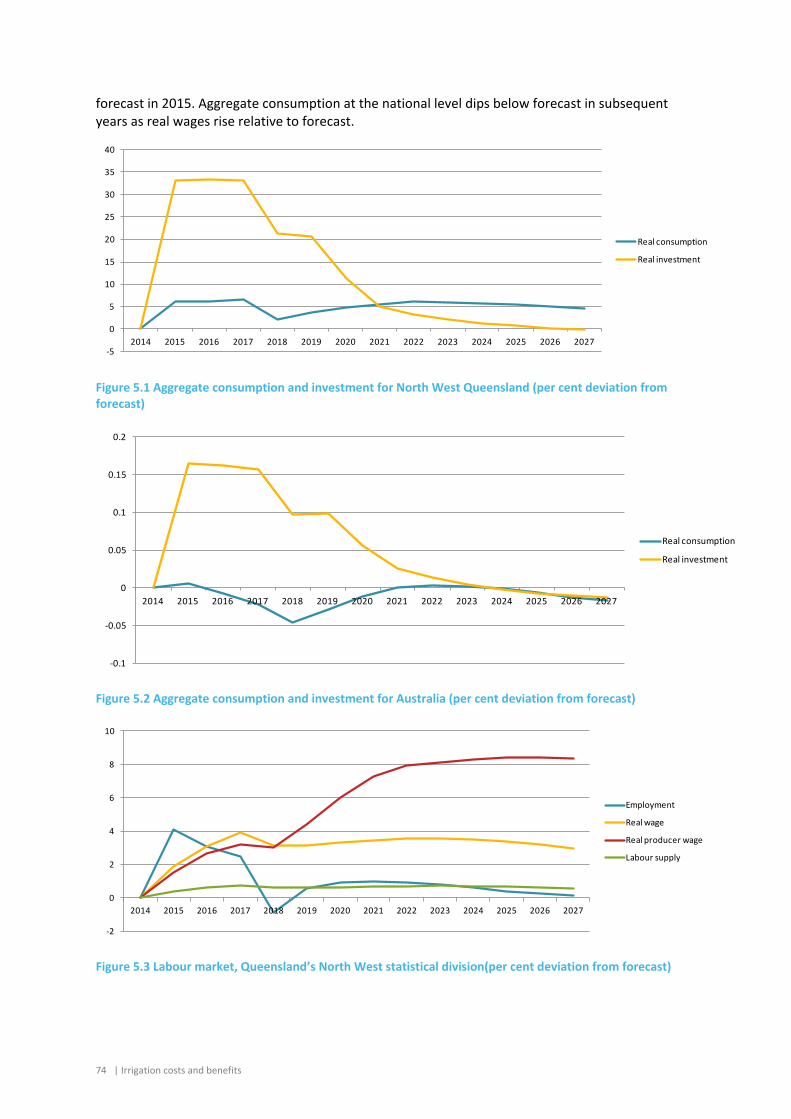
74 | Irrigation costs and benefits
forecast in 2015. Aggregate consumption at the national level dips below forecast in subsequent years as real wages rise relative to forecast.
Figure 5.1 Aggregate consumption and investment for North West Queensland (per cent deviation from forecast)
Figure 5.2 Aggregate consumption and investment for Australia (per cent deviation from forecast)
Figure 5.3 Labour market, Queensland’s North West statistical division(per cent deviation from forecast)
-5
0
5
10
15
20
25
30
35
40
2014 2015 2016 2017 2018 2019 2020 2021 2022 2023 2024 2025 2026 2027
Real consumption
Real investment
-0.1
-0.05
0
0.05
0.1
0.15
0.2
2014 2015 2016 2017 2018 2019 2020 2021 2022 2023 2024 2025 2026 2027
Real consumption
Real investment
-2
0
2
4
6
8
10
2014 2015 2016 2017 2018 2019 2020 2021 2022 2023 2024 2025 2026 2027
Employment
Real wage
Real producer wage
Labour supply
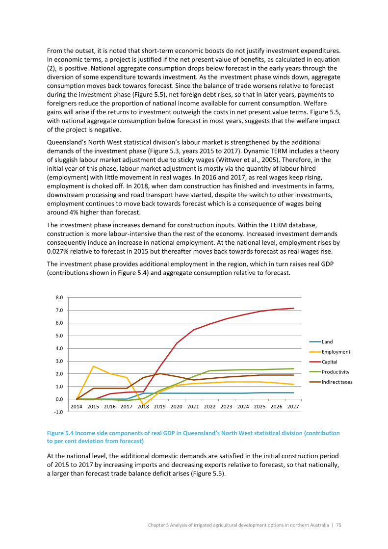
Chapter 5 Analysis of irrigated agricultural development options in northern Australia | 75
From the outset, it is noted that short-term economic boosts do not justify investment expenditures. In economic terms, a project is justified if the net present value of benefits, as calculated in equation (2), is positive. National aggregate consumption drops below forecast in the early years through the diversion of some expenditure towards investment. As the investment phase winds down, aggregate consumption moves back towards forecast. Since the balance of trade worsens relative to forecast during the investment phase (Figure 5.5), net foreign debt rises, so that in later years, payments to foreigners reduce the proportion of national income available for current consumption. Welfare gains will arise if the returns to investment outweigh the costs in net present value terms. Figure 5.5, with national aggregate consumption below forecast in most years, suggests that the welfare impact of the project is negative.
Queensland’s North West statistical division’s labour market is strengthened by the additional demands of the investment phase (Figure 5.3, years 2015 to 2017). Dynamic TERM includes a theory of sluggish labour market adjustment due to sticky wages (Wittwer et al., 2005). Therefore, in the initial year of this phase, labour market adjustment is mostly via the quantity of labour hired (employment) with little movement in real wages. In 2016 and 2017, as real wages keep rising, employment is choked off. In 2018, when dam construction has finished and investments in farms, downstream processing and road transport have started, despite the switch to other investments, employment continues to move back towards forecast which is a consequence of wages being around 4% higher than forecast.
The investment phase increases demand for construction inputs. Within the TERM database, construction is more labour-intensive than the rest of the economy. Increased investment demands consequently induce an increase in national employment. At the national level, employment rises by 0.027% relative to forecast in 2015 but thereafter moves back towards forecast as real wages rise.
The investment phase provides additional employment in the region, which in turn raises real GDP (contributions shown in Figure 5.4) and aggregate consumption relative to forecast.
Figure 5.4 Income side components of real GDP in Queensland’s North West statistical division (contribution to per cent deviation from forecast)
At the national level, the additional domestic demands are satisfied in the initial construction period of 2015 to 2017 by increasing imports and decreasing exports relative to forecast, so that nationally, a larger than forecast trade balance deficit arises (Figure 5.5).
-1.0
0.0
1.0
2.0
3.0
4.0
5.0
6.0
7.0
8.0
2014 2015 2016 2017 2018 2019 2020 2021 2022 2023 2024 2025 2026 2027
Land
Employment
Capital
Productivity
Indirect taxes
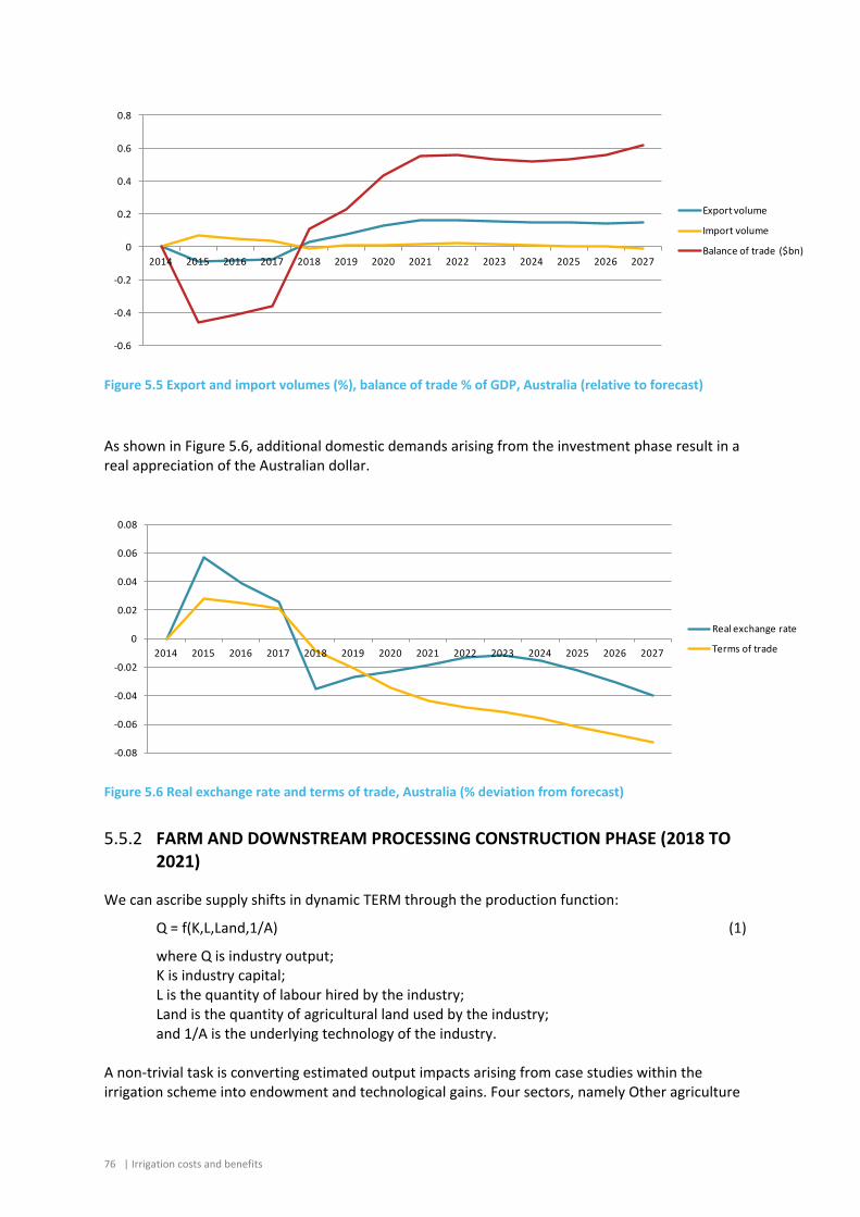
76 | Irrigation costs and benefits
Figure 5.5 Export and import volumes (%), balance of trade % of GDP, Australia (relative to forecast)
As shown in Figure 5.6, additional domestic demands arising from the investment phase result in a real appreciation of the Australian dollar.
Figure 5.6 Real exchange rate and terms of trade, Australia (% deviation from forecast)
5.5.2 FARM AND DOWNSTREAM PROCESSING CONSTRUCTION PHASE (2018 TO 2021)
We can ascribe supply shifts in dynamic TERM through the production function:
Q = f(K,L,Land,1/A) (1)
where Q is industry output; K is industry capital; L is the quantity of labour hired by the industry; Land is the quantity of agricultural land used by the industry; and 1/A is the underlying technology of the industry.
A non-trivial task is converting estimated output impacts arising from case studies within the irrigation scheme into endowment and technological gains. Four sectors, namely Other agriculture
-0.6
-0.4
-0.2
0
0.2
0.4
0.6
0.8
2014 2015 2016 2017 2018 2019 2020 2021 2022 2023 2024 2025 2026 2027
Export volume
Import volume
Balance of trade ($bn)
-0.08
-0.06
-0.04
-0.02
0
0.02
0.04
0.06
0.08
2014 2015 2016 2017 2018 2019 2020 2021 2022 2023 2024 2025 2026 2027
Real exchange rate
Terms of trade
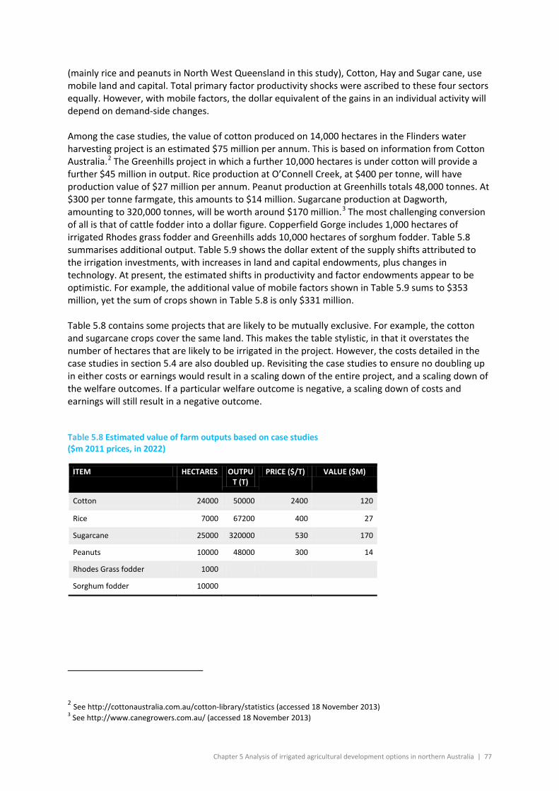
Chapter 5 Analysis of irrigated agricultural development options in northern Australia | 77
(mainly rice and peanuts in North West Queensland in this study), Cotton, Hay and Sugar cane, use mobile land and capital. Total primary factor productivity shocks were ascribed to these four sectors equally. However, with mobile factors, the dollar equivalent of the gains in an individual activity will depend on demand-side changes. Among the case studies, the value of cotton produced on 14,000 hectares in the Flinders water harvesting project is an estimated $75 million per annum. This is based on information from Cotton Australia.2 The Greenhills project in which a further 10,000 hectares is under cotton will provide a further $45 million in output. Rice production at O’Connell Creek, at $400 per tonne, will have production value of $27 million per annum. Peanut production at Greenhills totals 48,000 tonnes. At $300 per tonne farmgate, this amounts to $14 million. Sugarcane production at Dagworth, amounting to 320,000 tonnes, will be worth around $170 million.3 The most challenging conversion of all is that of cattle fodder into a dollar figure. Copperfield Gorge includes 1,000 hectares of irrigated Rhodes grass fodder and Greenhills adds 10,000 hectares of sorghum fodder. Table 5.8 summarises additional output. Table 5.9 shows the dollar extent of the supply shifts attributed to the irrigation investments, with increases in land and capital endowments, plus changes in technology. At present, the estimated shifts in productivity and factor endowments appear to be optimistic. For example, the additional value of mobile factors shown in Table 5.9 sums to $353 million, yet the sum of crops shown in Table 5.8 is only $331 million. Table 5.8 contains some projects that are likely to be mutually exclusive. For example, the cotton and sugarcane crops cover the same land. This makes the table stylistic, in that it overstates the number of hectares that are likely to be irrigated in the project. However, the costs detailed in the case studies in section 5.4 are also doubled up. Revisiting the case studies to ensure no doubling up in either costs or earnings would result in a scaling down of the entire project, and a scaling down of the welfare outcomes. If a particular welfare outcome is negative, a scaling down of costs and earnings will still result in a negative outcome.
Table 5.8 Estimated value of farm outputs based on case studies ($m 2011 prices, in 2022)
ITEM HECTARES OUTPUT (T)
PRICE ($/T) VALUE ($M)
Cotton 24000 50000 2400 120
Rice 7000 67200 400 27
Sugarcane 25000 320000 530 170
Peanuts 10000 48000 300 14
Rhodes Grass fodder 1000
Sorghum fodder 10000
2 See http://cottonaustralia.com.au/cotton-library/statistics (accessed 18 November 2013) 3 See http://www.canegrowers.com.au/ (accessed 18 November 2013)
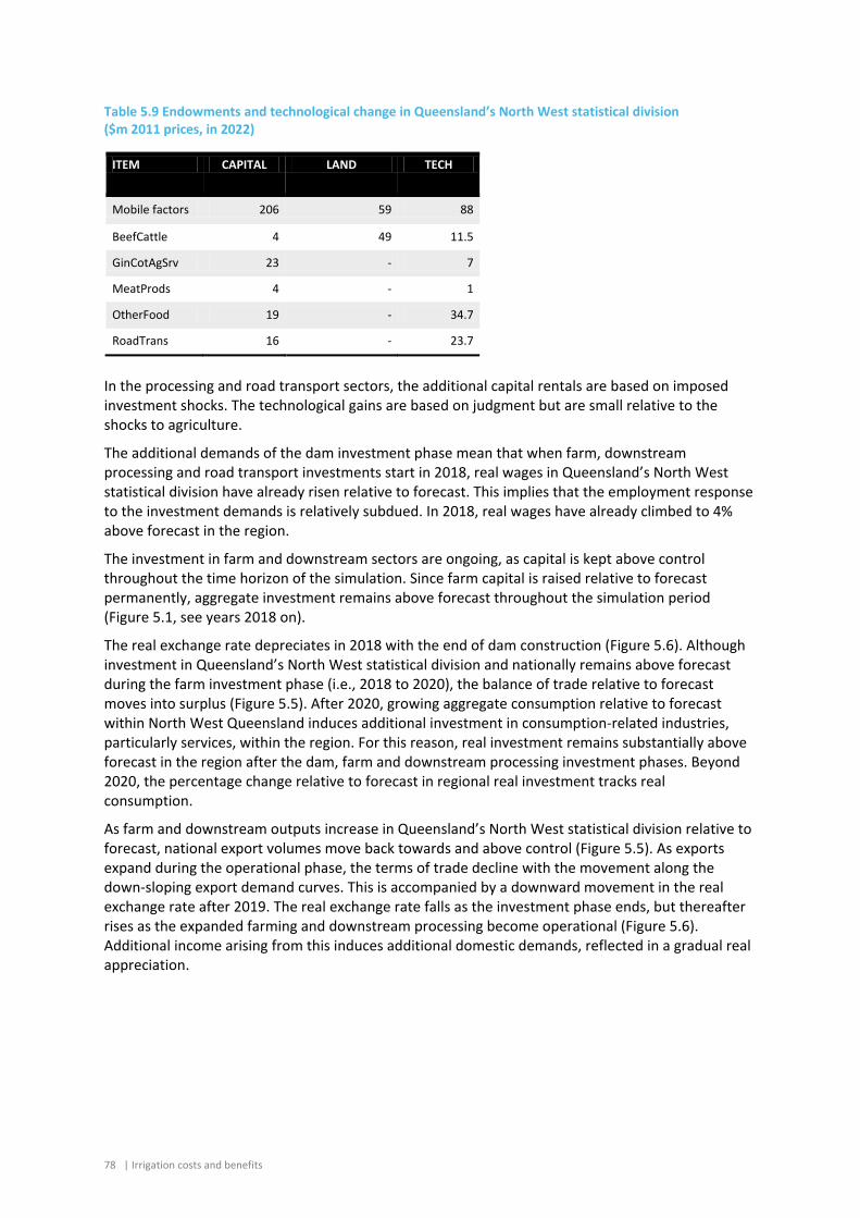
78 | Irrigation costs and benefits
Table 5.9 Endowments and technological change in Queensland’s North West statistical division ($m 2011 prices, in 2022)
ITEM CAPITAL LAND TECH
Mobile factors 206 59 88
BeefCattle 4 49 11.5
GinCotAgSrv 23 - 7
MeatProds 4 - 1
OtherFood 19 - 34.7
RoadTrans 16 - 23.7
In the processing and road transport sectors, the additional capital rentals are based on imposed investment shocks. The technological gains are based on judgment but are small relative to the shocks to agriculture.
The additional demands of the dam investment phase mean that when farm, downstream processing and road transport investments start in 2018, real wages in Queensland’s North West statistical division have already risen relative to forecast. This implies that the employment response to the investment demands is relatively subdued. In 2018, real wages have already climbed to 4% above forecast in the region.
The investment in farm and downstream sectors are ongoing, as capital is kept above control throughout the time horizon of the simulation. Since farm capital is raised relative to forecast permanently, aggregate investment remains above forecast throughout the simulation period (Figure 5.1, see years 2018 on).
The real exchange rate depreciates in 2018 with the end of dam construction (Figure 5.6). Although investment in Queensland’s North West statistical division and nationally remains above forecast during the farm investment phase (i.e., 2018 to 2020), the balance of trade relative to forecast moves into surplus (Figure 5.5). After 2020, growing aggregate consumption relative to forecast within North West Queensland induces additional investment in consumption-related industries, particularly services, within the region. For this reason, real investment remains substantially above forecast in the region after the dam, farm and downstream processing investment phases. Beyond 2020, the percentage change relative to forecast in regional real investment tracks real consumption.
As farm and downstream outputs increase in Queensland’s North West statistical division relative to forecast, national export volumes move back towards and above control (Figure 5.5). As exports expand during the operational phase, the terms of trade decline with the movement along the down-sloping export demand curves. This is accompanied by a downward movement in the real exchange rate after 2019. The real exchange rate falls as the investment phase ends, but thereafter rises as the expanded farming and downstream processing become operational (Figure 5.6). Additional income arising from this induces additional domestic demands, reflected in a gradual real appreciation.
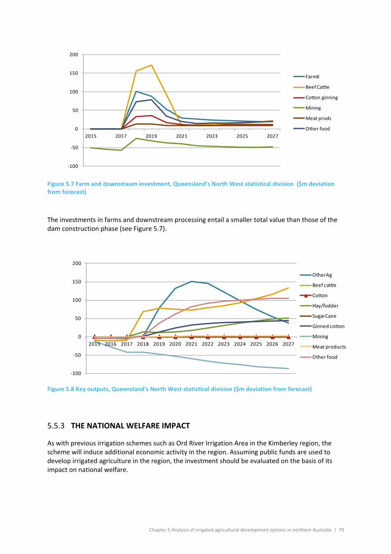
Chapter 5 Analysis of irrigated agricultural development options in northern Australia | 79
Figure 5.7 Farm and downstream investment, Queensland’s North West statistical division ($m deviation from forecast)
The investments in farms and downstream processing entail a smaller total value than those of the dam construction phase (see Figure 5.7).
Figure 5.8 Key outputs, Queensland’s North West statistical division ($m deviation from forecast)
5.5.3 THE NATIONAL WELFARE IMPACT
As with previous irrigation schemes such as Ord River Irrigation Area in the Kimberley region, the scheme will induce additional economic activity in the region. Assuming public funds are used to develop irrigated agriculture in the region, the investment should be evaluated on the basis of its impact on national welfare.
-100
-50
0
50
100
150
200
2015 2017 2019 2021 2023 2025 2027
FarmK
Beef Cattle
Cotton ginning
Mining
Meat prods
Other food
-100
-50
0
50
100
150
200
2015 2016 2017 2018 2019 2020 2021 2022 2023 2024 2025 2026 2027
OtherAg
Beef cattle
Cotton
Hay/fodder
SugarCane
Ginned cotton
Mining
Meat products
Other food
80 | Irrigation costs and benefits
Welfare (dWELF) is calculated at the national level:
dCON dGOV dNFLdWELF1 1t z
d t
( d ,t ) ( d ,t ) ( z )( r ) ( r )
+= −
− −∑∑ (2)
where dCON and dGOV are the deviations in real household and government spending in region d and year t; dNFL is the deviation in real net foreign liabilities in the final year (z) of the simulation; and r is the discount rate. One complication in equation (3) is that the deviation in current consumption is not near zero by 2027. The simulation was projected further out to 2035, by which time the deviation was still below zero and moving back towards zero. The welfare impact of the final year z was calculated as
n x [dCON(d,z)+dGOV(I)]/(1-r)z (3)
where n = 0.5. If the deviation were not trending gradually towards control but instead were constant, n would be set at 1.0.
The above equations provide a lifetime estimate of the welfare impact. We can pare this back to an annualised welfare figure by multiplying the welfare impact by the discount rate. An annualised figure enables us to compare the welfare outcome with annual figures such as are shown in Table 5.8 and Table 5.9.This provides an opportunity to explore the conditionality of welfare impacts on baseline economic conditions. The net present value of the annualised welfare impact is minus $69 million. That is, despite the use of what appear to very optimistic productivity and endowment projects, as is apparent from comparing Table 5.8 with Table 5.9, the project results in a welfare loss.
Another dimension of conditionality concerns the discount rate. Long term projects are more readily justified if the discount rate is lower. A discount rate of 5% is used in this study. As the discount rate falls, returns in later years have a higher weighting in the welfare calculation. Over a long period of time, it may be difficult to justify a lower discount rate than that used in this study, given that Australia’s interest rates are currently at 50 year lows. A lower discount raised is used in this chapter than elsewhere in the study. This also makes a contribution to modelled outcomes that appear more favourable than elsewhere in other chapters this study, though the supply shift is the main driver.
5.6 Conclusions
Better estimates of construction and operational costs, and of the composition and volume of increased farm outputs will refine the estimates of the net benefits of the proposed scheme. Further work on estimating the links between climate change and farm productivity will enrich this study. Since the model includes year-by-year dynamics, there is no need to restrict further analysis to “typical year” studies. If an implication of climate change is that seasons and yields in southern Australia become more erratic, such variations across years can be included in the baseline. Furthermore, transport is a significant component of costs of production in a region as remote as North West Queensland. As such, the costs of transporting products within and between regions ought to be examined more carefully. A logistical study on transport options may be an important component in the evaluation of this type of investment.
Chapter 6 Evaluating the logistics costs from new or modified supply chains | 81
6 Evaluating the logistics costs from new or modified supply chains
6.1 Introduction
This chapter aims to identify transport cost savings by locating a potential abattoir, sugar mill and cotton gin closer to the Flinders and Gilbert catchments than the location of the nearest existing facilities, which are located long distances from the catchments. The analysis in this chapter has two main purposes: i) to identify potential costs savings that may be available to producers who would incur high transport costs should they invest in irrigation, and; ii) provide information for the case studies reported in the Flinders and Gilbert Agricultural Resource Assessment Catchment Reports (see Petheram et al., 2013a,b).
6.2 Objectives and scope
This chapter relates to three case studies considered by the Assessment:
• A potential irrigation development near Cloncurry was investigated. The development would enable sorghum (grain) to be supplied to a newly established local feedlot and abattoir facilities to grow the regional beef industry. Irrigation water would be supplied from a dam built at Cave Hill. For livestock, this would alter supply chain paths as cattle, originally going to live export out of Darwin or east-coast abattoirs, would now be fattened in the Flinders and processed at a new abattoir at Cloncurry. For each of these scenarios, transport costs and traffic flows are estimated in the context of the existing road network and vehicle configuration requirements.
• A potential irrigation development along the Gilbert River was investigated. The development is based on a crop rotation of cotton, peanuts and an irrigated fodder, with a new cotton gin. The nearest gin is at Emerald. A scenario was tested involving a new gin located at Charters Towers.
• A potential two dam-irrigation development on the Gilbert and Einasleigh rivers was investigated, both as a pair and singly. The development under consideration would enable sugarcane to be supplied to a newly established sugar mill in the Gilbert catchment. Irrigation water would be supplied from dams built at one or both of Green Hills and Dagworth stations.
In a “Livestock Logistics” project funded by the Office of Northern Australia and state governments, a set of logistics tools were developed to evaluate transport costs for modified supply chains and infrastructure investments in the northern beef industry (Higgins et al 2013). In this FGARA project we apply one of these tools, the Strategic Transport Simulation Model, to estimate transport costs and flows.
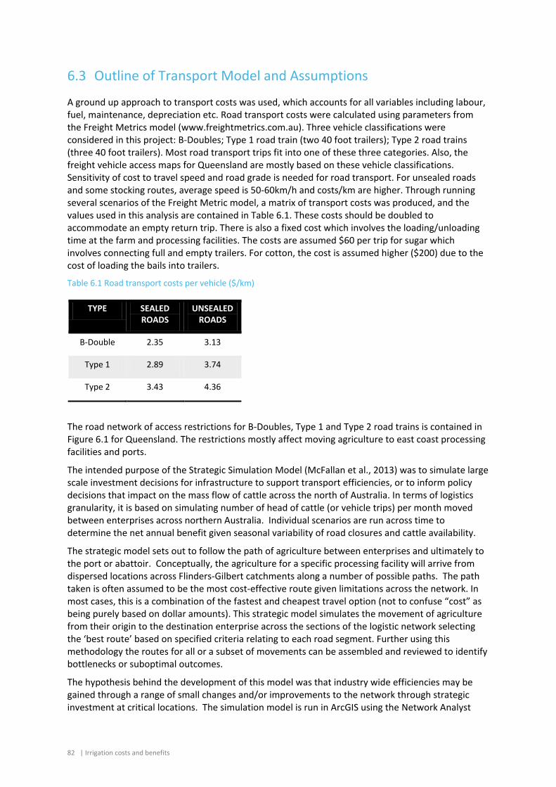
82 | Irrigation costs and benefits
6.3 Outline of Transport Model and Assumptions
A ground up approach to transport costs was used, which accounts for all variables including labour, fuel, maintenance, depreciation etc. Road transport costs were calculated using parameters from the Freight Metrics model (www.freightmetrics.com.au). Three vehicle classifications were considered in this project: B-Doubles; Type 1 road train (two 40 foot trailers); Type 2 road trains (three 40 foot trailers). Most road transport trips fit into one of these three categories. Also, the freight vehicle access maps for Queensland are mostly based on these vehicle classifications. Sensitivity of cost to travel speed and road grade is needed for road transport. For unsealed roads and some stocking routes, average speed is 50-60km/h and costs/km are higher. Through running several scenarios of the Freight Metric model, a matrix of transport costs was produced, and the values used in this analysis are contained in Table 6.1. These costs should be doubled to accommodate an empty return trip. There is also a fixed cost which involves the loading/unloading time at the farm and processing facilities. The costs are assumed $60 per trip for sugar which involves connecting full and empty trailers. For cotton, the cost is assumed higher ($200) due to the cost of loading the bails into trailers.
Table 6.1 Road transport costs per vehicle ($/km)
TYPE SEALED ROADS
UNSEALED ROADS
B-Double 2.35 3.13
Type 1 2.89 3.74
Type 2 3.43 4.36
The road network of access restrictions for B-Doubles, Type 1 and Type 2 road trains is contained in Figure 6.1 for Queensland. The restrictions mostly affect moving agriculture to east coast processing facilities and ports.
The intended purpose of the Strategic Simulation Model (McFallan et al., 2013) was to simulate large scale investment decisions for infrastructure to support transport efficiencies, or to inform policy decisions that impact on the mass flow of cattle across the north of Australia. In terms of logistics granularity, it is based on simulating number of head of cattle (or vehicle trips) per month moved between enterprises across northern Australia. Individual scenarios are run across time to determine the net annual benefit given seasonal variability of road closures and cattle availability.
The strategic model sets out to follow the path of agriculture between enterprises and ultimately to the port or abattoir. Conceptually, the agriculture for a specific processing facility will arrive from dispersed locations across Flinders-Gilbert catchments along a number of possible paths. The path taken is often assumed to be the most cost-effective route given limitations across the network. In most cases, this is a combination of the fastest and cheapest travel option (not to confuse “cost” as being purely based on dollar amounts). This strategic model simulates the movement of agriculture from their origin to the destination enterprise across the sections of the logistic network selecting the ‘best route’ based on specified criteria relating to each road segment. Further using this methodology the routes for all or a subset of movements can be assembled and reviewed to identify bottlenecks or suboptimal outcomes.
The hypothesis behind the development of this model was that industry wide efficiencies may be gained through a range of small changes and/or improvements to the network through strategic investment at critical locations. The simulation model is run in ArcGIS using the Network Analyst
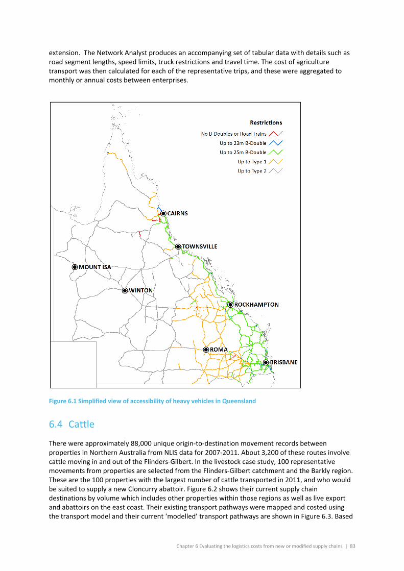
Chapter 6 Evaluating the logistics costs from new or modified supply chains | 83
extension. The Network Analyst produces an accompanying set of tabular data with details such as road segment lengths, speed limits, truck restrictions and travel time. The cost of agriculture transport was then calculated for each of the representative trips, and these were aggregated to monthly or annual costs between enterprises.
Figure 6.1 Simplified view of accessibility of heavy vehicles in Queensland
6.4 Cattle
There were approximately 88,000 unique origin-to-destination movement records between properties in Northern Australia from NLIS data for 2007-2011. About 3,200 of these routes involve cattle moving in and out of the Flinders-Gilbert. In the livestock case study, 100 representative movements from properties are selected from the Flinders-Gilbert catchment and the Barkly region. These are the 100 properties with the largest number of cattle transported in 2011, and who would be suited to supply a new Cloncurry abattoir. Figure 6.2 shows their current supply chain destinations by volume which includes other properties within those regions as well as live export and abattoirs on the east coast. Their existing transport pathways were mapped and costed using the transport model and their current ‘modelled’ transport pathways are shown in Figure 6.3. Based
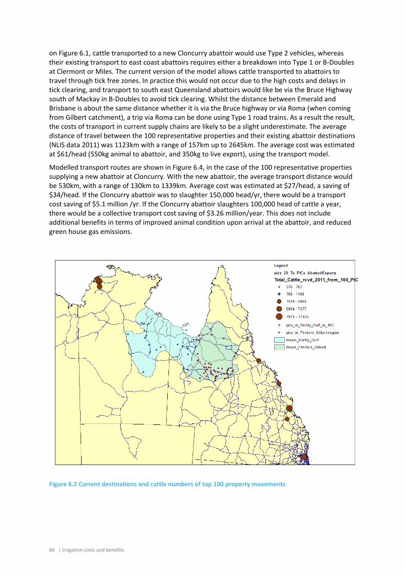
84 | Irrigation costs and benefits
on Figure 6.1, cattle transported to a new Cloncurry abattoir would use Type 2 vehicles, whereas their existing transport to east coast abattoirs requires either a breakdown into Type 1 or B-Doubles at Clermont or Miles. The current version of the model allows cattle transported to abattoirs to travel through tick free zones. In practice this would not occur due to the high costs and delays in tick clearing, and transport to south east Queensland abattoirs would like be via the Bruce Highway south of Mackay in B-Doubles to avoid tick clearing. Whilst the distance between Emerald and Brisbane is about the same distance whether it is via the Bruce highway or via Roma (when coming from Gilbert catchment), a trip via Roma can be done using Type 1 road trains. As a result the result, the costs of transport in current supply chains are likely to be a slight underestimate. The average distance of travel between the 100 representative properties and their existing abattoir destinations (NLIS data 2011) was 1123km with a range of 157km up to 2645km. The average cost was estimated at $61/head (550kg animal to abattoir, and 350kg to live export), using the transport model.
Modelled transport routes are shown in Figure 6.4, in the case of the 100 representative properties supplying a new abattoir at Cloncurry. With the new abattoir, the average transport distance would be 530km, with a range of 130km to 1339km. Average cost was estimated at $27/head, a saving of $34/head. If the Cloncurry abattoir was to slaughter 150,000 head/yr, there would be a transport cost saving of $5.1 million /yr. If the Cloncurry abattoir slaughters 100,000 head of cattle a year, there would be a collective transport cost saving of $3.26 million/year. This does not include additional benefits in terms of improved animal condition upon arrival at the abattoir, and reduced green house gas emissions.
Figure 6.2 Current destinations and cattle numbers of top 100 property movements
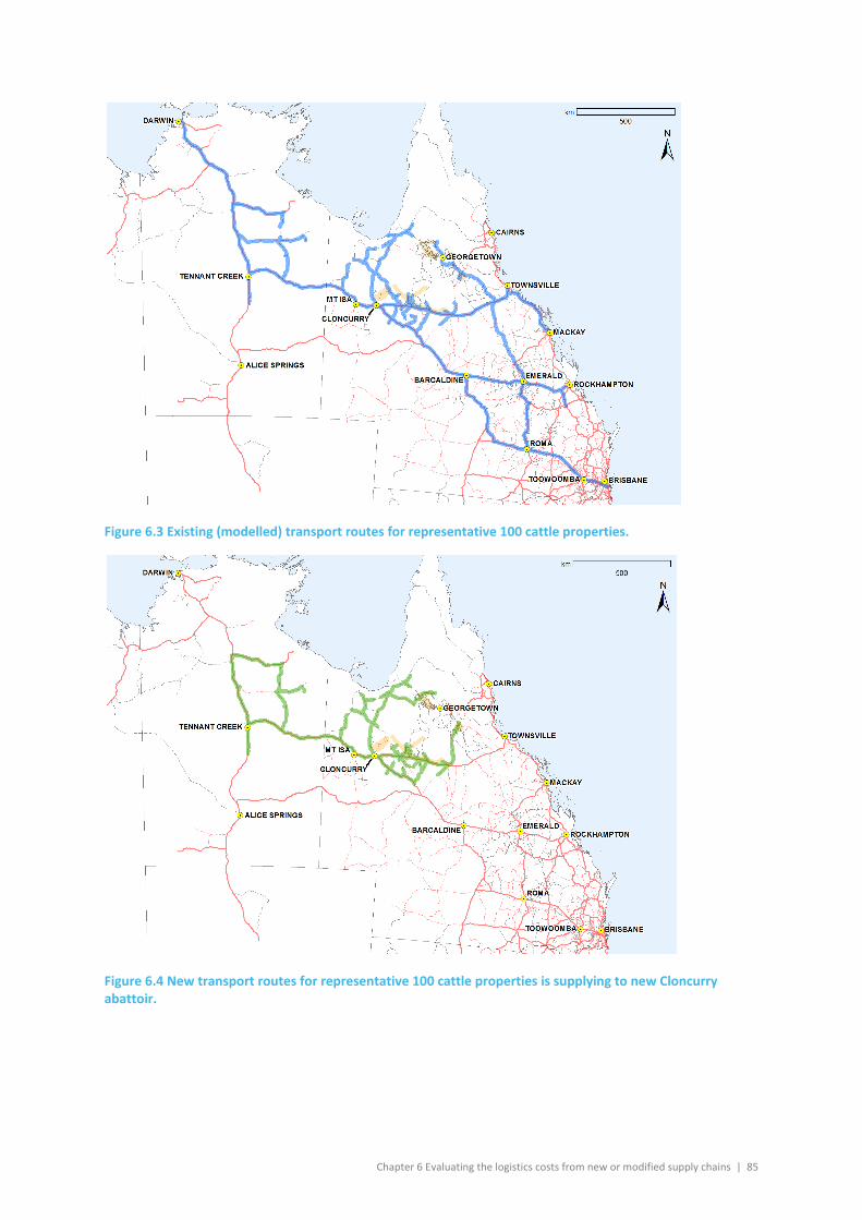
Chapter 6 Evaluating the logistics costs from new or modified supply chains | 85
Figure 6.3 Existing (modelled) transport routes for representative 100 cattle properties.
Figure 6.4 New transport routes for representative 100 cattle properties is supplying to new Cloncurry abattoir.
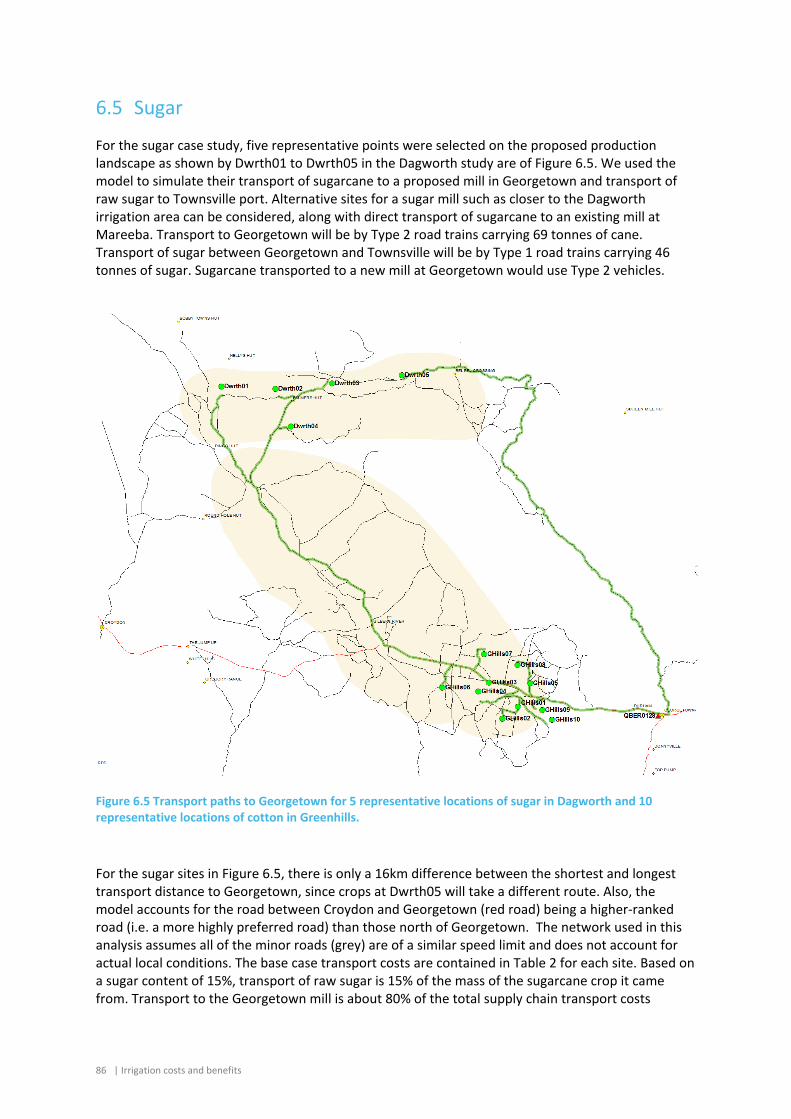
86 | Irrigation costs and benefits
6.5 Sugar
For the sugar case study, five representative points were selected on the proposed production landscape as shown by Dwrth01 to Dwrth05 in the Dagworth study are of Figure 6.5. We used the model to simulate their transport of sugarcane to a proposed mill in Georgetown and transport of raw sugar to Townsville port. Alternative sites for a sugar mill such as closer to the Dagworth irrigation area can be considered, along with direct transport of sugarcane to an existing mill at Mareeba. Transport to Georgetown will be by Type 2 road trains carrying 69 tonnes of cane. Transport of sugar between Georgetown and Townsville will be by Type 1 road trains carrying 46 tonnes of sugar. Sugarcane transported to a new mill at Georgetown would use Type 2 vehicles.
Figure 6.5 Transport paths to Georgetown for 5 representative locations of sugar in Dagworth and 10 representative locations of cotton in Greenhills.
For the sugar sites in Figure 6.5, there is only a 16km difference between the shortest and longest transport distance to Georgetown, since crops at Dwrth05 will take a different route. Also, the model accounts for the road between Croydon and Georgetown (red road) being a higher-ranked road (i.e. a more highly preferred road) than those north of Georgetown. The network used in this analysis assumes all of the minor roads (grey) are of a similar speed limit and does not account for actual local conditions. The base case transport costs are contained in Table 2 for each site. Based on a sugar content of 15%, transport of raw sugar is 15% of the mass of the sugarcane crop it came from. Transport to the Georgetown mill is about 80% of the total supply chain transport costs
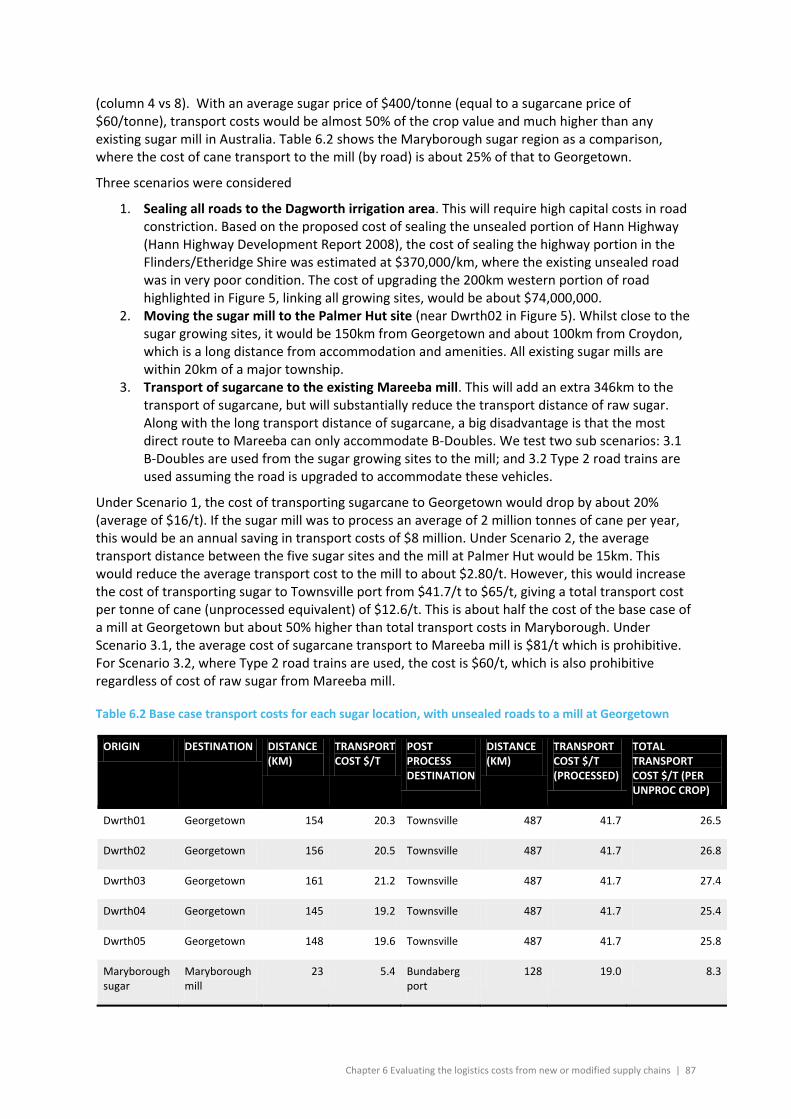
Chapter 6 Evaluating the logistics costs from new or modified supply chains | 87
(column 4 vs 8). With an average sugar price of $400/tonne (equal to a sugarcane price of $60/tonne), transport costs would be almost 50% of the crop value and much higher than any existing sugar mill in Australia. Table 6.2 shows the Maryborough sugar region as a comparison, where the cost of cane transport to the mill (by road) is about 25% of that to Georgetown.
Three scenarios were considered
1. Sealing all roads to the Dagworth irrigation area. This will require high capital costs in road constriction. Based on the proposed cost of sealing the unsealed portion of Hann Highway (Hann Highway Development Report 2008), the cost of sealing the highway portion in the Flinders/Etheridge Shire was estimated at $370,000/km, where the existing unsealed road was in very poor condition. The cost of upgrading the 200km western portion of road highlighted in Figure 5, linking all growing sites, would be about $74,000,000.
2. Moving the sugar mill to the Palmer Hut site (near Dwrth02 in Figure 5). Whilst close to the sugar growing sites, it would be 150km from Georgetown and about 100km from Croydon, which is a long distance from accommodation and amenities. All existing sugar mills are within 20km of a major township.
3. Transport of sugarcane to the existing Mareeba mill. This will add an extra 346km to the transport of sugarcane, but will substantially reduce the transport distance of raw sugar. Along with the long transport distance of sugarcane, a big disadvantage is that the most direct route to Mareeba can only accommodate B-Doubles. We test two sub scenarios: 3.1 B-Doubles are used from the sugar growing sites to the mill; and 3.2 Type 2 road trains are used assuming the road is upgraded to accommodate these vehicles.
Under Scenario 1, the cost of transporting sugarcane to Georgetown would drop by about 20% (average of $16/t). If the sugar mill was to process an average of 2 million tonnes of cane per year, this would be an annual saving in transport costs of $8 million. Under Scenario 2, the average transport distance between the five sugar sites and the mill at Palmer Hut would be 15km. This would reduce the average transport cost to the mill to about $2.80/t. However, this would increase the cost of transporting sugar to Townsville port from $41.7/t to $65/t, giving a total transport cost per tonne of cane (unprocessed equivalent) of $12.6/t. This is about half the cost of the base case of a mill at Georgetown but about 50% higher than total transport costs in Maryborough. Under Scenario 3.1, the average cost of sugarcane transport to Mareeba mill is $81/t which is prohibitive. For Scenario 3.2, where Type 2 road trains are used, the cost is $60/t, which is also prohibitive regardless of cost of raw sugar from Mareeba mill.
Table 6.2 Base case transport costs for each sugar location, with unsealed roads to a mill at Georgetown
ORIGIN DESTINATION DISTANCE (KM)
TRANSPORT COST $/T
POST PROCESS DESTINATION
DISTANCE (KM)
TRANSPORT COST $/T (PROCESSED)
TOTAL TRANSPORT COST $/T (PER UNPROC CROP)
Dwrth01 Georgetown 154 20.3 Townsville 487 41.7 26.5
Dwrth02 Georgetown 156 20.5 Townsville 487 41.7 26.8
Dwrth03 Georgetown 161 21.2 Townsville 487 41.7 27.4
Dwrth04 Georgetown 145 19.2 Townsville 487 41.7 25.4
Dwrth05 Georgetown 148 19.6 Townsville 487 41.7 25.8
Maryborough sugar
Maryborough mill
23 5.4 Bundaberg port
128 19.0 8.3
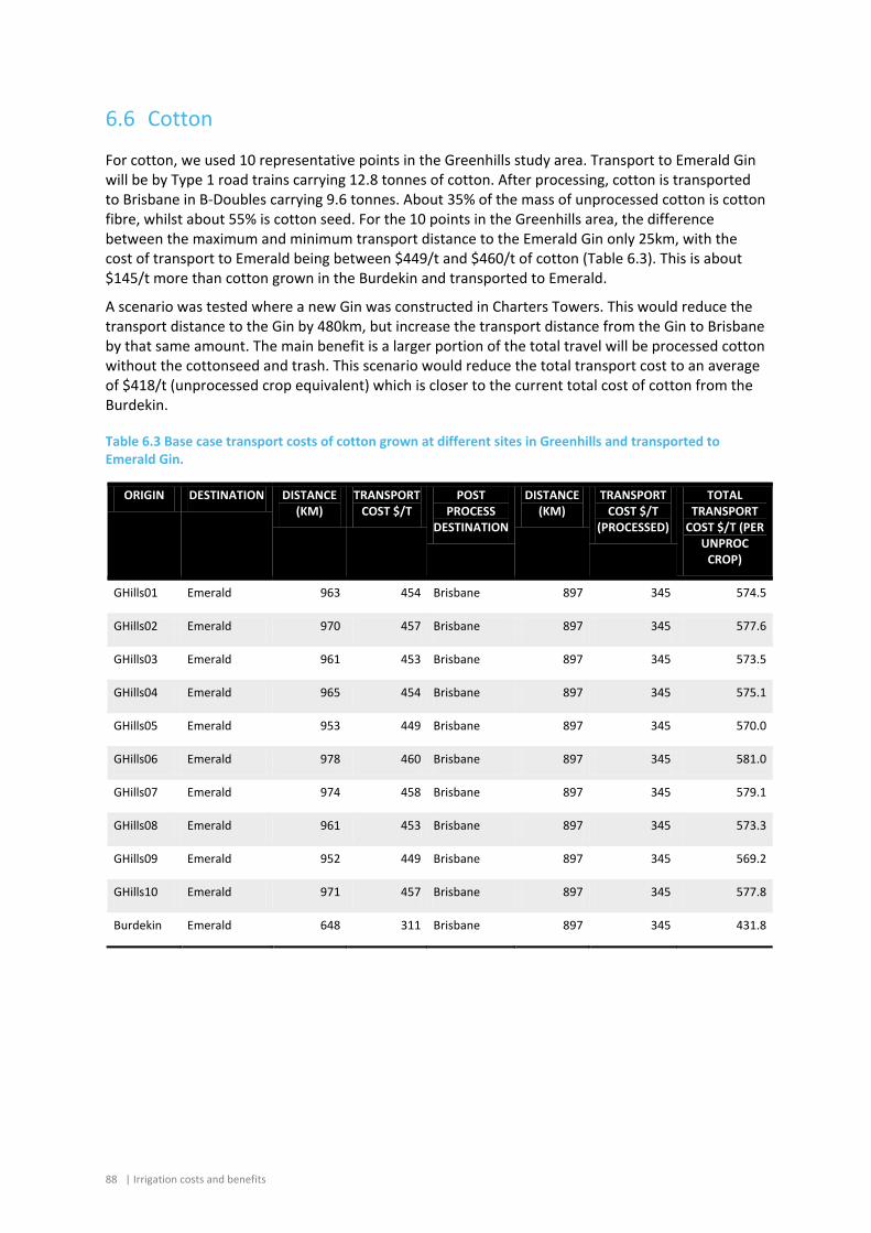
88 | Irrigation costs and benefits
6.6 Cotton
For cotton, we used 10 representative points in the Greenhills study area. Transport to Emerald Gin will be by Type 1 road trains carrying 12.8 tonnes of cotton. After processing, cotton is transported to Brisbane in B-Doubles carrying 9.6 tonnes. About 35% of the mass of unprocessed cotton is cotton fibre, whilst about 55% is cotton seed. For the 10 points in the Greenhills area, the difference between the maximum and minimum transport distance to the Emerald Gin only 25km, with the cost of transport to Emerald being between $449/t and $460/t of cotton (Table 6.3). This is about $145/t more than cotton grown in the Burdekin and transported to Emerald.
A scenario was tested where a new Gin was constructed in Charters Towers. This would reduce the transport distance to the Gin by 480km, but increase the transport distance from the Gin to Brisbane by that same amount. The main benefit is a larger portion of the total travel will be processed cotton without the cottonseed and trash. This scenario would reduce the total transport cost to an average of $418/t (unprocessed crop equivalent) which is closer to the current total cost of cotton from the Burdekin.
Table 6.3 Base case transport costs of cotton grown at different sites in Greenhills and transported to Emerald Gin.
ORIGIN DESTINATION DISTANCE (KM)
TRANSPORT COST $/T
POST PROCESS
DESTINATION
DISTANCE (KM)
TRANSPORT COST $/T
(PROCESSED)
TOTAL TRANSPORT
COST $/T (PER UNPROC
CROP)
GHills01 Emerald 963 454 Brisbane 897 345 574.5
GHills02 Emerald 970 457 Brisbane 897 345 577.6
GHills03 Emerald 961 453 Brisbane 897 345 573.5
GHills04 Emerald 965 454 Brisbane 897 345 575.1
GHills05 Emerald 953 449 Brisbane 897 345 570.0
GHills06 Emerald 978 460 Brisbane 897 345 581.0
GHills07 Emerald 974 458 Brisbane 897 345 579.1
GHills08 Emerald 961 453 Brisbane 897 345 573.3
GHills09 Emerald 952 449 Brisbane 897 345 569.2
GHills10 Emerald 971 457 Brisbane 897 345 577.8
Burdekin Emerald 648 311 Brisbane 897 345 431.8
Chapter 7 Conclusion | 89
7 Conclusion
The analyses reported here examined various dimensions of the costs and benefits associated with irrigation development at a range of scales, from on-farm and scheme-scale costs and benefits, through to regional and national impacts. Although this report can be read as a stand-alone document, its primary purpose is to provide the detail behind the analyses presented in the Flinders and Gilbert Agricultural Resource Assessment Catchment Reports (Petheram et al., 2013 a,b). It is recommended that readers of this report also read the Catchment Reports for more contextual material. Key findings presented in the report are:
• An analysis of incorporating irrigated forages into representative beef operations in the Flinders and Gilbert catchments suggest that the increased revenues from cattle production are not sufficient to offset the costs which include capital costs of on-farm dams and irrigation infrastructure.
• An analysis of the net benefits of investing in irrigation to undertake cropping also shows that capital costs of irrigation development impact substantially on investment performance, and that crop gross margins may need to be sustained reliably and at high levels to offset costs. There are, however, profitable opportunities.
• A generic scheme-scale analysis explored the whole-of-development financial performance under a range of scheme-scale capital costs and sizes of irrigation developments. Irrigators could not afford to pay a price to fully cover scheme capital and operating costs, expect under a limited set of circumstances (of low capital costs and high gross margins).
• A large set of Acts of legislation are applicable to irrigation development – the implication for irrigation development should be assessed on a case by case basis.
• A regional-scale analysis of implementing several irrigation developments and associated processing facilities in the Flinders and Gilbert catchments shows the potential for the enlargement of the regional economy of North-West Queensland, but a negative economic impact for the nation.
• Building a new abattoir in Cloncurry and a new cotton gin in Carters Towers can result in substantial transport cost savings to Flinders beef producers and cotton growers. Sugarcane growers in the Gilbert (serviced by a dam in Dagworth) could benefit from reduced transport costs from a sugar mill in Palmers Hut, but the trade-off is the 100+km distance from Georgetown.
90 | Irrigation costs and benefits
8 References
ABARES (2013a) Agricultural commodities: June quarter 2013, Australian Bureau of Agricultural and Resource Economics and Sciences, Canberra.
ABARES (2013b) Australian crop report, Australian Bureau of Agricultural and Resource Economics and Sciences, Canberra, June.
Barber, M. (2013) Indigenous water values for the Flinders catchment. A technical report to the Australian Government from the CSIRO Flinders and Gilbert Agricultural Resource Assessment, part of the North Queensland Irrigated Agriculture Strategy. CSIRO Water for a Healthy Country and Sustainable Agriculture flagships, Australia.
Bartley R., Thomas M., Clifford D., Philip S., Brough D., Harms B., Willis R., Gregory L., Glover M., Moodie K., Sugars M., Eyre L., Smith D., Hicks W. & Petheram C. (2013). Land suitability: technical methods. A technical report to the Australian Government from the CSIRO Flinders and Gilbert Agricultural Resource Assessment, part of the North Queensland Irrigated Agriculture Strategy. In. CSIRO Water for a Healthy Country and Sustainable Agriculture flagships Australia
CSIRO, JCU and TCI (2013) Land tenure in northern Australia: opportunities and challenges for investment. Prepared for the North Australian Ministerial Forum by CSIRO, James Cook University and the Cairns Institute, Townsville, Queensland. Viewed 15 August 2013. <http://www.regional.gov.au/regional/ona/land-tenure/pdfs/land-tenure-20130717.pdf>.
Culpitt, R (2011) Healthy HeadWaters. Farm level economic and financial modelling of alternative irrigation practices. Synergies Economic Consulting, Brisbane, Queensland.
DERM (2010a) Regulation of referable dams. Department of Environment and Resource Management, Queensland. Viewed 10 October 2013, <www.agforceqld.org.au/file.php?id=844&open=yes>.
DERM (2010b) A guide to land tenure under the Land Act 1994. Department of Environment and Resource Management, Queensland.
DERM (2011a) Guidelines for negotiating an Indigenous land use agreement (area agreement). Department of Environmental and Resource Management. Queensland Government, Brisbane.
DERM (2011b) Guide to the pastoral ILUA template. Department of Environmental and Resource Management. Queensland Government, Brisbane
DNRM (2012) Water Resources (Gulf) Plan 2007: sale of unallocated water, tender documents. Department of Natural Resources, Mines and Energy, Queensland. Viewed 10 October 2013, <http://www.nrm.qld.gov.au/wrp/pdf/unallocated_water/gulf-uaw-tender.pdf>.
DNRME (2004) Agricultural land and water resource assessment report supporting Gulf and Mitchell water resource planning. Report No. 18492. Department of Natural Resources, Mines and Energy, Brisbane
EDO (2012) Factsheet: an introduction to the Sustainable Planning Act 2009 (Qld). Environmental Defenders Office, Brisbane. Viewed 28 November 2013, <www.edo.org.au/edoqld/wp-content/uploads/2012/05/11.02-Factsheet1.pdf>.
FAO (2013) Food Outlook November 2013. Special Features report. Accessed 2/12/13 at http://www.fao.org/fileadmin/templates/worldfood/Reports_and_docs/Special_feature_FFPI_en.pdf
Chapter 8 References | 91
Gleeson T, Martin P, Mifsud C (2012) Northern Australian beef industry: Assessment of risks and opportunities. ABARES report to client prepared for the Northern Australia Ministerial Forum, Canberra, May. Canberra.
Gramshaw, D. and Lloyd, P. (1993). Grazing the north. Creating wealth and sustaining the land. Queensland Department of Primary Industries, Information Series, QI92042., Brisbane.
Gulf Regional Planning Advisory Committee. (2000). Gulf Regional Development Plan. Cairns: State of Queensland.
Hann Highway Development Report (2008). Economic Impact Benefit Cost Analysis. Prepared by WS Cummings for Hann Highway Action Group.
Harrison, W. J., & Pearson, K. R. (1996). Computing Solutions for Large General Equilibrium Models Using GEMPACK. Computational Economics, 9, 83-127.
Higgins A, Watson I, Chilcott C, Zhou M, Garcia-Flores R, Eady S, McFallan S, Prestwidge D, Laredo L. (2013). Optimising Capital Investment and Operations for the Livestock Industry in Northern Australia. The Rangeland Journal, 35, 181-191.
Horridge, M., Madden, J., & Wittwer, G. (2005). The impact of the 2002–2003 drought on Australia. Journal of Policy Modeling, 27(3), 285-308.
Keating BA, Carberry PC, Hammer GL, Probert ME, Robertson MJ, Holzworth D, Huth NI, Hargreaves JNG, Meinke H, Hochman Z, McLean G, Verburg K, Snow V, Dimes JP, Silburn M, Wang E, Brown S, Bristow KL, Asseng S, Chapman S, McCown RL, Freebairn DM, Smith CJ (2003) An overview of APSIM, a model designed for farming systems simulation. European Journal of Agronomy 18, 267–288
Littleboy M, McKeon GM (1997) Subroutine GRASP: Grass Production Model. Documentation of the Marcoola Version of Subroutine GRASP. Appendix 2 of “Evaluating the risks of pasture and land degradation in native pasture in Queensland”. Final Project Report for the Rural Industries Research and Development Corporation DAQ124A, pp. 76
Mason (2009) Gilbert River agricultural precinct proposal. Scoping brief on the proposed Gilbert River agricultural precinct, including a marketing and gross margin analysis perspective. The State of Queensland, Department of Employment, Economic Development and Innovation.
Mason, G. and Larard, A (2011) A case study analysis of cropping and grazing systems for Flinders River Agricultural Precinct Development Project. The State of Queensland, Department of Employment, Economic Development and Innovation.
McCosker T, McLean D, Holmes P (2009) Northern beef situation analysis 2009 – Final report for the Meat & Livestock Australia (MLA), August 2010
McDonald C (2012) IAT_na – Integrated Analysis Tool for North Australian Beef Properties, Users Guide - Version P1.07, June 2012, CSIRO Ecosystem Sciences
McGrath C (2011) Synopsis of the Queensland environmental legal system, 5th edition. Environmental Law Publishing, Brisbane.
McFallan S, Higgins A, Prestwidge D, Laredo L. (2013). A GIS model for simulating infrastructure investments in livestock logistics: Application to the northern beef industry. Proceedings of MODSIM 2013, In press.
Meat and Livestock Australia (2013) MLA data: Farm survey data for the beef, slaughter lambs and sheep industries. Viewed 08 October 2013 <http://apps.daff.gov.au/MLA/mla.asp>.
National Water Commission (2009) Australian Water Reform 2009: Second biennial assessment of progress in implementation of the National Water Initiative, September 2009, Canberra.
92 | Irrigation costs and benefits
New South Wales Department of Primary Industries (2013) Farm Budgets and Costs. Availble at: http://www.dpi.nsw.gov.au/agriculture/farm-business/budgets. Last accessed 2/12/13.
Pannell D (1997) Sensitivity analysis of normative economic models: theoretical framework and practical strategies. Agricultural Economics, 16, 139–152
Petheram C, Watson I and Stone P (eds) (2013a) Agricultural resource assessment for the Flinders catchment. A report to the Australian Government from the CSIRO Flinders and Gilbert Agricultural Resource Assessment, part of the North Queensland Irrigated Agriculture Strategy. CSIRO Water for a Healthy Country and Sustainable Agriculture flagships, Australia.
Petheram C, Watson I and Stone P (eds) (2013b) Agricultural resource assessment for the Gilbert catchment. A report to the Australian Government from the CSIRO Flinders and Gilbert Agricultural Resource Assessment, part of the North Queensland Irrigated Agriculture Strategy. CSIRO Water for a Healthy Country and Sustainable Agriculture flagships, Australia.
Petheram C, Yang A (2013) Climatic data and their characterisation for hydrological and agricultural scenario modelling across the Flinders and Gilbert catchments. A technical report to the Australian Government from the CSIRO Flinders and Gilbert Agricultural Resource Assessment, part of the North Queensland Irrigated Agriculture Strategy. CSIRO Water for a Healthy Country and Sustainable Agriculture flagships, Australia
Queensland Government (2010). Agbiz: Queensland agribusiness decision toolkit. Available at: http://agbiz.daff.qld.gov.au/plants/field-crops-pastures.htm. Last accessed 2/12/13.
Queensland Government (2000) Guidelines for Financial and Economic Evaluation of New Water Infrastructure in Queensland. Queensland Government Treasury, Brisbane.
Queensland Government. (2010). North West Regional Plan 2010-2031 Planning for a stronger, more liveable and sustainable community. City East: Queensland Government.
Queensland Law Society (2008) Legal guide for primary producers. Queensland Law Society, Brisbane.
Schatz, T. (2012) Heifer management in northern beef herds. Meat and Livestock Australia, North Sydney
SDIIC (2012) Interim report: inquiry into the future and continued relevance of government land tenure across Queensland. Report No. 17. State Development, Infrastructure and Industry Committee, Queensland.
Stutz K (2012) Assessment of the institutional complexity associated with agricultural development.Industrial Placement Report, University of Queensland and CSIRO, Brisbane.
Webster, T., Morison, J., Abel, N., Clark, E., Rippin, L., Herr, A., . . . Stone, P. (2009). Irrigated Agriculture: Development Opportunities and Implications for Northern Australia. In P. Stone (Ed.), Northern Australia Land and Water Science Review. Canberra: CSIRO.
Webster T and Poulton P (2013) Agricultural production in the Flinders and Gilbert catchments. A technical report to the Australian Government from the CSIRO Flinders and Gilbert Agricultural Resource Assessment, part of the North Queensland Irrigated Agriculture Strategy. CSIRO Water for a Healthy Country and Sustainable Agriculture flagships, Australia
Wittwer G (ed) (2012) Economic modeling of water: the Australian CGE Experience (Vol. 3). Springer, Dordrecht, Netherlands.
Wittwer, G., Vere, D. T., Jones, R. E., & Griffith, G. R. (2005). Dynamic general equilibrium analysis of improved weed management in Australia's winter cropping systems. Australian Journal of Agricultural and Resource Economics, 49(4), 363-377. doi: 10.1111/j.1467-8489.2005.00308.x
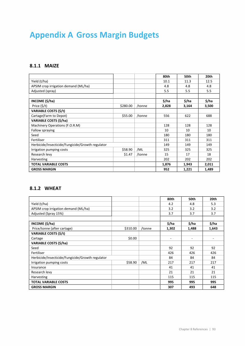
Chapter 8 References | 93
Appendix A Gross Margin Budgets
8.1.1 MAIZE
80th 50th 20th Yield (t/ha) 10.1 11.3 12.5 APSIM crop irrigation demand (ML/ha) 4.8 4.8 4.8 Adjusted (spray) 5.5 5.5 5.5
INCOME ($/ha) $/ha $/ha $/ha Price ($/t) $280.00 /tonne 2,828 3,164 3,500 VARIABLE COSTS ($/t) Cartage(Farm to Depot) $55.00 /tonne 556 622 688 VARIABLE COSTS ($/ha) Machinery Operations (F.O.R.M) 128 128 128 Fallow spraying 10 10 10 Seed 180 180 180 Fertiliser 311 311 311 Herbicide/Insecticide/Fungicide/Growth regulator 149 149 149 Irrigation pumping costs $58.90 /ML 325 325 325 Research levy $1.47 /tonne 15 17 18 Harvesting 202 202 202 TOTAL VARIABLE COSTS 1,876 1,943 2,011 GROSS MARGIN 952 1,221 1,489
8.1.2 WHEAT
80th 50th 20th Yield (t/ha) 4.2 4.8 5.3 APSIM crop irrigation demand (ML/ha) 3.2 3.2 3.2 Adjusted (Spray 15%) 3.7 3.7 3.7
INCOME ($/ha) $/ha $/ha $/ha Price/tonne (after cartage) $310.00 /tonne 1,302 1,488 1,643 VARIABLE COSTS ($/t) Cartage $0.00 - - - VARIABLE COSTS ($/ha) Seed 92 92 92 Fertiliser 426 426 426 Herbicide/Insecticide/Fungicide/Growth regulator 84 84 84 Irrigation pumping costs $58.90 /ML 217 217 217 Insurance 41 41 41 Research levy 21 21 21 Harvesting 115 115 115 TOTAL VARIABLE COSTS 995 995 995 GROSS MARGIN 307 493 648
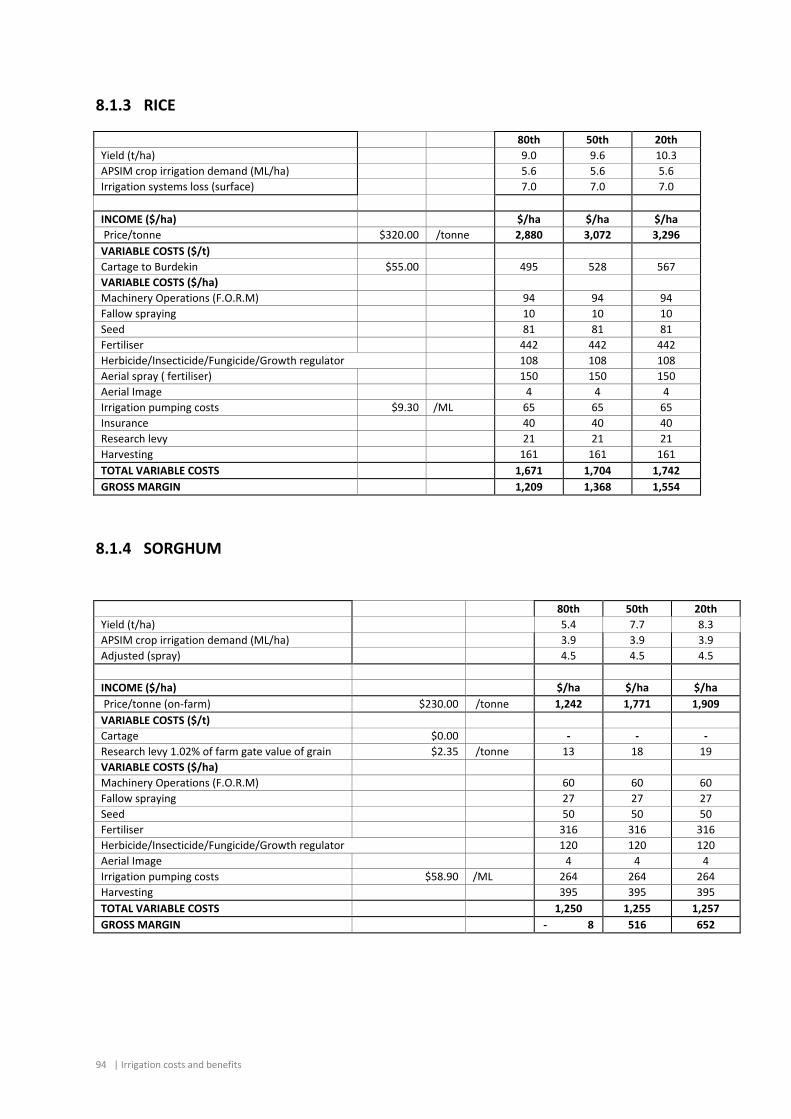
94 | Irrigation costs and benefits
8.1.3 RICE
80th 50th 20th Yield (t/ha) 9.0 9.6 10.3 APSIM crop irrigation demand (ML/ha) 5.6 5.6 5.6 Irrigation systems loss (surface) 7.0 7.0 7.0
INCOME ($/ha) $/ha $/ha $/ha Price/tonne $320.00 /tonne 2,880 3,072 3,296 VARIABLE COSTS ($/t) Cartage to Burdekin $55.00 495 528 567 VARIABLE COSTS ($/ha) Machinery Operations (F.O.R.M) 94 94 94 Fallow spraying 10 10 10 Seed 81 81 81 Fertiliser 442 442 442 Herbicide/Insecticide/Fungicide/Growth regulator 108 108 108 Aerial spray ( fertiliser) 150 150 150 Aerial Image 4 4 4 Irrigation pumping costs $9.30 /ML 65 65 65 Insurance 40 40 40 Research levy 21 21 21 Harvesting 161 161 161 TOTAL VARIABLE COSTS 1,671 1,704 1,742 GROSS MARGIN 1,209 1,368 1,554
8.1.4 SORGHUM
80th 50th 20th Yield (t/ha) 5.4 7.7 8.3 APSIM crop irrigation demand (ML/ha) 3.9 3.9 3.9 Adjusted (spray) 4.5 4.5 4.5 INCOME ($/ha) $/ha $/ha $/ha Price/tonne (on-farm) $230.00 /tonne 1,242 1,771 1,909 VARIABLE COSTS ($/t) Cartage $0.00 - - - Research levy 1.02% of farm gate value of grain $2.35 /tonne 13 18 19 VARIABLE COSTS ($/ha) Machinery Operations (F.O.R.M) 60 60 60 Fallow spraying 27 27 27 Seed 50 50 50 Fertiliser 316 316 316 Herbicide/Insecticide/Fungicide/Growth regulator 120 120 120 Aerial Image 4 4 4 Irrigation pumping costs $58.90 /ML 264 264 264 Harvesting 395 395 395 TOTAL VARIABLE COSTS 1,250 1,255 1,257 GROSS MARGIN - 8 516 652
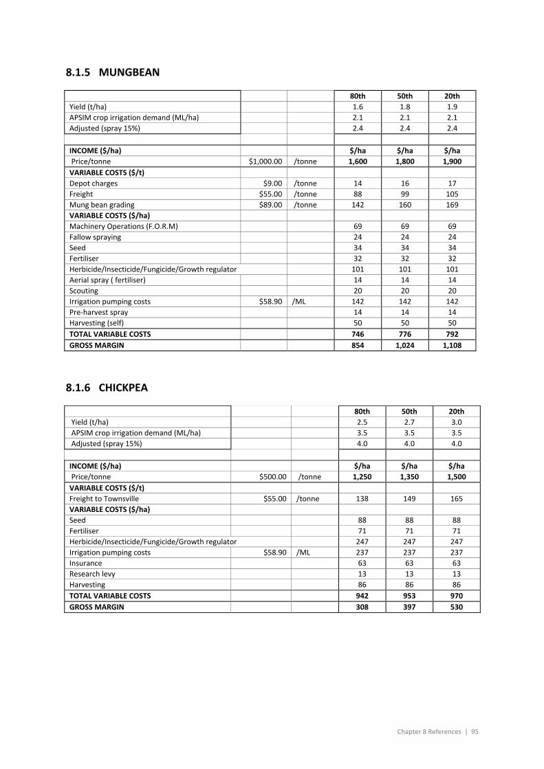
Chapter 8 References | 95
8.1.5 MUNGBEAN
80th 50th 20th Yield (t/ha) 1.6 1.8 1.9 APSIM crop irrigation demand (ML/ha) 2.1 2.1 2.1 Adjusted (spray 15%) 2.4 2.4 2.4
INCOME ($/ha) $/ha $/ha $/ha Price/tonne $1,000.00 /tonne 1,600 1,800 1,900 VARIABLE COSTS ($/t) Depot charges $9.00 /tonne 14 16 17 Freight $55.00 /tonne 88 99 105 Mung bean grading $89.00 /tonne 142 160 169 VARIABLE COSTS ($/ha) Machinery Operations (F.O.R.M) 69 69 69 Fallow spraying 24 24 24 Seed 34 34 34 Fertiliser 32 32 32 Herbicide/Insecticide/Fungicide/Growth regulator 101 101 101 Aerial spray ( fertiliser) 14 14 14 Scouting 20 20 20 Irrigation pumping costs $58.90 /ML 142 142 142 Pre-harvest spray 14 14 14 Harvesting (self) 50 50 50 TOTAL VARIABLE COSTS 746 776 792 GROSS MARGIN 854 1,024 1,108
8.1.6 CHICKPEA
80th 50th 20th Yield (t/ha) 2.5 2.7 3.0 APSIM crop irrigation demand (ML/ha) 3.5 3.5 3.5 Adjusted (spray 15%) 4.0 4.0 4.0
INCOME ($/ha) $/ha $/ha $/ha Price/tonne $500.00 /tonne 1,250 1,350 1,500 VARIABLE COSTS ($/t) Freight to Townsville $55.00 /tonne 138 149 165 VARIABLE COSTS ($/ha) Seed 88 88 88 Fertiliser 71 71 71 Herbicide/Insecticide/Fungicide/Growth regulator 247 247 247 Irrigation pumping costs $58.90 /ML 237 237 237 Insurance 63 63 63 Research levy 13 13 13 Harvesting 86 86 86 TOTAL VARIABLE COSTS 942 953 970 GROSS MARGIN 308 397 530
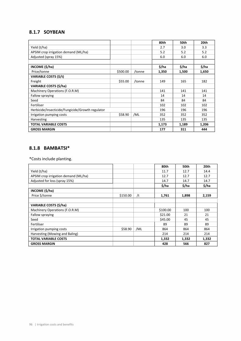
96 | Irrigation costs and benefits
8.1.7 SOYBEAN
80th 50th 20th Yield (t/ha) 2.7 3.0 3.3 APSIM crop irrigation demand (ML/ha) 5.2 5.2 5.2 Adjusted (spray 15%) 6.0 6.0 6.0
INCOME ($/ha) $/ha $/ha $/ha Price/tonne $500.00 /tonne 1,350 1,500 1,650 VARIABLE COSTS ($/t) Freight $55.00 /tonne 149 165 182 VARIABLE COSTS ($/ha) Machinery Operations (F.O.R.M) 141 141 141 Fallow spraying 14 14 14 Seed 84 84 84 Fertiliser 102 102 102 Herbicide/Insecticide/Fungicide/Growth regulator 196 196 196 Irrigation pumping costs $58.90 /ML 352 352 352 Harvesting 135 135 135 TOTAL VARIABLE COSTS 1,173 1,189 1,206 GROSS MARGIN 177 311 444
8.1.8 BAMBATSI*
*Costs include planting.
80th 50th 20th Yield (t/ha) 11.7 12.7 14.4 APSIM crop irrigation demand (ML/ha) 12.7 12.7 12.7 Adjusted for loss (spray 15%) 14.7 14.7 14.7
$/ha $/ha $/ha INCOME ($/ha) Price $/tonne $150.00 /t 1,761 1,898 2,159 VARIABLE COSTS ($/ha) Machinery Operations (F.O.R.M) $100.00 100 100 Fallow spraying $21.00 21 21 Seed $45.00 45 45 Fertiliser 89 89 89 Irrigation pumping costs $58.90 /ML 864 864 864 Harvesting (Mowing and Baling) 214 214 214 TOTAL VARIABLE COSTS 1,332 1,332 1,332 GROSS MARGIN 428 566 827
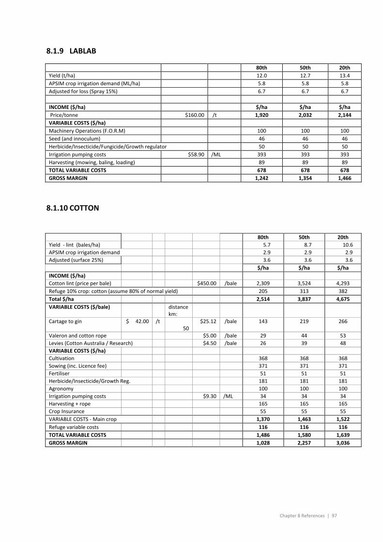
Chapter 8 References | 97
8.1.9 LABLAB
80th 50th 20th Yield (t/ha) 12.0 12.7 13.4 APSIM crop irrigation demand (ML/ha) 5.8 5.8 5.8 Adjusted for loss (Spray 15%) 6.7 6.7 6.7
INCOME ($/ha) $/ha $/ha $/ha Price/tonne $160.00 /t 1,920 2,032 2,144 VARIABLE COSTS ($/ha) Machinery Operations (F.O.R.M) 100 100 100 Seed (and innoculum) 46 46 46 Herbicide/Insecticide/Fungicide/Growth regulator 50 50 50 Irrigation pumping costs $58.90 /ML 393 393 393 Harvesting (mowing, baling, loading) 89 89 89 TOTAL VARIABLE COSTS 678 678 678 GROSS MARGIN 1,242 1,354 1,466
8.1.10 COTTON
80th 50th 20th Yield - lint (bales/ha) 5.7 8.7 10.6 APSIM crop irrigation demand 2.9 2.9 2.9 Adjusted (surface 25%) 3.6 3.6 3.6
$/ha $/ha $/ha INCOME ($/ha) Cotton lint (price per bale) $450.00 /bale 2,309 3,524 4,293 Refuge 10% crop: cotton (assume 80% of normal yield) 205 313 382 Total $/ha 2,514 3,837 4,675 VARIABLE COSTS ($/bale) distance
km:
Cartage to gin $ 42.00 /t 50
$25.12 /bale 143 219 266
Valeron and cotton rope $5.00 /bale 29 44 53 Levies (Cotton Australia / Research) $4.50 /bale 26 39 48 VARIABLE COSTS ($/ha) Cultivation 368 368 368 Sowing (inc. Licence fee) 371 371 371 Fertiliser 51 51 51 Herbicide/Insecticide/Growth Reg. 181 181 181 Agronomy 100 100 100 Irrigation pumping costs $9.30 /ML 34 34 34 Harvesting + rope 165 165 165 Crop Insurance 55 55 55 VARIABLE COSTS - Main crop 1,370 1,463 1,522 Refuge variable costs 116 116 116 TOTAL VARIABLE COSTS 1,486 1,580 1,639 GROSS MARGIN 1,028 2,257 3,036
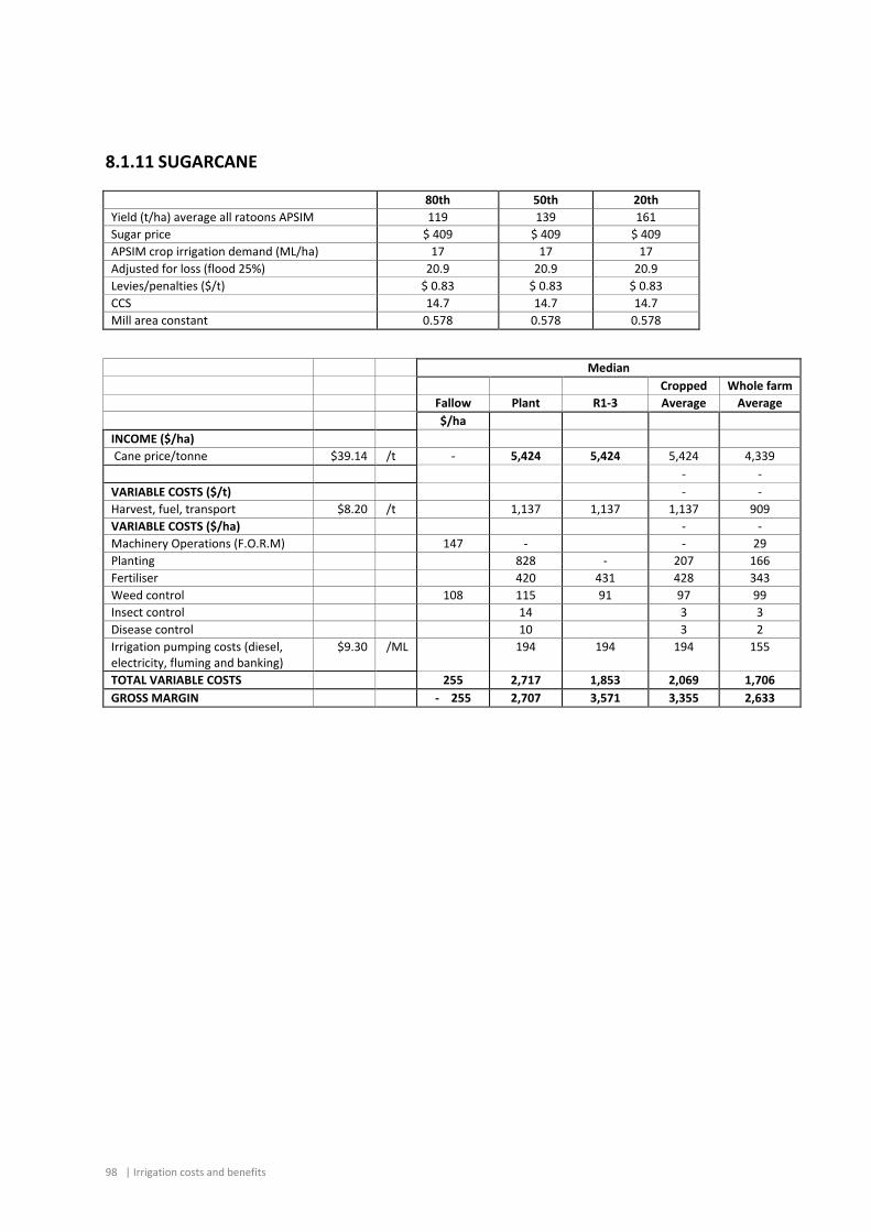
98 | Irrigation costs and benefits
8.1.11 SUGARCANE
80th 50th 20th Yield (t/ha) average all ratoons APSIM 119 139 161 Sugar price $ 409 $ 409 $ 409 APSIM crop irrigation demand (ML/ha) 17 17 17 Adjusted for loss (flood 25%) 20.9 20.9 20.9 Levies/penalties ($/t) $ 0.83 $ 0.83 $ 0.83 CCS 14.7 14.7 14.7 Mill area constant 0.578 0.578 0.578
Median Cropped Whole farm Fallow Plant R1-3 Average Average
$/ha INCOME ($/ha) Cane price/tonne $39.14 /t - 5,424 5,424 5,424 4,339 - - VARIABLE COSTS ($/t) - - Harvest, fuel, transport $8.20 /t 1,137 1,137 1,137 909 VARIABLE COSTS ($/ha) - - Machinery Operations (F.O.R.M) 147 - - 29 Planting 828 - 207 166 Fertiliser 420 431 428 343 Weed control 108 115 91 97 99 Insect control 14 3 3 Disease control 10 3 2 Irrigation pumping costs (diesel, electricity, fluming and banking)
$9.30 /ML 194 194 194 155
TOTAL VARIABLE COSTS 255 2,717 1,853 2,069 1,706 GROSS MARGIN - 255 2,707 3,571 3,355 2,633
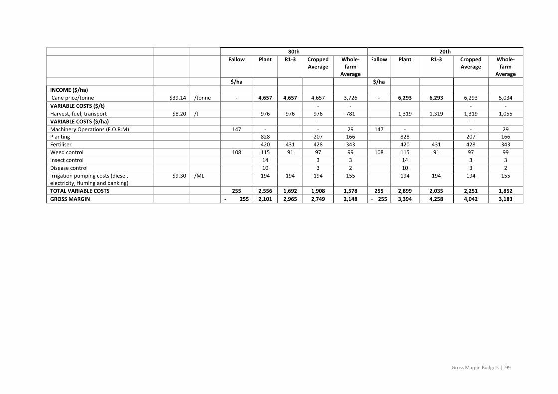
Gross Margin Budgets | 99
80th 20th Fallow Plant R1-3 Cropped
Average Whole-
farm Average
Fallow Plant R1-3 Cropped Average
Whole-farm
Average $/ha $/ha
INCOME ($/ha) Cane price/tonne $39.14 /tonne - 4,657 4,657 4,657 3,726 - 6,293 6,293 6,293 5,034 VARIABLE COSTS ($/t) - - - - Harvest, fuel, transport $8.20 /t 976 976 976 781 1,319 1,319 1,319 1,055 VARIABLE COSTS ($/ha) - - - - Machinery Operations (F.O.R.M) 147 - - 29 147 - - 29 Planting 828 - 207 166 828 - 207 166 Fertiliser 420 431 428 343 420 431 428 343 Weed control 108 115 91 97 99 108 115 91 97 99 Insect control 14 3 3 14 3 3 Disease control 10 3 2 10 3 2 Irrigation pumping costs (diesel, electricity, fluming and banking)
$9.30 /ML 194 194 194 155 194 194 194 155
TOTAL VARIABLE COSTS 255 2,556 1,692 1,908 1,578 255 2,899 2,035 2,251 1,852 GROSS MARGIN - 255 2,101 2,965 2,749 2,148 - 255 3,394 4,258 4,042 3,183
100 | Irrigation costs and benefits
CONTACT US t 1300 363 400 +61 3 9545 2176 e [email protected] w www.csiro.au
YOUR CSIRO Australia is founding its future on science and innovation. Its national science agency, CSIRO, is a powerhouse of ideas, technologies and skills for building prosperity, growth, health and sustainability. It serves governments, industries, business and communities across the nation.
FOR FURTHER INFORMATION Water for a Healthy Country Flagship Lisa Brennan McKellar t +61 7 3833 5653 e [email protected] w csiro.au/Organisation-Structure/Flagships/ Water-for-a-Healthy-Country-Flagship.aspx