UNIVERSITY OF OSLODepartment of Informatics

Flexinol asActuator for aHumanoid Finger -Possibilities andChallenges

Master thesis (60 pt)

Øyvind FjellangSæther

01.11.2008

Abstract

Robots become more and more common in our every day lives as technology develops. Robots arenormally actuated by pneumatics, hydraulics or servo motors. These technologies are mature and widelyused, but other less commonly used actuators are also available. Among these we find the artificial musclefiber Flexinol which belongs to a class of materials known as Shape Memory Alloys.

This thesis aims to implement the artificial muscle fiber Flexinol as actuator for a humanoid finger.The first part of the thesis focuses on testing of single Flexinol wires to determine in what degree theseare suitable for long term use as actuators. A test frame is built to investigate contraction speed, forceand displacement for wires in different setups. Among these are tests with a small dead weight, a largedead weight, an antagonistic setup and a setup with a spring working as a passive antagonistic force.

The second part of the thesis makes use of Flexinol as actuator when designing and prototyping ahumanoid finger. The human finger is used as inspiration in this part, applying tendons and musclesin a human-like way. The finger is designed with CAD-software and then printed in plastic. It is thenassembled with tendons and actuated with three Flexinol wires. Finally, an attempt to control thehumanoid finger is done.

Specially designed software and hardware is developed through the thesis to implement workingexperiments. Software for both a laboratory computer and a microcontroller is written to control thesystem and to collect sensory data respectively.

I

II

Preface

This thesis is part of my Master Degree at the University of Oslo, Department of Informatics. The thesiswas carried out during 2008 in the research group Robotics and Intelligent Systems (ROBIN). First ofall I want to thank my supervisor, Associate Professor Mats Høvin, for creative input, for motivating meto be creative and for valuable feedback both during my practical work and during writing.

I also want to thank the following (sorted by topic): Vegard Friis Ruud, Charlotte Kristiansen, MarieKlemsdahl Eklund and Marte Lødemel Henriksen for fruitful discussions regarding the human anatomy,Kjetil Stiansen for help regarding practical and theoretical electronics and Andreas Gimmestad for hislinguistic abilities.

Thanks also go to friends and family for showing interest, specially to my father Dag Henning Sætherfor guidance both during my practical work and during writing.

Øyvind Fjellang SætherNovember 2008

III

IV

Contents

1 Introduction 11.1 Humanoid Hands . . . . . . . . . . . . . . . . . . . . . . . . . . . . . . . . . . . . . . . . . 11.2 Robot Hand Actuation . . . . . . . . . . . . . . . . . . . . . . . . . . . . . . . . . . . . . . 21.3 Flexinol - Artificial Muscle Fibers . . . . . . . . . . . . . . . . . . . . . . . . . . . . . . . . 31.4 Thesis Overview . . . . . . . . . . . . . . . . . . . . . . . . . . . . . . . . . . . . . . . . . 41.5 Short Conclusion . . . . . . . . . . . . . . . . . . . . . . . . . . . . . . . . . . . . . . . . . 5

2 Background 72.1 Anatomy of The Human Hand . . . . . . . . . . . . . . . . . . . . . . . . . . . . . . . . . 7

2.1.1 Skeleton . . . . . . . . . . . . . . . . . . . . . . . . . . . . . . . . . . . . . . . . . . 72.1.2 Tendons and Muscles . . . . . . . . . . . . . . . . . . . . . . . . . . . . . . . . . . 82.1.3 Robotic Approach to the Human Hand . . . . . . . . . . . . . . . . . . . . . . . . 8

2.2 Traditional Actuators . . . . . . . . . . . . . . . . . . . . . . . . . . . . . . . . . . . . . . 92.2.1 Hydraulics . . . . . . . . . . . . . . . . . . . . . . . . . . . . . . . . . . . . . . . . 92.2.2 Pneumatics . . . . . . . . . . . . . . . . . . . . . . . . . . . . . . . . . . . . . . . . 92.2.3 Servo Motors . . . . . . . . . . . . . . . . . . . . . . . . . . . . . . . . . . . . . . . 102.2.4 Stepper Motors . . . . . . . . . . . . . . . . . . . . . . . . . . . . . . . . . . . . . . 122.2.5 Electric Solenoids . . . . . . . . . . . . . . . . . . . . . . . . . . . . . . . . . . . . . 13

2.3 Intelligent Materials used as Actuators . . . . . . . . . . . . . . . . . . . . . . . . . . . . . 132.3.1 Shape Memory Alloys in General . . . . . . . . . . . . . . . . . . . . . . . . . . . . 132.3.2 Flexinol . . . . . . . . . . . . . . . . . . . . . . . . . . . . . . . . . . . . . . . . . . 152.3.3 Electroactive Polymers . . . . . . . . . . . . . . . . . . . . . . . . . . . . . . . . . . 22

2.4 Actuator Comparison . . . . . . . . . . . . . . . . . . . . . . . . . . . . . . . . . . . . . . 222.4.1 Power to Weight Ratio . . . . . . . . . . . . . . . . . . . . . . . . . . . . . . . . . . 23

2.5 Feedback Sensors . . . . . . . . . . . . . . . . . . . . . . . . . . . . . . . . . . . . . . . . . 232.5.1 Displacement Transducers . . . . . . . . . . . . . . . . . . . . . . . . . . . . . . . . 242.5.2 Force Transducers . . . . . . . . . . . . . . . . . . . . . . . . . . . . . . . . . . . . 25

3 Used Tools 293.1 Atmel AVR Microcontrollers . . . . . . . . . . . . . . . . . . . . . . . . . . . . . . . . . . 29

3.1.1 I/O-Ports . . . . . . . . . . . . . . . . . . . . . . . . . . . . . . . . . . . . . . . . . 293.1.2 Memory . . . . . . . . . . . . . . . . . . . . . . . . . . . . . . . . . . . . . . . . . . 293.1.3 Interrupts . . . . . . . . . . . . . . . . . . . . . . . . . . . . . . . . . . . . . . . . . 313.1.4 Counters and Pulse Width Modulation (PWM) . . . . . . . . . . . . . . . . . . . . 313.1.5 Universal Synchronous and Asynchronous Serial Receiver and Transmitter (USART) 313.1.6 Analog to Digital Converter (ADC) . . . . . . . . . . . . . . . . . . . . . . . . . . 323.1.7 Watchdog Timer . . . . . . . . . . . . . . . . . . . . . . . . . . . . . . . . . . . . . 323.1.8 Clock Source . . . . . . . . . . . . . . . . . . . . . . . . . . . . . . . . . . . . . . . 32

3.2 Keithley KUSB-3100 . . . . . . . . . . . . . . . . . . . . . . . . . . . . . . . . . . . . . . . 333.3 Microsoft Robotics Studio . . . . . . . . . . . . . . . . . . . . . . . . . . . . . . . . . . . . 33

3.3.1 Overview . . . . . . . . . . . . . . . . . . . . . . . . . . . . . . . . . . . . . . . . . 343.3.2 Concurrency and Coordination Runtime (CCR) . . . . . . . . . . . . . . . . . . . . 343.3.3 Decentralized Software Services (DSS) . . . . . . . . . . . . . . . . . . . . . . . . . 343.3.4 Visual Programming Language (VPL) . . . . . . . . . . . . . . . . . . . . . . . . . 35

V

4 Own Methods 374.1 Testing of Flexinol . . . . . . . . . . . . . . . . . . . . . . . . . . . . . . . . . . . . . . . . 37

4.1.1 Fixation Test . . . . . . . . . . . . . . . . . . . . . . . . . . . . . . . . . . . . . . . 374.1.2 Degeneration Test . . . . . . . . . . . . . . . . . . . . . . . . . . . . . . . . . . . . 384.1.3 Flexinol Antagonist . . . . . . . . . . . . . . . . . . . . . . . . . . . . . . . . . . . 384.1.4 Spring Antagonist . . . . . . . . . . . . . . . . . . . . . . . . . . . . . . . . . . . . 394.1.5 PWM-controlled . . . . . . . . . . . . . . . . . . . . . . . . . . . . . . . . . . . . . 39

4.2 Test Frame . . . . . . . . . . . . . . . . . . . . . . . . . . . . . . . . . . . . . . . . . . . . 404.2.1 Electronics Design . . . . . . . . . . . . . . . . . . . . . . . . . . . . . . . . . . . . 404.2.2 Calibration . . . . . . . . . . . . . . . . . . . . . . . . . . . . . . . . . . . . . . . . 43

4.3 Test Software . . . . . . . . . . . . . . . . . . . . . . . . . . . . . . . . . . . . . . . . . . . 454.3.1 Software for the Test Frame . . . . . . . . . . . . . . . . . . . . . . . . . . . . . . . 464.3.2 Web Application for Remote Surveillance . . . . . . . . . . . . . . . . . . . . . . . 48

4.4 Humanoid Finger Design . . . . . . . . . . . . . . . . . . . . . . . . . . . . . . . . . . . . . 484.4.1 Anatomical Model . . . . . . . . . . . . . . . . . . . . . . . . . . . . . . . . . . . . 504.4.2 3D Design . . . . . . . . . . . . . . . . . . . . . . . . . . . . . . . . . . . . . . . . . 50

4.5 Humanoid Finger Application . . . . . . . . . . . . . . . . . . . . . . . . . . . . . . . . . . 534.5.1 Mechanical Design . . . . . . . . . . . . . . . . . . . . . . . . . . . . . . . . . . . . 544.5.2 Electrical Schematics . . . . . . . . . . . . . . . . . . . . . . . . . . . . . . . . . . . 574.5.3 Communication . . . . . . . . . . . . . . . . . . . . . . . . . . . . . . . . . . . . . . 574.5.4 Microcontroller Program . . . . . . . . . . . . . . . . . . . . . . . . . . . . . . . . . 584.5.5 Computer Interface Program . . . . . . . . . . . . . . . . . . . . . . . . . . . . . . 634.5.6 Interface for Microsoft Robotics Studio . . . . . . . . . . . . . . . . . . . . . . . . 64

4.6 Summary of Own Methods . . . . . . . . . . . . . . . . . . . . . . . . . . . . . . . . . . . 64

5 Experiments 675.1 Calibration Results . . . . . . . . . . . . . . . . . . . . . . . . . . . . . . . . . . . . . . . . 67

5.1.1 Displacement Calibration . . . . . . . . . . . . . . . . . . . . . . . . . . . . . . . . 675.1.2 Force Calibration . . . . . . . . . . . . . . . . . . . . . . . . . . . . . . . . . . . . . 67

5.2 Testing of Flexinol . . . . . . . . . . . . . . . . . . . . . . . . . . . . . . . . . . . . . . . . 675.2.1 Test Software . . . . . . . . . . . . . . . . . . . . . . . . . . . . . . . . . . . . . . . 705.2.2 Fixation Test . . . . . . . . . . . . . . . . . . . . . . . . . . . . . . . . . . . . . . . 705.2.3 Degeneration Test . . . . . . . . . . . . . . . . . . . . . . . . . . . . . . . . . . . . 745.2.4 Flexinol Antagonist . . . . . . . . . . . . . . . . . . . . . . . . . . . . . . . . . . . 775.2.5 Spring Antagonist . . . . . . . . . . . . . . . . . . . . . . . . . . . . . . . . . . . . 825.2.6 PWM-Control . . . . . . . . . . . . . . . . . . . . . . . . . . . . . . . . . . . . . . 835.2.7 Summary . . . . . . . . . . . . . . . . . . . . . . . . . . . . . . . . . . . . . . . . . 86

5.3 Humanoid Finger Design . . . . . . . . . . . . . . . . . . . . . . . . . . . . . . . . . . . . . 875.3.1 Joints . . . . . . . . . . . . . . . . . . . . . . . . . . . . . . . . . . . . . . . . . . . 875.3.2 Tendons . . . . . . . . . . . . . . . . . . . . . . . . . . . . . . . . . . . . . . . . . . 885.3.3 Friction . . . . . . . . . . . . . . . . . . . . . . . . . . . . . . . . . . . . . . . . . . 88

5.4 Humanoid Finger Application . . . . . . . . . . . . . . . . . . . . . . . . . . . . . . . . . . 885.4.1 Mechanics . . . . . . . . . . . . . . . . . . . . . . . . . . . . . . . . . . . . . . . . . 885.4.2 Electronics . . . . . . . . . . . . . . . . . . . . . . . . . . . . . . . . . . . . . . . . 905.4.3 Software . . . . . . . . . . . . . . . . . . . . . . . . . . . . . . . . . . . . . . . . . . 91

6 Regulation 936.1 Finger Regulation . . . . . . . . . . . . . . . . . . . . . . . . . . . . . . . . . . . . . . . . 936.2 PWM-Controlled . . . . . . . . . . . . . . . . . . . . . . . . . . . . . . . . . . . . . . . . . 93

6.2.1 Transformation Curve . . . . . . . . . . . . . . . . . . . . . . . . . . . . . . . . . . 936.2.2 Hysteresis . . . . . . . . . . . . . . . . . . . . . . . . . . . . . . . . . . . . . . . . . 936.2.3 Delay . . . . . . . . . . . . . . . . . . . . . . . . . . . . . . . . . . . . . . . . . . . 95

6.3 Regulation Models by Other Authors . . . . . . . . . . . . . . . . . . . . . . . . . . . . . . 956.4 Own Regulation Experiments . . . . . . . . . . . . . . . . . . . . . . . . . . . . . . . . . . 966.5 Summary . . . . . . . . . . . . . . . . . . . . . . . . . . . . . . . . . . . . . . . . . . . . . 96

VI

7 Future Work 997.1 Flexinol Testing . . . . . . . . . . . . . . . . . . . . . . . . . . . . . . . . . . . . . . . . . . 997.2 Regulation . . . . . . . . . . . . . . . . . . . . . . . . . . . . . . . . . . . . . . . . . . . . . 997.3 Developed Finger . . . . . . . . . . . . . . . . . . . . . . . . . . . . . . . . . . . . . . . . . 997.4 Electronics . . . . . . . . . . . . . . . . . . . . . . . . . . . . . . . . . . . . . . . . . . . . 100

8 Conclusion 101

Bibliography 107

A Code attachment 109A.1 Software for Test Frame Control and Measurement . . . . . . . . . . . . . . . . . . . . . . 109A.2 Software for Web Surveillance of Test Frame . . . . . . . . . . . . . . . . . . . . . . . . . . 118A.3 Microcontroller Program for PWM-Control . . . . . . . . . . . . . . . . . . . . . . . . . . 122A.4 Microcontroller Program for Finger Control . . . . . . . . . . . . . . . . . . . . . . . . . . 132A.5 Computer Interface Program . . . . . . . . . . . . . . . . . . . . . . . . . . . . . . . . . . 145A.6 Interface for Microsoft Robotics Studio . . . . . . . . . . . . . . . . . . . . . . . . . . . . . 152A.7 Matlab Scripts for Data Analysis . . . . . . . . . . . . . . . . . . . . . . . . . . . . . . . . 155

A.7.1 Help Scripts . . . . . . . . . . . . . . . . . . . . . . . . . . . . . . . . . . . . . . . . 159

VII

VIII

Chapter 1

Introduction

Over the last decades, robotic technology has entered more and more areas in industry and the everyday lives of humans. Robots are programmed to do complex tasks which often involve some kind ofinteraction with the environment. In industrial applications, a robot may be only an arm that performsa special task, or it could also be equipped with wheels that would allow it to move freely in a localenvironment. In such cases, the hand of the robot would often be a tool that is specially designed for agiven task.

However, robots that are designed to interact with humans in a physical way need human-like hands.Of course a robot could interact with humans using a stick or some other tool, but if the contact issupposed to be interpreted as human-like, hands are necessary. In health care, a robot could be avaluable assistant to a human worker, performing heavy lifts and other routine work that does not needto be done by humans alone. In such settings, a robot as adaptable and flexible as humans would bepreferred, but this is still an Utopian setting. The physical adaptability of humans - our ability to usedifferent tools to perform tasks, makes us superior to other animals. Our hands allow us to performtrivial tasks such as gripping around an unknown object while blindfolded, or to hammer in a nail. Ofcourse, these examples depend on a well functioning regulation mechanism - our brain.

1.1 Humanoid Hands

As already mentioned, a robot that is designed to interact with humans in a human-like fashion will oftenneed hands. Robots that perform tasks in a human-like way are referred to as humanoid. Analog is arobot hand called humanoid when its design and motion is based on the principles of the human hand.

Principally, there seems to be two main directions in todays research in the field of humanoid hands.The first direction has its main focus on the development of artificial hands for prosthetic applications[1, 2, 3]. These works often have criterias such as light weight, easy control, anatomical design, andin some cases, esthetics. The other branch of researchers focus more on robotic applications such ashumanoid robots [4, 5, 6, 7, 8, 9, 10]. These hands have different design criterias depending on the targetrobot platform, are in general more complex, and possess more advanced control mechanisms than theprosthesis. Moreover, these two branches also seem to have a lot in common, such as the never endingneed for adaptability. The ability of the human hand to adapt its grasp to unknown shapes and surfacesis wanted in as good as all hand designs, but is not an easy task to resolve.

One state of the art humanoid robot hand is the Shadow Hand C5 [7] from The Shadow RobotCompany (www.shadowrobot.com). This is a commercially developed hand and as a result, no scientificarticles have been published. However, an earlier version of the hand is under research at the BielefeldUniversity [11]. Figure 1.1 shows three pictures of the hand in different positions. In the lower partof figure 1.1a, the actuators of the hand are shown. These are air muscles that provide light weightactuation from the forearm of the application. The hand also has a grid of touch sensors on each fingertipto provide good grasping feedback. A drawback with this design is the physical space needed for the airmuscles. As the pictures clearly show, a rather large forearm is needed to fit all the muscles.

1

(a) Open hand (b) Half fist (c) Grasping an egg

Figure 1.1: Shadow Hand C5 [7]. The hand is actuated by 40 pneumatic artificial muscles and has 24 degreesof freedom

1.2 Robot Hand Actuation

By looking at different humanoid robot hands, it soon becomes clear that this is a field under heavyresearch. No standardized solutions have yet been pointed out regarding materials, actuators or design.One design criteria that seems to be commonly used is the kinematic sketch of the hand, which oftenis very similar to that of the human hand. However, the way that the hand is actuated varies greatlybetween projects. Some hands are so-called underactuated hands [1, 3, 6, 12]. This branch of hands havefewer actuators than degrees of freedom. A good example of such an underactuated hand is called theTUAT/Karlsruhe Humanoid Hand and can be found in [6, 13, 14]. The hand can be seen in figure 1.2a,and its special link mechanism is depicted in figure 1.2b. The mechanism consists of a number of linkplates hierarchically connected with rods. When the actuator is used, the link plates will align such thatthe hand grasps around whatever object present in the hand. The TUAT/Karlsruhe Humanoid Handis an example of the similarities between prosthetic and robotic hands, as this hand is designed to besuitable both for a humanoid service robot and for prosthetic purposes. The simple actuation of thehand is its biggest advantage in a prosthetic setting. However, this simplicity also narrows the numberof robotic applications where it fits.

(a) A spherical grasp around a tennis ball (b) The hand is underactuated, using only one ac-tuator. The link mechanism distributes the graspingforce over the different fingers

Figure 1.2: The TUAT/Karlsruhe Humanoid Hand [6]

2

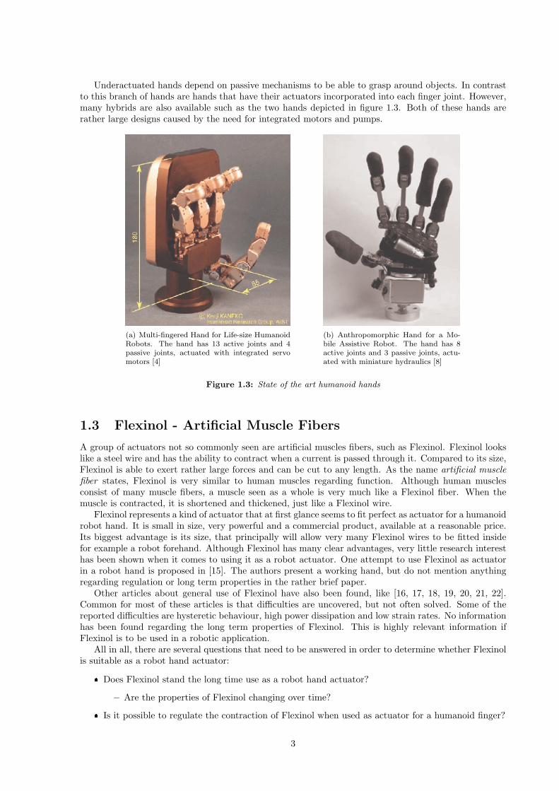
Underactuated hands depend on passive mechanisms to be able to grasp around objects. In contrastto this branch of hands are hands that have their actuators incorporated into each finger joint. However,many hybrids are also available such as the two hands depicted in figure 1.3. Both of these hands arerather large designs caused by the need for integrated motors and pumps.

(a) Multi-fingered Hand for Life-size HumanoidRobots. The hand has 13 active joints and 4passive joints, actuated with integrated servomotors [4]

(b) Anthropomorphic Hand for a Mo-bile Assistive Robot. The hand has 8active joints and 3 passive joints, actu-ated with miniature hydraulics [8]

Figure 1.3: State of the art humanoid hands

1.3 Flexinol - Artificial Muscle Fibers

A group of actuators not so commonly seen are artificial muscles fibers, such as Flexinol. Flexinol lookslike a steel wire and has the ability to contract when a current is passed through it. Compared to its size,Flexinol is able to exert rather large forces and can be cut to any length. As the name artificial musclefiber states, Flexinol is very similar to human muscles regarding function. Although human musclesconsist of many muscle fibers, a muscle seen as a whole is very much like a Flexinol fiber. When themuscle is contracted, it is shortened and thickened, just like a Flexinol wire.

Flexinol represents a kind of actuator that at first glance seems to fit perfect as actuator for a humanoidrobot hand. It is small in size, very powerful and a commercial product, available at a reasonable price.Its biggest advantage is its size, that principally will allow very many Flexinol wires to be fitted insidefor example a robot forehand. Although Flexinol has many clear advantages, very little research interesthas been shown when it comes to using it as a robot actuator. One attempt to use Flexinol as actuatorin a robot hand is proposed in [15]. The authors present a working hand, but do not mention anythingregarding regulation or long term properties in the rather brief paper.

Other articles about general use of Flexinol have also been found, like [16, 17, 18, 19, 20, 21, 22].Common for most of these articles is that difficulties are uncovered, but not often solved. Some of thereported difficulties are hysteretic behaviour, high power dissipation and low strain rates. No informationhas been found regarding the long term properties of Flexinol. This is highly relevant information ifFlexinol is to be used in a robotic application.

All in all, there are several questions that need to be answered in order to determine whether Flexinolis suitable as a robot hand actuator:

Does Flexinol stand the long time use as a robot hand actuator?

– Are the properties of Flexinol changing over time?

Is it possible to regulate the contraction of Flexinol when used as actuator for a humanoid finger?

3

Is it possible to improve the strain rate of Flexinol?

Is it possible to use multiple Flexinol wires in parallel?

1.4 Thesis Overview

This thesis aims to answer the questions stated above. Chapter 2 contains background information aboutFlexinol and other actuator technologies. A brief overview of the anatomy of the human hand is given inaddition to actuators and feedback sensors. Chapter 3 contains information about two of the tools usedin the practical work of the thesis and chapter 4 describes the methods that were developed in order toanswer the above questions. Chapter 5 contains an evaluation of the proposed methods and a discussionaround regulation is found in chapter 6. Suggestions to future work is given in chapter 7 and finally,a conclusion is given in chapter 8. Following is a list over all the practical work completed during thisthesis.

Long term testing of Flexinol

– Building test frame– Molding weights– Design of amplifier circuit for force measurements– Calibration of force and displacment transducers– Design of driver circuit for Flexinol wires– Programming of measurement software

* Program for controlling Flexinol wires and collecting data* Web application for remote surveillance and data browsing* Matlab scripts for analyzing data

PWM-control of Flexinol wire

– Design of microcontroller circuit with RS232 remote interface– Programming microcontroller

* Command interpreter for RS232 commands* Calibration algorithm* Flexinol regulation algorithm

– Programming computer interface* Text mode for debugging purposes* Command mode for easy operation* Continuous mode for data visualization

Humanoid finger application

– 3D design of a humanoid finger with a torque free tendon routing scheme– Printing in ABS-plastic and assembly of the finger– Design, printing and assembly of radial displacement transducers– Design, printing, assembly and calibration of force sensor brackets– Design of micorcontroller circuit with sensor input and Flexinol driver– Expansion of command set for microcontroller to include control and feedback of three wires– Programming computer interface

* Reuse of computer interface from PWM-testing* Interface for the Microsoft Robotics Studio framework

Regulation methods

– Proportional regulation for PWM-control and finger joints– Manual regulation of one wire using a high frequency pwm motor driver

4

1.5 Short Conclusion

This thesis shows that the use of Flexinol as actuator for a robotic finger is feasible. Flexinol has manydisadvantages that have to be overcome such as a limited life, hysteresis behaviour, limited strain rateand degeneration of wires but it also has advantages. Flexinol exerts very large forces compared to itsown size and needs very little physical space in an application. Figure 1.4 shows a humanoid fingeractuated with Flexinol wires and a test frame for testing Flexinol wires. Both products were developedduring this thesis.

(a) Humanoid finger developed in this thesis. The finger is actuated with threeFlexinol artificial muscle fibers and controlled with a microcontroller

(b) A test frame was built to in-vestigate the long term propertiesof Flexinol

Figure 1.4: Two products of the thesis

5

6

Chapter 2

Background

In this chapter, the background theory for the thesis is presented. First, the human hand is brieflypresented to later be used as motivation for the development of a humanoid finger. Secondly, availabletraditional actuators and actuators based on intelligent materials are presented and compared. Finally,different feedback sensors suitable for displacement- and force measurements in robotic applications arediscussed.

2.1 Anatomy of The Human Hand

In this section some basic anatomical principles of the human hand are presented. The human handconsists of 4 fingers and a thumb and is the main organ for physical interaction with the environmentsurrounding the human body. A schematic of the bones in the human hand can be seen in figure 2.1.

Figure 2.1: Schematic drawing of a human hand. Carpals and Metacarpals form the wrist and palm of the handwhile Proximal, Intermediate and Distal phalanges form the fingers

2.1.1 Skeleton

In figure 2.1, the carpals are known as the wrist and the metacarpals as the palm. Proximal, intermediateand distal phalanges form the three segments of the finger. The anatomy of the thumb and the wrist are

7

left out of this thesis as they are complex topics that are not needed for the presented work.

Metacarpal Phalanx

The metacarpal phalanx (yellow) is connected to the first finger segment (proximal phalanx) with ajoint called the metacarpophalangeal joint (MCP-joint). The MCP-joint is able to perform to types ofmovement, flexion/extension and abduction/adduction. Flexion in this case means bending the fingerwhile extension means extending the finger. Abduction denotes the sideways motion of the finger awayfrom the midline of the hand. The opposite movement, adduction, means moving the finger back againstthe midline of the hand.

Proximal Phalanx

The proximal phalanx (green) is connected to the metacarpal phalanx through the MCP-joint. On theother side of the finger segment it is connected to the second finger segment (intermediate phalanx) witha joint called the proximal interphalangeal joint (PIP-joint). The PIP-joint only has one axis of motionand is therefore called a hinge joint. Flexion and extension of the PIP-joint means bending and stretchingthe first finger joint.

Intermediate and Distal Phalanx

The intermediate (blue) and distal (red) phalanges are the middle and outer segments of the finger,respectively. They are connected with the distal interphalangeal joint (DIP-joint) which is a hinge jointlike the PIP-joint.

2.1.2 Tendons and Muscles

The actuating mechanism of the human body is represented by muscles. However, the forces needed togrip heavy objects are so large that the muscles needed cannot be fitted inside the human hand. Instead,the muscles are placed in the forearm and the forces exerted by the muscles are transferred to the handusing tendons. This type of muscle placement is called extrinsic [23]. The efficiency of a human muscleis reported to be between 14% and 27% in the context of rowing and cycling [24].

Human Skeletal Muscles

A skeletal muscle is fastened to a bone in the human body to cause movement and force exertion [24].Thus can it be seen as an actuator for the body. The muscle itself is a bundle of single, parallel musclefibers that are built up from muscle cells. A muscle cell consists of plates that are moved relative to eachother to generate motion. The cells cause the muscle fibers and the muscle to contract when it receivesa neural pulse, called an action potential. The frequency of the neural signal reception decides thecontraction rate and force of the muscle. The neural control signals for human skeletal muscle movementcan therefore be called pulse frequency modulated.

Finger Movement

The tendons and muscles responsible for flexion and extension of the finger are depicted in figure 2.2. Themost important parts for this thesis (marked with red) are the M. lumbricalis that flexes the MCP-joint,the M. flexor digitorum superficialis, Tendo that flexes the PIP-joint, the M. flexor digitorum profundus,Tendo that flexes the DIP-joint, and finally the M. extensor indicis, Tendo that extends the finger. Infigure 2.3, the insertion points of all the tendons in the hand can be observed.

2.1.3 Robotic Approach to the Human Hand

There are several aspects of the human hand that makes it very hard to imitate in a robotic application.First of all, the human hand has a very complex kinematic model. The fingers alone possess 21 degreesof freedom (DoF) according to [26]. In addition to the finger, movement of the palm includes 6 DoF,27 for the whole hand. The movement of the palm itself is rarely seen in robotic hands, a solid palm isoften used instead. In addition to the high degree of freedom, the finger is also very sensitive to external

8

Figure 2.2: Tendon routing in the human finger [25]. The most important tendons and muscles are marked withred

input. To imitate all the nerves on the surface of the finger is very complicated. Normally, a number oftouch sensors is seen instead.

2.2 Traditional Actuators

This section focuses on traditional actuators suitable for robotic applications.

2.2.1 Hydraulics

A widely used form of general actuation is hydraulic systems. A hydraulic system, which is depictedin figure 2.4, typically consists of a pump, a reservoir, a valve and an actuator. The hydraulic pumpis responsible for creating pressure by forcing liquid (typically oil) from the reservoir into the hydraulicsystem. By opening the valve, the pressurized liquid flows into the actuator, normally a hydraulic cylinder,creating movement. Depending on the physical characteristics of the pump and the actuator, the actuatorexerts a force as illustrated in figure 2.5. In this example, the input energy is supplied by the pump,whereas the output force is the actuation of the cylinder.

Hydraulic systems have been used commercially since the industrial revolution wherever great forceshave been needed. Traditionally, these systems have been quite large, not suitable for robotic applications.However, with development in technology, small systems including a micropump, valves and actuatorsnow may be integrated into the palm of a robotic hand [28].

2.2.2 Pneumatics

In pneumatics, a pressurized gas is used to create actuation, typically by filling a cylinder with air.In normal pneumatic systems a motion speed of up to 1m/s is obtained, but in high speed pneumaticsystems, speeds of 15m/s may be reached [29]. Figure 2.6 shows a pneumatic cylinder half full of air.Pneumatic cylinders can be either two way, as shown in the figure, or one way. A two way cylinder isactuated actively both ways with pressurized air in front of or behind the piston. A one way cylinder isreturned passively by a spring mechanism. By controlling the air flowing into the cylinder, the pistoncan be actuated to either end of the cylinder. Pneumatic systems can be very simple, containing only acompressor, valves and a cylinder. However, the efficiency of the compressor is low, causing an unwantedloss of power in for example mobile applications.

Pneumatic Artificial Muscles (PAMs)

PAMs [30] are special variants of pneumatic actuators. Figure 2.7 depicts a PAM in three different states.The muscle consists of a flexible membrane which can be filled with air. When the muscle is empty (a),

9

Figure 2.3: Insertion points on the human hand [25]. The blue dots show the three points essential for fingerflexion

the muscle is at its maximum length. When air is filled into the muscle, a pressure builds up causing thevolume to increase. As figure (b) shows, this decreases the length of the muscle. By further increase ofthe pressure the muscle reaches its maximum volume in (c). At this point the contraction of the musclecan be about 30% of its initial length. Many variants of PAMs are described in [30], but common for allis that they are light weighted. However, the use of PAMs has not been very common due to problemsregarding short life of the membrane caused by mechanical stress and friction forces. This seems to havechanged over the last decade as for example the Shadow Hand C5 [7] is actuated by a high number ofPAMs. Accurate control of the muscle has been reported to be non-trivial.

2.2.3 Servo Motors

A servo motor (figure 2.8) is a closed system which gets input information and performs a motionaccordingly. The input is typically a position or a velocity, but may also be information from a forcesensor or any other feedback sensor. Servo motors come in a variety of sizes, making them suitable formany different applications with different design considerations such as high force, small size or highspeed.

RC-Servo Motors

A subgroup of servo motors are servo motors for radio controlled (RC) applications. These motorstypically allow about 180-210 degrees of angular motion and are controlled with a pulse width modulated(PWM) signal with fixed frequency and varying duty cycle. A controller for such a signal can easilybe built in hardware or software. RC-servos come in different sizes and types, an example of a servofor robotic applications is given in figure 2.8. This servo has an idle wheel on the opposite side of thedrive wheel, making it suitable for stable assembly inside a joint. From leading manufacturer Hitec RCD(www.hitecrcd.com), the smallest available RC-servo (HS-35HD) [31] is 1.85cm× 0.76cm× 1.54cm and

10

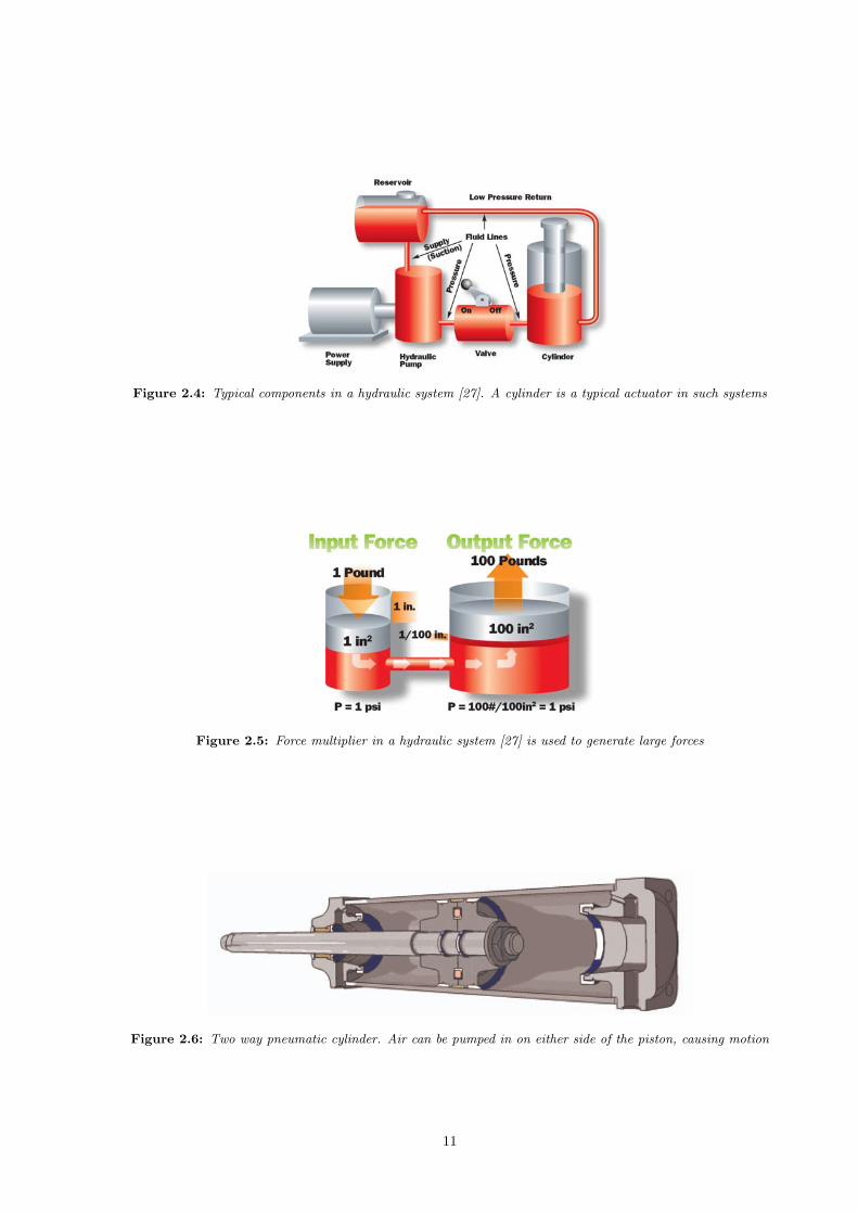
Figure 2.4: Typical components in a hydraulic system [27]. A cylinder is a typical actuator in such systems

Figure 2.5: Force multiplier in a hydraulic system [27] is used to generate large forces

Figure 2.6: Two way pneumatic cylinder. Air can be pumped in on either side of the piston, causing motion

11

Figure 2.7: Pneumatic artificial muscle [30]. When air is pumped into the membrane, it is shortened, causingmotion

has a torque of 10Ncm. The biggest servo (HS-815BB) is 6.58cm× 3.00cm× 5.74cm and has a torque of242Ncm.

The biggest advantage of servo motors is their very easy control. Typically, a RC-servo takes a PWM-signal with a period of 20ms (50Hz). With a duty cycle of 1.5ms

20ms the servo is in its center position. Byincreasing the duty cycle to 2ms

20ms or decreasing it to 1ms20ms the servo is moving respectively +90 or −90.

Figure 2.8: Robot servo motor from Hitec [32]. The servo has an idle wheel for assembly inside for example arobot joint

2.2.4 Stepper Motors

Stepper motors create angular motion, just as servo motors do. As the servo motor uses feedback tocontrol its position or speed, the stepper motor has no need for this. To eliminate the need for feedback,the stepper motor divides one turn of the motor into a fixed number of steps, varying from model tomodel. The simplest form of a stepper motor can be seen in figure 2.9. The drive shaft is fastened inthe toothed wheel which is surrounded by four electromagnets with toothed surfaces. In step 1, the topmagnet is turned on, making the teeth of the wheel align with this magnets teeth. The right magnetis positioned with an angular offset from the top magnet with 1

4 of the angle between two teeth on thewheel. When turning the top magnet off and the right magnet on (step 2), the teeth of the wheel willalign with the teeth of the right magnet, causing a motion with 1

4 of the tooth angle. Step 3 involvesturning the right magnet off and the bottom magnet on, causing another step of motion. In step 4,the bottom magnet is turned off and the left magnet is turned on. The wheel has now turned 3

4 of thetooth angle and the next time step 1 is enabled, the wheel has moved by 1 tooth angle. In this way, the

12

motion of the wheel can be controlled very freely. Other variants of step control is more common thanthis example, involving more than one magnet turned on at a time.

Stepper motors can produce very high torques at low speeds. However, at higher speeds the motorloses some of its torque. At lower speeds, the stepping of the motor can cause mechanical vibrationswhich in some applications are unwanted. There is also a possibility that the motor can lose steps whenheavily loaded. This will cause the controller to believe that the motor has moved one step when it inreality may have stood still. To prevent this, some models include an angular feedback from the motorshaft.

(a) Step 1 (b) Step 2 (c) Step 3 (d) Step 4

Figure 2.9: Fundamental operation of a stepper motor. After four steps, the drive shaft has turned one toothclockwise

2.2.5 Electric Solenoids

Electric solenoid actuators are based on magnetic forces. An example of a commercial solenoid actuatorcan be seen in figure 2.10. A coil is situated around the stem of the actuator. When alternating currentis passed through the coil, a magnetic field builds up, and the stem is attracted towards the center ofthe coil. When the current stops, the stem is free and can be moved back either by active force or by areturn spring.

An advantage of solenoid actuators in comparison to pneumatic and hydraulic actuators is easyinstallation and the fact that no reservoir of fluid or air is needed. A disadvantage of solenoids is thatthey only have two positions when actuated, either on or off. As the stem is pulled into center of thecoil, the force increases, leading to a varying force exertion during the actuation period. By examiningdatasheets [33, 34] from manufacturers Ledex (www.ledex.com) and Dialight BLP (www.blpcomp.com) itseems that the maximum force of available actuators is about 650N. However, a solenoid that exerts sucha large force has the disadvantage that it weights over 2.2kg. The speed of the solenoid actuator dependsgreatly on the force it is set to exert. When unloaded, an actuation can be performed in less than 50ms[33, 34] in most cases. When operated, heat is dissipated in the solenoid which modifies the characteristicsof it. Typically, the speed of the actuator stroke and the maximum force is at their maximum when theduty cycle of the solenoid is low, meaning the actuator gets to cool down between each actuation.

2.3 Intelligent Materials used as Actuators

In this section, several different actuators, based on intelligent materials, are presented. Intelligentmaterials used as actuators are subject for research and not yet commonly seen in real life applications.Common for most of these technologies is that they often have at least one big drawback, making themnon-trivial in use. This section gives a presentation of different actuators and references to researchperformed in the area.

2.3.1 Shape Memory Alloys in General

Shape memory alloys (SMAs) are a group of alloys that possesses the shape memory effect (SME) [19].This section focuses on the nickel-titanium (NiTi) alloy, which appears to be the most commonly usedalloy. The shape memory effect is a temperature dependent transformation between to phases, martensite

13

(a) Push type (b) Pull type

Figure 2.10: Ledex ® Electric Solenoid Actuator [33] Operation. Magnetic force is used to drive the stem intoor out of the housing

and austenite, which is illustrated in figure 2.11. The martensite phase is also known as the cold phase ofthe material, normally occurring at room temperature. Although this phase may appear as the originalphase of the material, it is really the phase in which the material is deformed. This is according tothe internal crystalline structure of the material, which at this point is stretched (figure 2.11c). Byapplying heat to the material (figure 2.12a), a transformation from martensite to austenite starts at thetemperature Astart. Further heating of the material leads to a straightening of the crystalline structureuntil the temperature Afinish is reached. The material is now in its austenite phase, with its crystallinestructure in its original state (figure 2.11a). When cooling the material, the transformation from austeniteback to the martensite phase starts at temperature Mstart and ends at temperature Mfinish (figure 2.11b).Cooling of the material alone does not make the material go back to its martensite shape, stress alsohas to be applied to the material to stretch the internal crystalline structure (figure 2.11c). Figure 2.12bshows the same transformation curve as figure 2.12a, but also has stress as a parameter. As can beseen, applying stress to the SMA-material leads to a shifting of the transformation curve. Higher stressmeans that a higher temperature is needed to reach the austenite phase, and vice versa is the martensitephase reached at a higher temperature than when no stress is applied. A hysteresis behaviour can alsobe observed between the heating and cooling phase in both cases. More on hysteretic behaviour can befound in [16].

Figure 2.11: Cycle of the Shape Memory Effect [35]. The grid symbolizes the atomic crystalline structure of thematerial

14

(a) Temperature hysteresis (b) Temperature hysteresis and stress

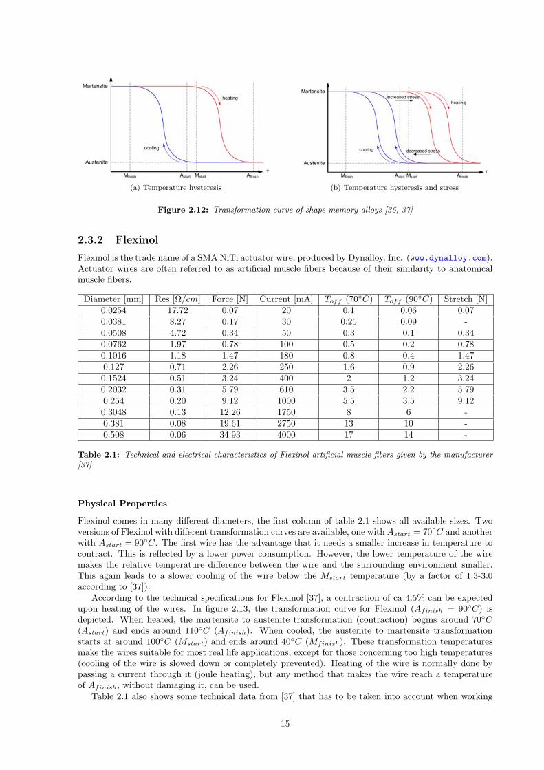
Figure 2.12: Transformation curve of shape memory alloys [36, 37]

2.3.2 Flexinol

Flexinol is the trade name of a SMA NiTi actuator wire, produced by Dynalloy, Inc. (www.dynalloy.com).Actuator wires are often referred to as artificial muscle fibers because of their similarity to anatomicalmuscle fibers.

Diameter [mm] Res [Ω/cm] Force [N] Current [mA] Toff (70C) Toff (90C) Stretch [N]0.0254 17.72 0.07 20 0.1 0.06 0.070.0381 8.27 0.17 30 0.25 0.09 -0.0508 4.72 0.34 50 0.3 0.1 0.340.0762 1.97 0.78 100 0.5 0.2 0.780.1016 1.18 1.47 180 0.8 0.4 1.470.127 0.71 2.26 250 1.6 0.9 2.260.1524 0.51 3.24 400 2 1.2 3.240.2032 0.31 5.79 610 3.5 2.2 5.790.254 0.20 9.12 1000 5.5 3.5 9.120.3048 0.13 12.26 1750 8 6 -0.381 0.08 19.61 2750 13 10 -0.508 0.06 34.93 4000 17 14 -

Table 2.1: Technical and electrical characteristics of Flexinol artificial muscle fibers given by the manufacturer[37]

Physical Properties

Flexinol comes in many different diameters, the first column of table 2.1 shows all available sizes. Twoversions of Flexinol with different transformation curves are available, one with Astart = 70C and anotherwith Astart = 90C. The first wire has the advantage that it needs a smaller increase in temperature tocontract. This is reflected by a lower power consumption. However, the lower temperature of the wiremakes the relative temperature difference between the wire and the surrounding environment smaller.This again leads to a slower cooling of the wire below the Mstart temperature (by a factor of 1.3-3.0according to [37]).

According to the technical specifications for Flexinol [37], a contraction of ca 4.5% can be expectedupon heating of the wires. In figure 2.13, the transformation curve for Flexinol (Afinish = 90C) isdepicted. When heated, the martensite to austenite transformation (contraction) begins around 70C(Astart) and ends around 110C (Afinish). When cooled, the austenite to martensite transformationstarts at around 100C (Mstart) and ends around 40C (Mfinish). These transformation temperaturesmake the wires suitable for most real life applications, except for those concerning too high temperatures(cooling of the wire is slowed down or completely prevented). Heating of the wire is normally done bypassing a current through it (joule heating), but any method that makes the wire reach a temperatureof Afinish, without damaging it, can be used.

Table 2.1 also shows some technical data from [37] that has to be taken into account when working

15

Figure 2.13: Transformation curve of Flexinol [37]. Relatively large changes in strain are observed between 85Cand 95C

with Flexinol. The first column of table 2.1 contains the different wire diameters. The diameter of thewire determines its resistance and maximal pull force, found in column 2 and 3. A Flexinol wire has aspecified resistance according to the length and diameter of it. The specified current in the table is thecurrent needed to heat the wire above its transition temperature in one second. More about the timeresponse of Flexinol can be found in [20]. The voltage U , needed to create such a current can easily becalculated using Ohm’s law, U = RI, where R is the resistance of the wire, measured or calculated fromits length, and where I is the wanted current. Generally, resistive materials have an increase in resistancewhen heated. This does not apply to Flexinol in the same way due to the fact that the shape of the wirechanges as a function of temperature. The volume of the wire is constant at all times, leading to a largerdiameter and smaller length in the austenite phase compared to in the martensite phase. The formula fora materials resistance R is given as R = ρ·l

A , where ρ is the specific electrical resistivity of the material, lis the length of the material and A is the cross-sectional area of the material. From the formula it is clearthat by shortening and thickening the wire, the resistance is decreased. This assumption holds becausethe increase in ρ caused by temperature is negligible compared to the decrease in resistance caused bydeformation.

The pull force found in column 3 of table 2.1 is the maximum guaranteed pull force reported by themanufacturer. This means, that by exceeding the maximum pull force, a stable contraction rate overtime cannot be guaranteed. This should specially be taken in concern when designing the mechanicalparts of a system. An overloaded wire will most likely cause the need for a replacement - a drawback inmost applications.

As already mentioned, the current given in column 4 is the amount needed to contract the wire inone second, surrounded by air at room temperature. Of course, a smaller current than specified in thetable can be used. This leads to a slower contraction but also to a higher power consumption caused bythe increase in time that the warm material is exposed to its surrounding air. From the manufacturerof Flexinol, it is reported that any current waveform can be used to heat the wires. This makes thewires suitable for embedded solutions, using for example a widely common PWM module to controlthe contraction speed. Column 5 and 6 in table 2.1 show the cooling time for Flexinol wires withAstart = 70C and Astart = 90C surrounded by air at room temperature. The differences in coolingtime solely depend on the surface to volume ratio of the wires. The surface area of the wire has a lineargrowth when written as function of the diameter (A = π ·D). In comparison, the volume of the wire hasa quadratic growth (V = π · (D/2)2) and as a result, doubling the wire diameter results in more thana doubling of the cooling time. In applications where great force is needed, faster cooling times may beachieved by coupling multiple wires in parallel. This solution depends on that multiple Flexinol wires areable to work together in parallel and has the disadvantage that more space is needed. In [21], a designfor a Flexinol bundle is proposed (depicted in figure 2.14).

To shorten the cooling time, a number of different actions can be taken as shown in table 2.2. Theimprovement ratios in the table are given in the technical specifications for Flexinol [37]. Another coolingtechnique is discussed in [38].

The rightmost column in table 2.1 shows the force that is recommended to stretch a wire that has

16

(a) Crimping of the wires to the end plates (b) End plate for parallel wires. The number ofelectrical parallel connected wires can be used tocontrol the electrical operating point of the wires

Figure 2.14: A SMA Bundle Actuator [21]. By using many parallel wires, very large forces can be exerted

Method ImprovementStill air 1:1Increasing stress 1.2:1Using higher temperature wire 2:1Using solid heat sink materials 2:1Forced air 4:1Heat conductive grease 10:1Oil immersion 25:1Water with glycol 100:1

Table 2.2: Cooling techniques [37]. The improvement is the increase in cooling rate when the correspondingcooling technique is applied

17

been contracted. The numbers are provided by the manufacturers of Flexinol.In figure 2.15a, a drive circuit schematic for a Flexinol wire can be seen. The current flowing through

the wire is controlled by the power MOSFET, directly connected to a power supply. A precision resistorconnected between the wire and ground is used for current measurements. The resistor should be smallenough to build up only a minimal voltage, relative to the drive voltage of the wire. The use of a pMOStransistor may seem strange because a nMOS normally has better driving characteristics. However, forthe small signal driver it is desirable with a positive control signal for safety reasons. An undriven oruninitialized control signal should not cause a wire contraction or a current flow as this could be dangerousin for example a robot application that interacts with humans.

(a) Normal driver circuit. Charging of thetransistor may draw currents ≥ 20mA

(b) Small signal driver circuit. Suitable in for exam-ple microcontroller applications

Figure 2.15: Circuits for driving Flexinol wires (blue)

Precautions

The contraction speed of the wire is reported to be proportional to the current used to heat it. However,concern should be taken, not to overheat or overload the wire. A too high temperature or a too highstress will cause permanent damage to the wire, reducing its ability to contract [37]. The manufacturerhas not reported any detailed specifications other than a general warning. Stretching of the material isnormally done using a spring or a dead weight. Although the strain percentage of Flexinol is reportedto be maximal 5%, the maximal strain percentage of the NiTi alloy is 8% [39]. In practice, this meansthat from its austenite phase, the wire can be stretched 8% without causing any damage to its crystallinestructure. By violating this limit, permanent damage is done to the wire, decreasing its maximum strainrate.

Control

In many applications, it is desirable to control the contraction of the wire somewhere between no con-traction and maximum contraction. As figure 2.12b shows, the transformation curve shifts according toapplied stress, making such a control of the contraction rate non-trivial. Theoretically this could be doneby measuring the current passing through the wire, as mentioned above. However, no research has beenfound confirming this assumption.

In [17], a method for controlling the degree of contraction is proposed. The authors heat and cool theFlexinol wire with the use of Peltier elements. Peltier elements are electrically driven heaters and coolers.When passing a current through the element, a temperature difference builds up between the warm andcold side of the element. By applying a heat sink to the cold side, high temperatures may be built upon the warm side of the element. By reversing the current, the warm side becomes cold and vice versa[40]. The authors use several elements to heat the different segments of a Flexinol wire, as illustrated infigure 2.16a. Every single Peltier element is controlled in a binary manner, set to either heat or cool itscorresponding wire segment. In this way, by deciding how many Peltier elements that cool the wire and

18

how many that heat the wire, the degree of contraction of the wire can be controlled. The assembly ofPeltier elements on a Flexinol wire is depicted in figure 2.16b.

By looking at commercial Peltier elements [41, 42], it can be concluded that heating and coolingrequires more power than normal joule heating does when controlling a Flexinol wire. What has tobe taken into consideration when applying Peltier elements to an application is the increase in systemcomplexity. The biggest disadvantage by introducing Peltier elements to control Flexinol wires, is theincreased physical space needed for each wire. By increasing the space need for an application, the biggestadvantage of Flexinol, its weight to force ratio, is removed.

(a) Segmentation of the wire. By reg-ulating each segment to a hot or coldstate, the total amount of contractioncan be controlled

(b) Assembly of a Peltier element on a Flexinol wire. The result isa large increase in physical size

Figure 2.16: Binary control of segmented Flexinol wire [17]

Movement

One drawback of Flexinol wires is their limited strain rate. Under normal conditions, a strain rate of4.5% can be expected, which in many applications means that very long wires have to been used in orderto generate the needed amount of movement. The most elegant and easy way to use Flexinol is to connectone wire that generates exact the amount of desired force and movement. In many real life application,this cannot be expected due to space limitations and force needs. Therefore, different mechanical gearmechanisms have been proposed to overcome this problem. The gear mechanisms shown in figure 2.17are from the makers of Flexinol [37]. Figure 2.17a shows an angle pull of a Flexinol wire (blue line), wherethe displacement ratio is given by the formula δd

δs = 1sin(α) . Here, δd is the contraction of the wire and δs

is the output movement of the gear. The formula shows that a decrease of the angle α leads to a higherratio, the ratio is in other words variable over the working range of the gear. The force transmission isalso affected by the gear and can be written as Fs = Fd · cos(γ), where Fs is the output force of the gearand Fd is the force generated by Flexinol. As expected, an increase in stroke length leads to a decreasein force. Figure 2.17b shows a second gear variant which makes use of a lever mechanism. The lever(red bar) has a defined pivot point L1/L2 from one end. The displacement ratio of the gear is linearlydependent on the relationship between L1 and L2 and can be written as δd

δs = L1L2 . The force ratio is

inverse of the displacement ratio and is written as Fs = Fd·L1L2 . Figure 2.17c shows a radial pull which

is similar to the anatomical principals of tendon fastening in the human body. The displacement of thegear is written as δd

δs = r1r2

and the output force as Fs = Fd · cos(α).Another gear mechanism is reported in [22] and can be seen in figure 2.18 and 2.19. The author

introduces a special routing scheme in a pattern around multiple gear plates (figure 2.18b and 2.19a) andmakes use of the angle pull from figure 2.17a. A loss of force due to friction and deformation is observed,but in exchange the author is able to get a strain rate of 18%. However, the size of the gear makes theapplication gigantic compared to a single Flexinol wire.

Commercial Applications

Although Flexinol and similar products have been available on the market for several years, it does notseem like a particular brand of applications have been pointed out as very suitable. Not many examples

19

(a) Angle pull (b) Lever (c) Radial pull

Figure 2.17: Gear mechanisms for Flexinol [37]. The gears result in larger strains and lower forces

(a) Gear plates are pulled against each other (b) Gear assembly. The number of gear platesdecides the strain rate

Figure 2.18: SMA actuator with high strain [22]. Proposition unfortunately results in a large increase in physicalsize

(a) Wire routing schematic. The wires are routedin a diagonal pattern around the gear structure

(b) Top view and side view of the gear. The rout-ing tracks can be seen on the top of the gear plate

Figure 2.19: SMA actuator with high strain [22]

20

have been found on commercial applications that use Flexinol, and the ones found may appear to beproduced by Dynalloy, Inc. An example for one of these products is the ElectrostemTM air valve [43].The air valve has been made to give a practical example of the possibilities of Flexinol. The rather simpledesign of the air valve can be seen in figure 2.20.

Figure 2.20: The Flexinol ElectrostemTM air valve [43]. The valve uses the thermal properties of Flexinol toregulate air flow

The valve is said to be able to proportionally control the air flowing through it. The valve itself isa standard car tyre valve (Schrader valve) which is controlled by its internal stem cap as seen in figure2.21. As figure 2.20 shows, the Flexinol wire is fastened internally on the stem cap of the ElectrostemTM

valve. When contracting the wire, the valve opens and air flows through it. This operation itself isnot very special compared to other electrically driven air valves except for the small size of the valve.However, as air flows through the valve, one of the special characteristics of Flexinol is revealed. Theair flow cools the Flexinol wire down, working against the Joule heating of the wire. With an increasingpressure difference between the inside and the outside of the valve, the amount of air flowing through thevalve also increases. The wire is further cooled causing the valve to decrease the air flow until a balancebetween heating and cooling of the wire stabilizes.

The wire needs about 750mA to operate, but if a higher air flow is wanted, the current may beincreased. However, if the current is increased and the airflow suddenly stops, the wire and the valvecould very fast overheat causing permanent damage. The danger of overheating is generally a reoccurringchallenge when using Flexinol, and should always be taken into concern when designing applications.

Non-Commercial Applications

The small six-legged robot bug Stiquito can be found in [44, 45]. The robot bug is able to walk 10centimeters per minute and carry a load of 50g. It uses Flexinol wires of 100µm to move its legs. Otherscientific applications are presented in [46, 47].

(a) Schradervalve closed

(b) Schradervalve open

Figure 2.21: Schrader valve operation which can be handled by a Flexinol wire

21

2.3.3 Electroactive Polymers

Electroactive polymers (EAP) are a group of polymer materials that change their shape as a result of anapplied voltage [48]. Electroactive polymers can be divided into two groups, whereas the first group areelectroactive polymers that can be operated in a dry environment. The other group consists of polymersthat need to be wet in order to function. Common for all EAP-materials is that large strain rates canbe expected when compared to for example shape memory alloys. However, the exerted force is muchlower than that of SMAs - one of the biggest drawbacks of EAPs. Examples of EAP applications can befound in [49, 50, 51, 52, 53, 54]. Figure 2.22 and 2.23 show two underwater applications actuated withfins built from EAP materials.

Figure 2.22: Underwater micro robot that is actuated with a ICPF (Ionic conducting polymer film) fin [55].

(a) Deformation mechanics of IPMC (Ionicpolymer-metal composite) [50]. When a voltageis applied, the water in the material moves to oneside, causing a bending of the material.

(b) A fin construction for a Rajiform SwimmingRobot [50]. EAP technologies that need a wet en-vironment are well suited for underwater applica-tions.

Figure 2.23: EAP technology

2.4 Actuator Comparison

In this section a comparison between the mentioned actuators is done. Table 2.3 shows a summary of theresults. As more and more manufacturers enter the market, it gets harder and harder to get a generalview of the available products. In many applications it is not easy to decide what actuator technology

22

to use, as many technologies share some of their properties. A deep analysis of the actual actuator needis therefore crucial to make a good decision.

Flexinol and electroactive polymers differ from the other actuators in being very small in size and inbeing non-mature technologies. Flexinol is able to exert great forces and has a high power to weight ratio[56], but suffers from small strain rates, that can be compensated with gears. Electroactive polymerscan be said to have opposite properties with large strain rates but only exert small forces. Electroactivepolymers in some cases need drive voltages of ≥ 1000V.

Hydraulics have been used for a long time and a wide number of parts in different sizes are thereforeavailable. Lately, very small systems have also been developed. Tremendous forces can be achieved usinghydraulics, at the cost of heavy systems. As a result of technology development, pneumatics are moreand more used in robotics in the form of PAMs. These systems are in general lighter than hydraulicsystems, but the exerted forces are lower when compared against the system weight.

Radial movement is often achieved by RC servos or stepper motors. For example are RC servos idealfor actuating a joint with a given degree of movement, while a stepper motor would better be fitted inan application driving for example a multi-turn wheel. Both technologies seem to create about the sameamount of torque, but stepper motors have the disadvantage that they lose power as the motor speedincreases. On the other hand, RC servos tend to be rather slow compared to stepper motors, caused bytheir internal gears. Stepper motors normally do not need gears.

Solenoids are normally used to operate valves, but may also be used in robotic applications. However,as only to positions are available when actuating, the number of suitable applications are rather low.

Actuator Motion Force Size Res. Control Strain RefFlexinol(SMA)

Linear 40N Small high Non-trivial 4.5% [37]

Electroactivepolymers

Linear Weak Small high Non-trivial ≤ 120% [35]

Hydraulics Linear Strong Med/Large high Controller - [27, 28]Pneumatics Linear Medium Med/Large On/Off Controller - [29]PAM Linear Medium Medium high Controller 30% [30]RC Servomotors

Radial ca 250Ncm Medium ca 1 PWM ±90 [31]

Stepper mo-tors

Radial ca 300Ncm Medium ca 0.5 Controller - [57]

ElectricSolenoids

Linear 150N Medium On/Off Binary - [33]

Table 2.3: Comparison of different actuators and some of their properties

2.4.1 Power to Weight Ratio

Figure 2.24 shows the power-to-weight ratio [58] of the above mentioned actuator technologies. Valuesfor SMAs, hydraulics, pneumatics and DC-motors were found in [35, 59, 60]. Values for EAP actuatorsare based on numbers found in [61, 62]. For electronic solenoids, no exact numbers were found. Thevalues in the figure is therefore based on one of the smallest and one of the largest solenoids from Ledex[63, 64]. To calculate the effect, an assumption was made that the actuation time for the solenoid is onesecond which is considered a reasonable actuating time in robotic applications.

The actuation time that is used to calculate the effect is a factor that has to be considered whencomparing the power-to-weight ratio of all technologies. Lately, very small DC-motors and hydraulicshave become available. This comparison does not include such actuators.

2.5 Feedback Sensors

This section describes different types of feedback sensors suitable in a humanoid robot finger. Two maintypes are mentioned, sensors for displacement measurements and sensors for force measurements.

23

Figure 2.24: Power-to-weight ratio of different actuator technologies [35, 59, 60, 61, 62, 63, 64]

2.5.1 Displacement Transducers

In robotic applications, it is often desirable to know how much mechanical parts have been moved. Suchtasks are often solved with a displacement transducer.

Linear Variable Differential Transformers (LVDT)

A LVDT is in general a simple construction consisting of three coils and a sliding magnetic core. Figure2.25 shows a schematic and a layout view of a LVDT. The single red coil is driven with a fixed frequencyand fixed amplitude AC signal. The two secondary coils (green and blue) are connected in oppositedirections so that when the metal core is in the center position, the induced currents from the coils canceleach other. However, by moving the metal core away from the center position, a difference in the twosignals is measured according to the position of the core. By looking at the phase of the differential signalaccording to the signal present at the center coil, it can be determined whether the metal core is movedto the left or to the right of the center position.

The use of electromagnetism makes mechanical contact between the metal core and the coils unnec-essary. This has two great advantages. This means that very little wearing can be observed, causing along life. It also leads to clean data and almost infinite resolution. On the other hand, the use of LVDTsrequires a fixed frequency for the center coil. If a dc output is wanted, some simple signal processingalso has to be done externally. Some products like [65] have internal signal processing and frequencygeneration and only need DC power to be operated.

Resistive (potentiometric) Displacement Transducers

Compared to LVDTs, resistive displacement transducers are in general cheaper. They consist of a sliderthat is moved back and forth over the surface of a resistive material as figure 2.26 shows. The resistivematerial acts like a voltage divider, causing the output voltage to be proportional to the position of theslider. Resistive displacement transducers are widely used, but because of the contact between the slidingmechanism and the resistive material, their lifetime is in general shorter than that of a LVDT. A greatadvantage of resistive displacement transducers is the simple three wire connection. Any common supplyvoltage can be used as excitation and they can therefore easily be fitted into most applications.

24

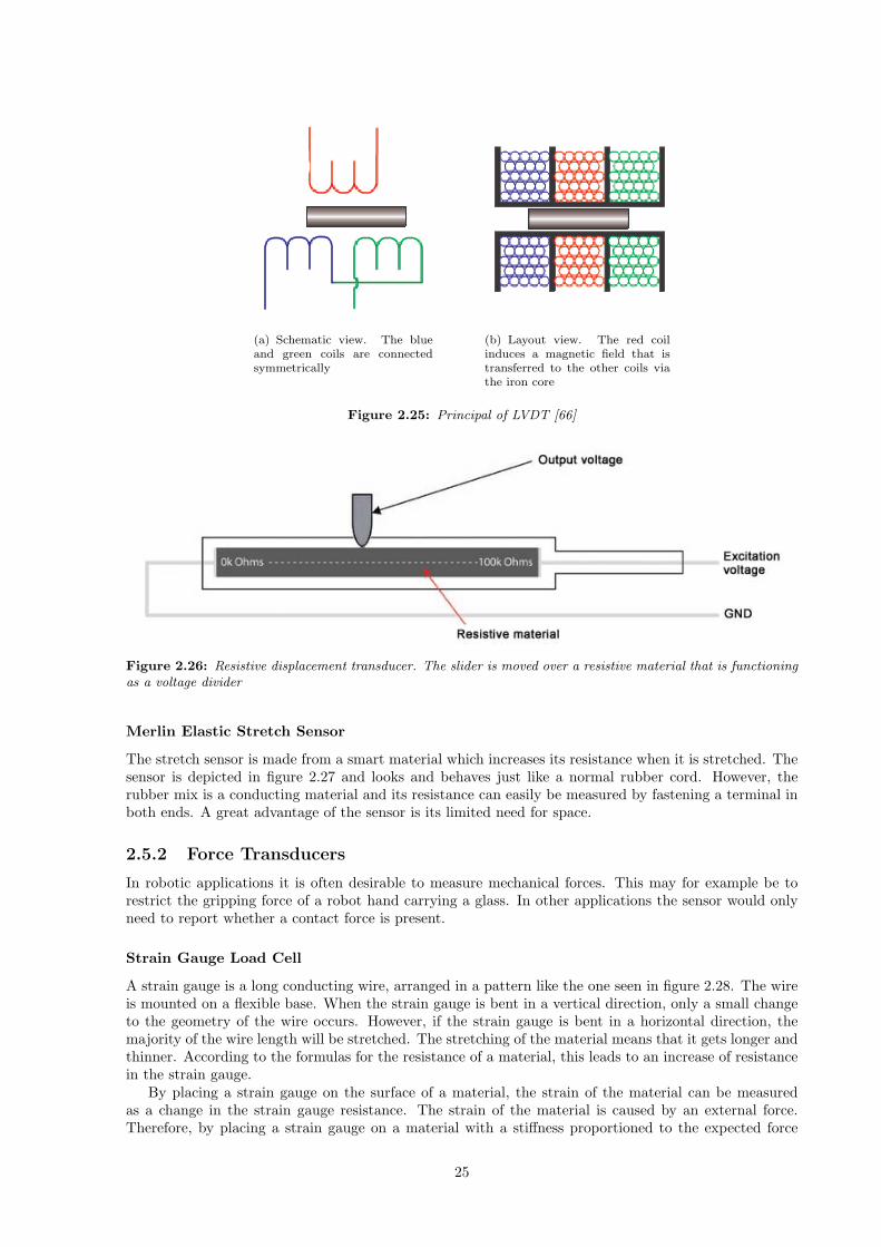
(a) Schematic view. The blueand green coils are connectedsymmetrically

(b) Layout view. The red coilinduces a magnetic field that istransferred to the other coils viathe iron core

Figure 2.25: Principal of LVDT [66]

Figure 2.26: Resistive displacement transducer. The slider is moved over a resistive material that is functioningas a voltage divider

Merlin Elastic Stretch Sensor

The stretch sensor is made from a smart material which increases its resistance when it is stretched. Thesensor is depicted in figure 2.27 and looks and behaves just like a normal rubber cord. However, therubber mix is a conducting material and its resistance can easily be measured by fastening a terminal inboth ends. A great advantage of the sensor is its limited need for space.

2.5.2 Force Transducers

In robotic applications it is often desirable to measure mechanical forces. This may for example be torestrict the gripping force of a robot hand carrying a glass. In other applications the sensor would onlyneed to report whether a contact force is present.

Strain Gauge Load Cell

A strain gauge is a long conducting wire, arranged in a pattern like the one seen in figure 2.28. The wireis mounted on a flexible base. When the strain gauge is bent in a vertical direction, only a small changeto the geometry of the wire occurs. However, if the strain gauge is bent in a horizontal direction, themajority of the wire length will be stretched. The stretching of the material means that it gets longer andthinner. According to the formulas for the resistance of a material, this leads to an increase of resistancein the strain gauge.

By placing a strain gauge on the surface of a material, the strain of the material can be measuredas a change in the strain gauge resistance. The strain of the material is caused by an external force.Therefore, by placing a strain gauge on a material with a stiffness proportioned to the expected force

25

Figure 2.27: The elastic stretch sensor from Merlin increases its resistance when it is stretched

Figure 2.28: Strain gauge. The zig-zag pattern makes the wire change its resistivity when stretched in a horizontaldirection

range, the exerted force can be measured as a change in strain. The material that the small strain gaugeis fastened on is in general much larger than the strain gauge itself. To measure the small changes instrain gauge resistance, a Wheatstone bridge is often used. Figure 2.29 depicts four strain gauges onthe surface of a material, connected as a Wheatstone full-bridge. As the figure shows, an increase ofresistance in R2 and R4 occurs when the material is bent. This unbalances the two voltage dividers ofthe Wheatstone bridge and causes a voltage difference between their two center nodes. The force causinga material strain is represented by this voltage.

Strain gauge load cells are specified with a maximum load and a sensitivity. The sensitivity of theload cell is reported as mV/V. This denotes the amount of millivolts per excitation volt the output ofthe Wheatstone bridge will be when the load cell is loaded to its maximum. For a load cell specified to100N and 2mV/V, an excitation voltage of 1V would cause an output of 2mV when the cell is loadedwith 100N. In the same way, with an excitation voltage of 10V the output would be 20mV.

Because of these low voltages, the use of a Wheatstone bridge is required. The differential measurementwill cancel noise that is present on both channels. Also, if only one voltage divider would have been used,the output voltage would be Vdd

2 ± 20mV . If a Vdd of 5V would be used, the output would thereforebe about 2.5V ±20mV . This would waste almost the hole measuring range of the data acquisitionunit. Instead, by introducing two balanced voltage dividers and measuring their difference, a much moreefficient use of the measuring range is achieved (0V ±20mV ). Another great advantage of the Wheatstonebridge is its ability to cancel temperature drifts. This is caused by the mirrored placement of resistorslike R2 and R4 in figure 2.29.

Interlink Force Sensing Resistor [67]

The Interlink Force Sensing Resistor (FSR) is not designed for accurate force measurements, but canbe used for indications. The FSR decreases its resistance as stress is applied to its polymer material.This behaviour is known as the piezoresistive effect. Although the accuracy of the FSR is reported to berather poor, its physical size of ca 8mm · 1mm (figure 2.30) makes it ideal for robotic use. In contrast,strain gauge load cells tend to be very large. A great advantage of the FSR is its high sensitivity. Asmall change in pressure causes the resistance of the sensor to change with many hundred Ohm. Thiseliminates the need for an amplifier.

26

Figure 2.29: Strain gauge connected as Wheatstone bridge. Very small changes in resistivity can be measured

Figure 2.30: Interlink Force Sensing Resistor [67]. Small changes in pressure result in large changes in resistivity

27

28

Chapter 3

Used Tools

In this chapter, three essential development tools are presented. First, the Atmel ATMega32 microcon-troller is described. The ATMega32 will later be used to implement a control unit for a humanoid finger.Secondly, the data acquisition unit for the later described test frame is described and finally, an overviewof the robotic software framework, Microsoft Robotics Studio, is given. An interface for Robotics Studiowill later be developed for a humanoid finger.

3.1 Atmel AVR Microcontrollers

The 8bit AVR microcontrollers from manufacturer Atmel (www.atmel.com) are a series of RISC-controllerswith high performance and low power consumption. They have a Harvard architecture (figure 3.1) andcan be operated at clock frequencies up to 20MHz. Code development, compiling and simulation canbe done in Atmels own AVR Studio, which also handles uploading the compiled microprogram to theflash memory of the microcontroller. This can be done via the microcontrollers In System Programming(ISP) interface, Jont Test Action Group (JTAG)interface or High Voltage Serial Programming (HVSP)interface. This section focuses on the AVR ATMega32 device [68], but the information is also highlyrelevant for other AVR devices as all of these are built upon the same AVR hardware platform.

The ATMega32 has a wide range of integrated functions for internal and external operations. Thisis a presentation of the most important functions used in this thesis. Generally, all functions in themicrocontroller are controlled by setting bits in the corresponding control registers of the function.

3.1.1 I/O-Ports

The microcontroller has many different I/O-ports, the number depends on the chosen housing. All portscan be used as general digital inputs or outputs and in addition most ports can be configured to performone or more other functions. The pinout of the ATMega32 in a PDIP-40 housing can be seen in figure3.2. The pin names written within a parenthesis are the alternate functions of each pin.

When a port is used as a normal digital input or output pin, the direction of the signal has to beconfigured. This is done by writing respectively a ’1’ or a ’0’ in the data direction register (DDR) ofthe port. When used as input, an internal pull-up of the pin is done, making the use of external activelow signals convenient. The alternate functions of a port is configured through the control register of thefunction. Some of these functions are described below.

3.1.2 Memory

The ATMega32 has 32kB of internal non-volatile flash memory for program code. Additionally, themicrocontroller has 2kB of SRAM used for data variables and 1kB of EEPROM for data storage. TheSRAM is volatile, meaning its state gets lost on a shutdown of the microcontroller. The EEPROM isnon-volatile and supports 100,000 write cycles, making it very suitable for storing device setup or mediumsized datasets.

29

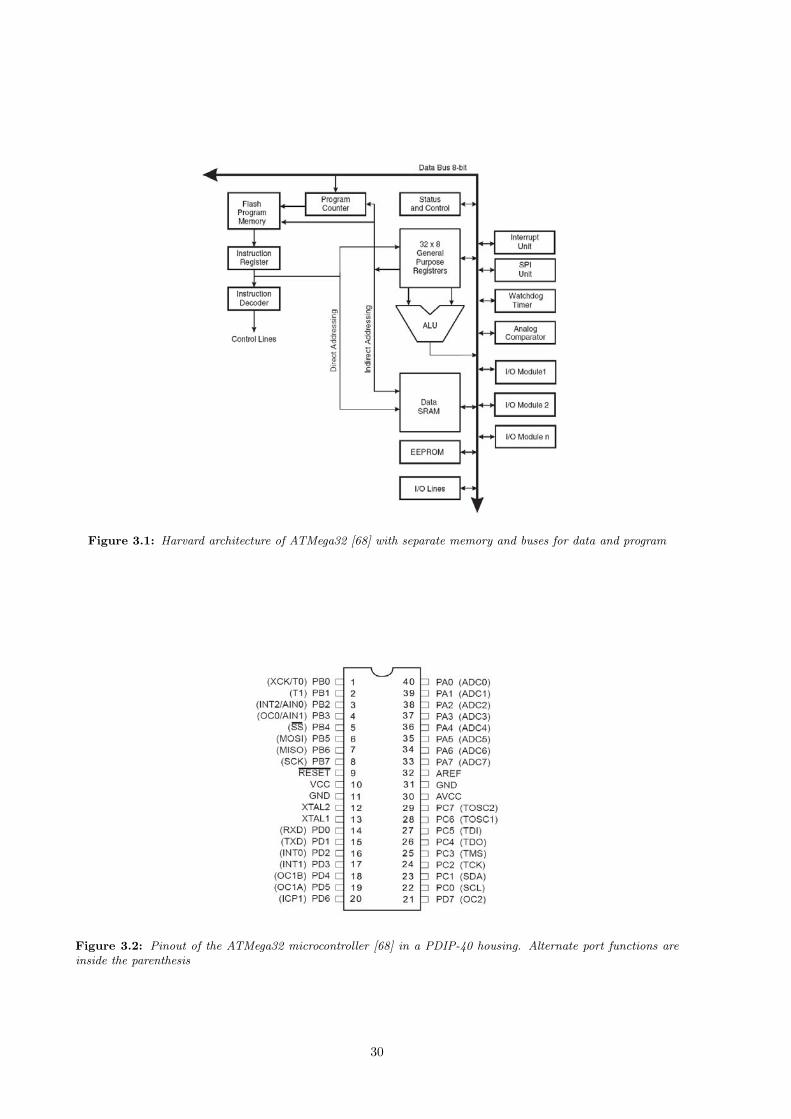
Figure 3.1: Harvard architecture of ATMega32 [68] with separate memory and buses for data and program

Figure 3.2: Pinout of the ATMega32 microcontroller [68] in a PDIP-40 housing. Alternate port functions areinside the parenthesis

30

3.1.3 Interrupts

Different asynchronous events may occur during the execution of a microprogram. Interrupts are usedto prevent the programmer from having to poll different status registers constantly, waiting for events tohappen. An interrupt can for example be caused by a level change on an external interrupt port, a counteroverflow or a complete reception of a serial data byte. The first 40 bytes of the program memory contains20 interrupt vectors. For each vector a jump command tells the microcontroller where in the programcode the triggered interrupt is to be handled. If a microprogram runs when an interrupt is triggered, theexecution of the program is halted. Then the interrupt is handled according to the interrupt vector. Thehandling should of course not take too long, or else the occurrence of other interrupts may be overseen.When the handling of the interrupt is done, execution of the main program continues from where it washalted.

3.1.4 Counters and Pulse Width Modulation (PWM)

Two 8bit counters and one 16bit counter are available on the microcontroller. In general, these consistof a counter register, a prescaler, control register and compare registers. The prescaler divides the globalclock signal of the microcontroller with either 1, 8, 64, 256 or 1024, allowing different counter speeds.The counters can be set to operate in three different modes. In normal mode, the counter starts countingfrom 0 and counts upwards until the counter register overflows (8bit/16bit). The overflow will trigger aninterrupt if the corresponding bit is set in the Timer/Counter Interrupt Mask Register (TIMSK) of themicrocontroller.

The second mode is called Clear Timer on Compare Match (CTC) and does, as the name suggests, areset of the counter when a compare value is reached. As the counter is reset, an interrupt is triggered ifset up in the TIMSK-register. An output pin on the microcontroller can be set to toggle on each comparematch, creating a clock signal with programmable frequency. By correct setup of the CTC-mode, aninterrupt can be triggered on a regular basis and thus update for example a clock register. The frequencyof the counter (FCTC) is written as function of the system clock (FCPU ), the prescaler (N) and the resetcompare value (OCR):

FCTC =FCPU

N · (1 +OCR)

The third mode of the counter is the Pulse Width Modulation (PWM). This mode can again havethree different modes of operation, called Fast PWM, Phase correct PWM and Phase and Frequencycorrect PWM. This section describes the Fast PWM mode.

Fundamentally, the PWM mode works a lot like the CTC-mode. First, a reset value is set for thecounter, deciding the frequency of the generated PWM-signal. In addition an output compare value is set.When the counter counts from 0 to the reset value, it compares its value with the output compare value.Depending on an inverting or non-inverting mode of operation, the output pin of the microcontrollercorresponding to the counter is toggled from 1 to 0 or from 0 to 1 when the counter value matches theoutput compare value. In this way, by choosing an output compare value between 0 and the reset valueof the counter, the duty cycle of the PWM-signal is controlled. The frequency of the Fast PWM signal iswritten as function of the system clock (FCPU ), the prescaler (N) and the reset compare value (OCR):

FFastPWM =FCPU

N · (1 +OCR)

Figure 3.3 illustrates the operation of the Fast PWM mode, where TCNTn is the counter register,OCRnx/TOP is the reset compare value, and OCnx is the output pin for the PWM signal. OCnx andOCnx represent respectively inverting and non-inverting mode of operation.

3.1.5 Universal Synchronous and Asynchronous Serial Receiver and Trans-mitter (USART)

For serial communication with its surroundings, the ATMega32 contains an USART. This function unitcan be set up to send and/or receive data on the TX and RX pins of the microcontroller allowing itto communicate with other microcontrollers, serial analog to digital converters, computers (with levelshifter like the MAX232 from maxim), GPS modules or any other device with an USART interface. The

31

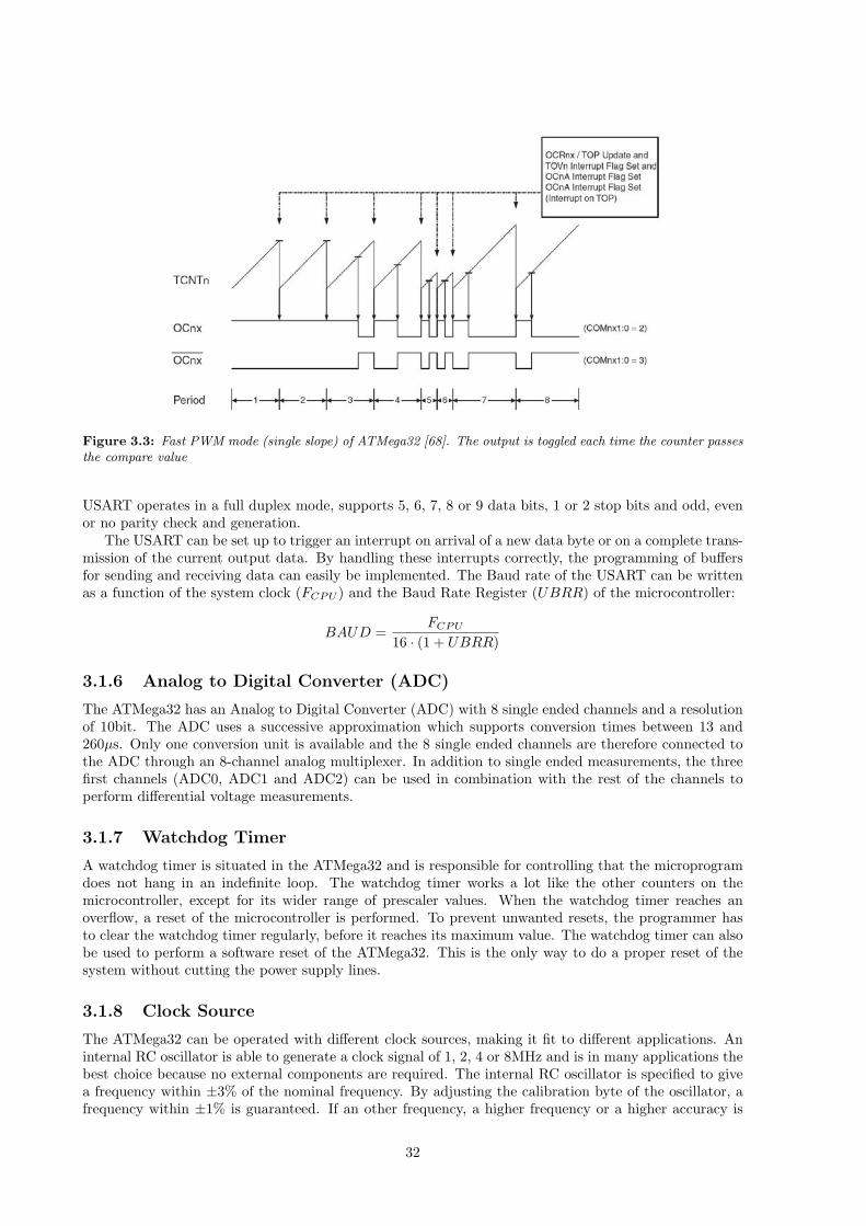
Figure 3.3: Fast PWM mode (single slope) of ATMega32 [68]. The output is toggled each time the counter passesthe compare value

USART operates in a full duplex mode, supports 5, 6, 7, 8 or 9 data bits, 1 or 2 stop bits and odd, evenor no parity check and generation.

The USART can be set up to trigger an interrupt on arrival of a new data byte or on a complete trans-mission of the current output data. By handling these interrupts correctly, the programming of buffersfor sending and receiving data can easily be implemented. The Baud rate of the USART can be writtenas a function of the system clock (FCPU ) and the Baud Rate Register (UBRR) of the microcontroller:

BAUD =FCPU

16 · (1 + UBRR)

3.1.6 Analog to Digital Converter (ADC)

The ATMega32 has an Analog to Digital Converter (ADC) with 8 single ended channels and a resolutionof 10bit. The ADC uses a successive approximation which supports conversion times between 13 and260µs. Only one conversion unit is available and the 8 single ended channels are therefore connected tothe ADC through an 8-channel analog multiplexer. In addition to single ended measurements, the threefirst channels (ADC0, ADC1 and ADC2) can be used in combination with the rest of the channels toperform differential voltage measurements.

3.1.7 Watchdog Timer

A watchdog timer is situated in the ATMega32 and is responsible for controlling that the microprogramdoes not hang in an indefinite loop. The watchdog timer works a lot like the other counters on themicrocontroller, except for its wider range of prescaler values. When the watchdog timer reaches anoverflow, a reset of the microcontroller is performed. To prevent unwanted resets, the programmer hasto clear the watchdog timer regularly, before it reaches its maximum value. The watchdog timer can alsobe used to perform a software reset of the ATMega32. This is the only way to do a proper reset of thesystem without cutting the power supply lines.

3.1.8 Clock Source

The ATMega32 can be operated with different clock sources, making it fit to different applications. Aninternal RC oscillator is able to generate a clock signal of 1, 2, 4 or 8MHz and is in many applications thebest choice because no external components are required. The internal RC oscillator is specified to givea frequency within ±3% of the nominal frequency. By adjusting the calibration byte of the oscillator, afrequency within ±1% is guaranteed. If an other frequency, a higher frequency or a higher accuracy is

32

needed, an external RC oscillator or an external crystal may be used. This may be the case in timingcritical applications. The last clock source option of the microcontroller is the operation with an externalclock signal. This option could for example be used in a system with a global clock signal and multiplesynchronous microcontrollers.

3.2 Keithley KUSB-3100

Figure 3.4: The Keithley KUSB-3100 has 12bit resolution and 50kS/s sample rate

The Keithley KUSB-3100 (figure 3.4) is a data acquisition (DAQ) unit with an USB interface. Italso comes with an application programming interface (API) for the Microsoft .NET Framework. TheDAQ unit has an internal 500V isolator barrier which protects the computer from external electricaldisturbance. Table 3.1 shows the technical specifications of the unit. The KUSB-3100 is divided intoseveral subsystems responsible for handling analog to digital conversion, digital to analog conversion,digital input, digital output and timer operation. These subsystems are exposed through the API.

Property ValueResolution 12BitThroughput 50kS/sAnalog input channels 8 Single endedAnalog output channels 2Digital I/O channels 16Counters/timers 1Gain 1, 2, 4, 8Connectivity Built in screw terminals

Table 3.1: Specifications of Keithley KUSB-3100 [69]

3.3 Microsoft Robotics Studio

In robotic applications, dealing with I/O is a very natural operation. This is the interface betweenthe robot and the real world. As robotic systems become more advanced, multi-threaded software isa natural leap towards imitation of the parallel processing capabilities of the human brain. However,the concurrency that multi-threaded systems possess also introduces some difficulties. Traditional I/Osystems normally have one connection to a control unit and multiple I/O channels. How would this be

33

handled in a concurrent system if one I/O channel is used to control a leg and another used to controla hand? If the concurrent system has one thread for computation of leg movement and one for handmovement, there is a possibility that these two threads will try to access the single hardware connectionsimultaneously.

In a normal application, such settings will have to be avoided using software programming techniquesfor multi-threading such as semaphores. This functionality is an integrated part of Robotics Studio whichaims to handle such settings hidden from the programmer of the leg and hand movement. This presumesthat the hardware process has been designed to handle concurrent requests properly. The following listsummarizes how Robotic Studio solves the challenge of I/O concurrency.

Hardware is abstracted and wrapped in a Robotics Studio Service

The hardware service can be reached from any other service

The hardware can be polled via messages to the hardware service

– The message handler decides if concurrent message handling is allowed

– Robotics Studio queues requests if no concurrency is allowed

Result

– The degree of allowed hardware concurrency is defined when writing the hardware service

– User does not need to worry about concurrent hardware request when writing services thataccess the hardware service

3.3.1 Overview

Microsoft Robotics Studio is a free framework for robotic application on the Windows platform and wasreleased in December 2006. The idea behind Robotics Studio is to create an environment of concurrentlyworking services which communicate with each other through different types of messages. There aretwo types of messages that can be sent between services. The first type is service operations, which arerequests for a certain action to be performed. Such an action can for example be a request to returnthe current state of the service, a request to return a HTML-representation of the state, a request toacquire data from hardware or simply a request to update values in the state of the service. This way ofsystem design, with independent modules, is also known as loosely coupled. The second message type isnotifications, which are sent from a service when a predefined event occurs.

3.3.2 Concurrency and Coordination Runtime (CCR)

The CCR is a programming model for Robotics Studio and can be said to be an abstraction from thedetails considering multi threaded computation like semaphores, locks and critical sections. Behindthe scenes, it handles all the work that normally would be done by hand in a system of concurrentlyworking modules. Therefore, a service developer doesn’t have to worry about the execution order of othercooperating services. The CCR itself is a dynamic linked library (dll) for .NET framework v2.0 or later,which means it is available through all languages targeting the .NET Runtime.

3.3.3 Decentralized Software Services (DSS)

The DSS is built on top of the CCR and is an application model which builds on the REST model.The principal of its operation is that a service is exposed to its environment by providing a state object.Expansion of the REST model includes structured data manipulation, event notification and servicecomposition. DSS is built to support applications which are sewn together from multiple services, whichcan run on different computers and communicate over a network.

The main component of DSS is services. A service can be seen as an object instance in traditionalobject oriented programming. Figure 3.5 shows a graphical representation of a service component. Theservice identifier is a unique URI address for the service, which all other services use to communicate withit. The service is assigned this address when it is constructed. The service contract is a short descriptionof the behaviour of the service which enables the composition or reuse of a service with a given contract.

34

Figure 3.5: DSS service model [70]. All communication with the service is done via its main port and notificationport

The service state is representing the current state of the service. It can for example contain thelatest acquisition data from a hardware module, the settings for a robot test drive or any other storedinformation. The state can be seen as the public domain of a service, defining what information thatcan be retrieved and what information that can be modified. The service partner list contains all theother services that the service is cooperating with through messages. In order to be able to talk to otherservices, they are required to be defined in the service partners list.

The main port of the service is a FIFO data structure, which handles all received messages from otherservices. Each service defines what type of messages it can handle on its main port, which forwards themessage to its corresponding service handler. The service handler handles the message and returns aconfirmation or, in the case of a data request, the requested data.

3.3.4 Visual Programming Language (VPL)

In contrast to conventional textual programming of DSS-services, Microsoft Robotics Studio also offersthe ability to do graphical programming with the Visual Programming Language (VPL). VPL is on onehand meant for beginners, with lack of experience in textual programming. On the other hand, it canalso be used by experienced programmers to prototype, to define services and for code generation. VPLprogramming is a description of the dataflow between services or service internal actions like calculations,variable assignments or other functions. In Figure 3.6, one can see how data values, variables andcalculations are used to construct a dataflow which finally is sent to a text-to-speech service. This simpleprogram first initializes a variable called Test with the value 1. The value is then sent to the text-to-speech service, which tells the user the actual value. A boolean comparison is then done between Testand the value 10. If Test is unequal to 10, it is incremented by 1 and then sent to the speech serviceagain. This is repeated until the value of Test is 10 and then the text string “All done!” is sent to thespeech service before the program is terminated.

Figure 3.6: Microsoft Visual Programming Language (VPL) [70]. A tool for beginners and for rapid prototyping

35

36

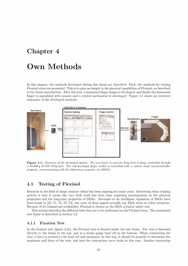
Chapter 4

Own Methods

In this chapter, the methods developed during this thesis are described. First, the methods for testingFlexinol wires are presented. This is to gain an insight in the physical capabilities of Flexinol, as describedin the thesis introduction. After this test, a humanoid finger design is developed, and finally the humanoidfinger is assembled with sensors and a control mechanism is developed. Figure 4.1 shows an overviewschematic of the developed methods.

Figure 4.1: Overview of the developed system. The test frame is used for long term testing, controlled througha Keithley KUSB DAQ-unit. The self-developed finger model is controlled with a custom made microcontrollerprogram, communicating with the laboratory computer via RS232.

4.1 Testing of Flexinol

Research in the field of shape memory alloys has been ongoing for many years. Interesting when readingarticles is that it seems like very little work has been done regarding investigations on the physicalproperties and the long-time properties of SMAs. Attempts to do intelligent regulation of SMAs havebeen found in [22, 71, 72, 73, 74], but none of these papers actually use SMA wires as robot actuators.Because of its commercial availability, Flexinol is chosen as the SMA actuator under test.

This section describes the different tests that are to be performed on the Flexinol wires. The mentionedtest frame is described in section 4.2.

4.1.1 Fixation Test

In the fixation test (figure 4.2a), the Flexinol wire is fixated inside the test frame. The wire is fasteneddirectly to the frame in the top, and in a strain gauge load cell in the bottom. When contracting thewire, a force is exerted to the load cell and measured. In this way, it should be possible to determine themaximum pull force of the wire, and how the contraction curve looks in this case. Another interesting

37

property to investigate is how the contraction changes over time. To be able to use Flexinol or similarproducts in real life applications, enough knowledge should be available to perform a proper scaling ofthe wires that act as a part of a bigger system.

4.1.2 Degeneration Test

This setup is designed to examine if a Flexinol wire suffers from degeneration when actuated continuouslyover time. One setup will be done with a small load (figure 4.2b), and a second setup (figure 4.2c) willbe done with a load, slightly smaller than the maximal pull force of Flexinol [37]. The parameter to beexamined is the strain rate of the wire, which optimally should not change too much. A wire that changesits working characteristics over time would in many applications lead to the need for a replacement ofthe wire. This complicates both the application design and the service routines. In the article Low-massmuscle actuators using electroactive polymers (EAP) [60], the author contends that shape memory alloyshave a life limit of 1000 cycles when actuated to maximal displacement. This should also be investigated.

The contraction rate is measured with two displacement transducers, located underneath the smallload and the big load as seen in figure 4.2b and 4.2c.

(a) Fixation.Can Flexinolstand this test,and how largeforces will beexerted?

(b) Long termtesting with asmall load applied

(c) Long termtesting witha heavy loadapplied

Figure 4.2: Test designs for Flexinol

4.1.3 Flexinol Antagonist

In this test, two Flexinol wires act together as antagonistic muscles (figure 4.3a). When one wire isfully contracted (agonist), power is cut and cooling of the wire begins. Simultaneously, the second wire(antagonist) contracts, causing a stretching of the first wire. By measuring the displacement and actuationforce over time, it can be examined if such an antagonistic use of two Flexinol wires causes degeneration.With this setup it should also be investigated at what maximal frequency the antagonistic muscles canbe actuated.

The contraction rate of the degeneration tests is measured with normal linear displacement transduc-ers. When testing antagonists, the center point of the generated motion is located in the middle of theframe and is not easily measured with a linear displacement transducer. Instead, a radial displacementtransducer is fastened on the top of the frame. A thread is fastened in the connection point of the twoFlexinol wires, pulled over the radial displacement transducer and then fastened in a nut, working as adead weight to keep the thread straight.

38

A strain gauge load cell is used to measure the force of each contraction. The forces exerted to thewires when one wire is turned off and the other on, are interesting because they show in what degree theopposite forces of the wires are able to overload eachother.

4.1.4 Spring Antagonist

This test (figure 4.3b) is similar to the test in section 4.1.3, except for the nature of the antagonist. Aspring is used as a passive antagonist instead of the active Flexinol antagonist in section 4.1.3. The testframe holds 100cm of Flexinol wire and with 4.5% strain rate, the spring antagonist will be stretchedabout 4.5cm. It has to be taken into concern, that a certain force is needed to stretch the wire, andtherefore the spring should be preloaded. A preloading of the spring will of course be a force workingagainst the wire, but this is the only way to utilize the maximum strain rate of the wire.

The deflection and forces caused by the wire is measured in the same way as for the Flexinol antagonist,described above.

(a) Flexinol wireperforming an ac-tive antagonisticmovement

(b) Spring per-forming passiveantagonisticmovement

Figure 4.3: Antagonistic test designs for Flexinol

4.1.5 PWM-controlled

As described in section 5.2, the results from the above mentioned tests revealed that the use of anantagonistic Flexinol wire is possible but complicated. The PWM-controlled setup therefore uses aspring antagonist, as described above. When controlling a finger, it is desirable to be able to control eachjoint to any degree of flexion. To be able to do this, the Flexinol wire has to be contracted to differentpoints between no contraction and full contraction. With most actuators this is an easy task, but as thedegree of contraction for a Flexinol wire depends solely on the wire temperature and the stress of thewire, this is a non-trivial task.

Some sort of regulation has to be used in order to control the wire. For the ease of design, theregulation loop should have as few sensor inputs as possible. For a regulation of the wire contraction,two variants will therefore be tested. The first variant uses sensor input from a deflection transducer tocontrol the wire contraction to a predefined set value. The second variant uses current measurements tocontrol the contraction. This variant may be difficult to get working, as the PWM-control signal alsocauses the current to be pulse width modulated.

With these two tests, it will become clear if it is possible to control the wires as wanted. If themethods are successful, they will also be used to control the humanoid finger.

39

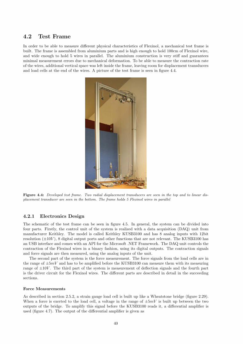
4.2 Test Frame

In order to be able to measure different physical characteristics of Flexinol, a mechanical test frame isbuilt. The frame is assembled from aluminium parts and is high enough to hold 100cm of Flexinol wire,and wide enough to hold 5 wires in parallel. The aluminium construction is very stiff and guaranteesminimal measurement errors due to mechanical deformation. To be able to measure the contraction rateof the wires, additional vertical space was left inside the frame, leaving room for displacement transducersand load cells at the end of the wires. A picture of the test frame is seen in figure 4.4.

Figure 4.4: Developed test frame. Two radial displacement transducers are seen in the top and to linear dis-placement transducer are seen in the bottom. The frame holds 5 Flexinol wires in parallel

4.2.1 Electronics Design

The schematic of the test frame can be seen in figure 4.5. In general, the system can be divided intofour parts. Firstly, the control unit of the system is realized with a data acquisition (DAQ) unit frommanufacturer Keithley. The model is called Keithley KUSB3100 and has 8 analog inputs with 12bitresolution (±10V ), 8 digital output ports and other functions that are not relevant. The KUSB3100 hasan USB interface and comes with an API for the Microsoft .NET Framework. The DAQ unit controls thecontraction of the Flexinol wires in a binary fashion, using its digital outputs. The contraction signalsand force signals are then measured, using the analog inputs of the unit.

The second part of the system is the force measurement. The force signals from the load cells are inthe range of ±5mV and has to be amplified before the KUSB3100 can measure them with its measuringrange of ±10V . The third part of the system is measurement of deflection signals and the fourth partis the driver circuit for the Flexinol wires. The different parts are described in detail in the succeedingsections.

Force Measurements

As described in section 2.5.2, a strain gauge load cell is built up like a Wheatstone bridge (figure 2.29).When a force is exerted to the load cell, a voltage in the range of ±5mV is built up between the twooutputs of the bridge. To amplify this signal before the KUSB3100 reads it, a differential amplifier isused (figure 4.7). The output of the differential amplifier is given as

40

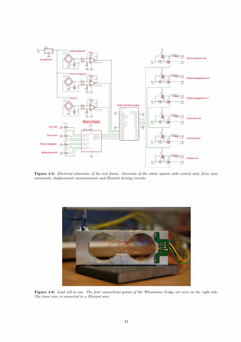
Figure 4.5: Electrical schematic of the test frame. Overview of the whole system with control unit, force mea-surements, displacement measurements and Flexinol driving circuits

Figure 4.6: Load cell in use. The four connections points of the Wheatstone bridge are seen on the right side.The loose wire is connected to a Flexinol wire

41

Vout =R2R1· (Vin+ − Vin−)

in the special case when R1 = R3 and R2 = R4. The load cells in use (figure 4.6) are rather cheap unitsthat are specified to about 200N. The load cells are not specified with a given mV/V, but the maximaloutput will be found when calibrating it. By measuring the mV output of the Wheatstone bridge andexpecting a maximum force of 30N, the gain factor is chosen to be ca 6800. This is done by settingR1 = R3 = 120Ω and R2 = R4 = 820kΩ. An excitation voltage of 5V is regulated by a MAX603 fromMAXIM, supplying the Wheatstone bridge. An 8V power supply is used for the operational amplifier.The choice of an 8V supply for the operational amplifier is to make the maximum output signal use alarge as possible part of the input range of the KUSB3100. The operational amplifier is an OPA2134from Burr Brown and was chosen because of its low offset.

Figure 4.7: Force signal amplification circuit with potentiometer used for balancing of the load cell

Measurement of the load cells when unloaded revealed that these suffer from an offset. This resultsin an bridge output of as much as 5mV when no load is applied to the load cell. The offset is amplifiedby the differential amplifier, which in the case of a 5mV input creates a theoretical output of ca 34V,which can not be output because the supply voltage of the op-amp is lower. To cancel the offset, thepotentiometer R5 is added to the circuit. R5 has a resistance of 0 − 1MΩ and is connected in parallelwith one of the resistors in the Wheatstone bridge. The chosen resistor should be on the side of the bridgewith the highest potential. By adding a potentiometer in parallel, the chosen resistor can be lowered,thus adjusting the output of the bridge. With a potentiometer with a maximum resistance of 1MΩ,the resulting resistance can be adjusted from near the value of the bridge resistor down to 0Ω and thus,balancing the bridge.

Displacement Signals

For the measurement of linear displacement, a linear variable differential transformer (LVDT) transducercan be considered. LVDTs operate with magnetic fields and can be produced to slide with almost nofriction. However, they need alternating currents (AC) to operate, which complicates the design. A setof resistive displacement transducers with removable return springs is used instead and are depicted infigure 4.8a. These work as a voltage dividers, making them perfect for applications using mainly directcurrent (DC). However, some friction might occur while sliding the stem through the housing. The maingoal of measuring forces in this setup is to see how the forces change over time, not to make a perfectabsolute force measurement. The forces exerted by the displacement transducers are therefore consideredto be small enough to be neglected.

For the two antagonist tests, the use of linear displacement transducers is a bit problematic. Asmentioned above, two radial displacement transducers are used instead. These are connected in the exactsame way as the linear transducers, like voltage dividers and are depicted in figure 4.8b. All displacementsignals are connected through a monitor for resistive displacement transducers (figure 4.10). The monitorhas four inputs and internally generates the excitation voltage needed. It has the ability to generate anexcitation voltage of 2.5V, 5V or 10V, and in this case 10V is used to take advantage of the whole inputrange of the KUSB3100 DAQ-board. The monitor also has the ability to correct for offset, but this isbetter done in software to prevent unwanted adjustments.

42

(a) Two displacement trans-ducers. To the left, the smallload can be seen. In the top ofthe image, the connection pointto a Flexinol is visible

(b) Radial displacement transducer. A thread is routed over to wheel tomeasure displacements

Figure 4.8: Displacement transducers

Flexinol Driver Circuit

The last part of the system schematic for the test frame is the driver circuit for the Flexinol wires. Thecircuit is depicted in figure 4.11 and only has one input through the small signal nMOS transistor T1(BSS98 [75]). The BSS98 has a maximum gate threshold voltage (VGS(th)) of 1.6V and should thereforeeasily be driven by the 5V digital outputs of the KUSB3100. The drain-source breakdown voltage is at50V which is more than enough to control the 15V that are used for the Flexinol wire. The drain pin ofT1 is connected to the gate of T2, a pMOS hexfet power transistor (IRF9540N [76]), able to control acontinuous drain current of 23A. This amount of current will require a heat sink when the transistor isoperated, but to control a 100cm of Flexinol wire (ca 15Ω), a current of ca 1A can be expected and thusshould the transistor not need a heat sink. The gate of T2 is driven actively low by T1 and pulled upby R16 when undriven. The Flexinol wire is connected to the drain of T2, illustrated as a resistor in theschematic.

4.2.2 Calibration

To ensure correct measurements, the displacement and force setups must be calibrated.

Displacement Calibration

The output from the displacement transducers are assumed to be highly linear, but nevertheless, acalibration routine is used to ensure this. A ruler is used to measure the amount of displacement whilethe corresponding output voltage is noted. This is done at eleven evenly distributed points between 0mmand 50mm of displacement. The generated table can then be plotted and the linearity can be controlledagainst a straight line. If the output proves to be linear, a linear gain factor should be calculated, orelse it must be decided what polynom degree to use. However, before calculating polynoms, it should beconsidered whether a non-linearity will cause problems or not in an overall view of the system. For theradial transducers, calibration is done between 0mm and 100mm.

Force Calibration

Strain gauge load cells will react to both positive and negative forces, and the easiest way of calibrationwhen the gauges are situated inside the frame would be to position different weights directly on top of

43

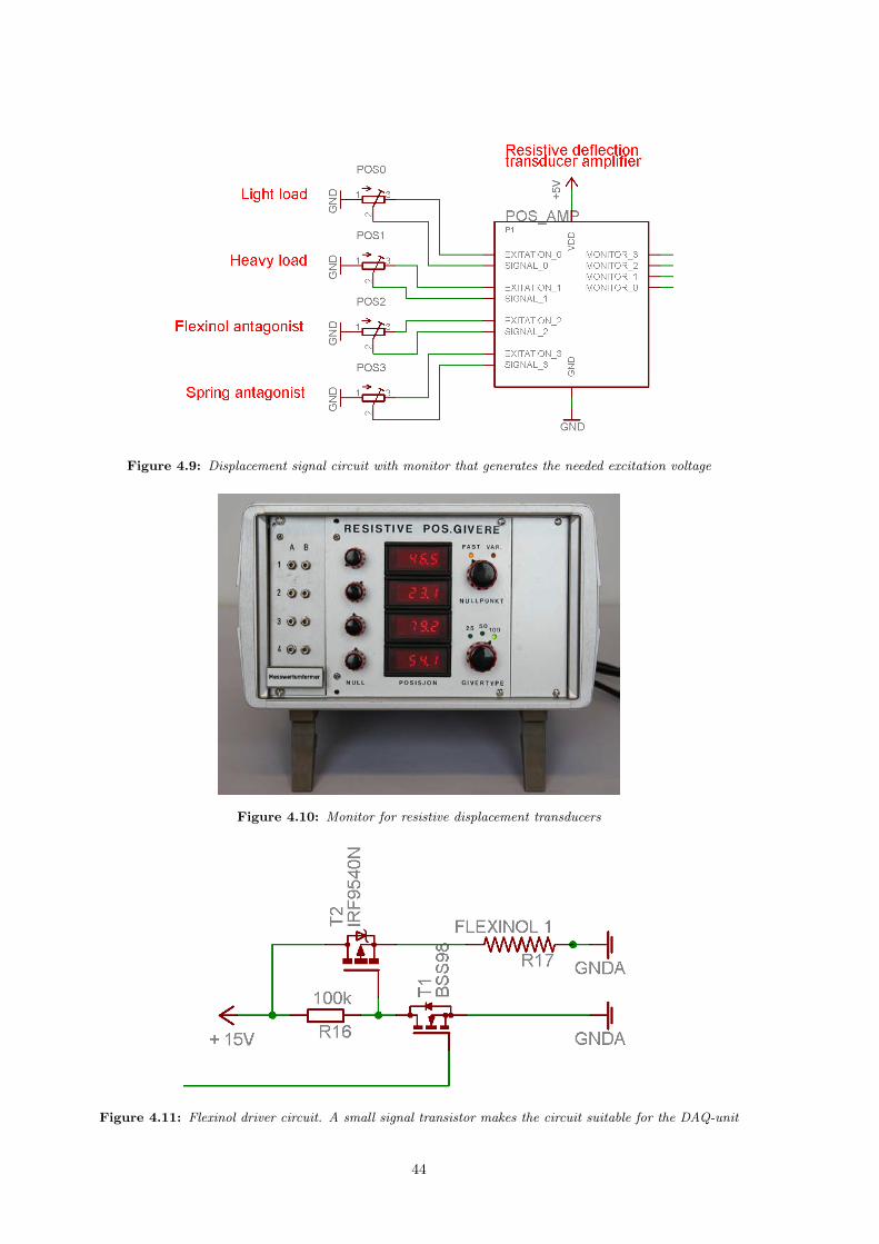
Figure 4.9: Displacement signal circuit with monitor that generates the needed excitation voltage

Figure 4.10: Monitor for resistive displacement transducers

Figure 4.11: Flexinol driver circuit. A small signal transistor makes the circuit suitable for the DAQ-unit

44

Calibrationforce

Calibrationweight

Strain gauge

Pulley frictionforce

Figure 4.12: Calibration setup for force measurements. The pulley introduces a small error in the force mea-surements

the load cells. However, the output may not be exactly proportional when calibrating this way. Instead,the wheel of a radial displacement transducer is used as a pulley. A thread is fastened in the load cell,pulling in upward direction. The thread is then pulled over the wheel as depicted in figure 4.12. This wayof calibrating will contain some error caused by friction when rolling the wheel of the radial displacementtransducer as illustrated in the figure. However, this error is considered small enough to be neglected.As already mentioned above, the main goal of the force measurements is to uncover relative changes overtime. To investigate the linearity of the load cells, calibration weights between 100g and 1500g with 100gsteps are used (figure 4.13). Analogous to the displacement calibration, a linear gain factor is calculatedif possible.

Figure 4.13: Calibration weights. Combinations of the weights are used to calibrate at 100g steps

4.3 Test Software

For the purpose of testing Flexinol wires, two programs are developed, one for controlling the test frameand one web application for remote surveillance.

45

4.3.1 Software for the Test Frame

For signal control, data collection and graphical presentation, a measurement program is written. Theprogram is developed in Microsoft Visual Studio 2008 and is written in the programming language C#for the Microsoft .Net Framework Runtime. A screenshot of the user interface can be seen in figure 4.14.The user interface consists of a set of tables continuously showing the last values for input and output,while the graphs show the same information graphically over time. The program has a simple menuwhere the measurements can be started and stopped, and while the program is running, a new setupfor output values can be loaded (described later). Figure 4.15 shows a block diagram of the programarchitecture. Each block is described in the next sections.

Figure 4.14: User interface of measurement software. Measurement values are seen in the top, plots in thebottom of the screen

Data Acquisition (DAQ) Module

The data acquisition module is responsible for communication with the KUSB3100 USB-device [69,77]. The device is divided into so called subsystems, one for each integrated function. In this module,analog inputs and digital outputs are handled. Therefore, the two subsystems AnalogInputSubsystem andDigitalOutputSystem are used. The digital output system is used at its simplest form by outputting onebyte of data. The 8 bits in the byte represent the digital state of the output channels. The control of thedigital outputs is described in the next section.

The analog signals from the test frame may contain some noise from the surroundings - mechanicalvibrations as well as electrical noise. To prevent this from influencing the measurement results, a simplemean filtering is used. When measuring analog values, the KUSB3100 can be used in either single modeor continuous mode. In continuous mode, the AnalogInputSubsystem is first configured with a conversionfrequency, a channel list and a data buffer. The conversion frequency is the raw frequency of the digitalto analog converter. If the subsystem is configured with a frequency of 1000Hz, a channel list with one

46

Figure 4.15: Block diagram of the program architecture. DAQ module communicates with the hardware and themain program handles inputs from the GUI

channel and a buffer for 1000 samples, the resulting buffer will contain 1000 samples of the specifiedchannel with 1ms delay between samples. However, if two channels are specified and the same frequencyand buffer is used, the resulting buffer will contain 500 samples of each channel with 2ms delay betweensamples.

When the DAQ-module receives an analog measurement request, the subsystem is configured with asuitable frequency, channel list and buffer. After the measurement is started, the module waits until thebuffer is filled, and then the mean value of the samples is calculated and returned.

Output Program Module

The program is supposed to control the Flexinol wires mounted in the test frame continuously for severalweeks. It must be expected that during this period, single wires will have to be replaced. It may also benecessary to change the output signal before mounting a new wire. To be able to perform this on the fly,without stopping the program, an output program module is developed. The output program tells theDAQ-module what control signals to output to the different Flexinol wires at all times. Each output hasits own array in the program module. Each time the DAQ-module sends a request to the output programmodule, the next value in the array is returned. The module can be replaced at runtime through the userinterface.

1 [ d o u t t i c k ]=10002 [ w i r e 0 ]=10* f a l s e ; 5* t rue ;20* f a l s e3 [ w i r e 1 ]=15* f a l s e ; 5* t rue ;15* f a l s e

The code above shows an example of an output program for two wires. The first line tells the DAQ-module how often it should request a new output value, in this case 1000ms. Wire 0 will in this case havea low output for 10 · 1000ms = 10s, then a high output for 5 · 1000ms = 5s and finally a low output for20 seconds. Because the driving of each Flexinol wire requires about 1A of current, it will be desirableto not have all wires contract at the same time. The output waveform of wire 1 from the above codewill be exactly equal to that of wire 0, with a delay of 5 seconds. When wire 0 turns off, wire 1 turnson, resulting in a 10 second period of 1A current instead of 5 seconds with 2A current. With only 2A ofcurrent flowing this will normally not be a problem, but with five wires driven at the same time, a currentof 5A would be expected. 5A is the upper limit for continuous current from the laboratory power supplyin use. When operated continuously for a longer period of time, this could cause problems because oftemperature variations in the surroundings.

Setup Module

To be able to change parameters for the program such as gain factors, mapping of outputs etc. withouthaving to change the program code, a setup module is developed. The setup module opens a text file

47

with lines formatted as

1 [ key ]= value

and stores these key-value pairs in a hash table. By providing the name of the key and the dataformat, the value corresponding to the key is returned. A global setup file is loaded on program startup,containing names of the five wires, corresponding output and input channels and gain factors. The outputprogram module mentioned above also uses the setup module to read the file containing the output values.

Graphical User Interface

The graphical user interface (GUI) was briefly presented above and is depicted in figure 4.14. The plot-ting of the signal data is done with the free scientific charting library NPlot (www.nplot.com). NPlotis a large library which supports many different types of plots, but is unfortunately not so well docu-mented. A few tutorials are available from the website, but the class descriptions are very short andlack examples. However, compared to other free plotting libraries like Chart FX Lite (www.softwarefx.com/SFXNETProducts/CFXLiteforNet) which contain limitations like maximum one data series, NPlotis considered to be a very good free solution. A small wrapper class is developed to hold track of thedata series to be plotted with NPlot. The wrapper class has a list of Y-data for all data series and a listof timestamps for the X-values. Each time the wrapper class gets new data, it deletes all data that isolder than the amount of seconds specified in the setup file. Then the new dataset is passed to NPlotand displayed. In this way, a charting functionality is created.

4.3.2 Web Application for Remote Surveillance

As mentioned above, the testing of Flexinol wires has a duration of many weeks and during this time,broken wires and other challenges are expected to occur. In order to remotely monitor the testing, a webapplication is developed. The main menu of the web application can be seen in figure 4.16 and consistsof a webcam picture, links to data from the five different wires and a survey of all wires.

The webcam picture is captured by the open source webcam capture program Dorgem, which isavailable from http://dorgem.sourceforge.net. It has a built in webserver listening on a selectableport, in this case port 8080. The webpage itself only contains an image reference to the url http://localhost:8080 and each call to this address causes Dorgem to return the latest captured image.

Each of the data links in the main menu lead to a list of available measurement data from thecorresponding wire, as seen in figure 4.17a. A new data file is created every day, and each file is availablethrough a link to a page that displays detailed information from the file. This page can be seen in figure4.17b and shows a couple of controls at the top and a plot of the selected data. Alternatively, the dataused to create the plot can also be displayed underneath it. The main goal of the web application is to beable to browse the measurement data, going back to see for example when a wire snapped. By using thecontrols at the top, a section of the file can be extracted and displayed. The first line of controls enablesthe user to choose any part of the file to display, alternatively only show every nth line of the selectedsection. The second line of controls makes it possible to display the n last lines of the data file.

Because special user rights are desirable, the computer used for measurements is not a part of thewired network at the University of Oslo (UiO). It therefore doesn’t possess a static IP address and instead,the address http://flexinoltesting.dyndns.org was assigned to the computer through the dynamicDNS provider www.dyndns.org. This makes the webserver easy to reach from inside the UiO network orvia VPN.

4.4 Humanoid Finger Design

This section focuses on the design of a humanoid finger, actuated with Flexinol wire. The design isinfluenced by some principles from the human anatomy, but is also an attempt to create a finger that canbe actuated with Flexinol wires without making the design too complex. The thoughts of how too designthe finger is highly influenced by the results from the testing of Flexinol (section 5.2) that revealed somelimitations and challenges. All presented 3D models are developed in the CAD software SolidWorks.

48

Figure 4.16: Menu for web surveillance. Web camera picture is updated each time the page is loaded

(a) Listing of available data.Filename, file size and the lastmodification date are shownin the listing

(b) Presentation of one single data file from the listing. By using thecontrols on the top of the page, different parts of the data file can beinspected

Figure 4.17: Data view from web surveillance

49

4.4.1 Anatomical Model

The presented finger is partially built up like the human finger. Mechanically, it consists of four phalangesconnected with three hinge joints. The joint between the metacarpal phalanx and the proximal phalanxis able to perform adduction and abduction by humans in addition to flexion and extension. Adductionand abduction is not a part of this mechanical design to keep it as simple as possible. If a good controllingof flexion and extension is achieved, this should be easily adaptable to adduction and abduction in laterdesigns.

As presented in section 2.1, the human anatomy uses muscles to create motions and tendons to transferthe motions. Tendon routing is done highly sophisticated in the human hand, causing for example thata flexion of the DIP-joint will automatically result in a flexion of the PIP-joint. This design makes thehuman hand highly suitable to grasp around objects. A good control of the contraction of the Flexinolwires would make such a design possible, but if not, it could make the finger impossible to control. Thisfunction of the human finger was therefore not used.

The extension of the finger is done in the same way as in the human hand. A single extensor tendonis straightening the joints on the upper side of the finger. The size of the finger segments are based onmeasurements of the hand of a 24 year old male.

4.4.2 3D Design

The 3D design is an attempt to combine the anatomical aspects from the last section with the abilitiesand limitations of the 3D printer Dimension SST 768. Figure 4.18 shows the end result of the designedparts. As the figure shows, most edges in the design have been rounded. This is done because straightedges tend to be rather weak when printed in ABS-plastic. Each finger segment has a height and a widthof 4cm and a varying length. As mentioned above, the finger sizes are based on measurements of a humanhand. To make a mechanical analysis easier, the finger is designed in a ratio of 3:1 to the measures. Theoversized design also makes more space available for tendon routing.

Figure 4.18: 3D design of a humanoid finger. The finger is designed in SolidWorks and then printed in ABSplastic

Metacarpal Phalanx (MCP)

The metacarpal bone of the human hand is inside the palm and therefore doesn’t appear as a part ofthe finger. In this design the metacarpal bone is used as a base for the hole finger construction and isdepicted in figure 4.19. On the back end of the finger segment, four holes can be seen in the top viewof the drawing. These are for mounting the finger and are positioned in the back to prevent obstructionof the finger movement. The joint at the other end of the segment is the first finger joint, namely themetacarpal phalangeal joint (MCP-joint). As can be seen from the top and bottom view in the drawing,

50

two slots are cut in from the end of the finger segment. These two slots will be connected with the nextfinger segment as described later. The radial part of the joint can be seen in the side view and ensuresthat the joint will be able to move freely over 90. As described later, the corresponding end of theconnected joint is also designed to fit exactly with the shape of the metacarpal phalanx, ensuring exactly90 of movement.

Bottom viewSide view Top view

Pivot point for MCP-joint

Screw holes

Channel forextensor tendon

Channel for allflexor tendons

Mounting holes

extensor tendonChannel for

flexor tendonsChannel for all

Channel for currentflexor tendon

Channel forcurrent flexor tendon

SolidWorks Educational LicenseInstructional Use OnlyFigure 4.19: Drawings of the metacarpal phalanx from different angles. This is the first finger segment and is

fastened to the forearm

As mentioned above, the human finger is designed in such a way that if the DIP-joint of the fingeris flexed, this will also cause a flexion in the PIP-joint. To prevent this kind of movement in the 3Dmodel, the tendons will be routed through the pivot point of each joint. When for example the end joint(DIP-joint) of the finger is flexed, the corresponding tendon will be tightened, exerting forces on eachjoint it is routed through. By routing the tendon as near as possible to the pivot point of the other joints,the exerted forces will be minimal, causing movement only in the correct joint. To make room for sucha construction, the center of each joint has to be kept free. As can be seen in the lowest part of figure4.19, this is done by splitting the joint axle in two parts, each one entering from its own side of the joint.The two axles are normal M5 screws with a length of 16mm. The outer screw holes have a diameter of5mm, allowing the screws to slide in without much friction. The inner holes have a diameter of 4.8mm,which is small enough to fasten the screws.

Figure 4.20: Tendon routing inside the finger. The tendon is routed through the pivot point of the joints, creatingminimal torque

51

Figure 4.20 shows the routing schematic for the hole finger. The routing channels can also be seenfrom different angles in figure 4.19. The channel for the current MCP-joint starts at the back end of theMCP, where all three flexor tendons enter the construction. Two tendons (green and blue) are routedstraight through the segment, through the pivot point and into the next finger segment. The currenttendon (red) is routed diagonally to the bottom of the finger segment and then along to the next segmentwhere it is connected. If a pulling force is exerted to this tendon, the result will be that the connectionpoint of the tendon on the proximal phalanx will be pulled against the MCP causing the joint to flex.

At the top of the routing schematic, a channel for the extensor tendon can be seen. This is just onesingle tendon that is routed through all the segments of the finger and connected with the last one. Toprevent damage to the extensor tendon, too much friction forces and unwanted forces when a joint isflexed, this channel is cut to align concentrically to the pivot point of each joint.

Proximal Phalanx

The proximal phalanx (figure 4.21) is the first finger segment with a joint in each end. The MCP-jointonly consists of two plates, fitting exactly into the slots of the MCP. A 5mm hole through the pivot pointof the joint allows the screws mentioned in the last section to be inserted. The other end of the proximalphalanx is the PIP-joint and is built up with two slots, exactly like the MCP-joint of the MCP segment.As figure 4.20 shows, the first flexor tendon (red) is connected to the lower side of the proximal phalanx.This is done by making a horizontal channel for the tendon as figure 4.20 and 4.21 show. A vertical holewith a diameter of 2.8mm is then cut through the tendon channel. This will allow a 3mm screw to bemounted into the hole, locking the tendon in place.

End (MCP)

Exit point for tendon channel

Extensor tendon channel

Bottom

Bottom viewTop view

Projections

Pivot point for PIP-joint

Side view

Tendon routing channels

Fastening point for tendon

Pivot point for MCP-joint

End (PIP)

SolidWorks Educational LicenseInstructional Use Only

Figure 4.21: Drawings of the proximal phalanx from different angles. This is the second finger segment

The proximal phalanx is a bit shorter than the metacarpal phalanx. As figure 4.21 and 4.20 show, thisresults in a shorter and steeper routing channel for the current flexor tendon (green). To prevent cornersin the routing channel, the channel is designed to be orthogonal to the pivot point of the MCP-joint. Inpractice, this means that the tendon will always go in a straight line from the pivot point to the lowerside of the proximal phalanx. The projection view of figure 4.21 clearly shows where the MCP flexor isconnected and where the PIP flexor exits. As with the metacarpal phalanx, the proximal phalanx alsohas a tendon channel for the extensor mechanism in the top of the construction.

52

Intermediate Phalanx

The intermediate phalanx is constructed very much like the proximal phalanx. The only difference isthat the intermediate phalanx is even shorter, making tendon routing a challenge. As figure 4.22 shows,the tendon channel is very steep, leaving almost no room for a tendon fastening mechanism. To be ableto fasten the tendon, a channel is constructed as for the proximal phalanx. However, this channel cannotbe cut in the longitudinal direction because it would then collide with the other tendon channel. Thefastening channel is therefore cut latitudinal, leaving enough room for both the fastening screw and thetendon channel.

As figure 4.20 shows, the tendon (blue) that is routed through the intermediate phalanx is the lastflexor tendon, responsible for flexing the DIP-joint. The extensor channel is routed through the top ofthe phalanx as for the two previous finger segments.

Bottom

End (DIP)

Exit point for flexor tendon channel

Extensor tendon channel

Projections

Bottom viewTop view

Pivot point of DIP-joint

Side view

Pivot point of PIP-joint

Fastening point for flexor tendon

End (PIP)

SolidWorks Educational LicenseInstructional Use Only

Figure 4.22: Drawings of the intermediate phalanx from different angles. This is the third finger segment

Distal Phalanx

The distal phalanx is the last finger segment and therefore differs from the others. Figure 4.23 showsdrawings of the distal phalanx. The PIP-joint of the segment is built up exactly as described for the otherfinger segments with two plates fitting into the other side of the joint. The other side of the phalanx isrounded, making it look like the finger tip of a human finger. Both on the upper and lower side of thefinger segment, fastening mechanisms for tendons are situated. The upper one is for the extensor tendon,and has its entering hole inside the PIP-joint. A screw hole is cut to fasten the tendon. Analogous to theproximal phalanx, a tendon channel is cut in the longitudinal direction, assuring a tight fastening of thetendon.

4.5 Humanoid Finger Application

As already mentioned, the above presented design is prototyped with a 3D printer. The resulting finger,produced in ABS plastic, now has to be assembled and put into a finger application. In general, the

53

Side view Top view Bottom view

Projections

Pivot point of DIP-joint Fingertip

Screw hole for extensortendon fastening

Fastening mechanism for flexor tendon

Channel for extensor fastening

SolidWorks Educational LicenseInstructional Use Only

Figure 4.23: Drawings of the distal phalanx from different angles. This is the tip of the finger

application consists of three main parts. The main mechanical part is the finger which is supplied withtendons in the form of the fishing line FireLine from Berkley (www.berkley-fishing.com). The finger isfastened to the second part of the application which is a rectangular aluminium tube, acting as a forearm,holding three Flexinol muscle fibers, an extensor return spring and sensors for displacement and force.Finally, an electrical circuit controlled by an Atmel ATMega32 is used to control the muscle fibers, readsensor data and communicate with a computer. Figure 4.24 shows a picture of the finger mounted onthe forearm.

4.5.1 Mechanical Design

The base of the mechanical design is a rectangular aluminium tube. The tube is used to wire sensorsand power supply, keeping them away from the hot Flexinol wires which potentially could melt the wireisolations, causing short circuits. The aluminium tube could have been used as electrical ground, but thiswas considered too hazardous. If a wire would break near to the end with the highest potential, and thebroken wire would touch the tube, large currents would be expected (1Ω⇒ 15A). This could potentiallyoverheat and damage some parts of the electronics.

Elastic Displacement Transducer

A first attempt to measure the displacement of the muscle fibers is done with an elastic displacementtransducer. The principle of this measurement is depicted in figure 4.25. The elastic transducer has aresistance that changes when the transducer is stretched. It is fastened to the joint between the tendonand the Flexinol wire in a stretched state. When the Flexinol wire is contracted, the joint moves to theright, shortening the transducer. By including the transducer in a voltage divider, a voltage proportionalto the amount of contraction can be measured. However, as the results in section 5.4.1 shows, themeasurements are not stable, making the transducer unsuitable for this application.

54

Figure 4.24: Assembled finger mounted on an aluminium forearm. The finger segments are connected withnormal machine screws

Finger

Tendon Flexinol wire

Elastic transducer

Joint

Block

Figure 4.25: The elastic displacement transducer (blue) changes its resistance when it is stretched

Radial Displacement Transducer

To overcome the problems of the elastic displacement transducer, a small radial transducer is developedinstead (figure 4.27). The transducer is based on a standard one turn trimmer potentiometer which iseasily soldered onto a PCB strip board with 2.54mm grid. A bracket is designed to fasten the strip boardin a upright position on the aluminium tube. A principle schematic can be seen in figure 4.26.

The expected displacement from the Flexinol wire is about 4.5cm, and to ensure that the transducercan handle this, a wheel with a diameter of 2cm is designed. This makes one turn on the potentiometerequal to a length of π · d = π ∗ 2cm = 6.28cm. A first version of the wheel is depicted in figure 4.28a.The tap in the center of the wheel is mounted inside the potentiometer and then fastened with a screw.The tap appeared to be the weakest structure of the printed part, so a second version of the wheel isdeveloped (figure 4.28b). Instead of the tap, a screw is fastened through the potentiometer, directly intothe wheel. A washer is used to separate the wheel from the body of the potentiometer.

The potentiometer is wired as a voltage divider, causing its output to span from 0V to Vdd. This leadsto a better resolution than the elastic transducer, that would need a resistor in series towards ground.The transducer wheel was developed in SolidWorks and printed on the 3D printer.

Bracket for Force Measurements

The strain gauges used for force measurements in the test frame are too large in size to be fitted intothe finger application. Instead, a pressure sensor is used (section 2.5.2). The sensor can be seen in figure4.29 and is mounted together with a bracket at the end of a Flexinol wire. The bracket is designed in3D and printed on the 3D printer. It consists of two base parts, each with a hole through the center to

55

Finger

Tendon Flexinol wireJoint

Block

Rubber band

Radial transducer

Figure 4.26: A thread is used to rotate the radial displacement transducer. The thread is returned by a rubberband

Figure 4.27: Radial displacement transducer mounted on the forearm. Rubber band and Flexinol wires can alsobe seen

(a) Version 1. The center tap proved tobe to weak when printed in ABS plastic

(b) Version 2. The wheel is held inplace by a screw instead of the tap

Figure 4.28: 3D model of radial displacement transducer wheel

56

fasten screws. The base also has one hole in each corner. Two of them are for fastening screws and twoof them can be used with a screwdriver in order to fasten screws in the other base part. The bracket alsohas two washers between the bases. One of them has a slot where the pressure sensor can be inserted.The pressure sensor is then held in place after the screws have been mounted. The last washer is pressedagainst the pressure sensor when the base parts are forced away from each other and thus, making a forcemeasurement possible.

(a) Version 1. The circular design leftlittle room for mounting screws.

(b) Version 2. The rounded rect-angle shape allows mounting ofscrews in the corners.

(c) Printed bracket is fixated in oneend. When the Flexinol wire is tight-ened (lower part of image), a force canbe measured.

Figure 4.29: 3D model of force bracket

Force Calibration

The pressure sensor changes its resistance when a weight is pressed against it. To calibrate the pressuresensor, the force bracket is mounted inside the above mentioned test frame. A hook is fastened to thelower end of the bracket, allowing different weights to be hung on it. By applying weights in the spanfrom 100g to 1500g with steps of 100g a good calibration curve is achieved.

4.5.2 Electrical Schematics

Figure 4.30 shows the electrical schematic drawing for the finger application. The control unit of thesystem is represented by an ATMega32 microcontroller. The microcontroller controls the Flexinol wiresthat are driven with the same circuit as depicted earlier in figure 4.11. A 5V voltage regulator suppliesthe microcontroller and is used as excitation for displacement and force measurements. A 6 pin ISPconnector is used as programming interface for a computer running the development tool AVR Studiofrom manufacturer Atmel.

4.5.3 Communication

The finger application is designed to be a remotely controlled stand-alone system. As can be seen fromthe schematics in figure 4.30, a MAX202 driver chip is connected to the ATMega32. The MAX202 isneeded to convert the 0V-5V TTL signal levels from the microcontroller to RS232 levels of ±12V . Thedriver (figure 4.31) uses its 5V supply voltage together with a charge pump to build up +12V over anexternal capacitor. This voltage is then inverted with another charge pump to provide −12V . The TX-and RX-pins of the ATMega32 are connected to T1in and R1out, correspondingly.

57

Figure 4.30: Electrical schematic for the finger application. The ATMega32 microcontroller is used for mea-surements, computations and output signals

The MAX202 is connected to a DB9 connector with a minimal connection (ground, rx and tx), whichis sufficient for this application. A computer can then be used to connect to the finger application viaRS232.

Figure 4.31: Maxim MAX202 level shifter for serial communication between ATMega32 microcontroller andhost computer[78]

4.5.4 Microcontroller Program

The ATMega32 is controlling the Flexinol wires and reading sensor inputs. For these tasks, a micro-program is needed. Programs for the ATMega32 are normally written in C and compiled with the freeWinAVR compiler. Some prefer to write programs directly in AVR assembly, but this solution shouldonly be chosen if the programmer needs control over every clock cycle, as assembly has a much lowerreadability and scalability than the C language. A block diagram of the program can be seen in fig-ure 4.32. A command interpreter is developed to provide a flexible remote interface. The implementedinterpreter is presented in the following section.

58

Figure 4.32: Block diagram of the micro program. Reception of commands is done by the UART module, analyzedby the interpreter module and executed in the main program

Command Reception

As already mentioned, the program receives commands over the UART interface. The reception of datacan occur occasionally and should therefore be handled in a suitable way. There are in general two waysto check whether a data byte has been received. The first method is to check the status register of theUART regularly. This method applies large limitations to the program, as the UART has to be polledcontinuously to avoid losing data bytes. Instead, the reception of data is done with interrupts. A bufferis implemented as an array, capable of holding 50 bytes of data. The interrupt service routine puts thereceived data byte in the first free position of the buffer each time an interrupt is triggered. At the sametime, the interrupt service routine checks if the received data byte is a newline character. If this is thecase, a complete command has been received and has to be analysed.

Command Analysis

The analysis of a command is performed by the interpreter. The interpreter consists of two main functions.The first function is used to determine which command is present. This is done by comparing thefirst characters of the received buffer to the different commands supported by the interpreter. Thecomparison function in use is called strncasecmp(S1,S2,len) and is available in the string.h of the WinAVRdistribution. The second function of the interpreter is a method to extract the arguments of the command.This function takes two arguments - a reference to the buffer and the number of arguments to look for.It loops through the buffer and converts every ASCII represented argument to a binary format. Thefunction stops when it finds a newline character, but before it returns, it checks if enough arguments havebeen found. It then returns a 0 if enough arguments are provided, 1 if not. By allowing commands to besent in a ASCII format, more buffer memory and more processing power is needed. However, this ensuresa command interface that is easier to use and to debug than an interface dealing solely with binary data.

Command Execution

When the interpreter has found a matching command and the number of arguments is found to becorrect, a corresponding command flag is set in the main program loop. The main loop holds one flag foreach operation it supports and the only task of the loop is to check whether one of these flags has beenset. If this is the case, the corresponding function is executed. This behaviour means that during theexecution of an operation, the command interface will react to new commands and set command flags,but the arguments of a new command will overwrite the last arguments. To prevent such an unwantedbehaviour, a busy flag is introduced. This flag is set to 1 during an operation, and by sending thecommand BUSY? over the interface, the current state is returned.

59

Command Set

Command Arguments DescriptionIDN? 0 Returns an identifier string for the programPWM? 1 Returns the current PWM duty cyclePWM 2 Sets the current PWM duty cycleCURRENT? 1 Returns the result of a current measurementDEFLECTION? 1 Returns the result of a deflection measurementFORCE? 1 Returns the result of a force measurementCONT CURRENT DEFLECTION 7 Starts a continuous measurement of current

and deflectionCONT CURRENT 4 Starts a continuous measurement of currentCAL CURRENT 1 Calibration function for current controlCONT DEFLECTION 4 Starts a continuous measurement of deflectionCAL DEFLECTION 1 Calibration function for deflection measure-

mentsCONT FORCE 4 Starts a continuous measurement of forceSET DEFLECTIONS 6 Sets the amount of wanted deflection in all

jointsSET DEFLECTION 4 Sets the amount of wanted deflection in one

jointSET CURRENT 4 Sets the amount of deflection controlled by the

measured currentSET FORCE 4 Sets the amount of deflection controlled by the

measured forceBUSY? 0 Returns the current state of the programSTOP 0 Stops the current operationRESET 0 Causes a watchdog reset to be performed

Table 4.1: Command set for the microcontroller program

Table 4.1 shows all the operations that the interpreter is programmed to receive. The IDN? commandis just an identification command supported by many instruments. A string containing the name of themicro program and the version number is returned. The control of the three Flexinol wires is done witha PWM-signal. The duty cycle of these signals can be set using the command PWM ch value, where chis the channel number (0-3) and value is the duty cycle (0-255). The actual PWM signal for the channelch can be queried in the same way with the command PWM? ch.

1 // Set duty c y c l e o f PWM channel 0 to 50\%2 PWM 0 1283

4 // Read the cur rent duty c y c l e o f PWM channel 15 PWM? 1

The function DEFLECTION? ch causes the ADC unit to perform a measurement of the specified Flexinolwire. The result of the measurement is the mean value of five measurements with 1ms delay betweeneach. The mean value is then converted from ADC units to volts and returned with three decimals ofprecision. The FORCE? ch command works in the same way as DEFLECTION?, returning the mean valueof five measurements of the specified force channel.

1 // Read d e f l e c t i o n from channel 02 DEFLECTION? 03

4 // Read f o r c e from channel 25 FORCE? 2

60

To be able to visualize the data from the sensors, different continuous functions are developed.The command CONT CURRENT DEFLECTION cch0 cch1 cch2 dch0 dch1 dch2 delay performs continu-ous measurements of each of the current channels (cch) and deflection channels (dch) marked with ’1’.The number of milliseconds of delay between each measurement is specified in the last argument. Foreach measurement, the mean value is sent over the RS232 interface to the host computer. The followingcode demonstrates how to setup the microprogram to perform 5 measurement per second of current anddeflection on channel 0.

1 // Read cur rent channel 0 and d e f l e c t i o n channel 0 every 200ms (5Hz)2 CONT CURRENT DEFLECTION 1 0 0 1 0 0 200

The results from such a measurement can hopefully be used to make a regulation algorithm thatcontrols the amount of deflection by controlling how much current is flowing through the Flexinolwire (temperature dependent, see section 2.3). Similar to CONT CURRENT DEFLECTION, the commandsCONT CURRENT, CONT DEFLECTION and CONT FORCE perform continuous measurements of current, deflec-tion and force respectively.

1 // Read cur rent channel 0 every 20ms (50Hz)2 CONT CURRENT 1 0 0 203

4 // Read d e f l e c t i o n channel 1 every 50ms (20Hz)5 CONT DEFLECTION 0 1 0 506

7 // Read f o r c e channel 2 as f a s t as p o s s i b l e8 CONT FORCE 0 0 1 0

The commands described so far does not include any form of regulation, they are solely meant toanalyse the behavior of Flexinol. There are in general three ways to regulate the contraction rate ofFlexinol in this application. The first and most direct way to regulate is to use the deflection measurementas feedback in the regulation loop. To use this method, the microprogram first has to be calibrated withthe outer boundaries of each finger joint. This is done with the command CAL DEFLECTION, which performsan automatic calibration. The program presumes that each finger joint is completely stretched when thecommand is executed. The calibration algorithm first reads the value from the deflection sensor and usesthis as the first boundary (0o). The Flexinol wire corresponding to the same joint is then turned on,making the joint flex. A delay of 1500ms is added to the algorithm in order to be sure that the wirestarts to contract. The deflection sensor is then read every 500ms and compared to the last read value.When the difference between the two values is less than 0.01V , the algorithm saves the last deflectionmeasurement as the second boundary (90o) and then turns the wire off. The procedure is then repeatedfor the two other joints.

When the calibration is done, the commands SET DEFLECTION or SET DEFLECTIONS can be used toregulate the Flexinol wires. SET DEFLECTION only regulates one wire and has the channel, the amount ofdeflection, regulation factor and verbose as parameters. It is only meant for testing purposes as normallyall three joints of the finger will be regulated. SET DEFLECTION uses the same regulation algorithm asSET DEFLECTIONS. SET DEFLECTIONS is the main regulation command in the application. It takes onedeflection value for each joint, a regulation factor, a verbose flag and how often a verbose should occuras arguments.

1 // Ca l i b ra t i ng d e f l e c t i o n2 CAL DEFLECTION3

4 // Regulate each j o i n t to 45 degrees , r e g u l a t i o n f a c t o r 10 ,5 // verbose every 100 th r e g u l a t i o n c y c l e6 SET DEFLECTIONS 128 128 128 10 1 100

The regulation algorithm first calculates the deflection sensor value corresponding to the set valuefrom the user. This is written as

sensorV alue = min+(max−min) · setV alue

255

61

where min is the deflection sensor value at 0o and max is the deflection at 90o. setV alue is the de-flection value provided through the command arguments. The algorithm then reads the actual deflectionD and calculates the absolute error value err

err = setV alue−D

Then the correction value errP is calculated as

errP =err · 255

max−min· reg

64The expression takes the relationship between the error err and the total span between min and max

and multiplies it with the regulation factor reg. If the regulation factor is chosen to be smaller than64, a dampening of the regulation is achieved. If it is chosen to be greater than 64, an amplification isachieved. The value of errP is then added to the current PWM output signal. After the new PWMvalue is calculated, the algorithm checks if the verbose flag is set and checks the verbose frequency valueto see if the current values should be sent via RS232. The values of the verbose flag decides what valuesare to be sent according to table 4.2.

Decimal Binary Description0 0b0000 No output1 0b0001 Only the current PWM value2 0b0010 Only the current deflection4 0b0100 Only the current force/current3 0b0011 Deflection and PWM value5 0b0101 Current/force and PWM value6 0b0110 Current/force and deflection7 0b0111 Current/force, deflection and PWM value

Table 4.2: Values for the verbose flag. By choosing the correct flag, a selection of what data to return from themicrocontroller can be done

The second regulation method uses the amount of current flowing through the wire to control theamount of deflection. As described in section 2.3, the electrical characteristics of Flexinol changes asa function of contraction. This means that by knowing how much current is flowing through the wireat different contraction rates, this can be used to control the wire to the same contraction rate using acurrent measurement as feedback. This solution has the advantage that it in general does not need adeflection sensor, desirable to minimize systems. However, the electrical characteristics also have a secondparameter, namely the amount of stress that is exerted to the Flexinol wire. In the scope of this thesis,regulation is done with only current as feedback, with no stress applied to the wires while regulating. Tocalibrate the algorithm, the command CAL CURRENT is implemented. CAL CURRENT is dependent on theCAL DEFLECTION command to be executed in advance. It divides the complete deflection range into 16equal steps and regulates to each of them with deflection as feedback. At each step, a mean value of 150current measurements is saved. The result of the calibration is an array holding 16 values describing howmuch current is excepted at different rates of contraction.

When the calibration is done, the command SET CURRENT is used to start the regulation. SET CURRENTtakes four arguments - the channel to regulate, the current step to regulate after (0− 15 = 0o− 90o), theregulation factor and a verbose flag. The current flowing through the Flexinol wire is determined by thePWM signal from the ATMega32. This means that the current flowing will have the same characteristicsas a PWM signal, alternating between no output and maximum output. To control the wires as accurateas possible, the mean value of the current should be measured. This is done by an external RC-filter.Unfortunately, the PWM signal has a rather low frequency, and the RC filter therefore has a time constantτ = RC that is rather high. This leads to an unwanted delay in the regulation loop. The regulation itselfuses the same proportional regulation as SET DEFLECTIONS.

1 // Ca l i b ra t i ng d e f l e c t i o n2 CAL DEFLECTION3

4 // Ca l i b ra t i ng cur rent s t ep s f o r wire 0

62

5 CAL CURRENT 06

7 // Regulate wire 0 to cur rent s tep 7 (45 degree s ) with r e g u l a t i o n8 // f a c t o r 100 and verbose f l a g s e t9 SET CURRENT 0 7 100 1

During a regulation or calibration, the micro program must be stoppable. This is implemented witha stop flag, similar to the start flags described above. The command BUSY? may first be used to checkwhether the micro program is currently running any functions. If this is the case, the command STOP maybe sent to abort the current operation. All functions that do regulation and calibration are programmedto set all PWM outputs to 0 when the STOP command is received. For unwanted program states duringdevelopment, the command RESET is implemented. RESET enables the watchdog timer and sets its timeout value to 15ms. It then waits in an infinite loop until the watchdog resets the microcontroller. In thisway, a software reset can be done that in normal cases is guaranteed to cause the same effect as powercycling does.

4.5.5 Computer Interface Program

The regulation algorithms and calibration routines described so far are all implemented in the microcon-troller. However, the need for sensor data analysis and a command interface makes an interface programnecessary. The program supports different profiles, making it backwards compatible with older versionsof the microcontroller program. At program startup, the user has to choose which profile folder is tobe used. The folder contains one file with all commands and one file with all commands that causes aregulation loop to be executed.

Command Mode

Figure 4.33 shows the first mode of the program, the command mode. In this mode, the user chooses oneof the commands in the list on the left side of the screen. The available commands, argument names andstandard values are read from the command file described above. When the user selects a command, thecorrect number of text boxes for arguments are shown with corresponding argument names and standardvalues. When the green send button is pressed, a text string is concatenated from the command and itsargument values. The string is then sent to the microcontroller via the serial port. At the same time thestring is written to the main text field and a timer is started in the background. The timer is set to checkthe RS232 receive buffer for new data. If the buffer contains a complete line terminated with a newlinecharacter, the line is printed to the main text field on the screen. The red stop button is programmed toquickly send the STOP command to the microcontroller in case of unwanted behaviour or emergencies.

Figure 4.33: Command mode of the interface program. This mode is used to execute single commands

63

ASCII mode

The second mode of the interface program can be seen in figure 4.34 and is called the ASCII mode. ASCIImode is the simplest form of communication with the microcontroller and is in reality only a terminalprogram. When the send button is pressed, the text in the input field is sent to the microcontroller andlogged in the large text field. A timer is then started analogous to the command mode. The ASCII modeis meant for command prototyping and easy debugging.

Figure 4.34: ASCII mode of the interface program. This mode is used to prototype and debug with text input

Continuous Mode

The third program mode is the continuous mode, depicted in figure 4.35. The continuous mode containsa list on the left side of the screen, similar to the command mode. The commands available are read fromthe file with continuous commands as described above. This mode is used to visualise the different sensorsignals over time. As the figure illustrates, instead of a text field, a plotting surface is available. TheY-axis of the graph is auto scaling. The length of the X-axis is adjustable during use to allow differenttime resolutions. The continuous mode also contains a checkbox that controls whether or not the receiveddata is to be saved. If yes, all data is saved to an auto generated file in the program folder.

4.5.6 Interface for Microsoft Robotics Studio

As described in section 3.3, the Microsoft Robotics Studio is a framework for robotic applications aimingto provide a fast and powerful base for development. A prototype service is therefore developed to connectthe finger with Robotics Studio. Figure 4.36 shows a screenshot of an interface that is integrated in theweb based control panel of Robotics Studio. The service communicates with the microcontroller via thesame module that was used in the interface program in section 4.5.5. The static nature of html pagesmakes interactive feedback of sensor data difficult, and therefore only a selection of the microcontrollerfunctions are realized. As depicted in the figure, the first table shows if the service is connected to themicrocontroller and provides buttons for connecting, resetting or stopping the current function runningon the microcontroller. The second table shows the last set of sensor readings. These values are updatedevery time the page is refreshed. Finally, the last table allows the user to set the duty cycle of eachPWM-output or to start the regulation of a given amount of flexion in the joints.

4.6 Summary of Own Methods

In this chapter, a number of self developed methods have been presented. Firstly, different mechanicaltests for the Flexinol muscle fibers were proposed. A test frame was built to perform the tests that

64

Figure 4.35: Continuous mode of the interface program. This mode is used to plot data from continuousmicrocontroller commands

were controlled and monitored by a self programmed measurement software, running on a laboratorycomputer. A web application was developed to be able to monitor the tests from a remote connection.

A 3D model of a humanoid finger was then developed using the CAD software SolidWorks. The modelwas produced in ABS-plastic with a 3D printer and then mounted to an aluminium tube. Tendons wererouted and connected to Flexinol wires for actuation. An electronic circuit was built, using a microcon-troller as control unit for the Flexinol wires and for sensory input. A microprogram was developed torun on the microcontroller, containing a command set with a number of different control options. Aninterface program was developed to interact with the microcontroller from the laboratory computer viaRS232. An optional interface for Microsoft Robotics Studio was also developed.

65

Figure 4.36: Web interface for the humanoid finger, implemented in Robotic Studio. The user can control thefinger through the control panel

66

Chapter 5

Experiments

This chapter describes the results from the methods presented in the previous chapter. First, calibrationresults for force and displacement are given. These results are necessary to perform measurements whiletesting Flexinol. Secondly, the results from the testing of Flexinol is given and finally, the developedhumanoid finger is discussed.

5.1 Calibration Results

Calibration of the test frame was done according to section 4.2.2. Although some non-linearities werediscovered, these were considered small enough to be negligible both for displacement and force. Bothcalibration result tables contain columns named NL (non-linearity). NL is the deviation from a straightline through the calibration points, calculated by the method of least squares. The calculated line iswritten as y = Ax+B, where A is the gain and B the offset found in the calibration tables.

5.1.1 Displacement Calibration

Table 5.1 shows the calibration results for the displacement transducers. The left part of the tablecontains values for the linear displacement transducers while the right part contains values for the radialtransducers. The negative values are caused by the displacement monitor that generates the neededexcitation voltage. The first radial transducer was calibrated with 0-90mm as the output value woulddrop before 100mm was reached.

The results from the calibration are visualized in figure 5.1. The calibration curves show that theoutput is near to linear. This assumption is also confirmed by the NL-columns of the table. All over,the NL varies around 0.03V for the linear displacement transducers, which equals about 0.34mm whenscaled. This is less than 1% of the 50mm measuring range. The worst case is an error of 0.076V , whichequals 0.8mm and 1.6%. For the radial transducers, the NL varies around 0.04V which equals about0.43mm, less than 0.5% of the 100mm measuring range. The worst case is an error of 0.073V , whichequals 0.8mm and 0.8%.

All mentioned error values are considered negligible.

5.1.2 Force Calibration

Table 5.2 shows the results from the force calibration. By looking at the calibration curves in figure 5.2and the NL-values in the table it becomes clear that the load cells are also linear. The highest error valueis 0.038V , which equals about 18g and 0.18N . This error is considered negligible.

5.2 Testing of Flexinol

The aluminium test frame described in the previous chapter was used to fasten and test Flexinol wiresin different setups. The frame was designed to hold 5 parallel wires of 1m in addition to displacementand force sensors. It proved to be large and stiff enough for all tests.

67

Small load Heavy Load Flexinol Ant. Spring Ant.cm ch 0 [V] NL ch 1 [V] NL cm ch 2 [V] NL ch 3 [V] NL0,0 -0,060 0,037 -0,103 0,076 0 0,277 -0,044 -0,105 0,0730,5 0,340 -0,025 0,239 -0,048 1 1,322 -0,007 0,783 0,0281,0 0,803 -0,023 0,717 -0,036 2 2,324 -0,013 1,641 -0,0481,5 1,300 0,012 1,222 0,003 3 3,370 0,025 2,585 -0,0382,0 1,750 0,000 1,688 0,003 4 4,415 0,062 3,546 -0,0102,5 2,217 0,006 2,154 0,003 5 5,376 0,015 4,488 -0,0023,0 2,670 -0,003 2,598 -0,019 6 6,383 0,014 5,361 -0,0623,5 3,117 -0,017 3,075 -0,009 7 7,373 -0,004 6,332 -0,0254,0 3,590 -0,006 3,555 0,005 8 8,380 -0,005 7,306 0,0164,5 4,057 0,000 4,008 -0,008 9 9,350 -0,043 8,253 0,0295,0 4,538 0,019 4,511 0,029 10 9,196 0,039

Offset 0,105 0,194 -0,318 0,192Gain 1,083 1,072 0,992 1,071

Table 5.1: Calibration table for displacement. The results show that the displacement transducers can be consid-ered linear

Figure 5.1: Calibration curve for displacement. Almost no non-linearities are visible. Small deviations are seenaround 0mm displacement

68

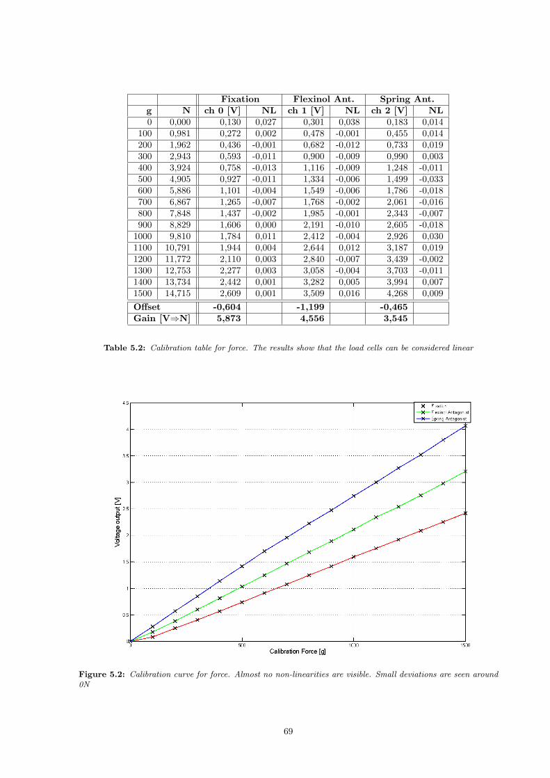
Fixation Flexinol Ant. Spring Ant.g N ch 0 [V] NL ch 1 [V] NL ch 2 [V] NL0 0,000 0,130 0,027 0,301 0,038 0,183 0,014

100 0,981 0,272 0,002 0,478 -0,001 0,455 0,014200 1,962 0,436 -0,001 0,682 -0,012 0,733 0,019300 2,943 0,593 -0,011 0,900 -0,009 0,990 0,003400 3,924 0,758 -0,013 1,116 -0,009 1,248 -0,011500 4,905 0,927 -0,011 1,334 -0,006 1,499 -0,033600 5,886 1,101 -0,004 1,549 -0,006 1,786 -0,018700 6,867 1,265 -0,007 1,768 -0,002 2,061 -0,016800 7,848 1,437 -0,002 1,985 -0,001 2,343 -0,007900 8,829 1,606 0,000 2,191 -0,010 2,605 -0,018

1000 9,810 1,784 0,011 2,412 -0,004 2,926 0,0301100 10,791 1,944 0,004 2,644 0,012 3,187 0,0191200 11,772 2,110 0,003 2,840 -0,007 3,439 -0,0021300 12,753 2,277 0,003 3,058 -0,004 3,703 -0,0111400 13,734 2,442 0,001 3,282 0,005 3,994 0,0071500 14,715 2,609 0,001 3,509 0,016 4,268 0,009Offset -0,604 -1,199 -0,465Gain [V⇒N] 5,873 4,556 3,545

Table 5.2: Calibration table for force. The results show that the load cells can be considered linear

Figure 5.2: Calibration curve for force. Almost no non-linearities are visible. Small deviations are seen around0N

69

5.2.1 Test Software

The main task of the test software is to perform measurements and to control output signals, as describedin section 4.3.1. During the first weeks of testing, the computer used for the measurements tended to runout of memory. A memory leak was suspected, and a first attempt to find the error was done with theMicrosoft CLR Profiler, a help tool to locate memory leaks. The profiler showed clearly that the memorywas growing constantly, which confirmed the assumption of a memory leak. As memory was growing withlittle steps, a new assumption was made that the leak had to be in either the function controlling theoutput or in the function performing the input measurements. The error was finally found to be in themeasurement function. Each time a measurement was started, the Keithley KUSB unit was configuredwith its setup. This function, provided by Keithley, has a minor memory leak that causes about 14KB ofmemory to be used every time the function is called. Over time this demands a great amount of virtualmemory, causing the computer to slow down. The problem was solved by reorganizing the code, makingthe configuration call only once.

Although the memory leak was fixed, the program seemed to slow down after a couple of days ofrunning. The amount of used memory was stable and the program used about 50% of the processorpower. The reduced speed of the program sometimes caused the output to be a little delayed or causedthe frequency of the input measurements to slow down. This again caused some of the measurement datato have a lower time resolution than wanted. However, the program speed was varying and not all cycleswere affected by the low measurement frequency. Therefore the problem was left unsolved, considered tobe a minor problem.

5.2.2 Fixation Test

The first setup described in the previous chapter is the fixation test (figure 4.2a). The wire was fastenedas described in section 4.1.1. In the top of the frame, a threaded stem was used to adjust the wire sothat it would be tight. The fixation test soon proved itself to be the most work demanding. Each wiremounted, tended to break after approximately two days of actuation. The wire break was always insidethe upper or lower fastening mechanism, suggesting that the method for fastening the wire is causingsome damage to it.

The first six wires that were tested were unfortunately tested with an erroneous amplifier setup. Twoerrors were found that certainly have caused wrong force measurements. The first error was the zeroadjustment of the strain gauge. The bridge had not been properly adjusted so that with no force applied,the output of the amplifier would be its lower rail. When applying a force, the output would remain atthe lower rail until the strain gauge had a large enough output signal to drive the amplifier above thelower rail. This caused an offset error, but also infected the calibration values that were calculated.

The second error that was found also concerned the amplifier. The maximum force measured from thewire with the erroneous setup was 30N. This is three times more than reported in the Flexinol datasheet[37] and therefore it did not appear as obvious that this value actually was the upper rail of the amplifier.However, as the first data analysis was done, it became apparent that the maximum value was the samefor every contraction cycle. The gain of the op-amp had been set too high and thus was the output rangeof the amplifier too small.

To correct the two errors, a zero adjustment was first done as described in section 4.2.1. Then asmaller gain was chosen before a new calibration was done. The new setup showed that the real pullforce of the wires was even larger than the first erroneous results. The maximum pull force that wasmeasured exceeded 40N, more than four times the reported maximum pull force. The pull force reportedin the datasheet of course refers to the recommended pull force.

Although the first six measurements had to be considered invalid in terms of determining pull forcedegeneration over time, they were not completely in vain. An important property was uncovered, namelythe lifetime of a wire when loaded to its maximum. The lifetime can be seen in table 5.3 and is givenas number of contraction cycles before the wire breaks. The column of maximal force contains erroneousresults for the first five wires caused by the wrong amplifier setup described above. The delay columnshows the time it takes after the wire is turned on until it reaches a force of 5N. The break point tellswhere the wire snapped.

70

Wire Cycles Max force [N] Delay [s] Break Point1 1969 31.05 1.2 bottom2 1501 31.06 0.9 top3 1504 31.04 1.4 top4 1193 31.05 1.2 bottom5 1971 31.06 1.1 top6 512 40.3 0.85 top7 7876 41.5 0.6 bottom

Table 5.3: Results from testing a fixated Flexinol wire. The wires always broke either in the upper or lowerfastening mechanism

Measurement Cycle

Figure 5.3 shows the measured force of a wire together with its control signal. A small time delay canbe observed between the rising edge of the control signal and the actual contraction start. As describedin section 2.3.2, this is caused by the warm-up time of the Flexinol wire. Analogous, a delay is seen asthe output is turned off, caused by the cooling time of the wire. As the wire reaches its maximum forceof around 40N, the force signal seems to become rather unstable. When the wire is in this state, thetemperature is much higher than normally needed to contract the wire. But because of the applied stress(fixed wire), the wire cannot contract. The temperature at this point is probably more than 100oC,making the difference between the wire temperature and its surrounding temperature very large. Anexplanation for the unstable behaviour could therefore be that the constantly cooling and heating of thewire at this point causes some kind of oscillation. It should be noted that four times the recommendedstress is applied to the Flexinol wire at this point.

Figure 5.3: Two contraction cycles of a fixated Flexinol wire. The maximum force of ca 40N shows that Flexinolis able to exert rather large forces

71

Degeneration

In figure 5.5, the degeneration of Flexinol over time is illustrated. The figure shows the actual pull forceof the wire through about 8000 cycles. Each graph value is the difference in force from the start of acontraction to the top of the contraction curve. As mentioned above, the signal is rather unstable whenthe wire is at its maximum force, this is also reflected by the rather large deviations in the curve. Fromcycle 1 to about 3100, a reduction in force is noticed. This was first assumed to be caused by a weakeningof the wire but turned out to be caused by a stretching of the wire. At cycle 3100, the wire was tightenedand as the graph shows, this causes an increase in force. The figure also shows a constant decrease in forceafter the tightening which also mainly is caused by a stretching of the wire. Surprisingly, the pull forceof the wire after tightening is almost as large as that of a new wire. The stretching of the wire continuesfor each cycle and it would be interesting to see if the stretching converges. During the performed tests,this was never observed as the wire would break before a trend could be seen. At around cycle 5800, anexternal disturbance caused a series of erroneous measurements that should not be evaluated.

Both between cycle 1 and 500 and between cycle 6000 and 7000 some additional noise can be seen onthe curve. This is most likely caused by temperature variations in the surrounding environment. Thesevariations can be caused by an open window, the central heating of the building or sunshine. However,regardless of the wire being stretched and an unstable test environment, the wire proves that its pullforce is very large until the point when the wire snaps. All the wires that were tested snapped at eitherof its ends. This indicates that the fastening mechanism of the wire is somehow causing damage to thewire, either at time of fastening, at time of contraction, or both. An attempt was made to improve thefastening mechanism. A thin copper plate was cut and placed inside the fastening mechanism betweenthe screws and the Flexinol wire. This did not seem to improve the lifetime of the wire, and the problemwas left unsolved as this only was occurring at this particular test setup with a load greatly exceedingthe recommended limitations of Flexinol. Overcoming this problem could maybe make it possible to testthe fixated wire over a longer period of time. This, however depends on whether or not the rest of thewire is close to snapping when the fastenings have snapped. Maybe a fastening of the wire with a knotsimilar to the clove hitch, seen in figure 5.4, can be used to prevent the fastening mechanism from beingthe weakest link. This, however would probably make the fastening mechanism both larger in size andmore complex.

Figure 5.4: A Clove Hitch knot could maybe be used to create a more gentle fastening mechanism for the Flexinolwires.

In figure 5.6, a detailed view of two contraction curves can be seen. The red curve shows a contractioncycle after 500 contractions and the blue curve shows contraction cycle after 4500 contractions. Onedifference that can be observed is a slightly lower pull force after 4500 cycles than after 500. This may becaused by a stretched wire, as described above. Some delay in the cooling of the wire can also be seen,but this is probably due to the time resolution of the measurement software because the slope of the twocooling curves are near to identical.

As already mentioned, a delay occurs between the rising edge of the output signal and the start ofthe contraction. Figure 5.7 shows the time between the rising edge of the output signal and the pointwhere the force signal is larger than 5N. This can be seen as the reaction time of the wire. The figureshows many high reaction times that are a result of the time resolution of the measurements. However,the interesting part of the data is that the reaction time from the correct measurements seem to be stablearound 0.5s− 0.8s over the whole period. This observation together with the observations around figure5.6 can therefore be used to conclude that only a small, negligible change is done to the transformationcurve of the wire during the test.

72

Figure 5.5: Degeneration of a fixated Flexinol wire over time. The decrease in force is caused by the wire beingstretched

Figure 5.6: Comparison between contraction curve after 500 and after 4500 cycles for a fixated Flexinol wire.Only very small differences are observed

73

Figure 5.7: reaction time of a fixated Flexinol wire. The curve shows the time from the wire is turned on untilthe measured force exceeds 5N. No changes can be observed over time

5.2.3 Degeneration Test

The two degeneration tests are described in section 4.1.2.

Small Load

In the first test, only a small load was supposed to be used to stretch the wire after a contraction. Thecontrol signal for the test is depicted in figure 5.8. First, a weight of 110g was molded in lead and fastenedto the wire. The result of this test clearly shows that the applied weight is to small to stretch the wire(figure 5.9). During the first hours of operation, the wire stretches less and less after each contraction,and after one day the Flexinol wire only has about 1.5mm difference between contracted and stretchedstate. Table 5.4 shows a survey of the performed tests. The most interesting result is from wire 4, where48861 cycles were completed. The initial deflection was 41mm and the ultimate deflection was 22.5mm.

Wire Cycles Max deflection [cm] Min deflection [cm]1 5866 2.9 02 7 - -3 1662 2.9 1.454 48861 4.1 2.25

Table 5.4: Results from testing a Flexinol wire with a small load. The fourth run is the first run with a largeenough weight. The very high number of contraction cycles should be noted

A number of washers were then fastened on top of the lead weight, making its total weight 200g. Thiswas not enough, so another 75g was added. With 275g, the wire could be stretched about 20mm butwas unstable from cycle to cycle. The wire was therefore replaced in case it had been damage throughbeing contracted for several days (figure 5.9). This seemed to be the case, because after changing wires,an improvement in stability could be seen. These results can be seen in figure 5.10, where the longduration of the test also should be noted. The gaps in the data is caused by computer breakdown and

74

power loss during the measurement period. Applying such a small load to the wire seems to cause verylittle damage to it. The difference between the contracted state and the stretched state of the wire isillustrated in figure 5.11 and it can be seen that in contraction cycle 1, the deflection is about 37mm.The degeneration of the wire is clearly visible between cycle 1 and cycle 15000 where it seems to convergetowards a deflection of about 22.5mm. This amount of deflection seems to be very stable as it is repeatedfor the next 30000 cycles.

It is very valuable to know that the wires converge towards a stable deflection rate after a while.However, with a stable contraction rate of about 22.5mm, only 2.25% deflection is achieved. This hasto be considered very low compared to the initial rate of 3.7% and the specified 4.5 − 5.0%. Anotheraspect of this test is the size of the applied weight. The maximum recommended pull force reported bythe manufacturer of Flexinol is 930g. When 275g are needed to stretch the wire, this equals about 1/3of the maximum, which has to be considered fairly high, limiting the working range.

Figure 5.8: Two contraction cycles for a small load. About 4% contraction is observed for the first two cycles

Heavy Load

The second of the two degeneration tests is similar to the first one, except for the weight being used tostretch the wire. Again, a weight was molded from lead and trimmed to be ca 930g, the same as therecommended maximum pull force of the Flexinol wire. The weight was fastened to the end of the wireand placed on top of a deflection transducer with a return spring. The return spring causes a small errorto the applied weight, but was considered to be negligible. Table 5.5 shows the results from all the testedwires. The life time of each wire varies very little. However, the average life time of ca 12000 cycles isabout 1/4 of the life time of the above mentioned wire with a small load.

The control signal for the test can be seen in figure 5.12 together with the deflection. By looking atthe time axis, it can be seen that the frequency of this test is the double of the frequency for the lightweight. This is due to the fact that the heavy weight stretches the wire much faster than the light weightdoes.

Results from one test can be seen in figure 5.13 and 5.14. As the figures show, a very stable deflectionof about 4.25mm is observed. However, as figure 5.13 shows, the wire is continuously stretched under

75

Figure 5.9: Deflection over time with 110g applied. 110g proved to be insufficient to stretch the Flexinol wireafter a contraction

Figure 5.10: Deflection over time with 275g applied. 275g was enough to stretch the Flexinol wire after acontraction and also proved not to overload it

76

Figure 5.11: Difference between contracted state and stretched state from figure 5.10. The contraction rateconverges towards 2.25% after 15000 contraction cycles

Wire Cycles Max deflection [cm] Min deflection [cm]1 11910 4.5 4.12 11399 4.4 4.33 12994 4.4 4.24 11531 4.25 4.05 12158 4.3 4.2

Table 5.5: Results from testing a Flexinol wire with a heavy load. Very similar results for all five runs can beobserved. The deflection rates of about 4.5% are equal to the information found in the Flexinol datasheet [37]

the load of the 950g. After about 3 days (5500 cycles) the wire was therefore tightened to keep it insidethe 50mm measuring range of the deflection transducer. Figure 5.14 shows that the deflection transduceralready was at its lower limit, causing a slight increase in deflection when tightening the wire. Afterabout 11000 cycles, the wire snapped without any warning signs in terms of radical changes in deflectionor speed (figure 5.15).

5.2.4 Flexinol Antagonist

The use of an extra antagonist wire to stretch an agonist wire is described in section 4.1.3. The firstattempt with this method can be seen in figure 5.16. As the graph shows, the agonist wire produces asmall force when actuating. This comes from stretching the cold antagonist wire. However, when theagonist wire is turned off and the antagonist wire is turned on, a large force is produced. This is becausethe agonist has not yet been cooled down while the antagonist starts to stretch it. As a result, both wiresare stretched. This can also be seen be looking at the figure. The figure shows the 8 first cycles of thetest, and during this short time the deflection is reduced from 15mm to 6mm. The maximum deflectioncould have been about 25mm as each wire has a length of 50cm. During the same period, the force isalmost halved, also reflecting that the wires have been deformed. A second attempt was therefore donewith a more conservative control signal. Two cycles from this attempt can be seen in figure 5.17. As the

77

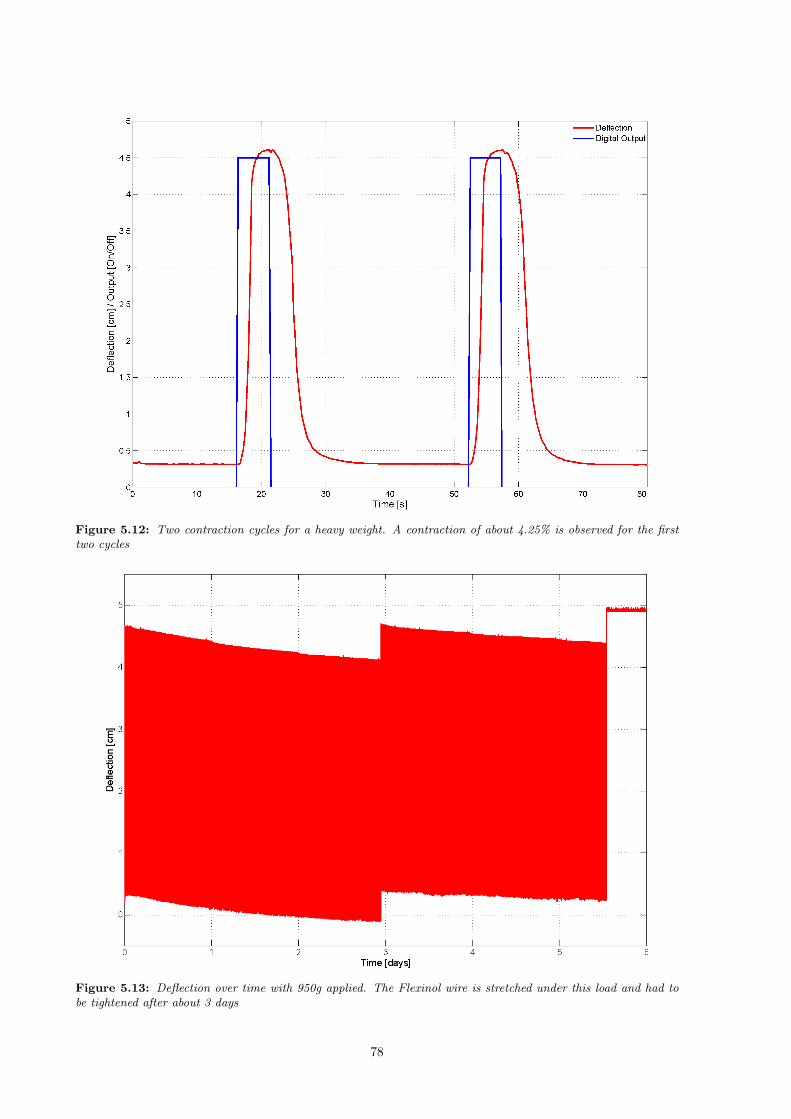
Figure 5.12: Two contraction cycles for a heavy weight. A contraction of about 4.25% is observed for the firsttwo cycles

Figure 5.13: Deflection over time with 950g applied. The Flexinol wire is stretched under this load and had tobe tightened after about 3 days

78

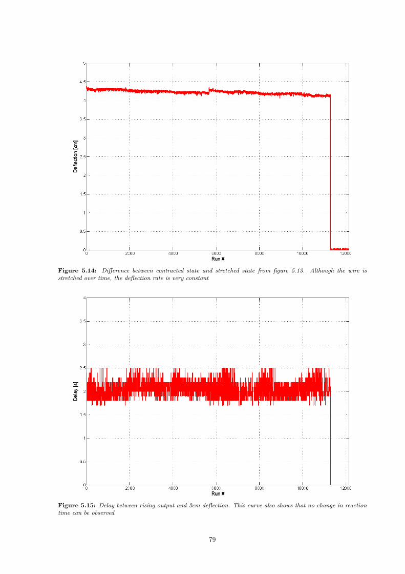
Figure 5.14: Difference between contracted state and stretched state from figure 5.13. Although the wire isstretched over time, the deflection rate is very constant

Figure 5.15: Delay between rising output and 3cm deflection. This curve also shows that no change in reactiontime can be observed

79

graph shows, much smaller forces are exerted compared to the first attempt, indicating a more gentle useof the wires. A deflection of 22mm is equivalent to 4.4%, which is a rather good utilization. However, asfigure 5.18 shows, the deflection decreases almost linearly towards 0mm during the first 500 contractioncycles. Although performing better than the first attempt, this indicates a rather strong deformation ofthe wires as a result of the antagonistic behaviour. After about 600 cycles the wires were tightened butthey were deformed rather fast, as the graph shows. At about 3900 cycles, a third attempt was doneto tighten the wires with the same result. Table 5.6 shows results from the tested wires. The two firstwires were unsuccessful setups and therefore, only the third wire shows useful numbers. The maximumdeflection is observed in the first contraction cycle, but as the table shows, after some time, the deflectionis down to 0mm. This is also reflected by the minimal and maximal forces.

Wire Cycles Maxdeflection

[cm]

Mindeflection

[cm]

Max force[N]

Min force[N]

1 5690 0.5 0 30 02 345 0.3 0 30 03 5182 2.1 0 15 0

Table 5.6: Results from testing a Flexinol antagonist. The mechanism suffers from unnecessary large forces thatstretches the wires and results in a malfunction

After these attempts the idea of using an active Flexinol antagonist was not further investigated.This was because of the time demanding and inconvenient assembly of the wires in addition to the ratherpoor performance described above. Maybe an even more conservative way of controlling the wires couldprevent the deformation of the wires. However, the contraction cycle described in figure 5.17 is alreadycontaining a delay of 10 seconds between agonist and antagonist. A longer delay would be even moreinconvenient if the Flexinol wires are used for example in a robot hand.

Figure 5.16: Eight contraction cycles for a Flexinol antagonist. Very large changes can be seen during the cycles

80

Figure 5.17: Two contraction cycles for a Flexinol antagonist. A more conservative timing diagram results inmore gentle control with smaller forces being exerted

Figure 5.18: Difference between contracted state and stretched state with Flexinol antagonist. The wires aredeformed very quickly, making the deflection converge to 0mm

81

5.2.5 Spring Antagonist

The use of a spring as antagonist is described in section 4.1.4. It differs from the use of a Flexinolantagonist in being a passive return force. Two contraction cycles for this test are shown in figure 5.19,where a force measurement can be observed in addition to the digital output signal and the deflectionsignal. The force measurement may seem redundant as it is proportional to the deflection because of thespring constant. However, it also tells the pretensioning of the spring. The pretensioning is importantas it decides the speed of the stretching, but also how much the wire is stressed. This again, also hasimpact on how much the wire is stretched. A large preload of the wire seems to shorten its lifetime butalso causes larger deflections. A smaller preload decreases the deflection slightly, but ensures a slightlylonger life of the wire.

Table 5.7 shows results from the tested wires. Wire 1 was tested with almost no pretensioning,reflected by the low deflection rate. Both for wire 2 and 3, the pretensioning was increased, resulting inincreased deflection in both cases, but also shorter lives of the wires.

Wire Cycles Max deflection [cm] Min deflection [cm]1 21497 3.0 2.12 20964 3.6 33 18836 3.8 3.3

Table 5.7: Results from testing Flexinol with a spring antagonist. Very stable results can be observed for the lifetime, but deflection rates are reduced when using a spring as antagonist

Figure 5.20 shows the development in deflection over time. The graph shows clearly that after a shortperiod of settling, only a very small degeneration of the wire occurs. Although the wire shown in thefigure snapped before a convergence was obvious, the trend of the deflection graph seems to be goingtowards a limit of about 32.5mm.

Figure 5.19: Two contraction cycles for spring antagonist. Very gentle control of the wire is achieved. The forcevalues also reflect this

82

Figure 5.20: Difference between contracted state and stretched state with spring antagonist. It is apparent thatonly a small degeneration is done to the wire during 20000 cycles

5.2.6 PWM-Control

The PWM-control is done with two types of feedback, deflection and current.

Deflection Controlled

The PWM-control of the Flexinol wires was first done with a displacement feedback in the regulation loop.The regulation was performed with the function SET DEFLECTIONS that is a part of the microcontrollercommand set, described in section 4.5.4. As described in section 4.1.5, the regulation is done on a singleFlexinol wire with a spring antagonist as return force.

The regulation was done with different regulation factors that are depicted in figure 5.21. The mostapparent observation from the results is the oscillation that occurs in all the figures. The figure showsthat a small and thus, dampening regulation factor such as 10, causes the largest oscillation amplitudeand the lowest oscillation frequency. By increasing the regulation factor to 50, an improvement in theoscillations is visible. By increasing the regulation factor to 100 and 150, further improvement is observed.However, by further increasing the factor to 200, minimal improvement is seen. A regulation factor of150 was therefore chosen as optimal for this regulation test.

A rather large overshoot can also be seen in all the figures. This is due to hysteresis and delay in theFlexinol wire. This behaviour is further discussed in section 6.2.

Figure 5.22a shows the result from regulating the Flexinol wire to different degrees of contraction.All plots start with a stretched wire that is contracted to a given degree. Figure 5.22b shows the meanvalue of all the regulation steps (steady state) plotted against the amount of contraction. It is clear thatthe regulation is able to control the wire to all degrees of contraction when ignoring the oscillations.

Current Controlled

A second regulation was then done with current as feedback in the regulation loop. The regulation wasperformed with the function SET CURRENT that is a part of the microcontroller command set, described

83

(a) Regulation factor 10 (b) Regulation factor 50

(c) Regulation factor 100 (d) Regulation factor 150. Chosen as the best factor inthis test

(e) Regulation factor 200

Figure 5.21: Results of PWM control with different regulation factors. Slow oscillations with large amplitudeare seen when using a dampening regulation factor, while for amplifying regulation factors, the oscillations arefaster with smaller amplitude

84

(a) 27 Regulation steps. The regulation needs about 3sto become stable (with oscillations)

(b) Linearity of regulation. The mean value of each reg-ulation step from figure (a) is plotted against the wantedvalue. The result shows that all degrees of deflection canbe achieved

Figure 5.22: Results from proportional deflection regulation with regulation factor 150

in section 4.5.4. The regulation is performed on the same setup as described above for the displacementcontrolled regulation.

Figure 5.23a shows the results from some test measurements to determine the quality of the currentmeasurements. The curves show the current measurements for different pretension forces of the wires.Each point on the curves is an average value from 20 current measurements. When not counting thepeak around 7.5%, the curve is monotonic. However, as figure 5.23b shows, rather large deviations areseen within each calibration curve. Many of the curves are not monotonic around 20% to 80%, whichmay cause trouble when regulating. No explanation was found for the peak that is seen around 7.5%contraction.

(a) Current at different degrees of contraction and withdifferent pretension forces. Each data point is an aver-age of 20 measurements

(b) 20 measurements for a wire with 10N pretensioning.Some of the calibration curves are not monotonic andmay therefore cause problems when regulating

Figure 5.23: Current measurements

Figure 5.24 shows the calibration values that were measured before the actual regulation was tested.Around 70% to 80%, the curve is non-monotonic, which may cause trouble for the regulation. Only smalldifferences are measured between 25% and 80%, which also may cause problems. However, no peak wasseen in this curve.

Figure 5.25a shows the results from the regulation. It is clear that the three first regulation steps areperformed correctly. This is reflected by large differences between the steps in the calibration curve fromfigure 5.24. However, the next 10 steps can only hardly be distinguished from each other. Slow regulationand oscillations are observed, but the main problem is that the regulation steps are not correct. This isalso reflected by figure 5.25b, that clearly shows that not all values are regulated correctly. However, thecurve does not tell the entire truth, as it contains the mean values of the rather large oscillations from

85

Figure 5.24: The calibration curve used for the regulation test

figure 5.25a.

5.2.7 Summary

The testing of Flexinol wires in different setups reveals some very important aspects that are left unmen-tioned in the documentation provided by the manufacturer Dynalloy, Inc.

Force

Flexinol wires have proved to be able to exert very impressive forces. However, when loaded to a max-imum, the wires have a very short life. This is also informed in the documentation provided by themanufacturer, where it is stated that the lifetime of Flexinol is shortened when loaded to more than therecommended maximum pull force. The documentation does not give any hints of how many contractioncycles to expect from an average wire before it breaks. With a maximum pull force of about 40N thewires are able to lift about 3119 times their own weight:

Maximal force of Flexinol F = 40NDensity of Flexinol D = 6.45g/cm3

Radius of Flexinol wire R = 0.0254cm/2 = 0.0127cmLength of Flexinol wire L = 100cm

Volume of Flexinol wire V = π ·R2 · L = π · 0.0127cm2 · 100cm = 0.203cm3

Weight of Flexinol M = V ·D = 0.203cm3 · 6.45g/cm3 ≈ 1.31g = 0.0128N

Pull ratio = F/M = 40N/0.0128N = 3119

Wire Deformation

In use, the wires are deformed and stretched. This behaviour was not expected when driving the wiresgently, but as figure 5.10 shows, this is also the case with a load only slightly heavy enough to stretch

86

(a) 16 Regulation steps. Some of the steps do not settle (b) Linearity of regulation. The mean value of eachregulation step from figure (a) is plotted against thewanted value. The result shows that only the degreesof contraction close to no contraction or full contractionare correctly regulated

Figure 5.25: Results from proportional current regulation of a single Flexinol wire

the wire after a contraction. The deformation of the wire seems to develop faster with a heavier load, asdepicted in figure 5.13. However, the deformation of the wire does not seem to have too much influenceon the deflection rate. The deflection rate seems to be rather stable after some time of settling.

The effect of the wires being stretched is very dependent on the application in which Flexinol isintegrated. In a setting where an object has to be actuated over a given distance, a displacement offsetcaused by a stretched wire is highly unwanted. In many applications, this would introduce a demand forsome kind of tightening mechanism. Such a mechanism does not necessarily have to be very advanced,but compared to only fastening a wire of Flexinol, it is far more complicated. This is for example a hugedrawback in applications concerning multiple Flexinol wires.

In some designs where physical space is not an issue and the number of wires is low, a stretched wiremay not be a problem. However, in small applications like the ElectrostemTM valve presented in section2.3.2, a replacement would cause a complete disassembly and reassembly of the valve.

Deflection Rate

As mentioned above, the degree of deflection seems to be stable as long as the wire is stretched properlyafter each contraction. When stretched with a dead weight of ca 1kg, a deflection rate of about 4.25% canbe expected, when stretched with a load of 300g, 2.25% and when stretched with a spring, about 3.25%can be expected. This again shows that Flexinol does not fit into all applications. Where a properlysized reverse force is not available, the wires can not be expected to deliver the specifications given inthe Flexinol datasheet.

5.3 Humanoid Finger Design

The humanoid finger presented in section 4.4 is evaluated in this section. The finger was produced witha 3D printer in ABS plastic. Each joint is assembled with a 5mm machine screw from each side. Threeflexor tendons and one extensor tendon is routed through their respective tendon channels and fastenedwith screws.

5.3.1 Joints

As described in section 4.4, the joints are designed in such a way that the tendons are routed straightthrough the pivot point of each joint. This was done to prevent the tendons from distal joints to causemovement in the joints closer to the hand base. To test this function, a soft spring was connected tothe extensor tendon to extend the finger. Then, combinations of all the flexor tendons were tested. Thedesign proved to work very well, as no joints were affected by the actuation of other joints.

87

Figure 5.26: Assembled finger mounted on an aluminium tube. The flexor tendons can be seen on the lower sideof each joint. Each joint is actuated about 45

5.3.2 Tendons

The tendon channels seems to function good. Very little friction is noticed when actuating the differentjoints with hand force. As the three flexor tendons share one tendon channel in the first finger segment,there was a chance that this could cause problems due to friction and backlash. This neither seems to bea problem. The way of squeezing the wires in place with a screw also seems to work well. No tendonshave come loose when actuated with hand force or when actuated with Flexinol wires. However, as theABS plastic is a rather soft material, the fastening mechanisms can not be expected to withstand manycycles of assembly and disassembly.

5.3.3 Friction

The surface of the 3D print has a slightly uneven structure that is reflecting the layers and the resolutionof the printer. The finger segments where printed in such a way that these structures should be as smallas possible on the surfaces of the hinge joints. Nevertheless, these surfaces are not totally even andtherefore friction forces are observed. The friction seems to hold back the joint when actuated gently,causing at first no actuation, then a sudden large movement. This behaviour can partly be omitted byapplying grease to the joint surfaces. However, it may be a better solution to produce the joints withslightly larger margins between the surfaces or producing the finger in another material.

5.4 Humanoid Finger Application

In this section, the assembled finger is evaluated together with its control electronics and an aluminiumtube representing a forearm, holding muscles and tendons.

5.4.1 Mechanics

As described in section 4.5.1, the finger is mounted on a rectangular aluminium tube. The tube is alsoused to fasten Flexinol wires, displacement transducers, force transducers and the control electronics.

The fastening of the finger was done using the four available screw holes in the metacarpal fingersegment (figure 4.19). The finger is positioned in the center of the tube, which ensures a centering ofthe exit of the tendon channels. The three flexor tendons are separated like figure 5.27 shows and eachtendon is then connected to one of the three Flexinol wires. From each of the connection points between

88

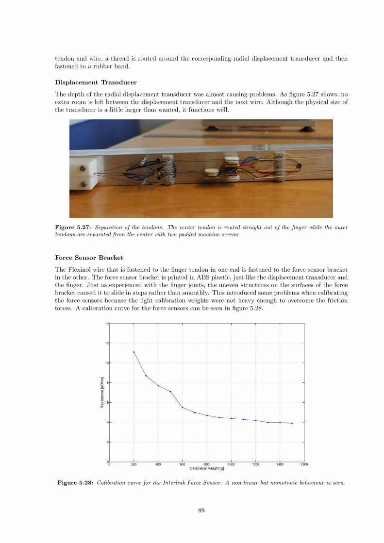
tendon and wire, a thread is routed around the corresponding radial displacement transducer and thenfastened to a rubber band.

Displacement Transducer

The depth of the radial displacement transducer was almost causing problems. As figure 5.27 shows, noextra room is left between the displacement transducer and the next wire. Although the physical size ofthe transducer is a little larger than wanted, it functions well.

Figure 5.27: Separation of the tendons. The center tendon is routed straight out of the finger while the outertendons are separated from the center with two padded machine screws

Force Sensor Bracket

The Flexinol wire that is fastened to the finger tendon in one end is fastened to the force sensor bracketin the other. The force sensor bracket is printed in ABS plastic, just like the displacement transducer andthe finger. Just as experienced with the finger joints, the uneven structures on the surfaces of the forcebracket caused it to slide in steps rather than smoothly. This introduced some problems when calibratingthe force sensors because the light calibration weights were not heavy enough to overcome the frictionforces. A calibration curve for the force sensors can be seen in figure 5.28.

Figure 5.28: Calibration curve for the Interlink Force Sensor. A non-linear but monotonic behaviour is seen.

89

Elastic Displacement Transducer

As described in section 4.5.1, an elastic displacement transducer was considered as an option. However,as figure 5.29 shows, the use of such a transducer is non-trivial. In the figure, the green vertical lines markeach time the elastic transducer was stretched and the black line shows the actual physical stretching. Anegative peak is observed by the first stretching. The peak leasts for about one second before the curvemoves in the correct direction. However, as the graph shows, the transducer does not immediately reflectthe change in displacement. After 10 seconds, the output starts to stabilize, but is slightly increased foranother 15 seconds.

The same behaviour is seen again when the transducer is further stretched at around 32 seconds.Also when decreasing the amount of stretch at 40 seconds, a negative peak is seen. The following peakis caused by a mechanical distortion. The fact that such a small distortion causes a great peak in themeasurement indicates that regulation with such feedback can be difficult. In addition to the slow responseof the transducer, the overall performance is therefore considered too inaccurate for the humanoid fingerapplication.

Figure 5.29: Results from testing of an elastic displacement transducer. The results show that the transducersuffers from large delays. In addition, negative peaks are generated when the transducer is stretched.

5.4.2 Electronics

The electronics schematic of the finger application is presented in section 4.5.2 and its breadboard real-isation can be seen in figure 5.30. The prototype was built on a breadboard to be easily expandable incase of adjustments. The biggest IC is the ATMega32 microcontroller which has a 6-pin programmingconnector situated on its right side. The smaller IC is the MAX202 level shifter, used to convert betweenTTL and ±12V signals for RS232. On the right side of the picture, a 5V regulator can be seen withtwo capacitors for noise filtering of the power supply. On the left side of the picture, three power hexfettransistors can be seen. These are used to drive the Flexinol wires. The large, white ceramic resistorsare used for current measurements.

The electronic design is not very complex, but functioned well for its purpose as prototype base forFlexinol wire regulation. The PWM-frequency of the outputs is desirable to keep as high as possible. Thepower hexfet transistors that are controlled by the PWM-signal will therefore have to keep up with this

90

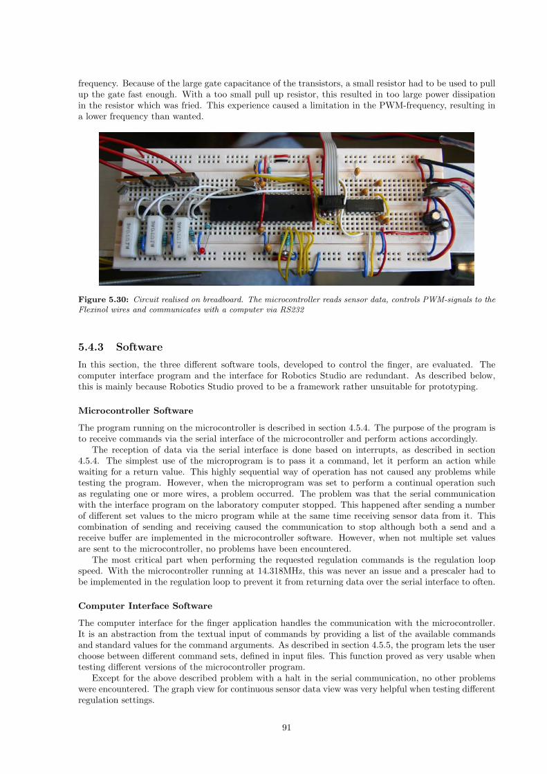
frequency. Because of the large gate capacitance of the transistors, a small resistor had to be used to pullup the gate fast enough. With a too small pull up resistor, this resulted in too large power dissipationin the resistor which was fried. This experience caused a limitation in the PWM-frequency, resulting ina lower frequency than wanted.

Figure 5.30: Circuit realised on breadboard. The microcontroller reads sensor data, controls PWM-signals to theFlexinol wires and communicates with a computer via RS232

5.4.3 Software

In this section, the three different software tools, developed to control the finger, are evaluated. Thecomputer interface program and the interface for Robotics Studio are redundant. As described below,this is mainly because Robotics Studio proved to be a framework rather unsuitable for prototyping.

Microcontroller Software

The program running on the microcontroller is described in section 4.5.4. The purpose of the program isto receive commands via the serial interface of the microcontroller and perform actions accordingly.

The reception of data via the serial interface is done based on interrupts, as described in section4.5.4. The simplest use of the microprogram is to pass it a command, let it perform an action whilewaiting for a return value. This highly sequential way of operation has not caused any problems whiletesting the program. However, when the microprogram was set to perform a continual operation suchas regulating one or more wires, a problem occurred. The problem was that the serial communicationwith the interface program on the laboratory computer stopped. This happened after sending a numberof different set values to the micro program while at the same time receiving sensor data from it. Thiscombination of sending and receiving caused the communication to stop although both a send and areceive buffer are implemented in the microcontroller software. However, when not multiple set valuesare sent to the microcontroller, no problems have been encountered.

The most critical part when performing the requested regulation commands is the regulation loopspeed. With the microcontroller running at 14.318MHz, this was never an issue and a prescaler had tobe implemented in the regulation loop to prevent it from returning data over the serial interface to often.

Computer Interface Software

The computer interface for the finger application handles the communication with the microcontroller.It is an abstraction from the textual input of commands by providing a list of the available commandsand standard values for the command arguments. As described in section 4.5.5, the program lets the userchoose between different command sets, defined in input files. This function proved as very usable whentesting different versions of the microcontroller program.

Except for the above described problem with a halt in the serial communication, no other problemswere encountered. The graph view for continuous sensor data view was very helpful when testing differentregulation settings.

91

Robotics Studio Interface

The interface developed for Microsoft Robotics Studio was an attempt to fit the finger application into anexisting framework for robotic applications as described in section 3.3. However, the framework appearedas cumbersome in use. When programming only a small service such as in this case, very much extrawork had to be put into the strict definition of the communication and data structure of it. These strictdefinitions are of course necessary when dealing with larger systems with many concurrent subsystems,but in a prototype setting, the overhead caused by the framework was greatly slowing the productivitydown.

However, after defining the interface of the service and implementing its functions, a highly reusablemodule is at hand. This is a great benefit for example when different programs use the same hardwaremodules. In practice however, it is often desirable to improve such an interface service. With RoboticsStudio, this involves expanding code that already appears as messy when produced by the code generator.Robotics Studio may be a good choice when developing a large modularized concurrent system, but forthis prototype purpose it simply was too heavy.

92

Chapter 6

Regulation

This chapter focuses closer on the regulation results that were given in the last chapter.

6.1 Finger Regulation

In figure 6.1, the results from regulating a finger can be seen. The curves show the angle of each fingerjoint, and it is clear that oscillations are present. Oscillations are already present when regulating onesingle wire, as described in the previous chapter. However, the oscillations that occur when controllingthe finger are slower than for one single wire. The shape of the finger oscillation looks more pulse shapedthan the sine shape of the single wire control. This behaviour is caused by the mechanical constructionof the finger as the exact same regulation function is used as for the single wire control.

The surface of the finger joints introduces static friction forces. This can be seen when comparing thedeflection curves in figure 6.1 with the force curves in figure 6.2. When looking at the force and deflectioncurve for the PIP-joint at 6s, it is apparent that the force increases at this point, but no deflection ismeasured before one second later. The same seems to happen at around 8s when the force decreases.The PIP-joint starts to stretch when no force is applied to the joint.

6.2 PWM-Controlled

The results from regulation of a single Flexinol wire was given in section 5.2.6. The results revealed thata control of a wire is possible, but far from trivial. Three factors are causing the non-trivial behaviour.

6.2.1 Transformation Curve

The most obvious factor can be seen by looking at the transformation curve of Flexinol in figure 2.13.When heating the wire from a cold state, very little change occurs before the wire reaches a temperatureof ca 70C. Between 70C and 85C, the transformation curve is nonlinear, reaching a contraction rateof about 0.5%. However, the range between 85C and 95C results in contraction from 0.5% to 3.5%.This part of the contraction curve spans over 10C and controls 3% of the available 4% of contraction.This means that very small changes in temperature causes very large changes in contraction. At 90C,such changes can come from air turbulence caused by someone passing by, or a window being open. Thisbehaviour is also reflected by the different curves in figure 5.22. When looking at the four lower stepsand the four upper steps, lower oscillation amplitudes and frequencies can be observed.

To compensate for this behaviour, accurate sensor feedback and current control is needed. By devel-oping a model for the wire contraction, a better regulation could possibly be done.

6.2.2 Hysteresis

The hysteresis of the Flexinol wires is already mentioned in section 2.3.1 and can clearly be seen infigure 2.13. The hysteresis can easily be modelled for a complete cycle of heating and cooling, but itis unclear from the contraction curve what happens if the heating is stopped at around 2% and thenthe wire is cooled. Does this lead to a smaller hysteresis or is the behaviour unchanged? This question

93

Figure 6.1: Regulation of a finger where each joint has a set value of 45. The curves show the angle of eachjoint. Oscillations of about ±10 are observed

Figure 6.2: Force measurements from the same regulation as figure 6.1. The oscillations are also seen as changesin force. The MCP-joint exerts the largest forces because of its tendon fastening

94

is difficult to answer as no temperature measurements have been performed during this thesis due totechnical difficulties and the small size of the wire. The hysteresis behaviour makes it necessary to keeprecord of the current state of the wire while regulating. A regulation model will in other words need toknow whether or not it must expect hysteresis behaviour when loaded with a new set point.

6.2.3 Delay

The third factor that makes regulation non-trivial is the delay that occurs after a change in currentand before a change in contraction. The delay is caused by the time needed to heat the wire. Whenincreasing or decreasing the current flowing through the Flexinol wire, the heating or cooling of the wirebegins immediately, but it takes some time before the process is completed. As the curves in figure 5.21show, a rather large overshoot can be observed when controlling the wire from 0% contraction to a givencontraction rate. This is caused by the overall delay in the system, including both regulation and wiredelay. The proportional regulation used in section 5.2.6 is probably not the best solution to regulate thewire, because it does not predict any behaviour like this. It increases the output until it reaches its setvalue and then decreases the output to work against the overshoot. However, as this system contains arather long delay, more overshoot than wanted is observed. figure 6.3 shows on contraction curve of aFlexinol wire. A delay of 2.5s is seen between the start and the end of the contraction. This is 2.5 timeslonger than specified in the Flexinol datasheet.

Figure 6.3: One contraction cycle of Flexinol with high resolution. A delay of ca 2.5s can be seen when contractingthe wire. This is 2.5 times more than specified in the datasheet

6.3 Regulation Models by Other Authors

As already mentioned, some approaches have already been performed by other authors to investigate thepossibility to regulate the contraction rate of Flexinol.

Grant and Hayward present a working two-stage regulation mechanism in [71]. An antagonistic setupwith two high strain SMA actuators [22] is controlled to exert a specified force. The two-stage controllerfirst uses a high regulation factor to kick-start the regulation. When a threshold value is reached, a

95

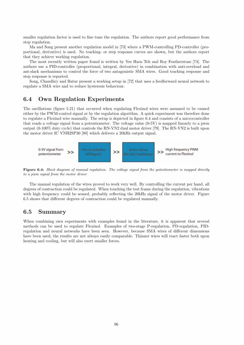
smaller regulation factor is used to fine tune the regulation. The authors report good performance fromstep regulation.

Ma and Song present another regulation model in [73] where a PWM-controlling PD-controller (pro-portional, derivative) is used. No tracking- or step response curves are shown, but the authors reportthat they achieve working regulation.

The most recently written paper found is written by Yee Harn Teh and Roy Featherstone [74]. Theauthors use a PID-controller (proportional, integral, derivative) in combination with anti-overload andant-slack mechanisms to control the force of two antagonistic SMA wires. Good tracking response andstep response is reported.

Song, Chaudhry and Batur present a working setup in [72] that uses a feedforward neural network toregulate a SMA wire and to reduce hysteresis behaviour.

6.4 Own Regulation Experiments

The oscillations (figure 5.21) that occurred when regulating Flexinol wires were assumed to be causedeither by the PWM-control signal or by the regulation algorithm. A quick experiment was therefore doneto regulate a Flexinol wire manually. The setup is depicted in figure 6.4 and consists of a microcontrollerthat reads a voltage signal from a potentiometer. The voltage value (0-5V) is mapped linearly to a pwmoutput (0-100% duty cycle) that controls the RN-VN2 dual motor driver [79]. The RN-VN2 is built uponthe motor driver IC VNH2SP30 [80] which delivers a 20kHz output signal.

Figure 6.4: Block diagram of manual regulation. The voltage signal from the potentiometer is mapped directlyto a pwm signal from the motor driver

The manual regulation of the wires proved to work very well. By controlling the current per hand, alldegrees of contraction could be regulated. When touching the test frame during the regulation, vibrationswith high frequency could be sensed, probably reflecting the 20kHz signal of the motor driver. Figure6.5 shows that different degrees of contraction could be regulated manually.

6.5 Summary

When combining own experiments with examples found in the literature, it is apparent that severalmethods can be used to regulate Flexinol. Examples of two-stage P-regulation, PD-regulation, PID-regulation and neural networks have been seen. However, because SMA wires of different dimensionshave been used, the results are not always easily comparable. Thinner wires will react faster both uponheating and cooling, but will also exert smaller forces.

96

Figure 6.5: Manual regulation of a Flexinol wire. The curve shows clearly that regulation is feasible

97

98

Chapter 7

Future Work

Flexinol wires have been on the market for several years, but very few real life applications have beenfound during this thesis. It seems like little basis research has been done in the field, maybe one of thereasons that make the inclusion of Flexinol in larger systems rare. This thesis aims to design a humanoidfinger which is to be actuated with Flexinol wires and some tests of Flexinol had to be performed beforethe finger could be designed. During the scope of the thesis, the goal was to develop a working finger.To achieve this goal, some milestones had to be reached faster than with another time perspective.This chapter therefore focuses on the aspects of the thesis that deserves more attention in addition tointeresting problems that were discovered during development.

7.1 Flexinol Testing

The results from testing of Flexinol wires in a test frame show that this is very time consuming work.Wires have to be changed and data sets need to be analyzed. As an example for this is the testing witha small load where one wire lasted for 40 days. To get enough empirical data to conclude exactly howFlexinol wires can be used in the best way, many more tests should be performed. This would includebuilding a bigger test frame so that many equal test setups can be run in parallel. Deflection transducerswith a working range of more than 50mm should also be used so that the wires don’t have to be tightenedduring runtime. A solution could be to use radial displacement transducers for all wires.

A fastening mechanism should also be developed to fasten the fixated Flexinol wire in a more gentleway when testing. In this way, more accurate measures of how long the wire lasts can be collected.Although the use of a Flexinol wire as antagonist was abandoned during this thesis, the concept shouldalso be closer investigated.

Attempts were made to measure how much a wire had been stretched after it had broken. This provedto be very difficult as the wires broke in different contraction states. An attempt was made to stretchthe wire and then measure, but this resulted in the wire also breaking other places. This challenge couldmaybe be overcome by always measuring the wires in a contracted state, thus not having to stretch thewire after it is broken. This would reaveal information about how much a wire can be stretched beforeit breaks. In this way a better prediction can hopefully be done.

7.2 Regulation

During this thesis, only one regulation approach is done in addition to an successful attempt to manuallyregulate Flexinol. A regulation algorithm for a single Flexinol wire should be developed in the future. Ifsuch an algorithm is able to control a single wire without oscillations, chances are good that a finger alsocan be regulated.

7.3 Developed Finger

The prototyped finger was printed in ABS-plastic and the results from this process are described insection 5.3. The finger was designed with a size ratio of 3:1. A second finger should be produced in a

99

1:1 ratio and preferably in metal to get even surfaces to keep friction at a minimum. To achieve thetrue movements of the human finger, the MCP-joint should also support adduction and abduction asdescribed in section 4.4.1. In this way, the kinetic sketch of the finger would be the same as the humanfinger except from tendon routing.

Touch sensors or force sensors could be mounted on the inside of the fingers, making grasping opera-tions possible. By also producing the finger with a rubber like material on the inside, grasping would beeven more feasible. If good control of one finger is achieved, it would be very interesting to see if a wholehand could be assembled from the fingers. In this case, a thumb should also be developed, a non-trivialtask both mechanically and in terms of regulation.

7.4 Electronics

The electronic circuits built during the thesis were realized on bread board. For a second prototype,it would be preferable with a smaller realization on a printed circuit board (PCB). It would also bepreferable with a much higher PWM-frequency for the output, alternatively could a motor driver like theL6205 [81] from STMicroelectronics be used to control the current flowing through the Flexinol wires. Inthis way, the current measurements would probably be much more accurate be cause of the eliminationof the PWM-shaped current flow.

100

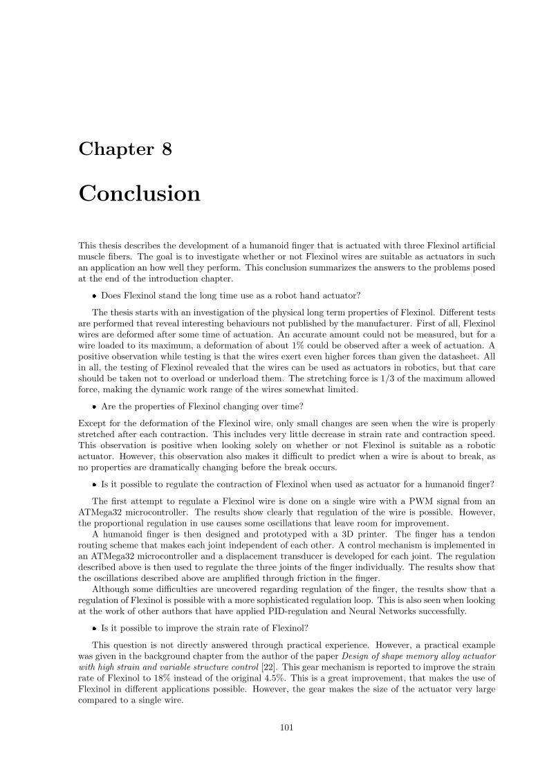
Chapter 8

Conclusion

This thesis describes the development of a humanoid finger that is actuated with three Flexinol artificialmuscle fibers. The goal is to investigate whether or not Flexinol wires are suitable as actuators in suchan application an how well they perform. This conclusion summarizes the answers to the problems posedat the end of the introduction chapter.

Does Flexinol stand the long time use as a robot hand actuator?

The thesis starts with an investigation of the physical long term properties of Flexinol. Different testsare performed that reveal interesting behaviours not published by the manufacturer. First of all, Flexinolwires are deformed after some time of actuation. An accurate amount could not be measured, but for awire loaded to its maximum, a deformation of about 1% could be observed after a week of actuation. Apositive observation while testing is that the wires exert even higher forces than given the datasheet. Allin all, the testing of Flexinol revealed that the wires can be used as actuators in robotics, but that careshould be taken not to overload or underload them. The stretching force is 1/3 of the maximum allowedforce, making the dynamic work range of the wires somewhat limited.

Are the properties of Flexinol changing over time?

Except for the deformation of the Flexinol wire, only small changes are seen when the wire is properlystretched after each contraction. This includes very little decrease in strain rate and contraction speed.This observation is positive when looking solely on whether or not Flexinol is suitable as a roboticactuator. However, this observation also makes it difficult to predict when a wire is about to break, asno properties are dramatically changing before the break occurs.

Is it possible to regulate the contraction of Flexinol when used as actuator for a humanoid finger?

The first attempt to regulate a Flexinol wire is done on a single wire with a PWM signal from anATMega32 microcontroller. The results show clearly that regulation of the wire is possible. However,the proportional regulation in use causes some oscillations that leave room for improvement.

A humanoid finger is then designed and prototyped with a 3D printer. The finger has a tendonrouting scheme that makes each joint independent of each other. A control mechanism is implemented inan ATMega32 microcontroller and a displacement transducer is developed for each joint. The regulationdescribed above is then used to regulate the three joints of the finger individually. The results show thatthe oscillations described above are amplified through friction in the finger.

Although some difficulties are uncovered regarding regulation of the finger, the results show that aregulation of Flexinol is possible with a more sophisticated regulation loop. This is also seen when lookingat the work of other authors that have applied PID-regulation and Neural Networks successfully.

Is it possible to improve the strain rate of Flexinol?

This question is not directly answered through practical experience. However, a practical examplewas given in the background chapter from the author of the paper Design of shape memory alloy actuatorwith high strain and variable structure control [22]. This gear mechanism is reported to improve the strainrate of Flexinol to 18% instead of the original 4.5%. This is a great improvement, that makes the use ofFlexinol in different applications possible. However, the gear makes the size of the actuator very largecompared to a single wire.

101

Is it possible to use multiple Flexinol wires in parallel?

Whether or not a parallel use of Flexinol wires is possible is not answered in this thesis through experi-ments. However, the experiences gained through experiments with single Flexinol wires have shown thatthis may be complicated. In many setups, variances are seen between different wires regarding how fastand how much they are stretched. These differences are mainly caused by the use of different loads for thewires. This implicates that in a parallel setup, all wires should be equally loaded. To achieve this, a veryaccurate and homogenous fastening of each wire has to be performed. In [21], a parallel bundle actuatoris presented. However, the article does not report whether or not the parallel wires behave homogenous.

102

Bibliography

[1] K.B. Fite, T.J. Withrow, Xiangrong Shen, K.W. Wait, J.E. Mitchell, and M. Goldfarb. A gas-actuated anthropomorphic prosthesis for transhumeral amputees. Robotics, IEEE Transactions on,24(1):159–169, Feb. 2008.

[2] Kathryn J. De Laurentis and Constantinos Mavroidis. Mechanical design of a shape memory alloyactuated prosthetic hand. IOS Press, Technology and Health Care, 10(2):91–106, 2002.

[3] B. Massa, S. Roccella, M.C. Carrozza, and P. Dario. Design and development of an underactuatedprosthetic hand. In Robotics and Automation, 2002. Proceedings. ICRA ’02. IEEE InternationalConference on, volume 4, pages 3374–3379 vol.4, 2002.

[4] Kenji Kaneko, Kensuke Harada, and Fumio Kanehiro. Development of multi-fingered hand forlife-size humanoid robots. In ICRA, pages 913–920. IEEE, 2007.

[5] Kiyoshi Hoshino and Ichiro Kawabuchi. Mechanism of humanoid robot arm with 7 dofs havingpneumatic actuators. IEICE Trans Fundamentals, E89-A(11):3290–3297, 2006.

[6] Naoki Fukaya, Shigeki Toyama, Tamim Asfour, and Rdiger Dillmann. Design of the tuat/karlsruhehumanoid hand, May 17 2000.

[7] Shadow Robot Company. Design of a dextrous hand for advanced clawar applicationswww.shadowrobot.com/downloads/dextrous hand final.pdf.

[8] A. Kargov, T. Asfour, C. Pylatiuk, R. Oberle, H. Klosek, S. Schulz, K. Regenstein, G. Bretthauer,and R. Dillmann. Development of an anthropomorphic hand for a mobile assistive robot. Rehabil-itation Robotics, 2005. ICORR 2005. 9th International Conference on, pages 182–186, June-1 July2005.

[9] H. Kawasaki, T. Komatsu, and K. Uchiyama. Dexterous anthropomorphic robot hand with dis-tributed tactile sensor: Gifu hand ii. Mechatronics, IEEE/ASME Transactions on, 7(3):296–303,Sep 2002.

[10] Bertrand Tondu, Serge Ippolito, Jeremie Guiochet, and A. Daidie. A seven-degrees-of-freedom robot-arm driven by pneumatic artificial muscles for humanoid robots. I. J. Robotic Res, 24(4):257–274,2005.

[11] Bielefeld University. www.techfak.uni-bielefeld.de/ags/ni/projects/m6setup/hand.html.

[12] B. Almasri and F. B. Ouezdou. New design of one motor driven under actuated humanoid hand.Intelligent Robots and Systems, 2007. IROS 2007. IEEE/RSJ International Conference on, pages1491–1496, Oct. 29 2007-Nov. 2 2007.

[13] Karsten Berns, Tamim Asfour, and Rudiger Dillmann. Armar an anthropomorphic arm for humanoidservice robot. In ICRA, pages 702–707, 1999.

[14] Tamim Asfour, Karsten Berns, and Rudiger Dillmann. The humanoid robot armar: Design andcontrol. pages 7–8, 2000.

[15] T. Dutta and T. Chau. A feasibility study of flexinol as the primary actuator in a prosthetic hand.In IEEE CCECE 2003, Canadian Conference on Electrical and Computer Engineering, volume 3,pages 1449–1452 vol.3, 2003.

103

[16] F. Gori, D. Carnevale, A. Doro Altan, S. Nicosia, and Pennestrı. A new hysteretic behavior in theelectrical resistivity of flexinol shape memory alloys versus temperature. International Journal ofThermophysics, 27(3):866–879, May 2006.

[17] H.H. Selden, B.; Kyu-Jin Cho; Asada. Segmented binary control of shape memory alloy actuatorsystems using the peltier effect. Robotics and Automation, 2004. Proceedings. ICRA ’04. 2004 IEEEInternational Conference on, 5:4931–4936 Vol.5, 26 April-1 May 2004.

[18] M G Faulkner T B Wolfe (nee Bunton) and J Wolfaardt. Development of a shape memory alloyactuator for a robotic eye prosthesis. Smart Materials and Structures, 14(4):759–768, 2005.

[19] W M Ostachowicz A J Zak, M P Cartmell and M Wiercigroch. One-dimensional shape memoryalloy models for use with reinforced composite structures. Smart Materials and Structures, 12(3):338–346, 2003.

[20] Pavel L. Potapov and Edson P. Da Silva. Time response of shape memory alloy actuators. Journalof Intelligent Material Systems and Structures, 11(2):125–134, 2000.

[21] Michael J. Mosley and Constantinos Mavroidis. Design and dynamics of a shape memory alloy wirebundle actuator, 1999.

[22] V. Grant, D.; Hayward. Design of shape memory alloy actuator with high strain and variablestructure control. Robotics and Automation, 1995. Proceedings., 1995 IEEE International Conferenceon, 3:2305–2312 vol.3, 1995.

[23] Wikipedia. Hand en.wikipedia.org/wiki/Hand, Aug 2008.

[24] Wikipedia. Muscle en.wikipedia.org/wiki/Muscle, Oct 2008.

[25] Johannes Sobotta. Atlas of Human Anatomy, Volume 1 Head, Neck, Upper Limb. Urban & Fischer,2001.

[26] John Lin, Ying Wu, and T.S. Huang. Modeling the constraints of human hand motion. HumanMotion, 2000. Proceedings. Workshop on, pages 121–126, 2000.

[27] Gates Corporation. Introduction to hydraulics, www.gates.com/common/downloads-/files/Gates/autoEducation/428-7153.pdf.

[28] S. Schulz, C. Pylatiuk, and G. Bretthauer. A new ultralight anthropomorphic hand. In Roboticsand Automation, 2001. Proceedings 2001 ICRA. IEEE International Conference on, volume 3, pages2437–2441 vol.3, 2001.

[29] Jozef Barycki, Miroslaw Ganczarek, Waclaw Kollek, Tadeusz Mikulczynski, and Zdzislaw Samsonow-icz. Performances of high-speed pneumatic drive with self-acting impulse valve. Mechanism andMachine Theory, 39(6):657–663, June 2004.

[30] F. Oaerden and D. Lefeber. Pneumatic artificial muscles: actuators for robotics and automation.European Journal of Mechanical and Environmental Engineering, 47:11–21, 2002.

[31] Hitec RCD. Servo list, www.hitecrcd.com/product file/file/124/Servo Chart.pdf.

[32] Hitec RCD. Datasheet hitec hsr-8498hb, www.hitecrcd.com/product file/file/109/HSR-8498HB GENERAL SPECIFICATION 050623.pdf.

[33] Johnson Electric. Datasheet ledex tubular solenoids, www.ledex.com/ltr2/access.php?file=pdf/Tubular Section M.pdf.

[34] Dialight BLP. Datasheet black night series 124, www.blpcomp.com/products/datasheet/bkseries124.pdf.

[35] C. Mavroidis. Development of advanced actuators using shape memory alloys and electrorheologicalfluids. Research in Nondestructive Evaluation, 14(1):1–32, January 2002.

[36] Dynnaloy, Inc. Flexinol actuator wire heat curves, www.dynalloy.com/docs/25ksi90C1.pdf.

104

[37] Dynnaloy, Inc. Technical characteristics of flexinol actuator wire,www.dynalloy.com/docs/TCF1140RevD.pdf.

[38] R.A. Russell and R.B. Gorbet. Improving the response of sma actuators. Robotics and Automation,1995. Proceedings., 1995 IEEE International Conference on, 3:2299–2304 vol.3, May 1995.

[39] N. Troisfontaine, P. Bidaud, and M. Larnicol. Optimal design of micro-actuators based on sma wires.Smart Material Structures, 8:197–203, April 1999.

[40] N. Lakhkar, M. Hossain, and D. Agonafer. Cfd modeling of a thermoelectric device for electronicscooling applications. Thermal and Thermomechanical Phenomena in Electronic Systems, 2008.ITHERM 2008. 11th Intersociety Conference on, pages 889–895, May 2008.

[41] Custom Thermoelectric. Thermoelectric cooler 00711-5l31-03cawww.customthermoelectric.com/tecs/pdf/00711-5L31-03CA spec sht.pdf.

[42] KRYOTHERM. Thermoelectric cooler snowball-71 www.eureca.de/pdf/cooling/peltier-elements/SnowBall-71.pdf.

[43] Dynnaloy, Inc. Information on the electrostem® valve, www.dynalloy.com/docs/electrostem.pdf.

[44] Jonathan W. Mills. Stiquito: A small, simple, inexpensive hexapod robot part 1. locomotion andhard-wired control. Technical report, Computer Science Department; Indiana University; Blooming-ton, Indiana 47405, April 21 1999.

[45] J.M. McClain, A.; Conrad. Software design of the stiquito micro robot. Proceedings IEEE SoutheastCon, 8-10 April 2005., pages 143–147, 2005.

[46] Alberto Paiva and Marcelo Amorim Savi. An overview of constitutive models for shape memoryalloys. Mathematical Problems in Engineering, 2006:30 pages, 2006.

[47] Qin Chang-jun, Ma Pei-sun, and Yao Qin. A prototype micro-wheeled-robot using sma actuator.Sensors and Actuators A: Physical, 113(1):94–99, June 2004.

[48] Technicsche Universitat Darmstadt. Elektroaktive polymere, www.emk.tu-darmstadt.de/institut/fachgebiete/m ems/forschung/dielektrische polymeraktoren.

[49] Yoseph Bar-Cohen. Bionic humans using eap as artificial muscles reality and challenges. InternationalJournal of Advanced Robotic Systems, 1(3):217–222, November 08 2004.

[50] Kentaro Takagi, Masanori Yamamura, Zhi-Wei Luo, Masaki Onishi, Shinya Hirano, Kinji Asaka,and Yoshikazu Hayakawa. Development of a rajiform swimming robot using ionic polymer artificialmuscles. Intelligent Robots and Systems, 2006 IEEE/RSJ International Conference on, pages 1861–1866, Oct. 2006.

[51] J.D.W. Madden, N.A. Vandesteeg, P.A. Anquetil, P.G.A. Madden, A. Takshi, R.Z. Pytel, S.R.Lafontaine, P.A. Wieringa, and I.W. Hunter. Artificial muscle technology: physical principles andnaval prospects. Oceanic Engineering, IEEE Journal of, 29(3):706–728, July 2004.

[52] Jaewook Ryu, Younkoo Jeong, Younghun Tak, Byungmok Kim, Byungkyu Kim, and Jong-Oh Park.A ciliary motion based 8-legged walking micro robot using cast ipmc actuators. Micromechatronicsand Human Science, 2002. MHS 2002. Proceedings of 2002 International Symposium on, pages 85–91, 2002.

[53] N.N. Pak, S. Scapellato, G. La Spina, G. Pernorio, A. Menciassi, and P. Dario. Biomimetic designof a polychaete robot using ipmc actuator. Biomedical Robotics and Biomechatronics, 2006. BioRob2006. The First IEEE/RAS-EMBS International Conference on, pages 666–671, 0-0 0.

[54] M. Shahinpoor, T. Xue, and J. O. Simpson. Ionic polymer-metal composites (ipmc) as biomimeticsensors and actuators, April 19 2001.

[55] Shuxiang Guo, T. Fukuda, and K. Asaka. A new type of fish-like underwater microrobot. Mecha-tronics, IEEE/ASME Transactions on, 8(1):136–141, March 2003.

105

[56] Dominiek Reynaerts and Hendrik Van Brussel. Design aspects of shape memory actuators. Mecha-tronics, 8(6):635–656, August 1998.

[57] Anaheim Automation. Stepper sealed high torque motor - 42n65 serieswww.anaheimautomation.com/stepper-sealed-high-torque-motor-42N65.aspx.

[58] Wikipedia. Power-to-weight ratio en.wikipedia.org/wiki/Power-to-weight ratio, Oct 2008.

[59] K. Ikuta. Micro/miniature shape memory alloy actuator. Robotics and Automation, 1990. Proceed-ings., 1990 IEEE International Conference on, pages 2156–2161 vol.3, May 1990.

[60] Y. Bar-Cohen, T. Xue, M. Shahinpoor, J. O. Simpson, and J. Smith. Low-mass muscle actuatorsusing electroactive polymers (eap). Smart materials and technologies; Proceedings of the Meeting,San Diego, CA; UNITED STATES; 4-5 Mar., 3324:218–223, July 1998.

[61] John D. Madden, Ryan A. Cush, Tanya S. Kanigan, and Ian W. Hunter. Fast contracting polypyrroleactuators. Synthetic Metals, 113(1-2):185–192, June 2000.

[62] John D. Madden, Peter G. Madden, and Ian W. Hunter. Polypyrrole actuators: modeling andperformance. Smart Structures and Materials 2001: Electroactive Polymer Actuators and Devices,4329(1):72–83, 2001.

[63] Ledex. Datasheet ledex low profile 8ecm www.ledex.com/ltr2/access.php?file=pdf/LowProfile 8ECM.pdf.

[64] Ledex. Datasheet ledex pull tubular 13x14mm www.ledex.com/ltr2/access.php?file=pdf/Tubular 13x14 Pull.pdf.

[65] RDP Group. D5w submersible lvdt displacement transducer www.rdpe.com/ex/d5w.htm.

[66] RDP Group. How it works - lvdt www.rdpe.com/displacement/lvdt/lvdt-principles.htm.

[67] Interlink Electronics. Force sensing resistor www.interlinkelectronics.com/force sensors/technologies/fsr.html.

[68] Atmel. Datasheet atmel avr atmega32, www.atmel.com/dyn/resources/prod documents/doc2503.pdf.

[69] Keithley Instruments Inc. Model kusb-3100 user’s manual www.keithley.com/data?asset=50306.

[70] Microsoft. Microsoft robotics studio user guide, msdn.microsoft.com/en-us/library/bb483024.aspx.

[71] D. Grant and V. Hayward. Constrained force control of shape memory alloy actuators. Robotics andAutomation, 2000. Proceedings. ICRA ’00. IEEE International Conference on, 2:1314–1320 vol.2,2000.

[72] G. Song, V. Chaudhry, and C. Batur. Precision tracking control of shape memory alloy actuatorsusing neural networks and a sliding-mode based robust controller. Smart Material Structures, 12:223–231, April 2003.

[73] N. Ma and G. Song. Control of shape memory alloy actuator using pulse width modulation. SmartMaterial Structures, 12:712–719, October 2003.

[74] Yee Harn Teh and Roy Featherstone. An architecture for fast and accurate control of shape memoryalloy actuators. The International Journal of Robotics Research, 27(5):595–611, 2008.

[75] Infineon. Datasheet bss98 n-channel sipmos small-signal transistorwww.infineon.convergy.de/upload/documents/techdoc/GF 52/bss98.pdf.

[76] International Rectifier. Datasheet irf95420n single p-channel hexfet power mosfetwww.irf.com/product-info/datasheets/data/irf9540n.pdf.

[77] Keithley Instruments Inc. Dataacq sdk user’s manual www.keithley.com/data?asset=50242.

[78] Maxim IC. Datasheet for max202 datasheets.maxim-ic.com/en/ds/MAX200-MAX213.pdf.

106

[79] robotikhardware.de. Datasheet www.shop.robotikhardware.de/shop/catalog/product info.php?cPath=65&products id=112.

[80] STMicroelectronics. Datasheet fully integrated h-bridge motordriverwww.st.com/stonline/products/literature/ds/10832/vnh2sp30-e.pdf.

[81] STMicroelectronics. Datasheet for l6205 motor driver www.st.com/stonline/products/literature/ds/7616/l6205.htm.

107

108

Appendix A

Code attachment

A.1 Software for Test Frame Control and Measurement

The below code is the implementation of the program described in section 4.3.1. An evaluation of theprogram was given in section 5.2.1.

Listing A.1: Program Loader (Program.cs)

1 ı¿using System ;2 using System . Co l l e c t i on s . Generic ;3 using System . Linq ;4 using System . Windows . Forms ;56 namespace f l ex ino lRiggSansRS 7 stat ic c lass Program 8 /// <summary>9 /// The main entry point f o r the app l i c a t i on .

10 /// </summary>11 [ STAThread ]12 stat ic void Main ( ) 13 Appl i cat ion . Enab leVi sua lSty l e s ( ) ;14 Appl i cat ion . SetCompatibleTextRenderingDefault ( f a l s e ) ;15 Appl i cat ion . Run(new Flex ino lRigg ( ) ) ;16 17 18

Listing A.1: Program Loader (Program.cs)

Listing A.2: Main program (FlexinolRigg.cs)

1 ı¿using System ;2 using System . Co l l e c t i on s . Generic ;3 using System . ComponentModel ;4 using System . Data ;5 using System . Drawing ;6 using System . Text ;7 using System . Windows . Forms ;8 using System . Diagnos t i c s ;9

10 namespace f l ex ino lRiggSansRS 11 public p a r t i a l c lass Flex ino lRigg : Form 12 public string ve r s i on = ” Flex ino lRigg v1 . 0 ” ;1314 private double [ ] l a s tA in = 0 , 0 , 0 , 0 , 0 , 0 , 0 , 0 ;15 private bool [ ] lastDout = fa lse , fa lse , fa lse , fa lse , fa lse , fa lse , fa lse , f a l s e ;16 private double [ ] nu l lAin = 0 , 0 , 0 , 0 , 0 , 0 , 0 , 0 ;1718 private ngraph [ ] graphs = new ngraph [ 5 ] ;19 private Color [ ] l i n e c o l o r s = new Color [ ] 20 Color . Red ,21 Color . Blue ,22 Color . Green ,23 Color . Black ,24 Color . Purple ,25 Color . Yellow ,26 Color . Brown ,27 Color . Magenta ,28 Color . Cyan ,29 Color . DarkGray ,30 Color . Orange ,31 Color . LightGray ;3233 private setup setup ;34 private DataGridView [ ] dg ;35 private GroupBox [ ] gb ;36 private Button [ ] btnZero ;37 private dataWriter wr i t e r ;3839 private Kusb3100 kusb ;40 private bool doMeasurementLoop = f a l s e ;

109

41 private bool doReloadDoutProg = f a l s e ;42 private bool [ ] r e loadIndex = new bool [ 6 ] ;4344 public Flex ino lRigg ( ) 45 In i t ia l i zeComponent ( ) ;4647 setup = new setup ( ”c :\\ Serv iceSetup\\ f l ex ino lFrame . txt ” ) ;48 4950 private void Flex ino lRigg Load ( object sender , EventArgs e ) 51 this . Text = ver s i on ;52 dg = new DataGridView [ ] dg1 , dg2 , dg3 , dg4 , dg5 ;53 gb = new GroupBox [ ] grpWire1 , grpWire2 , grpWire3 , grpWire4 , grpWire5 ;54 btnZero = new Button [ ] btnZero1 , btnZero2 , btnZero3 , btnZero4 , btnZero5 ;5556 this . FormClosing += new FormClosingEventHandler ( FlexinolRigg FormClos ing ) ;57 try 58 kusb = new Kusb3100 ( ) ;59 catch ( Exception ex ) 60 System . Windows . Forms . MessageBox . Show( ”Connection to Keith ley KUSB−3100 f a i l e d : ” + ex . Message ,

” Error ” , System . Windows . Forms . MessageBoxButtons .OK) ;61 this . Close ( ) ;62 6364 int c o l o r c n t = 0 ;6566 int w = panGraph . Width / 3 ;67 int h = panGraph . Height / 2 ;6869 string [ ] p r e f i x = new string [ 5 ] ;7071 for ( int i = 0 ; i < 5 ; i++) 72 dg [ i ] . RowCount = setup . g e t In t eg e r ( ” wire ” + i + ” cnt ” ) ;73 gb [ i ] . Text = setup . g e tS t r ing ( ” wire ” + i + ”name” ) ;74 p r e f i x [ i ] = setup . g e tS t r ing ( ” wire ” + i + ” . p r e f i x ” ) + ” ” ;75 string [ ] names = new string [ dg [ i ] . RowCount ] ;76 double [ ] va lues = new double [ dg [ i ] . RowCount ] ;7778 for ( int j = 0 ; j < dg [ i ] . RowCount ; j++)79 dg [ i ] [ 0 , j ] . Value = setup . g e tS t r ing ( ” wire ” + i + ” . ” + j ) ;80 dg [ i ] [ 1 , j ] . Value = ”” ;81 names [ j ] = setup . g e tS t r ing ( ” wire ” + i + ” . ” + j ) ;82 c o l o r c n t ++;83 va lues [ j ] = 0 . 0 ;84 85 btnZero [ i ] . C l i ck += btnZero Cl ick ;8687 graphs [ i ] = new ngraph (88 names ,89 se tup . g e t In t eg e r ( ”xmax” ) ,90 se tup . g e tS t r ing ( ” wire ” + i + ”name” ) + ” ( [ cm] / [N] / [V] ) ” ,91 se tup . g e tS t r ing ( ” dump folder ” ) + i + ” . png” ) ;929394 i f ( i < 3) 95 panGraph . Contro ls .Add( graphs [ i ] ) ;9697 graphs [ i ] . Location = new Point (w * i , 0) ;98 99 else

100 panGraph . Contro ls .Add( graphs [ i ] ) ;101 graphs [ i ] . Location = new Point (w * ( i−3) , h) ;102 103104 graphs [ i ] . S i z e = new S i ze (w, h) ;105 // graphs [ i ] . addValues ( values , DateTime .Now) ;106 107108 wr i t e r = new dataWriter ( p re f i x , s e tup . g e t In t eg e r ( ” f i l i n t e r v a l l ” ) , s e tup . g e tS t r ing ( ” da ta f o l d e r ” ) ) ;109110 l s t S t a t u s . Location = new Point ( panGraph . Le f t + w * 2 + 35 , panGraph . Top + h + 37) ;111 l s t S t a t u s . Height = graphs [ 0 ] . Height − 59 ;112 l s t S t a t u s . Width = graphs [ 0 ] . Width − 49 ;113 l s t S t a t u s . BorderStyle = BorderStyle . F ixedS ing le ;114115116 se tS ta tu s ( ” FlexinolRiggSansRS loaded ” ) ;117118 119120 void FlexinolRigg FormClos ing ( object sender , FormClosingEventArgs e ) 121 i f ( doMeasurementLoop ) e . Cancel = true ;122 Debug . WriteLine ( ”FormClosing ( ” + e . Cancel . ToString ( ) + ” ) ” ) ;123 i f ( e . Cancel ) s e tS ta tu s ( ”Stop measurement be fo r e c l o s i n g the form” ) ;124 125126 // de l ega t e void SetStatusCal lback ( s t r i n g s ta tu s ) ;127 private void s e tS ta tu s ( string s t a tu s ) 128 /* i f ( l s t S t a t u s . InvokeRequired ) 129 SetStatusCal lback d = new SetStatusCal lback ( s e tS ta tu s ) ;130 l s t S t a t u s . Invoke (d , new ob j ec t [ ] s t a tu s ) ;131 e l s e 132 */133 s ta tu s = DateTime .Now + ” − ” + sta tu s ;134 l s t S t a t u s . Items . I n s e r t (0 , s t a tu s ) ;135136 while ( l s t S t a t u s . Items . Count > 50) 137 l s t S t a t u s . Items . RemoveAt( l s t S t a t u s . Items . Count − 1) ;138 139 //140 141142 private void btnZero Cl ick ( object sender , EventArgs e ) 143 int i = Array . IndexOf ( btnZero , ( Button ) sender ) ;144145 int chnum ;146 string ch ;147148 for ( int j = 0 ; j < se tup . g e t In t eg e r ( ” wire ” + i + ” cnt ” ) ; j++) 149 ch = setup . g e tS t r ing ( se tup . g e tS t r ing ( ” wire ” + i + ” . ” + j + ” ch ” ) + ” ch ” ) ;150 i f ( ch . StartsWith ( ”Ain” ) ) 151 chnum = int . Parse ( ch . Substr ing (3 , 1) ) ;152 nul lAin [ chnum ] = las tAin [ chnum ] ;

110

153 154 155 156157 private void setValue ( string [ ] v , int i ) 158 for ( int j = 0 ; j < dg [ i ] . RowCount ; j++) dg [ i ] [ 1 , j ] . Value = v [ j ] ;159 160161 private void startToolStr ipMenuItem Cl ick ( object sender , EventArgs e ) 162 doMeasurement ( ) ;163 164165 private void stopToolStr ipMenuItem Click ( object sender , EventArgs e ) 166 stopToolStripMenuItem . Enabled = f a l s e ;167 doMeasurementLoop = f a l s e ;168 169170 private void exitProgramToolStripMenuItem Click ( object sender , EventArgs e ) 171 this . Close ( ) ;172 173174175 private void doMeasurement ( ) 176 for ( int i = 0 ; i < 6 ; i++) re loadIndex [ i ] = f a l s e ;177178 se tS ta tu s ( ”Measurement s t a r t ed ” ) ;179180 startToolStr ipMenuItem . Enabled = f a l s e ;181 stopToolStripMenuItem . Enabled = true ;182 exitProgramToolStripMenuItem . Enabled = f a l s e ;183 reloadDoutValuesToolStripMenuItem . Enabled = true ;184185 reloadDoutValuesForWire1ToolStripMenuItem . Enabled = true ;186 reloadDoutValuesForWire2ToolStripMenuItem . Enabled = true ;187 reloadDoutValuesForWire3ToolStripMenuItem . Enabled = true ;188 reloadDoutValuesForWire4ToolStripMenuItem . Enabled = true ;189 reloadDoutValuesForWire5ToolStripMenuItem . Enabled = true ;190191 doMeasurementLoop = true ;192 int mean ms = setup . g e t In t eg e r ( ”mean ms” ) ;193 int per iode ms = setup . g e t In t eg e r ( ” per iode ms ” ) ;194195196 setup doutsetup = new setup ( ”c :\\ Serv iceSetup\\ f lexinolFrameDoutProg . txt ” ) ;197 string [ ] progs = new string [ 6 ] ;198199 for ( int i = 0 ; i < 6 ; i++) progs [ i ] = doutsetup . g e tS t r ing ( ” wi r e ” + i ) ;200 kusb . setDoutProgs ( progs ) ;201202 double f l e x i n o l v d d = setup . getDouble ( ” f l e x i n o l v d d ” ) ;203 double [ ] analogIn = 0 ,0 ,0 ,0 ,0 ,0 ,0 ,0 ;204205 int wirecnt = setup . g e t In t eg e r ( ” wirecnt ” ) ;206 int [ ] l engths = new int [ w irecnt ] ;207 int max = 0 ;208 for ( int i = 0 ; i < l engths . Length ; i++) 209 l engths [ i ] = setup . g e t In t eg e r ( ” wire ” + i + ” cnt ” ) ;210 max = Math .Max( l engths [ i ] , max) ;211 212213 double [ ] [ ] va lues = new double [ w i recnt ] [ ] ;214 string [ ] [ ] v = new string [ wi recnt ] [ ] ;215 double [ ] [ ] a = new double [ wi recnt ] [ ] ;216 double [ ] [ ] b = new double [ wi recnt ] [ ] ;217 string [ ] [ ] ch = new string [ w irecnt ] [ ] ;218 int [ ] [ ] chnum = new int [ w irecnt ] [ ] ;219 bool [ ] [ ] i sAin = new bool [ wi recnt ] [ ] ;220221 for ( int i = 0 ; i < v . Length ; i++) 222 v [ i ] = new string [max ] ;223 va lues [ i ] = new double [max ] ;224 a [ i ] = new double [max ] ;225 b [ i ] = new double [max ] ;226 ch [ i ] = new string [max ] ;227 chnum [ i ] = new int [max ] ;228 i sAin [ i ] = new bool [max ] ;229 230231 for ( int i = 0 ; i < a . Length ; i++) 232 for ( int j = 0 ; j < l engths [ i ] ; j++) 233 ch [ i ] [ j ] = setup . g e tS t r ing ( se tup . g e tS t r ing ( ” wire ” + i + ” . ” + j + ” ch ” ) + ” ch ” ) ;234235 i f ( ch [ i ] [ j ] . StartsWith ( ”Ain” ) ) 236 chnum [ i ] [ j ] = int . Parse ( ch [ i ] [ j ] . Substr ing (3 , 1) ) ;237 i sAin [ i ] [ j ] = true ;238 a [ i ] [ j ] = setup . getDouble ( se tup . g e tS t r ing ( ” wire ” + i + ” . ” + j + ” ch ” ) + ” A” ) ;239 b [ i ] [ j ] = setup . getDouble ( se tup . g e tS t r ing ( ” wire ” + i + ” . ” + j + ” ch ” ) + ” B” ) ;240 else i f ( ch [ i ] [ j ] . StartsWith ( ”Dout” ) ) 241 chnum [ i ] [ j ] = int . Parse ( ch [ i ] [ j ] . Substr ing (4 , 1) ) ;242 i sAin [ i ] [ j ] = f a l s e ;243 else 244 throw new Exception ( ” Fe i l i o p p s e t t f i l ” ) ;245 246 247 248249 kusb . setMeanMS(mean ms ) ;250251 kusb . startDout ( doutsetup . g e t In t eg e r ( ” dout t i ck ” ) ) ;252 DateTime loopTimer = DateTime .Now;253254 double value ;255 while ( doMeasurementLoop ) 256257 i f ( doReloadDoutProg ) 258 doutsetup . r eadF i l e ( ) ;259 for ( int i = 0 ; i < 6 ; i++) 260 i f ( re loadIndex [ i ] ) 261 progs [ i ] = doutsetup . g e tS t r ing ( ” wi r e ” + i ) ;262 kusb . setDoutProg ( progs [ i ] , i ) ;263 264 265

111

266 s e tS ta tu s ( ” D i g i t a l output va lues updated” ) ;267 doReloadDoutProg = f a l s e ;268 for ( int i = 0 ; i < 6 ; i++) re loadIndex [ i ] = f a l s e ;269 270271 analogIn = kusb . readAnalog ( ) ;272 for ( int i = 0 ; i < analogIn . Length ; i++) la s tAin [ i ] = analogIn [ i ] ;273 lastDout = kusb . lastDout ;274275276277 for ( int i = 0 ; i <= dg . GetUpperBound (0) ; i++) 278 for ( int j = 0 ; j < l engths [ i ] ; j++) 279280 i f ( i sAin [ i ] [ j ] ) 281 value = analogIn [ chnum [ i ] [ j ] ] * a [ i ] [ j ] + b [ i ] [ j ] ;282 v [ i ] [ j ] = value . ToString ( ” 0 .000 ; −0 .000 ; 0 .000 ” ) ; ;283 va lues [ i ] [ j ] = value ;284285 else286 i f ( lastDout [ chnum [ i ] [ j ] ] ) 287 v [ i ] [ j ] = f l e x i n o l v d d . ToString ( ) ;288 value = f l e x i n o l v d d ;289 else 290 v [ i ] [ j ] = ”0” ;291 value = 0 ;292 293 va lues [ i ] [ j ] = value ;294 295 296 // setValue ( ( s t r i n g [ ] ) v . Clone ( ) , i ) ;297 setValue (v [ i ] , i ) ;298299 try 300 graphs [ i ] . addValues ( va lues [ i ] , DateTime .Now) ;301 catch ( Exception ex ) 302 s e tS ta tu s ( ”Problems p l o t t i n g : ” + ex . Message ) ;303 304305 try 306 wr i t e r . addValues ( va lues [ i ] , DateTime .Now, i , l engths [ i ] ) ;307 catch ( Exception ex ) 308 s e tS ta tu s ( ”Problem saving : ” + ex . Message ) ;309 310311 312313 //Loop timer314315 while ( DateTime .Now. Subtract ( loopTimer ) . Tota lMi l l i s e conds < per iode ms ) 316 Appl i cat ion . DoEvents ( ) ;317 318 Debug . WriteLine ( ”Loop time : ” + DateTime .Now. Subtract ( loopTimer ) . Tota lMi l l i s e conds . ToString ( ) +

”ms” ) ;319 loopTimer = DateTime .Now;320 321 kusb . stopDout ( ) ;322323324325 startToolStr ipMenuItem . Enabled = true ;326 exitProgramToolStripMenuItem . Enabled = true ;327 reloadDoutValuesToolStripMenuItem . Enabled = f a l s e ;328329 reloadDoutValuesForWire1ToolStripMenuItem . Enabled = f a l s e ;330 reloadDoutValuesForWire2ToolStripMenuItem . Enabled = f a l s e ;331 reloadDoutValuesForWire3ToolStripMenuItem . Enabled = f a l s e ;332 reloadDoutValuesForWire4ToolStripMenuItem . Enabled = f a l s e ;333 reloadDoutValuesForWire5ToolStripMenuItem . Enabled = f a l s e ;334335 se tS ta tu s ( ”Measurement ended” ) ;336 337338 private void re loadDoutValuesToolStr ipMenuItem Click ( object sender , EventArgs e ) 339 doReloadDoutProg = true ;340 for ( int i = 0 ; i < 5 ; i++) re loadIndex [ i ] = true ;341 342343 private void reloadDoutValuesForWire1ToolStripMenuItem Click ( object sender , EventArgs e ) 344 doReloadDoutProg = true ;345 re loadIndex [ 0 ] = true ;346 347348 private void reloadDoutValuesForWire2ToolStripMenuItem Click ( object sender , EventArgs e ) 349 doReloadDoutProg = true ;350 re loadIndex [ 1 ] = true ;351352 353354 private void reloadDoutValuesForWire3ToolStripMenuItem Click ( object sender , EventArgs e ) 355 doReloadDoutProg = true ;356 re loadIndex [ 2 ] = true ;357358 359360 private void reloadDoutValuesForWire4ToolStripMenuItem Click ( object sender , EventArgs e ) 361 doReloadDoutProg = true ;362 re loadIndex [ 3 ] = true ;363 re loadIndex [ 4 ] = true ;364365 366367 private void reloadDoutValuesForWire5ToolStripMenuItem Click ( object sender , EventArgs e ) 368 doReloadDoutProg = true ;369 re loadIndex [ 5 ] = true ;370371 372373 private void timGC Tick ( object sender , EventArgs e ) 374 System .GC. Co l l e c t ( ) ;375 376377

112

378379380 381

Listing A.2: Main program (FlexinolRigg.cs)

Listing A.3: Class for storing data (dataWriter.cs)

1 ı¿using System ;2 using System . Co l l e c t i on s . Generic ;3 using System . Text ;4 using System . IO ;56 namespace f l ex ino lRiggSansRS 7 c lass dataWriter 8 int i n t e r v a l ;9

10 string [ ] f i l e P r e f i x ;11 string [ ] f i l enames ;12 string s a v e t o f o l d e r ;13 DateTime f i lenameDate ;141516 public dataWriter ( string [ ] f i l e P r e f i x , int newf i l e Inte rva lDays , string s a v e t o f o l d e r ) 17 i n t e r v a l = newf i l e In t e rva lDays ;18 this . f i l e P r e f i x = f i l e P r e f i x ;19 this . s a v e t o f o l d e r = sav e t o f o l d e r ;2021 f i l enames = getFi lenames ( f i l e P r e f i x ) ;22 232425 public void addValues (double [ ] values , DateTime d , int f i l e n r , int l en )26 i f ( DateTime .Now. Subtract ( f i lenameDate ) . TotalDays >= i n t e r v a l ) f i l enames = getFi lenames ( f i l e P r e f i x )

;2728 Fi leStream f s = null ;29 StreamWriter sw ;3031 i f ( F i l e . Ex i s t s ( f i l enames [ f i l e n r ] ) )32 sw = F i l e . AppendText ( f i l enames [ f i l e n r ] ) ;33 else34 f s = F i l e . Create ( f i l enames [ f i l e n r ] ) ;35 sw = new StreamWriter ( f s ) ;36 373839 sw . Write (d . ToString ( ”dd .MM. yyyy HH:mm: s s . f ” ) + ”\ t ” ) ;40 for ( int i = 0 ; i < l en ; i++) 41 sw . Write ( string . Format ( ” 0 :0 .000 ” , va lues [ i ] ) + ”\ t ” ) ;42 43 sw . Write ( ”\n” ) ;4445 sw . Close ( ) ;46 i f ( f s != null ) f s . Close ( ) ;47 484950 private string [ ] getFi lenames ( string [ ] p r e f i x ) 51 string [ ] r e t = new string [ p r e f i x . Length ] ;52 for ( int i = 0 ; i < p r e f i x . Length ; i++) 53 r e t [ i ] = getFilename ( p r e f i x [ i ] ) ;54 5556 return r e t ;57 5859 private string getFilename ( string p r e f i x ) 60 string f i l ename = sav e t o f o l d e r + ”\\” + p r e f i x + DateTime .Now. ToString ( ”yyyy .MM. dd” ) ;61 i f ( ! F i l e . Ex i s t s ( f i l ename + ” . txt ” ) ) return f i l ename + ” . txt ” ;62 int cnt = 0 ;63 f i lenameDate = DateTime .Now;6465 while ( true ) 66 string f i l ename2 = f i l ename + ” ” + cnt + ” . txt ” ;67 i f ( ! F i l e . Ex i s t s ( f i l ename2 ) ) return f i l ename2 ;68 cnt++;69 70717273 74 75

Listing A.3: Class for storing data (dataWriter.cs)

Listing A.4: Class for control of digital output signals (doutProgram.cs)

1 ı¿using System ;2 using System . Co l l e c t i on s . Generic ;3 using System . Co l l e c t i on s ;4 using System . Linq ;5 using System . Text ;67 namespace f l ex ino lRiggSansRS 8 c lass doutProgram 9

10 bool [ ] prog ;

113

11 int prog i = 0 ;1213 public doutProgram ( string prog ) 14 string [ ] p r og e l = prog . S p l i t ( ’% ’) [ 0 ] . Trim ( ) . S p l i t ( ’ ; ’ ) ;1516 ArrayList tmp = new ArrayList ( ) ;1718 for ( int i = 0 ; i < p rog e l . Length ; i++) 19 System . Diagnos t i c s . Debug . WriteLine ( p r og e l [ i ] ) ;20 string [ ] p r og e l 2 = prog e l [ i ] . S p l i t ( ’* ’ ) ;21 bool v = bool . Parse ( p rog e l 2 [ 1 ] ) ;22 for ( int j = 0 ; j < int . Parse ( p rog e l 2 [ 0 ] ) ; j++) 23 tmp .Add(v ) ;24 25 2627 this . prog = ( bool [ ] ) tmp . ToArray ( typeof ( bool ) ) ;28 2930 public bool nextValue ( ) 31 bool r e t = prog [ p r og i ++];32 i f ( p r og i > prog . GetUpperBound (0) ) p r og i = 0 ;3334 return r e t ;35 36 37

Listing A.4: Class for control of digital output signals (doutProgram.cs)

Listing A.5: Class for communication with DAQ-module KUSB3100 (Kusb3100.cs)

1 ı¿using System ;2 using System . Co l l e c t i on s . Generic ;3 using System . Linq ;4 using System . Text ;56 using OpenLayers . Base ;78 namespace f l ex ino lRiggSansRS 9 c lass Kusb3100

1011 private DeviceMgr deviceMgr ;12 private Device dev ice ;1314 private AnalogInputSubsystem ainSS ;15 private AnalogOutputSubsystem aoutSS ;1617 private Digita l InputSubsystem dinSS ;18 private DigitalOutputSubsystem doutSS ;1920 private int bu f l en ;21 private OlBuffer daqBuffer ;2223 private double [ ] a in = 0 ,0 ,0 ,0 ,0 ,0 ,0 ,0 ;24 private bool ain done ;2526 public bool [ ] lastDout = fa lse , fa lse , fa lse , fa lse , fa lse , fa lse , fa lse , f a l s e ;27 public bool [ ] dout = fa lse , fa lse , fa lse , fa lse , fa lse , fa lse , fa lse , f a l s e ;28 double [ ] buf ;2930 private int mean ms = 100;31 private int ainClk = 10000;3233 private System . Windows . Forms . Timer timer = new System . Windows . Forms . Timer ( ) ;34 private doutProgram [ ] doutProgs ;3536 public Kusb3100 ( ) 37 deviceMgr = DeviceMgr . Get ( ) ;3839 // Connects to f i r s t dev ice . Multi dev ice support should be added l a t e r40 dev ice = deviceMgr . GetDevice ( deviceMgr . GetDeviceNames ( ) [ 0 ] ) ;41 ainSS = dev ice . AnalogInputSubsystem (0) ;42 // Create event handlers43 // ainSS . DriverRunTimeErrorEvent += new DriverRunTimeErrorEventHandler ( HandleDriverRunTimeErrorEvent

) ;44 ainSS . BufferDoneEvent += new BufferDoneHandler ( HandleBufferDone ) ;45 // ainSS . QueueDoneEvent += new QueueDoneHandler ( HandleQueueDone ) ;46 // ainSS . QueueStoppedEvent += new QueueStoppedHandler ( HandleQueueDone ) ;4748 // Conf igur ing analog output system49 aoutSS = dev ice . AnalogOutputSubsystem (0) ;50 aoutSS . DataFlow = DataFlow . S ing leValue ;51 aoutSS . Config ( ) ;5253 // Conf igur ing d i g i t a l input system54 dinSS = dev ice . Dig ita l InputSubsystem (0) ;55 dinSS . DataFlow = DataFlow . S ing leValue ;56 dinSS . Config ( ) ;5758 // Conf igur ing d i g i t a l output system59 doutSS = dev ice . DigitalOutputSubsystem (0) ;60 doutSS . DataFlow = DataFlow . S ing leValue ;61 doutSS . Config ( ) ;62636465 timer . Tick += new EventHandler ( t imer Tick ) ;66 6768 public void setDoutProgs ( string [ ] progs ) 69 doutProgs = new doutProgram [ progs . Length ] ;70 for ( int i = 0 ; i < progs . Length ; i++) 71 doutProgs [ i ] = new doutProgram ( progs [ i ] ) ;72 73 74

114

75 public void setDoutProg ( string prog , int i ) 76 doutProgs [ i ] = new doutProgram ( prog ) ;77 7879 public void startDout ( int t i ck ms ) 80 timer . I n t e r v a l = t ick ms ;81 timer . Enabled = true ;82 8384 public void stopDout ( ) 85 timer . Enabled = f a l s e ;8687 for ( int i = 0 ; i < dout . Length ; i++) dout [ i ] = f a l s e ;8889 w r i t e D i g i t a l ( dout ) ;90 lastDout = dout ;91 9293 void t imer Tick ( object sender , EventArgs e ) 94 for ( int i = 0 ; i < dout . Length ; i++) dout [ i ] = f a l s e ;9596 for ( int i = 0 ; i < doutProgs . Length ; i++) 97 dout [ i ] = doutProgs [ i ] . nextValue ( ) ;98 99

100 w r i t e D i g i t a l ( dout ) ;101102 lastDout = dout ;103 104105 public void setMeanMS( int mean ms )106 this . mean ms = mean ms ;107 bu f l en = ( int ) (mean ms * ainClk ) / (1000 * 8) ;108 i f ( daqBuffer != null ) 109 daqBuffer . Dispose ( ) ;110 daqBuffer = null ;111 112 daqBuffer = new OlBuffer ( bu f l en * 8 , ainSS ) ;113 ainSS . ChannelList . Clear ( ) ;114 for ( int i = 0 ; i < 8 ; i++) ainSS . ChannelList . I n s e r t ( i , i ) ;115 ainSS . DataFlow = DataFlow . Continuous ;116 ainSS . Clock . Frequency = ainClk ;117 ainSS . Config ( ) ;118119 120121 public double [ ] readAnalog ( ) 122123124125 ainSS . BufferQueue . FreeAllQueuedBuffers ( ) ;126127 // daqBuffer . Rea l l o ca te ( bu f l en * 8) ;128 // daqBuffer = new OlBuffer ( bu f l en * 8 , ainSS ) ;129130 ainSS . BufferQueue . QueueBuffer ( daqBuffer ) ;131132133 ain done = f a l s e ;134 // ainSS . Config ( ) ;135 ainSS . Star t ( ) ;136137 while ( ! a in done ) 138 System . Windows . Forms . Appl i cat ion . DoEvents ( ) ;139 140141 return ain ;142 143144 /*145 pub l i c void writeAnalog ( double [ ] outputValues ) 146 aoutSS . SetS ing leValueAsVolts (0 , outputValues [ 0 ] ) ;147 aoutSS . SetS ing leValueAsVolts (1 , outputValues [ 1 ] ) ;148149 150 */151 /*152 pub l i c bool [ ] r e adD ig i t a l ( ) 153154 in t din = dinSS . GetSingleValue ( ) ;155 bool [ ] tmp = new bool [ 8 ] ;156 in t t = 1 ;157158 f o r ( i n t i = 0 ; i < 8 ; i++) 159 tmp [ i ] = ( ( ( t << i ) & din ) != 0) ;160 161162 return tmp ;163 164 */165 public void w r i t e D i g i t a l ( bool [ ] outputValues ) 166 int tmp = 0x00 ;167168 for ( int i = 0 ; i < 8 ; i++) 169 i f ( outputValues [ i ] ) 170 tmp += ( int )Math .Pow(2 , i ) ;171 172 173174 doutSS . SetS ing leValue (tmp) ;175176 177178179 public void HandleBufferDone ( object sender , BufferDoneEventArgs bufferDoneData ) 180 OlBuffer o lBu f f e r = bufferDoneData . OlBuffer ;181182 // Get the data as vo l t age s183 buf = o lBu f f e r . GetDataAsVolts ( ) ;184 // o lBu f f e r . Dispose ( ) ;185 //Analog input system does not support s imultaneous sample and hold186 for ( int i = 0 ; i < ain . Length ; i++) ain [ i ] = 0 ;187

115

188 for ( int n = 0 ; n < bu f l en * 8 ; n++) 189 ain [ n % 8 ] += buf [ n ] ;190 191192 for ( int i = 0 ; i < 8 ; i++) 193 ain [ i ] = ain [ i ] / bu f l en ;194 195196 while ( ainSS . State == SubsystemBase . State s . Running ) ;197 // ainSS . Dispose ( ) ;198 ain done = true ;199 200 201

Listing A.5: Class for communication with DAQ-module KUSB3100 (Kusb3100.cs)

Listing A.6: Wrapper class for NPlot plotting library (ngraph.cs)

1 using System ;2 using System . Co l l e c t i on s . Generic ;3 using System . Text ;4 using System . Drawing ;5 using System . Windows . Forms ;6 using System . Diagnos t i c s ;7 using NPlot ;89 namespace f l ex ino lRiggSansRS

10 c lass ngraph : Panel11 public NPlot . Windows . PlotSurface2D xygraph = new NPlot . Windows . PlotSurface2D ( ) ;12 private LinePlot [ ] p l o t s ;13 List<DateTime> xvalues ;14 List<double > [ ] yva lues ;1516 private int xlength ;17 private string t i t l e ;1819 private string dump ;20 private DateTime lastDump = DateTime .Now;2122 public int XLength23 24 get return xlength ; 25 s e t xlength = value ; 26 2728 public Color [ ] l i n e c o l o r s = 29 Color . Red ,30 Color . Blue ,31 Color . Lime ,32 Color . Black ,33 Color . Purple ,34 Color . Yellow ,35 Color . Cyan ,36 Color . Gray ,37 Color . Brown38 ;3940 public ngraph ( string [ ] names , int xlength , string t i t l e , string dump) 41 Contro ls .Add( xygraph ) ;42 this . t i t l e = t i t l e ;43 xygraph . Locat ion = new Point (0 , 0) ;44 xygraph . S i z e = this . S i z e ;45 XLength = xlength ;46 this . Res ize += new EventHandler ( ngraph Res ize ) ;47 this . dump = dump ;4849 initGraph ( names ) ;50 5152 void ngraph Res ize ( object sender , EventArgs e ) 53 xygraph . S i z e = this . S i z e ;54 5556 private void in itGraph ( string [ ] names )57 int p lo t cnt = names . Length ;58 xygraph . Clear ( ) ;5960 Font myFont = new Font ( ” Ar ia l ” , 8 , FontStyle . Bold ) ;6162 //Add a background gr id f o r be t t e r chart r e a d a b i l i t y .63 Grid gr id = new Grid ( ) ;64 gr id . Vert icalGridType = Grid . GridType . Coarse ;65 gr id . HorizontalGridType = Grid . GridType . Coarse ;66 gr id . MajorGridPen = new Pen( Color . LightGray , 1 .0 f ) ;67 xygraph .Add( gr id ) ;6869 xygraph . T i t l e = t i t l e ;70 xygraph . T i t l eCo lo r = Color . Red ;71 xygraph . Capture = f a l s e ;72 xygraph . CausesVal idat ion = f a l s e ;7374 xvalues = new List<DateTime >() ;75 yvalues = new List<double>[ p l o t cnt ] ;76 p l o t s = new LinePlot [ p lo t cnt ] ;7778 for ( int i = 0 ; i < p lo tcnt ; i++) 79 yvalues [ i ] = new List<double>() ;80 p l o t s [ i ] = new LinePlot ( ) ;81 p l o t s [ i ] . Color = l i n e c o l o r s [ i % l i n e c o l o r s . GetUpperBound (0) ] ;82 p l o t s [ i ] . AbscissaData = xvalues ;83 p l o t s [ i ] . DataSource = yvalues [ i ] ;84 p l o t s [ i ] . Label = names [ i ] ;85 xygraph .Add( p l o t s [ i ] ) ;86 8788 // Balance p lo t gene ra l s e t t i n g s .

116

89 xygraph . ShowCoordinates = true ;90 xygraph . YAxis1 . Label = ”Deformasjon [ cm] / Kraft [N] ” ;91 xygraph . YAxis1 . Labe lOf f se tAbso lute = true ;92 xygraph . YAxis1 . Labe lOf f s e t = 30 ;93 //xygraph . YAxis1 . WorldMin = 0 ;94 //xygraph . YAxis1 . WorldMax = 50 ;9596 xygraph . XAxis1 . Label = ”Tid [ sek ] ” ;97 xygraph . Padding = 15 ;9899 // Refresh su r f a c e s .

100 xygraph . Refresh ( ) ;101102 Legend legend = new Legend ( ) ;103 legend . AttachTo ( PlotSurface2D . XAxisPosit ion . Top , PlotSurface2D . YAxisPosit ion . Le f t ) ;104 legend . VerticalEdgePlacement = Legend . Placement . I n s i d e ;105 legend . HorizontalEdgePlacement = Legend . Placement . I n s i d e ;106 legend . BorderStyle = LegendBase . BorderType . Line ;107 legend . XOffset = 10 ;108 legend . YOffset = 10 ;109 legend . Font = myFont ;110 xygraph . Legend = legend ;111 112113 /*114 pr iva t e void dumpData ( ) 115 try 116 Bitmap b = new Bitmap ( xygraph . Width , xygraph . Height ) ;117 xygraph . DrawToBitmap(b , new Rectangle (new Point (0 , 0) , xygraph . S i z e ) ) ;118119 b . Save (dump) ;120 catch ( Exception ex ) 121 Debug . WriteLine (”Datadump e r r o r : ” + ex . Message ) ;122 123124 lastDump = DateTime .Now;125 126 */127128 public void addValues (double [ ] values , DateTime d) 129130 while ( xva lues . Count > 0)131 i f (d . Subtract ( xvalues [ 0 ] ) . TotalSeconds > XLength ) 132 xvalues . RemoveAt (0) ;133 for ( int j = 0 ; j < yvalues . Length ; j++) 134 yvalues [ j ] . RemoveAt (0) ;135 136 else break ;137 138139 for ( int i = 0 ; i < yvalues . Length ; i++) 140 xygraph . Remove( p l o t s [ i ] , true ) ;141 142143 xvalues .Add(d) ;144 for ( int i = 0 ; i < yvalues . Length ; i++) 145 yvalues [ i ] . Add( va lues [ i ] ) ;146 xygraph .Add( p l o t s [ i ] ) ;147 148 //xygraph . Refresh ( ) ;149 doRefresh ( ) ;150151 // i f ( DateTime .Now. Subtract ( lastDump ) . TotalMinutes > 1) dumpData ( ) ;152 153154155 delegate void doRefreshCal lback ( ) ;156 private void doRefresh ( ) 157 i f ( xygraph . InvokeRequired ) 158 doRefreshCal lback d = new doRefreshCal lback ( doRefresh ) ;159 xygraph . Invoke (d) ;160 161 else 162 xygraph . Refresh ( ) ;163 164165 166167 168

Listing A.6: Wrapper class for NPlot plotting library (ngraph.cs)

Listing A.7: Class for reading setup files (setup.cs)

1 ı¿using System ;2 using System . Co l l e c t i on s . Generic ;3 using System . Text ;4 using System . IO ;5 using System . Diagnos t i c s ;67 namespace f l ex ino lRiggSansRS 8 public c lass setup 9

10 private System . Co l l e c t i on s . Hashtable va lues ;11 private string f i l ename ;1213 public setup ( string f i l ename ) 14 this . f i l ename = f i l ename ;15 r eadF i l e ( ) ;16 1718 public void r eadF i l e ( ) 19 Fi leStream f s = F i l e . OpenRead( this . f i l ename ) ;20 StreamReader s r = new StreamReader ( f s ) ;2122 va lues = new System . Co l l e c t i o n s . Hashtable ( ) ;

117

2324 string tmp , name , va lue ;25 int i nd ;26 while ( ! s r . EndOfStream ) 27 tmp = sr . ReadLine ( ) ;28 try 29 ind = tmp . IndexOf ( ”]=” ) ;30 name = tmp . Substr ing (1 , ind − 1) ;31 va lue = tmp . Substr ing ( ind + 2) ;32 va lues .Add( name , va lue ) ;33 catch ( Exception e ) 34 Debug . WriteLine ( ” Error in setup f i l e . Exception d e t a i l s : ” + e . Message ) ;35 36 3738 s r . Close ( ) ;39 f s . Close ( ) ;40 4142 public string ge tS t r ing ( string name )43 return ( string ) va lues [ name ] ;44 4546 public int ge t In t eg e r ( string name ) 47 return int . Parse ( ge tS t r ing ( name ) ) ;48 4950 public double getDouble ( string name ) 51 return double . Parse ( ge tS t r ing ( name ) ) ;52 53 54

Listing A.7: Class for reading setup files (setup.cs)

A.2 Software for Web Surveillance of Test Frame

The below code is the implementation of the program described in section 4.3.2.

Listing A.8: Main webpage (Default.aspx)

1 ı¿<%@ Page Language=”VB” AutoEventWireup=” f a l s e ” CodeFile=” Default . aspx . vb” I n h e r i t s=” De fau l t ” %>23 <!DOCTYPE html PUBLIC ”−//W3C//DTD XHTML 1.0 Tran s i t i ona l //EN” ” http ://www. w3 . org /TR/xhtml1/DTD/xhtml1−

t r a n s i t i o n a l . dtd”>456 <html>7 <head>8 <l ink re l=” s t y l e s h e e t ” type=” text / c s s ” href=” s t y l e s . c s s ”>9 <t i t l e>Flex ino lRigg datadump</ t i t l e>

10 </head>11 <body>1213 <%14 Dim f o l d e r s (4) As String15 Dim names (4) As String16 Dim plotnames (4) As String1718 f o l d e r s (0) = ”C:\ FlexinolRiggData\ f i x a t i o n \”19 f o l d e r s (1) = ”C:\ FlexinolRiggData\ sma l l l oad \”20 f o l d e r s (2) = ”C:\ FlexinolRiggData\heavy load\”21 f o l d e r s (3) = ”C:\ FlexinolRiggData\ f l e x i n o l a n t a g o n i s t \”22 f o l d e r s (4) = ”C:\ FlexinolRiggData\ sp r i ng an tagon i s t \”2324 names (0) = ” Fixat ion t e s t ”25 names (1) = ”Test with smal l load ”26 names (2) = ”Test with heavy load ”27 names (3) = ” F l ex ino l as antagon i s t ”28 names (4) = ” Spring as antagon i s t ”2930 plotnames (0) = ”Force ; Output”31 plotnames (1) = ” De f l e c t i on ; Output”32 plotnames (2) = ” De f l e c t i on ; Output”33 plotnames (3) = ”Force ; De f l e c t i on ; Output ; Output Antagonist ”34 plotnames (4) = ”Force ; De f l e c t i on ; Output”3536 Dim action As String = Request ( ” ac t ion ” )3738 I f action = ” v i ew fo lde r ” Then39 %>40 <a href=” Default . aspx”>Back to main menu</a>41 <%42 Dim f o l d e r As String = Int ( Request ( ” f o l d e r ” ) )43 Response . Write ( ”<h2>” & names ( f o l d e r ) & ”</h2>” )4445 Dim f i l e i n f o s As System . Co l l e c t i o n s . ArrayList = doSort ( f o l d e r s ( f o l d e r ) )4647 Response . Write ( ”<tab l e border=0><tr><td va l i gn =’top ’>” )48 Response . Write ( ”<tab l e border=0><tr><th width=200 a l i gn=l e f t >Name</th><th width=100 a l i gn=l e f t >Size

</th><th width=150 a l i gn=l e f t >Last modif ied </th></tr>” )49 For Each f i l e i n f o As IO . F i l e I n f o In f i l e i n f o s50 Dim ur l As String = ” de f au l t . aspx ? act ion=v i e w f i l e&f o l d e r=” & f o l d e r & ”&f i l e=” & f i l e i n f o .Name51 Response . Write ( ”<tr><td><a hr e f =’” & ur l & ”’>”52 & f i l e i n f o .Name & ”</a></td><td>”53 & Int ( f i l e i n f o . Length / 1024) & ” KB</td><td>”54 & f i l e i n f o . LastWriteTime & ”</td>”55 & ”</tr>” )56 Next5758 Response . Write ( ”</table>” )

118

59 Response . Write ( ”</td></tr ></table>” )6061 ElseI f action = ” v i e w f i l e ” Then62 Dim f o l d e r As String = Int ( Request ( ” f o l d e r ” ) )63 Dim f i l e As String = f o l d e r s ( f o l d e r ) & Request ( ” f i l e ” )64 Dim s t a r t As Integer = 0 : Integer . TryParse ( Request ( ” s t a r t ” ) , s t a r t )65 Dim l ength As Integer = 200 : Integer . TryParse ( Request ( ” length ” ) , l ength )66 Dim sk ip As Integer = 1 : Integer . TryParse ( Request ( ” sk ip ” ) , sk ip )67 Dim showdata As String = Request ( ”showdata” )68 Dim method As String = Request ( ”method” )6970 I f showdata = ”on” Then showdata = ”checked”717273 I f l ength = 0 Then l ength = 20074 I f sk ip < 1 Then sk ip = 17576 Dim objFSO As New Sc r i p t i ng . Fi leSystemObject77 Dim objText As Sc r i p t i ng . TextStream = objFSO . OpenTextFile ( f i l e )7879 %>80 <a href=” Default . aspx ? act ion=v i ew fo lde r&f o l d e r=<%=f o l d e r%>”>Back to <%=names ( Integer . Parse ( f o l d e r ) )%>

f o l d e r</a><br /><br />81 <form action=” de f au l t . aspx ? act i on=v i e w f i l e&f o l d e r=<%=f o l d e r%>&f i l e=<%=reques t ( ” f i l e ” )%>&method=span” method

=” post ”>82 Star t at l i n e <input type=” text ” s ize=”10” name=” s t a r t ” value=”<%=s t a r t%>”/> and83 show <input type=” text ” s ize=”10” name=” length ” value=”<%=length%>” /> l i n e s . Show every <input type=” text ”

s ize=”10” name=” sk ip ” value=”<%=skip%>” /> l i n e .84 Show data <input name=”showdata” type=”checkbox” <%=showdata%> />85 <input type=”submit” value=”Go! ” />86 </form>87 <br />88 <form action=” de f au l t . aspx ? act i on=v i e w f i l e&f o l d e r=<%=f o l d e r%>&f i l e=<%=reques t ( ” f i l e ” )%>&method=l a s t ” method

=” post ”>89 Show <input type=” text ” s ize=”10” name=” length ” value=”<%=length%>” /> l a s t l i n e s .90 Show data <input name=”showdata” type=”checkbox” <%=showdata%> />91 <input type=”submit” value=”Go! ” />92 </form>9394 <%95 I f showdata = ”checked” Then96 Dim cnt As Integer = 097 For i As Integer = 1 To s t a r t98 I f objText . AtEndOfStream Then Exit For99 For j As Integer = 1 To sk ip

100 I f objText . AtEndOfStream Then Exit For101 objText . SkipLine ( )102 Next103 cnt = cnt + 1104 Next105106 Dim text As String = ””107 For i As Integer = s t a r t To s t a r t + length108 I f objText . AtEndOfStream Then Exit For109 text = text & objText . ReadLine & vbCrLf110 For j As Integer = 1 To sk ip − 1111 objText . SkipLine ( )112 Next113 cnt = cnt + 1114 Next115116 While Not objText . AtEndOfStream117 For j As Integer = 1 To sk ip118 I f objText . AtEndOfStream Then Exit For119 objText . SkipLine ( )120 Next121 cnt = cnt + 1122 End While123124125 objText . Close ( )126 objText = Nothing127 objFSO = Nothing128129 Response . Write ( ”<h2>” & f i l e & ” ( ” & cnt & ” l i n e s )</h2>” )130 Response . Write ( ”<tab l e border = ’0 ’ width=’1200’>< tr>” )131132133 text = Replace ( text , vbTab , ”</td><td width=75>” )134 text = Replace ( text , vbLf , ”</td></tr><tr><td width=75>” )135136 text = ”<tab l e border=0><tr><td width=150>” & text & ”</td></tr ></table>”137 Response . Write ( ”<td va l i gn =’top ’>” & text & ”</td>” )138 Else139 Response . Write ( ”<h2>” & f i l e & ”</h2>” )140 Response . Write ( ”<tab l e border = ’0 ’ width=’1200’>< tr>” )141 End I f142143144 Response . Write ( ”<td va l i gn =’top ’>” )145146 Response . Write ( ”<img s r c =’ p lo t . aspx?” )147 I f method = ”span” Then Response . Write ( ” s t a r t=” & s t a r t )148 Response . Write ( ”&length=” & length )149 Response . Write ( ”&names=” & plotnames ( f o l d e r ) )150 Response . Write ( ”&f i l e=” & f i l e )151 Response . Write ( ”&t i t l e=” & names ( f o l d e r ) )152 Response . Write ( ”&method=” & method)153 Response . Write ( ” ’ a l t = ’ ’ >” )154155 %>156 </td></ tr>157 </ table>158159160 <%161 ElseI f action = ” v i ew la s t ” Then162 Dim l ength As Integer = 200 : Integer . TryParse ( Request ( ” length ” ) , l ength )163 I f l ength = 0 Then l ength = 1000164 %>165 <a href=” de f au l t . aspx”>Back to main menu</a><br /><br />166 <form action=” de f au l t . aspx ? act i on=v i ew la s t ” method=” post ”>167 Show <input type=” text ” s ize=”10” name=” length ” value=”<%=length%>” /> l a s t l i n e s .

119

168 <input type=”submit” value=”Go! ” />169 </form>170 <%171 Dim f i l e i n f o s As System . Co l l e c t i o n s . ArrayList172 For i As Integer = 0 To f o l d e r s . GetUpperBound (0)173 f i l e i n f o s = doSort ( f o l d e r s ( i ) )174175 Dim f i l e As String = f o l d e r s ( i ) & DirectCast ( f i l e i n f o s (0) , IO . F i l e I n f o ) .Name176177 Response . Write ( ”<h2>” & names ( i ) & ”</h2>” )178 Response . Write ( ”<img s r c =’ p lo t . aspx?” )179 Response . Write ( ”&length=” & length )180 Response . Write ( ”&names=” & plotnames ( i ) )181 Response . Write ( ”&f i l e=” & f i l e )182 Response . Write ( ”&t i t l e=” & names ( i ) )183 Response . Write ( ”&method=l a s t ” )184 Response . Write ( ” ’ a l t = ’ ’ ><br><br>” )185186187 Next188189 Else190 Response . Write ( ”<h2>Flexino lRigg </h2>” )191 Response . Write ( ”<tab l e width = ’400 ’ border=’0’><tr><td>” )192 Response . Write ( ”<ul>” )193 For i As Integer = 0 To UBound( f o l d e r s )194 Response . Write ( ”<l i ><a hr e f =’ d e f au l t . aspx ? act ion=v i ew fo lde r&f o l d e r=” & i & ”’>” & names ( i ) & ”</a

></l i >” )195 Next196 Response . Write ( ”</ul>” )197 Response . Write ( ”</td><td va l i gn =’top ’><ul><l i ><a hr e f =’ d e f au l t . aspx ? act ion=viewlast ’>View l a s t data</a

></l i ></ul></td></tr ></table>” )198199200201 ’ S i s t e b i l d e f r a webcam202 Response . Write ( ”<img s r c =’http :// oyv inds robo t i c s tud i o . dyndns . org :8080/ ’ a l t =’’>” )203 End I f204205206207 %>208209 </body>210 </html>

Listing A.8: Main webpage (Default.aspx)

Listing A.9: Code for main webpage (Default.aspx.vb)

1 ı¿Imports System . Co l l e c t i on s2 Imports System . Co l l e c t i o n s . Generic3 Imports System . IO45 Pa r t i a l Class De fau l t6 I n h e r i t s System .Web. UI . Page789 Private Class Fi le InfoCreat ionComparer

10 Implements IComparer1112 Public Function Compare(ByVal x As Object , ByVal y As Object ) As Integer Implements System . Co l l e c t i on s .

IComparer .Compare13 Dim xF i l e As F i l e I n f o = CType(x , F i l e I n f o )14 Dim yF i l e As F i l e I n f o = CType(y , F i l e I n f o )15 Dim time As TimeSpan = yFi l e . LastWriteTime . Subtract ( xF i l e . LastWriteTime )16 Return time . TotalMinutes17 End Function18 End Class1920 Public Function doSort (ByVal path As String ) As ArrayList21 Dim d i r I n f o As New Di r e c to ry In f o ( path )22 Dim FileNo As Integer = d i r I n f o . GetFi l e s ( ” * .* ” ) . Length23 I f FileNo > 0 Then24 ’ ’ Changed Code ’ ’ ’25 Dim f i l e s ( ) As F i l e I n f o = d i r I n f o . GetFi l e s ( ) ’ ’No need f o r f i l t e r ”* .*” i f you are s e l e c t i n g

everyth ing26 Dim l i s t As New ArrayList ( f i l e s ) ’ ’Add the f i l e s array to an Array ( l i s t )27 l i s t . Sort (New Fi leInfoCreat ionComparer ( ) )28 Return l i s t29 Else30 Return Nothing31 End I f32 End Function3334 End Class

Listing A.9: Code for main webpage (Default.aspx.vb)

Listing A.10: Plot generator (plot.aspx)

1 ı¿<%@ Page Language=”VB” AutoEventWireup=” f a l s e ” CodeFile=” p lo t . aspx . vb” I n h e r i t s=” p lo t ” %>2 <!DOCTYPE HTML PUBLIC ”−//W3C//DTD HTML 4.0 Tran s i t i ona l //EN”>3 <HTML>4 <HEAD>5 <t i t l e>Demo1</ t i t l e>6 <meta name=”GENERATOR” content=” Microso f t Visua l Studio .NET 7.1 ”>7 <meta name=”CODE LANGUAGE” content=” Visual Basic .NET 7.1 ”>8 <meta name=” v s d e f a u l t C l i e n t S c r i p t ” content=” JavaScr ipt ”>9 <meta name=” vs targetSchema ” content=” http :// schemas . mic ro so f t . com/ i n t e l l i s e n s e / i e 5 ”>

120

10 </HEAD>11 <body>1213 <form id=”Form2” method=” post ” runat=” s e rv e r ”>1415 </form>1617 </body>18 </HTML>

Listing A.10: Plot generator (plot.aspx)

Listing A.11: Code for plot generator (plot.aspx.vb)

1 ı¿Imports System . Co l l e c t i on s . Generic2 Imports System . Drawing3 Imports NPlot4 Imports System . IO567 Pa r t i a l Class p lo t8 I n h e r i t s System .Web. UI . Page9

10 Protected Sub Page Load (ByVal sender As Object , ByVal e As System . EventArgs ) Handles Me.Load11 Dim memStream As New System . IO . MemoryStream12 Dim xygraph As New NPlot . Bitmap . PlotSurface2D (800 , 600)1314 Dim p l o t s As LinePlot ( )15 Dim xvalues As L i s t (Of Date)16 Dim yvalues As L i s t (Of Double ) ( )1718 Dim l i n e c o l o r s As Color ( ) = 19 Color . Red ,20 Color . Blue ,21 Color . Lime ,22 Color . Black ,23 Color . Purple ,24 Color . Yellow ,25 Color . Cyan ,26 Color . Gray ,27 Color . Brown2829 Dim method As String = Request ( ”method” )30 Dim f i l ename As String = Request ( ” f i l e ” )31 Dim names ( ) As String = Request ( ”names” ) . S p l i t ( ” ; ” )32 Dim p l o t t i t l e As String = Request ( ” t i t l e ” )33 Dim l ength As Integer = Request ( ” length ” )34 Dim s t a r t As Integer3536 I f method I s Nothing Or method = ”” Then method = ”span”37 I f method = ”span” Then38 s t a r t = Request ( ” s t a r t ” )39 End I f4041 I f l ength = 0 Then l ength = 2004243 Dim f s o As New Sc r i p t i ng . Fi leSystemObject44 Dim t s As Sc r i p t i ng . TextStream = f s o . OpenTextFile ( f i lename , S c r i p t i ng . IOMode . ForReading )454647 Dim cnt As Integer = 048 Dim text As String = ””49 Dim l i n e s ( ) As String = 5051 I f method = ”span” Then52 For i As Integer = 1 To s t a r t53 I f t s . AtEndOfStream Then Exit For54 t s . SkipLine ( )55 Next565758 For i As Integer = s t a r t To s t a r t + length59 I f t s . AtEndOfStream Then Exit For60 text = text & ts . ReadLine & vbCrLf61 cnt = cnt + 162 Next6364 l i n e s = text .Trim ( ) . S p l i t ( vbCrLf )65 ElseI f method = ” l a s t ” Then6667 text = ts . ReadAll ( )68 l i n e s = text . S p l i t ( vbLf )69 Dim a As New ArrayList ( l i n e s )7071 While a .Count > l ength72 a . RemoveAt (0)73 End While7475 l i n e s = CType( a . ToArray (GetType ( String ) ) , String ( ) )76 End I f7778 t s . Close ( )79808182 Dim p lo tcnt As Integer = names . GetUpperBound (0)8384 xvalues = New L i s t (Of Date)85 ReDim yvalues ( p lo t cnt )86 For i As Integer = 0 To p lo t cnt87 yvalues ( i ) = New L i s t (Of Double )88 Next8990 ReDim p l o t s ( p lo t cnt )9192 For i As Integer = 0 To l i n e s . GetUpperBound (0)93 Dim line ( ) As String = l i n e s ( i ) .Trim ( ) . S p l i t (vbTab)

121

94 I f l ine . Length < 2 Then Continue For95 Dim d As Date = Date . Parse ( l ine (0) )96 xvalues .Add(d)97 For j As Integer = 1 To l ine . GetUpperBound (0)98 yvalues ( j − 1) .Add( Double . Parse ( l ine ( j ) ) )99 Next

100 Next101102 xygraph . Clear ( )103104 Dim myFont As New Font ( ” Ar ia l ” , 8 , FontStyle . Bold )105106 ’Add a background gr id f o r be t t e r chart r e a d a b i l i t y .107 Dim gr id As New Grid ( )108 gr id . Vert icalGridType = gr id . GridType . Coarse109 gr id . HorizontalGridType = gr id . GridType . Coarse110 gr id . MajorGridPen = New Pen( Color . LightGray , 1 .0F)111 xygraph .Add( g r id )112113 xygraph . BackColor = Color . White114115 xygraph . T i t l e = p l o t t i t l e116 xygraph . T i t l eCo lo r = Color . Red117118 For i As Integer = 0 To p lo tcnt119 p l o t s ( i ) = New LinePlot ( )120 p l o t s ( i ) . Color = l i n e c o l o r s ( i Mod l i n e c o l o r s . GetUpperBound (0) )121 p l o t s ( i ) . AbscissaData = xvalues122 p l o t s ( i ) . DataSource = yvalues ( i )123 p l o t s ( i ) . Label = names ( i )124 xygraph .Add( p l o t s ( i ) )125 Next126127 ’ Balance p lo t gene ra l s e t t i n g s .128129 xygraph . YAxis1 . Label = ”Deformasjon [ cm] / Kraft [N] ”130 xygraph . YAxis1 . Labe lOf f se tAbso lute = True131 xygraph . YAxis1 . Labe lOf f s e t = 30132 ’ xygraph . YAxis1 . WorldMin = 0133 ’ xygraph . YAxis1 . WorldMax = 50134135 xygraph . XAxis1 . Label = ”Tid [ sek ] ”136 xygraph . Padding = 15137138 Dim l egend As New Legend ( )139 legend . AttachTo ( PlotSurface2D . XAxisPosit ion . Top , PlotSurface2D . YAxisPosit ion . Left )140 legend . VerticalEdgePlacement = legend . Placement . I n s i d e141 legend . HorizontalEdgePlacement = legend . Placement . I n s i d e142 legend . BorderStyle = LegendBase . BorderType . Line143 legend . XOffset = 10144 legend . YOffset = 10145 legend . Font = myFont146 xygraph . Legend = legend147148 ’ Refresh su r f a c e s .149 xygraph . Refresh ( )150151 Response . Buf f e r = True152 Response . ContentType = ”image/ Gif ”153 xygraph . Bitmap . Save (memStream , System . Drawing . Imaging . ImageFormat . Gif )154 memStream . WriteTo ( Response . OutputStream )155 Response .End( )156 End Sub157158159160 End Class

Listing A.11: Code for plot generator (plot.aspx.vb)

Listing A.12: Web page style sheet (styles.css)

1 body2 3 font−fami ly : Tahoma ;4 font−s i z e :10 px ;5 67 a8 9 font−fami ly : Tahoma ;

10 11 tab l e12 13 font−s i z e :10 px ;14

Listing A.12: Web page style sheet (styles.css)

A.3 Microcontroller Program for PWM-Control

Listing A.13: Main program (main.c)

1 #include ”main . h”2

122

3 u in t 8 t busy = 0 ;4 u i n t 8 t s t a r t c a l d e f l e c t i o n = 0 ;5 u i n t 8 t s t a r t s e t d e f l e c t i o n = 0 ;6 u i n t 8 t s t a r t c o n t d e f l e c t i o n = 0 ;78 u in t 8 t s t a r t c a l c u r r e n t = 0 ;9 u i n t 8 t s t a r t s e t c u r r e n t = 0 ;

1011 u in t 8 t stop = 0 ;1213 u in t 8 t l a r g s [ 6 ] ;14 u in t32 t defCal [ 3 ] [ 2 ] = 0 ,0 ,0 ,0 ,0 ,0 ;15 u in t32 t curCal [ 3 ] [ 1 6 ] = 0 ,0 ,0 ,0 ,0 ,0 ,0 ,0 ,0 ,0 ,0 ,0 ,0 ,0 ,0 ,0 , 0 ,0 ,0 ,0 ,0 ,0 ,0 ,0 ,0 ,0 ,0 ,0 ,0 ,0 ,0 ,0 ,

0 ,0 ,0 , 0 , 0 , 0 , 0 , 0 , 0 , 0 , 0 , 0 , 0 , 0 , 0 , 0 ;1617 int main ( ) 181920 DDRB = 0x0F ;2122 initADC () ;23 initUART () ;24 initPwm () ;25 in i tTimer ( ) ;2627 s e i ( ) ;2829 while (1)3031 i f ( s t a r t c a l d e f l e c t i o n != 0) c a l D e f l e c t i o n ( ) ;32 i f ( s t a r t s e t d e f l e c t i o n != 0) s e t D e f l e c t i o n ( ) ;33 i f ( s t a r t c o n t d e f l e c t i o n != 0) con tDe f l e c t i on ( ) ;3435 i f ( s t a r t c a l c u r r e n t != 0) ca lCurrent ( ) ;36 i f ( s t a r t s e t c u r r e n t != 0) setCurrent ( ) ;37 3839 return 0 ;40 4142 void copyArgs ( ) 43 for ( u i n t 8 t i = 0 ; i < 6 ; i++) l a r g s [ i ] = args [ i ] ;44 454647 /*48 void s e t D e f l e c t i o n ( ) 49 // copyArgs ( ) ;50 s t a r t s e t d e f l e c t i o n = 0 ;5152 u in t32 t I ; // current53 u in t32 t D; // d e f l e c t i o n5455 busy = 1 ;56 stop = 0 ;5758 u in t 8 t pwm = 0;59 // u in t32 t setValue = (( defCal [ args [ 0 ] ] [ 1 ] − defCal [ args [ 0 ] ] [ 0 ] ) * ( u i n t 8 t ) args [ 1 ] ) /255;60 u in t32 t setValue ;6162 u in t 8 t cnt = 0 ;6364 whi le ( stop == 0)65 I = readVolt ( ADC current [ args [ 0 ] ] ) ; ;66 D = readVolt ( ADC deflect ion [ args [ 0 ] ] ) ; ;6768 setValue = defCal [ args [ 0 ] ] [ 0 ] + ( ( ( defCal [ args [ 0 ] ] [ 1 ] − defCal [ args [ 0 ] ] [ 0 ] ) * ( u i n t 8 t ) args [ 1 ] )

/255) ;6970 i f (D < setValue )71 i f (pwm <= 255−args [ 2 ] ) pwm+=args [ 2 ] ;72 e l s e i f (D > setValue )73 i f (pwm >= args [ 2 ] ) pwm−=args [ 2 ] ;74 7576 setPwm(PWM ch[ args [ 0 ] ] , pwm) ;7778 // Verbose79 i f ( args [ 3 ] != 0)80 i f ( ( cnt % 3) == 0)81 sendUARTdec(pwm, 0 ) ;82 sendUART( ’ ’ ) ;83 sendUARTdec( I , 3 ) ;84 sendUART( ’ ’ ) ;85 sendUARTdecn(D, 3 ) ;86 87 88 cnt++;8990 9192 setPwm(PWM ch[ args [ 0 ] ] , 0) ;9394 busy = 0 ;95 sendSuccess ( ) ;96 s t a r t s e t d e f l e c t i o n = 0 ;97 98 */99

100 void s e t D e f l e c t i o n ( ) 101102 u in t32 t D; // d e f l e c t i o n103 u in t32 t I ; // current104105 busy = 1 ;106 stop = 0 ;107108109 u in t 8 t pwm = 0;110 u in t32 t setValue ;111 u in t 8 t reg ;112 u in t 8 t verbose ;113 u in t 8 t vf ;

123

114115 u in t32 t min ;116 u in t32 t max ;117 i n t 3 2 t span ;118119 u in t 8 t cnt = 0 ;120 i n t 3 2 t e r r = 0 ;121 i n t 3 2 t errP = 0 ;122123 min = defCal [ 0 ] [ 0 ] ;124 max = defCal [ 0 ] [ 1 ] ;125 span = max − min ;126127 while (1)128 reg = args [ 1 ] ;129 verbose = args [ 2 ] ;130 vf = args [ 3 ] ;131132 setValue = min + ( ( (max − min) * ( u i n t 8 t ) args [ 0 ] ) /255) ;133134 D = readVolt ( ADC deflect ion [ 0 ] ) ;135136 i f ( setValue > D)137 e r r = setValue − D;138 else139 e r r = D − setValue ;140 e r r *= −1;141 142143 errP = ( e r r * 255) / span ;144 errP = ( errP * ( i n t 3 2 t ) reg ) / 64 ;145146 i f ( errP > 0)147 i f (pwm > 255−( u in t32 t ) errP )148 pwm = 255;149 else150 pwm += ( u in t32 t ) errP ;151 152 else153 errP *= −1;154 i f (pwm < ( u in t32 t ) errP )155 pwm = 0;156 else157 pwm −= ( u in t32 t ) errP ;158 159 160161 i f ( verbose && ( cnt % vf ) == 0) I = readVolt ( ADC current [ 0 ] ) ;162163 setPwm(PWM ch[ 0 ] , pwm) ;164165 //sendUARTnewline ( ) ;166167 i f ( verbose && ( cnt % vf ) == 0)168 i f ( verbose & 0x01 )169 sendUARTdec(pwm, 0 ) ;170 sendUART( ’ ’ ) ;171 172173 i f ( verbose & 0x02 )174 sendUARTdec(D, 3 ) ;175 sendUART( ’ ’ ) ;176 177178 i f ( verbose & 0x04 )179 sendUARTdec( I , 3 ) ;180 sendUART( ’ ’ ) ;181 182183 sendUARTnewline ( ) ;184185 cnt = 0 ;186 else cnt++;187188 i f ( stop==1) break ;189 delay (10) ;190 191192 setPwm(PWM ch[ 0 ] , 0) ;193194195 busy = 0 ;196 sendSuccess ( ) ;197 s t a r t s e t d e f l e c t i o n = 0 ;198 199200 void con tDe f l e c t i on ( ) 201 s t a r t c o n t d e f l e c t i o n = 0 ;202 copyArgs ( ) ;203204 busy = 1 ;205 u in t 8 t t = l a r g s [ 3 ] ;206207 stop = 0 ;208 while ( stop == 0)209 for ( u i n t 8 t i = 0 ; i < 3 ; i++)210 i f ( args [ i ] == 1)211 sendUARTdec( readVolt ( ADC deflect ion [ i ] ) ,3) ;212 sendUART( ’ ’ ) ;213 214 215 sendUARTnewline ( ) ;216 delay ( t ) ;217 218 busy = 0 ;219 s t a r t c o n t d e f l e c t i o n = 0 ;220 sendSuccess ( ) ;221222 223224 void c a l D e f l e c t i o n ( ) 225 copyArgs ( ) ;226 s t a r t c a l d e f l e c t i o n = 0 ;

124

227228 defCal [ 0 ] [ 0 ] = readVolt ( ADC deflect ion [ 0 ] ) ;229 setPwm(PWM ch[ 0 ] , 2 5 5 ) ;230 u in t32 t tmp = defCal [ 0 ] [ 0 ] ;231232 busy = 1 ;233 stop = 0 ;234 while ( stop == 0)235 delay (500) ;236 defCal [ 0 ] [ 1 ] = readVolt ( ADC deflect ion [ 0 ] ) ;237 i f ( defCal [ 0 ] [ 1 ] − tmp < 10) break ; // Delta d e f l e c t i o n smal l − f i n i s h e d238 tmp = defCal [ 0 ] [ 1 ] ;239 240241 setPwm(PWM ch[ 0 ] , 0 ) ;242243 sendUARTdec( defCal [ 0 ] [ 0 ] , 3 ) ;244 sendUART( ’ ’ ) ;245 sendUARTdecn( defCal [ 0 ] [ 1 ] , 3 ) ;246 busy = 0 ;247 248249 void setCurrent ( ) 250 s t a r t s e t c u r r e n t = 0 ;251 copyArgs ( ) ;252 u in t32 t I ; // current253 u in t32 t D; // d e f l e c t i o n254255 busy = 1 ;256 stop = 0 ;257258 u in t 8 t pwm = 0;259 u in t32 t setValue ;260261 u in t 8 t cnt = 0 ;262263 while ( stop == 0)264 I = readVolt ( ADC current [ args [ 0 ] ] ) ; ;265 D = readVolt ( ADC deflect ion [ args [ 0 ] ] ) ; ;266267 setValue = curCal [ l a r g s [ 0 ] ] [ l a r g s [ 1 ] ] ;268269 i f ( I < setValue )270 i f (pwm <= 255−args [ 2 ] ) pwm+=args [ 2 ] ;271 else i f ( I > setValue )272 i f (pwm >= args [ 2 ] ) pwm−=args [ 2 ] ;273 274275 setPwm(PWM ch[ args [ 0 ] ] , pwm) ;276277 // Verbose278 i f ( args [ 3 ] != 0)279 i f ( ( cnt % 3) == 0)280 //sendUARTdec(pwm, 0 ) ;281 //sendUART( ’ ’ ) ;282 //sendUARTdec( I , 3 ) ;283 //sendUART( ’ ’ ) ;284 sendUARTdecn(D, 3 ) ;285 286 287 cnt++;288289 290291 setPwm(PWM ch[ args [ 0 ] ] , 0) ;292293 busy = 0 ;294 sendSuccess ( ) ;295 s t a r t s e t d e f l e c t i o n = 0 ;296 297298299 void ca lCurrent ( ) 300 s t a r t c a l c u r r e n t = 0 ;301302 i n t 3 2 t e r r = 0 ;303 i n t 3 2 t errP = 0 ;304305 u in t32 t min = defCal [ 0 ] [ 0 ] ;306 u in t32 t max = defCal [ 0 ] [ 1 ] ;307 i n t 3 2 t span = max − min ;308309 // u in t32 t cur r ent s [ 1 6 ] ;310 u in t32 t D, I , setValue ;311 u in t 8 t pwm = 0;312 stop = 0 ;313 u in t 8 t reg = 150;314315316 for ( u i n t 8 t i = 0 ; i < 16 ; i++)317318 // setValue = defCal [ 0 ] [ 0 ] + ( ( ( defCal [ 0 ] [ 1 ] − defCal [ 0 ] [ 0 ] ) * i * 16) /255) ;319320 setValue = min + ( ( (max − min) * i * 16) /255) ;321322 curCal [ l a r g s [ 0 ] ] [ i ] = 0 ;323 u in t16 t nca l = 1000;324 for ( u in t16 t j = 0 ; j < nca l ; j++)325 D = readVolt ( ADC deflect ion [ 0 ] ) ;326 I = readVolt ( ADC current [ 0 ] ) ;327 i f ( j > 49) curCal [ l a r g s [ 0 ] ] [ i ] += I ;328329330331 i f ( setValue > D)332 e r r = setValue − D;333 else334 e r r = D − setValue ;335 e r r *= −1;336 337338 errP = ( e r r * 255) / span ;339 errP = ( errP * ( i n t 3 2 t ) reg ) / 64 ;

125

340341 i f ( errP > 0)342 i f (pwm > 255−( u in t32 t ) errP )343 pwm = 255;344 else345 pwm += ( u in t32 t ) errP ;346 347 else348 errP *= −1;349 i f (pwm < ( u in t32 t ) errP )350 pwm = 0;351 else352 pwm −= ( u in t32 t ) errP ;353 354 355356357 setPwm(PWM ch[ 0 ] , pwm) ;358359360 i f ( stop != 0)361 setPwm(PWM ch[ 0 ] , 0 ) ;362 sendSuccess ( ) ;363 s t a r t c a l c u r r e n t = 0 ;364 return ;365 366367368 /*369 i f (D < setValue )370 i f (pwm <= 255−100) pwm+=150;371 e l s e i f (D > setValue )372 i f (pwm >= 100) pwm−=150;373 374 setPwm(PWM ch[ 0 ] , pwm) ;375376 i f ( stop != 0)377 setPwm(PWM ch[ 0 ] , 0 ) ;378 sendSuccess ( ) ;379 s t a r t c a l c u r r e n t = 0 ;380 return ;381 382 */383384 385386 curCal [ l a r g s [ 0 ] ] [ i ] /= ( ncal −50) ;387388 sendUARTdec( setValue , 3 ) ;389 sendUART( ’ ’ ) ;390 sendUARTdecn( curCal [ l a r g s [ 0 ] ] [ i ] , 3 ) ;391 392393 setPwm(PWM ch[ 0 ] , 0 ) ;394395 s t a r t c a l c u r r e n t = 0 ;396397

Listing A.13: Main program (main.c)

Listing A.14: Header for main program (main.h)

1 #ifndef MAIN H2 #define MAIN H 134 #include <s t d i n t . h>56 #include ” uart . h”7 #include ”pwm. h”8 #include ”adc . h”9 #include ” timer . h”

10 #include ” u t i l s . h”11 #include ” timer . h”1213 int main ( ) ;14 void s e t D e f l e c t i o n ( ) ;15 void c a l D e f l e c t i o n ( ) ;16 void setCurrent ( ) ;17 void con tDe f l e c t i on ( ) ;1819 void setCurrent ( ) ;20 void ca lCurrent ( ) ;2122 void copyArgs ( ) ;232425 extern u in t 8 t busy ;2627 extern u in t 8 t s t a r t c a l c u r r e n t ;28 extern u in t 8 t s t a r t s e t c u r r e n t ;2930 extern u in t 8 t s t a r t c a l d e f l e c t i o n ;31 extern u in t 8 t s t a r t s e t d e f l e c t i o n ;32 extern u in t 8 t s t a r t c o n t d e f l e c t i o n ;3334 extern u in t 8 t stop ;3536 #endif

Listing A.14: Header for main program (main.h)

126

Listing A.15: Module for ADC operations (adc.c)

1 #include ”adc . h”23 void initADC () 4 //DDRADC &= ˜((1<<PINA0) ) ;5 DDRADC = 0x00 ;67 //Ref : AVCC with cap to AREF8 ADMUX = (0<<REFS1) |(1<<REFS0) |(0<<ADLAR) ;9 ADCSRA = (1<<ADEN) |(1<<ADPS2) |(1<<ADPS1) |(1<<ADPS0) ;

10111213 readADC((1<<MUX0) ) ;14 151617 u in t16 t readADC( u in t 8 t mux)18 ADMUX = (ADMUX & 0b11100000 ) | mux;19 ADCSRA |= (1<<ADSC) ;20 while ( ADCSRA & (1<<ADSC) ) ;21 return ADC;22 2324 u in t32 t readADCMiddel ( u i n t 8 t mux, u i n t 8 t middel , u i n t16 t per iode )2526 ADMUX = (ADMUX & 0b11100000 ) | mux;2728 u in t32 t m = 0 ;29 u in t 8 t i ;30 for ( i = 0 ; i < middel ; i++)31 ADCSRA |= (1<<ADSC) ;32 while ( ADCSRA & (1<<ADSC) ) ;33 m += ADC;34 delay ( per iode ) ;35 3637 return ( u in t32 t ) (m/middel ) ;38 3940 u in t32 t readVolt ( u i n t 8 t mux)41 u in t32 t adc = readADCMiddel (mux, 5 , 1) ;42 u in t32 t u = (( adc *1000) /1024) * 5 ; // Covert ADC => Volt43 return u ;44

Listing A.15: Module for ADC operations (adc.c)

Listing A.16: Header for ADC operations (adc.h)

1 #ifndef ADC H2 #define ADC H 134 #import <avr / i o . h>5 #import <u t i l / delay . h>6 #import ” u t i l s . h”78 #define DDRADC DDRA9

10 #define ADC 0 011 #define ADC 1 112 #define ADC 2 213 #define ADC 3 314 #define ADC 4 415 #define ADC 5 5161718 u in t16 t readADC( u in t 8 t mux) ;19 u in t32 t readADCMiddel ( u i n t 8 t mux, u i n t 8 t middel , u i n t16 t per iode ) ;2021 void initADC () ;22 u in t32 t readVolt ( u i n t 8 t mux) ;232425 #endif

Listing A.16: Header for ADC operations (adc.h)

Listing A.17: Module for command interpretation (interpreter.c)

1 #include ” i n t e r p r e t e r . h”23 u in t32 t args [ ] = 0 ,0 ,0 ,0 ,0 ,0 ;4 u i n t 8 t ADC current [ ] = ADC 1 , ADC 4 , ADC 5 ;5 u i n t 8 t ADC deflect ion [ ] = ADC 0 , ADC 1 , ADC 2 ;6 u i n t 8 t PWM ch [ ] = PWM 0, PWM 1, PWM 2 ;78 void analyzeCmd ( char *cmd)9 i f ( busy != 0 && strncasecmp ( ”BUSY?” ,cmd , 5) == 0)

10 sendUARTprintln ( ( u i n t 8 t *) ” yes ” ) ;11 return ;12 1314 // IDN? − Returns i d e n t i f i c a t i o n15 i f ( strncasecmp ( ”IDN?” ,cmd , 4) == 0)16 sendUARTprintln ( ( u i n t 8 t *) ” F l ex ino l uC regu l a t o r t e s t ” ) ;1718 //PWM? − Returns PWM s e t t i n g f o r s p e c i f i e d channel

127

19 else i f ( strncasecmp ( ”PWM?” ,cmd , 4) == 0)20 i f ( readArgs ( ( u i n t 8 t *)cmd , 1) != 0)21 sendFa i lure ( ( u i n t 8 t *) ”Wrong number o f arguments ! PWM? takes 1 argument” ) ;22 return ;23 24 u in t 8 t pwm = getPwm(PWM ch[ args [ 0 ] ] ) ;25 sendUARTdecn(pwm, 0 ) ;26272829 //PWM − Sets PWM value f o r s p e c i f i e d channel30 else i f ( strncasecmp ( ”PWM” ,cmd , 3) == 0)31 i f ( readArgs ( ( u i n t 8 t *)cmd , 2) != 0)32 sendFa i lure ( ( u i n t 8 t *) ”Wrong number o f arguments ! PWM takes 2 arguments” ) ;33 return ;34 35 setPwm(PWM ch[ args [ 0 ] ] , args [ 1 ] ) ;36 return ;3738 //CURRENT? − Returns current f o r s p e c i f i e d channel39 else i f ( strncasecmp ( ”CURRENT?” ,cmd , 7) == 0)40 i f ( readArgs ( ( u i n t 8 t *)cmd , 1) != 0)41 sendFa i lure ( ( u i n t 8 t *) ”Wrong number o f arguments ! CURRENT? takes 1 argument” ) ;42 return ;43 4445 u in t32 t u = readVolt ( ADC current [ args [ 0 ] ] ) ;4647 sendUARTdecn(u , 3 ) ;4849 //DEFLECTION? − Returns d e f l e c t i o n f o r s p e c i f i e d channel50 else i f ( strncasecmp ( ”DEFLECTION?” ,cmd , 11) == 0)51 i f ( readArgs ( ( u i n t 8 t *)cmd , 1) != 0)52 sendFa i lure ( ( u i n t 8 t *) ”Wrong number o f arguments ! DEFLECTION? takes 1 argument” ) ;53 return ;54 55 u in t32 t u = readVolt ( ADC deflect ion [ args [ 0 ] ] ) ;5657 sendUARTdecn(u , 3 ) ;585960 //CAL DEFLECTION61 else i f ( strncasecmp ( ”CAL DEFLECTION” ,cmd , 14) == 0)62 s t a r t c a l d e f l e c t i o n = 1 ;6364 //SET DEFLECTION65 else i f ( strncasecmp ( ”SET DEFLECTION” ,cmd , 14) == 0)66 i f ( readArgs ( ( u i n t 8 t *)cmd , 4) != 0)67 sendFa i lure ( ( u i n t 8 t *) ”Wrong number o f arguments ! SET DEFLECTION takes 4 arguments” ) ;68 return ;69 70 s t a r t s e t d e f l e c t i o n = 1 ;717273 //CAL CURRENT74 else i f ( strncasecmp ( ”CAL CURRENT” ,cmd , 11) == 0)75 i f ( readArgs ( ( u i n t 8 t *)cmd , 1) != 0)76 sendFa i lure ( ( u i n t 8 t *) ”Wrong number o f arguments ! CAL CURRENT takes 1 argument” ) ;77 return ;78 79 s t a r t c a l c u r r e n t = 1 ;8081 //SET CURRENT82 else i f ( strncasecmp ( ”SET CURRENT” ,cmd , 11) == 0)83 i f ( readArgs ( ( u i n t 8 t *)cmd , 4) != 0)84 sendFa i lure ( ( u i n t 8 t *) ”Wrong number o f arguments ! SET CURRENT takes 4 arguments” ) ;85 return ;86 87 s t a r t s e t c u r r e n t = 1 ;8889 //CONT DEFLECTION − Sta r t s cont inu ing d e f l e c t i o n measurement90 else i f ( strncasecmp ( ”CONT DEFLECTION” ,cmd , 15) == 0)91 i f ( readArgs ( ( u i n t 8 t *)cmd , 4) != 0)92 sendFa i lure ( ( u i n t 8 t *) ”Wrong number o f arguments ! CONT DEFLECTION takes 4 arguments” ) ;93 return ;94 95 s t a r t c o n t d e f l e c t i o n = 1 ;96 sendSuccess ( ) ;9798 //BUSY? − Returns busy s t a t e o f u−program99 else i f ( strncasecmp ( ”BUSY?” ,cmd , 5) == 0)

100 sendUARTprintln ( ( u i n t 8 t *) ”no” ) ;101102 //STOP − Stops the current operat ion103 else i f ( strncasecmp ( ”STOP” ,cmd , 4) == 0)104 stop = 1 ;105106 else107 sendFa i lure ( ( u i n t 8 t *) ”Command not recogn ized ! ” ) ;108 109110 111112 u in t 8 t readArgs ( u i n t 8 t *cmd , u i n t 8 t n)113 u in t 8 t arg n = 0 ;114 u in t 8 t s t a r t = 1 ;115 while (*cmd && (*cmd != ’\n ’ ) )116 i f (*cmd == ’ ’ )117 i f ( s t a r t == 1) s t a r t = 0 ; else arg n++;118 cmd++;119 else120 i f ( s t a r t == 0)121 args [ arg n ] = readArg (cmd) ;122 //sendUARTdec( args [ arg n ] , 1 ) ;123 while (*cmd && (*cmd != ’ ’ ) && (*cmd != ’\n ’ ) ) cmd++;124 else125 cmd++;126 127 128129 130131 i f ( arg n+1 >= n && s t a r t ==0) return 0 ;

128

132 return 1 ;133 134135 u in t32 t readArg ( u i n t 8 t *cmd)136 u in t32 t v = 0 ;137 u in t 8 t zero = ’ 0 ’ ;138 while (*cmd && (*cmd != ’\n ’ ) )139 i f (*cmd == ’ ’ ) return v ;140 v *= 10;141 v += (*cmd − zero ) ;142 cmd++;143 144145 return v ;146 147148 void sendSuccess ( ) 149 sendUARTprintln ( ( u i n t 8 t *) ”OK! ” ) ;150 151152 void sendFa i lure ( u i n t 8 t *message )153 sendUARTprint ( ( u i n t 8 t *) ”ERR! ” ) ;154 sendUARTprintln ( message ) ;155

Listing A.17: Module for command interpretation (interpreter.c)

Listing A.18: Header for command interpretation (interpreter.h)

1 #ifndef INTERPRETER H2 #define INTERPRETER H 134 #include <s t r i n g . h>5 #include ” uart . h”6 #include ”main . h”7 #include ”adc . h”89 void analyzeCmd ( char *cmd) ;

10 u in t 8 t readArgs ( u i n t 8 t *cmd , u i n t 8 t n) ;11 u in t32 t readArg ( u i n t 8 t *cmd) ;1213 void sendSuccess ( ) ;14 void sendFa i lure ( u i n t 8 t *message ) ;1516 extern u in t32 t args [ ] ;17 extern u in t 8 t ADC current [ ] ;18 extern u in t 8 t ADC deflect ion [ ] ;19 extern u in t 8 t PWM ch [ ] ;20 #endif

Listing A.18: Header for command interpretation (interpreter.h)

Listing A.19: Module for PWM operations (pwm.c)

1 #include ”pwm. h”23 void initPwm () 4 DDRPWM1 |= (1<<OC0) ;5 DDRPWM2 |= (1<<OC1A) |(1<<OC1B) ;678 //Timer/ counter 0 (8 b i t )9 // Fast PWM, inve r t i n g mode ( f o r a f a ’ ren ’ 0) , p r e s c a l i n g 256 (225Hz)

10 TCCR0 = (1<<WGM01) |(1<<WGM00) |(1<<COM01) |(1<<COM00) |(0<<CS02) |(0<<CS01) |(1<<CS00) ;11 OCR0 = 255;1213 //Timer/ counter 1 (16 b i t )14 // Fast PWM 8 bit , i nv e r t i n g mode ( f o r a f a ’ ren ’ 0) , p r e s c a l i n g 256 (225Hz)15 TCCR1A = (1<<COM1A1) |(0<<COM1A0) |(1<<COM1B1) |(1<<COM1B0) |(0<<FOC1A) |(0<<FOC1B) |(0<<WGM11) |(1<<WGM10) ;16 TCCR1B = (0<<ICNC1) |(0<<ICES1) |(0<<WGM13) |(1<<WGM12) |(0<<CS12) |(0<<CS11) |(1<<CS10) ;1718 OCR1A = 255;19 OCR1B = 255;2021 2223 void setPwm( u in t 8 t channel , u i n t 8 t value )24 switch ( channel )25 case PWM 0: OCR0 = 255−value ; break ;26 case PWM 1: OCR1A = 255−value ; break ;27 case PWM 2: OCR1B = 255−value ; break ;28 29 3031 u in t 8 t getPwm( u in t 8 t channel )32 switch ( channel )33 case PWM 0: return 255−( u i n t 8 t )OCR0;34 case PWM 1: return 255−( u i n t 8 t )OCR1A;35 case PWM 2: return 255−( u i n t 8 t )OCR1B;36 37 return 0 ;38

Listing A.19: Module for PWM operations (pwm.c)

Listing A.20: Header for PWM operations (pwm.h)

129

1 #ifndef PWM H2 #define PWM H 134 #import <avr / i o . h>56 #define DDRPWM1 DDRB7 #define DDRPWM2 DDRD89 #define OC0 PINB3

10 #define OC1A PIND511 #define OC1B PIND41213 #define PWM 0 014 #define PWM 1 115 #define PWM 2 21617 void initPwm () ;18 void setPwm( u in t 8 t channel , u i n t 8 t value ) ;19 u i n t 8 t getPwm( u in t 8 t channel ) ;2021 #endif

Listing A.20: Header for PWM operations (pwm.h)

Listing A.21: Module for Timer/Counter operations (timer.c)

1 #include ” timer . h”23 u in t 8 t timCnt = 0 ;45 void in i tTimer ( ) 6 //Timer 2 , CTC−mode (TOP=OCR2) , p r e s c a l e r 10247 TCCR2 = (1<<WGM21) |(0<<WGM20) |(1<<CS22) |(1<<CS21) |(1<<CS20) ;89 OCR2 = 239;

1011 TIMSK |= (1<<OCIE2) ;12 131415 ISR(SIG OUTPUT COMPARE2)16 17 timCnt = ( timCnt+1) % 6 ;18 // timCnt == 0 => 10ms19 i f ( timCnt == 0) PORTB ˆ= 0x01 ;20 return ;21

Listing A.21: Module for Timer/Counter operations (timer.c)

Listing A.22: Header for Timer/Counter operations (timer.h)

1 #ifndef TIMER H2 #define TIMER H 134 #import <avr / i o . h>5 #import <avr / i n t e r rup t . h>67 void in i tTimer ( ) ;89 #endif

Listing A.22: Header for Timer/Counter operations (timer.h)

Listing A.23: Module for UART operations (uart.c)

1 #include ” uart . h”23 char rx buf [ r x b u f s i z e ] ; // Rx−bu f f e r4 u i n t 8 t r x t a i l = 0 ; // Rx−bu f f e r index567 void initUART () 89 UART DDR |= (1<<UART TX) ;

10 UART DDR &= ˜(1<<UART RX) ;1112 UBRRH = ( u in t 8 t ) (MY UBRR >> 8) ;13 UBRRL = ( u in t 8 t )MY UBRR;14 UCSRB = (1<<RXEN) |(1<<TXEN) |(1<<RXCIE) ;15 UCSRC = (1<<URSEL) |(3<<UCSZ0) ;16 1718 void sendUART( u in t 8 t c )19 while ( ! ( UCSRA & (1<<UDRE) ) ) ;20 UDR = c ;21 2223 void sendUARTprintln ( u i n t 8 t * s )24 sendUARTprint ( s ) ;25 sendUARTnewline ( ) ;26 27

130

2829 void sendUARTprint ( u i n t 8 t * s )30 while (* s )31 sendUART(* s ) ;32 s++;33 34 3536 /*37 void sendUARTbyte ( u i n t 8 t b)38 u in t 8 t i = 1 ;39 f o r ( i = 0 ; i < 8 ; i++)40 i f ( ( b & i ) == 0)41 sendUART( ’ 0 ’ ) ;42 e l s e 43 sendUART( ’ 1 ’ ) ;44 45 46 47 */4849 void sendUARTint ( u in t32 t n)50 char s [ 1 0 ] ;51 u i n t 8 t i = 0 ;52 while (n > 0)53 s [ i ++] = ’ 0 ’ + (n % 10) ;54 n /= 10 ;55 5657 i f ( i ==0)58 sendUART( ’ 0 ’ ) ;59 else60 for ( u i n t 8 t j = i ; j > 0 ; j−−)61 sendUART( s [ j −1]) ;62 63 64 6566 void sendUARTdec( u in t32 t n , u i n t 8 t dec )67 char s [ 1 0 ] ;68 u i n t 8 t i = 0 ;69 while (n > 0)70 s [ i ++] = ’ 0 ’ + (n % 10) ;71 n /= 10 ;72 7374 i f ( i ==0)75 sendUART( ’ 0 ’ ) ;76 else i f ( i > 0 && dec >= i )77 sendUARTprint ( ( u i n t 8 t *) ” 0 . ” ) ;78 for ( u i n t 8 t j = dec ; j > 0 ; j−−)79 i f ( j > i )80 sendUART( ’ 0 ’ ) ;81 else82 sendUART( s [ j −1]) ;83 84 85 else86 for ( u i n t 8 t j = i ; j > 0 ; j−−)87 i f ( j == dec ) sendUART( ’ . ’ ) ;88 sendUART( s [ j −1]) ;89 90 91 9293 void sendUARTdecn( u in t32 t n , u i n t 8 t dec )94 sendUARTdec(n , dec ) ;95 sendUARTnewline ( ) ;96 9798 void sendUARTnewline ( ) 99 sendUARTprint ( ( u i n t 8 t *) newl ine ) ;

100 101102 char readUART() 103 while ( ! (UCSRA & (1<<RXC) ) ) ;104105 return UDR;106 107108109 ISR(SIG UART RECV)110 111 char data = UDR;112113 i f ( r x t a i l == rx bu f s i z e −1)114 // Buf fe r f u l l115 r x t a i l = 0 ;116 sendUARTprintln ( ( u i n t 8 t *) ” Buf f e r f u l l ! Wait f o r ’OK’ be fo r e sending a new command” ) ;117 else118 rx buf [ r x t a i l ++] = data ;119 i f ( data==’\n ’ )120 analyzeCmd ( rx buf ) ;121 r x t a i l = 0 ;122 123 124125 return ;126

Listing A.23: Module for UART operations (uart.c)

Listing A.24: Header for UART operations (uart.h)

1 #ifndef UART H2 #define UART H 13

131

4 #import <avr / i o . h>5 #import <u t i l / delay . h>6 #import <avr / i n t e r rup t . h>7 #include <avr /eeprom . h>8 #include ” i n t e r p r e t e r . h”9

10 #define CLOCK F CPU11 #define BAUD 5760012 #define MY UBRR ((CLOCK) /((BAUD) *16L)−1)1314 #define UART DDR DDRD15 #define UART TX PD116 #define UART RX PD01718 #define newl ine ”\n”1920 void initUART () ;21 void sendUART( u in t 8 t c ) ;22 void sendUARTprintln ( u i n t 8 t * s ) ;23 void sendUARTprint ( u i n t 8 t * s ) ;24 void sendUARTbyte ( u i n t 8 t b) ;25 void sendUARTint ( u in t32 t n) ;26 void sendUARTdec( u in t32 t n , u i n t 8 t dec ) ;27 void sendUARTdecn( u in t32 t n , u i n t 8 t dec ) ;28 void sendUARTnewline ( ) ;29 char readUART() ;303132 #define r x b u f s i z e 503334 #endif

Listing A.24: Header for UART operations (uart.h)

Listing A.25: Utilities module (utils.c)

1 #include ” u t i l s . h”23 void delay ( u in t16 t ms)4 while (ms > 16)5 delay ms (16) ;6 ms −= 16;7 89 delay ms (ms) ;

10

Listing A.25: Utilities module (utils.c)

Listing A.26: Header for utilities module (utils.h)

1 #ifndef UTILS H2 #define UTILS H 134 #import <u t i l / delay . h>56 void delay ( u in t16 t ms) ;789 #endif

Listing A.26: Header for utilities module (utils.h)

A.4 Microcontroller Program for Finger Control

The below code is the implementation of the program described in section 4.5.4.

Listing A.27: Main program (main.c)

1 #include ”main . h”23 u in t 8 t busy = 0 ;4 u i n t 8 t s t a r t c o n t c u r r e n t = 0 ;5 u i n t 8 t s t a r t c a l c u r r e n t = 0 ;6 u i n t 8 t s t a r t s e t c u r r e n t = 0 ;7 u i n t 8 t s t a r t c o n t d e f l e c t i o n = 0 ;8 u i n t 8 t s t a r t c o n t c u r r e n t a n d d e f l e c t i o n = 0 ;9 u i n t 8 t s t a r t c a l d e f l e c t i o n = 0 ;

10 u in t 8 t s t a r t s e t d e f l e c t i o n = 0 ;11 u in t 8 t s t a r t s e t d e f l e c t i o n s = 0 ;12 u in t 8 t s t a r t c o n t f o r c e = 0 ;13 u in t 8 t s t a r t s e t f o r c e = 0 ;1415 u in t 8 t s t a r t f a s t = 0 ;16 u in t 8 t stop = 0 ;1718 u in t 8 t l a r g s [ 6 ] ;19 u in t16 t defCal [ 3 ] [ 2 ] = 0 ,0 ,0 ,0 ,0 ,0 ;

132

20 u in t32 t curCal [ 3 ] [ 1 6 ] = 0 ,0 ,0 ,0 ,0 ,0 ,0 ,0 ,0 ,0 ,0 ,0 ,0 ,0 ,0 ,0 , 0 ,0 ,0 ,0 ,0 ,0 ,0 ,0 ,0 ,0 ,0 ,0 ,0 ,0 ,0 ,0 ,0 ,0 ,0 , 0 , 0 , 0 , 0 , 0 , 0 , 0 , 0 , 0 , 0 , 0 , 0 , 0 ;

2122 u in t16 t e dc0 min EEMEM = 0x0000 ;23 u in t16 t e dc0 max EEMEM = 0x0000 ;24 u in t16 t e dc1 min EEMEM = 0x0000 ;25 u in t16 t e dc1 max EEMEM = 0x0000 ;26 u in t16 t e dc2 min EEMEM = 0x0000 ;27 u in t16 t e dc2 max EEMEM = 0x0000 ;2829 int main ( ) 3031 wdt d i sab l e ( ) ;3233 DDRB = 0x0F ;34 PORTB = 0x00 ;35 DDRD = (1<<PIND7) ;36 PORTD = 0x00 ;3738 initPwm () ;39 initADC () ;40 initUART () ;41 in i tTimer ( ) ;4243 readEEMEM() ;4445 s e i ( ) ;4647 PORTD |= (1<<PIND7) ;48 delay (200) ;49 PORTD &= ˜(1<<PIND7) ;505152 while (1)535455 i f ( s t a r t c o n t c u r r e n t != 0) contCurrent ( ) ;56 i f ( s t a r t c a l c u r r e n t != 0) ca lCurrent ( ) ;57 i f ( s t a r t s e t c u r r e n t != 0) setCurrent ( ) ;5859 i f ( s t a r t c o n t c u r r e n t a n d d e f l e c t i o n != 0) contCurrentAndDef lect ion ( ) ;6061 i f ( s t a r t c o n t d e f l e c t i o n != 0) con tDe f l e c t i on ( ) ;62 i f ( s t a r t c a l d e f l e c t i o n != 0) c a l D e f l e c t i o n ( ) ;63 i f ( s t a r t s e t d e f l e c t i o n != 0) s e t D e f l e c t i o n ( ) ;6465 i f ( s t a r t s e t d e f l e c t i o n s != 0) s e t D e f l e c t i o n s ( ) ;6667 i f ( s t a r t c o n t f o r c e != 0) contForce ( ) ;68 i f ( s t a r t s e t f o r c e != 0) setForce ( ) ;6970 i f ( s t a r t f a s t != 0) fastLoop ( ) ;71 7273 return 0 ;74 7576 void copyArgs ( ) 77 for ( u i n t 8 t i = 0 ; i < 6 ; i++) l a r g s [ i ] = args [ i ] ;78 7980 void contCurrent ( ) 81 copyArgs ( ) ;8283 busy = 1 ;84 u in t 8 t t = l a r g s [ 3 ] ;85 // f o r ( u i n t 8 t i = 0 ; i < 3 ; i++) i f ( args [ i ] == 1) t −= 3;86 stop = 0 ;87 while ( ! stop )88 for ( u i n t 8 t i = 0 ; i < 3 ; i++)89 i f ( args [ i ] == 1)90 sendUARTdec( readVolt ( ADC current [ i ] ) ,3) ;91 sendUART( ’ ’ ) ;92 93 94 sendUARTnewline ( ) ;95 delay ( t ) ;96 97 busy = 0 ;98 sendSuccess ( ) ;99

100 s t a r t c o n t c u r r e n t = 0 ;101 102103 void con tDe f l e c t i on ( ) 104 s t a r t c o n t d e f l e c t i o n = 0 ;105 copyArgs ( ) ;106107 busy = 1 ;108 u in t 8 t t = l a r g s [ 3 ] ;109110 stop = 0 ;111 while ( ! stop )112 for ( u i n t 8 t i = 0 ; i < 3 ; i++)113 i f ( args [ i ] == 1)114 sendUARTdec( readVolt ( ADC deflect ion [ i ] ) ,3) ;115 sendUART( ’ ’ ) ;116 117 118 sendUARTnewline ( ) ;119 delay ( t ) ;120 121 busy = 0 ;122 s t a r t c o n t d e f l e c t i o n = 0 ;123 sendSuccess ( ) ;124125 126127 void contForce ( ) 128 copyArgs ( ) ;129130 busy = 1 ;131 u in t 8 t t = l a r g s [ 3 ] ;

133

132 // f o r ( u i n t 8 t i = 0 ; i < 3 ; i++) i f ( args [ i ] == 1) t −= 3;133 stop = 0 ;134 while ( ! stop )135 for ( u i n t 8 t i = 0 ; i < 3 ; i++)136 i f ( args [ i ] == 1)137 sendUARTdec( readVolt ( ADC force [ i ] ) ,3) ;138 sendUART( ’ ’ ) ;139 140 141 sendUARTnewline ( ) ;142 delay ( t ) ;143 144 busy = 0 ;145 sendSuccess ( ) ;146 s t a r t c o n t f o r c e = 0 ;147 148149 void contCurrentAndDef lect ion ( ) 150 copyArgs ( ) ;151152 s t a r t c o n t c u r r e n t a n d d e f l e c t i o n = 0 ;153 busy = 1 ;154 u in t 8 t t = l a r g s [ 6 ] ;155 // f o r ( u i n t 8 t i = 0 ; i < 6 ; i++) i f ( l a r g s [ i ] == 1) t −= 10;156 stop = 0 ;157 while ( stop == 0)158 for ( u i n t 8 t i = 0 ; i < 3 ; i++)159 i f ( l a r g s [ i ] == 1)160 sendUARTdec( readVolt ( ADC current [ i ] ) ,3) ;161 sendUART( ’ ’ ) ;162 163 164165 for ( u i n t 8 t i = 0 ; i < 3 ; i++)166 i f ( l a r g s [ i +3] == 1)167 sendUARTdec( readVolt ( ADC deflect ion [ i ] ) ,3) ;168 sendUART( ’ ’ ) ;169 170 171 sendUARTnewline ( ) ;172 delay ( t ) ;173 174 busy = 0 ;175 sendSuccess ( ) ;176 177178 void s e t D e f l e c t i o n ( ) 179 copyArgs ( ) ;180 s t a r t s e t d e f l e c t i o n = 0 ;181182 u in t32 t D; // d e f l e c t i o n183184 busy = 1 ;185 stop = 0 ;186187 u in t32 t min = defCal [ l a r g s [ 0 ] ] [ 0 ] ;188 u in t32 t max = defCal [ l a r g s [ 0 ] ] [ 1 ] ;189190 u in t 8 t pwm = 0;191 u in t32 t setValue = min + ( ( (max − min) * ( u i n t 8 t ) l a r g s [ 1 ] ) /255) ;192193194195 sendUARTdecn( setValue , 3 ) ;196197 u in t 8 t cnt = 0 ;198199 while (1)200 D = readVolt ( ADC deflect ion [ l a r g s [ 0 ] ] ) ; ;201202 i f (D < setValue )203 i f (pwm <= 255−args [ 2 ] ) pwm+=l a r g s [ 2 ] ;204 else i f (D > setValue )205 i f (pwm >= args [ 2 ] ) pwm−=l a r g s [ 2 ] ;206 207208 setPwm(PWM ch[ l a r g s [ 0 ] ] , pwm) ;209210 // Verbose211 i f ( l a r g s [ 3 ] != 0)212 i f ( ( cnt % 30) == 0)213 sendUARTdec(pwm, 0 ) ;214 sendUART( ’ ’ ) ;215 //sendUARTdec( I , 3 ) ;216 //sendUART( ’ ’ ) ;217 sendUARTdecn(D, 3 ) ;218 219 220 cnt++;221 i f ( stop==1) break ;222 delay (10) ;223224 225226 setPwm(PWM ch[ l a r g s [ 0 ] ] , 0) ;227228 busy = 0 ;229 sendSuccess ( ) ;230 s t a r t s e t d e f l e c t i o n = 0 ;231 232233234 void s e t D e f l e c t i o n s ( ) 235236 u in t32 t D [ 3 ] ; // d e f l e c t i o n237 u in t32 t F [ 3 ] ; // f o r c e238239 busy = 1 ;240 stop = 0 ;241242243 u in t 8 t pwm[ 3 ] = 0 , 0 , 0 ;244 u in t32 t setValues [ 3 ] ;

134

245 u in t 8 t reg ;246 u in t 8 t verbose ;247 u in t 8 t vf ;248249 u in t32 t min [ 3 ] ;250 u in t32 t max [ 3 ] ;251 i n t 3 2 t span [ 3 ] ;252253 u in t 8 t cnt = 0 ;254 i n t 3 2 t e r r = 0 ;255 i n t 3 2 t errP = 0 ;256257 for ( u i n t 8 t i = 0 ; i < 3 ; i++)258 min [ i ] = defCal [ i ] [ 0 ] ;259 max [ i ] = defCal [ i ] [ 1 ] ;260 span [ i ] = max [ i ] − min [ i ] ;261 262263 while (1)264 reg = args [ 3 ] ;265 verbose = args [ 4 ] ;266 vf = args [ 5 ] ;267268 for ( u i n t 8 t i = 0 ; i < 3 ; i++)269 setValues [ i ] = min [ i ] + ( ( (max [ i ] − min [ i ] ) * ( u i n t 8 t ) args [ i ] ) /255) ;270 //sendUARTdec( setValues [ i ] , 3) ;271272 D[ i ] = readVolt ( ADC deflect ion [ i ] ) ;273274 i f ( se tValues [ i ] > D[ i ] ) 275 e r r = setValues [ i ] − D[ i ] ;276 else277 e r r = D[ i ] − setValues [ i ] ;278 e r r *= −1;279 280281 errP = ( e r r * 255) / span [ i ] ;282 errP = ( errP * ( i n t 3 2 t ) reg ) / 64 ;283284 i f ( errP > 0)285 i f (pwm[ i ] > 255−( u in t32 t ) errP )286 pwm[ i ] = 255 ;287 else288 pwm[ i ] += ( u in t32 t ) errP ;289 290 else291 errP *= −1;292 i f (pwm[ i ] < ( u in t32 t ) errP )293 pwm[ i ] = 0 ;294 else295 pwm[ i ] −= ( u in t32 t ) errP ;296 297 298299 /*300 i f (D[ i ] < setValues [ i ] ) 301 i f (pwm[ i ] <= 255− reg ) pwm[ i ]+=reg ;302 e l s e i f (D[ i ] > setValues [ i ] ) 303 i f (pwm[ i ] >= reg ) pwm[ i ]−=reg ;304 305 */306307 i f ( verbose && ( cnt % vf ) == 0) F [ i ] = readVolt ( ADC force [ i ] ) ;308309 setPwm(PWM ch[ i ] , pwm[ i ] ) ;310 311 //sendUARTnewline ( ) ;312313 i f ( verbose && ( cnt % vf ) == 0)314 i f ( verbose & 0x01 )315 for ( u i n t 8 t i = 0 ; i < 3 ; i++)316 sendUARTdec(pwm[ i ] , 0 ) ;317 sendUART( ’ ’ ) ;318 319 320321 i f ( verbose & 0x02 )322 for ( u i n t 8 t i = 0 ; i < 3 ; i++)323 sendUARTdec(D[ i ] , 3 ) ;324 sendUART( ’ ’ ) ;325 326 327328 i f ( verbose & 0x04 )329 for ( u i n t 8 t i = 0 ; i < 3 ; i++)330 sendUARTdec(F [ i ] , 3 ) ;331 sendUART( ’ ’ ) ;332 333 334335 sendUARTnewline ( ) ;336337 cnt = 0 ;338 else cnt++;339340 i f ( stop==1) break ;341 342343 for ( u i n t 8 t i = 0 ; i < 3 ; i++)344 setPwm(PWM ch[ i ] , 0) ;345 346347 busy = 0 ;348 sendSuccess ( ) ;349 s t a r t s e t d e f l e c t i o n s = 0 ;350 351352 void se tForce ( ) 353 copyArgs ( ) ;354355 u in t32 t F ; // f o r c e356357 busy = 1 ;

135

358 stop = 0 ;359360 u in t 8 t pwm = 0;361 u in t32 t setValue = l a r g s [ 1 ] ;362363 u in t 8 t cnt = 0 ;364365 while (1)366 F = readVolt ( ADC force [ l a r g s [ 0 ] ] ) ; ;367368369 i f (F < setValue )370 i f (pwm <= 255−args [ 2 ] ) pwm+=l a r g s [ 2 ] ;371 else i f (F > setValue )372 i f (pwm >= args [ 2 ] ) pwm−=l a r g s [ 2 ] ;373 374375 setPwm(PWM ch[ l a r g s [ 0 ] ] , pwm) ;376377 // Verbose378 i f ( l a r g s [ 3 ] != 0)379 i f ( ( cnt % 30) == 0)380 //sendUARTdec(pwm, 0 ) ;381 //sendUART( ’ ’ ) ;382 //sendUARTdec( I , 3 ) ;383 //sendUART( ’ ’ ) ;384 sendUARTdecn(F , 3 ) ;385 386 387 cnt++;388 i f ( stop==1) break ;389 delay (10) ;390391 392393 setPwm(PWM ch[ l a r g s [ 0 ] ] , 0) ;394395 busy = 0 ;396 sendSuccess ( ) ;397 s t a r t s e t f o r c e = 0 ;398 399400 void c a l D e f l e c t i o n ( ) 401 copyArgs ( ) ;402 s t a r t c a l d e f l e c t i o n = 0 ;403404 for ( u i n t 8 t i = 0 ; i < 3 ; i++)405 defCal [ i ] [ 0 ] = readVolt ( ADC deflect ion [ i ] ) ;406 setPwm(PWM ch[ i ] , 2 55 ) ;407 u in t32 t tmp = defCal [ i ] [ 0 ] ;408409 busy = 1 ;410 stop = 0 ;411 delay (1500) ;412 while ( stop == 0)413414 delay (500) ;415 defCal [ i ] [ 1 ] = readVolt ( ADC deflect ion [ i ] ) ;416 i f ( defCal [ i ] [1 ]− tmp < 10) break ; // Delta d e f l e c t i o n smal l − f i n i s h e d417 tmp = defCal [ i ] [ 1 ] ;418 419420 setPwm(PWM ch[ i ] , 0 ) ;421 sendUARTint ( i ) ;422 sendUARTprint ( ( u i n t 8 t *) ” − min : ” ) ;423 sendUARTdec( defCal [ i ] [ 0 ] , 3 ) ;424 sendUARTprint ( ( u i n t 8 t *) ” max : ” ) ;425 sendUARTdecn( defCal [ i ] [ 1 ] , 3 ) ;426427 delay (2000) ;428 429 busy = 0 ;430 s t a r t c a l d e f l e c t i o n = 0 ;431 writeEEMEM() ;432 433434435 void setCurrent ( ) 436 s t a r t s e t c u r r e n t = 0 ;437 copyArgs ( ) ;438 u in t32 t I ; // current439 u in t32 t D; // d e f l e c t i o n440441 busy = 1 ;442 stop = 0 ;443444 u in t 8 t pwm = 0;445 u in t32 t setValue ;446447 u in t 8 t cnt = 0 ;448449 while ( stop == 0)450 I = readVolt ( ADC current [ args [ 0 ] ] ) ; ;451 D = readVolt ( ADC deflect ion [ args [ 0 ] ] ) ; ;452453 setValue = curCal [ l a r g s [ 0 ] ] [ l a r g s [ 1 ] ] ;454455 i f ( I < setValue )456 i f (pwm <= 255−args [ 2 ] ) pwm+=args [ 2 ] ;457 else i f ( I > setValue )458 i f (pwm >= args [ 2 ] ) pwm−=args [ 2 ] ;459 460461 setPwm(PWM ch[ args [ 0 ] ] , pwm) ;462463 // Verbose464 i f ( args [ 3 ] != 0)465 i f ( ( cnt % 3) == 0)466 sendUARTdec(pwm, 0 ) ;467 sendUART( ’ ’ ) ;468 sendUARTdec( I , 3 ) ;469 sendUART( ’ ’ ) ;470 sendUARTdecn(D, 3 ) ;

136

471 472 473 cnt++;474475 476477 setPwm(PWM ch[ args [ 0 ] ] , 0) ;478479 busy = 0 ;480 sendSuccess ( ) ;481 s t a r t s e t d e f l e c t i o n = 0 ;482 483484485 void ca lCurrent ( ) 486 s t a r t c a l c u r r e n t = 0 ;487488 // u in t32 t cur r ent s [ 1 6 ] ;489 u in t32 t D, I , setValue ;490 u in t 8 t pwm = 0;491 stop = 0 ;492 for ( u i n t 8 t n = 0 ; n < 20 ; n++)493494 for ( u i n t 8 t i = 0 ; i < 16 ; i++)495496 setValue = defCal [ 0 ] [ 0 ] + ( ( ( defCal [ 0 ] [ 1 ] − defCal [ 0 ] [ 0 ] ) * i * 16) /255) ;497 curCal [ l a r g s [ 0 ] ] [ i ] = 0 ;498 for ( u i n t 8 t j = 0 ; j < 150 ; j++)499 D = readVolt ( ADC deflect ion [ 0 ] ) ;500 I = readVolt ( ADC current [ 0 ] ) ;501 i f ( j > 49) curCal [ l a r g s [ 0 ] ] [ i ] += I ;502 i f (D < setValue )503 i f (pwm <= 255−100) pwm+=100;504 else i f (D > setValue )505 i f (pwm >= 100) pwm−=100;506 507 setPwm(PWM ch[ 0 ] , pwm) ;508509 i f ( stop != 0)510 setPwm(PWM ch[ 0 ] , 0 ) ;511 sendSuccess ( ) ;512 s t a r t c a l c u r r e n t = 0 ;513 return ;514 515 516517 curCal [ l a r g s [ 0 ] ] [ i ] /= 100 ;518519 sendUARTdec( setValue , 3 ) ;520 sendUART( ’ ’ ) ;521 sendUARTdecn( curCal [ l a r g s [ 0 ] ] [ i ] , 3 ) ;522 523524 setPwm(PWM ch[ 0 ] , 0 ) ;525526 s t a r t c a l c u r r e n t = 0 ;527 sendUARTint (n+1) ;528 // sendUARTprintln ( ( u i n t 8 t *) ”OK! ” ) ;529 // sendSuccess ( ) ;530 delay (10000) ;531 532 533534 void fastLoop ( ) 535536 u in t32 t D;537538539 u in t 8 t pwm = 0;540 u in t 8 t ch = args [ 0 ] ;541 u in t32 t setValue = defCal [ ch ] [ 0 ] + ( ( ( defCal [ ch ] [ 1 ] − defCal [ ch ] [ 0 ] ) * args [ 1 ] ) /255) ;542 u in t 8 t p = ( u in t 8 t ) args [ 2 ] ;543544 stop = 0 ;545 while ( stop == 0)546 D = readVolt ( ADC deflect ion [ ch ] ) ; ;547548 i f (D < setValue )549 i f (pwm <= 255−p) pwm+=p ;550 else i f (D > setValue )551 i f (pwm >= p) pwm−=p ;552 553554 setPwm(PWM ch[ ch ] , pwm) ;555556 557 s t a r t f a s t = 0 ;558 setPwm(PWM ch[ ch ] , 0) ;559560561 562563 ISR( BADISR vect )564 565 PORTD ˆ= (1 << PIND7) ;566 567568569 void readEEMEM() 570 defCal [ 0 ] [ 0 ] = eeprom read word(&e dc0 min ) ;571 defCal [ 0 ] [ 1 ] = eeprom read word(&e dc0 max ) ;572 defCal [ 1 ] [ 0 ] = eeprom read word(&e dc1 min ) ;573 defCal [ 1 ] [ 1 ] = eeprom read word(&e dc1 max ) ;574 defCal [ 2 ] [ 0 ] = eeprom read word(&e dc2 min ) ;575 defCal [ 2 ] [ 1 ] = eeprom read word(&e dc2 max ) ;576577 578579 void writeEEMEM() 580 eeprom write word(&e dc0 min , defCal [ 0 ] [ 0 ] ) ;581 eeprom write word(&e dc0 max , defCal [ 0 ] [ 1 ] ) ;582 eeprom write word(&e dc1 min , defCal [ 1 ] [ 0 ] ) ;583 eeprom write word(&e dc1 max , defCal [ 1 ] [ 1 ] ) ;

137

584 eeprom write word(&e dc2 min , defCal [ 2 ] [ 0 ] ) ;585 eeprom write word(&e dc2 max , defCal [ 2 ] [ 1 ] ) ;586

Listing A.27: Main program (main.c)

Listing A.28: Header for main program (main.h)

1 #ifndef MAIN H2 #define MAIN H 134 #include <s t d i n t . h>5 #include <avr /wdt . h>6 #include <avr /eeprom . h>78 #include ” uart . h”9 #include ”pwm. h”

10 #include ”adc . h”11 #include ” timer . h”12 #include ” u t i l s . h”13 #include ” timer . h”1415 int main ( ) ;16 void contCurrent ( ) ;17 void con tDe f l e c t i on ( ) ;18 void contCurrentAndDef lect ion ( ) ;19 void contForce ( ) ;20 void se tForce ( ) ;21 void s e t D e f l e c t i o n ( ) ;22 void s e t D e f l e c t i o n s ( ) ;23 void c a l D e f l e c t i o n ( ) ;24 void setCurrent ( ) ;25 void ca lCurrent ( ) ;26 void copyArgs ( ) ;2728 void fastLoop ( ) ;2930 void readEEMEM() ;31 void writeEEMEM() ;3233 extern u in t 8 t busy ;34 extern u in t 8 t s t a r t c o n t c u r r e n t ;35 extern u in t 8 t s t a r t c a l c u r r e n t ;36 extern u in t 8 t s t a r t s e t c u r r e n t ;37 extern u in t 8 t s t a r t c o n t d e f l e c t i o n ;38 extern u in t 8 t s t a r t c o n t c u r r e n t a n d d e f l e c t i o n ;39 extern u in t 8 t s t a r t c a l d e f l e c t i o n ;40 extern u in t 8 t s t a r t s e t d e f l e c t i o n ;41 extern u in t 8 t s t a r t s e t d e f l e c t i o n s ;42 extern u in t 8 t s t a r t c o n t f o r c e ;43 extern u in t 8 t s t a r t s e t f o r c e ;4445 extern u in t 8 t stop ;4647 extern u in t 8 t s t a r t f a s t ;4849 #endif

Listing A.28: Header for main program (main.h)

Listing A.29: Module for ADC operations (adc.c)

1 #include ”adc . h”23 void initADC () 4 //DDRADC &= ˜((1<<PINA0) ) ;5 DDRADC = 0x00 ;67 //Ref : AVCC with cap to AREF8 ADMUX = (0<<REFS1) |(1<<REFS0) |(0<<ADLAR) ;9 ADCSRA = (1<<ADEN) |(1<<ADPS2) |(1<<ADPS1) |(1<<ADPS0) ;

10111213 readADC((1<<MUX0) ) ;14 151617 u in t16 t readADC( u in t 8 t mux)18 ADMUX = (ADMUX & 0b11100000 ) | mux;19 ADCSRA |= (1<<ADSC) ;20 while ( ADCSRA & (1<<ADSC) ) ;21 return ADC;22 2324 u in t32 t readADCMiddel ( u i n t 8 t mux, u i n t 8 t middel , u i n t16 t per iode )2526 ADMUX = (ADMUX & 0b11100000 ) | mux;2728 u in t32 t m = 0 ;29 u in t 8 t i ;30 for ( i = 0 ; i < middel ; i++)31 ADCSRA |= (1<<ADSC) ;32 while ( ADCSRA & (1<<ADSC) ) ;33 m += ADC;34 delay ( per iode ) ;35 3637 return ( u in t32 t ) (m/middel ) ;38

138

3940 u in t32 t readVolt ( u i n t 8 t mux)41 u in t32 t adc = readADCMiddel (mux, 5 , 1) ;42 u in t32 t u = (( adc *1000) /1024) * 5 ; // Covert ADC => Volt43 return u ;44

Listing A.29: Module for ADC operations (adc.c)

Listing A.30: Header for ADC operations (adc.h)

1 #ifndef ADC H2 #define ADC H 134 #import <avr / i o . h>5 #import <u t i l / delay . h>6 #import ” u t i l s . h”78 #define DDRADC DDRA9

10 #define ADC 0 011 #define ADC 1 112 #define ADC 2 213 #define ADC 3 314 #define ADC 4 415 #define ADC 5 5161718 u in t16 t readADC( u in t 8 t mux) ;19 u in t32 t readADCMiddel ( u i n t 8 t mux, u i n t 8 t middel , u i n t16 t per iode ) ;2021 void initADC () ;22 u in t32 t readVolt ( u i n t 8 t mux) ;232425 #endif

Listing A.30: Header for ADC operations (adc.h)

Listing A.31: Module for command interpretation (interpreter.c)

1 #include ” i n t e r p r e t e r . h”23 u in t32 t args [ ] = 0 ,0 ,0 ,0 ,0 ,0 ,0 ;4 u i n t 8 t ADC current [ ] = ADC 3 , ADC 4 , ADC 5 ;5 u i n t 8 t ADC deflect ion [ ] = ADC 0 , ADC 1 , ADC 2 ;6 u i n t 8 t ADC force [ ] = ADC 3 , ADC 4 , ADC 5 ;7 u i n t 8 t PWM ch [ ] = PWM 0, PWM 1, PWM 2 ;89 void analyzeCmd ( char *cmd)

10 i f ( busy != 0 && strncasecmp ( ”BUSY?” ,cmd , 5) == 0)11 sendUARTprintln ( ( u i n t 8 t *) ” yes ” ) ;12 return ;13 1415 // IDN? − Returns i d e n t i f i c a t i o n16 i f ( strncasecmp ( ”IDN?” ,cmd , 4) == 0)17 sendUARTprintln ( ( u i n t 8 t *) ” F l ex ino l uC demo v2 .0 ” ) ;1819 //PWM? − Returns PWM s e t t i n g f o r s p e c i f i e d channel20 else i f ( strncasecmp ( ”PWM?” ,cmd , 4) == 0)21 i f ( readArgs ( ( u i n t 8 t *)cmd , 1) != 0)22 sendWrongNoOfArgs ( ( u i n t 8 t *) ”PWM?” , 1) ;23 return ;24 25 u in t 8 t pwm = getPwm(PWM ch[ args [ 0 ] ] ) ;26 sendUARTdecn(pwm, 0 ) ;27282930 //PWM − Sets PWM value f o r s p e c i f i e d channel31 else i f ( strncasecmp ( ”PWM” ,cmd , 3) == 0)32 i f ( readArgs ( ( u i n t 8 t *)cmd , 2) != 0)33 sendWrongNoOfArgs ( ( u i n t 8 t *) ”PWM” , 2) ;34 // sendFa i lure ( ( u i n t 8 t *) ”Wrong number o f arguments ! PWM takes 2 arguments ”) ;35 return ;36 37 setPwm(PWM ch[ args [ 0 ] ] , args [ 1 ] ) ;38 return ;3940 //CURRENT? − Returns current f o r s p e c i f i e d channel41 else i f ( strncasecmp ( ”CURRENT?” ,cmd , 7) == 0)42 i f ( readArgs ( ( u i n t 8 t *)cmd , 1) != 0)43 sendWrongNoOfArgs ( ( u i n t 8 t *) ”CURRENT?” , 1) ;44 // sendFa i lure ( ( u i n t 8 t *) ”Wrong number o f arguments ! CURRENT? takes 1 argument ”) ;45 return ;46 4748 u in t32 t u = readVolt ( ADC current [ args [ 0 ] ] ) ;4950 sendUARTdecn(u , 3 ) ;5152 //DEFLECTION? − Returns d e f l e c t i o n f o r s p e c i f i e d channel53 else i f ( strncasecmp ( ”DEFLECTION?” ,cmd , 11) == 0)54 i f ( readArgs ( ( u i n t 8 t *)cmd , 1) != 0)55 sendWrongNoOfArgs ( ( u i n t 8 t *) ”DEFLECTION?” , 1) ;56 // sendFa i lure ( ( u i n t 8 t *) ”Wrong number o f arguments ! DEFLECTION? takes 1 argument ”) ;57 return ;58 59 u in t32 t u = readVolt ( ADC deflect ion [ args [ 0 ] ] ) ;

139

6061 sendUARTdecn(u , 3 ) ;6263 //FORCE? − Returns f o r c e from s p e c i f i e d channel64 else i f ( strncasecmp ( ”FORCE?” ,cmd , 6) == 0)65 i f ( readArgs ( ( u i n t 8 t *)cmd , 1) != 0)66 sendWrongNoOfArgs ( ( u i n t 8 t *) ”FORCE?” , 1) ;67 // sendFa i lure ( ( u i n t 8 t *) ”Wrong number o f arguments ! FORCE? takes 1 argument ”) ;68 return ;69 70 u in t32 t u = readVolt ( ADC force [ args [ 0 ] ] ) ;7172 sendUARTdecn(u , 3 ) ;7374 //CONT CURRENT DEFLECTION − Sta r t s cont inu ing current and d e f l e c t i o n measurement75 else i f ( strncasecmp ( ”CONT CURRENT DEFLECTION” ,cmd , 23) == 0)76 i f ( readArgs ( ( u i n t 8 t *)cmd , 7) != 0)77 sendWrongNoOfArgs ( ( u i n t 8 t *) ”CONT CURRENT DEFLECTION?” , 7) ;78 // sendFa i lure ( ( u i n t 8 t *) ”Wrong number o f arguments ! CONT CURRENT DEFLECTION takes 7

arguments ”) ;79 return ;80 81 sendSuccess ( ) ;82 s t a r t c o n t c u r r e n t a n d d e f l e c t i o n = 1 ;83 return ;848586 //CONT CURRENT − Sta r t s cont inu ing current measurement87 else i f ( strncasecmp ( ”CONT CURRENT” ,cmd , 12) == 0)88 i f ( readArgs ( ( u i n t 8 t *)cmd , 4) != 0)89 sendWrongNoOfArgs ( ( u i n t 8 t *) ”CONT CURRENT” , 4) ;90 // sendFa i lure ( ( u i n t 8 t *) ”Wrong number o f arguments ! CONT CURRENT takes 4 arguments ”) ;91 return ;92 93 s t a r t c o n t c u r r e n t = 1 ;94 sendSuccess ( ) ;9596 //CAL CURRENT97 else i f ( strncasecmp ( ”CAL CURRENT” ,cmd , 11) == 0)98 i f ( readArgs ( ( u i n t 8 t *)cmd , 1) != 0)99 sendWrongNoOfArgs ( ( u i n t 8 t *) ”CAL CURRENT” , 1) ;

100 // sendFa i lure ( ( u i n t 8 t *) ”Wrong number o f arguments ! CAL CURRENT takes 1 argument ”) ;101 return ;102 103 s t a r t c a l c u r r e n t = 1 ;104105 //CONT DEFLECTION − Sta r t s cont inu ing d e f l e c t i o n measurement106 else i f ( strncasecmp ( ”CONT DEFLECTION” ,cmd , 15) == 0)107 i f ( readArgs ( ( u i n t 8 t *)cmd , 4) != 0)108 sendWrongNoOfArgs ( ( u i n t 8 t *) ”CONT DEFLECTION” , 4) ;109 // sendFa i lure ( ( u i n t 8 t *) ”Wrong number o f arguments ! CONT DEFLECTION takes 4 arguments

”) ;110 return ;111 112 s t a r t c o n t d e f l e c t i o n = 1 ;113 sendSuccess ( ) ;114115 //CAL DEFLECTION116 else i f ( strncasecmp ( ”CAL DEFLECTION” ,cmd , 14) == 0)117 // i f ( readArgs ( ( u i n t 8 t *)cmd , 1) != 0)118 //sendWrongNoOfArgs ( ( u i n t 8 t *) ”CAL DEFLECTION” , 1) ;119 // sendFa i lure ( ( u i n t 8 t *) ”Wrong number o f arguments ! CAL DEFLECTION takes 1 argument ”) ;120 // return ;121 //122 s t a r t c a l d e f l e c t i o n = 1 ;123124 //CONT FORCE − Sta r t s cont inu ing d e f l e c t i o n measurement125 else i f ( strncasecmp ( ”CONT FORCE” ,cmd , 10) == 0)126 i f ( readArgs ( ( u i n t 8 t *)cmd , 4) != 0)127 sendWrongNoOfArgs ( ( u i n t 8 t *) ”CONT FORCE” , 4) ;128 // sendFa i lure ( ( u i n t 8 t *) ”Wrong number o f arguments ! CONT FORCE takes 4 arguments ”) ;129 return ;130 131 s t a r t c o n t f o r c e = 1 ;132 sendSuccess ( ) ;133134 //SET DEFLECTIONS135 else i f ( strncasecmp ( ”SET DEFLECTIONS” ,cmd , 15) == 0)136 i f ( readArgs ( ( u i n t 8 t *)cmd , 6) != 0)137 sendWrongNoOfArgs ( ( u i n t 8 t *) ”SET DEFLECTIONS” , 6) ;138 // sendFa i lure ( ( u i n t 8 t *) ”Wrong number o f arguments ! SET DEFLECTIONS takes 6 arguments

”) ;139 return ;140 141 s t a r t s e t d e f l e c t i o n s = 1 ;142143144 //SET DEFLECTION145 else i f ( strncasecmp ( ”SET DEFLECTION” ,cmd , 14) == 0)146 i f ( readArgs ( ( u i n t 8 t *)cmd , 4) != 0)147 sendWrongNoOfArgs ( ( u i n t 8 t *) ”SET DEFLECTION” , 4) ;148 // sendFa i lure ( ( u i n t 8 t *) ”Wrong number o f arguments ! SET DEFLECTION takes 4 arguments ”)

;149 return ;150 151 s t a r t s e t d e f l e c t i o n = 1 ;152153 //SET CURRENT154 else i f ( strncasecmp ( ”SET CURRENT” ,cmd , 11) == 0)155 i f ( readArgs ( ( u i n t 8 t *)cmd , 4) != 0)156 sendWrongNoOfArgs ( ( u i n t 8 t *) ”SET CURRENT” , 4) ;157 // sendFa i lure ( ( u i n t 8 t *) ”Wrong number o f arguments ! SET CURRENT takes 4 arguments ”) ;158 return ;159 160 s t a r t s e t c u r r e n t = 1 ;161162 //SET FORCE163 else i f ( strncasecmp ( ”SET FORCE” ,cmd , 9) == 0)164 i f ( readArgs ( ( u i n t 8 t *)cmd , 4) != 0)165 sendWrongNoOfArgs ( ( u i n t 8 t *) ”SET FORCE” , 4) ;166 // sendFa i lure ( ( u i n t 8 t *) ”Wrong number o f arguments ! SET FORCE takes 4 arguments ”) ;167 return ;168

140

169 s t a r t s e t f o r c e = 1 ;170171172 //FAST LOOP173 else i f ( strncasecmp ( ”FAST LOOP” ,cmd , 9) == 0)174 i f ( readArgs ( ( u i n t 8 t *)cmd , 3) != 0)175 sendWrongNoOfArgs ( ( u i n t 8 t *) ”FAST LOOP” , 3) ;176 // sendFa i lure ( ( u i n t 8 t *) ”Wrong number o f arguments ! FAST LOOP takes 3 arguments ”) ;177 return ;178 179 sendSuccess ( ) ;180 s t a r t f a s t = 1 ;181182 //BUSY? − Returns busy s t a t e o f u−program183 else i f ( strncasecmp ( ”BUSY?” ,cmd , 5) == 0)184 sendUARTprintln ( ( u i n t 8 t *) ”no” ) ;185186 //STOP − Stops the current operat ion187 else i f ( strncasecmp ( ”STOP” ,cmd , 4) == 0)188 stop = 1 ;189 // sendSuccess ( ) ;190191 //RESET − Resets m i c r o c on t r o l l e r192 else i f ( strncasecmp ( ”RESET” ,cmd , 5) == 0)193 wdt enable (WDTO 15MS) ;194 while (1) ;195196 else197 sendFa i lure ( ( u i n t 8 t *) ”Command not recogn ized ! ” ) ;198 199200201 202203 u in t 8 t readArgs ( u i n t 8 t *cmd , u i n t 8 t n)204 u in t 8 t arg n = 0 ;205 u in t 8 t s t a r t = 1 ;206 while (*cmd && (*cmd != ’\n ’ ) )207 i f (*cmd == ’ ’ )208 i f ( s t a r t == 1) s t a r t = 0 ; else arg n++;209 cmd++;210 else211 i f ( s t a r t == 0)212 args [ arg n ] = readArg (cmd) ;213 //sendUARTdec( args [ arg n ] , 1 ) ;214 while (*cmd && (*cmd != ’ ’ ) && (*cmd != ’\n ’ ) ) cmd++;215 else216 cmd++;217 218 219220 221222 i f ( arg n+1 >= n && s t a r t ==0) return 0 ;223 return 1 ;224 225226 u in t32 t readArg ( u i n t 8 t *cmd)227 u in t32 t v = 0 ;228 u in t 8 t zero = ’ 0 ’ ;229 while (*cmd && (*cmd != ’\n ’ ) )230 i f (*cmd == ’ ’ ) return v ;231 v *= 10;232 v += (*cmd − zero ) ;233 cmd++;234 235236 return v ;237 238239 void sendSuccess ( ) 240 sendUARTprintln ( ( u i n t 8 t *) ”OK! ” ) ;241 242243 void sendFa i lure ( u i n t 8 t *message )244 sendUARTprint ( ( u i n t 8 t *) ”ERR! ” ) ;245 sendUARTprintln ( message ) ;246 247248 void sendWrongNoOfArgs ( u i n t 8 t *cmd , u i n t 8 t noOfArgs )249 sendUARTprint ( ( u i n t 8 t *) ” Error : ” ) ;250 sendUARTprint ( ( u i n t 8 t *) ”Wrong number o f arguments ! ” ) ;251 sendUARTprint (cmd) ;252 sendUARTprint ( ( u i n t 8 t *) ” takes exac t ly ” ) ;253 sendUARTint ( noOfArgs ) ;254 i f ( noOfArgs == 1)255 sendUARTprintln ( ( u i n t 8 t *) ” argument” ) ;256 else257 sendUARTprintln ( ( u i n t 8 t *) ” arguments” ) ;258 259

Listing A.31: Module for command interpretation (interpreter.c)

Listing A.32: Header for command interpretation (interpreter.h)

1 #ifndef INTERPRETER H2 #define INTERPRETER H 134 #include <s t r i n g . h>5 #include <avr /wdt . h>6 #include ” uart . h”7 #include ”main . h”8 #include ”adc . h”9

10 void analyzeCmd ( char *cmd) ;11 u in t 8 t readArgs ( u i n t 8 t *cmd , u i n t 8 t n) ;

141

12 u in t32 t readArg ( u i n t 8 t *cmd) ;1314 void sendSuccess ( ) ;15 void sendFa i lure ( u i n t 8 t *message ) ;16 void sendWrongNoOfArgs ( u i n t 8 t *cmd , u i n t 8 t noOfArgs ) ;1718 extern u in t32 t args [ ] ;19 extern u in t 8 t ADC current [ ] ;20 extern u in t 8 t ADC deflect ion [ ] ;21 extern u in t 8 t ADC force [ ] ;22 extern u in t 8 t PWM ch [ ] ;23 #endif

Listing A.32: Header for command interpretation (interpreter.h)

Listing A.33: Module for PWM operations (pwm.c)

1 #include ”pwm. h”23 void initPwm () 4 DDRPWM1 |= (1<<OC0) ;5 DDRPWM2 |= (1<<OC1A) |(1<<OC1B) ;678 //Timer/ counter 0 (8 b i t )9 // Fast PWM, inve r t i n g mode ( f o r a f a ’ ren ’ 0) , p r e s c a l i n g 256 (225Hz)

10 TCCR0 = (1<<WGM01) |(1<<WGM00) |(1<<COM01) |(1<<COM00) |(0<<CS02) |(1<<CS01) |(1<<CS00) ;11 OCR0 = 255;1213 //Timer/ counter 1 (16 b i t )14 // Fast PWM 8 bit , i nv e r t i n g mode ( f o r a f a ’ ren ’ 0) , p r e s c a l i n g 256 (225Hz)15 TCCR1A = (1<<COM1A1) |(1<<COM1A0) |(1<<COM1B1) |(1<<COM1B0) |(0<<FOC1A) |(0<<FOC1B) |(0<<WGM11) |(1<<WGM10) ;16 TCCR1B = (0<<ICNC1) |(0<<ICES1) |(0<<WGM13) |(1<<WGM12) |(0<<CS12) |(1<<CS11) |(1<<CS10) ;1718 OCR1A = 255;19 OCR1B = 255;2021 2223 void setPwm( u in t 8 t channel , u i n t 8 t value )24 switch ( channel )25 case PWM 0: OCR0 = 255−value ; break ;26 case PWM 1: OCR1A = 255−value ; break ;27 case PWM 2: OCR1B = 255−value ; break ;28 29 3031 u in t 8 t getPwm( u in t 8 t channel )32 switch ( channel )33 case PWM 0: return 255−( u i n t 8 t )OCR0;34 case PWM 1: return 255−( u i n t 8 t )OCR1A;35 case PWM 2: return 255−( u i n t 8 t )OCR1B;36 37 return 0 ;38

Listing A.33: Module for PWM operations (pwm.c)

Listing A.34: Header for PWM operations (pwm.h)

1 #ifndef PWM H2 #define PWM H 134 #import <avr / i o . h>56 #define DDRPWM1 DDRB7 #define DDRPWM2 DDRD89 #define OC0 PINB3

10 #define OC1A PIND511 #define OC1B PIND41213 #define PWM 0 014 #define PWM 1 115 #define PWM 2 21617 void initPwm () ;18 void setPwm( u in t 8 t channel , u i n t 8 t value ) ;19 u i n t 8 t getPwm( u in t 8 t channel ) ;2021 #endif

Listing A.34: Header for PWM operations (pwm.h)

Listing A.35: Module for Timer/Counter operations (timer.c)

1 #include ” timer . h”23 u in t 8 t timCnt = 0 ;45 void in i tTimer ( ) 6 //Timer 2 , CTC−mode (TOP=OCR2) , p r e s c a l e r 10247 TCCR2 = (1<<WGM21) |(0<<WGM20) |(1<<CS22) |(1<<CS21) |(1<<CS20) ;8

142

9 OCR2 = 239;1011 TIMSK |= (1<<OCIE2) ;12 131415 ISR(SIG OUTPUT COMPARE2)16 17 timCnt = ( timCnt+1) % 6 ;18 // timCnt == 0 => 10ms19 i f ( timCnt == 0) PORTB ˆ= 0x01 ;20 return ;21

Listing A.35: Module for Timer/Counter operations (timer.c)

Listing A.36: Header for Timer/Counter operations (timer.h)

1 #ifndef TIMER H2 #define TIMER H 134 #import <avr / i o . h>5 #import <avr / i n t e r rup t . h>67 void in i tTimer ( ) ;89 #endif

Listing A.36: Header for Timer/Counter operations (timer.h)

Listing A.37: Module for UART operations (uart.c)

1 #include ” uart . h”23 char rx buf [ r x b u f s i z e ] ; // Rx−bu f f e r4 u i n t 8 t r x t a i l = 0 ; // Rx−bu f f e r index567 void initUART () 89 UART DDR |= (1<<UART TX) ;

10 UART DDR &= ˜(1<<UART RX) ;1112 UBRRH = ( u in t 8 t ) (MY UBRR >> 8) ;13 UBRRL = ( u in t 8 t )MY UBRR;14 UCSRB = (1<<RXEN) |(1<<TXEN) |(1<<RXCIE) ;15 UCSRC = (1<<URSEL) |(3<<UCSZ0) ;16 1718 void sendUART( u in t 8 t c )19 while ( ! ( UCSRA & (1<<UDRE) ) ) ;20 UDR = c ;21 2223 void sendUARTprintln ( u i n t 8 t * s )24 sendUARTprint ( s ) ;25 sendUARTnewline ( ) ;26 272829 void sendUARTprint ( u i n t 8 t * s )30 while (* s )31 sendUART(* s ) ;32 s++;33 34 3536 /*37 void sendUARTbyte ( u i n t 8 t b)38 u in t 8 t i = 1 ;39 f o r ( i = 0 ; i < 8 ; i++)40 i f ( ( b & i ) == 0)41 sendUART( ’ 0 ’ ) ;42 e l s e 43 sendUART( ’ 1 ’ ) ;44 45 46 47 */4849 void sendUARTint ( u in t32 t n)50 char s [ 1 0 ] ;51 u i n t 8 t i = 0 ;52 while (n > 0)53 s [ i ++] = ’ 0 ’ + (n % 10) ;54 n /= 10 ;55 5657 i f ( i ==0)58 sendUART( ’ 0 ’ ) ;59 else60 for ( u i n t 8 t j = i ; j > 0 ; j−−)61 sendUART( s [ j −1]) ;62 63 64 6566 void sendUARTdec( u in t32 t n , u i n t 8 t dec )67 char s [ 1 0 ] ;68 u i n t 8 t i = 0 ;

143

69 while (n > 0)70 s [ i ++] = ’ 0 ’ + (n % 10) ;71 n /= 10 ;72 7374 i f ( i ==0)75 sendUART( ’ 0 ’ ) ;76 else i f ( i > 0 && dec >= i )77 sendUARTprint ( ( u i n t 8 t *) ” 0 . ” ) ;78 for ( u i n t 8 t j = dec ; j > 0 ; j−−)79 i f ( j > i )80 sendUART( ’ 0 ’ ) ;81 else82 sendUART( s [ j −1]) ;83 84 85 else86 for ( u i n t 8 t j = i ; j > 0 ; j−−)87 i f ( j == dec ) sendUART( ’ . ’ ) ;88 sendUART( s [ j −1]) ;89 90 91 9293 void sendUARTdecn( u in t32 t n , u i n t 8 t dec )94 sendUARTdec(n , dec ) ;95 sendUARTnewline ( ) ;96 9798 void sendUARTnewline ( ) 99 sendUARTprint ( ( u i n t 8 t *) newl ine ) ;

100 101102 char readUART() 103 while ( ! (UCSRA & (1<<RXC) ) ) ;104105 return UDR;106 107108109 ISR(SIG UART RECV)110 111 char data = UDR;112113 i f ( r x t a i l == rx bu f s i z e −1)114 // Buf fe r f u l l115 r x t a i l = 0 ;116 sendUARTprintln ( ( u i n t 8 t *) ” Buf fe r f u l l ! Wait f o r ’OK’ be fo r e sending a new command” ) ;117 else118 rx buf [ r x t a i l ++] = data ;119 i f ( data==’\n ’ )120 analyzeCmd ( rx buf ) ;121 r x t a i l = 0 ;122 123 124125 return ;126

Listing A.37: Module for UART operations (uart.c)

Listing A.38: Header for UART operations (uart.h)

1 #ifndef UART H2 #define UART H 134 #import <avr / i o . h>5 #import <u t i l / delay . h>6 #import <avr / i n t e r rup t . h>7 #include <avr /eeprom . h>8 #include ” i n t e r p r e t e r . h”9

10 #define CLOCK F CPU11 #define BAUD 5760012 #define MY UBRR ((CLOCK) /((BAUD) *16L)−1)1314 #define UART DDR DDRD15 #define UART TX PD116 #define UART RX PD01718 #define newl ine ”\n”1920 void initUART () ;21 void sendUART( u in t 8 t c ) ;22 void sendUARTprintln ( u i n t 8 t * s ) ;23 void sendUARTprint ( u i n t 8 t * s ) ;24 void sendUARTbyte ( u i n t 8 t b) ;25 void sendUARTint ( u in t32 t n) ;26 void sendUARTdec( u in t32 t n , u i n t 8 t dec ) ;27 void sendUARTdecn( u in t32 t n , u i n t 8 t dec ) ;28 void sendUARTnewline ( ) ;29 char readUART() ;303132 #define r x b u f s i z e 503334 #endif

Listing A.38: Header for UART operations (uart.h)

Listing A.39: Utilities module (utils.c)

144

1 #include ” u t i l s . h”23 void delay ( u in t16 t ms)4 i f (ms == 0) return ;5 while (ms > 16)6 delay ms (16) ;7 ms −= 16;8 9

10 delay ms (ms) ;11

Listing A.39: Utilities module (utils.c)

Listing A.40: Header for utilities module (utils.h)

1 #ifndef UTILS H2 #define UTILS H 134 #import <u t i l / delay . h>56 void delay ( u in t16 t ms) ;789 #endif

Listing A.40: Header for utilities module (utils.h)

A.5 Computer Interface Program

The below code is the implementation of the program described in section 4.5.5.

Listing A.41: Program Loader (Program.cs)

1 ı¿using System ;2 using System . Co l l e c t i on s . Generic ;3 using System . Linq ;4 using System . Windows . Forms ;56 namespace uC Flex ino l 7 stat ic c lass Program 8 /// <summary>9 /// The main entry point f o r the app l i c a t i on .

10 /// </summary>11 [ STAThread ]12 stat ic void Main ( ) 13 Appl i cat ion . Enab leVi sua lSty l e s ( ) ;14 Appl i cat ion . SetCompatibleTextRenderingDefault ( f a l s e ) ;15 Appl i cat ion . Run(new main ( ) ) ;16 17 18

Listing A.41: Program Loader (Program.cs)

Listing A.42: Main program (main.cs)

1 ı¿using System ;2 using System . Co l l e c t i on s . Generic ;3 using System . ComponentModel ;4 using System . Data ;5 using System . Drawing ;6 using System . Linq ;7 using System . Text ;8 using System . Windows . Forms ;9 using System . Diagnos t i c s ;

10 using System . IO . Ports ;11 using System . G loba l i z a t i on ;12 using System . IO ;1314 namespace uC Flex ino l 15 public p a r t i a l c lass main : Form 1617 private struct f lexinolCmd 18 public string cmd ;19 public string [ ] a rgs ;20 public string [ ] std ;21 public string [ ] va lues ;2223 public override string ToString ( ) 24 string r e t = cmd ;25 for ( int i = 0 ; i < va lues . Length ; i++) 26 r e t += ” ” + values [ i ] ;27 28 return r e t ;29 3031

145

3233 private List<f lexinolCmd> cmdList ;34 private List<f lexinolCmd> cmdCont ;3536 private TextBox [ ] txtArgs ;37 private Label [ ] l b lArgs ;38 private TextBox [ ] txtCArgs ;39 private Label [ ] lblCArgs ;4041 private uC comm uC;42 private r t f b u i l d e r rt f cmd ;43 private r t f b u i l d e r r t f a s c ;4445 private OyvindLib . ngraph graph ;4647 private f lexinolCmd cmdStop ;48 private DateTime contStar t ;4950 private StreamWriter contLog = null ;5152 public main ( ) 53 In i t ia l i zeComponent ( ) ;5455 txtArgs = new TextBox [ ] txtArg1 , txtArg2 , txtArg3 , txtArg4 , txtArg5 , txtArg6 , txtArg7 ;56 lb lArgs = new Label [ ] lblArg1 , lblArg2 , lblArg3 , lblArg4 , lblArg5 , lblArg6 , lb lArg7 ;5758 txtCArgs = new TextBox [ ] txtCArg0 , txtCArg1 , txtCArg2 , txtCArg3 , txtCArg4 , txtCArg5 , txtCArg6 ;59 lblCArgs = new Label [ ] lblCArg0 , lblCArg1 , lblCArg2 , lblCArg3 , lblCArg4 , lblCArg5 , lblCArg6 ;6061 addHandlers ( ) ;6263 this . V i s i b l e = true ;64 this . WindowState = FormWindowState . Normal ;656667 FolderBrowserDialog fb = new FolderBrowserDialog ( ) ;68 // fb . RootFolder = Environment . Spec i a lFo lde r . MyComputer ;69 fb . Se lectedPath = Appl i cat ion . StartupPath + ”\\cmd\\ f inger demo ” ;70 fb . Desc r ip t i on = ”Choose setup f o l d e r ” ;71 fb . ShowNewFolderButton = f a l s e ;7273 fb . ShowDialog ( ) ;74 string l i s tPa th = fb . Se lectedPath ;7576 // populateCmdList (” r e gu l a t o r ”) ;77 // populateCmdList (” f inger demo ”) ;7879 try 80 populateCmdList ( l i s tPa th ) ;81 catch ( Exception ) 82 System . Windows . Forms . MessageBox . Show( ” Inva l i d path f o r command f i l e s ! ” , ” Error ” ,

MessageBoxButtons .OK, MessageBoxIcon . Error ) ;83 Environment . Exit (0) ;84 8586 try 87 uC = new uC comm(new Se r i a lPo r t ( ) ) ;88 catch ( Exception e ) 89 System . Windows . Forms . MessageBox . Show( e . Message , ” Error ” , MessageBoxButtons .OK, MessageBoxIcon .

Error ) ;90 Environment . Exit (0) ;91 9293 //txtCmdOutput . Rtf += r t fC o l o r s + ” t e s t e r ” ;94 //txtASCOutput . Rtf += r t f C o l o r s ;95 string header = ”\\ r t f 1 \\ ans i \\ de f f 0 \\ c o l o r t b l ;\\ red0\\green0\\blue255 ;\\ red255\\green0\\blue0 ; ” ;96 rt f cmd = new r t f b u i l d e r ( header ) ;97 txtCmdOutput . Rtf = rt f cmd . ToString ( ) ;9899 r t f a s c = new r t f b u i l d e r ( header ) ;

100 txtASCOutput . Rtf = r t f a s c . ToString ( ) ;101102 cmdStop = createCmd ( ”STOP” , new string [ 0 ] , new string [ 0 ] ) ;103104 graph = new OyvindLib . ngraph (new Str ing [ ] ”0” , ”1” , ”2” , ”3” , ”4” , ”5” , ”Continuous reading ” ,

10) ;105 graph . Dock = DockStyle . F i l l ;106 panPlot . Contro ls .Add( graph ) ;107108 txtX LostFocus ( null , null ) ;109 110111 void cmd KeyDown( object sender , KeyEventArgs e ) 112113 i f ( e . KeyCode == Keys . Return ) doSend ( ) ;114 115116 void populateCmdList ( string f o l d e r ) 117 cmdList = new List<f lexinolCmd >() ;118119 setup cmdSetup = new setup ( f o l d e r + ”\\ setup . txt ” ) ;120121 int i = 0 ;122 try 123 while ( true ) 124 string [ ] cmd = cmdSetup . g e tS t r ing ( i . ToString ( ) ) . S p l i t ( ’\ t ’ ) ;125 string name = cmd [ 0 ] ;126 string [ ] a rgs = new string [ int . Parse (cmd [ 1 ] ) ] ;127 string [ ] std = new string [ int . Parse (cmd [ 1 ] ) ] ;128129 for ( int j = 0 ; j < args . Length ; j++) 130 args [ j ] = cmd [ j + 2 ] ;131 std [ j ] = cmd [ j + 2 + args . Length ] ;132 133134 cmdList .Add( createCmd (name , args , std ) ) ;135 i ++;136 137 catch ( Exception ) 138139 lstCommand . DataSource = cmdList ;140141 setup cmdSetupCont = new setup ( f o l d e r + ”\\ cont . txt ” ) ;

146

142 string [ ] nr = cmdSetupCont . g e tS t r ing ( ”nr” ) . S p l i t ( ’ , ’ ) ;143 cmdCont = new List<f lexinolCmd >() ;144 for ( i = 0 ; i < nr . Length ; i++) 145 cmdCont .Add( cmdList [ int . Parse ( nr [ i ] ) ] ) ;146 147148 lstCmdCont . DataSource = cmdCont ;149 150151 f lexinolCmd createCmd ( string cmd , string [ ] args , string [ ] std ) 152 f lexinolCmd re t = new f lexinolCmd () ;153 r e t . cmd = cmd ;154 r e t . args = args ;155 r e t . std = std ;156 r e t . va lues = new string [ a rgs . Length ] ;157158 return r e t ;159 160161 void addHandlers ( ) 162 lstCommand . SelectedIndexChanged += new EventHandler ( cmbCommand SelectedIndexChanged ) ;163 for ( int i = 0 ; i < txtArgs . Length ; i++) 164 txtArgs [ i ] . KeyDown += new KeyEventHandler (cmd KeyDown) ;165 166 lstCommand . KeyDown += new KeyEventHandler (cmd KeyDown) ;167168 txtX . LostFocus += new EventHandler ( txtX LostFocus ) ;169 170171 void txtX LostFocus ( object sender , EventArgs e ) 172 double x = 0 ;173 double . TryParse ( txtX . Text , out x) ;174 txtX . Text = x . ToString ( ) ;175 graph . setXLength (x ) ;176 177178 void cmbCommand SelectedIndexChanged ( object sender , EventArgs e ) 179 f lexinolCmd cmd = ( flexinolCmd ) lstCommand . Se lectedItem ;180 for ( int i = 0 ; i < txtArgs . Length ; i++) 181 i f ( i < cmd . args . Length ) 182 txtArgs [ i ] . V i s i b l e = true ;183 txtArgs [ i ] . Text = cmd . std [ i ] ;184 lb lArgs [ i ] . Text = cmd . args [ i ] ;185 else 186 txtArgs [ i ] . V i s i b l e = f a l s e ;187 txtArgs [ i ] . Text = ”” ;188 lb lArgs [ i ] . Text = ”” ;189 190 191 192193 private void btnSend Click ( object sender , EventArgs e ) 194 doSend ( ) ;195196 197198 private void doSend ( ) 199 timASCRead . Stop ( ) ;200 timCont . Stop ( ) ;201 f lexinolCmd cmd = ( flexinolCmd ) lstCommand . Se lectedItem ;202 sendCmd(cmd , timCmdRead , txtArgs , rt f cmd ) ;203 204205 private void sendCmd( f lexinolCmd cmd , Timer tim , TextBox [ ] txt , r t f b u i l d e r r t f ) 206 for ( int i = 0 ; i < cmd . args . Length ; i++) 207 cmd . va lues [ i ] = txt [ i ] . Text ;208 209210 string data = cmd . ToString ( ) ;211 uC. send ( data ) ;212 i f ( r t f != null ) 213 r t f . appendFirst ( ”\\b>\\c f 2 ” + data + ”\\ c f 0 \\b0\\ l i n e ” ) ;214 txtCmdOutput . Rtf = r t f . ToString ( ) ;215 216 i f ( ! tim . Enabled ) tim . Star t ( ) ;217 218219220 private void btnASCSend Click ( object sender , EventArgs e ) 221 timCmdRead . Stop ( ) ;222 timCont . Stop ( ) ;223 uC. send ( txtASCInput . Text ) ;224 r t f a s c . appendFirst ( ”\\b>\\c f 2 ” + txtASCInput . Text + ”\\ c f 0 \\b0\\ l i n e ” ) ;225 txtASCOutput . Rtf = r t f a s c . ToString ( ) ;226 i f ( ! timASCRead . Enabled ) timASCRead . Star t ( ) ;227 228229 private void timASCRead Tick ( object sender , EventArgs e ) 230 string data = ”” ;231 try 232233 data = uC. read (1) ;234 r t f a s c . appendFirst ( ”\\b>\\c f1 ” + data + ”\\ c f0 \\b0\\ l i n e ” ) ;235 txtASCOutput . Rtf = r t f a s c . ToString ( ) ;236 catch ( Exception ) 237238 239240 private void timCmdRead Tick ( object sender , EventArgs e ) 241 string data = ”” ;242 try 243 data = uC. read (1) ;244 rt f cmd . appendFirst ( ”\\b>\\c f1 ” + data + ”\\ c f0 \\b0\\ l i n e ” ) ;245 txtCmdOutput . Rtf = rt f cmd . ToString ( ) ;246 catch ( Exception ) 247248 249250251 private void btnClear Cl i ck ( object sender , EventArgs e ) 252 rt f cmd . c l e a r ( ) ;253 txtCmdOutput . Text = ”” ;254

147

255256 private void btnStop Cl ick ( object sender , EventArgs e ) 257 sendCmd( cmdStop , timCmdRead , txtArgs , rt f cmd ) ;258 259260 private void lstCmdCont SelectedIndexChanged ( object sender , EventArgs e ) 261 f lexinolCmd cmd = ( flexinolCmd ) lstCmdCont . Se lectedItem ;262 for ( int i = 0 ; i < txtArgs . Length ; i++) 263 i f ( i < cmd . args . Length ) 264 txtCArgs [ i ] . V i s i b l e = true ;265 txtCArgs [ i ] . Text = cmd . std [ i ] ;266 lblCArgs [ i ] . Text = cmd . args [ i ] ;267 else 268 txtCArgs [ i ] . V i s i b l e = f a l s e ;269 txtCArgs [ i ] . Text = ”” ;270 lblCArgs [ i ] . Text = ”” ;271 272 273 274275 private void btnStartCont Cl ick ( object sender , EventArgs e ) 276 graph . removeValues ( ) ;277 contStar t = DateTime .Now;278279 timASCRead . Stop ( ) ;280 timCmdRead . Stop ( ) ;281282 i f ( chkSave . Checked ) 283 i f ( contLog != null ) contLog . Close ( ) ;284 contLog = new StreamWriter ( Appl i cat ion . StartupPath + ”\\data\\” + DateTime .Now. ToString ( ”yyyy .

MM. dd” ) + ” . txt ” , true ) ;285 else 286 contLog = null ;287 288 f lexinolCmd cmd = ( flexinolCmd ) lstCmdCont . Se lectedItem ;289 sendCmd(cmd , timCont , txtCArgs , null ) ;290291 292293 private void timCont Tick ( object sender , EventArgs e ) 294 string [ ] data = null ;295 double [ ] dvalues = null ;296 Cul ture In fo cu l tu r e = Culture In fo . Crea t eSpec i f i cCu l tu r e ( ”en−US” ) ;297 try 298 string tmp = uC. read (1) ;299300 data = tmp . S p l i t ( ’ ’ ) ;301 i f ( data . Length < 2) return ;302 dvalues = new double [ data . Length−1];303 for ( int i = 0 ; i < dvalues . Length ; i++) 304 double . TryParse ( data [ i ] , NumberStyles . Any , cu l tu r e . NumberFormat , out dvalues [ i ] ) ;305 306 catch ( Exception ) 307308 i f ( dvalues != null ) 309 graph . addValues ( dvalues , DateTime .Now. Subtract ( contStar t ) . TotalSeconds ) ;310311 i f ( contLog != null ) 312 contLog . Write ( DateTime .Now. Subtract ( contStar t ) . TotalSeconds . ToString ( ” 0 .00 ” ) + ”\ t ” ) ;313 for ( int i = 0 ; i < dvalues . Length ; i++) 314 contLog . Write ( dvalues [ i ] . ToString ( ) + ”\ t ” ) ;315 316 contLog . Write ( ”\n” ) ;317 318 319320321 322323 private void btnStopCnt Click ( object sender , EventArgs e ) 324 sendCmd( cmdStop , timCont , txtCArgs , null ) ;325 326327328 329

Listing A.42: Main program (main.cs)

Listing A.43: Wrapper class for NPlot plotting library (ngraph.cs)

1 using System ;2 using System . Co l l e c t i on s . Generic ;3 using System . Text ;4 using System . Drawing ;5 using System . Windows . Forms ;6 using System . Diagnos t i c s ;7 using NPlot ;89 namespace OyvindLib

10 c lass ngraph : Panel11 public NPlot . Windows . PlotSurface2D xygraph = new NPlot . Windows . PlotSurface2D ( ) ;12 private LinePlot [ ] p l o t s ;13 List<double> xvalues ;14 List<double > [ ] yva lues ;1516 private string t i t l e ;17 private double xlength = 20 ;1819 public Color [ ] l i n e c o l o r s = 20 Color . Red ,21 Color . Blue ,22 Color . Lime ,23 Color . Black ,24 Color . Purple ,25 Color . Yellow ,26 Color . Cyan ,

148

27 Color . Gray ,28 Color . Brown29 ;3031 public void setXLength (double l ength ) 32 xlength = length ;33 3435 public ngraph ( string [ ] names , string t i t l e , double xlength ) 36 Contro ls .Add( xygraph ) ;37 this . t i t l e = t i t l e ;38 this . x length = xlength ;39 xygraph . Location = new Point (0 , 0) ;40 xygraph . S i z e = this . S i z e ;41 xygraph . Dock = DockStyle . F i l l ;42 //xygraph . Res ize += new EventHandler ( xygraph Res ize ) ;43 initGraph ( names ) ;44 4546 void xygraph Res ize ( object sender , EventArgs e ) 47 //xygraph . S i z e = t h i s . S i z e ;48 495051 private void in itGraph ( string [ ] names )52 int p lo tcnt = names . Length ;53 xygraph . Clear ( ) ;5455 Font myFont = new Font ( ” Ar ia l ” , 8 , FontStyle . Bold ) ;5657 //Add a background gr id f o r be t t e r chart r e a d a b i l i t y .58 Grid gr id = new Grid ( ) ;59 gr id . Vert icalGridType = Grid . GridType . Coarse ;60 gr id . HorizontalGridType = Grid . GridType . Coarse ;61 gr id . MajorGridPen = new Pen( Color . LightGray , 1 .0 f ) ;62 xygraph .Add( gr id ) ;6364 xygraph . T i t l e = t i t l e ;65 xygraph . T i t l eCo lo r = Color . Red ;66 xygraph . Capture = f a l s e ;67 xygraph . CausesVal idat ion = f a l s e ;6869 xvalues = new List<double>() ;70 yvalues = new List<double>[ p l o t cnt ] ;71 p l o t s = new LinePlot [ p l o t cnt ] ;7273 for ( int i = 0 ; i < p lo tcnt ; i++) 74 yvalues [ i ] = new List<double>() ;75 p l o t s [ i ] = new LinePlot ( ) ;76 p l o t s [ i ] . Color = l i n e c o l o r s [ i % l i n e c o l o r s . GetUpperBound (0) ] ;77 p l o t s [ i ] . AbscissaData = xvalues ;78 p l o t s [ i ] . DataSource = yvalues [ i ] ;79 p l o t s [ i ] . Label = names [ i ] ;80 p l o t s [ i ] . Pen = new Pen( p l o t s [ i ] . Color , 2) ;81 xygraph .Add( p l o t s [ i ] ) ;82 8384 // Balance p lo t gene ra l s e t t i n g s .85 xygraph . ShowCoordinates = true ;86 xygraph . YAxis1 . Label = ” Voltage [V] ” ;87 xygraph . YAxis1 . Labe lOf f se tAbso lute = true ;88 xygraph . YAxis1 . Labe lOf f s e t = 30 ;89 xygraph . YAxis1 . WorldMin = −0.1;90 xygraph . YAxis1 . WorldMax = 5 . 1 ;9192 xygraph . XAxis1 . Label = ”Time [ s ] ” ;93 xygraph . Padding = 15 ;9495 // Refresh su r f a c e s .96 xygraph . Refresh ( ) ;9798 Legend legend = new Legend ( ) ;99 legend . AttachTo ( PlotSurface2D . XAxisPosit ion . Top , PlotSurface2D . YAxisPosit ion . Le f t ) ;

100 legend . VerticalEdgePlacement = Legend . Placement . I n s i d e ;101 legend . HorizontalEdgePlacement = Legend . Placement . I n s i d e ;102 legend . BorderStyle = LegendBase . BorderType . Line ;103 legend . XOffset = 10 ;104 legend . YOffset = 10 ;105 legend . Font = myFont ;106 xygraph . LegendZOrder = 1 ;107 xygraph . Legend = legend ;108109 110111 public void addValues (double [ ] values , double d) 112113 // double min = values [ 0 ] ;114 // double max = values [ 0 ] ;115116 while ( xva lues . Count > 0) 117 //Debug . WriteLine (d − xvalues [ 0 ] ) ;118 i f (d−xvalues [ 0 ] > xlength ) 119 xvalues . RemoveAt (0) ;120 for ( int j = 0 ; j < yvalues . Length ; j++) 121 yvalues [ j ] . RemoveAt (0) ;122 123 else break ;124 125126 for ( int i = 0 ; i < yvalues . Length ; i++) 127 xygraph . Remove( p l o t s [ i ] , true ) ;128 129130 xvalues .Add(d) ;131 for ( int i = 0 ; i < yvalues . Length ; i++) 132 i f ( i < va lues . Length ) 133 yvalues [ i ] . Add( va lues [ i ] ) ;134 xygraph .Add( p l o t s [ i ] ) ;135 else 136 yvalues [ i ] . Add ( 0 . 0 ) ;137 138139 //min = Math . Min(min , findMin ( yvalues [ i ] ) ) ;

149

140 //max = Math .Max(max , findMax ( yvalues [ i ] ) ) ;141 142143 //xygraph . YAxis1 . WorldMin = min ;144 //xygraph . YAxis1 . WorldMax = max ;145146 doRefresh ( ) ;147 148149 public void removeValues ( ) 150 xvalues = new List<double>() ;151152 for ( int i = 0 ; i < yvalues . Length ; i++) 153 yvalues [ i ] = new List<double>() ;154 p l o t s [ i ] . AbscissaData = xvalues ;155 p l o t s [ i ] . DataSource = yvalues [ i ] ;156 157 158159 private double f indMin ( List<double> v)160 double min = v [ 0 ] ;161 for ( int i = 1 ; i < v . Count ; i++) 162 min = Math . Min(min , v [ i ] ) ;163 164165 return min ;166 167 private double findMax ( List<double> v) 168 double max = v [ 0 ] ;169 for ( int i = 1 ; i < v . Count ; i++) 170 max = Math .Max(max , v [ i ] ) ;171 172173 return max ;174 175176 delegate void doRefreshCal lback ( ) ;177 private void doRefresh ( ) 178 i f ( xygraph . InvokeRequired ) 179 doRefreshCal lback d = new doRefreshCal lback ( doRefresh ) ;180 xygraph . Invoke (d) ;181 182 else 183 xygraph . Refresh ( ) ;184 185186 187188 189

Listing A.43: Wrapper class for NPlot plotting library (ngraph.cs)

Listing A.44: Rich Text Format (rtf) builder class (rtf builder.cs)

1 ı¿using System ;2 using System . Co l l e c t i on s . Generic ;3 using System . Linq ;4 using System . Text ;56 namespace uC Flex ino l 7 c lass r t f b u i l d e r 89 List<string> r t f t e x t ;

10 string header ;11 public r t f b u i l d e r ( string header ) 12 r t f t e x t = new List<string >() ;13 this . header = header ;14 1516 public void append ( string r t f ) 17 r t f t e x t .Add( r t f ) ;18 1920 public void c l e a r ( ) 21 r t f t e x t . Clear ( ) ;22 2324 public void appendFirst ( string r t f ) 25 r t f t e x t . I n s e r t (0 , r t f ) ;26 2728 public override string ToString ( ) 29 string r e t = ”” + header ;3031 for ( int i = 0 ; i < r t f t e x t . Count ; i++) 32 r e t += r t f t e x t [ i ] ;33 3435 r e t += ”” ;36 return r e t ;37 3839 40

Listing A.44: Rich Text Format (rtf) builder class (rtf builder.cs)

Listing A.45: Class for reading setup files (setup.cs)

150

1 ı¿using System ;2 using System . Co l l e c t i on s . Generic ;3 using System . Text ;4 using System . IO ;5 using System . Diagnos t i c s ;67 namespace uC Flex ino l 8 public c lass setup 9

10 private System . Co l l e c t i on s . Hashtable va lues ;11 private string f i l ename ;1213 public setup ( string f i l ename ) 14 this . f i l ename = f i l ename ;15 r eadF i l e ( ) ;16 1718 public void r eadF i l e ( ) 19 Fi leStream f s = F i l e . OpenRead( this . f i l ename ) ;20 StreamReader s r = new StreamReader ( f s ) ;2122 va lues = new System . Co l l e c t i o n s . Hashtable ( ) ;2324 string tmp , name , va lue ;25 int i nd ;26 while ( ! s r . EndOfStream ) 27 tmp = sr . ReadLine ( ) ;28 try 29 ind = tmp . IndexOf ( ”]=” ) ;30 name = tmp . Substr ing (1 , ind − 1) ;31 va lue = tmp . Substr ing ( ind + 2) ;32 va lues .Add( name , va lue ) ;33 catch ( Exception e ) 34 Debug . WriteLine ( ” Error in setup f i l e . Exception d e t a i l s : ” + e . Message ) ;35 36 3738 s r . Close ( ) ;39 f s . Close ( ) ;40 4142 public string ge tS t r ing ( string name )43 return ( string ) va lues [ name ] ;44 4546 public int ge t In t eg e r ( string name ) 47 return int . Parse ( ge tS t r ing ( name ) ) ;48 4950 public double getDouble ( string name ) 51 return double . Parse ( ge tS t r ing ( name ) ) ;52 53 54

Listing A.45: Class for reading setup files (setup.cs)

Listing A.46: Class for communication with microcontroller (uC comm.cs)

1 ı¿using System ;2 using System . Co l l e c t i on s . Generic ;3 using System . Linq ;4 using System . Text ;5 using System . IO ;6 using System . IO . Ports ;7 using System . Diagnos t i c s ;89 namespace uC Flex ino l

10 c lass uC comm 1112 private Se r i a lPo r t rs232 ;1314 public uC comm( Se r i a lPo r t rs232 ) 15 this . r s232 = rs232 ;1617 rs232 . BaudRate = 57600;18 rs232 . StopBits = System . IO . Ports . StopBits . One ;19 rs232 . Par i ty = System . IO . Ports . Par i ty . None ;20 rs232 . DataBits = 8 ;21 rs232 . NewLine = ”\n” ;2223 string [ ] portnames = Se r i a lPo r t . GetPortNames ( ) ;24 bool h i t = f a l s e ;25 for ( int i = 0 ; i < portnames . Length ; i++) 2627 rs232 . PortName = portnames [ i ] ;28 try 29 rs232 . Open ( ) ;30 string id = query ( ”IDN?” ) ;31 i f ( id . StartsWith ( ” F l ex ino l uC” ) ) 32 Debug . WriteLine ( id ) ;33 h i t = true ;34 break ;35 36 catch ( Exception ) 37 i f ( rs232 . IsOpen ) rs232 . Close ( ) ;38 3940 i f ( ! h i t ) throw new Exception ( ” Mi c r o con t r o l l e r not found ! Check connect ion ” ) ;41 4243 public void send ( string data ) 44 rs232 . WriteLine ( data ) ;45 4647 public string read ( ) 48 return read (1000) ;

151

49 5051 public string read ( int timeout ) 52 rs232 . ReadTimeout = timeout ;53 return rs232 . ReadLine ( ) ;54 5556 public string query ( string data ) 57 send ( data ) ;58 return read ( ) ;59 6061 public string query ( string data , int timeout ) 62 send ( data ) ;63 return read ( timeout ) ;64 65 66

Listing A.46: Class for communication with microcontroller (uC comm.cs)

A.6 Interface for Microsoft Robotics Studio

The below code is the implementation of the program described in section 4.5.6

Listing A.47: Main Program (FingerControl.cs)

1 //−−−−−−−−−−−−−−−−−−−−−−−−−−−−−−−−−−−−−−−−−−−−−−−−−−−−−−−−−−−−−−−−−−−−−−−−−−−−−−2 // <auto−generated>3 // This code was generated by a too l .4 // Runtime Vers ion : 2 . 0 . 5 0727 . 1 4335 //6 // Changes to t h i s f i l e may cause i n c o r r e c t behavior and w i l l be l o s t i f7 // the code i s regenerated .8 // </auto−generated>9 //−−−−−−−−−−−−−−−−−−−−−−−−−−−−−−−−−−−−−−−−−−−−−−−−−−−−−−−−−−−−−−−−−−−−−−−−−−−−−−

1011 using Microso f t . Ccr . Core ;12 using Microso f t . Dss . Core ;13 using Microso f t . Dss . Core . DsspHttp ;14 using Microso f t . Dss . Core . At t r ibute s ;15 using Microso f t . Dss . ServiceModel . Dssp ;16 using Microso f t . Dss . ServiceModel . DsspServiceBase ;17 using System ;18 using System . Co l l e c t i on s . Generic ;19 using System . ComponentModel ;20 using System .Xml ;21 using W3C. Soap ;22 using f i n g e r c o n t r o l = Robotics . FingerContro l ;232425 namespace Robotics . FingerContro l26 272829 /// <summary>30 /// Implementation c l a s s f o r FingerContro l31 /// </summary>32 [ DisplayName ( ” FingerContro l ” ) ]33 [ Desc r ip t i on ( ”The FingerContro l Se rv i c e ” ) ]34 [ Contract ( Contract . I d e n t i f i e r ) ]35 public c lass FingerContro lSe rv i ce : DsspServiceBase36 37 //HTML−schema38 [ EmbeddedResource ( ” Robotics . FingerContro l . FingerContro l . x s l t ” ) ]39 string t rans form = null ;4041 /// <summary>42 /// s t a t e43 /// </summary>44 private FingerContro lState s t a t e = new FingerContro lState ( ) ;4546 /// <summary>47 /// main Port48 /// </summary>49 [ Serv i cePort ( ”/ f i n g e r c o n t r o l ” , A l lowMult ip l e Ins tances=f a l s e ) ]50 private FingerContro lOperat ions mainPort = new FingerContro lOperat ions ( ) ;5152 /// <summary>53 /// Default Se rv i c e Constructor54 /// </summary>55 public FingerContro lSe rv i ce ( DsspServ iceCreat ionPort c r ea t i onPor t ) :56 base ( c r ea t i onPor t )57 58 5960 /// <summary>61 /// Se rv i c e Star t62 /// </summary>63 protected override void Start ( )64 65 base . S tar t ( ) ;66 // Add s e r v i c e s p e c i f i c i n i t i a l i z a t i o n here .67 6869 /// <summary>70 /// Get Handler71 /// </summary>72 /// <param name=”get”></param>73 /// <returns ></returns >74 [ Serv iceHandler ( Serv iceHandlerBehavior . Concurrent ) ]

152

75 public virtual IEnumerator<ITask> GetHandler ( Get get )76 77 get . ResponsePort . Post ( s t a t e ) ;78 y i e l d break ;79 8081 /// <summary>82 /// Http Get Handler83 /// </summary>84 [ Serv iceHandler ( Serv iceHandlerBehavior . Concurrent ) ]85 public IEnumerator<ITask> HttpGetHandler ( HttpGet httpGet ) 86 // httpGet . ResponsePort . Post (new HttpResponseType ( s t a t e ) ) ;87 httpGet . ResponsePort . Post (new HttpResponseType ( System . Net . HttpStatusCode .OK, s ta t e , t rans form ) ) ;88 y i e l d break ;89 90 91

Listing A.47: Main Program (FingerControl.cs)

Listing A.48: Type definitions (FingerControlTypes.cs)

1 //−−−−−−−−−−−−−−−−−−−−−−−−−−−−−−−−−−−−−−−−−−−−−−−−−−−−−−−−−−−−−−−−−−−−−−−−−−−−−−2 // <auto−generated>3 // This code was generated by a too l .4 // Runtime Vers ion : 2 . 0 . 5 0727 . 1 4335 //6 // Changes to t h i s f i l e may cause i n c o r r e c t behavior and w i l l be l o s t i f7 // the code i s regenerated .8 // </auto−generated>9 //−−−−−−−−−−−−−−−−−−−−−−−−−−−−−−−−−−−−−−−−−−−−−−−−−−−−−−−−−−−−−−−−−−−−−−−−−−−−−−

1011 using Microso f t . Ccr . Core ;12 using Microso f t . Dss . Core . At t r ibute s ;13 using Microso f t . Dss . ServiceModel . Dssp ;14 using Microso f t . Dss . Core . DsspHttp ;15 using System ;16 using System . Co l l e c t i on s . Generic ;17 using W3C. Soap ;18 using f i n g e r c o n t r o l = Robotics . FingerContro l ;192021 namespace Robotics . FingerContro l22 232425 /// <summary>26 /// FingerContro l Contract c l a s s27 /// </summary>28 public sealed class Contract29 3031 /// <summary>32 /// The Dss Se rv i c e cont rac t33 /// </summary>34 public const Str ing I d e n t i f i e r = ” http :// schemas . tempuri . org /2008/05/ f i n g e r c o n t r o l . html” ;35 3637 /// <summary>38 /// The FingerContro l State39 /// </summary>40 [ DataContract ( ) ]41 public c lass FingerContro lState42 43 // **** Datamembers ****

44 private string uCStatus = ”Not connected ” ;45 [ DataMember ]46 public string uCStatus get return uCStatus ; s e t uCStatus = value ; 474849 // **** End Datamembers ****

5051 5253 /// <summary>54 /// FingerContro l Main Operations Port55 /// </summary>56 [ Serv i cePort ( ) ]57 public c lass FingerContro lOperat ions : PortSet<DsspDefaultLookup , DsspDefaultDrop , Get , HttpGet>58 59 6061 /// <summary>62 /// FingerContro l Get Operation63 /// </summary>64 public c lass Get : Get<GetRequestType , PortSet<FingerContro lState , Fault>>65 6667 /// <summary>68 /// FingerContro l Get Operation69 /// </summary>70 public Get ( )71 72 7374 /// <summary>75 /// FingerContro l Get Operation76 /// </summary>77 public Get ( Microso f t . Dss . ServiceModel . Dssp . GetRequestType body ) :78 base ( body )79 80 8182 /// <summary>83 /// FingerContro l Get Operation84 /// </summary>

153

85 public Get ( Microso f t . Dss . ServiceModel . Dssp . GetRequestType body , Microso f t . Ccr . Core . PortSet<FingerContro lState ,W3C. Soap . Fault> responsePort ) :

86 base ( body , responsePort )87 88 89 90

Listing A.48: Type definitions (FingerControlTypes.cs)

Listing A.49: Web interface structure (FingerControl.xslt)

1 ı¿<?xml version=” 1.0 ” encoding=”UTF−8” ?>2 <x s l : s t y l e s h e e t version=” 1.0 ”3 xmlns :x s l=” ht tp : //www. w3 . org /1999/XSL/Transform”4 xmlns : f c=” ht tp : // schemas . tempuri . org /2008/05/ f i n g e r c o n t r o l . html”>56 <xs l : impor t h r e f=”/ r e s ou r c e s / dss / Microso f t . Dss . Runtime .Home . MasterPage . x s l t ” />7 <xs l : ou tpu t method=”html”/>89 <x s l : t emp l a t e match=”/ f c :F inge rCont ro lS ta t e ”>

10 <html>11 <head>12 < t i t l e>FingerContro l</ t i t l e>13 <l i n k r e l=” s t y l e s h e e t ” type=” text / c s s ” h r e f=”/ r e s ou r c e s / dss / Microso f t . Dss . Runtime .Home . S ty l e s .Common.

c s s ” />14 </head>15 <body>16 <h1>FingerContro l</h1>17 <tab l e border=”1”>18 <t r>19 <th width=”100”>Sta tu s :</th>20 <td width=”200”><x s l : v a l u e−o f s e l e c t=” fc :uCStatus ”/></td>21 </ t r>22 </ tab l e>23 <br/>2425 <tab l e border=”1”>26 <t r>27 <th>Property</th>28 <th co l span=”3”><cente r>Values</ cente r></th>29 </ t r>30 <t r>

31 <th width=”100”>A </th>32 <th width=”100”>Channel 0</th>33 <th width=”100”>Channel 1</th>34 <th width=”100”>Channel 2</th>35 </ t r>36 <t r>37 <th>PWM</th>38 <td>0%</td>39 <td>0%</td>40 <td>0%</td>41 </ t r>42 <t r>43 <th>De f l e c t i on</th>

44 <td>0A°</td>

45 <td>0A°</td>

46 <td>0A°</td>47 </ t r>48 <t r>49 <th>Force</th>50 <td>0N</td>51 <td>0N</td>52 <td>0N</td>53 </ t r>54 <t r>55 <th>Current</th>56 <td>0 .0A</td>57 <td>0 .0A</td>58 <td>0 .0A</td>59 </ t r>60 </ tab l e>61 <br/>6263 <tab l e border=”1”>64 <t r>65 <th>Property</th>66 <th co l span=”4”>67 <cente r>Values</ cente r>68 </th>69 </ t r>70 <t r>

71 <th width=”100”>A </th>72 <th width=”100”>Channel 0</th>73 <th width=”100”>Channel 1</th>74 <th width=”100”>Channel 2</th>

75 <th width=”50”>A </th>76 </ t r>77 <t r>78 <th>PWM</th>79 <td>80 <input type=” text ” name=”pwm0” s i z e=”5”>81 </ input>%82 </td>83 <td>84 <input type=” text ” name=”pwm1” s i z e=”5”>85 </ input>%86 </td>87 <td>88 <input type=” text ” name=”pwm2” s i z e=”5”>89 </ input>%90 </td>91 <td>92 <cente r>93 <input type=”submit” value=” se t ”/>

154

94 </ cente r>95 </td>96 </ t r>97 <t r>98 <th>De f l e c t i on</th>99 <td>

100 <input type=” text ” name=” def0 ” s i z e=”5”>

101 </ input>A°

102 </td>103 <td>104 <input type=” text ” name=” def1 ” s i z e=”5”>

105 </ input>A°

106 </td>107 <td>108 <input type=” text ” name=” def2 ” s i z e=”5”>

109 </ input>A°

110 </td>111 <td>112 <cente r>113 <input type=”submit” value=” se t ”/>114 </ cente r>115 </td>116 </ t r>117 <t r>118 <th>Force</th>119 <td>120 <input type=” text ” name=” fo r0 ” s i z e=”5”>121 </ input>N122 </td>123 <td>124 <input type=” text ” name=” fo r1 ” s i z e=”5”>125 </ input>N126 </td>127 <td>128 <input type=” text ” name=” fo r2 ” s i z e=”5”>129 </ input>N130 </td>131 <td>132 <cente r>133 <input type=”submit” value=” se t ”/>134 </ cente r>135 </td>136 </ t r>137138 </ tab l e>139 </body>140 </html>141 </ x s l : t emp l a t e>142 </ x s l : s t y l e s h e e t>

Listing A.49: Web interface structure (FingerControl.xslt)

A.7 Matlab Scripts for Data Analysis

The below code is used to analyze and plot the data results from testing of Flexinol.

Listing A.50: Analysis of fixated Flexinol wire (FlexinolAnalyzeFixation.m)

1 %Scr ip t f o r ana lyz ing data from Fixated wire23 %data = f i x run1 ;4 data = f i x o l d 5 ;56 %Def in ing data columns7 colDout = 3 ;8 colAin = 2 ;9 co lP l o t = [2 3 ] ;

10 th = 30 ;1112 %Analyzing peak count and l o c a t i o n s13 [ n , l oc sR i se , l o c s F a l l ] = Flex ino lPeaks ( data , colDout ) ;14 cy c l e s = n1516 %Finding minimum and maximum fo r c e17 max force = max( data ( : , co lAin ) )18 min force = min( data ( : , co lAin ) )1920 %Finding delay va lues21 delayCurve = FlexinolDelayCurve ( data ( : , co lAin ) , data ( : , 1 ) , l o c sR i s e ) ;2223 %Finding f o r c e d i f f e r e n c e in each cont rac t i on (max−min)24 deltaCurve = Flex ino lDeltaCurve ( data ( : , co lAin ) , l oc sR i se , l o c s F a l l ) ;2526 close a l l2728 %Plo t t ing delay va lues29 axes ( ’ FontSize ’ , 12)30 plot ( delayCurve , ’ r ’ , ’ LineWidth ’ , 1)31 w = s ize ( delayCurve ) ;32 axis ( [ 0 w(1) 0 3 ] )33 grid on34 xlabel ( ’Run #’ , ’ FontSize ’ , 14)35 ylabel ( ’ Delay [ s ] ’ , ’ FontSize ’ , 14)36 %legend ( ’ Delay ’ )3738 %Plo t t ing f o r c e d i f f e r e n c e s39 f igure40 axes ( ’ FontSize ’ , 12)41 plot ( deltaCurve , ’ LineWidth ’ , 2)42 axis ( [ 0 n 0 40 ] )43 grid on

155

44 xlabel ( ’Run #’ , ’ FontSize ’ , 14)45 ylabel ( ’ Force [N] ’ , ’ FontSize ’ , 14)46 %legend ( ’ Force ’ )4748 %Plo t t ing 3 f i r s t c y c l e s49 f igure50 t e s t = data ( 1 : 4 0 0 , : ) ;51 axes ( ’ FontSize ’ , 12)52 plot ( t e s t ( : , 1 ) *0 .1 , t e s t ( : , 2 ) , ’ r ’ , ’ LineWidth ’ , 2)53 hold on54 plot ( t e s t ( : , 1 ) *0 .1 , t e s t ( : , 3 ) *8 , ’b ’ , ’ LineWidth ’ , 2)55 grid on56 xlabel ( ’Time [ s ] ’ , ’ FontSize ’ , 14)57 ylabel ( ’ Force [N] / Output [On/ Off ] ’ , ’ FontSize ’ , 14)58 legend ( ’ Force ’ , ’ D i g i t a l Output ’ )5960 %return6162 %Plo t t ing d i f f e r e n c e between f i r s t cont rac t i on and l a t e cont rac t i on63 %Index er t i l p a s s e t f i x run264 f igure65 plen = 200;66 s t a r t 0 = 100000−100+356;67 y0a = data ( s t a r t 0 : s t a r t 0+plen , 2 ) ;68 y0b = data ( s t a r t 0 : s t a r t 0+plen , 3 ) *5 ;69 x0 = data ( s t a r t 0 : s t a r t 0+plen , 1 )−data ( s tar t0 , 1 ) ;70 %s ta r t 1 = 1532692;71 s t a r t 1 = 900000−25+175;72 y1a = data ( s t a r t 1 : s t a r t 1+plen , 2 ) ;73 y1b = data ( s t a r t 1 : s t a r t 1+plen , 3 ) *5 ;74 x1 = data ( s t a r t 1 : s t a r t 1+plen , 1 )−data ( s tar t1 , 1 ) ;75 axes ( ’ FontSize ’ , 12)76 plot ( x0 *0 .1 , y0a , ’ r ’ , ’ LineWidth ’ , 2)77 hold on78 plot ( x1 *0 .1 , y1a , ’b ’ , ’ LineWidth ’ , 2)79 %plo t ( x0 *0 .1 , y0b , ’ g ’ , ’ LineWidth ’ , 2)80 plot ( x1 *0 .1 , y1b , ’ k ’ , ’ LineWidth ’ , 2)81 axis ( [ 0 70 0 40 ] ) ;82 grid on83 xlabel ( ’Time [ s ] ’ , ’ FontSize ’ , 14)84 ylabel ( ’ Force [N] / Output [On/ Off ] ’ , ’ FontSize ’ , 14)85 legend ( ’ Force ( a f t e r 500 cy c l e s ) ’ , ’ Force ( a f t e r 4500 cy c l e s ) ’ , ’ D i g i t a l Output ’ )

Listing A.50: Analysis of fixated Flexinol wire (FlexinolAnalyzeFixation.m)

Listing A.51: Analysis of a Flexinol antagonist (FlexinolAnalyzeFlexinolAntagonist.m)

1 %Scr ip t f o r ana lyz ing data from Fl ex ino l antagon i s t23 data = f l e x run3 ;4 %data ( : , 3 ) = data ( : , 3 ) − ( ( data ( : , 3 ) >10)*10) ;56 %Se l e c t i n g data columns7 colDout = 5 ;8 colAin = 3 ;9 co lP l o t = [2 3 4 5 ] ;

1011 % Plo t t ing a l l va lues12 close a l l13 F l ex ino lP l o t ( data , co lP lot , 1 )14 legend ( ’ Force ’ , ’ De f l e c t i on ’ , ’Dout agon i s t ’ , ’Dout antagon i s t ’ )151617 %Plo t t ing s e l e c t e d data18 f igure19 %n0 = 1 ; %run120 %l = 1000; %run121 n0 = 120; %run322 l = 230 ; %run323 t e s t = data ( n0 : n0+l , : ) ;24 axes ( ’ FontSize ’ , 12)25 x = ( t e s t ( : , 1 )−data (n0 , 1 ) ) * 0 . 1 ;26 plot (x , t e s t ( : , 2 ) , ’ r ’ , ’ LineWidth ’ , 2)27 hold on28 plot (x , t e s t ( : , 3 ) , ’b ’ , ’ LineWidth ’ , 2)29 plot (x , t e s t ( : , 4 ) , ’ g ’ , ’ LineWidth ’ , 2)30 plot (x , t e s t ( : , 5 ) , ’ k ’ , ’ LineWidth ’ , 2)31 grid on32 %ax i s ( [ 0 80 0 8 ] ) ;33 xlabel ( ’Time [ s ] ’ , ’ FontSize ’ , 14)34 ylabel ( ’ De f l e c t i on [ cm] / Force [N] / Output [On/ Off ] ’ , ’ FontSize ’ , 14)35 legend ( ’ Force ’ , ’ De f l e c t i on ’ , ’Dout agon i s t ’ , ’Dout antagon i s t ’ )36373839 %Analyzing peak count and l o c a t i o n s40 [ n , l oc sR i se , l o c s F a l l ] = Flex ino lPeaks ( data , colDout ) ;41 cy c l e s = n4243 %Finding d i f f e r e n c e s between min and max44 deltaCurve = Flex ino lDeltaCurve ( data ( : , co lAin ) , l oc sR i se , l o c s F a l l ) ;4546 %Finding d i f f e r e n c e s f o r antagon i s t wire47 deltaCurve2 = FlexinolMaxCurve ( data ( : , 2 ) , l oc sR i se , l o c s F a l l ) ;4849 % Finding max va lues50 max delta = max( deltaCurve .* ( deltaCurve <3.5) )51 min de l ta = min( deltaCurve )5253 f igure54 axes ( ’ FontSize ’ , 12)5556 %Plo t t ing va lues57 plot ( deltaCurve2 , ’ r ’ , ’ LineWidth ’ , 1)58 hold on59 plot ( deltaCurve , ’b ’ , ’ LineWidth ’ , 2)60 axis ( [ 0 5000 −0.5 12 ] ) %run3

156

61 grid on62 xlabel ( ’ Cycle #’ )63 ylabel ( ’ De f l e c t i on [ cm] / Force [N] ’ )64 legend ( ’ Force ’ , ’ De f l e c t i on ’ )

Listing A.51: Analysis of a Flexinol antagonist (FlexinolAnalyzeFlexinolAntagonist.m)

Listing A.52: Analysis of Flexinol with heavy load (FlexinolAnalyzeHeavyLoad.m)

1 %Scr ip t f o r ana lyz ing data from heavy loaded wire23 data = heavy run5 ;4 %data ( : , 3 ) = data ( : , 3 ) − ( ( data ( : , 3 ) >10)*10) ;56 %Se l e c t i n g data columns7 colDout = 3 ;8 colAin = 2 ;9 co lP l o t = 2 ;

10 th = 30 ;1112 %Analyzing peak count and l o c a t i o n s13 [ n , l oc sR i se , l o c s F a l l ] = Flex ino lPeaks ( data , colDout ) ;14 cy c l e s = n1516 %Analyzing d i f f e r e n c e s between min and max displacement17 deltaCurve = Flex ino lDeltaCurve ( data ( : , co lAin ) , l oc sR i se , l o c s F a l l ) ;1819 %Analyzing max and min displacement20 max delta = max( deltaCurve .* ( deltaCurve <3.5) )21 min de l ta = min( deltaCurve )2223 %Analyzing delay curve24 delayCurve = FlexinolDelayCurve2 ( data ( : , co lAin ) , data ( : , 1 ) , l oc sR i se , 50 , 2) ;2526 close a l l27 % Color c o l l e c t i o n28 c o l o r s = [ ’ r ’ ’ g ’ ’b ’ ’ k ’ ] ;29 axes ( ’ FontSize ’ , 12)3031 %Plo t t ing a l l data32 for i =1: length ( co lP l o t )33 plot ( data ( : , 1 ) *0 .1* (1/86400) , data ( : , c o lP l o t ( i ) ) , c o l o r s ( i ) , ’ LineWidth ’ , 1)34 hold on35 end36 axis ( [ 0 data ( length ( data ( : , 1 ) ) ,1) *0 .1* (1/86400) −0.5 5 . 5 ] )37 grid on38 xlabel ( ’Time [ days ] ’ , ’ FontSize ’ , 14)39 ylabel ( ’ De f l e c t i on [ cm] ’ , ’ FontSize ’ , 14)404142 %Plo t t ing d i f f e r e n c e between max and min43 f igure44 axes ( ’ FontSize ’ , 12)45 plot ( deltaCurve , ’ r ’ , ’ LineWidth ’ , 2)46 axis ( [ 0 n 0 5 ] )47 grid on48 xlabel ( ’Run #’ , ’ FontSize ’ , 14)49 ylabel ( ’ De f l e c t i on [ cm] ’ , ’ FontSize ’ , 14)505152 %Plo t t ing 2 cy c l e s from heavy run553 f igure54 t e s t = data (42000 : 42300 , : ) ;55 axes ( ’ FontSize ’ , 12)56 x = ( t e s t ( : , 1 )−data (42000 ,1) ) * 0 . 1 ;57 plot (x , t e s t ( : , 2 ) , ’ r ’ , ’ LineWidth ’ , 2)58 hold on59 plot (x , t e s t ( : , 3 ) *0 .9 , ’b ’ , ’ LineWidth ’ , 2)60 grid on61 axis ( [ 0 80 0 5 ] ) ;62 xlabel ( ’Time [ s ] ’ , ’ FontSize ’ , 14)63 ylabel ( ’ De f l e c t i on [ cm] / Output [On/ Off ] ’ , ’ FontSize ’ , 14)64 legend ( ’ De f l e c t i on ’ , ’ D i g i t a l Output ’ )6566 %Plo t t ing delay curves67 f igure68 axes ( ’ FontSize ’ , 12)69 plot ( delayCurve , ’ r ’ , ’ LineWidth ’ , 1)70 w = s ize ( delayCurve ) ;71 axis ( [ 0 w(1) 0 4 ] )72 grid on73 xlabel ( ’Run #’ , ’ FontSize ’ , 14)74 ylabel ( ’ Delay [ s ] ’ , ’ FontSize ’ , 14)

Listing A.52: Analysis of Flexinol with heavy load (FlexinolAnalyzeHeavyLoad.m)

Listing A.53: Analysis of single PWM control (FlexinolAnalyzePwm.m)

1 %Scr ip t f o r p l o t t i n g s i n g l e PWM measurement23 %Var iab le s e l e c t i o n4 %data = reg 010 ;5 %data = reg 050 ;6 %data = reg 100 ;7 %data = reg 150 ;8 data = reg 200 ;9

10 %Plo t t ing data11 axes ( ’ FontSize ’ , 12)12 plot ( data ( : , 1 ) , ( data ( : , 2 )−data (1 ,2 ) ) *2 .1 , ’ r ’ , ’ LineWidth ’ , 1)

157

13 axis ( [ 0 10 0 4 ] )14 grid on15 xlabel ( ’Time [ s ] ’ , ’ FontSize ’ , 14)16 ylabel ( ’ De f l e c t i on [ cm] ’ , ’ FontSize ’ , 14)

Listing A.53: Analysis of single PWM control (FlexinolAnalyzePwm.m)

Listing A.54: Analysis of linearity in PWM control (FlexinolAnalyzePwm 150.m)

1 %Scr ip t f o r p l o t t i n g s e r i e s o f s tep r egu l a t i on r e s u l t s23 %I n i t i a l i z i n g data va r i ab l e4 data = zeros (400 ,27*2) ;56 %PWM values s e r i e s 1−107 data ( : , 1 : 2 ) = reg 150 000 ( 1 : 4 0 0 , : ) ;8 data ( : , 3 : 4 ) = reg 150 010 ( 1 : 4 0 0 , : ) ;9 data ( : , 5 : 6 ) = reg 150 020 ( 1 : 4 0 0 , : ) ;

10 data ( : , 7 : 8 ) = reg 150 030 ( 1 : 4 0 0 , : ) ;11 data ( : , 9 : 1 0 ) = reg 150 040 ( 1 : 4 0 0 , : ) ;12 data ( : , 1 1 : 1 2 ) = reg 150 050 ( 1 : 4 0 0 , : ) ;13 data ( : , 1 3 : 1 4 ) = reg 150 060 ( 1 : 4 0 0 , : ) ;14 data ( : , 1 5 : 1 6 ) = reg 150 070 ( 1 : 4 0 0 , : ) ;15 data ( : , 1 7 : 1 8 ) = reg 150 080 ( 1 : 4 0 0 , : ) ;16 data ( : , 1 9 : 2 0 ) = reg 150 090 ( 1 : 4 0 0 , : ) ;1718 %PWM values s e r i e s 11−2019 data ( : , 2 1 : 2 2 ) = reg 150 100 ( 1 : 4 0 0 , : ) ;20 data ( : , 2 3 : 2 4 ) = reg 150 110 ( 1 : 4 0 0 , : ) ;21 data ( : , 2 5 : 2 6 ) = reg 150 120 ( 1 : 4 0 0 , : ) ;22 data ( : , 2 7 : 2 8 ) = reg 150 130 ( 1 : 4 0 0 , : ) ;23 data ( : , 2 9 : 3 0 ) = reg 150 140 ( 1 : 4 0 0 , : ) ;24 data ( : , 3 1 : 3 2 ) = reg 150 150 ( 1 : 4 0 0 , : ) ;25 data ( : , 3 3 : 3 4 ) = reg 150 160 ( 1 : 4 0 0 , : ) ;26 data ( : , 3 5 : 3 6 ) = reg 150 170 ( 1 : 4 0 0 , : ) ;27 data ( : , 3 7 : 3 8 ) = reg 150 180 ( 1 : 4 0 0 , : ) ;28 data ( : , 3 9 : 4 0 ) = reg 150 190 ( 1 : 4 0 0 , : ) ;2930 %PWM values s e r i e s 20−2731 data ( : , 4 1 : 4 2 ) = reg 150 200 ( 1 : 4 0 0 , : ) ;32 data ( : , 4 3 : 4 4 ) = reg 150 210 ( 1 : 4 0 0 , : ) ;33 data ( : , 4 5 : 4 6 ) = reg 150 220 ( 1 : 4 0 0 , : ) ;34 data ( : , 4 7 : 4 8 ) = reg 150 230 ( 1 : 4 0 0 , : ) ;35 data ( : , 4 9 : 5 0 ) = reg 150 240 ( 1 : 4 0 0 , : ) ;36 data ( : , 5 1 : 5 2 ) = reg 150 250 ( 1 : 4 0 0 , : ) ;37 data ( : , 5 3 : 5 4 ) = reg 150 255 ( 1 : 4 0 0 , : ) ;383940 %Plo t t ing a l l s e r i e s41 close a l l42 axes ( ’ FontSize ’ , 12)43 m = zeros (27 ,2) ;44 for i =1:2745 plot ( data ( : , i *2−1) , ( data ( : , i *2)−data (1 , i *2) ) *2 .1 , ’ r ’ , ’ LineWidth ’ , 1)46 hold on4748 m( i , 2 ) = mean( data (150 :400 , i *2) ) ;49 m( i , 1 ) = i *10 −10;50 end51 m(27 ,1) = 255 ;5253 axis ( [ 0 10 0 4 ] )54 grid on55 xlabel ( ’Time [ s ] ’ , ’ FontSize ’ , 14)56 ylabel ( ’ De f l e c t i on [ cm] ’ , ’ FontSize ’ , 14)5758 %Plo t t ing l i n e a r i t y59 f igure60 plot (m( : , 1 ) * (100/255) , (m( : , 2 )−m(1 ,2 ) ) *2 .1 )61 axis ([−5 105 0 4 ] )62 grid on63 xlabel ( ’ Contract ion step [%] ’ , ’ FontSize ’ , 14)64 ylabel ( ’ De f l e c t i on [ cm] ’ , ’ FontSize ’ , 14)

Listing A.54: Analysis of linearity in PWM control (FlexinolAnalyzePwm 150.m)

Listing A.55: Analysis of Flexinol with small load (FlexinolAnalyzeSmallLoad.m)

1 %Scr ip t f o r ana lyz ing smal l load2 data = smal l run4 ;3 %data ( : , 3 ) = data ( : , 3 ) − ( ( data ( : , 3 ) >10)*10) ;45 %Se l e c t i n g data columns6 colDout = 3 ;7 colAin = 2 ;8 co lP l o t = 2 ;9 th = 30 ;

1011 %Analyzing peak count and l o c a t i o n s12 [ n , l oc sR i se , l o c s F a l l ] = Flex ino lPeaks ( data , colDout ) ;13 cy c l e s = n1415 %Analyzing d i f f e r e n c e between max and min displacement16 deltaCurve = Flex ino lDeltaCurve ( data ( : , co lAin ) , l oc sR i se , l o c s F a l l ) ;1718 %Finding max and min displacement19 max delta = max( deltaCurve .* ( deltaCurve <3.5) )20 min de l ta = min( deltaCurve )2122 close a l l

158

23 c o l o r s = [ ’ r ’ ’ g ’ ’b ’ ’ k ’ ] ;24 axes ( ’ FontSize ’ , 12)2526 %Plo t t ing a l l data27 for i =1: length ( co lP l o t )28 plot ( ( data ( : , 1 )−data (1 ,1 ) ) *0 .1* (1/86400) , data ( : , c o lP l o t ( i ) ) , c o l o r s ( i ) , ’ LineWidth ’ , 1)29 hold on30 end31 %ax i s ( [ 0 data ( length ( data ( : , 1 ) ) ,1) *0 .1* (1/86400) 0 5 ] )32 grid on33 xlabel ( ’Time [ days ] ’ , ’ FontSize ’ , 14)34 ylabel ( ’ De f l e c t i on [ cm] ’ , ’ FontSize ’ , 14)3536 %Plo t t ing d i f f e r e n c e s37 f igure38 axes ( ’ FontSize ’ , 12)39 plot ( deltaCurve , ’ r ’ , ’ LineWidth ’ , 2)40 axis ( [ 0 n 0 5 ] )41 grid on42 xlabel ( ’Run #’ , ’ FontSize ’ , 14)43 ylabel ( ’ De f l e c t i on [ cm] ’ , ’ FontSize ’ , 14)444546 %Plo t t ing 2 cy c l e s from smal l run447 f igure48 t e s t = data (42050 : 42500 , : ) ;49 axes ( ’ FontSize ’ , 12)50 x = ( t e s t ( : , 1 )−data (42050 ,1) ) * 0 . 1 ;51 plot (x , t e s t ( : , 2 ) , ’ r ’ , ’ LineWidth ’ , 2)52 hold on53 plot (x , t e s t ( : , 3 ) *0 .9 , ’b ’ , ’ LineWidth ’ , 2)54 grid on55 axis ( [ 0 120 0 5 ] ) ;56 xlabel ( ’Time [ s ] ’ , ’ FontSize ’ , 14)57 ylabel ( ’ De f l e c t i on [ cm] / Output [On/ Off ] ’ , ’ FontSize ’ , 14)58 legend ( ’ De f l e c t i on ’ , ’ D i g i t a l Output ’ )

Listing A.55: Analysis of Flexinol with small load (FlexinolAnalyzeSmallLoad.m)

Listing A.56: Analysis of a spring antagonist (FlexinolAnalyzeSpringAntagonist.m)

1 %Scr ip t f o r ana lyz ing data from spr ing antagon i s t2 data = spr ing run3 ;3 %data ( : , 3 ) = data ( : , 3 ) − ( ( data ( : , 3 ) >10)*10) ;45 %Se l e c t i n g data columns6 colDout = 4 ;7 colAin = 3 ;8 co lP l o t = [4 3 2 ] ;9

10 %Analyzing peak count and l o c a t i o n s11 [ n , l oc sR i se , l o c s F a l l ] = Flex ino lPeaks ( data , colDout ) ;12 cy c l e s = n1314 %Analyzing d i f f e r e n c e between max and min displacement15 deltaCurve = Flex ino lDeltaCurve ( data ( : , co lAin ) , l oc sR i se , l o c s F a l l ) ;1617 %Analyzing d i f f e r e n c e between max and min f o r c e18 deltaCurve2 = Flex ino lDeltaCurve ( data ( : , 2 ) , l o c sR i se , l o c s F a l l ) ;1920 %Plo t t ing a l l data21 close a l l22 F l ex ino lP l o t ( data , co lP l o t )2324 %Plo t t ing d i f f e r e n c e s25 f igure26 axes ( ’ FontSize ’ , 12)27 plot ( deltaCurve , ’b ’ , ’ LineWidth ’ , 2)28 grid on29 xlabel ( ’ Cycle #’ )30 ylabel ( ’ De f l e c t i on [ cm] / Force [N] ’ )31 %legend ( ’ De f l e c t i on ’ , ’ Force ’ )3233 %Plo t t ing 2 cont rac t i on cy c l e s34 f igure35 n0 = 500;36 l = 250 ;37 t e s t = data ( n0 : n0+l , : ) ;38 axes ( ’ FontSize ’ , 12)39 x = ( t e s t ( : , 1 )−data (n0 , 1 ) ) * 0 . 1 ;40 plot (x , t e s t ( : , 2 ) , ’ r ’ , ’ LineWidth ’ , 2)41 hold on42 plot (x , t e s t ( : , 3 ) , ’b ’ , ’ LineWidth ’ , 2)43 plot (x , t e s t ( : , 4 ) , ’ g ’ , ’ LineWidth ’ , 2)44 grid on45 axis ( [ 0 80 0 8 ] ) ;46 xlabel ( ’Time [ s ] ’ , ’ FontSize ’ , 14)47 ylabel ( ’ De f l e c t i on [ cm] / Force [N] / Output [On/ Off ] ’ , ’ FontSize ’ , 14)48 legend ( ’ Force ’ , ’ De f l e c t i on ’ , ’ D i g i t a l Output ’ )

Listing A.56: Analysis of a spring antagonist (FlexinolAnalyzeSpringAntagonist.m)

A.7.1 Help Scripts

Listing A.57: Script for finding all contractions (FlexinolPeaks.m)

159

1 %Scr ip t f o r f i nd ing number o f F l ex ino l c on t r a c t i on s2 function [ cont rac t i ons , l oc sR i se , l o c s F a l l ] = Flex ino lPeaks ( data , contractColumn )34 data1 = data ( : , contractColumn ) ;56 x = data1 ( : ) ;7 upordown = sign ( d i f f (x ) ) ;89 RiseFlags = upordown >0;

10 l o c sR i s e = find ( RiseFlags ) ;1112 Fa l lF lag s = upordown <0;13 l o c s F a l l = find ( Fa l lF lag s ) ;1415 con t ra c t i on s = sum( RiseFlags ) ;

Listing A.57: Script for finding all contractions (FlexinolPeaks.m)

Listing A.58: Calculation of delay for displacement (FlexinolDelayCurve.m)

1 %Scr ip t f o r c a l c u l a t i n g time be fo r e a given displacment i s achieved (2cm)2 function delayCurve = FlexinolDelayCurve (Ain , T, l o c sR i s e )34 delayCurve = zeros ( length ( l o c sR i s e )−1 ,1) ;56 for i =1: length ( l o c sR i s e )−17 maxLoc = −1;8 for j=l o c sR i s e ( i ) : l o c sR i s e ( i )+159 i f j >= length (T)

10 maxLoc = −1;11 break12 end1314 i f Ain ( j ) >= 215 maxLoc = j−l o c sR i s e ( i ) ;16 break17 end18 end19 i f maxLoc == −120 delayCurve ( i ) = −1;21 else22 delayCurve ( i ) = (T( l o c sR i s e ( i )+maxLoc) − T( l o c sR i s e ( i ) ) ) * 0 . 1 ;23 i f delayCurve ( i ) > 2 , delayCurve ( i ) = 2 ; end24 %i f delayCurve ( i ) > 2 , delayCurve ( i ) = delayCurve ( i−1) ; end25 %coord = [ l o c sR i s e ( i ) ; l o c sR i s e ( i )+maxLoc ; T( l o c sR i s e ( i )+maxLoc) − T( l o c sR i s e ( i ) ) ]26 end27 end

Listing A.58: Calculation of delay for displacement (FlexinolDelayCurve.m)

Listing A.59: Calculation of delay for force (FlexinolDelayCurve2.m)

1 %Scr ip t f o r c a l c u l a t i n g the delay be fo r e a f o r c e F i s reached2 function delayCurve = FlexinolDelayCurve2 (Ain , T, l oc sRi se , steps , F)34 delayCurve = zeros ( length ( l o c sR i s e )−1 ,1) ;56 for i =1: length ( l o c sR i s e )−17 maxLoc = −1;8 for j=l o c sR i s e ( i ) : l o c sR i s e ( i )+s teps9 i f j >= length (T)

10 maxLoc = −1;11 break12 end1314 i f Ain ( j ) >= F15 maxLoc = j−l o c sR i s e ( i ) ;16 break17 end18 end19 i f maxLoc == −120 delayCurve ( i ) = −1;21 else22 delayCurve ( i ) = (T( l o c sR i s e ( i )+maxLoc) − T( l o c sR i s e ( i ) ) ) * 0 . 1 ;23 %i f delayCurve ( i ) > 4 , delayCurve ( i ) = 4 ; end24 i f delayCurve ( i ) > 2 . 5 , delayCurve ( i ) = delayCurve ( i−1) ; end25 %coord = [ l o c sR i s e ( i ) ; l o c sR i s e ( i )+maxLoc ; T( l o c sR i s e ( i )+maxLoc) − T( l o c sR i s e ( i ) ) ]26 end27 end

Listing A.59: Calculation of delay for force (FlexinolDelayCurve2.m)

Listing A.60: Calculation of absolute displacement or force (FlexinolDeltaCurve.m)

1 % Scr ip t f o r c a l c u l a t i n g d i f f e r e n c e between maximum and minimum values in2 % data3 function deltaCurve = Flex ino lDeltaCurve ( data , l oc sR i se , l o c s F a l l )45 deltaCurve = zeros ( length ( l o c sR i s e )−1 ,1) ;6 for i =1: length ( l o c sR i s e )−17 %deltaCurve ( i ) = data ( l o c s ( i )+2) − data ( l o c s ( i +1)−10) ;8 deltaCurve ( i ) = data ( l o c s F a l l ( i ) ) − data ( l o c sR i s e ( i ) ) ;9 end

160

Listing A.60: Calculation of absolute displacement or force (FlexinolDeltaCurve.m)

Listing A.61: Calculation of absolute displacement or force (FlexinolMaxCurve.m)

1 % Calcu la t e s d i f f e r e n c e between maximum and minimum values2 function deltaCurve = FlexinolMaxCurve ( data , l oc sR i se , l o c s F a l l )34 deltaCurve = zeros ( length ( l o c sR i s e )−1 ,1) ;5 for i =1: length ( l o c sR i s e )−16 maxvalue = data ( l o c sR i s e ( i ) ) ;7 for j=l o c sR i s e ( i ) : l o c s F a l l ( i )8 maxvalue = max( maxvalue , data ( j ) ) ;9 end

10 deltaCurve ( i ) = maxvalue ;11 end

Listing A.61: Calculation of absolute displacement or force (FlexinolMaxCurve.m)

Listing A.62: Standardscript for plotting Flexinol data (FlexinolPlot.m)

1 %Plo t t ing a l l columns from data de f ined in co lP l o t2 function Fl ex ino lP l o t ( data , co lP lot , vararg in )3 i f length ( vararg in ) > 0 , w = ce l l2mat ( vararg in ) ; else w = 2; end45 c o l o r s = [ ’ r ’ ’ g ’ ’b ’ ’ k ’ ] ;6 axes ( ’ FontSize ’ , 12)78 for i =1: length ( co lP l o t )9 plot ( data ( : , 1 ) *0 .1 , data ( : , c o lP l o t ( i ) ) , c o l o r s ( i ) , ’ LineWidth ’ , w(1) )

10 hold on11 end

Listing A.62: Standardscript for plotting Flexinol data (FlexinolPlot.m)

161