Flexible Muscle-Based Locomotion for Bipedal Creatures

Thomas Geijtenbeek∗

Utrecht UniversityMichiel van de Panne

University of British ColumbiaA. Frank van der Stappen

Utrecht University

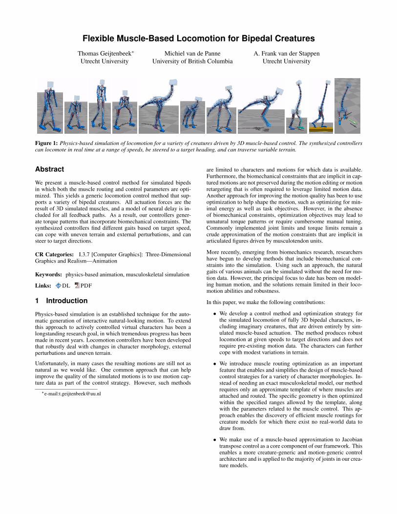
Figure 1: Physics-based simulation of locomotion for a variety of creatures driven by 3D muscle-based control. The synthesized controllerscan locomote in real time at a range of speeds, be steered to a target heading, and can traverse variable terrain.

Abstract

We present a muscle-based control method for simulated bipedsin which both the muscle routing and control parameters are opti-mized. This yields a generic locomotion control method that sup-ports a variety of bipedal creatures. All actuation forces are theresult of 3D simulated muscles, and a model of neural delay is in-cluded for all feedback paths. As a result, our controllers gener-ate torque patterns that incorporate biomechanical constraints. Thesynthesized controllers find different gaits based on target speed,can cope with uneven terrain and external perturbations, and cansteer to target directions.

CR Categories: I.3.7 [Computer Graphics]: Three-DimensionalGraphics and Realism—Animation

Keywords: physics-based animation, musculoskeletal simulation

Links: DL PDF

1 Introduction

Physics-based simulation is an established technique for the auto-matic generation of interactive natural-looking motion. To extendthis approach to actively controlled virtual characters has been alongstanding research goal, in which tremendous progress has beenmade in recent years. Locomotion controllers have been developedthat robustly deal with changes in character morphology, externalperturbations and uneven terrain.

Unfortunately, in many cases the resulting motions are still not asnatural as we would like. One common approach that can helpimprove the quality of the simulated motions is to use motion cap-ture data as part of the control strategy. However, such methods

∗e-mail:t.geijtenbeek@uu.nl

are limited to characters and motions for which data is available.Furthermore, the biomechanical constraints that are implicit in cap-tured motions are not preserved during the motion editing or motionretargeting that is often required to leverage limited motion data.Another approach for improving the motion quality has been to useoptimization to help shape the motion, such as optimizing for min-imal energy as well as task objectives. However, in the absenceof biomechanical constraints, optimization objectives may lead tounnatural torque patterns or require cumbersome manual tuning.Commonly implemented joint limits and torque limits remain acrude approximation of the motion constraints that are implicit inarticulated figures driven by musculotendon units.

More recently, emerging from biomechanics research, researchershave begun to develop methods that include biomechanical con-straints into the simulation. Using such an approach, the naturalgaits of various animals can be simulated without the need for mo-tion data. However, the principal focus to date has been on model-ing human motion, and the solutions remain limited in their loco-motion abilities and robustness.

In this paper, we make the following contributions:

• We develop a control method and optimization strategy forthe simulated locomotion of fully 3D bipedal characters, in-cluding imaginary creatures, that are driven entirely by sim-ulated muscle-based actuation. The method produces robustlocomotion at given speeds to target directions and does notrequire pre-existing motion data. The characters can furthercope with modest variations in terrain.

• We introduce muscle routing optimization as an importantfeature that enables and simplifies the design of muscle-basedcontrol strategies for a variety of character morphologies. In-stead of needing an exact musculoskeletal model, our methodrequires only an approximate template of where muscles areattached and routed. The specific geometry is then optimizedwithin the specified ranges allowed by the template, alongwith the parameters related to the muscle control. This ap-proach enables the discovery of efficient muscle routings forcreature models for which there exist no real-world data todraw from.

• We make use of a muscle-based approximation to Jacobiantranspose control as a core component of our framework. Thisenables a more creature-generic and motion-generic controlarchitecture and is applied to the majority of joints in our crea-ture models.

2 Related Work

Methods for physics-based character animation that use forwarddynamic simulations have been a research focus for over twodecades, most often with human locomotion as the motion of inter-est. A survey of the considerable body of work in this area can befound in [Geijtenbeek and Pronost 2012]. A rigid-link articulatedfigure is typically driven by treating the joint torques at each timestep as free variables, constrained by joint angle limits and jointtorque limits. The underlying balance strategies commonly makedirect or indirect use of foot placement, e.g., [Raibert and Hodgins1991; Hodgins et al. 1995; Laszlo et al. 1996; Yin et al. 2007; Tsaiet al. 2010]. Basic locomotion capabilities have been extended ina variety of ways, including coping with terrain variations, charac-ter morphology variations, flexibly parameterized walking and run-ning, new types of motions, new control abstractions, and methodsfor flexible motion sequencing. Examples here include [Faloutsoset al. 2001; Wang et al. 2009; Coros et al. 2009; Jain et al. 2009;Wang et al. 2010; Wu and Popovic 2010; Mordatch et al. 2010;de Lasa et al. 2010; Ye and Liu 2010; Coros et al. 2010; Jain andLiu 2011; Liu et al. 2012].

The use of motion capture data can greatly help in achieving naturalphysics-based locomotion. It can be used as a reference trajectory,as a well-chosen initialization point for an optimization, or as an ex-ample of an optimal solution from which to then generalize furthersolutions. A number of approaches exploit motion data to achievetorque-based control of simulated human motions [Liu et al. 2005;Sok et al. 2007; Yin et al. 2007; da Silva et al. 2008a; da Silvaet al. 2008b; Muico et al. 2009; Lee et al. 2010; Kwon and Hod-gins 2010; Jain and Liu 2011; Muico et al. 2011; Geijtenbeek et al.2012]. Many of these methods further tackle aspects of parameteri-zation, other classes of motion, and choice of feedback abstraction.

In reality, joint torques cannot be commanded at will and must in-stead arise from muscles that have their own activation dynamics,force production behavior, and moment arms that change over time.They also often do not provide direct control over individual de-grees of freedom, as is assumed with computed torque methods.This is because a single muscle may span multiple joints, and asingle joint may be spanned by multiple muscles. Biomechanicsresearch has developed muscle-based approaches for the simula-tion of a variety of human and animal motions, including lizards[Ijspeert et al. 2007], cat hind limbs [Maufroy et al. 2008], humanjumping [Pandy et al. 1992], human pedaling [Thelen et al. 2003],and human gait [Taga 1995; Anderson and Pandy 2001; Geyerand Herr 2010; Ackermann and van den Bogert 2012]. Relatedly,muscle-based simulations are being explored in the computer ani-mation literature, where they are applied to modeling human handmotion [Tsang et al. 2005; Sueda et al. 2008], human upper bodymotion [Lee et al. 2010], and to evaluating the realism of humanmotion trajectories [Geijtenbeek et al. 2010]. Most notably, thework of Geyer and Herr [2010] has been used as the basis to an-imate a full 3D humanoid character by Wang et al. [2012]. Themotion controls are optimized with respect to an objective functionthat combines metabolic energy consumption and several walking-task-specific terms related to head stability and torso orientation.Together with muscle reflex models, this then produces stable for-ward dynamics simulations of walking at a variety of speeds thatare shown to closely match human walking data.

While the majority of work on physics-based character simulationis focused on modeling human motion, control strategies have alsobeen developed to drive simulations of block-based creatures [Sims1994], swimming creatures [Grzeszczuk and Terzopoulos 1995;Tan et al. 2011], walking birds or other fantastical bipeds [Coroset al. 2009; Coros et al. 2010; de Lasa et al. 2010], and quadrupeds[Coros et al. 2011]. Physically-plausible gaits are developed de

novo, i.e., without motion capture data, by Wampler et al. [Wamplerand Popovic 2009; Wampler et al. 2013]. Alternate kinematic ap-proaches are developed by Hecker et al. [2008] and Kry et al.[2009] for producing visually plausible gaits for arbitrary creaturemorphologies.

Our work is most closely related to the impressive state-of-the-artwork by Wang et al. [2012]. We share many of the goals of thisrecent work, but with the following notable differences: (1) Themodels we develop use 3D muscles to drive all the motion of theentire body. In comparson, Wang et al. [2012] use planar mus-cles restricted to the sagittal-plane to control the lower body, anduse classic torque-based methods to control the coronal lower-bodymotion and the entire upper body. Our models are entirely muscledriven. (2) Our framework optimizes for the best muscle routinggeometry. As such, the user only needs to provide an approxi-mate template for muscle insertions and attachments. This is ofparticular utility when designing imaginary creatures or dispropor-tional humans, for which these parameters are not known. Properrouting of 3D muscles can greatly simplify control, and we showthat this aspect of the optimization significantly contributes to theability to synthesize plausible motions. (3) We optimize for mus-cle physiological properties, including rest length and maximumforce. These are not known a priori when designing new creatures.(4) Our control system relies heavily on target features (positionsand orientations of links), and uses a muscle-based Jacobian trans-pose approximation to help compute target muscle activations. Thiscontributes towards a more generic control framework. In contrast,the feedback rules of Wang et al. [2012] are tailored around thehuman-specific reflex model developed by Geyer and Herr [2010].(5) Our controllers are robust enough to traverse moderate terrainvariations and can perform shallow turns. (6) Most significantly,our method can be applied to automatically achieve different gaitsfor a variety of creatures, including imaginary creatures.

We note that the above differences are not always entirely ben-eficial. Because our framework targets a wider variety of crea-tures with a control architecture that attempts to be more genericrather than being tailored to human models, our basic approach maynot achieve the same human motion fidelity as the human-specificmethod and results presented by Wang et al. [2012]. However, re-searchers focusing on achieving a more faithful human gait (or anyother gait) can easily extend our basic approach by adding domain-specific target features, objective terms or feedback rules.

3 Musculoskeletal Model

Our creature model consists of a hierarchy of rigid bodies, whichare actuated using an established dynamic muscle model [Geyerand Herr 2010]. The biomechanical constraints incorporated in thismodel ensure the creation of realistic and smooth torque patterns.More specifically, it models the physiological properties of con-tractile muscle fibers and tendons (contraction dynamics), and theelectro-chemical process that leads to changes in activation state(activation dynamics).

3.1 Muscle Contraction Dynamics

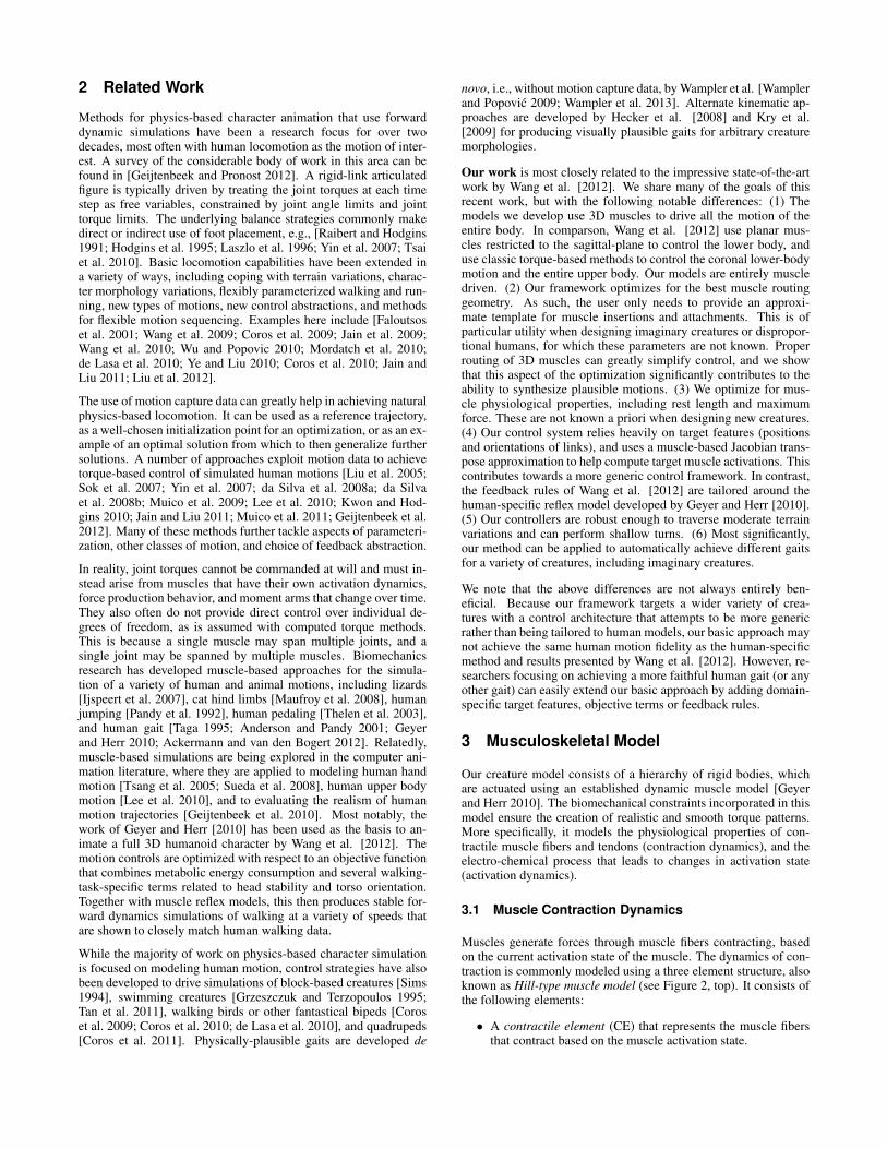
Muscles generate forces through muscle fibers contracting, basedon the current activation state of the muscle. The dynamics of con-traction is commonly modeled using a three element structure, alsoknown as Hill-type muscle model (see Figure 2, top). It consists ofthe following elements:

• A contractile element (CE) that represents the muscle fibersthat contract based on the muscle activation state.

PEESEE

CE

LCE LSEE

LM

0.0

0.5

1.0

0 1 2

Force-Length

0.0

0.5

1.0

1.5

-10 -5 0 5 10

Force-Velocity

Figure 2: Top: The three components of a Hill-type muscle. Bot-tom: Normalized force-length and force-velocity relations of thecontractile element.

• A parallel elastic element (PEE) that represents the passiveelastic material surrounding muscle fibers.

• A serial elastic element (SEE) that represents the tendons thatconnect the muscle to the bones.

The force produced by the CE, FCE, depends on the constant max-imum isometrical force for the muscle, Fmax, the muscle activationa, fiber length LCE, and contraction velocity VCE:

FCE = a Fmax fL(LCE) fV(VCE) (1)

where fL describes the relationship between force and length ofa muscle, and fV describes the relationship between force and thecurrent contraction velocity (see Figure 2, bottom). Roughly speak-ing, a muscle can produce more force when its length is closerto its optimal length, and produces less force if it is contractingfaster. The maximum isometric force Fmax is a constant that wefind through optimization.

The passive forces produced by the elastic elements, FPEE andFSEE are modeled as non-linear springs based on their length:

FSEE = fSEE(LM − LCE) (2)FPEE = fPEE(LCE) (3)

where fSEE and fPEE are non-linear force-length relations and LM

represents the total muscle length, from which the length of theSEE can be derived. Analytical forms of fSEE, fPEE, fL and fV

are described in [Geyer et al. 2003].

As the SEE is wired to the CE and PEE in series, the total muscleforce FM is subject to the force balance equation

FM = FCE + FPEE = FSEE (4)

The length of the CE (from which the SEE length is derived) isinitialized to be its optimal length, Lopt

CE , which in combination withthe tendon slack length Lslack

SEE defines the muscle rest length LrestM :

LrestM = Lslack

SEE + LoptCE (5)

Both LoptCE and Lslack

SEE are important for the dynamic behavior ofthe muscle [Zajac 1989] and are subject to optimization. Duringsimulation, activation state a and total muscle length LM are input

p1

p2

p4

p3

p1x

p1z

p2xp2y

p2zp4y

b1

b2b3

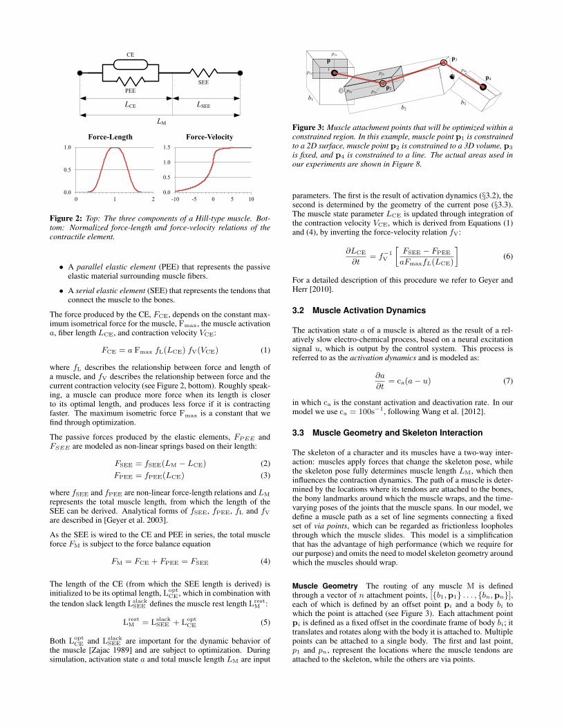
Figure 3: Muscle attachment points that will be optimized within aconstrained region. In this example, muscle point p1 is constrainedto a 2D surface, muscle point p2 is constrained to a 3D volume, p3

is fixed, and p4 is constrained to a line. The actual areas used inour experiments are shown in Figure 8.

parameters. The first is the result of activation dynamics (§3.2), thesecond is determined by the geometry of the current pose (§3.3).The muscle state parameter LCE is updated through integration ofthe contraction velocity VCE, which is derived from Equations (1)and (4), by inverting the force-velocity relation fV:

∂LCE

∂t= f−1

V

[FSEE − FPEE

aFmaxfL(LCE)

](6)

For a detailed description of this procedure we refer to Geyer andHerr [2010].

3.2 Muscle Activation Dynamics

The activation state a of a muscle is altered as the result of a rel-atively slow electro-chemical process, based on a neural excitationsignal u, which is output by the control system. This process isreferred to as the activation dynamics and is modeled as:

∂a

∂t= ca(a− u) (7)

in which ca is the constant activation and deactivation rate. In ourmodel we use ca = 100s−1, following Wang et al. [2012].

3.3 Muscle Geometry and Skeleton Interaction

The skeleton of a character and its muscles have a two-way inter-action: muscles apply forces that change the skeleton pose, whilethe skeleton pose fully determines muscle length LM, which theninfluences the contraction dynamics. The path of a muscle is deter-mined by the locations where its tendons are attached to the bones,the bony landmarks around which the muscle wraps, and the time-varying poses of the joints that the muscle spans. In our model, wedefine a muscle path as a set of line segments connecting a fixedset of via points, which can be regarded as frictionless loopholesthrough which the muscle slides. This model is a simplificationthat has the advantage of high performance (which we require forour purpose) and omits the need to model skeleton geometry aroundwhich the muscles should wrap.

Muscle Geometry The routing of any muscle M is definedthrough a vector of n attachment points, [{b1,p1} . . . , {bn,pn}],each of which is defined by an offset point pi and a body bi towhich the point is attached (see Figure 3). Each attachment pointpi is defined as a fixed offset in the coordinate frame of body bi; ittranslates and rotates along with the body it is attached to. Multiplepoints can be attached to a single body. The first and last point,p1 and pn, represent the locations where the muscle tendons areattached to the skeleton, while the others are via points.

p1

j2

j1

s1

FM

p2

s2

p4

s3F

M

p3

τ1

τ2

r1 r2

Figure 4: Example muscle path with four attachment points, threebodies and two joints.

The total muscle length LM is equal to the summed lengths of then− 1 muscle segments, [s1, . . . , sn−1], which are found using theposition of each point in the world coordinate frame, pW

i :

LM =

n−1∑i=1

‖si‖ , si = pWi+1 − pW

i (8)

The location of these attachment points has a great influence onboth direction and magnitude of the torque a muscle can produce.The direction of the moment arm (and thereby its function) changesdynamically with the character pose; this relation is fully based onthe locations of the attachment points. The amount of torque a mus-cle can provide depends on the projected distance between a mus-cle segment and the joint it spans. If it is further away, the momentarm is higher, but joint rotations will also lead to bigger changesin length, which limits the range in which the muscle can operate.Both aspects greatly affect control.

In our approach, we attempt to find efficient muscle routingsthrough optimization. We do so by defining an area Pi in whicha muscle point pi must be contained. In our implementation, we al-low variation of selected Cartesian components px, py or py withina range that is specified in an attachment template. Depending onthe number of free components, the point pi is either fixed, or con-strained to a line, a plane or a box (see Figure 3).

Force Application The total muscle length LM is used in com-bination with the activation state a to compute the (scalar) musclecontraction force FM. This force is transmitted to the skeleton ateach attachment point to the body it is attached to, and generates atorque over each joint it spans. For each joint k, a torque τk is gen-erated in the direction defined by moment arm rk. This momentarm corresponds to the cross-product between the direction of themuscle segment that crosses the joint, sc, and a vector from jointcenter jk to any point on segment sc (e.g. point pW

c ):

τk = FM‖rk‖ , rk = (pWc − jk)× sc

‖sc‖(9)

The direction and size of moment arm rk change as a function ofthe character pose, based on the geometry of sc (see Figure 4).

4 Control

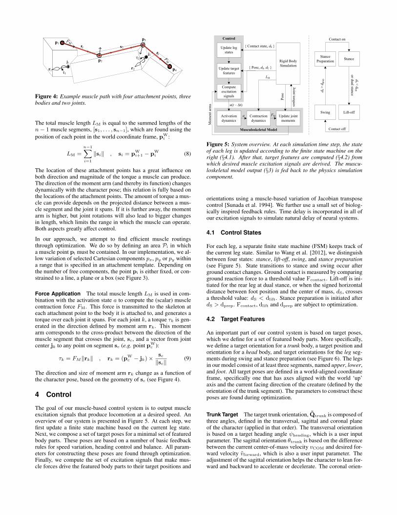
The goal of our muscle-based control system is to output muscleexcitation signals that produce locomotion at a desired speed. Anoverview of our system is presented in Figure 5. At each step, wefirst update a finite state machine based on the current leg state.Next, we compose a set of target poses for a minimal set of featuredbody parts. These poses are based on a number of basic feedbackrules for speed variation, heading control and balance. All param-eters for constructing these poses are found through optimization.Finally, we compute the set of excitation signals that make mus-cle forces drive the featured body parts to their target positions and

Control

Musculoskeletal Model

Update leg states

Compute excitation

signals

Activation dynamics

Update target features

Contraction dynamics

Rigid Body Simulation

{ Contact state, dS }

{ Pose, dS, dC }

Pose

a

u(t – Δt)

Update joint moments

FM

Mom

ent a

rms

Stance

Swing Lift-off

Stance Preparation

dS < d

liftor dual stance

Contact off

d S >

dpr

ep

Contact on

Joint torques

LM

Figure 5: System overview. At each simulation time step, the stateof each leg is updated according to the finite state machine on theright (§4.1). After that, target features are computed (§4.2) fromwhich desired muscle excitation signals are derived. The muscu-loskeletal model output (§3) is fed back to the physics simulationcomponent.

orientations using a muscle-based variation of Jacobian transposecontrol [Sunada et al. 1994]. We further use a small set of biolog-ically inspired feedback rules. Time delay is incorporated in all ofour excitation signals to simulate natural delay of neural systems.

4.1 Control States

For each leg, a separate finite state machine (FSM) keeps track ofthe current leg state. Similar to Wang et al. [2012], we distinguishbetween four states: stance, lift-off, swing, and stance preparation(see Figure 5). State transitions to stance and swing occur afterground contact changes. Ground contact is measured by comparingground reaction force to a threshold value Fcontact. Lift-off is ini-tiated for the rear leg at dual stance, or when the signed horizontaldistance between foot position and the center of mass, dS, crossesa threshold value: dS < dlift. Stance preparation is initiated afterdS > dprep. Fcontact, dlift and dprep are subject to optimization.

4.2 Target Features

An important part of our control system is based on target poses,which we define for a set of featured body parts. More specifically,we define a target orientation for a trunk body, a target position andorientation for a head body, and target orientations for the leg seg-ments during swing and stance preparation (see Figure 6). The legsin our model consist of at least three segments, named upper, lower,and foot. All target poses are defined in a world-aligned coordinateframe, specifically one that has axes aligned with the world ‘up’axis and the current facing direction of the creature (defined by theorientation of the trunk segment). The parameters to construct theseposes are found during optimization.

Trunk Target The target trunk orientation, Qtrunk is composed ofthree angles, defined in the transversal, sagittal and coronal planeof the character (applied in that order). The transversal orientationis based on a target heading angle ψheading, which is a user inputparameter. The sagittal orientation θtrunk is based on the differencebetween the current center-of-mass velocity vCOM and desired for-ward velocity vforward, which is also a user input parameter. Theadjustment of the sagittal orientation helps the character to lean for-ward and backward to accelerate or decelerate. The coronal orien-

Trun

k

Head

Foot

Lower

UpperθH

θK

θF

θT φT ψheading

Phead Phead

Phead

dC

CoronalSagittal Transversal

dS

φH

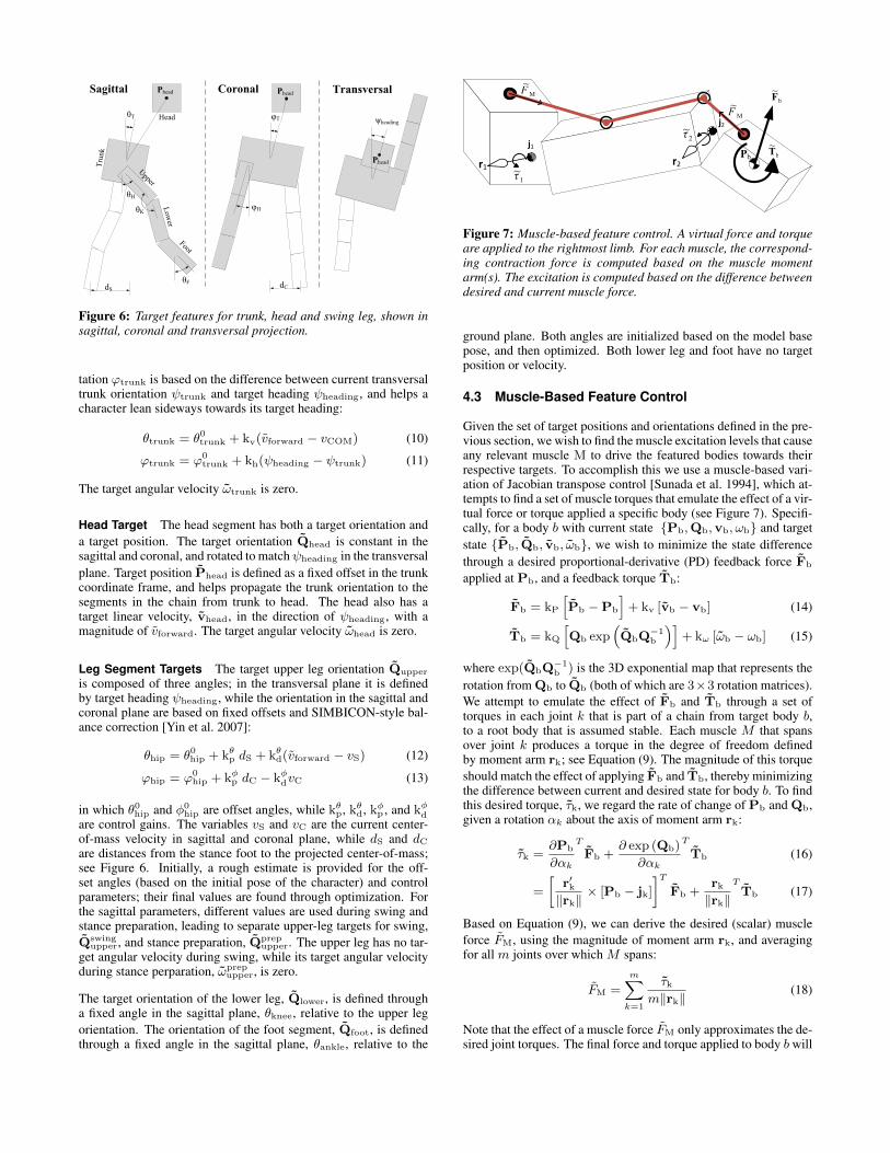
Figure 6: Target features for trunk, head and swing leg, shown insagittal, coronal and transversal projection.

tation ϕtrunk is based on the difference between current transversaltrunk orientation ψtrunk and target heading ψheading, and helps acharacter lean sideways towards its target heading:

θtrunk = θ0trunk + kv(vforward − vCOM) (10)

ϕtrunk = ϕ0trunk + kh(ψheading − ψtrunk) (11)

The target angular velocity ωtrunk is zero.

Head Target The head segment has both a target orientation anda target position. The target orientation Qhead is constant in thesagittal and coronal, and rotated to matchψheading in the transversalplane. Target position Phead is defined as a fixed offset in the trunkcoordinate frame, and helps propagate the trunk orientation to thesegments in the chain from trunk to head. The head also has atarget linear velocity, vhead, in the direction of ψheading, with amagnitude of vforward. The target angular velocity ωhead is zero.

Leg Segment Targets The target upper leg orientation Qupper

is composed of three angles; in the transversal plane it is definedby target heading ψheading, while the orientation in the sagittal andcoronal plane are based on fixed offsets and SIMBICON-style bal-ance correction [Yin et al. 2007]:

θhip = θ0hip + kθp dS + kθd(vforward − vS) (12)

ϕhip = ϕ0hip + kφp dC − kφdvC (13)

in which θ0hip and φ0

hip are offset angles, while kθp, kθd, kφp , and kφdare control gains. The variables vS and vC are the current center-of-mass velocity in sagittal and coronal plane, while dS and dC

are distances from the stance foot to the projected center-of-mass;see Figure 6. Initially, a rough estimate is provided for the off-set angles (based on the initial pose of the character) and controlparameters; their final values are found through optimization. Forthe sagittal parameters, different values are used during swing andstance preparation, leading to separate upper-leg targets for swing,Qswing

upper, and stance preparation, Qprepupper. The upper leg has no tar-

get angular velocity during swing, while its target angular velocityduring stance perparation, ωprep

upper, is zero.

The target orientation of the lower leg, Qlower, is defined througha fixed angle in the sagittal plane, θknee, relative to the upper legorientation. The orientation of the foot segment, Qfoot, is definedthrough a fixed angle in the sagittal plane, θankle, relative to the

j2

j1

r1 r2Pb b

~T

M~F

b~FM

~F

1~τ

2~τ

Figure 7: Muscle-based feature control. A virtual force and torqueare applied to the rightmost limb. For each muscle, the correspond-ing contraction force is computed based on the muscle momentarm(s). The excitation is computed based on the difference betweendesired and current muscle force.

ground plane. Both angles are initialized based on the model basepose, and then optimized. Both lower leg and foot have no targetposition or velocity.

4.3 Muscle-Based Feature Control

Given the set of target positions and orientations defined in the pre-vious section, we wish to find the muscle excitation levels that causeany relevant muscle M to drive the featured bodies towards theirrespective targets. To accomplish this we use a muscle-based vari-ation of Jacobian transpose control [Sunada et al. 1994], which at-tempts to find a set of muscle torques that emulate the effect of a vir-tual force or torque applied a specific body (see Figure 7). Specifi-cally, for a body b with current state {Pb,Qb,vb, ωb} and targetstate {Pb, Qb, vb, ωb}, we wish to minimize the state differencethrough a desired proportional-derivative (PD) feedback force Fb

applied at Pb, and a feedback torque Tb:

Fb = kP

[Pb −Pb

]+ kv [vb − vb] (14)

Tb = kQ

[Qb exp

(QbQ

−1b

)]+ kω [ωb − ωb] (15)

where exp(QbQ−1b ) is the 3D exponential map that represents the

rotation from Qb to Qb (both of which are 3×3 rotation matrices).We attempt to emulate the effect of Fb and Tb through a set oftorques in each joint k that is part of a chain from target body b,to a root body that is assumed stable. Each muscle M that spansover joint k produces a torque in the degree of freedom definedby moment arm rk; see Equation (9). The magnitude of this torqueshould match the effect of applying Fb and Tb, thereby minimizingthe difference between current and desired state for body b. To findthis desired torque, τk, we regard the rate of change of Pb and Qb,given a rotation αk about the axis of moment arm rk:

τk =∂Pb

∂αk

T

Fb +∂ exp (Qb)

∂αk

T

Tb (16)

=

[r′k‖rk‖

× [Pb − jk]

]TFb +

rk

‖rk‖TTb (17)

Based on Equation (9), we can derive the desired (scalar) muscleforce FM, using the magnitude of moment arm rk, and averagingfor all m joints over which M spans:

FM =

m∑k=1

τkm‖rk‖

(18)

Note that the effect of a muscle force FM only approximates the de-sired joint torques. The final force and torque applied to body b will

in practice deviate from Fb and Tb, and depend on the geometryand state of the individual muscles included in the chain of bodies,as well as the stability of the root body. However, we found thisapproximation to work well in practice, especially since the gainsfor Fb and Tb are subject to optimization.

The desired activation level aM is estimated based on the maximumisometric force Fmax:

aM =FM

Fmax(19)

In this estimation, we ignore the current length and velocity thatare part of Equation (1). We have found that including length andvelocity relations into our approximate inverse model for the con-traction dynamics causes oscillations in muscle activation, becauselength and velocity change significantly over the course of neuraland activation delay.

4.4 Muscle Activations

To compute the muscle excitation levels for our control system, weuse a combination of muscle-based feature control, positive force-feedback [Geyer et al. 2006], and constant excitation values. Weomit the use of length-based feedback rules defined in Geyer andHerr [2010] and Wang et al. [2012] in favor of our muscle-basedfeature control. A time delay is added to all feedback paths to sim-ulate neural delay. For each muscle M involved in muscle-basedfeature control, we set the output excitation to match the desiredactivation:

uM = aMt−∆t (20)

in which t−∆t represents the application of a delay ∆t. FollowingGeyer and Herr [2010], we use ∆t = 20ms for muscles attachedto the foot, ∆t = 10ms for muscles attached to lower leg, and∆t = 5ms for muscles attached to upper leg. For other muscles, weuse ∆t = 5ms. Alternatively, the amount of delay could directlybe derived from the distance of the muscle to the brain.

Trunk Orientation Feedback During stance, the orientation ofthe trunk is stabilized and rotated towards its target orientationQtrunk by all muscles connecting the trunk segment to a stanceleg segment. The excitation for each HIP muscle corresponds to:

ustanceHIP = aHIP(Qtrunk, ωtrunk)

t−∆t(21)

Note that this feedback performs a rotation in 3 dimensions, de-pending on the planes in which the muscles operate.

Head Position and Orientation Feedback The head is movedtowards its target state by all muscles connected to any body in thechain from trunk to head. The excitation is defined as:

uS = aS(Qhead, ωhead, Phead, vhead)t−∆t

(22)

Stance and Lift-Off Feedback For the stance leg, we do not de-fine target orientations or positions. Instead, we rely on positiveforce feedback to achieve natural joint compliance [Geyer et al.2006]:

uF+ = kF+M FM

t−∆t(23)

in which kF+M is a constant feedback gain found during optimiza-

tion. The length-force and velocity-force relations of any muscleensure the excitation level does not increase indefinitely. Positive

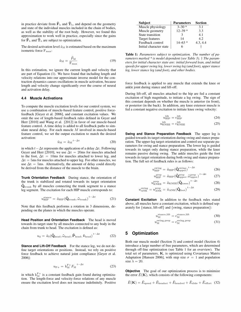
Subject Parameters SectionMuscle physiology 3–30 * 3.1Muscle geometry 12–39 * 3.3State transition 3 4.1Target features 14 4.2Feedback control 14–63 * 4.3, 4.4Initial character state 6 †

Table 1: Parameters subject to optimization. The number of pa-rameters marked * is model dependent (see Table 3). † The param-eters for initial character state are: initial forward lean, and initialspeeds for upper swing leg, lower swing leg (and foot), upper stanceleg, lower stance leg (and foot), and other bodies.

force feedback is applied to any muscle that extends the knee orankle joint during stance and lift-off.

During lift-off, all muscles attached to the hip are fed a constantexcitation of high magnitude, to initiate a leg swing. The sign ofthis constant depends on whether the muscle is anterior (in front),or posterior (in the back). In addition, any knee extensor muscle isfed a constant negative excitation to initiate knee swing velocity:

uliftHIP = clift

HIP (24)

uliftKNEE = clift

KNEE (25)

Swing and Stance Preparation Feedback The upper leg isguided towards its target orientation during swing and stance prepa-ration. The upper-leg target orientation and control use separate pa-rameters for swing and stance preparation. The lower leg is guidedtowards its target only during stance preparation, while the kneeremains passive during swing. The ankle muscles guide the foottowards its target orientation during both swing and stance prepara-tion. The full set of feedback rules is as follows:

uswingHIP = aHIP(Qswing

upper)t−∆t

(26)

uprepHIP = aHIP(Qprep

upper, ωprepupper)

t−∆t(27)

uprepKNEE = aKNEE(Qlower)

t−∆t(28)

uswingANK = uprep

ANK = aANK(Qfoot)t−∆t

(29)

Constant Excitation In addition to the feedback rules statedabove, all muscles have a constant excitation, which is defined sep-arately for {stance, lift-off} and {swing, stance preparation}:

ustance,liftM = cstance,lift

M (30)

uswing,prepM = cswing,prep

M (31)

5 Optimization

Both our muscle model (Section 3) and control model (Section 4)introduce a large number of free parameters, which are determinedthrough off-line optimization (see Table 1 for an overview). Thetotal set of parameters, K, is optimized using Covariance MatrixAdaptation [Hansen 2006], with step size σ = 1 and populationsize λ = 20.

Objective The goal of our optimization process is to minimizethe error E(K), which consists of the following components:

E(K) = Espeed + Eheadori + Eheadvel + Eslide + Eeffort (32)

Evelspeed Eori

head Evelhead Eslide Eeffort

Weight (Wm) 100 10 10 10 0.1Treshold (Hm) 0.1 0.2 0.3 0.2 0

Table 2: Weights and thresholds for the individual error measures.

Each right hand term is acquired by integrating a time dependentmeasure Em(t) over a specific duration tmax:

Em = Wm

{∫ tmax

0

Em(t) ∂t

}Hm

(33)

in which Wm is measure-specific weight, while {}Hm enforces ameasure-specific threshold: the value between braces is set to zeroif it is lower than Hm. This allows for a prioritized optimization, asheavily weighted terms have greater influence until they reach theirthreshold. A significant difference with the error measure of Wanget al. [2012] is that we apply this threshold after integration, allow-ing incidental high values to be compensated by below-thresholdaverages. This is especially relevant for the initial stage of the sim-ulation, when a character is still finding its pace. The individualweights and thresholds for each of the error terms are shown in Ta-ble 2.

The measure for target speed, Espeed(t), is computed as thenormalized difference between base speed and target velocityvforward(t):

Espeed(t) = ‖1− vbase(t)

vforward(t)‖ (34)

in which vbase(t) is the forward speed based on the average footposition, updated at each contact initiation. To increase head sta-bility, we use an error measure Eheadori(t) for deviation of headorientation from its target, and Eheadvel(t) for deviation for linearhead velocity from its target:

Eheadori(t) = ‖Q−1head(t)Qhead(t)‖ (35)

Eheadvel(t) = ‖vhead − vhead(t)‖ (36)

In some of our simulations, we experienced a local minimum asthe result of foot sliding. Error measure Eslide(t) prevents this bypenalizing through average contact velocity vcontact(t):

Eslide(t) = vcontact(t) (37)

For effort minimization Eeffort(t), we use the current rate ofmetabolic expenditure [Wang et al. 2012].

Termination Conditions During the evaluation ofE(K), we ter-minate a simulation prematurely when failure is detected to save onsimulation time and to help prevent local minima in the optimiza-tion. The following tests are performed during each time step:

• Center-of-Mass Height. To detect falling, we measure thecenter-of-mass position and compare its height to the initialstate. The simulation is terminated if the measured height fallsbelow a certain threshold. We use a factor of 0.9.

• Heading. We compare the target heading ψheading to the cur-rent trunk heading ψtrunk, and terminate if they deviate over45 degrees. In addition to keeping the character from drifting,this helps avoid a local minimum scenario where a characterthrusts its feet forward during a backwards turn.

• Self-Collision and Leg-Crossing. We terminate on both self-collision and leg crossing, to avoid local minima where a char-acter is unable to take another step because of self-collision.

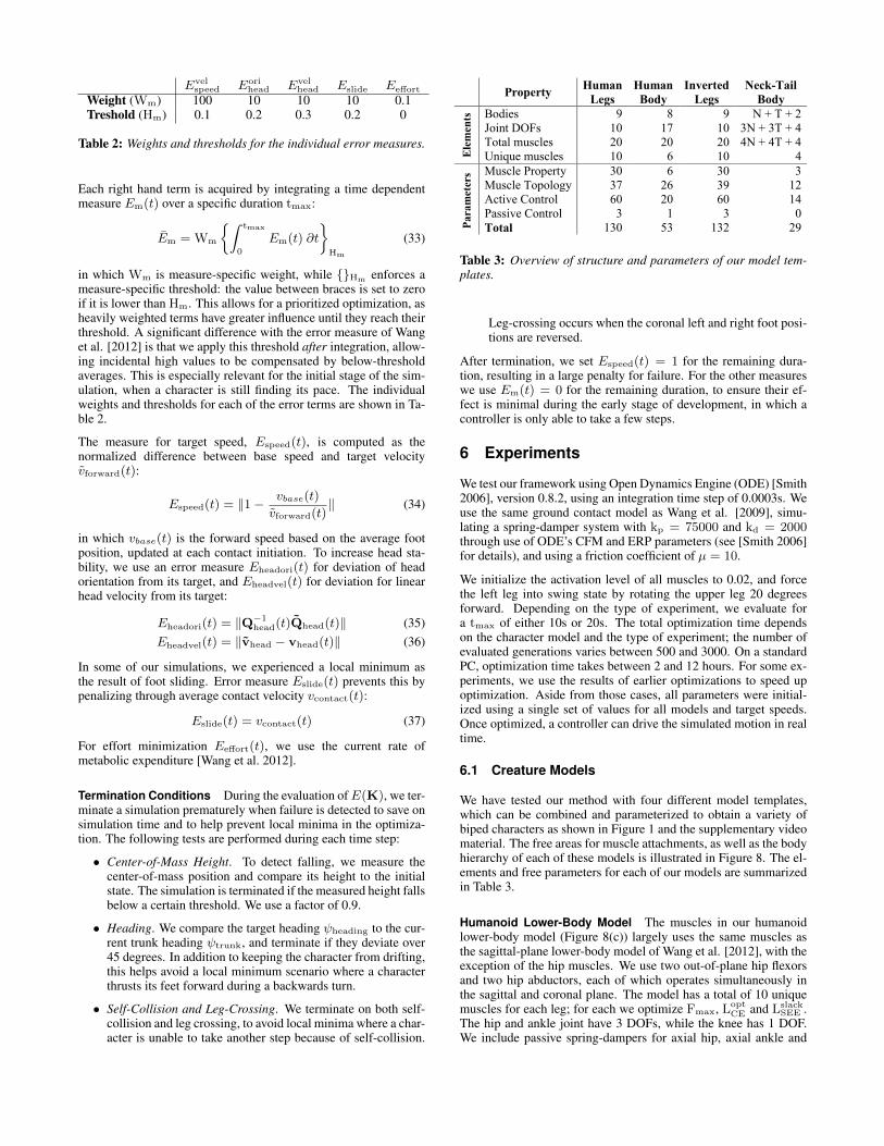
Property Human Legs

Human Body

Inverted Legs

Neck-Tail Body

Ele

men

ts Bodies 9 8 9 N + T + 2

Joint DOFs 10 17 10 3N + 3T + 4 Total muscles 20 20 20 4N + 4T + 4 Unique muscles 10 6 10 4

Para

met

ers Muscle Property 30 6 30 3

Muscle Topology 37 26 39 12 Active Control 60 20 60 14 Passive Control 3 1 3 0 Total 130 53 132 29

Table 3: Overview of structure and parameters of our model tem-plates.

Leg-crossing occurs when the coronal left and right foot posi-tions are reversed.

After termination, we set Espeed(t) = 1 for the remaining dura-tion, resulting in a large penalty for failure. For the other measureswe use Em(t) = 0 for the remaining duration, to ensure their ef-fect is minimal during the early stage of development, in which acontroller is only able to take a few steps.

6 Experiments

We test our framework using Open Dynamics Engine (ODE) [Smith2006], version 0.8.2, using an integration time step of 0.0003s. Weuse the same ground contact model as Wang et al. [2009], simu-lating a spring-damper system with kp = 75000 and kd = 2000through use of ODE’s CFM and ERP parameters (see [Smith 2006]for details), and using a friction coefficient of µ = 10.

We initialize the activation level of all muscles to 0.02, and forcethe left leg into swing state by rotating the upper leg 20 degreesforward. Depending on the type of experiment, we evaluate fora tmax of either 10s or 20s. The total optimization time dependson the character model and the type of experiment; the number ofevaluated generations varies between 500 and 3000. On a standardPC, optimization time takes between 2 and 12 hours. For some ex-periments, we use the results of earlier optimizations to speed upoptimization. Aside from those cases, all parameters were initial-ized using a single set of values for all models and target speeds.Once optimized, a controller can drive the simulated motion in realtime.

6.1 Creature Models

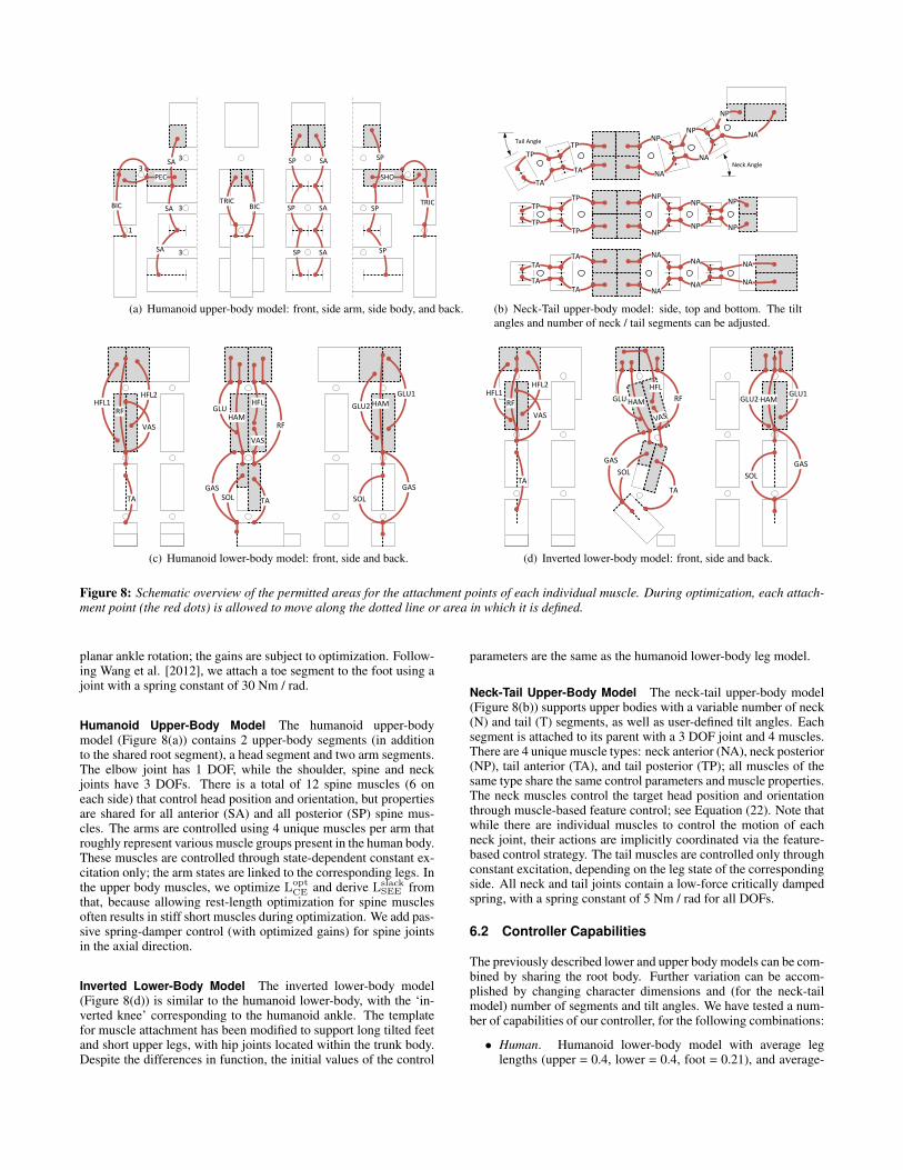
We have tested our method with four different model templates,which can be combined and parameterized to obtain a variety ofbiped characters as shown in Figure 1 and the supplementary videomaterial. The free areas for muscle attachments, as well as the bodyhierarchy of each of these models is illustrated in Figure 8. The el-ements and free parameters for each of our models are summarizedin Table 3.

Humanoid Lower-Body Model The muscles in our humanoidlower-body model (Figure 8(c)) largely uses the same muscles asthe sagittal-plane lower-body model of Wang et al. [2012], with theexception of the hip muscles. We use two out-of-plane hip flexorsand two hip abductors, each of which operates simultaneously inthe sagittal and coronal plane. The model has a total of 10 uniquemuscles for each leg; for each we optimize Fmax, Lopt

CE and LslackSEE .

The hip and ankle joint have 3 DOFs, while the knee has 1 DOF.We include passive spring-dampers for axial hip, axial ankle and

SA

PEC

SA

SATRIC

BIC

SA

SA

SASP

SP

SP SP

SP

SPBIC TRIC

SHO

3

3

3

3

1

(a) Humanoid upper-body model: front, side arm, side body, and back.

NP

TP

TA

TP

TANA

NA

NP

NA

NPNP

TPTP

NP

NP

NANA

TATA NA

Neck Angle

Tail Angle

NPNP

TPTP

NP

NANA

TATA NA

(b) Neck-Tail upper-body model: side, top and bottom. The tiltangles and number of neck / tail segments can be adjusted.

HFL

RF

GLU

VAS

GASSOL

HAM

HFL1HFL2

VAS

RF

TA

GLU2

GLU1HAM

GAS

SOLTA

(c) Humanoid lower-body model: front, side and back.

VAS

HFL

RFGLU

GAS

SOL

HAMHFL1

HFL2

VAS

RF

TA

GLU2GLU1

HAM

GAS

SOL

TA

(d) Inverted lower-body model: front, side and back.

Figure 8: Schematic overview of the permitted areas for the attachment points of each individual muscle. During optimization, each attach-ment point (the red dots) is allowed to move along the dotted line or area in which it is defined.

planar ankle rotation; the gains are subject to optimization. Follow-ing Wang et al. [2012], we attach a toe segment to the foot using ajoint with a spring constant of 30 Nm / rad.

Humanoid Upper-Body Model The humanoid upper-bodymodel (Figure 8(a)) contains 2 upper-body segments (in additionto the shared root segment), a head segment and two arm segments.The elbow joint has 1 DOF, while the shoulder, spine and neckjoints have 3 DOFs. There is a total of 12 spine muscles (6 oneach side) that control head position and orientation, but propertiesare shared for all anterior (SA) and all posterior (SP) spine mus-cles. The arms are controlled using 4 unique muscles per arm thatroughly represent various muscle groups present in the human body.These muscles are controlled through state-dependent constant ex-citation only; the arm states are linked to the corresponding legs. Inthe upper body muscles, we optimize Lopt

CE and derive LslackSEE from

that, because allowing rest-length optimization for spine musclesoften results in stiff short muscles during optimization. We add pas-sive spring-damper control (with optimized gains) for spine jointsin the axial direction.

Inverted Lower-Body Model The inverted lower-body model(Figure 8(d)) is similar to the humanoid lower-body, with the ‘in-verted knee’ corresponding to the humanoid ankle. The templatefor muscle attachment has been modified to support long tilted feetand short upper legs, with hip joints located within the trunk body.Despite the differences in function, the initial values of the control

parameters are the same as the humanoid lower-body leg model.

Neck-Tail Upper-Body Model The neck-tail upper-body model(Figure 8(b)) supports upper bodies with a variable number of neck(N) and tail (T) segments, as well as user-defined tilt angles. Eachsegment is attached to its parent with a 3 DOF joint and 4 muscles.There are 4 unique muscle types: neck anterior (NA), neck posterior(NP), tail anterior (TA), and tail posterior (TP); all muscles of thesame type share the same control parameters and muscle properties.The neck muscles control the target head position and orientationthrough muscle-based feature control; see Equation (22). Note thatwhile there are individual muscles to control the motion of eachneck joint, their actions are implicitly coordinated via the feature-based control strategy. The tail muscles are controlled only throughconstant excitation, depending on the leg state of the correspondingside. All neck and tail joints contain a low-force critically dampedspring, with a spring constant of 5 Nm / rad for all DOFs.

6.2 Controller Capabilities

The previously described lower and upper body models can be com-bined by sharing the root body. Further variation can be accom-plished by changing character dimensions and (for the neck-tailmodel) number of segments and tilt angles. We have tested a num-ber of capabilities of our controller, for the following combinations:

• Human. Humanoid lower-body model with average leglengths (upper = 0.4, lower = 0.4, foot = 0.21), and average-

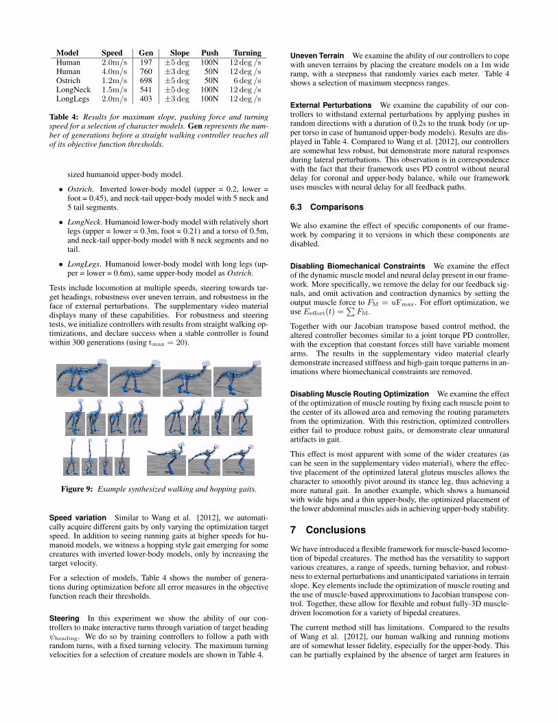
Model Speed Gen Slope Push TurningHuman 2.0m/s 197 ±5 deg 100N 12 deg /sHuman 4.0m/s 760 ±3 deg 50N 12 deg /sOstrich 1.2m/s 698 ±5 deg 50N 6 deg /sLongNeck 1.5m/s 541 ±5 deg 100N 12 deg /sLongLegs 2.0m/s 403 ±3 deg 100N 12 deg /s

Table 4: Results for maximum slope, pushing force and turningspeed for a selection of character models. Gen represents the num-ber of generations before a straight walking controller reaches allof its objective function thresholds.

sized humanoid upper-body model.

• Ostrich. Inverted lower-body model (upper = 0.2, lower =foot = 0.45), and neck-tail upper-body model with 5 neck and5 tail segments.

• LongNeck. Humanoid lower-body model with relatively shortlegs (upper = lower = 0.3m, foot = 0.21) and a torso of 0.5m,and neck-tail upper-body model with 8 neck segments and notail.

• LongLegs. Humanoid lower-body model with long legs (up-per = lower = 0.6m), same upper-body model as Ostrich.

Tests include locomotion at multiple speeds, steering towards tar-get headings, robustness over uneven terrain, and robustness in theface of external perturbations. The supplementary video materialdisplays many of these capabilities. For robustness and steeringtests, we initialize controllers with results from straight walking op-timizations, and declare success when a stable controller is foundwithin 300 generations (using tmax = 20).

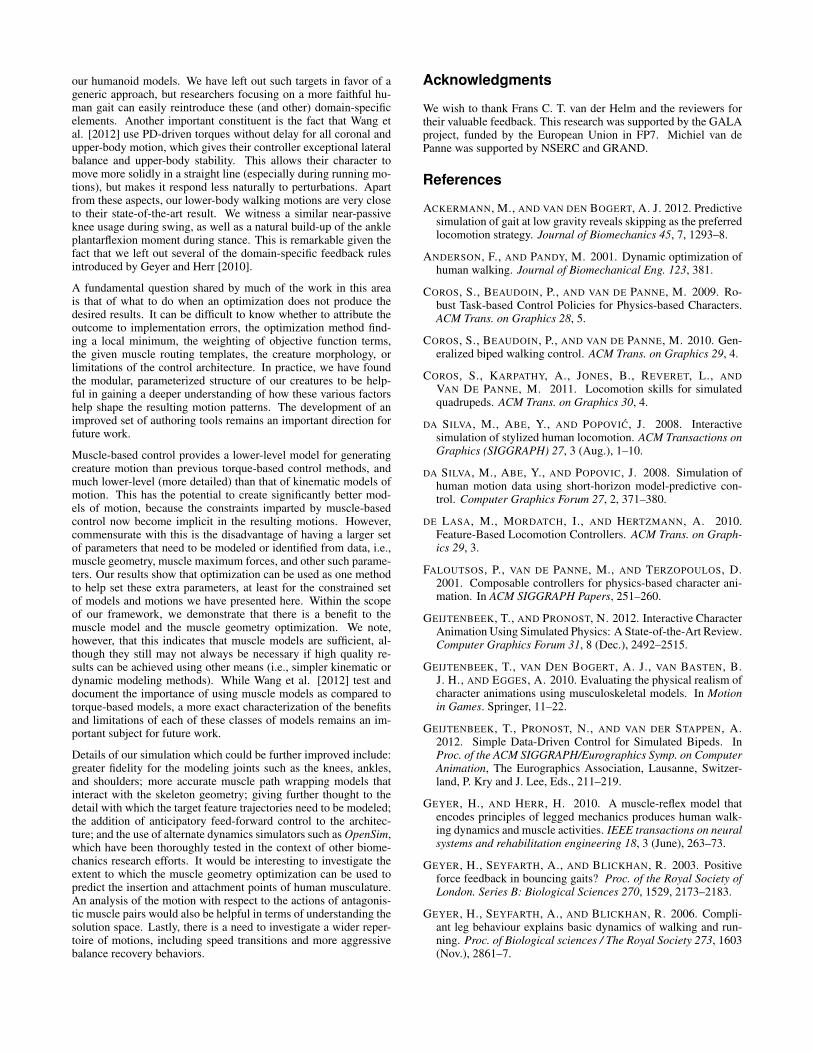
Figure 9: Example synthesized walking and hopping gaits.

Speed variation Similar to Wang et al. [2012], we automati-cally acquire different gaits by only varying the optimization targetspeed. In addition to seeing running gaits at higher speeds for hu-manoid models, we witness a hopping style gait emerging for somecreatures with inverted lower-body models, only by increasing thetarget velocity.

For a selection of models, Table 4 shows the number of genera-tions during optimization before all error measures in the objectivefunction reach their thresholds.

Steering In this experiment we show the ability of our con-trollers to make interactive turns through variation of target headingψheading. We do so by training controllers to follow a path withrandom turns, with a fixed turning velocity. The maximum turningvelocities for a selection of creature models are shown in Table 4.

Uneven Terrain We examine the ability of our controllers to copewith uneven terrains by placing the creature models on a 1m wideramp, with a steepness that randomly varies each meter. Table 4shows a selection of maximum steepness ranges.

External Perturbations We examine the capability of our con-trollers to withstand external perturbations by applying pushes inrandom directions with a duration of 0.2s to the trunk body (or up-per torso in case of humanoid upper-body models). Results are dis-played in Table 4. Compared to Wang et al. [2012], our controllersare somewhat less robust, but demonstrate more natural responsesduring lateral perturbations. This observation is in correspondencewith the fact that their framework uses PD control without neuraldelay for coronal and upper-body balance, while our frameworkuses muscles with neural delay for all feedback paths.

6.3 Comparisons

We also examine the effect of specific components of our frame-work by comparing it to versions in which these components aredisabled.

Disabling Biomechanical Constraints We examine the effectof the dynamic muscle model and neural delay present in our frame-work. More specifically, we remove the delay for our feedback sig-nals, and omit activation and contraction dynamics by setting theoutput muscle force to FM = uFmax. For effort optimization, weuse Eeffort(t) =

∑FM.

Together with our Jacobian transpose based control method, thealtered controller becomes similar to a joint torque PD controller,with the exception that constant forces still have variable momentarms. The results in the supplementary video material clearlydemonstrate increased stiffness and high-gain torque patterns in an-imations where biomechanical constraints are removed.

Disabling Muscle Routing Optimization We examine the effectof the optimization of muscle routing by fixing each muscle point tothe center of its allowed area and removing the routing parametersfrom the optimization. With this restriction, optimized controllerseither fail to produce robust gaits, or demonstrate clear unnaturalartifacts in gait.

This effect is most apparent with some of the wider creatures (ascan be seen in the supplementary video material), where the effec-tive placement of the optimized lateral gluteus muscles allows thecharacter to smoothly pivot around its stance leg, thus achieving amore natural gait. In another example, which shows a humanoidwith wide hips and a thin upper-body, the optimized placement ofthe lower abdominal muscles aids in achieving upper-body stability.

7 Conclusions

We have introduced a flexible framework for muscle-based locomo-tion of bipedal creatures. The method has the versatility to supportvarious creatures, a range of speeds, turning behavior, and robust-ness to external perturbations and unanticipated variations in terrainslope. Key elements include the optimization of muscle routing andthe use of muscle-based approximations to Jacobian transpose con-trol. Together, these allow for flexible and robust fully-3D muscle-driven locomotion for a variety of bipedal creatures.

The current method still has limitations. Compared to the resultsof Wang et al. [2012], our human walking and running motionsare of somewhat lesser fidelity, especially for the upper-body. Thiscan be partially explained by the absence of target arm features in

our humanoid models. We have left out such targets in favor of ageneric approach, but researchers focusing on a more faithful hu-man gait can easily reintroduce these (and other) domain-specificelements. Another important constituent is the fact that Wang etal. [2012] use PD-driven torques without delay for all coronal andupper-body motion, which gives their controller exceptional lateralbalance and upper-body stability. This allows their character tomove more solidly in a straight line (especially during running mo-tions), but makes it respond less naturally to perturbations. Apartfrom these aspects, our lower-body walking motions are very closeto their state-of-the-art result. We witness a similar near-passiveknee usage during swing, as well as a natural build-up of the ankleplantarflexion moment during stance. This is remarkable given thefact that we left out several of the domain-specific feedback rulesintroduced by Geyer and Herr [2010].

A fundamental question shared by much of the work in this areais that of what to do when an optimization does not produce thedesired results. It can be difficult to know whether to attribute theoutcome to implementation errors, the optimization method find-ing a local minimum, the weighting of objective function terms,the given muscle routing templates, the creature morphology, orlimitations of the control architecture. In practice, we have foundthe modular, parameterized structure of our creatures to be help-ful in gaining a deeper understanding of how these various factorshelp shape the resulting motion patterns. The development of animproved set of authoring tools remains an important direction forfuture work.

Muscle-based control provides a lower-level model for generatingcreature motion than previous torque-based control methods, andmuch lower-level (more detailed) than that of kinematic models ofmotion. This has the potential to create significantly better mod-els of motion, because the constraints imparted by muscle-basedcontrol now become implicit in the resulting motions. However,commensurate with this is the disadvantage of having a larger setof parameters that need to be modeled or identified from data, i.e.,muscle geometry, muscle maximum forces, and other such parame-ters. Our results show that optimization can be used as one methodto help set these extra parameters, at least for the constrained setof models and motions we have presented here. Within the scopeof our framework, we demonstrate that there is a benefit to themuscle model and the muscle geometry optimization. We note,however, that this indicates that muscle models are sufficient, al-though they still may not always be necessary if high quality re-sults can be achieved using other means (i.e., simpler kinematic ordynamic modeling methods). While Wang et al. [2012] test anddocument the importance of using muscle models as compared totorque-based models, a more exact characterization of the benefitsand limitations of each of these classes of models remains an im-portant subject for future work.

Details of our simulation which could be further improved include:greater fidelity for the modeling joints such as the knees, ankles,and shoulders; more accurate muscle path wrapping models thatinteract with the skeleton geometry; giving further thought to thedetail with which the target feature trajectories need to be modeled;the addition of anticipatory feed-forward control to the architec-ture; and the use of alternate dynamics simulators such as OpenSim,which have been thoroughly tested in the context of other biome-chanics research efforts. It would be interesting to investigate theextent to which the muscle geometry optimization can be used topredict the insertion and attachment points of human musculature.An analysis of the motion with respect to the actions of antagonis-tic muscle pairs would also be helpful in terms of understanding thesolution space. Lastly, there is a need to investigate a wider reper-toire of motions, including speed transitions and more aggressivebalance recovery behaviors.

Acknowledgments

We wish to thank Frans C. T. van der Helm and the reviewers fortheir valuable feedback. This research was supported by the GALAproject, funded by the European Union in FP7. Michiel van dePanne was supported by NSERC and GRAND.

References

ACKERMANN, M., AND VAN DEN BOGERT, A. J. 2012. Predictivesimulation of gait at low gravity reveals skipping as the preferredlocomotion strategy. Journal of Biomechanics 45, 7, 1293–8.

ANDERSON, F., AND PANDY, M. 2001. Dynamic optimization ofhuman walking. Journal of Biomechanical Eng. 123, 381.

COROS, S., BEAUDOIN, P., AND VAN DE PANNE, M. 2009. Ro-bust Task-based Control Policies for Physics-based Characters.ACM Trans. on Graphics 28, 5.

COROS, S., BEAUDOIN, P., AND VAN DE PANNE, M. 2010. Gen-eralized biped walking control. ACM Trans. on Graphics 29, 4.

COROS, S., KARPATHY, A., JONES, B., REVERET, L., ANDVAN DE PANNE, M. 2011. Locomotion skills for simulatedquadrupeds. ACM Trans. on Graphics 30, 4.

DA SILVA, M., ABE, Y., AND POPOVIC, J. 2008. Interactivesimulation of stylized human locomotion. ACM Transactions onGraphics (SIGGRAPH) 27, 3 (Aug.), 1–10.

DA SILVA, M., ABE, Y., AND POPOVIC, J. 2008. Simulation ofhuman motion data using short-horizon model-predictive con-trol. Computer Graphics Forum 27, 2, 371–380.

DE LASA, M., MORDATCH, I., AND HERTZMANN, A. 2010.Feature-Based Locomotion Controllers. ACM Trans. on Graph-ics 29, 3.

FALOUTSOS, P., VAN DE PANNE, M., AND TERZOPOULOS, D.2001. Composable controllers for physics-based character ani-mation. In ACM SIGGRAPH Papers, 251–260.

GEIJTENBEEK, T., AND PRONOST, N. 2012. Interactive CharacterAnimation Using Simulated Physics: A State-of-the-Art Review.Computer Graphics Forum 31, 8 (Dec.), 2492–2515.

GEIJTENBEEK, T., VAN DEN BOGERT, A. J., VAN BASTEN, B.J. H., AND EGGES, A. 2010. Evaluating the physical realism ofcharacter animations using musculoskeletal models. In Motionin Games. Springer, 11–22.

GEIJTENBEEK, T., PRONOST, N., AND VAN DER STAPPEN, A.2012. Simple Data-Driven Control for Simulated Bipeds. InProc. of the ACM SIGGRAPH/Eurographics Symp. on ComputerAnimation, The Eurographics Association, Lausanne, Switzer-land, P. Kry and J. Lee, Eds., 211–219.

GEYER, H., AND HERR, H. 2010. A muscle-reflex model thatencodes principles of legged mechanics produces human walk-ing dynamics and muscle activities. IEEE transactions on neuralsystems and rehabilitation engineering 18, 3 (June), 263–73.

GEYER, H., SEYFARTH, A., AND BLICKHAN, R. 2003. Positiveforce feedback in bouncing gaits? Proc. of the Royal Society ofLondon. Series B: Biological Sciences 270, 1529, 2173–2183.

GEYER, H., SEYFARTH, A., AND BLICKHAN, R. 2006. Compli-ant leg behaviour explains basic dynamics of walking and run-ning. Proc. of Biological sciences / The Royal Society 273, 1603(Nov.), 2861–7.

GRZESZCZUK, R., AND TERZOPOULOS, D. 1995. Automatedlearning of muscle-actuated locomotion through control abstrac-tion. In ACM SIGGRAPH Papers, 63–70.

HANSEN, N. 2006. The CMA evolution strategy: a comparingreview. Towards a new evolutionary computation, 75–102.

HECKER, C., RAABE, B., ENSLOW, R. W., DEWEESE, J., MAY-NARD, J., AND VAN PROOIJEN, K. 2008. Real-time motionretargeting to highly varied user-created morphologies. ACMTrans. on Graphics 27, 3 (Aug.), 1.

HODGINS, J. K., WOOTEN, W. L., BROGAN, D. C., ANDO’BRIEN, J. F. 1995. Animating human athletics. In ACMSIGGRAPH Papers, 71–78.

IJSPEERT, A. J., CRESPI, A., RYCZKO, D., AND CABELGUEN,J.-M. 2007. From swimming to walking with a salamanderrobot driven by a spinal cord model. Science (New York, N.Y.)315, 5817 (Mar.), 1416–20.

JAIN, S., AND LIU, C. 2011. Modal-space control for articulatedcharacters. ACM Trans. on Graphics 30, 5.

JAIN, S., YE, Y., AND LIU, C. K. 2009. Optimization-basedinteractive motion synthesis. ACM Trans. on Graphics 28, 1.

KRY, P., REVERET, L., FAURE, F., AND CANI, M.-P. 2009.Modal Locomotion: Animating Virtual Characters with NaturalVibrations. Computer Graphics Forum 28, 2 (Apr.), 289–298.

KWON, T., AND HODGINS, J. 2010. Control systems for hu-man running using an inverted pendulum model and a refer-ence motion capture sequence. In Proc. of the ACM SIG-GRAPH/Eurographics Symp. on Computer Animation, 129–138.

LASZLO, J., VAN DE PANNE, M., AND FIUME, E. 1996. Limitcycle control and its application to the animation of balancingand walking. In ACM SIGGRAPH Papers, 155–162.

LEE, Y., KIM, S., AND LEE, J. 2010. Data-driven biped control.ACM Trans. on Graphics 29, 4 (July), 129.

LIU, C. K., HERTZMANN, A., AND POPOVIC, Z. 2005. Learningphysics-based motion style with nonlinear inverse optimization.ACM Transactions on Graphics 24, 3, 1071.

LIU, L., YIN, K., VAN DE PANNE, M., AND GUO, B. 2012. Ter-rain Runner: Control, Parameterization, Composition, and Plan-ning for Highly Dynamic Motions. ACM Trans. on Graphics 31,6 (Nov.), 1.

MAUFROY, C., KIMURA, H., AND TAKASE, K. 2008. Towardsa general neural controller for quadrupedal locomotion. Neuralnetworks : the official journal of the International Neural Net-work Society 21, 4 (May), 667–81.

MORDATCH, I., DE LASA, M., AND HERTZMANN, A. 2010. Ro-bust Physics-Based Locomotion Using Low-Dimensional Plan-ning. ACM Trans. on Graphics 29, 4.

MUICO, U., LEE, Y., POPOVIC, J., AND POPOVIC, Z. 2009.Contact-aware nonlinear control of dynamic characters. ACMTrans. on Graphics 28, 3 (July).

MUICO, U., POPOVIC, J., AND POPOVIC, Z. 2011. Compos-ite control of physically simulated characters. ACM Trans. onGraphics 30, 3 (May).

PANDY, M., ANDERSON, F., AND HULL, D. 1992. A parame-ter optimization approach for the optimal control of large-scalemusculoskeletal systems. Journal of Biomechanical Engineer-ing, Transactions of the ASME 114, 4, 450–460.

RAIBERT, M. H., AND HODGINS, J. K. 1991. Animation of dy-namic legged locomotion. ACM SIGGRAPH Computer Graph-ics 25, 4 (July), 349–358.

SIMS, K. 1994. Evolving virtual creatures. In ACM SIGGRAPHPapers, 15–22.

SMITH, R., 2006. Open Dynamics Engine User Guide v0.5.

SOK, K., KIM, M., AND LEE, J. 2007. Simulating biped behaviorsfrom human motion data. ACM Trans. on Graphics 26, 3, 107.

SUEDA, S., KAUFMAN, A., AND PAI, D. K. 2008. Musculoten-don simulation for hand animation. ACM Trans. on Graphics 27,3, 83.

SUNADA, C., ARGAEZ, D., DUBOWSKY, S., AND MAVROIDIS,C. 1994. A coordinated Jacobian transpose control for mobilemulti-limbed robotic systems. In IEEE Int. Conf. on Roboticsand Automation, 1910–1915.

TAGA, G. 1995. A model of the neuro-musculo-skeletal system forhuman locomotion. Biological Cybernetics 73, 2, 97–111.

TAN, J., GU, Y., TURK, G., AND LIU, C. 2011. Articulatedswimming creatures. ACM Trans. on Graphics 30, 4, 58.

THELEN, D., ANDERSON, F., AND DELP, S. 2003. Generatingdynamic simulations of movement using computed muscle con-trol. Journal of Biomechanics 36, 321–328.

TSAI, Y.-Y., LIN, W.-C., CHENG, K. B., LEE, J., AND LEE, T.-Y. 2010. Real-time physics-based 3d biped character animationusing an inverted pendulum model. Visualization and ComputerGraphics, IEEE Transactions on 16, 2, 325–337.

TSANG, W., SINGH, K., AND FIUME, E. 2005. Help-ing hand: an anatomically accurate inverse dynamics solutionfor unconstrained hand motion. In Proc. of the ACM SIG-GRAPH/Eurographics Symp. on Computer Animation, ACM,319–328.

WAMPLER, K., AND POPOVIC, Z. 2009. Optimal gait and formfor animal locomotion. ACM Trans. on Graphics 28, 3 (July), 1.

WAMPLER, K., POPOVIC, J., AND POPOVIC, Z. 2013. AnimalLocomotion Controllers From Scratch. Computer Graphics Fo-rum 32.

WANG, J., FLEET, D., AND HERTZMANN, A. 2009. Optimizingwalking controllers. ACM Trans. on Graphics 28, 5, 168.

WANG, J., FLEET, D., AND HERTZMANN, A. 2010. Optimiz-ing Walking Controllers for Uncertain Inputs and Environments.ACM Trans. on Graphics 29, 4.

WANG, J., HAMNER, S., DELP, S., AND KOLTUN, V. 2012. Op-timizing locomotion controllers using biologically-based actua-tors and objectives. ACM Trans. on Graphics 31, 4, 25.

WU, J.-C., AND POPOVIC, Z. 2010. Terrain-Adaptive BipedalLocomotion Control. ACM Trans. on Graphics 29, 4.

YE, Y., AND LIU, C. 2010. Optimal feedback control for characteranimation using an abstract model. ACM Trans. on Graphics 29,4 (July), 74.

YIN, K. K., LOKEN, K., AND VAN DE PANNE, M. 2007. Simbi-con: Simple biped locomotion control. ACM Trans. on Graphics26, 3, 105.

ZAJAC, F. E. 1989. Muscle and tendon: properties, models, scal-ing, and application to biomechanics and motor control. Criticalreviews in biomedical engineering 17, 4, 359–411.