Flexible Imaging for Capturing Depth andControlling Field of View and Depth of Field

Sujit Kuthirummal

Submitted in partial fulfillment of theRequirements for the degree

of Doctor of Philosophyin the Graduate School of Arts and Sciences

COLUMBIA UNIVERSITY

2009

c© 2009Sujit Kuthirummal

All Rights Reserved

ABSTRACT

Flexible Imaging for Capturing Depth andControlling Field of View and Depth of Field

Sujit Kuthirummal

Over the past few centuries cameras have greatly evolved to better capture our visual

world. However, the fundamental principle has remained the same – the camera obscura.

Consequently, though cameras today can capture incredible photographs, they still have

certain limitations. For instance, they can capture only 2D scene information. Recent

years have seen several efforts to overcome these limitations and extend the capabilities of

cameras through the paradigm of computational imaging – capture the scene in a coded

fashion, which is then decoded computationally in software. This thesis subscribes to this

philosophy. In particular, we present several imaging systems that enable us to overcome

limitations of conventional cameras and provide us with flexibility in how we capture

scenes.

First, we present a family of imaging systems called radial imaging systems that cap-

ture the scene from a large number of viewpoints, instantly, in a single image. These

systems consist of a conventional camera looking through a hollow conical mirror whose

reflective side is the inside. By varying the parameters of the cone we get a continuous

family of imaging systems. We demonstrate the flexibility of this family – different mem-

bers of this family can be used for different applications. One member is well suited for

reconstructing objects with fine geometry such as 3D textures, while another is apt for

reconstructing larger objects such as faces. Other members of this family can be used to

capture texture maps and estimate the BRDFs of isotropic materials.

We then present an imaging system with a flexible field of view – the size and shape

of the field of view can be varied to achieve a desired scene composition in a single image.

The proposed system consists of a conventional camera that images the scene reflected in

a flexible mirror sheet. By deforming the mirror we can generate a wide and continuous

range of smoothly curved mirror shapes, each of which results in a new field of view.

This system enables us to realize a wide range of scene-to-image mappings, in contrast to

conventional imaging systems that yield a fixed or a fixed set of scene-to-image mappings.

All imaging systems that use curved mirrors (including the ones above) suffer from the

problem of defocus due to mirror curvature; due to local curvature effects the entire image

is usually not in focus. We use the known mirror shape and camera and lens parameters

to numerically compute the spatially varying defocus blur kernel and then explore how we

can use spatially varying deconvolution techniques to computationally ‘stop-up’ the lens –

capture all scene elements with sharpness while using larger apertures than what is usually

required in curved mirror imaging systems.

Finally, we present an imaging system with flexible depth of field. We propose to trans-

late the image detector along the optical axis during the integration of a single image. We

show that by controlling the motion of the detector – its starting position, speed, and ac-

celeration – we can manipulate the depth of field in new and interesting ways. We demon-

strate capturing scenes with large depths of field, while using large apertures to maintain

high signal-to-noise ratio. We also show how we can capture scenes with discontinuous,

tilted or non-planar depths of field.

All the imaging systems presented here subscribe to the philosophy of computational

imaging. This approach is particularly attractive as with Moore’s law computations be-

come increasingly cheaper, enabling us to push the limits of how cameras can capture

scenes.

Contents

List of Figures v

List of Tables ix

1 Introduction 1

2 Going Beyond the Camera Obscura 5

2.1 Computational Imaging . . . . . . . . . . . . . . . . . . . . . . . . . . . 6

2.2 Object Side Coding . . . . . . . . . . . . . . . . . . . . . . . . . . . . . 9

2.3 Pupil Plane Coding . . . . . . . . . . . . . . . . . . . . . . . . . . . . . 16

2.4 Detector Side Coding . . . . . . . . . . . . . . . . . . . . . . . . . . . . 18

2.5 Illumination Coding . . . . . . . . . . . . . . . . . . . . . . . . . . . . . 22

3 Radial Imaging Systems 25

3.1 Related Work . . . . . . . . . . . . . . . . . . . . . . . . . . . . . . . . 27

3.2 Principle of Radial Imaging Systems . . . . . . . . . . . . . . . . . . . . 29

3.3 Properties of a Radial Imaging System . . . . . . . . . . . . . . . . . . . 32

3.3.1 Viewpoint Locus . . . . . . . . . . . . . . . . . . . . . . . . . . 33

3.3.2 Field of View . . . . . . . . . . . . . . . . . . . . . . . . . . . . 34

3.3.3 Resolution . . . . . . . . . . . . . . . . . . . . . . . . . . . . . 36

3.4 Cylindrical Mirror . . . . . . . . . . . . . . . . . . . . . . . . . . . . . . 38

i

3.4.1 Properties . . . . . . . . . . . . . . . . . . . . . . . . . . . . . . 38

3.4.2 3D Texture Reconstruction and Synthesis . . . . . . . . . . . . . 38

3.4.3 BRDF Sampling and Estimation . . . . . . . . . . . . . . . . . . 44

3.5 Conical Mirror . . . . . . . . . . . . . . . . . . . . . . . . . . . . . . . 47

3.5.1 Properties . . . . . . . . . . . . . . . . . . . . . . . . . . . . . . 47

3.5.2 Reconstruction of 3D Objects . . . . . . . . . . . . . . . . . . . 47

3.5.3 Capturing Complete Texture Maps of Convex Objects . . . . . . 51

3.5.4 Recovering Complete Object Geometry . . . . . . . . . . . . . . 53

3.6 Discussion . . . . . . . . . . . . . . . . . . . . . . . . . . . . . . . . . . 54

4 Flexible Field of View 56

4.1 Related Work . . . . . . . . . . . . . . . . . . . . . . . . . . . . . . . . 58

4.2 Capturing Flexible Fields of View . . . . . . . . . . . . . . . . . . . . . 59

4.3 Determining Flexible Mirror Shape . . . . . . . . . . . . . . . . . . . . . 61

4.3.1 Modeling Mirror Shape . . . . . . . . . . . . . . . . . . . . . . . 61

4.3.2 Off-line Calibration . . . . . . . . . . . . . . . . . . . . . . . . . 61

4.3.3 Estimating Mirror Shape for a Captured Image . . . . . . . . . . 63

4.3.4 Evaluation . . . . . . . . . . . . . . . . . . . . . . . . . . . . . 63

4.4 Properties of Captured Images . . . . . . . . . . . . . . . . . . . . . . . 64

4.4.1 Viewpoint Locus . . . . . . . . . . . . . . . . . . . . . . . . . . 64

4.4.2 Field of View . . . . . . . . . . . . . . . . . . . . . . . . . . . . 64

4.4.3 Resolution . . . . . . . . . . . . . . . . . . . . . . . . . . . . . 66

4.5 Undistorting Captured Images . . . . . . . . . . . . . . . . . . . . . . . 67

4.5.1 Creating Equi-Resolution Images . . . . . . . . . . . . . . . . . 67

4.5.2 Creating Rectangular Images . . . . . . . . . . . . . . . . . . . . 72

4.6 Examples . . . . . . . . . . . . . . . . . . . . . . . . . . . . . . . . . . 73

4.7 Discussion . . . . . . . . . . . . . . . . . . . . . . . . . . . . . . . . . . 78

ii

5 Curved Mirror Defocus 83

5.1 Related Work . . . . . . . . . . . . . . . . . . . . . . . . . . . . . . . . 85

5.2 Spatially Varying Blur due to Mirror Defocus . . . . . . . . . . . . . . . 86

5.3 Spatially Varying Deconvolution . . . . . . . . . . . . . . . . . . . . . . 88

5.4 Measures to Evaluate Image Quality . . . . . . . . . . . . . . . . . . . . 91

5.5 Where should the Lens Focus? . . . . . . . . . . . . . . . . . . . . . . . 92

5.6 SNR Benefits of Deconvolution . . . . . . . . . . . . . . . . . . . . . . . 96

5.7 Discussion . . . . . . . . . . . . . . . . . . . . . . . . . . . . . . . . . . 101

6 Flexible Depth of Field 102

6.1 Related Work . . . . . . . . . . . . . . . . . . . . . . . . . . . . . . . . 104

6.2 Camera with Programmable Depth of Field . . . . . . . . . . . . . . . . 106

6.3 Extended Depth of Field (EDOF) . . . . . . . . . . . . . . . . . . . . . . 110

6.3.1 Depth Invariance of IPSF . . . . . . . . . . . . . . . . . . . . . . 110

6.3.2 Computing EDOF Images using Deconvolution . . . . . . . . . . 114

6.3.3 Analysis of SNR Benefits of EDOF Camera . . . . . . . . . . . . 119

6.4 Discontinuous Depth of Field . . . . . . . . . . . . . . . . . . . . . . . . 122

6.5 Tilted Depth of Field . . . . . . . . . . . . . . . . . . . . . . . . . . . . 124

6.6 Non-Planar Depth of Field . . . . . . . . . . . . . . . . . . . . . . . . . 126

6.7 Exploit Camera’s Focusing Mechanism to Manipulate Depth of Field . . 126

6.8 Computing an All-Focused Image from a Focal Stack . . . . . . . . . . . 128

6.9 Discussion . . . . . . . . . . . . . . . . . . . . . . . . . . . . . . . . . . 131

7 Conclusions 135

7.1 Future Directions . . . . . . . . . . . . . . . . . . . . . . . . . . . . . . 137

8 Bibliography 140

iii

A Computing Equi-Resolution Images: Computing Target Horizontal Resolu-

tion 155

iv

List of Figures

2.1 Difference between a traditional camera and a computational camera . . . 7

2.2 Categorization of computational imaging systems depending on where the

coding is done . . . . . . . . . . . . . . . . . . . . . . . . . . . . . . . . 8

2.3 Sub-categories of computational imaging systems depending on the cod-

ing strategy used . . . . . . . . . . . . . . . . . . . . . . . . . . . . . . 9

3.1 Principle of radial imaging systems . . . . . . . . . . . . . . . . . . . . . 30

3.2 Properties of a radial imaging system . . . . . . . . . . . . . . . . . . . . 32

3.3 Radial imaging systems with cylindrical mirrors . . . . . . . . . . . . . . 39

3.4 Recovering the geometry of a 3D texture – a slice of bread . . . . . . . . 41

3.5 Determining the 3D reconstruction accuracy of a cylindrical mirror system 42

3.6 3D texture reconstruction and synthesis of the bark of a tree . . . . . . . . 43

3.7 BRDF sampling and estimation . . . . . . . . . . . . . . . . . . . . . . . 46

3.8 Radial imaging systems with conical mirrors . . . . . . . . . . . . . . . . 48

3.9 Recovering the geometry of a face . . . . . . . . . . . . . . . . . . . . . 49

3.10 Determining the 3D reconstruction accuracy of a conical mirror system . 50

3.11 Capturing the complete texture map of a convex object . . . . . . . . . . 52

3.12 Recovering the complete geometry of a convex object . . . . . . . . . . . 54

4.1 Prototype system with a flexible field of view . . . . . . . . . . . . . . . 59

v

4.2 Calibration for computing the mapping between 2D mirror boundary and

3D mirror shape . . . . . . . . . . . . . . . . . . . . . . . . . . . . . . . 62

4.3 Properties of captured images . . . . . . . . . . . . . . . . . . . . . . . . 65

4.4 Illustrations of steps 3 and 4 in the computation of equi-resolution images 69

4.5 Evaluation of the efficacy of our algorithm to minimize distortions in cap-

tured images . . . . . . . . . . . . . . . . . . . . . . . . . . . . . . . . . 71

4.6 Example of using a flexible field of view to take a birthday snap . . . . . 73

4.7 Minimizing distortions in a captured birthday snap . . . . . . . . . . . . 74

4.8 Example of using a flexible field of view to capture a conversation . . . . 75

4.9 Minimizing distortions in an image captured during a conversation . . . . 76

4.10 Example of using a flexible field of view to capture a seated person . . . . 77

4.11 Example of using a flexible field of view to capture a street . . . . . . . . 79

4.12 Example of using a flexible field of view to capture a street . . . . . . . . 80

5.1 Illustration of the spatially varying blur in images captured by imaging

systems with curved mirrors . . . . . . . . . . . . . . . . . . . . . . . . 87

5.2 Illustration of how the blur kernel shapes, in an imaging system with a

curved mirror, vary with aperture size and focus distance . . . . . . . . . 89

5.3 Variation with focus distance, of the error in images captured by a system

with a paraboloidal mirror, for different f-numbers . . . . . . . . . . . . . 94

5.4 Variation with focus distance, of the error in images captured by a system

with a spherical mirror, for different f-numbers . . . . . . . . . . . . . . 95

5.5 An example of using deconvolution to improve image quality in a system

with a paraboloidal mirror . . . . . . . . . . . . . . . . . . . . . . . . . 99

5.6 An example of using deconvolution to improve image quality in a system

with a spherical mirror . . . . . . . . . . . . . . . . . . . . . . . . . . . 100

vi

6.1 Defocus in a conventional camera and the basic idea of our proposed flex-

ible depth of field camera . . . . . . . . . . . . . . . . . . . . . . . . . . 107

6.2 Our prototype system with flexible depth of field . . . . . . . . . . . . . 108

6.3 Simulated PSFs of a normal camera and our proposed camera with ex-

tended depth of field . . . . . . . . . . . . . . . . . . . . . . . . . . . . 111

6.4 Measured PSFs of a normal camera and our proposed camera with ex-

tended depth of field . . . . . . . . . . . . . . . . . . . . . . . . . . . . 112

6.5 Illustration of the similarity/dissimilarity of the measured PSFs of a nor-

mal camera and our proposed camera with extended depth of field, for

different scene depths and different image locations . . . . . . . . . . . . 113

6.6 An example of how our extended depth of field camera can capture a scene

with a large depth of field while using a large aperture and hence low noise 115

6.7 Images captured by a normal camera of the scene in Figure 6.6 . . . . . . 116

6.8 An example of how our extended depth of field camera can capture a scene

with a large depth of field while using a large aperture and hence low noise 117

6.9 An example of how our extended depth of field camera can capture a scene

with a large depth of field while using a large aperture and hence low noise 118

6.10 An example of using our extended depth of field camera to capture a dimly

lit outdoor scene with a large depth of field while using a large aperture . 119

6.11 An example of using our proposed system to capture extended depth of

field video . . . . . . . . . . . . . . . . . . . . . . . . . . . . . . . . . . 120

6.12 MTFs of the PSFs of two EDOF cameras and noise analysis . . . . . . . 122

6.13 An example of using our flexible depth of field camera to realize a discon-

tinuous depth of field . . . . . . . . . . . . . . . . . . . . . . . . . . . . 123

6.14 An example of using our flexible depth of field camera to realize a tilted

depth of field . . . . . . . . . . . . . . . . . . . . . . . . . . . . . . . . 125

vii

6.15 An example of using our flexible depth of field camera to realize a non-

planar depth of field . . . . . . . . . . . . . . . . . . . . . . . . . . . . . 127

6.16 An example that shows how we can exploit a camera’s focusing mech-

anism to capture a scene with a large depth of field while using a large

aperture . . . . . . . . . . . . . . . . . . . . . . . . . . . . . . . . . . . 129

6.17 An example that shows how we can exploit a camera’s focusing mech-

anism to capture a scene with a large depth of field while using a large

aperture . . . . . . . . . . . . . . . . . . . . . . . . . . . . . . . . . . . 130

6.18 An example that shows how we compute an all in-focus image from a

focal stack using our approach for capturing a scene with a large depth of

field . . . . . . . . . . . . . . . . . . . . . . . . . . . . . . . . . . . . . 131

viii

List of Tables

4.1 Evaluation of our proposed technique to estimate the 3D shape of the mir-

ror from the 2D mirror boundary . . . . . . . . . . . . . . . . . . . . . . 63

5.1 The benefits of using spatially varying deconvolution to improve image

quality, in an imaging system with a paraboloidal mirror, for different

amounts of noise in the captured images . . . . . . . . . . . . . . . . . . 97

5.2 The benefits of using spatially varying deconvolution to improve image

quality, in an imaging system with a spherical mirror, for different amounts

of noise in the captured images . . . . . . . . . . . . . . . . . . . . . . . 98

6.1 Translation of the detector required for sweeping the focal plane through

different scene depth ranges, as well as the associated change in magnifi-

cation . . . . . . . . . . . . . . . . . . . . . . . . . . . . . . . . . . . . 109

ix

Acknowledgements

I am grateful to my advisor Shree K. Nayar for his support, guidance, inspiration, and

advice over the last five and half years. He not only taught me how to do good research

but also how to effectively communicate it. The creativity and intensity of our frequent

discussions is something I cherish and will miss.

I would also like to thank my collaborators Hajime Nagahara and Changyin Zhou with

whom I worked on the imaging system with a flexible depth of field (Chapter 6). Many

thanks also to Aseem Agarwala and Dan B Goldman with whom I had the opportunity

of interacting and learning from, while working on learning camera properties from large

photo collections [92]. Thanks to Peter Belhumeur and Ravi Ramamoorthi for being on

my thesis committee and for their comments and advice over the years. Many thanks to

Kostas Daniilidis and Michael Grossberg for being on my thesis committee and for their

comments.

My special thanks to Anne Fleming for making life at the CAVE lab so great and easy.

I would also like to thank my colleagues Srinivasa Narasimhan, Kshitiz Garg, Ko Nishino,

Rahul Swaminathan, Gurunandan Krishnan, Neeraj Kumar, Hajime Nagahara, Changyin

Zhou, Oliver Cossairt, Li Zhang, Assaf Zomet, Moshe Ben-Ezra, Jinwei Gu, Dmitri

Bitouk, Alexander Berg, Vijay Nagarajan, Francesc Moreno-Noguer, Bo Sun, Michael

Grossberg, Nandan Dixit, Kalyan Sunkavalli, Dhruv Mahajan, Neesha Subramaniam, Fu-

mihito Yasuma, Yoshikuni Nomura, Jong-Il Park, Kensaku Fujii, Robert Lin, Harish Peri,

and Vlad Branzoi. Thanks for all the help, discussions, teas, coffees, lunches and dinners

x

which contributed to this thesis.

Thanks also to the numerous people who ‘modeled’ for the examples in this thesis –

Anne Fleming, Nandan Dixit, Dmitri Bitouk, Hila Becker, Miklos Bergou, Gabriela Cretu,

Edward Ishak, Vanessa Frias-Martinez, Bert Huang, Oliver Cossairt, Alpa Jain and Steve

Henderson. Thanks to Estuardo Rodas who built several contraptions for my experiments.

I would also like to acknowledge the support of the National Science Foundation and

the Office of Naval Research.

Finally, thanks to my parents and my brother for their love and support. Thanks to my

wife Rupa, for her love and support and for diligently going through all my papers and

presentations!

xi

Chapter 1

Introduction

A camera yields a sharable projection of the visual world from the photographer’s view-

point. It is an incredible tool for communicating events, scenes, and emotions. Cameras

have evolved tremendously starting from the principles of the camera obscura (Latin for

dark chamber), known to scholars such as the Chinese philosopher Moh Ti in the 5th

century BC and Aristotle in the 4th century BC. The early cameras were pinhole cameras,

which produced dim images. So to gather more light, in the 16th century, the pinholes were

replaced by lenses. Cameras became invaluable tools for artists to enhance the realism of

their drawings and paintings. The next significant advance came with the development of

film. The projection of the scene could now be recorded without the artist being an integral

part of the loop. Thus, cameras became more accessible to the common man. Cameras

became truly main stream with the advent of the digital age – with the development of

CCD and then CMOS detectors. Unlike film, the detector could now be re-used to take

photographs and moreover the captured images do not need to be processed. These days,

one can buy cameras for a few hundred dollars that can capture incredible photographs.

In spite of all the advances, from the dim images captured by early pinhole cameras to

the astonishing photographs captured by today’s cameras, the principle has remained the

same for more than 2500 years – the camera obscura. And some of the limitations have

1

2

remained. For instance, cameras can capture only 2D scene information. Recent years

have seen a number of efforts to further enhance or extend the capabilities of cameras –

to go beyond the camera obscura – computationally, via the paradigm of computational

imaging. Computational imaging involves designing imaging systems that capture the

scene in a coded fashion, which is then decoded computationally in software. The coding

strategies can be broadly categorized into four classes based on where the coding is done

– object side coding, pupil plane coding, detector side coding, and illumination coding.

This approach of capturing the scene in a coded fashion has attracted a lot of atten-

tion in recent years, particularly as with Moore’s law computations become increasingly

cheaper. My PhD thesis subscribes to this philosophy of computational imaging. In par-

ticular, we focus on extending the capabilities of cameras and making them more flexible

in how they capture scenes, all the while needing to capture only a single photograph. In

this thesis, we present several computational imaging systems as well as algorithms that

operate on the captured images.

Radial Imaging Systems: We introduce a class of imaging systems, that we call radial

imaging systems. These consist of a conventional camera looking through a hollow conical

mirror, whose reflective side is the inside. The scene is captured both directly by the

camera and via reflections in the mirror – from the camera’s real viewpoint as well as one

or more circular loci of virtual viewpoints. By varying the parameters of the cone, we get

a continuous family of imaging systems. We demonstrate the flexibility of this family –

specific members of this family have different properties and can be useful for different

applications. We show that from a single captured image, such systems can recover 3D

scene structure, capture complete texture maps of convex objects, and estimate the BRDFs

of isotropic materials. This family of imaging systems is described in Chapter 3.

Flexible Field of View Imaging System: All imaging systems (including the above)

yield a fixed or a set of fixed scene-to-image mappings. However, in many cases it might

be desirable to be able to control this mapping. For instance, when capturing videos of

3

dynamic scenes it might be desirable to vary the size and shape of the field of view in

response to changes in the scene. However, the field of view of a traditional camera has a

fixed shape – rectangular or circular. We propose an imaging system with a flexible field

of view – the size and shape of the field of view can be varied to achieve a desired scene

composition. It consists of a camera that images the scene reflected in a flexible mirror

sheet. By deforming the mirror, we can generate a wide and continuous range of smoothly

curved mirror shapes, each of which results in a new field of view. This imaging system is

presented in Chapter 4.

Defocus in Imaging Systems with Curved Mirrors: Both the imaging systems de-

scribed above use curved mirrors, and they share a common shortcoming – defocus blur-

ring due to mirror curvature. In fact, this is a problem that afflicts any imaging system

that uses a curved mirror; due to the use of a finite lens aperture and local mirror curva-

ture effects the entire scene is usually not in focus. If the mirror shape and the camera

and lens properties are known, then we can numerically compute the mirror defocus blur

kernel (assuming the scene is at some distance far away). This defocus kernel would be

spatially varying and we can use spatially varying deconvolution to undo the blurring and

get a sharp, well-focused image. Some frequencies might be irrecoverably lost due to blur-

ring and so deconvolution could create artifacts. However, by using suitable image priors,

we can minimize such artifacts and in general improve image quality. This approach is

detailed in Chapter 5.

Flexible Depth of Field: Traditional imaging systems provide limited control over

depth of field. For instance, they suffer from a tradeoff between depth of field and image

signal-to-noise ratio. To get a larger depth of field, one has to make the aperture smaller,

which causes the image to be noisy. Conversely, to get good image quality, one has to

use a larger aperture which reduces the depth of field. We propose an imaging system

with a flexible depth of field. We propose to translate the detector along the optical axis

during the integration time of a single image. Controlling the starting position, speed, and

4

acceleration we can manipulate the depth of field in new and powerful ways. Specifically,

we show how we can capture scenes with large depths of field, while using large apertures

in order to maintain high signal-to-noise ratio. We also show that such an imaging system

can capture scenes with discontinuous, tilted, and non-planar depths of field. This flexible

depth of field imaging system is described in Chapter 6.

Chapter 2

Going Beyond the Camera Obscura

The Evolution of the Camera Obscura

Cameras have evolved tremendously starting from the principles of the camera obscura,

known to scholars such as the Chinese philosopher Moh Ti in the 5th century BC and

Aristotle in the 4th century BC. Early camera obscurae consisted of a room with a pinhole

in one wall – such as the one demonstrated by the Islamic scholar and scientist Abu Ali

al-Hasan Ibn al-Haitham (10th century). In the 13th century, pinhole cameras were used

to view solar eclipses. However, these early cameras suffered from a tradeoff. To produce

sharp images, the pinhole had to be made small, but that resulted in the images being very

dim.

In order to gather more light and make the images brighter, in the 16th century, the

pinhole was replaced by a lens. With time, cameras became more compact and a mirror

was later added to reflect the image down to a viewing surface. These cameras, called

camera lucida, became invaluable tools for artists to enhance the realism of their drawings

and paintings. These formed an optical superposition of the subject being viewed on the

surface that the artist is drawing on – the artist can see both the projection of the scene as

well as his drawing allowing him to capture the geometry of the scene realistically. It is

speculated that artists like Vermeer, Ingres, Van Eyck, and Caravaggio, who are renowned

5

6

for the accurate rendering of perspective, actually used cameras for getting the geometry

correct in their paintings [80].

The next significant advance came with the development of film. The projection of

the scene could now be recorded without the artist being an integral part of the loop. The

first permanent photograph was made by the French inventor Nicephore Niepce in 1825.

It needed an exposure time of 8 hours. With time, a lot of refinements came about, due

to pioneers such as Louis Daguerre, Fox Talbot, and George Eastman. In 1888, the first

Kodak camera went to the market with the byline ”You press the button, we do the rest”.

Photography became available for the mass-market with the introduction of the Kodak

Brownie in 1901 1.

Cameras became truly main stream with the advent of the digital age – with the devel-

opment of CCD and then CMOS detectors. Unlike film, the detector could now be re-used

to take photographs and moreover the captured images did not need to be processed. Cam-

eras today also have a lot of electronics in them and they do a lot of processing on the

camera both before and after taking a photograph (eg. auto focusing, choosing the right

exposure, and applying a camera response). These days one can buy cameras for a few

hundred dollars that can capture incredible photographs.

2.1 Computational Imaging

Even though cameras have evolved greatly over the last 2500 years, the principle has

remained the same – the camera obscura. Recent years have seen a number of efforts to

extend and enhance the capabilities of cameras, to go beyond the camera obscura, via the

paradigm of computational imaging. Computational imaging involves capturing the scene

in a coded fashion and then decoding the captured images in software. With computational

power becoming increasingly cheaper, this approach has attracted a lot of attention.

1A nice account on the history of photography is at http://en.wikipedia.org/wiki/History of photography.

7

Lens

Detector

ImageScene

(a) Traditional Camera

Optics / DevicesDetector

ImageNew Computational

Unit

Scene

(b) Computational Camera

Figure 2.1: (a) A traditional camera, based on the principle of the camera obscura, samplesa restricted set of rays of the light field. (b) A computational camera uses new optics ordevices to capture the scene in a coded fashion which is then decoded by the computationalunit to produce the final image. Adapted from [124].

A traditional camera which consists of a lens and a detector, shown in Figure 2.1(a),

samples a restricted set of rays of the light field [49]. It samples only those principal

rays that pass through the optical center of the lens. Computational cameras sample the

light field in different ways using new optics and/or devices. New optics and/or devices

are used to map rays in the light field to pixels on the detector in ways that differ from

that of a conventional camera, as can be seen in Figure 2.1(b). The new optics can also

change the properties of each ray – intensity, spectrum, polarization, etc. - before it reaches

the detector. This is illustrated in Figure 2.1(b) by the change of the color of the ray.

The images captured by these systems are coded. Before they can be used, they must be

decoded by the computational module (shown Figure 2.1(b)), which knows how the image

was coded.

8

Aperture

Object-sideCoding

Image Detector

Detector-sideCoding

Pupil planeCoding

IlluminationCoding

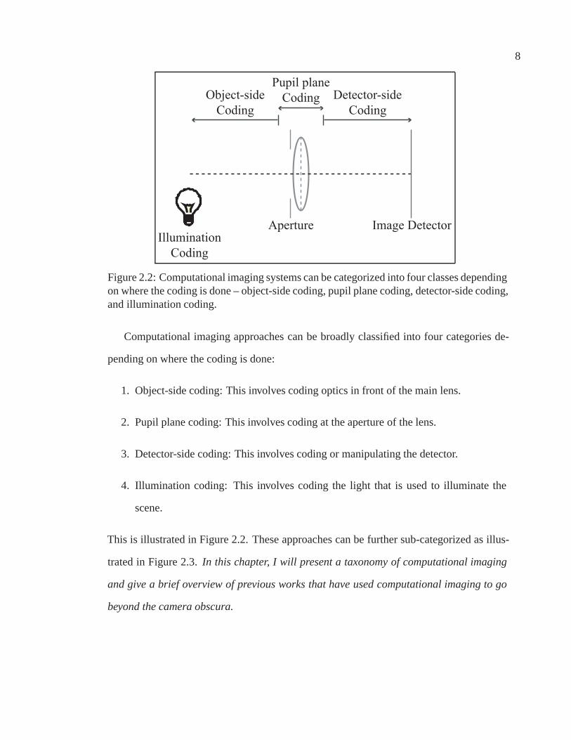
Figure 2.2: Computational imaging systems can be categorized into four classes dependingon where the coding is done – object-side coding, pupil plane coding, detector-side coding,and illumination coding.

Computational imaging approaches can be broadly classified into four categories de-

pending on where the coding is done:

1. Object-side coding: This involves coding optics in front of the main lens.

2. Pupil plane coding: This involves coding at the aperture of the lens.

3. Detector-side coding: This involves coding or manipulating the detector.

4. Illumination coding: This involves coding the light that is used to illuminate the

scene.

This is illustrated in Figure 2.2. These approaches can be further sub-categorized as illus-

trated in Figure 2.3. In this chapter, I will present a taxonomy of computational imaging

and give a brief overview of previous works that have used computational imaging to go

beyond the camera obscura.

9

Object-sideCoding

ReflectiveOptics

RefractiveOptics

TransmissiveOptics

Pupil PlaneCoding

ReflectiveOptics

RefractiveOptics

TransmissiveOptics

Detector-sideCoding

ReflectiveOptics

RefractiveOptics

TransmissiveOptics

Moving theDetector

NewDetectors

Figure 2.3: Object-side coding, pupil plane coding, and detector-side coding can be furtherclassified based on the coding strategy used.

2.2 Object Side Coding

This approach to computational imaging involves coding optics in front of the main lens

of the imaging system. Previous works can be divided into one of the following coding

strategies:

Reflective Optics

Mirrors have been used in conjunction with cameras for several applications in fields as

diverse as robotics, computer vision, computer graphics, and astronomy. Capturing large

fields of view has been a big motivation and spherical, hyperboloidal, ellipsoidal, conical,

and paraboloidal mirrors have been used for robot navigation, surveillance, teleconfer-

10

encing, etc. [81, 198, 199, 104, 131]. There has also been work on characterizing the

projections that are obtained on using various mirrors. On using curved mirrors, typically,

the captured images are multi-perspective with their effective viewpoints lying on what

are known as caustic surfaces [15, 183]. Baker and Nayar [9] derived that rotationally

symmetric conic reflectors – hyperboloids, ellipsoids, and paraboloids – placed at certain

locations with respect to the camera can yield usable wide angled imaging systems with

a single effective viewpoint. This single viewpoint constraint is desirable as it enables

computing pure-perspective images from the captured wide angle image. Rees [153] ap-

pears to have been the first to use a hyperboloidal mirror in conjunction with a perspective

camera to achieve a large field of view system with a single effective viewpoint. In or-

der to make the imaging systems compact, Nayar and Peri [129], use multiple mirrors.

However, the images captured by these single viewpoint systems have spatially varying

resolution. Recently, Nagahara et al. [119] have proposed a two mirror system with a

single viewpoint, but yet constant resolution. There have also been efforts to calibrate sin-

gle viewpoint systems such as the works of Geyer and Daniilidis [51, 50, 52]. They have

also derived the epipolar geometry that exists between multiple images captured by such

systems and estimate the motion between them [53, 54].

It should be noted that fish-eye lenses [116] can also be used to capture large fields

of view. However, since lenses have different refractive indices for different wavelengths

of light, the captured images usually have chromatic aberration effects. Also, lenses are

limited in being able to capture a maximum field of view of about 180. With curved

mirrors, much larger fields of view can be captured. However, using curved mirrors has

the disadvantage that the reflection of the camera also appears in the image and so that part

of the image is not usable.

Some works have designed mirror shapes in order to achieve certain desired charac-

teristics of the captured image. For instance, Hicks and Bajcsy have designed mirrors to

get a wide field of view as well as near-perspective projection for a given plane in the

11

scene [75]. Chahl and Srinivasan, Conroy and Moore, Gaspar et al., Hicks and Perline,

and others have designed mirror shapes to achieve wide field of view images with constant

resolution characteristics [21, 23, 46, 78]. These approaches to design mirror shapes were

generalized by Swaminathan et al. [182] who proposed a technique to find a mirror shape

that (approximately) realizes a given scene-to-image mapping. Recently, Hicks et al. [76]

have shown that for any rotationally symmetric projection with a single virtual viewpoint,

a two-mirror rotationally symmetric system can be designed that realizes that projection

exactly.

Conventional cameras have a single viewpoint. However, for many applications, like

stereo, it is desirable to capture scenes from multiple viewpoints. Mirrors have been used

for capturing scenes from multiple viewpoints, instantly, within a single image. For recov-

ering the 3D structure of scenes using stereo, the simplest mirror-based systems consist of

one or more planar mirrors occupying a part or the entire field of view of the camera. Such

designs have been suggested by Goshtasby and Gruver [60], Inaba et al. [83], Mathieu

and Devernay [109], and Gluckman and Nayar [56] among others. The real viewpoint of

the camera is reflected in the planar mirror(s), yielding the virtual viewpoint(s). In these

systems, the field of view of the camera is divided among the multiple views and as a

result the field of view of each viewpoint is typically small. To make the field of view of

each viewpoint larger, Nene and Nayar [136] have proposed using two (or more) rotated

ellipsoidal or hyperboloidal mirrors placed such that one of the two foci of each mirror and

the real viewpoint of the camera are coincident. The effective viewpoints of this system

are the other foci of each mirror. Another design that yields multiple discrete viewpoints

is imaging two displaced paraboloids using an orthographic camera [136]. Some mirror-

based stereo systems have also been proposed that do not yield a discrete set of virtual

viewpoints. Examples include imaging the reflections of the scene in two spheres [130]

and the system of Southwell et al. [176] who use a rotationally symmetric mirror with two

lobes where each lobe corresponds to one set of virtual viewpoints.

12

Capturing the appearance of materials, involves imaging a sample from a large number

of viewing directions for each of a large number of illumination directions. Gonioreflec-

tometers are used to measure the Bidirectional Reflectance Distribution Function (BRDF)

of a material, and they typically consist of a single photometer that is moved in relation to

the sample surface, while the sample itself is moved with respect to the light source. This

is a very time-consuming process. Mirrors have been used to expedite this process. In par-

ticular a number of systems have used curved mirrors – hemi-spherical and ellipsoidal – to

capture a sample from a large number of viewing directions in a single image [192, 110].

In Mattison et al. [110], the sample is placed at one focus of the ellipsoid, while the cam-

era is placed at the other focus, so that all outgoing rays from the sample (within a certain

outgoing angle) after reflection in the mirror are captured by the camera. Ward [192] uses

a hemi-spherical mirror as an approximation to this imaging geometry.

Though, the systems of Ward and Mattison et al. could capture a large number of view-

ing directions in a single image, to capture the sample under different lighting directions,

a light source had to be physically moved over the sampling sphere of lighting directions.

This is usually cumbersome and time-consuming. Subsequent systems have tried to ad-

dress this by using a beam splitter to co-locate (or align) the camera and the light source.

For instance, in the BRDF measurement system of Dana [27], different illumination direc-

tions are obtained by translating an aperture in front of an aligned collimated light source.

In Mukaigawa et al. [118] and Ghosh et al. [55], a projector, co-located with the camera

was used as a light source. In Mukaigawa et al. [118] different illumination directions are

obtained by turning on different sets of pixels in the projector. Ghosh et al. [55] propose

to project basis illumination patterns and measure the BRDF directly in a basis represen-

tation, instead of measuring the BRDF and then computing a basis representation for it.

Consequently, their system allows for rapid BRDF measurement.

Mirrors have also been used to efficiently measure spatially varying BRDFs, also

known as Bidirectional Texture Functions (BTFs). Han and Perlin [67] construct a kalei-

13

doscope using planar mirrors and employ multiple reflections in them to image a texture

sample from several viewing directions (around 22) in a single image. In order to image

the texture under several illumination conditions, they use a beam-splitter to co-locate a

projector with the camera. By turning on appropriate pixels in the projector, they could

illuminate the texture sample from different illumination directions.

Curved mirrors have also been used for measuring properties of participating media.

For instance, Hawkins et al. [73] use a conical mirror in conjunction with a laser to mea-

sure the phase function.

Since curved mirrors enable the capture of large fields of view, they have also been

used to measure the illumination distribution in a scene for computer graphics applica-

tions. Miller and Hoffman [114], and Debevec [31] have used mirror spheres to construct

environment maps, while Unger el. [188] have used an array of mirror spheres to measure

the spatially varying illumination in a scene.

The above imaging systems yield fixed scene-to-image mappings; once the imaging

system has been built, it captures scenes in the same way. To realize some flexibility in

the mappings that are realized, some works have proposed using a planar array of planar

mirrors, like a Digital Micro-mirror Device (DMD), in front of the camera [77, 125]. By

setting different orientations of the mirrors, they propose to emulate different effective

mirror shapes. Unfortunately, current DMD technology does not provide the flexibility to

orient mirrors with arbitrary orientations. Moreover, if the mirrors are in arbitrary orienta-

tions, there would be small gaps between the mirrors which could give rise to diffraction

effects and affect image quality.

Refractive Optics

Refractive optical elements have also been used in conjunction with cameras to realize sys-

tems that capture images with multiple discrete viewpoints. Lee and Kweon [97] and Xiao

and Lim [196] use prisms to capture two to four views of the scene within a single image.

14

Gao and Ahuja [45] propose to place a tilted transparent plate in front of a conventional

camera and capture a sequence of images while the plate rotates. This produces a large

number of stereo pairs, which they use to compute a depth map of the scene. They also

use the captured images and the estimated depth map for super-resolution.

By capturing a scene from a large number of viewpoints, we can sample the light

field of the scene. With this objective, Georgiev et al. [48] have built a system of lenses

and prisms as an external attachment to a conventional camera that captures the scene

from a large number of viewpoints in a single image. Compared to traditional integral

photography approaches [105, 1, 137], their approach has lower sampling density in the

angular dimension of the light field, but they make up for it using view interpolation of

the measured light field. They demonstrate how their imaging system enables changing

the focus in post-processing, while producing images with higher spatial resolution than

conventional integral photography.

Transmissive Optics

Some works have used optical elements that modulate the light rays before they enter the

lens. Schechner and Nayar [163, 164, 165, 166] have explored rigidly attaching to the

camera different spatially varying filters, such as neutral density, spectral, and polarization

filters. They rotate the system and capture a sequence of images. Consequently, every

scene point is imaged multiple times, each time filtered differently. The information from

the multiple images is then combined to create high dynamic, multi-spectral, or polariza-

tion state wide field of view panoramas of the scene. The disadvantage here is that the

scene must remain constant while the imaging system rotates.

To capture high dynamic range images, Nayar and Branzoi [132] place in front of the

lens a spatial light modulator, like a liquid crystal, whose transmittance can be varied with

high resolution over space and time. By setting an appropriate transmittance function on

the modulator, their control algorithm, ensures that no pixel is saturated in the captured

15

image. Each captured image and its corresponding transmittance function are then used

to compute a high dynamic range image. A similar setup is used by Raskar et al. [150]

wherein they use an external liquid crystal modulator as a shutter. The shutter is turned

off and on using a pseudo-random binary sequence during the exposure time of a single

image. They show that when such an imaging system is used to capture images of moving

objects, the resulting motion blur kernels reduce the loss of high frequencies and so enable

simple and effective deconvolution given the size of the blur kernel specified by the user.

High frequency occlusion masks, like binary occluders, have also been placed between

the lens and the scene to estimate and eliminate veiling glare. Veiling glare is a global

illumination effect that arises due to multiple scattering within the lens and camera body.

Talvala et al. [184] translate the mask and capture a sequence of images from which

they compute the glare free estimate, similar to the technique of Nayar et al. [128] for

separating direct and indirect illumination of a scene.

Polarized filters have also been used to modulate the imaged illumination. Wolff and

Boult [194] and Nayar et al. [127] capture images of a scene with different orientations

of a polarizer. They show that from the captured images, for dielectrics, they can separate

the specular and diffuse components of the captured images by exploiting the fact that

for dielectrics the specular component is polarized while the diffuse component is not.

Schechner et al. [168] use two images captured with different polarization orientations to

separate the reflected and transmitted components that result from imaging a transparent

surface. By capturing two images outdoors with different polarization orientations and

taking into account the effects of atmospheric scattering Schechner et al. [162] showed

that they can remove haze from images.

16

2.3 Pupil Plane Coding

Pupil plane coding involves coding optics in the lens aperture of the imaging system. The

various approaches can be divided into the following coding strategies:

Reflective Optics

Mirrors have been used to split the aperture of the imaging system. Aggarwal and Ahuja

[5] use a pyramid shaped mirror behind the main lens to split the light emerging from the

aperture into pie shaped pieces. Each piece of the aperture is then imaged by a different

sensor with a different exposure setting. The multiple images, captured at the same time

instant, have different effective exposure times and can be fused together to yield a high

dynamic range image. Recently, Green et al. [62] have used mirrors to divide the aperture

of the lens into four annular regions. Relay optics are then used to direct the images cor-

responding to each aperture piece to a quadrant of the captured image. They demonstrate

using the four sub-images to compute scene structure and manipulate depth of field.

Refractive Optics

The principle of refraction has also been used to modify the light passing through the

aperture of the lens. A number of works have explored using phase masks in the lens

aperture, an approach called wavefront coding. Refraction through the phase mask causes

the captured image to be blurred. However, by using an appropriate phase mask, the blur

kernel can be made to be invariant to scene depth for a range of scene depths. Hence, the

captured image can be deconvolved with a single blur kernel to get a sharp, all in focus

image. Cathy and Dowski [34] were the pioneers of this approach and subsequently, there

have been several efforts in this direction [20, 149, 19]. The principle of wavefront coding

has been shown to be very versatile, with works showing how wavefront coding can be

used for recovering 3D scene structure and correcting chromatic aberrations [35, 191].

17

Transmissive Optics

Transmissive masks have also been used in the lens aperture to modulate the captured

light. Traditional cameras have circular apertures. For defocused scene points, circular

apertures severely attenuate a lot of frequencies. Hence, deconvolution is usually unable to

restore the captured images. As a result, in the field of optics, a number of unconventional

apertures were designed with the aim of capturing high frequencies with less attenuation.

Both, binary aperture patterns [193, 189] as well as continuous ones [142, 115] have been

proposed.

Busboom et al. [18] have proposed capturing multiple images with different binary

aperture patterns. The multiple images can then be combined to create images obtained

using a wide range of different aperture patterns. They show how such an approach can

be used to increase the signal-to-noise ratio of the reconstructed images. Subramanian et

al. [179] also capture multiple images with different binary patterns. They rotate an off-

centered aperture about the optical axis. As a result, points on the plane of focus remain

stationary, while points away from the plane of focus translate in the image – the motion

being a function of the distance from the plane of focus. Hence, they can use the captured

images to estimate scene structure.

Recently, Liang et al. [103] have proposed two prototypes with coded apertures to

capture the light field of a scene. One uses a moveable pattern scroll and the other a liquid

crystal array. One approach to capture a light field is to effectively slide a pinhole across

the lens aperture. However, this produces very dim and noisy images. So the authors

propose to use aperture patterns that multiplex many pinholes. The captured images are

then demultiplexed to get the light field, from which they compute scene structure and

then use that for synthetic refocusing.

Recently, Veeraraghavan et al. [190] and Levin et al. [100] have proposed using binary

aperture patterns in the lens aperture, with the aim of estimating scene structure from a

18

single image and then using that for computing all-focused as well as refocused images.

Veeraraghavan et al. propose using a broad-band aperture pattern that preserves high fre-

quencies and hence is well suited for computing an all-focused image. On the other hand,

Levin et al. propose using a pattern optimized for depth recovery – the depth dependent

blur kernels have a lot of zero crossings in their Fourier representations. However, as

shown by Dowski and Cathey [35], there is an inherent tradeoff between recovering scene

depth and computing an all-focused image using a coded aperture. Thus, the above two

works lie at the two extreme ends of this tradeoff, though it should be noted that depth

recovery for both the methods is not robust.

Depth from defocus applications can also benefit from using coding masks in the aper-

ture. Hiura et al. [79] proposed selecting the aperture pattern with the aim of controlling

the characteristics of the blur kernel. For instance, a pattern that acts as a high-pass or

band-pass filter could preserve useful information for depth measurement.

Lenses cannot be used to bend and focus high energy radiations like x-rays and gamma-

rays. So in astronomy to gather more light and reduce noise, masks such as the MURA

[61] have been used in apertures of lens-less telescopes. However, the coded aperture

approaches in astronomy are suitable only for point light sources and also do not work well

with lenses. In vision too, there has been work on lens-less imaging. Zomet and Nayar

[203] show that by using, as an aperture, a stack of attenuating layers whose transmittances

are controllable in space and time, we get an imaging system with a flexible field of view

– the field of view can be panned and tilted without any moving parts. Also, disjoint scene

regions can be captured without capturing scene regions in between.

2.4 Detector Side Coding

This approach to computational imaging involves adding new coding optics and/or devices

on the detector side of the imaging lens. Previous works that follow this principle can be

19

categorized into the following coding strategies.

Reflective Optics

Planar arrays of planar mirrors like a Digital Micro-mirror Device (DMD) have been used

between the lens and the image detector to modulate light. The mirrors of the DMD can

be set to be in one of two orientations. In one orientation, the mirror reflects light coming

through the lens aperture to the detector, while in the other mirror orientation no light is

reflected to the detector. The ability to control the orientation of the mirrors both spatially

and temporally has been exploited for high dynamic range imaging by Christensen et al.

[22], Nayar et al. [126], and Ri et al. [154], among others. By controlling the amount of

time that each mirror reflects light to the detector, we can ensure that no pixel in the cap-

tured image is saturated. We can use the known effective exposure time and the measured

intensity to then compute a high dynamic range image. Nayar et al. [126] also show how

a DMD enables optical processing, such as performing feature detection and appearance

matching in the optical domain itself.

Refractive Optics

A captured image is a 2D projection of the 4D light field entering the lens and incident on

the sensor – every pixel integrates over the 2D set of rays that arrive at it. However, for

measuring the light field we need to measure the amount of light traveling along each ray.

In order to undo the effect of the integration on the detector and capture each individual ray,

Lippmann [105] and Ives [84] proposed placing an array of micro-lenses at the detector.

This approach is known as integral photography. The captured image consists of an array

of micro-images, one for each micro-lens. The content of each micro-image varies slightly

depending on the position of the corresponding micro-lens in the lens array. Adelson

and Wang [1] and then Okano et al. [143] proposed using such an imaging system for

20

recovering scene structure. Recently, Ng et al. [137] have developed a compact system

and shown that by resorting the captured rays, we can manipulate the depth of field of

the imaging system. This technology is now being developed and commercialized by

RefocusImaging [82].

Transmissive Optics

A pixel only samples a particular part of the visual spectrum as determined by the color

filter placed on top of it2. Most conventional color cameras have a color filter array, like

the Bayer filter array, over the detector so that one of the primary colors – red, green, or

blue – is sampled at each pixel. To obtain the full color image, demosaicing algorithms

are used to interpolate the missing two-thirds of the data at each pixel [108, 64].

Filter arrays with filters having spatially varying transmittance values have also been

proposed. Nayar and Mitsunaga [133] use such a filter array so that adjacent pixels in

a captured image have different effective exposures. These measurements, from a single

image, are then combined to get a high dynamic range gray scale image at a small cost of

spatial resolution. This approach was later extended to high dynamic range color images

[134, 122].

With the aim of capturing high dynamic range wide field of view panoramas, Aggarwal

and Ahuja [4] have proposed placing a graded transparency mask in front of the detector.

Thus, every pixel has a different exposure level. If the camera is panned in order to capture

a wide field of view in multiple images, each scene point is captured under several different

exposures. Information from the multiple images can then be combined to get a high-

dynamic range panorama.

Recently, Veeraraghavan et al. [190] have proposed placing a mask with spatially vary-

ing transmittances between the lens and the detector to capture the 4D light field entering

2An exception are pixels on the Foveon X3 sensor [171] which simultaneously sample all three colorchannels – red, green and blue.

21

the camera. A high frequency sinusoidal mask creates spectral tiles of the light field in the

4D frequency domain. Taking the 2D Fourier transform of the sensed signal, re-assembling

the tiles into a 4D stack of planes and taking the inverse Fourier transform, gives the 4D

light field.

Moving the Detector

Some works have proposed moving the detector to code how the scene is captured. Ben-

Ezra et al. [11] propose moving the detector within the image plane instantaneously in

between successive video frames. The motion corresponds to moving the detector along a

square whose size is half of that of a pixel. Since the motion is in between frames motion

blur due to detector motion is avoided. They show that by applying super-resolution to

the captured video sequence in an adaptive manner that takes into account objects with

fast or complex motions, they can compute super-resolution video. Recently, Levin et

al. [99] have proposed moving the image detector perpendicular to the optical axis with

constant acceleration – first going fast in one direction, progressively slowing down until it

stops, and then picking up speed in the other direction – during the integration of a single

image. They show that this motion causes all scene points moving in a particular direction

to be blurred in the same way, irrespective of the actual velocities in the image. That is,

motion blur becomes invariant to the actual motion of a scene point in a particular direction.

Therefore, applying deconvolution with a single blur kernel gives a sharp, motion blur free

image.

New Detectors

To overcome limitations of conventional cameras several new detectors have been pro-

posed. Conventional detectors have limited dynamic range. To measure high dynamic

range, some works, like Handy [68] and Konishi et al. [90], have proposed CCD detectors

22

where each pixel has two sensing elements of different sizes and hence different sensi-

tivities. During image exposure, two measurements are made at every pixel which are

then combined to generate a high dynamic range measurement. However, this approach

reduces spatial resolution by at least a factor of two.

Another approach to create high-dynamic range sensors is to have a computational

unit associated with each pixel that measures the time it takes to attain full-well capacity

[16]. This time is inversely proportional to the image irradiance and can be used to make

the measurement. Serafini and Sodini [172] have proposed a CMOS detector where each

pixel’s exposure can be individually controlled. The exposure time of a pixel, set so that

it does not saturate, and the measured intensity can then be used to compute the high

dynamic range measurement.

Some works have proposed new layouts for pixels on the detector. Ben-Ezra et al.

[12] argue that an aperiodic tiling of the image plane is best for super-resolution. Finally,

Tumblin et al. [187] propose a novel way to capture a high dynamic range image. Instead

of measuring intensities directly, they propose to measure gradients of the log of the image

intensities and then use Poisson integration to compute the intensity values.

2.5 Illumination Coding

The works described above involve new optics or devices that modify a conventional cam-

era. Computational imaging also involves modifying the illumination in a scene, so that

coded illumination can enable capturing more/better scene information than a normal cam-

era. Since the illumination has to be controlled, these approaches can only be used in

restricted environments which enable one to control the lighting.

Some works have projected structured light patterns onto scenes which are then imaged

by conventional cameras. Analyzing the captured image with the knowledge of the pro-

jected pattern enables recovering scene structure [195, 135, 96, 157, 121, 89, 202, 117, 8].

23

Most cameras have an accompanying flash for illuminating dimly lit scenes. However, this

frequently changes the appearance of the scene. Using a pair of images – one taken with a

flash and one without – some works have shown how one can enhance the image captured

without a flash [38, 148]. Flash no-flash image pairs have also been used to extract mat-

tes of foreground objects [180]. Some works have proposed using multiple flash units on

cameras, for structure recovery [41], non-photorealistic rendering [151], and for reducing

specular reflections [42].

Cameras usually only capture three portions of the spectrum of a scene – red, green,

and blue. With the aim of capturing a hyperspectral image, Park et al. [146] have proposed

illuminating the scene with a cluster of light sources with different spectra, that are mul-

tiplexed to reduce the capture time when using a conventional RGB camera. Multiplexed

illumination has also been used for reducing noise when capturing scenes under multiple

light sources [167].

The light reflected from a scene consists of two components – direct and global. The

direct component consists of light rays that start from the light source, reflect off a scene

point once and are then captured by the camera. The global component consists of all other

light rays, that could have undergone interreflections, subsurface scattering, volumetric

scattering, etc. Though the light captured by a camera almost always has both direct and

global components, many applications in vision assume that the captured light has only

the direct component. Recently, coded illumination techniques have been used to separate

reflection components. Nayar et al. [128] have shown that by capturing a sequence of

images while illuminating a scene using high frequency binary illumination patterns, one

can separate the direct and global components of the scene. Lamond et al. [95] have used

similar ideas to separate specular and diffuse reflection components.

In this thesis we propose three new computational imaging systems. Two of them –

Radial imaging systems and Flexible Field of View imaging systems (described in Chapters

3 and 4, respectively) – fall in the category of reflective object side coding. The third –

24

Flexible Depth of Field imaging system – is an example of detector side coding by moving

the detector. It is described in Chapter 6.

Chapter 3

Radial Imaging Systems

Many applications in computer graphics and computer vision require the same scene to

be imaged from multiple viewpoints1. The traditional approach is to either move a single

camera with respect to the scene and sequentially capture multiple images [102, 59, 147,

174, 170], or to simultaneously capture the same images using multiple cameras located at

different viewpoints [87, 86]. Using a single camera has the advantage that the radiomet-

ric properties are the same across all the captured images. However, this approach is only

applicable to static scenes and requires precise estimation of the camera’s motion. Using

multiple cameras alleviates these problems, but requires the cameras to be synchronized.

More importantly, the cameras must be radiometrically and geometrically calibrated with

respect to each other. Furthermore, to achieve a dense sampling of viewpoints such sys-

tems need a large number of cameras – an expensive proposition.

In this chapter, we develop a class of imaging systems called radial imaging systems

that capture the scene from multiple viewpoints instantly within a single image2. As only

one camera is used, all projections of each scene point are subjected to the same radio-

metric camera response. Moreover, since only a single image is captured, there are no

1The work presented in this chapter appeared in the ACM Transactions on Graphics (also SIGGRAPH),2006. This is joint work with Shree K. Nayar.

2Although an image captured by a radial imaging system includes multiple viewpoints, each viewpointdoes not capture a ‘complete’ image of the scene, unlike the imaging systems proposed in [188, 101].

25

26

synchronization requirements. Radial imaging systems consist of a conventional camera

looking through a hollow rotationally symmetric mirror (e.g., a truncated cone) polished

on the inside. The field of view of the camera is folded inwards and consequently the

scene is captured from multiple viewpoints within a single image. As we will show, this

simple principle enables radial imaging systems to have the flexibility to solve a variety of

problems in computer vision and computer graphics. Specifically, we demonstrate the use

of radial imaging systems for the following applications:

Reconstructing Scenes with Fewer Ambiguities: One type of radial imaging system

captures scene points multiple times within an image. Thus, it enables recovery of scene

geometry from a single image. We show that the epipolar lines for such a system are

radial. Hence, unlike traditional stereo systems, ambiguities occur in stereo matching only

for edges oriented along radial lines in the image – an uncommon scenario. This inherent

property enables the system to produce high quality geometric models of both fine 3D

textures and macroscopic objects.

Sampling and Estimating BRDFs: Another type of radial imaging system captures

a sample point from a large number of viewpoints in a single image. These measurements

can be used to fit an analytical Bidirectional Reflectance Distribution Function (BRDF)

that represents the material properties of an isotropic sample point.

Capturing Complete Objects: A radial imaging system can be configured to look all

around a convex object and capture its complete texture map (except possibly the bottom

surface) in a single image. We show that by capturing two such images with parallax, by

moving the object or the system, we can recover the complete geometry of the object. To

our knowledge, this is the first system with such a capability.

In summary, radial imaging systems can recover useful geometric and radiometric

properties of scene objects by capturing one or at most two images, making them sim-

ple and effective devices for a variety of applications in graphics and vision. It must be

noted that these benefits come at the cost of spatial resolution – the multiple views are pro-

27

jected onto a single image detector. Fortunately, with the ever increasing spatial resolution

of today’s cameras, this shortcoming becomes less significant. In our systems we have

used 6 and 8 megapixel cameras and have found that the computed results have adequate

resolution for our applications.

3.1 Related Work

Several mirror-based imaging systems have been developed that capture a scene from mul-

tiple viewpoints within a single image [177, 136, 58, 57, 67]. These are specialized sys-

tems designed to acquire a specific characteristic of the scene; either geometry or appear-

ance. In this chapter, we present a complete family of radial imaging systems. Specific

members of this family have different characteristics and hence are suited to recover dif-

ferent properties of a scene, including, geometry, reflectance, and texture.

One application of multiview imaging is to recover scene geometry. Mirror-based,

single-camera stereo systems [136, 57] instantly capture the scene from multiple view-

points within an image. Similar to conventional stereo systems, they measure disparities

along a single direction, for example along image scan-lines. As a result, ambiguities arise

for scene features that project as edges parallel to this direction. The panoramic stereo

systems in [177, 58, 104] have radial epipolar geometry for two outward looking views;

i.e., they measure disparities along radial lines in the image. However, they suffer from

ambiguities when reconstructing vertical scene edges as these features are mapped onto

radial image lines. In comparison, our systems do not have such large panoramic fields of

view. Their epipolar lines are radial but the only ambiguities that arise in matching and

reconstruction are for scene features that project as edges oriented along radial lines in the

image, a highly unusual occurrence3. Thus, radial imaging systems are able to compute

the structures of scenes with less ambiguity than previous methods.

3Compared to panoramic stereo systems, in our systems, ambiguities arise for vertical scene edges onlyif they project onto the vertical radial line in the image.

28

Sampling the appearance of a material requires a large number of images to be taken

under different viewing and lighting conditions. Mirrors have been used to expedite this

sampling process. For example, Ward [192], Dana [27], Ghosh et al. [55], and Mukaigawa

et al. [118] have used curved mirrors to capture in a single image multiple reflections of

a sample point that correspond to different viewing directions for a single lighting condi-

tion. We show that one of our radial imaging systems achieves the same goal. It should be

noted that a dense sampling of viewing directions is needed to characterize the appearance

of specular materials. Our system uses multiple reflections within the curved mirror to

obtain dense sampling along multiple closed curves in the 2D space of viewing directions.

Compared to [192, 27, 55, 118], this system captures fewer viewing directions. However,

the manner in which it samples the space of viewing directions is sufficient to fit analytic

BRDF models for a large variety of isotropic materials, as we will show. Han and Per-

lin [67] also use multiple reflections in a mirror to capture a number of discrete views

of a surface with the aim of estimating its Bidirectional Texture Function (BTF). Since

the sampling of viewing directions is coarse and discrete, the data from a single image is

insufficient to estimate the BRDFs of points or the continuous BTF of the surface. Con-

sequently, multiple images are taken under different lighting conditions to obtain a large

number of view-light pairs. In comparison, we restrict ourselves to estimating the parame-

ters of an analytic BRDF model for an isotropic sample point, but can achieve this goal by

capturing just a single image. Our system is similar in spirit to the conical mirror system

used by Hawkins et al. [73] to estimate the phase function of a participating medium. In

fact, the system of Hawkins et al. [73] is a specific instance of the class of imaging systems

we present.

Some applications require imaging all sides of an object. Peripheral photography [29]

does so in a single photograph by imaging a rotating object through a narrow slit placed in

front of a moving film. The captured images, called periphotographs or cyclographs [170],

provide an inward looking panoramic view of the object. We show how radial imaging

29

systems can capture the top view as well as the peripheral view of a convex object in

a single image, without using any moving parts. We also show how the complete 3D

structure of a convex object can be recovered by capturing two such images, by translating

the object or the imaging system in between the two images.

3.2 Principle of Radial Imaging Systems

To understand the basic principle underlying radial imaging systems, consider the example

configuration shown in Figure 3.1(a). It consists of a camera looking through a hollow

cone that is mirrored on the inside. The axis of the cone and the camera’s optical axis are

coincident. The camera images scene points both directly and after reflection by the mirror.

As a result, scene points are imaged from different viewpoints within a single image.

The imaging system in Figure 3.1(a) captures the scene from the real viewpoint of the

camera as well as a circular locus of virtual viewpoints produced by the mirror. To see

this consider a radial slice of the imaging system that passes through the optical axis of

the camera, as shown in Figure 3.1(b). The real viewpoint of the camera is located at O.

The mirrors m1 and m2 (that are straight lines in a radial slice) produce the two virtual

viewpoints V1 and V2, respectively, which are reflections of the real viewpoint O. There-

fore, each radial slice of the system has two virtual viewpoints that are symmetric with

respect to the optical axis. Since the complete imaging system includes a continuum of

radial slices, it has a circular locus of virtual viewpoints whose center lies on the camera’s

optical axis.

Figure 3.1(c) shows the structure of an image captured by a radial imaging system.

The three viewpoints O, V1, and V2 in a radial slice project the scene onto a radial line

in the image, which is the intersection of the image plane with that particular slice. This

radial image line has three segments – JK, KL, and LM, as shown in Figure 3.1(c). The

real viewpoint O of the camera projects the scene onto the central part KL of the radial

30

P

Optical Axis

Virtual

Viewpoint Locus

Camera

Mirror

P

Optical Axis

V1

V2

O

m2

m1

(a) (b)

pp2

p1J

M

K

L

(c)

P

Optical Axis

Virtual

Viewpoint Locus

Optical Axis

P

Virtual

Viewpoint Locus

(d) (e)

Figure 3.1: (a) Radial imaging system with a cone mirrored on the inside that images the

scene from a circular locus of virtual viewpoints in addition to the real viewpoint of the

camera. The axis of the cone and the camera’s optical axis are coincident. (b) A radial

slice of the system shown in (a). (c) Structure of the image captured by the system shown

in (a). The scene is directly imaged by the camera in the inner circle, while the annulus

corresponds to reflections of the scene in the mirror. (d) Radial imaging system with a

cylinder mirrored on the inside. (e) Radial imaging system with a cone mirrored on the

inside. In this case, the apex of the cone lies on the other side of the camera compared to

the system in (a).

31

line, while the virtual viewpoints V1 and V2 project the scene onto JK and LM, respectively.

The three viewpoints (real and virtual) capture only scene points that lie on that particular

radial slice. If P is such a scene point, it is imaged thrice (if visible to all three viewpoints)

along the corresponding radial image line at locations p, p1, and p2, as shown in Figure

3.1(c). Since this is true for every radial slice, the epipolar lines of such a system are

radial. Since all radial image lines have three segments (JK, KL, and LM) and the lengths

of these segments are independent of the chosen radial image line, the captured image has

the form of a donut. The camera’s real viewpoint captures the scene directly in the inner

circle, while the annulus corresponds to reflection of the scene – the scene as seen from

the circular locus of virtual viewpoints.

Varying the parameters of the conical mirror in Figure 3.1(a) and its distance from the

camera, we obtain a continuous family of radial imaging systems, two instances of which

are shown in Figures 3.1(d) and 3.1(e). The system in Figure 3.1(d) has a cylindrical mir-

ror. The system in Figure 3.1(e) has a conical mirror whose apex lies on the other side of

the camera compared to the one in Figure 3.1(a). These systems differ in the geometric

properties of their viewpoint loci and their fields of view, making them suitable for differ-

ent applications. However, the images that they all capture have the same structure as in

Figure 3.1(c).

Multiple circular loci of virtual viewpoints can be generated by choosing a mirror that

reflects light rays multiple times before being captured by the camera. For instance, two

circular loci of virtual viewpoints are obtained by allowing light rays from the scene to

reflect atmost twice before entering the camera. In this case, the captured image will have

an inner circle, where the scene is directly imaged by the camera’s viewpoint, surrounded

by two annuli, one for each circular locus of virtual viewpoints. Later we show how such

a system with multiple circular loci of virtual viewpoints can be used.

For the sake of simplicity, we restrict ourselves to radial imaging systems with conical

and cylindrical (which is just a special case) mirrors, which appear as lines in the radial

32

vd

vrV1

V2

Orθ

β

l

Optical Axis

dm

1

m2

V1

V2

O ψ

φ

φ

dt

db

φ

Trinocular SpaceStrictly Binocular Space

(a) (b)

V1

V2

O

φ

φ/2δ

0.2 0.3 0.4 0.5 0.6 0.7 0.8 0.9 1−4

−2

0

2

4

6

8

Radial Distance on the Image PlaneLog (

Tangential R

esolu

tion)

(c) (d)

Figure 3.2: Properties of a Radial Imaging System. (a) Radial slice of the imaging systemshown in Figure 3.1(a). (b) The fields of view of the real and virtual viewpoints in aradial slice. (c) The orientation of a virtual viewpoint in a radial slice. (d) The tangentialresolution of an image captured by an imaging system with β = 12, r = 3.5 cm, andθ = 45 for a scene plane parallel to the image plane located at a distance of 50 cm fromthe camera’s real viewpoint. The radial distance is measured on the image plane at unitdistance from the camera’s real viewpoint.

slices. It should be noted that in general the mirrors only have to be rotationally symmetric;

they can have more complex cross-sections.

3.3 Properties of a Radial Imaging System

We now analyze the properties of a radial imaging system. For simplicity, we restrict

ourselves to the case where light rays from the scene reflect at most once in the mirror

before being captured by the camera. In Section 3.4.3, we will analyze a system with

33

multiple reflections. For illustration, we will use Figure 3.2 which shows a radial slice

of the system shown in Figure 3.1(a). However, the expressions we derive hold for all

radial imaging systems including the ones shown in Figures 3.1(d) and 3.1(e). A cone can

be described using three parameters – the radius r of one end (in our case, the end near

the camera), its length l, and the half-angle β at its apex, as shown in Figure 3.2(a). The

complete imaging system can be described using one more parameter – the field of view

(fov) 2θ of the camera4. To differentiate between the configurations in Figures 3.1(a) and

3.1(e), we use the following convention: if the cone’s apex and the camera lie on the same

side of the cone, β ≥ 0; else β < 0. Therefore, for the systems shown in Figures 3.1(a),

(d), and (e), β > 0, β = 0, and β < 0, respectively.

The near end of the cone should be placed at a distance d = rcot(θ) from the camera’s

real viewpoint so that the extreme rays of the camera’s fov graze the near end, as shown in

Figure 3.2(a). Such a d would ensure that the entire fov of the camera is utilized.

3.3.1 Viewpoint Locus

In Section 3.2 we saw that radial imaging systems have a circular locus of virtual view-

points. We now examine how the size and location of this circular locus varies with the

parameters of the system. Since the system is rotationally symmetric, we can do this anal-

ysis in 2D by determining the location of the virtual viewpoints in the radial slice shown

in Figure 3.2(a). The virtual viewpoints V1 and V2 in a radial slice are the reflections of the

camera’s real viewpoint O produced by the mirrors m1 and m2, respectively. The distance

of the virtual viewpoints from the optical axis gives the radius vr of the circular locus of

virtual viewpoints, which can be shown to be

vr = 2rcos(β )sin(θ −β )csc(θ). (3.1)

4The field of view of a camera in a radial imaging system is the minimum of the camera’s horizontal andvertical fields of view.

34

The distance (along the optical axis) of the virtual viewpoints from the real viewpoint

of the camera is the distance vd between the circular locus of virtual viewpoints and the

camera’s real viewpoint:

vd = −2r sin(β )sin(θ −β )csc(θ). (3.2)

It is interesting to note that when β > 0, as in the system shown in Figure 3.1(a), vd < 0,

implying that the virtual viewpoint locus is located behind the real viewpoint of the camera.

In configurations with β = 0, as in Figure 3.1(d), the center of the circular virtual viewpoint

locus is at the real viewpoint of the camera. Finally, the circular locus moves in front of

the camera’s real viewpoint for configurations with β < 0, as in the one shown in Figure

3.1(e).

The length of the cone determines how many times light rays from the scene reflect in

the mirror before being captured by the camera. Since in this section we consider systems

that allow light rays from the scene to be reflected at most once, from Figure 3.2(a) it can

be shown that the length l of the cone should be less than l ′, where

l′ = 2rcos(β )cos(θ −2β )csc(θ −3β ). (3.3)

For ease of analysis, from this point onwards we assume that l = l ′.

3.3.2 Field of View

We now analyze how the fov of the viewpoints in a radial slice depend on the parameters

of the imaging system. Consider the radial slice shown in Figure 3.2(b). As we can see,

the fov φ of a virtual viewpoint is the portion of the fov of the camera that is incident on

35

the corresponding mirror and is given by

φ = arctan(2cos(θ −2β )sin(θ)sin(θ −β )

sin(θ −3β )+2sin(θ)cos(θ −2β )cos(θ −β )). (3.4)

Therefore, the effective fov ψ of the real viewpoint of the camera is the remaining portion

of the camera’s fov, which is

ψ = 2(θ −φ). (3.5)

The number of image projections of any given scene point equals the number of viewpoints

in the corresponding radial slice that can ‘see’ it. This in turn depends on where the scene

point lies. If a scene point lies in the trinocular space – area common to the fovs of all

viewpoints in a radial slice – it is imaged thrice. On the other hand, if a point lies in the

binocular space – area common to the fovs of at least two viewpoints – it is imaged at least

twice. Figure 3.2(b) shows the trinocular and binocular spaces. The scene point in the

trinocular space closest to O is obtained by intersecting the fovs of the virtual viewpoints.

This point lies at a distance

dt = r sin(2θ −2β )csc(θ)csc(θ −2β ) (3.6)

from O. Similarly, by intersecting the effective fov of the camera’s real viewpoint and the

fov of a virtual viewpoint, we obtain the distance of the two scene points in the binocular

space closest to O as

db = r sin(2θ −2β )cos(θ −φ)csc(θ)csc(2θ −2β −φ). (3.7)

Examining the expression for dt tells us that for systems with β > 0 (Figure 3.1(a)), the

trinocular space exists only if θ > 2β . On the other hand, in configurations with β ≤ 0

(Figures 3.1(d) and 3.1(e)), the fovs of all viewpoints in a radial slice always overlap. Note

36

that the binocular space exists in all cases.

We define the orientation of a virtual viewpoint as the angle δ made by the central ray

in its fov with the optical axis, as shown in Figure 3.2(c). It can be shown, using simple

geometry, that δ is given by

δ = (θ − φ2−2β )t. (3.8)

Here, t = 1, if the central rays of the virtual viewpoint fovs meet in front of the camera’s

real viewpoint, i.e., the fovs converge, and t = −1 otherwise. It can be shown that when

β ≤ 0, the virtual viewpoint fovs always converge. When β > 0, the fovs converge only if

θ > 3β .

3.3.3 Resolution

We now examine the resolution characteristics of radial imaging systems. For simplicity,

we analyze resolutions along the radial and tangential directions of a captured image sep-

arately. As described in Section 3.2, a radial line in the image has three segments – one

for each viewpoint in the corresponding radial slice. Therefore, in a radial line the spatial

resolution of the camera is split among the three viewpoints. Starting from Figure 3.2(b),

using simple geometry, we can determine the length of the radial image line intercepted

by the bounding rays of the effective fov of the camera’s real viewpoint. From this we can

show that the ratio of the lengths of the line segments on a radial image line belonging to

the camera’s real viewpoint and a virtual viewpoint is cos(θ )cos(θ−2β ) . Therefore, for systems

with β > 0, β = 0, β < 0 (Figures 3.1(a), 3.1(d), 3.1(e)), in a radial image line, a virtual

view has respectively fewer, same, or more pixels than the effective fov of the camera’s

real viewpoint.

We now study resolution in the tangential direction. Consider a scene plane Πs parallel

to the image plane located at a distance w from the camera’s real viewpoint. Let a circle

of pixels of radius ρi on the image plane image a circle of radius ρs on the scene plane Πs;

37

the centers of both circles lie on the optical axis of the camera. We then define tangential

resolution, for the circle on the image plane, as the ratio of the perimeters of the two circles

= ρi/ρs. If a circle of pixels on the image plane does not see the mirror, its tangential

resolution is 1/w (assuming focal length is 1). To determine the tangential resolution for

a circle of pixels that sees the mirror, we need to compute the mapping between a pixel

on the image plane and the point it images on the scene plane. This can be derived using

the geometry shown in Figure 3.2(a). From this mapping we can determine the radius ρs

of the circle on the scene plane Πs that is imaged by a circle of pixels of radius ρi on the

image plane. Then, tangential resolution is given by

ρi/ρs =ρi sin(θ)(cos(2β )+ρi sin(2β ))

2r sin(θ −β )(cos(β )+ρi sin(β ))−wsin(θ)(ρi cos(2β )− sin(2β )). (3.9)

Note that tangential resolution is depth dependent – it depends on the distance w of the

scene plane Πs. For a given w, there exists a circle of radius ρi on the image plane, which

makes the denominator of the above expression zero. Consequently, that circle on the

image plane has infinite tangential resolution5, as it is imaging a single scene point – the

scene point on Πs that lies on the optical axis. This property can be seen in all the images

captured by radial imaging systems. In Section 3.4.3 we exploit this property to estimate

the BRDF of a material using a single image. The tangential resolution for a particular

radial imaging system with parameters: β = 12, r = 3.5 cm, θ = 45 and a scene plane at

a distance w = 50 cm is shown in Figure 3.2(d). For ease of visualization the tangential

resolution values are plotted on a logarithmic scale.

We have built several radial imaging systems which we describe next. The mirrors

in these systems were custom-made by Quintesco, Inc. The camera and the mirror were

aligned manually by checking that in a captured image the circles corresponding to the

two ends of the mirror are approximately concentric. In our experiments, we found that

5In practice, tangential resolution is always finite as it is limited by the resolution of the image detector.

38

very small errors in alignment did not affect our results in any significant way.

3.4 Cylindrical Mirror

We now present a radial imaging system that consists of a cylinder mirrored on the inside.

Such a system is shown in Figure 3.1(d). In this case, the half-angle β = 0.

3.4.1 Properties

Let us examine the properties of this specific imaging system. Putting β = 0 in Equations

3.1 and 3.2, we get vr = 2r and vd = 0. Therefore, the virtual viewpoints of the system

form a circle of radius 2r around the optical axis centered at the real viewpoint of the

camera. It can be shown from Equations 3.4 and 3.5 that, in this system, the fov φ of the

virtual viewpoints is always smaller than the effective fov ψ of the real viewpoint of the

camera. Another interesting characteristic of the system is that the fovs of its viewpoints

always converge. As a result, it is useful for recovering properties of small nearby objects.

Specifically, we use the system to reconstruct 3D textures and estimate the BRDFs of

materials.

3.4.2 3D Texture Reconstruction and Synthesis

A radial imaging system can be used to recover, from a single image, the depth of scene

points that lie in its binocular or trinocular space, as these points are imaged from multi-

ple viewpoints. We use a radial imaging system with a cylindrical mirror to recover the

geometry of 3D texture samples. Figure 3.3(a) shows the prototype we built. The camera

captures 3032×2008 pixel images. The radial image lies within a 1791×1791 pixel square

in the captured image. In this configuration, the fovs of the three viewpoints in a radial

slice intercept line segments of equal length i.e., 597 pixels on the corresponding radial

39

Camera Mirror Object Camera Mirror Sample

(a) (b)

Figure 3.3: Two radial imaging systems that use a cylindrical mirror of radius 3.5 cm andlength 16.89 cm. (a) System used for reconstructing 3D textures that has a Kodak DCS760camera with a Sigma 20mm lens. (b) System used to estimate the BRDF of a sample pointthat has a Canon 20D camera with a Sigma 8mm Fish-eye lens.

image line. An image of a slice of bread captured by this system is shown in Figure 3.4(a).

Observe that the structure of this image is identical to that shown in Figure 3.1(c).

Let us now see how we can recover the structure of the scene from a single image. To

determine the depth of a particular scene point, its projections in the image, i.e., corre-

sponding points, have to be identified via stereo matching. As the epipolar lines are radial,

the search for corresponding points needs to be restricted to a radial line in the image.

However, most stereo matching techniques reported in literature deal with image pairs

with horizontal epipolar lines [161]. Therefore, it would be desirable to convert the infor-

mation captured in the image into a form where the epipolar lines are horizontal. Recall

that a radial line in the image has three parts – JK, KL, and LM, one for each viewpoint

in the corresponding radial slice (See Figure 3.1(c)). We create a new image called the

central view image by stacking the KL parts of successive radial lines. This view image

corresponds to the central viewpoint in the radial slices. We create similar view images for

the virtual viewpoints in the radial slices – the left view image by stacking the LM parts of

successive radial lines and the right view image by stacking the JK parts. To account for

the reflection of the scene by the mirror the contents of each JK and LM lines are flipped.

Figures 3.4(b,c,d) shows the three 597× 900 view images constructed from the captured

40

image shown in Figure 3.4(a). Observe that the epipolar lines are now horizontal. Thus,

traditional stereo matching algorithms can now be directly applied.

For our 3D reconstruction results, we used a window-based method for stereo match-

ing with normalized cross-correlation as the similarity metric [161]. The central view

image (Figure 3.4(c)) was the reference with which we matched the left and right view

images (Figures 3.4(b) and 3.4(d)). The left and right view images look blurry in regions

that correspond to the peripheral areas of the captured image, due to optical aberrations

introduced by the curvature of the mirror. To compensate for this, we took an image of a

planar scene with a large number of dots. We then computed the blur kernels for different

columns in the central view image that transform the ‘dot’ features to the corresponding

features in the left and right view images. The central view image was blurred with these

blur kernels prior to matching. This transformation, though an approximation, makes the

images similar thereby making the matching process more robust. Once correspondences

are obtained, the depths of scene points can be computed. Shaded and reconstructed views

of the 3D texture of the bread sample – a disk of diameter 390 pixels – are shown in Figures

3.4(e) and (f).

To determine the accuracy of the reconstructions obtained, we imaged an object of

known geometry – the inside of a section of a hollow cylinder of radius 3.739 cm. The

captured image is shown in Figure 3.5(a), in which the curvature of the object is along the

vertical direction. We reconstructed 145 points along the vertical radial image line and fit

a circle to them, shown in Figure 3.5(b). The radius of the best-fit circle is 3.557 cm and

the RMS error of the fit is 0.263 mm, indicating very good reconstruction accuracy.

We would like to point out that we have used a simple stereo matching algorithm. A

large number of sophisticated stereo matching algorithms have been proposed [145] and

one would expect to get better results on using them on the images captured by our system.

However, it should be noted that the view images computed from our captured images

differ from traditional stereo images. In traditional stereo images, each image has a single

41

(a)

(b) (c) (d)

(e) (f)

Figure 3.4: (a) Image of a slice of bread captured by the system shown in Figure 3.3(a).(b, c, d) The left (b), central (c), and right (d) view images constructed from the capturedimage shown in (a). Note that the epipolar lines for these images are horizontal. (e, f)Shaded (e) and textured mapped (f) views of the reconstructed bread texture.

42

−2 −1 0 1 2 3

30

Y (in cm)

Z (

in c

m)

30.5

31

31.5

32

32.5

33

33.5

34 Best Fit CircleReconstructed Points

(a) (b)

Figure 3.5: Determining the reconstruction accuracy of the cylindrical mirror systemshown in Fig 3.3(a). (a) Captured image of the inside of a section of a hollow cylinder.(b) Some reconstructed points and the best fit circle corresponding to the vertical radialline in the image. (See text for details.)

viewpoint. On the other hand, in our view images, each row has a different viewpoint.

It would be interesting to evaluate how this small deviation affects stereo algorithms and

what modifications, if any, are needed.

Figures 3.6 (a, b, c) show another example of 3D texture reconstruction – of the bark

of a tree. Since we now have both the texture and the geometry, we can synthesize novel

3D texture samples. This part of our work is inspired by the tremendous success of 2D

texture synthesis methods [36, 37, 93] that, starting from an RGB texture patch, create

novel 2D texture patches. To create novel 3D texture samples, we extended the simple

image quilting algorithm of Efros and Freeman [37] to operate on texture patches that in

addition to having the three (RGB) color channels have another channel – the z value at

every pixel6.

6To incorporate the z channel, we made the following changes to [37]: (a) When computing the similarityof two regions, for the RGB intensity channels, we use Sum-of-Squared Differences (SSD), while for thez channel, the z values in each region are made zero-mean and then SSD is computed. The final error is alinear combination of intensity and z-channel errors. (b) To ensure that no depth discontinuities are createdwhen pasting a new block into the texture, we do the following. We compute the difference of the means ofthe z values in the overlapping regions of the texture and the new block. This difference is used to offset zvalues in the new block.

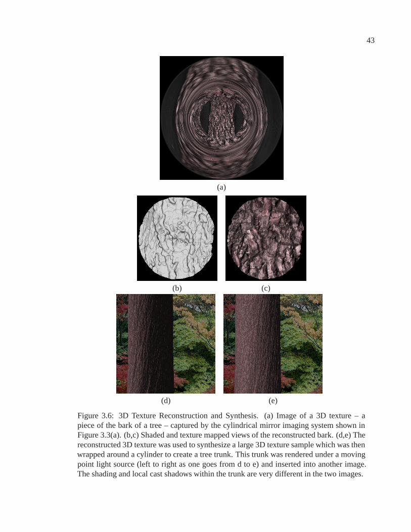
43

(a)

(b) (c)

(d) (e)

Figure 3.6: 3D Texture Reconstruction and Synthesis. (a) Image of a 3D texture – apiece of the bark of a tree – captured by the cylindrical mirror imaging system shown inFigure 3.3(a). (b,c) Shaded and texture mapped views of the reconstructed bark. (d,e) Thereconstructed 3D texture was used to synthesize a large 3D texture sample which was thenwrapped around a cylinder to create a tree trunk. This trunk was rendered under a movingpoint light source (left to right as one goes from d to e) and inserted into another image.The shading and local cast shadows within the trunk are very different in the two images.

44

The 3D texture shown in Figures 3.6(b, c) was quilted to obtain a large 3D texture

patch, which we then wrapped around a cylinder to create a tree trunk. This trunk was

then rendered under a moving point light source and inserted into an existing photograph

to create the images in Figures 3.6(d) and 3.6(e). The light source moves from left to right

as one goes from (d) to (e). Notice how the cast shadows within the bark of the tree differ

in the two images.

To recover the geometry of 3D textures Liu et al. [106] apply shape-from-shading

techniques to a number of images taken under different illumination conditions. These

images also come in handy at the time of texture synthesis as they can be used to impart

view dependent effects to the appearance of the new texture. In contrast, we capture both

the texture and the geometry of a 3D texture in a single image. However, since we have

only one image of the sample and do not know its material properties, we implicitly make

the assumption that the sample is Lambertian when we perform 3D texture synthesis.

3.4.3 BRDF Sampling and Estimation

We now show how a radial imaging system can be used to estimate the parameters of an

analytic BRDF model for an isotropic material. We make the observation that points on

the optical axis of a radial imaging system lie on all radial slices. Hence, if we place a

sample point on the optical axis of the system, it is imaged by all viewpoints. In fact, such

a point is imaged along a circle on the image plane – the tangential resolution for that

circle is infinite. We can get more viewpoints by letting light rays from the sample point

reflect in the mirror multiple times before being captured by the camera. As discussed

earlier, this would result in the sample point being imaged from several circular loci of

virtual viewpoints. It can be shown that the minimum length of the cylinder that is needed

for realizing n circular loci of virtual viewpoints is given by ln = 2(n−1)rcot(θ), n > 1.

The virtual viewpoints of this system form concentric circles of radii 2r, 4r, ··, 2nr.

Our prototype system, whose camera captures 3504×2336 pixel images, is shown in

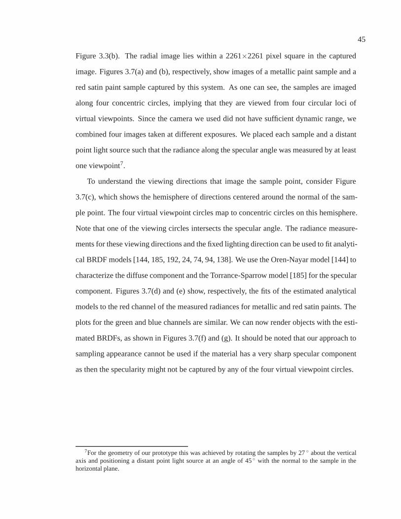
45

Figure 3.3(b). The radial image lies within a 2261×2261 pixel square in the captured

image. Figures 3.7(a) and (b), respectively, show images of a metallic paint sample and a

red satin paint sample captured by this system. As one can see, the samples are imaged

along four concentric circles, implying that they are viewed from four circular loci of

virtual viewpoints. Since the camera we used did not have sufficient dynamic range, we

combined four images taken at different exposures. We placed each sample and a distant

point light source such that the radiance along the specular angle was measured by at least

one viewpoint7.

To understand the viewing directions that image the sample point, consider Figure

3.7(c), which shows the hemisphere of directions centered around the normal of the sam-

ple point. The four virtual viewpoint circles map to concentric circles on this hemisphere.

Note that one of the viewing circles intersects the specular angle. The radiance measure-

ments for these viewing directions and the fixed lighting direction can be used to fit analyti-

cal BRDF models [144, 185, 192, 24, 74, 94, 138]. We use the Oren-Nayar model [144] to

characterize the diffuse component and the Torrance-Sparrow model [185] for the specular

component. Figures 3.7(d) and (e) show, respectively, the fits of the estimated analytical

models to the red channel of the measured radiances for metallic and red satin paints. The

plots for the green and blue channels are similar. We can now render objects with the esti-

mated BRDFs, as shown in Figures 3.7(f) and (g). It should be noted that our approach to

sampling appearance cannot be used if the material has a very sharp specular component

as then the specularity might not be captured by any of the four virtual viewpoint circles.

7For the geometry of our prototype this was achieved by rotating the samples by 27 about the verticalaxis and positioning a distant point light source at an angle of 45 with the normal to the sample in thehorizontal plane.

46

(a) (b)Normal Vector

Specular Reflection VectorLight Vector

Viewing Directions

−40 −20 0 20 40 60 800

50

100

150

200

250

Viewing Direction Elevation Angle (in degrees)

Inte

nsity

MeasuredPredicted by Model

Viewing Direction Elevation Angle (in degrees)−40 −20 0 20 40 60 800

50

100

150

200

250

Inte

nsity

MeasuredPredicted by Model

(c) (d) (e)

(f) (g)

Figure 3.7: BRDF Sampling and Estimation. (a) Image of a metallic paint sample cap-tured by the cylindrical mirror imaging system shown in Figure 3.3(b). (b) Image of a redsatin paint sample captured by the same cylindrical mirror imaging system. Observe thatthe samples are imaged along four concentric circles, corresponding to four circular lociof virtual viewpoints. (c) Plot showing the sample normal, light source direction, and theviewing directions for the captured images. (d, e) Plots comparing the measured radiancesin the red channel for different viewing directions, with those predicted by the fitted analyt-ical model for the (d) metallic paint and (e) red satin paint samples. (f,g) A model renderedwith the metallic and red satin paint BRDFs estimated from (a) and (b) respectively.

47

3.5 Conical Mirror

In this section, we present radial imaging systems with cones of different parameters. Hav-

ing unequal radii at the ends allows for greater flexibility in selecting the size and location

of the viewpoint locus and the fields of view.

3.5.1 Properties

As we discussed in Section 3.3, β is one of the parameters that defines a radial imaging

system. Let us consider separately the cases of β > 0 and β < 0. For systems with β > 0,

depending on the application’s needs, the virtual viewpoint locus can be varied to lie in

between the real viewpoint of the camera and vd =−r tan(θ/2). There is also flexibility in

terms of fields of view – the virtual viewpoint fovs can be lesser than, equal to, or greater

than the effective fov of the real viewpoint of the camera. Also, the viewpoint fovs may

converge or diverge. For systems with β < 0, the locus of virtual viewpoints can be varied

to lie in between the camera’s real viewpoint and vd = rcot(θ/2). Unlike configurations

with β > 0, in these systems the virtual viewpoint fovs are smaller than the effective fov

of the real viewpoint of the camera. Also, the viewpoint fovs always converge. Thus, such

systems are ideal for imaging nearby objects.

3.5.2 Reconstruction of 3D Objects

We now describe how to reconstruct 3D objects using a radial imaging system with β > 0

– like the one shown in Figure 3.1(a). Using a cylindrical mirror, as in the previous section,

causes the fovs of the viewpoints of the system to converge. Consequently, such a system

is suited for recovering the properties of small nearby objects. In order to realize a system

that can be used for larger and more distant objects, we would like the fovs of the virtual

viewpoints to ‘look straight’, i.e., we would like the central ray of each virtual viewpoint’s

fov to be parallel to the optical axis. This implies that δ – the angle made by the central ray

48

Camera Mirror Subject Camera MirrorObject

(a) (b)

Figure 3.8: Radial imaging systems comprised of a cone of length 12.7 cm and radii 3.4cm and 7.4 cm at the two ends. The half-angle at the apex of the cone is 17.48. Bothsystems use a Canon 20D camera. (a) System used for reconstructing objects such asfaces. A Sigma 8mm fish-eye lens was used in this system. (b) System used to capture thecomplete texture and geometry of a convex object. A Canon 18-55 mm lens was used inthis system.

in a virtual viewpoint’s fov with the optical axis – should be zero. Examining Equations

3.3 and 3.8 tells us that for this to be true the length of the cone has to be infinite – clearly

an impractical solution. Therefore, we pose the following problem: Given the fov of the

camera, the radius of the near end of the cone, and the ratio γ of the effective fovs of the

real and virtual viewpoints, determine the cone’s half-angle β at its apex and its length l.

A simple geometrical analysis yields the following solution:

β =θ(γ +1)2(γ +2)

, l =r sin(2θ/(γ +2))cos(β )

sin(θ)sin(θ(γ −1)/(2(γ +2))), γ > 1. (3.10)

The prototype we built based on the above solution is shown in Figure 3.8(a). The

radial image lies within a 2158×2158 pixel square of the 3504×2336 pixel captured image.

The effective fov of the camera’s real viewpoint intercepts 1078 pixels along a radial line

in the image. The fovs of the two virtual viewpoints intercept 540 pixels each. We have

used this system to compute the 3D structures of faces, a problem that has attracted much

interest in recent years. Commercial face scanning systems are now available, such as

those from Cyberware [25] and Eyetronics [39], which produce high quality face models.

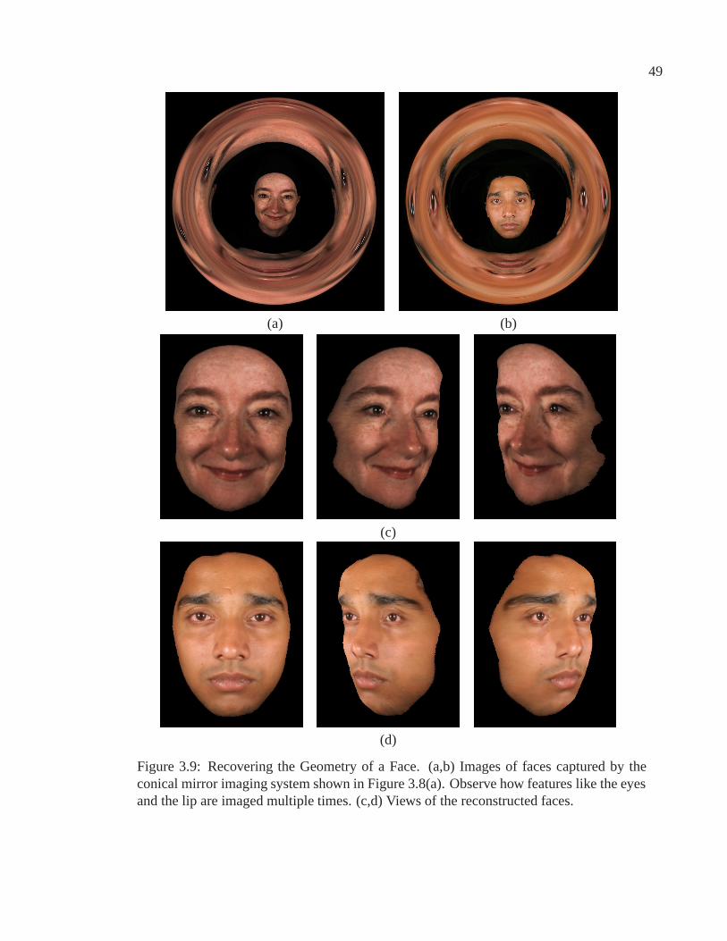
49

(a) (b)

(c)

(d)

Figure 3.9: Recovering the Geometry of a Face. (a,b) Images of faces captured by theconical mirror imaging system shown in Figure 3.8(a). Observe how features like the eyesand the lip are imaged multiple times. (c,d) Views of the reconstructed faces.

50

−6 −4 −2 0 2 4 6

36

38

40

42

44

46

Y (in cm)

Z (

in c

m)

Slice of the Reconstructed PlaneReconstructed Points

(a) (b)

Figure 3.10: Determining the reconstruction accuracy of the system shown in Figure 3.8(a).(a) Captured image of a plane. (b) Some reconstructed points and the slice of the best-fitplane corresponding to the vertical radial line in the image. (See text for details.)

However, these use sophisticated hardware and are expensive.

Figures 3.9(a) and (b) show two images captured by the conical mirror imaging system

in Figure 3.8(a). Since these images are identical in structure to those taken by the system

in Section 3.4.2, we can create the three view images, perform stereo matching and do

reconstruction as before. However, there is one small difference. In a radial slice, the

effective image line (analogous to the image plane) for a virtual viewpoint is the reflection

of the real image line. Since the mirrors are not orthogonal to the real image line in this

case, for any two viewpoints in a slice their effective image lines would not be parallel to

the line joining the two viewpoints. Therefore, before matching8two view images, they

must be rectified. For this, we project each row of the view images onto a line parallel to

the line joining the corresponding viewpoints.

Views of the 3D face models computed from the images in Figures 3.9(a) and (b) are

shown in Figures 3.9(c) and (d) respectively. To determine the accuracy of reconstructions

8Correspondence matches in specular regions (eyes and nose tip, identified manually) and texture-lessregions are discarded. The depth at such a pixel is obtained by interpolating the depths at neighboring pixelswith valid matches.

51

produced by this system, we imaged a plane placed 40 cm from the camera’s real viewpoint

and computed its geometry. The captured image is shown in Figure 3.10(a). The rms error

obtained by fitting a plane to the reconstructed points is 0.83 mm, indicating high accuracy.

Figure 3.10(b) shows the slice of the best-fit plane and some of the reconstructed points

corresponding to the vertical radial line in the captured image.

3.5.3 Capturing Complete Texture Maps of Convex Objects

We now show how a radial imaging system can be used to capture, in a single image, the

entire texture map of a convex object – its top and all sides (the bottom surface is not

always captured). To do so, the object must be imaged from a locus of viewpoints that

goes all around it. Therefore, the radius of the circular locus of virtual viewpoints should

be greater than the radius of the smallest cylinder that encloses the object; the cylinder’s

axis being coincident with the optical axis of the camera. Since radial imaging systems

with β < 0, like the one in Figure 3.1(e), have virtual viewpoint loci of larger radii, they

are best suited for this application. While the real viewpoint of the camera captures the top

view of the object, the circular locus of virtual viewpoints captures the side views. Thus,

the captured images have more information than the cyclographs presented in [170].

Figure 3.8(b) shows our prototype system. The radial image lies within a 2113×2113

pixel square of the 3504×2336 pixel captured image. In a radial slice, the effective fov of

the camera’s real viewpoint intercepts 675 pixels on the corresponding radial image line,

while the virtual viewpoints each intercept 719 pixels. Images of a conical and cylindrical

object captured by this system are shown in Figures 3.11(a) and (b) respectively. If we

know the geometries of these objects, we can use the captured images as texture maps, as

shown in the renderings in Figures 3.11(c) and (d), respectively.

The fields of view of the virtual viewpoints of the system slice through the object in

a radial fashion. Consequently, it is guaranteed to capture the complete texture maps of

convex objects. However, it also works for objects that are near convex, an example of

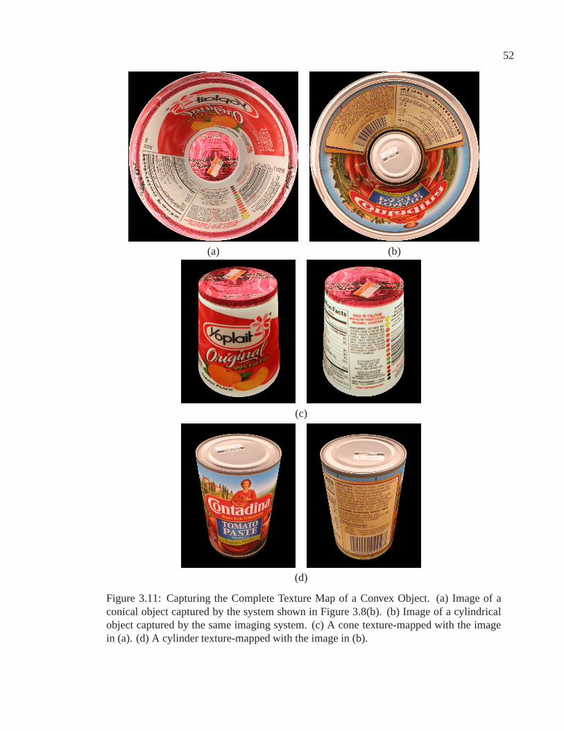
52

(a) (b)

(c)

(d)

Figure 3.11: Capturing the Complete Texture Map of a Convex Object. (a) Image of aconical object captured by the system shown in Figure 3.8(b). (b) Image of a cylindricalobject captured by the same imaging system. (c) A cone texture-mapped with the imagein (a). (d) A cylinder texture-mapped with the image in (b).

53

which we show in the next section.

3.5.4 Recovering Complete Object Geometry

We have shown above how the complete texture map of a convex object can be captured in

a single image using a radial imaging system with β < 0. If we take two such images, with

parallax, we can compute the complete 3D structure of the object. Figures 3.12(a) and (b)

show two images obtained by translating a toy head along the optical axis of the system

by 0.5 cm in between the two images9. Due to this motion of the object, the epipolar lines

for the two images are radial. In order to use conventional stereo matching algorithms, we

need to map radial lines to horizontal lines. Therefore, we transform the captured images

from Cartesian to polar coordinates – the radial coordinate maps to the horizontal axis.

As before, the two images are rectified. We then perform stereo matching on them and

compute the 3D structure of the object. Figure 3.12(c) shows some views of the recovered

complete geometry of the object shown in Figures 3.12(a) and (b). To our knowledge,

this is the first system capable of recovering the complete geometry of convex objects by

capturing just two images.

It should be noted that in this setup many scene features might project as radial edges

in a captured image, giving rise to ambiguities in matching. The ambiguity advantage

of having radial epipolar geometry (in Sections 3.4.2 and 3.5.2) is lost in this particular

configuration. Also, as in Section 3.5.3, this system is guaranteed to work for convex

objects. However, as the above example demonstrates, the system also works for objects

that are near convex.

9To move the object accurately, we placed it on a linear translation stage that was oriented to moveapproximately parallel to the camera’s optical axis.

54

(a) (b)

(c)

Figure 3.12: Recovering the Complete Geometry of a Convex Object. (a,b) Images of a toyhead captured by the imaging system shown in Figure 3.8(b). The toy head was translatedalong the optical axis between the capture of the two images. (c) Views of the recovered3D model of the toy head.

3.6 Discussion

In this chapter, we have introduced a family of imaging systems called radial imaging sys-

tems that capture a scene from the real viewpoint of the camera as well as one or more cir-

cular loci of virtual viewpoints, instantly, within a single image. We have derived analytic

expressions that describe the properties of a complete family of radial imaging systems.

We have demonstrated that this family has the flexibility that its different members can be

used to recover geometry, reflectance, and texture by capturing one or at most two images.

It should be noted that a number of systems have been developed in the past to capture

55

geometry and reflectance. In that light, our primary contribution is demonstrating the ex-

istence of this flexible family of imaging systems; the applications were used to show the

utility of this family.

Since our systems use curved mirrors, captured images are defocused due to mirror

curvature – especially at the boundaries of the images. To minimize these effects, we have

used large mirrors as well as small apertures. However, if the systems are to be made more

compact, we would have to account for this defocusing. One approach for tackling this

defocus problem is discussed in Chapter 5.

In this work, we have focused on the use of conical mirrors, which appear as lines in the

radial slices. In future work, we would like to explore the benefits of using more complex

mirror profiles. The virtual viewpoints of such imaging systems will not lie on circles

– they will lie on rotationally symmetric surfaces. However, they will enable capturing

scenes with desired non-uniform resolutions which might be useful for applications like

capturing texture maps. Another interesting direction is the use of multiple mirrors within

a system. We believe that the use of multiple mirrors would yield even greater flexibility in

terms of the imaging properties of the system, and at the same time enable us to optically

fold the system to make it more compact.

Chapter 4

Flexible Field of View

Traditional cameras have fields of view of fixed shapes – rectangular for perspective lenses

and circular for wide-angle lenses1. This severely restricts how scene elements can be

composed into an image. Therefore, an imaging system that provides control over the

shape and size of the field of view (FOV) would be desirable. Such an imaging system

would enable a photographer or an application to capture scenes in unconventional ways

– including only the scene elements of interest and excluding all other elements. In this

way, image pixels (a fixed resource) are devoted to capturing only what is desired. This is

particularly important in the case of video, where the number of pixels is always limited

by the fact that individual pixels must be large enough to collect sufficient photons within

a short integration time. Also, for dynamic scenes, this flexibility would enable one to

continuously vary the FOV as objects of interest move around. Such an ability is of value

in video monitoring applications.

In order to have control over the shape of the FOV, the camera must include some

form of flexible optics. In principle, it is possible to develop lenses with adjustable

shapes. While such elements have been proposed for finer optical adjustments such as

auto-focusing [158], they are hard to realize for our purpose of achieving a wide range of

1The work presented in this chapter appeared at the ICCV Omnivis Workshop, 2007. This is joint workwith Shree K. Nayar.

56

57

FOVs. We propose the use of a flexible mirror placed within the FOV of a perspective

camera. In its normal state the mirror is planar and hence the camera’s FOV remains un-

changed, except that it is rotated due to reflection by the mirror. By manually applying

forces to the boundary of the mirror, we can generate a wide and continuous range of

smoothly curved mirror shapes. Each shape results in a new FOV enabling us to capture

the scene in a new way.

Our system provides a convenient means to realize a wide range of scene-to-image

mappings. This is in contrast to traditional imaging systems that only provide a fixed or

limited set of fixed scene-to-image mappings. We believe that the flexibility to control this

mapping would open up a new creative dimension in photography and also be useful for

surveillance applications to react to changes in the scene.

Since we are capturing the reflections of the scene in a curved mirror, the captured

image looks distorted. In order to make the image usable we need to minimize these

distortions for which we have to know the 3D shape of the mirror when the image was

captured. Since the mirror shape can vary from one image to the next, it must be estimated

from the captured image itself. Towards this end, we have developed a simple calibration

method that estimates the 3D mirror shape from the 2D shape of its boundary, which is

visible in a captured image. Once we know the mirror shape, we can determine different

properties of the image, including its FOV and spatially varying resolution.

We have also developed an efficient algorithm that uses the estimated 3D mirror shape

to minimize distortions in the captured image; our algorithm maps the captured image to

an equi-resolution image – an image in which all pixels have the same field of view. To

do this, we do not need to know the geometry of the scene. Note that since our algorithm

digitally resamples a captured image, it does not improve on the captured image’s optical

resolution.

58

4.1 Related Work

A wide variety of catadioptric systems (imaging systems that use lenses and mirrors) have

been developed in fields as diverse as robotics, computer vision, computer graphics, and

astronomy. Wide-angle imaging is a popular application and some of these systems also

capture equi-resolution images [21, 23, 78]. However, in all these systems the mirror

shapes are fixed and hence their FOVs are not flexible. Recently, in [77, 126] it has been

suggested that a flexible mirror can be emulated using a planar array of planar mirrors,

where each planar mirror can be arbitrarily oriented. However, such a system is yet to

be implemented as there are no mirror arrays available that provide the required level

of control over mirror orientation. In astronomy, to remove the effects of atmospheric

turbulence, some telescopes use adaptive optics [156] in the form of membrane mirrors

that can change shape. Since such mirrors are used to adapt to phase changes in the

incoming radiation, their shapes vary over very small ranges and cannot be used to vary

FOV. Our system is similar in spirit to the flexible camera array of [139], in which many

cameras are mounted on a flexible sheet and the sheet is flexed to capture a scene using

an unconventional collective FOV. However, their objective is different. They combine

images from all their cameras to create a collage of the scene, while we map an image

captured by a single camera to a seamless undistorted composition of the scene.

Most techniques for calibrating catadioptric systems assume some knowledge of the

shape of the mirror [50, 88, 113]. Since the mirror shape can vary in our system, we can-

not make this assumption. In [159] the shape of a mirror is determined by analyzing how

it reflects a known calibration target, while in [63] a method is presented to calibrate a

generic imaging system by capturing a number of images of an active calibration target.

Since in our system the mirror can assume different shapes in different images, such ap-

proaches would mean repeating the complete calibration process for each image – a task

that is cumbersome for still images and impractical for videos with dynamic FOVs. To

59

45o

Camera

Flexible Mirror

22.5o

Figure 4.1: Prototype system that captures flexible FOVs.

address these issues, we present a method that determines the 3D shape of the mirror from

its 2D boundary in the captured image.

Since an image captured by our system is multi-perspective with varying resolution, it

has distortions. Recently, a framework was proposed to characterize such distortions [200].

One approach to minimize these distortions is to use user-specified scene priors [181]. To

handle arbitrarily complex and unknown scenes, we propose to minimize these distortions

by mapping a captured image to an equi-resolution image. This mapping problem may

also be formulated as an equi-areal projection of a sphere onto a plane [175]. However,

as we will show, for some imaging configurations this approach cannot be used due to

‘folding’ of the FOV. To address this problem, we have developed an alternative algorithm

to compute equi-resolution images.

4.2 Capturing Flexible Fields of View

The prototype system we built to capture flexible FOVs is shown in Figure 4.1. It com-

prises of a Panasonic PV-GS180 camcorder that captures the scene reflected in a flexible

planar mirror sheet. The camera captures 720×480 resolution video. The mirror sheet2 is

2Purchased on EBay for $20.

60

465×355 mm and made of acrylic. This sheet is mounted on another flexible plastic sheet

whose center is attached to the metallic frame. To deform the mirror, we simply apply

pressure on its edges or corners. As a guide, the user can look at the captured image which

is always visible in the camera’s LCD. We have used such a large mirror for two reasons.

First, optical aberrations due to the bending of the mirror decrease with mirror size and

hence are less noticeable in the captured image. Second, it is a convenient size for the user

to manually flex.

When we take a picture, the camera’s optical axis is usually parallel to the horizontal.

To mimic this, when the mirror is not deformed (it is planar), we would like the effective

viewpoint of our system to have a forward looking FOV. In our system, this is done by

elevating the camera’s optical axis by 45 and tilting the plane of the mirror by 22.5, as

shown in Figure 4.1. The horizontal FOV of the camera is 28.22 and the mirror is 60 cm

from the camera’s optical center.

As stated earlier, we estimate the 3D mirror shape from the shape of its boundary in

a captured image. To ensure that we can detect the mirror boundary robustly, we pasted

a trapezoidal border onto the mirror that is black with a thin white strip on the inside. A

trapezoidal border ensures that when the mirror is not deformed the reflective portion of

the mirror appears as a rectangle in a captured image.. This border can be seen in all the

captured images. The mirror boundary is automatically detected by searching from the

sides of the image inwards for a transition from black to gray. To represent the shape

of this boundary we choose 32 equidistant points on each ‘horizontal’ side and 24 on

each ‘vertical’ side. The coordinates of these 112 points are concatenated to form a 1D

descriptor, D , of the mirror boundary.

61

4.3 Determining Flexible Mirror Shape

To analyze a captured image, we need to know the shape of the mirror when the image

was taken. Here, we describe how the mirror shape can be estimated from its boundary in

a captured image.

4.3.1 Modeling Mirror Shape

The flexible mirror sheet can be deformed into various curved surfaces. These surfaces

are assumed to be smooth and we represent them using a tensor product spline similar to

how [66, 182] model a surface. Let M(u,v) be the 3D location of the point on the mirror

seen by image pixel (u,v), where (u,v) are normalized image coordinates. We represent

the z-coordinate Mz of this 3D point as

Mz(u,v) =Kf

∑i=1

Kg

∑j=1

ci j fi(u)g j(v). (4.1)

Here, fi and g j are 1D spline basis functions, ci j are the spline coefficients, and Kf and Kg

are the number of spline basis functions used along the u and v dimensions of the captured

image. The unknowns here are the spline coefficients ci j which would be different for

different deformations of the mirror. Once Mz(u,v) is known, the 3D mirror point is given

by M(u,v) = [u v 1]Mz(u,v). In our experiments, fi and g j are quadratic spline basis

functions and we use 6 such functions along each of the two spatial dimensions.

4.3.2 Off-line Calibration

It has been shown that for developable surfaces (like our planar flexible sheet) the 3D

boundary can be used to determine the 3D surface [32]. However, in our case, only the 2D

(image) shape of the boundary is known from the captured image and we need to deter-

mine the 3D mirror shape from it. More specifically, we need a mapping M between the

62

Mirror BoundaryProjected

Dot

Figure 4.2: One of the frames used for the off-line calibration of the 2D mirror boundaryto 3D mirror shape mapping. A thin white sheet was pasted on the mirror and a colorcoded dot pattern was projected on it using a projector. See text for details.

descriptor D of the mirror boundary (described in Section 4.2) and the spline coefficients

ci j in Equation 4.1 : ci j = M (D).

Since it is not clear that a closed-form solution to the mapping, M , can be found, we

precompute it as a look-up table using the following calibration procedure. We paste a thin

diffuse white sheet on the mirror surface and project a color-coded dot pattern on it using

a projector. The dots are color-coded and sparse so that we can easily establish correspon-

dences between the dots projected by the projector and the dots observed by the camera.

We then record videos of all mirror deformations that would be used to capture flexible

FOVs. We repeat each deformation a number of times. In all, we collected 30,753 frames,

one of which is shown in Figure 4.2. In each frame, we detect the mirror boundary and

compute its descriptor D . We also identify the projected dots (see Figure 4.2) and triangu-

late them with the projector to get 3D points on the deformed mirror. These reconstructed

points are then used to determine the spline coefficients ci j in Equation 4.1. The RMS

percentage errors for these fits were less than 0.05% per frame. The D and ci j for each

frame are used to construct the look-up table. Note that this is done off-line and only once.

After this, the thin diffuse white sheet is removed to reveal the reflective mirror surface.

63

Maximum values oferror measures

RMS Error 0.746%Median Error 0.417%

Max Error 2.763%

Table 4.1: Evaluation of our proposed technique to estimate the 3D shape of the mirrorfrom the 2D mirror boundary. We computed the RMS, maximum, and median percentageerrors in estimating the z coordinates of the mirror shape for each frame in our evaluationset. The maximum values of these over all frames in the evaluation set are shown here.

4.3.3 Estimating Mirror Shape for a Captured Image

For a captured image, the problem of finding the shape of the mirror is reduced to finding

the look-up table entry whose mirror boundary descriptor is closest (in L2) to that of the

given image. The corresponding spline coefficients are taken to determine the mirror shape.

Alternatively, one could find the k nearest entries in the table and interpolate among them.

In our experiments we picked the best matching entry and have found that it performs

well.

4.3.4 Evaluation

To validate our assumption that the boundary can be used to determine the mirror shape

we performed the following evaluation. We removed 1000 frames at random from the

calibration set to form a test set. We know the mirror shapes for these frames. Using

the look-up table we then ‘estimated’ the mirror shapes for these frames and compared

the z-coordinates of the actual and estimated shapes. The RMS percentage errors over

all frames was 0.0926%. We also computed the RMS, maximum, and median percentage

errors for each frame. The maximum values of these are shown in Table 4.1 and can be

seen to be small. This demonstrates that our assumption holds well for the smooth mirror

deformations we consider.

64

4.4 Properties of Captured Images

Once the mirror shape is known for a captured image, we can compute different properties

of the system that enable us to understand how the scene was mapped onto the image.

4.4.1 Viewpoint Locus

It has been shown that only rotationally symmetric conic mirrors placed at specific lo-

cations with respect to a perspective camera yield a single viewpoint [9]. Since in our

system the shape of the mirror is not necessarily a rotationally symmetric conic, it gen-

erally does not possess a single viewpoint, but rather a locus of viewpoints – a caustic

surface. Caustics of non-single viewpoint systems have been studied earlier [63] and we

employ the same approach to determine caustics for our systems3. Figure 4.3(a) shows an

image captured by our system where the mirror was flexed into a convex cylindrical shape

to increase the horizontal FOV. In Figure 4.3(b), the estimated mirror shape (gray surface)

and the corresponding caustic surface (blue surface) are shown.

4.4.2 Field of View

Since we know the shape of the mirror, for each pixel (x,y) in the image, we can trace back

the captured ray and determine its effective viewing direction Vx,y. This viewing direction

can be represented as a point on the surface of the unit sphere. In this way, we can map

each pixel of a captured image onto the unit sphere. We compute the FOV (effective solid

angle) imaged by a pixel (x,y) as the area of the spherical quadrilateral subtended on the

unit sphere by the viewing directions of pixels in a 2× 2 neighborhood whose top-left

3Once the mirror shape is known, we can determine the rays that are captured by the system, which wethen use to compute the caustic as in [63].

65

(a) Captured Image (b) Estimated Mirror Shapeand Caustic Surface

110o 145o 180o 215o 250o

80o

100o

120o

Azimuth

Ele

va

tion

110o 250o

80o

120o

θ

Φ

(c) Captured FOV (d) Resolution of Captured Image

Figure 4.3: (a) Image captured by our system where the mirror was flexed to increase thehorizontal FOV. (b) The gray surface represents the mirror shape estimated by our calibra-tion method, for the image in (a). The blue surface represents the resulting caustic. (c)FOV captured in the image in (a), shown using spherical panorama coordinates – θ (ele-vation angle) and φ (azimuth angle). (d) Resolution of the image in (a), where resolutionincreases from red to yellow.

pixel is (x,y). The FOV of a pixel can be easily shown to be

ωx,y =1

∑i=0

1

∑j=0

A(Vx+i,y+ j,Vx+1−i,y+ j,Vx+i,y+1− j), (4.2)

where, A(a,b,c) = −sin−1( (a×b)|(a×b)| .

(a×c)|(a×c)|). By adding the FOVs of all camera pixels that

see the mirror, we get the total FOV of the imaging system:

Ω =R−1

∑y=1

C−1

∑x=1

Px,yωx,y, (4.3)

66

where, the image is of size C×R and Px,y = 1, if pixel (x,y) sees the mirror and 0 otherwise.

Figure 4.3(c) shows the FOV captured in the image shown in Figure 4.3(a). The FOV is

shown using spherical panorama coordinates – θ (elevation angle) and φ (azimuth angle).

Additional examples can be seen in Figures 4.6(d), 4.8(d), 4.10(d), 4.11(d), and 4.12(d),

which show the FOVs captured in the images shown in Figures 4.6(b), 4.8(b), 4.10(b),

4.11(b) and 4.12(b), respectively. Note that though our camera has a horizontal FOV of

28.22 and a vertical FOV of 20.89, by using the flexible mirror, we are able to realize a

wide range of effective FOVs – the horizontal and vertical FOVs become as large as 120

and 40, respectively. The unconventional shapes of these FOVs enable us to compose

scenes in novel ways. Observe that in some cases the FOV even folds over (see Figures

4.11(d) and 4.12(d)).

4.4.3 Resolution

The resolution of a pixel in a captured image is defined [9] as ρ = Aω , where A is the area of

the pixel and ω is the solid angle of the scene imaged by that pixel (given by Equation 4.2).

Since all pixels occupy the same area on the image plane, the relative resolution of a pixel

is given by ρ = 1ω . Figure 4.3(d) shows the solid angle resolution map corresponding to the

captured image in Figure 4.3(a), where resolution increases from red to yellow. An image

captured by our system almost always has spatially varying resolution. The resolution

map allows us to visualize where the scene has been compressed or stretched in the image.

Additional examples can be seen in Figures 4.6(e) and 4.8(e) which show the solid angle

resolution maps of the captured images shown in Figures 4.6(b) and 4.8(b), respectively.

In addition to the solid angle resolution map, we can compute three additional resolu-

tion maps that represent (a) horizontal resolution, (b) vertical resolution, and (c) angular

resolution. To compute these quantities for a pixel (x,y), consider the spherical triangle

formed by the viewing directions of pixels (x,y), (x + 1,y), and (x,y + 1), i.e., by Vx,y,

Vx+1,y, and Vx,y+1, respectively. Horizontal resolution HRx,y is the length of the side of the

67

spherical triangle joining vertices Vx,y and Vx+1,y. Analogously, vertical resolution V Rx,y

is the length of the side joining Vx,y and Vx,y+1. Angular resolution ARx,y is the angle of

the spherical triangle at Vx,y. Together these three maps better capture how scene elements

are compressed or stretched in an image than does the solid angle resolution map alone.

We will use these maps to undistort the captured images. Note that given the horizontal,

vertical and angular resolution maps, we can directly compute the solid angle of a pixel

(x,y) as

ωx,y =1

∑i=0

2 tan−1(li sin(ARx+i,y+i)

1+ li cos(ARx+i,y+i)), (4.4)

where,

li = tan(HRx+i,y

2) tan(

V Rx,y+i

2). (4.5)

4.5 Undistorting Captured Images

We propose to minimize the distortions in a captured image, without having to know scene

geometry, by mapping a captured image to an equi-resolution image – an image where all

pixels correspond to equal solid angles.

4.5.1 Creating Equi-Resolution Images

One approach to create an equi-resolution image is to map all pixels in a captured image

onto the surface of a unit sphere (as discussed in Section 4.4.2) and then project the sphere

onto a plane using an equi-areal projection such as Mollweide, Hammer, etc. [175]. These

are 1-1 bijective mappings from a sphere onto a plane. However, this approach cannot

be used if the FOV folds over (see Figures 4.11(d) and 4.12(d)) i.e., if multiple points on

the image plane map to the same point on the sphere. In such cases, since the mapping

68

between the sphere and the captured image is not 1-1, a 1-1 mapping between the equi-

resolution image and the captured image does not exist.

Proposed Algorithm

We propose an alternative algorithm to compute equi-resolution images from captured im-

ages that can be used even if the FOV folds over. Our algorithm has four steps:

1. Compute the four resolution maps – solid angle resolution, horizontal resolution,

vertical resolution and angular resolution (Section 4.4.3).

2. Determine the smallest solid angle in the captured image from the solid angle res-

olution map and use that as the target solid angle – the solid angle that we want all pixels

in the equi-resolution image to have. This is denoted by t.

3. Stretch the captured image, denoted by IC, horizontally (retain pixel y-coordinates),

keeping the center column fixed, so that all pixels have the same horizontal resolution, de-

noted by a. The resulting image is denoted by IH .

4. Stretch IH vertically (retain pixel x-coordinates), keeping the center row fixed so

that the vertical resolution along the center column is a and the solid angle at all pixels is

t. The resulting equi-resolution image is denoted by IE .

We now explain steps 3 and 4 in greater detail. For step 3, the target horizontal resolu-

tion a has to be specified. A good estimate of a can be automatically computed from the

target solid angle t, as described in Appendix A. This is the approach we have used for all

examples in this chapter. Alternatively, the value of a can be specified by the user. Given a,

we linearly sample each row of IC starting from the center column and moving outwards,

such that the horizontal resolution at each pixel is a. For this, we use IC’s horizontal

69

Center Column

d0 d1 d2d-1d-2

e 0 e 1 e 2e -1e -2

HH

G

(a) (b)

Figure 4.4: Illustrations of steps 3 and 4 in the computation of equi-resolution images. Seetext for details.

resolution map. This process is illustrated in Figure 4.4(a). The grid represents the pixel

grid of IC, while the gray circles represent the sample points for the horizontally stretched

image IH . Since this image will be used as the input for the next step, we need its vertical

and angular resolution maps, which can be computed from IC’s resolution maps.

In step 4, we construct the equi-resolution image IE , row by row, starting from the

center. Consider the pixel grid of IH shown in Figure 4.4(b). The gray circles di represent

pixels on the center row of IH as well as IE , d0 being the center pixel. We construct the

row above the center row beginning with the sample e0 in the center column. Since a is

the vertical resolution along the center column of IE , the vertical resolution at e0 should

be a. Hence, we can use the vertical resolution map of IH to determine e0’s y-coordinate.

Also, the area of the spherical quadrilateral corresponding to e0, d0, d1, and e1 should be

t – the target solid angle. Given e0, the vertical resolution at e1 that would satisfy this is

given by

v1 = 2tan−1(sin( (t−m1)

2 )

sin((H −G)− (t−m1)2 ) tan(n1

2 )), (4.6)

where m1 is the area of the spherical triangle formed by e0,d0, and d1, H is the angular

resolution at d1, G is the spherical angle between the sides corresponding to e0d1 and d0d1

(see Figure 4.4(b)), and n1 is the arc length on the sphere corresponding to e0d1. The value

of v1 can be used to determine the y-coordinate of e1. Similarly, the location of e1 can be

used to determine the location of e2. The same technique can be applied to compute all eis.

70

Due to numerical issues, the ei sequence might not be smooth. To ensure smoothness, we

fit a cubic approximating spline to the ei values and obtain smoother estimates ei. These

smoothed eis form a row4 of IE . All other rows of IE can be constructed similarly.

As discussed in Section 4.4.2, in some configurations the FOV folds over (see Figures

4.11(d) and 4.12(d)). In such cases, the boundary of the fold (where the FOV starts fold-

ing over – a band 5-10 pixels wide) has very small solid angles – as much as 200 times

smaller than the solid angles at other points in the image. Consequently, these regions

project onto very small areas in the equi-resolution image, i.e., the image looks ‘pinched’

in these regions. Therefore, we consider such regions as anomalies and substitute the hor-

izontal, vertical and angular resolutions at such points by interpolating the resolutions at

neighboring points.

Evaluation

To evaluate the ability of our technique to minimize distortions we performed the follow-

ing simulation. We constructed a synthetic scene with a large number of black spheres

arranged on a tessellated sphere obtained by recursively subdividing an icosahedron. We

then rendered the scene as reflected in a convex cylindrical mirror and a concave cylindri-

cal mirror5. The rendered images are respectively shown in Figures 4.5(a,c) in which the

spheres are severely distorted and unevenly spaced. The solid angle resolution maps for

these images are shown in Figures 4.5(b,d). As one can see, the resolution varies over the

entire image. Figures 4.5(e,g) show the equi-resolution images computed from the ren-

dered images. Note that the spheres are almost circular and evenly spaced, demonstrating

that our mapping minimizes local distortions. Their corresponding solid angle resolution

maps are shown in Figures 4.5(f,h). The RMS percentage errors are 0.04% and 0.03%,

respectively.

4Note that to construct additional rows above this row, we need to determine the horizontal and angularresolution in IE at all ei. These can be computed from IH ’s resolution maps.

5The mirrors were rotated about the horizontal axis to mimic the configuration in our physical setup.

71

(a) (b) (c) (d)

(e) (f)

(g) (h)

(i) (j)

(k) (l)

Figure 4.5: (a,c) Renderings of a scene with black spheres reflected in (a) a convex cylin-drical mirror and (c) a concave cylindrical mirror. In both cases the curvature is alongthe horizontal. The spheres are arranged on a tessellated sphere obtained by recursivelysubdividing an icosahedron. (b,d) Solid angle resolution maps for the images in (a,c). (e,g)Equi-resolution images computed from (a,c). Note that the spheres are almost circular andevenly spaced, demonstrating that our mapping minimizes local distortions. (f,h) Solidangle resolution maps of the equi-resolution images in (e,g). (i,k) Rectangular imagescomputed from the equi-resolution images in (e,g). (j,l) Solid angle resolution maps of therectangular images in (i,k).

72

4.5.2 Creating Rectangular Images

Equi-resolution images do not have rectangular boundaries and look odd since we are

used to seeing rectangular images. We can correct this by applying an image warp to the

equi-resolution image that maps its boundary to the boundary of a rectangle. Since, we

are starting from an equi-resolution image, in most cases, this additional warping does not

introduce much distortion. To compute this warp, we need to establish correspondence

between the boundaries of the equi-resolution image and the output rectangular image.

This is done as follows. We discretize the ‘horizontal’ and ‘vertical’ sides of the boundary

of the equi-resolution image so that they have p and q equidistant points, respectively6.

The longer of the two horizontal sides and the two vertical sides determine the width and

height of the rectangular image, respectively. Like the boundary of the equi-resolution

image, the horizontal and vertical sides of the rectangle are also discretized to have p

and q equidistant points, respectively, thereby establishing correspondences between the

two boundaries. These correspondences are used to setup a thin-plate spline based image

warp [14, 98] that maps points (m,n) in the rectangular image to points (r,s) in the equi-

resolution image. This warp consists of two maps Fr : (m,n) → r and Fs : (m,n) → s,

both of which minimize the energy

∫ ∫σ[(

∂ 2F

∂ 2m)2 +2(

∂ 2F

∂m∂n)2 +(

∂ 2F

∂ 2n)2]dmdn, (4.7)

where σ is the domain of the rectangular image. Figures 4.5(i,k) show the rectangular im-

ages computed from the equi-resolution images in Figures 4.5(e,g). Their corresponding

solid angle resolution maps are shown in Figures 4.5(j,l). Note that the rectangular images

have almost uniform resolution and low distortion.

6In our experiments, we used p = 32 and q = 24.

73

(a) (b)

120O 240 O

110 O

80O

Φ

θ

(c) (d) (e)

Figure 4.6: (a) Image captured when the mirror is not flexed. (b) Image captured by flexingthe mirror to include all 7 people in the FOV. (c) Estimated mirror shape. (d) FOV capturedin (b). (e) Solid angle resolution map of the image in (b).

4.6 Examples

We now present a number of scene compositions captured by our flexible FOV imaging

system.

Birthday Snap: Often, when taking a picture of a group of people, like at a birthday , not

everyone fits in the picture – we need a larger horizontal FOV (see Figure 4.6(a)). The

image in Figure 4.6(a) was captured by our system when the mirror was not flexed. Figure

4.6(b) shows the picture captured by flexing the mirror’s two vertical edges and deforming

it into a convex cylindrical shape. All 7 people now fit in the FOV. The estimated mirror

shape and the resulting FOV are shown in Figures 4.6(c) and 4.6(d), respectively. Note that

the horizontal FOV (121.72) is much larger than the vertical FOV (20.25) – the effective

aspect ratio is very different from that of the image detector. Note that, in principle, one

74

(a)

(b)

(c) (d)

Figure 4.7: (a) Equi-resolution image computed from the captured image shown in 4.6(b).(b) Rectangular image computed from the image in (a). (c,d) Solid angle resolution mapsof the images in (a) and (b) respectively.

could have captured all the desired scene elements in an image using a wide-angle lens.

However, in that case, since the shape of the FOV is fixed, the camera would capture

scene elements that are not needed, i.e., image pixels would be ‘wasted’ on undesired

elements. In contrast, in our system, we can adjust the shape of the FOV, so that image

pixels are devoted to capturing only the scene regions of interest. The spatially varying

solid angle resolution of the image in Figure 4.6(b) is shown in Figure 4.6(e). The equi-

resolution image computed from the captured image in Figure 4.6(b) is shown in Figure

4.7(a) and its solid angle resolution map is shown in Figure 4.7(c). Figure 4.7(b) shows the

rectangular image computed from the image in Figure 4.7(a). Its resolution map is shown

in Figure 4.7(d). The image shown in 4.6(b) is a frame from a video sequence where the

75

(a) (b)

130o 220oΦ130o

90o

θ

(c) (d) (e)

Figure 4.8: (a) Image captured when the mirror is not flexed. (b) Image captured byflexing the mirror to include the butterfly (while excluding the scene region above it) andto include the person on the left. (c) Estimated shape of the mirror for the image in (b). (d)FOV captured in (b). (e) Solid angle resolution map of the image in (b).

FOV was changed over time. The video sequence as well as the computed undistorted

video sequences can be seen at [141].

Conversation: Figures 4.8(a) and (b) show two frames from a video sequence where the

FOV was changed over time as a conversation progressed. The frame in Figure 4.8(a) was

captured when the mirror was not flexed. For the frame in Figure 4.8(b) the mirror was

flexed to include the butterfly (while excluding undesirable scene elements above it) and

the left side of the mirror was flexed to include the person on the left. Figure 4.8(c) shows

the shape of the mirror estimated by our calibration method. The resulting FOV is shown

in Figure 4.8(d) and can be seen to have a rather complex shape. The spatially varying

solid angle resolution of the image in Figure 4.8(b) is shown in Figure 4.8(e). The equi-

resolution image computed from the captured image in Figure 4.8(b) is shown in Figure

76

(a)

(b)

(c) (d)

Figure 4.9: (a) Equi-resolution image computed from the captured image shown in 4.8(b).(b) Rectangular image computed from the image in (a). (c,d) Solid angle resolution mapsof the images in (a) and (b) respectively.

4.9(a) and its solid angle resolution map is shown in Figure 4.9(c). As one can see the

equi-resolution image has uniform resolution. Figure 4.9(b) shows the rectangular image

computed from the image in Figure 4.9(a). Its resolution map is shown in Figure 4.9(d).

These video sequences can be seen at [141].

Panning Up: Figure 4.10(a) shows an image captured by our system when the mirror was

not flexed. One can see only the feet of a person. Figure 4.10(b) shows the image captured

on flexing the top edge of the mirror to include the complete person. The estimated mirror

shape is shown in Figure 4.10(c), while Figure 4.10(d) shows the captured FOV. Note that

in this case, the vertical FOV is larger than the horizontal FOV. Figures 4.10(e) and 4.10(f)

show the computed equi-resolution image and rectangular image, respectively.

77

(a) (b)

150o 210oΦ100o

60o

θ

(c) (d)

(e) (f)

Figure 4.10: (a) Captured image when the mirror is not flexed. (b) Captured image whenthe mirror’s top edge is flexed. (c) Estimated mirror shape for the image in (b). (d) FOVcaptured in image in (b). (e) Equi-resolution image computed from the image in (b). (f)Rectangular image computed from the image in (e).

78

Street Monitoring: Figure 4.11(a) shows a street captured when the mirror is not flexed.

The ability to change the FOV enables our system to see the buildings on the sides of the

street and the sky (top edge flexed) in Figure 4.11(b) and the left side of the street (left edge

flexed) in Figure 4.12(b). Figures 4.11(c) and 4.12(c) show the corresponding estimated

mirror shapes. The captured FOVs are shown in Figures 4.11(d) and 4.12(d), respectively.

Figures 4.11(e) and 4.12(e) show the equi-resolution images computed from the images in

Figures 4.11(b) and 4.12(b), respectively. The undistorted rectangular images computed

from the equi-resolution images are shown in Figures 4.11(f) and 4.12(f), respectively.

These results demonstrate that the proposed imaging system enables us to compose

scenes in ways not possible before – to include only the scene elements of interest and

exclude all others. In this way image pixels are devoted only to the desired scene elements.

The use of a flexible mirror enables our system to realize a wide range of scene-to-image

mappings. This not only opens up a new creative dimension in photography, but can also

be useful for surveillance applications.

4.7 Discussion

Though the proposed approach enables us to compose scenes in novel ways, it has certain

limitations. Different fields of view are obtained by deforming the mirror to get various

curved surfaces. Focusing on the reflections of a scene in a curved mirror is known to be

difficult due to optical aberrations introduced by the curvature of the mirror. The entire

scene is usually not in focus. In our implementation, these effects are not noticeable as we

have used a large mirror – for any given shape, a larger mirror has lower local curvatures

and hence produces less blurring due to aberrations. However, if the system is to be made

compact (use a smaller mirror), or if a high resolution sensor is to be used, we would have

to account for this blurring. One approach for this, which is examined in more detail in

Chapter 5, is to use a post-processing step. If needed, we first perform a calibration to

79

(a) (b)

150o 210oΦ100o

60o

θ

Folding of the FOV

(c) (d)

(e) (f)

Figure 4.11: (a) Captured image when the mirror is not flexed. (b) Captured image whenthe mirror’s top edge is flexed. (c) Estimated mirror shape for the image in (b). (d) FOVcaptured in image in (b). (e) Equi-resolution image computed from the image in (b). (f)Rectangular image computed from the image in (e).

80

(a) (b)

Φ130o 190o105o

80 o

θFolding of the FOV

(c) (d)

(e)

(f)

Figure 4.12: (a) Captured image when the mirror is not flexed. (b) Captured image whenthe mirror was flexed to include the left side of the street. (c) Estimated mirror shapefor the image in (b). (d) FOV captured in the image in (b). (e) Equi-resolution imagecomputed from the image in (b). (f) Rectangular image computed from the image in (e).

81

estimate the optical properties of the lens. We can then use this information along with

the known shape of the mirror to determine the spatially varying point spread function

that results from the combined action of the lens and the mirror. This spatially varying

point spread function can then be used by a spatially varying deconvolution algorithm to

deblur the captured image. It should be noted that some frequencies might be irrecoverably

lost due to blurring and so deconvolution might create artifacts. However, as we show

in Chapter 5, by using appropriate priors, we can minimize artifacts and can in general

enhance the quality of the captured image.

In its current form, the mirror supports only a small set of smooth mirror deformations

to control the FOV. As a result, our technique of estimating the 3D shape of the mirror

from the 2D shape of the mirror boundary in a captured image works very well. It is

possible that if we have a wide range of deformations then ambiguities of multiple 3D

mirror shapes mapping to similar 2D boundaries in captured images may arise.

An alternative to manually flexing the mirror is to attach a small number of servo-

controlled actuators to the mirror which will then enable computer-controlled flexing of the

mirror. Such a capability would be of great value to surveillance and monitoring systems

– they can ‘react’ to changes in the scene and keep only the scene elements of interest

in view. Such a system would have another advantage. Since, the actuators are computer

controlled, we know how much pressure is applied to known locations on the mirror. If the

material properties of the mirror are known (or calibrated for), we can use that information

to get the 3D mirror shape. In our current system, some portion of the camera’s FOV is not

seeing the mirror. This is because we want to ensure that for all mirror deformations we

see the boundary of the mirror. If we use this approach of using servo-controlled actuators,

then we do not need to use the mirror boundary to estimate the 3D mirror shape, and hence

can use the full FOV of the camera to image the scene reflected in the flexible mirror sheet.

In order to make the system compact, we would have to use a small mirror close to the

camera. This would preclude manual flexing of the mirror and necessitate the use of the

82

servo-controlled actuators described above. Using a small mirror close to the camera also

means larger local curvatures and hence blurring in the captured images. Therefore, such

a system would also have to incorporate a spatially varying deconvolution step (described

above) in post-processing.

Finally, our algorithm for minimizing distortions in the captured images is not re-

stricted to be used only with a flexible mirror sheet. Reflections captured in curved mirrors

are almost always distorted and our algorithm can be used as a general tool to minimize

distortions in captured images without having to know the geometry of the scene.

Chapter 5

Curved Mirror Defocus

Curved mirrors have been used in conjunction with conventional cameras in applications in

robotics, computer vision, and computer graphics1. Capturing large fields of view has been

the primary motivation and curved mirrors have been used for robot navigation [104, 197],

surveillance, video conferencing [131, 21, 152], capturing environment maps [114], etc.

Curved mirrors have also been used for applications in astronomy. Mirrors have been pre-

ferred over lenses to realize these applications since they are easier to manufacture. More

importantly, mirrors behave the same for all wavelengths, as opposed to lenses which have

different refractive indices for different wavelengths of light and so give rise to chromatic

abberations. However, a problem common to these imaging systems (and also the ones in

Chapters 3 and 4) is defocus blurring due to mirror curvature. Due to the use of a finite

lens aperture and local mirror curvature effects, the scene reflected in the mirror is usually

not entirely in focus. This problem is exacerbated when using high resolution sensors with

small pixels; the defocus blur spans more pixels and so the image looks more defocused.

To minimize these effects, some systems use a small aperture. However, this reduces the

amount of light reaching the sensor, making the image noisy. An alternative is to design

specialized lenses that account for this defocus [152]. However, this is difficult and has to

1The work presented in this chapter is joint work with Shree K. Nayar.

83

84

be done on a per mirror basis.

In this chapter, we explore whether we can computationally eliminate (or minimize)

the effects of curved mirror defocus. In many applications that use curved mirrors, the

mirror shape is known. Also, the properties of the camera optics are known or can be

estimated. Finally, the location of the mirror with respect to the camera can be determined

using calibration. Using all this information, we can numerically compute the defocus

blur kernels or Point Spread Functions (PSFs), using tools like Zemax, that arise due to

the combined action of the lens and the curved mirror. If we assume that the scene is at

some distance far away, the defocus effects are primarily because of the curvature of the

mirror; defocusing because of scene structure becomes insignificant. The PSFs for such

systems would be spatially varying – the PSFs would be different in different parts of the

image. Therefore, we cannot use traditional spatially invariant deconvolution. However,

we can use spatially varying deconvolution to remove the blur. It must be noted that some

frequencies might be irrecoverably lost due to blurring and so deconvolution could create

artifacts. However, by using suitable image priors, we can minimize such artifacts and in

general improve image quality.

The defocus blur in a traditional camera can also be spatially varying, since the PSFs

are different for different scene depths. The resulting blur can also be inverted, but prior to

that a captured image would have to be segmented based on scene depth, in order to assign

the appropriate depth-dependent PSF to each image pixel, and this is usually non-trivial.

In contrast, in curved mirror imaging systems, the defocus blur is spatially varying, but if

the scene is far, then the PSFs do not depend on scene depth. Consequently, we do not

have to segment a captured image based on scene content – we can pre-assign the PSF for

every image pixel.

One of the questions we would like to answer in this chapter is: can we computation-

ally decrease the f-number needed to capture a scene? That is, given an imaging system

with a curved mirror can we use a large aperture to capture an image, which after deconvo-

85

lution, has scene elements with the same sharpness as in an image captured with a smaller

aperture. The ability to use larger apertures can be useful when capturing dimly-lit scenes

especially in surveillance applications. An associated question is: to achieve best decon-

volution results, at what distance should the lens be focused at? We analyze this using

two different measures for characterizing deconvolution performance. Finally, we present

analysis of the benefits of using this approach for different amounts of noise in a captured

image. We will show that this approach is beneficial only when captured images have

low noise levels. In the presence of large amounts of noise, deconvolution could create

significant undesirable artifacts.

5.1 Related Work

Most deconvolution techniques assume that the blur is spatially-invariant, in which case

the blurred image can be expressed in the Fourier domain as the product of the blur kernel

and the focused image. However, defocus blurring due to a curved mirror is spatially

varying, which makes most conventional deconvolution algorithms [85] inapplicable; we

have to use spatially varying deconvolution. One approach is to use a geometric warp to

map an image with spatially varying blur to an image with spatially invariant blur. After

deconvolving the distorted image, another warp is applied to get the final deblurred image

[155, 160, 111]. However, this is applicable for only certain types of blur – such as the

blur that arises from lens aberrations like coma. In practice the blur kernel varies slowly

across the image. So a reasonable assumption to make is that the blur is spatially invariant

in small image regions. Hence, some works partition the image into small regions, deblur

each local region individually assuming spatially invariant blur and then ‘sew’ the results

together [186, 2, 44]. However, this can cause artifacts at the region boundaries.

A related approach sews the blur kernels together using piece-wise constant or piece-

wise linear interpolation and then restores the image globally using iterative techniques

86

like Richardson Lucy or Landweber iterations [40, 13, 120, 10]. This is the approach that

we use for deconvolution. In particular, we use a modified version of the Richardson Lucy

deconvolution technique with a piece-wise constant interpolation of the blur kernels. To

minimize artifacts, we use the total variation prior – the sum of the gradient magnitudes

in the deconvolved image should be minimum [33] – which in conjunction with Richard-

son Lucy significantly reduces artifacts when compared to using only Richardson Lucy.

We would like to point out that the deconvolution technique we use has been reported

in literature. In that light, our primary contribution is demonstrating how deconvolution

techniques can improve performance of imaging systems that use curved mirrors.

5.2 Spatially Varying Blur due to Mirror Defocus

To visualize the spatially varying nature of the blur that results when using a curved mirror,

consider an image captured by a camera of a scene reflected in a paraboloidal mirror. A

simulated example is shown in Figure 5.1(a). For this a paraboloid of radius 40 mm and

height 25 mm was used with its vertex 380 mm from the lens’ optical center. The axis of

the mirror and the lens’ optical axis were coincident. A 30 mm lens was used operating at

f/2.8, focused at a distance of 400 mm. For comparison, the image that would have been

obtained when using a pinhole is shown in Figure 5.1(b). As one can see in the captured

image at f/2.8, different image regions are blurred to different extents. The shapes of

the PSFs at different locations in the image are shown in Figure 5.1(c) – the PSFs vary

significantly across the image.

The defocusing resulting from the combined action of the lens and the mirror depend

on three factors: (a) the curvature of the mirror, (b) the aperture of the lens, and (c) the

distance at which the lens is focused. The larger the local curvature of the mirror, the

greater is the defocus blurring. Therefore, the reflections in a curved mirror placed close

to the camera would be more defocused than the reflections obtained when the same mirror

87

(a) Captured Image ( f/2.8) (b) Captured Image with a Pinhole

(c) Spatially varying Blur Kernel shapes at f/2.8.

Figure 5.1: (a) Simulated image of a scene reflected in a paraboloidal mirror. A paraboloidwith radius 40 mm and height 25 mm was used with its vertex 380 mm from the lens’optical center. The axis of the mirror and the lens’ optical axis were coincident. A 30mm lens was used operating at f/2.8, focused at a distance of 400 mm. (b) The imagethat would have been obtained when using a pinhole. (c) This image shows the shapes ofthe PSFs at different locations in the image in (a) – the PSFs vary significantly across theimage.

88

is placed farther away. In most cases, the mirror is fixed, which means that the remaining

degrees of freedom are the aperture of the lens and the distance at which the lens is focused.

Let us now examine these two factors in greater detail. The size of the PSFs depends on

the size of the aperture used – the larger the aperture used, the larger is the size of the PSF

– just as in traditional cameras. This is illustrated in Figure 5.2(left), where the aperture

of the configuration described above is varied from f/2.8 to f/11. As one can see, when

using a small aperture ( f/11), the PSFs are very compact. It is for this reason, that one

approach to minimizing defocus has been to use small apertures. However, this limits

the amount of light entering the camera, making the images noisy and necessitating long

exposure times.

Finally, the PSFs vary depending on the distance at which the lens is focused at. Figure

5.2(right) shows the PSFs for three different focus distances. When the lens is focused so

that the center of the image is sharp (PSFs are compact and small), the edges of the image

are highly blurred (PSFs are large). Conversely, when the edges of the image are sharp,

the center of the image is highly blurred. Ideally, one would like to focus the lens such

that all PSFs are as compact as possible, in order to minimize the loss of high frequencies

so that deconvolution has to do the least work. This would imply that it would be best

for the lens to be focused somewhere in-between focusing on reflections in the center and

reflections at the edges of a captured image. We analyze this more in Section 5.5.

5.3 Spatially Varying Deconvolution

Let P be the image obtained when using a pinhole. This is the image that is desired.

However, since we use a lens with a finite aperture, the captured image C is blurred. Let B

represent the spatially varying blur that results when using a lens with a particular aperture

and focus setting, i.e.

C = B∗P. (5.1)

89

Varying Aperture Varying Focus Distance

(a) f/2.8, Focus Distance = 415 mm (b) f/2.8, Focus Distance = 400 mm

(c) f/5.6, Focus Distance = 415 mm (d) f/2.8, Focus Distance = 415 mm

(e) f/11, Focus Distance = 415 mm (f) f/2.8, Focus Distance = 430 mmFigure 5.2: Illustration of how the blur kernel shapes vary with aperture size (left) andfocus distance (right). For this simulation we used a paraboloidal mirror of radius 40 mmand height 25 mm, placed with its vertex 380 mm from the lens’ optical center. The axisof the mirror and the camera’s optical axis are coincident. A 30 mm lens was used.

90

Here ∗ represents spatially varying convolution. In practice, imaging systems introduce

noise n into images. Therefore, we can write C as:

C = B∗P+n. (5.2)

As discussed earlier, if we know the mirror shape, the optical properties of the lens, and

the location and orientation of the mirror with respect to the camera, we can numerically

compute the spatially varying PSFs and hence determine B. Alternatively, we can cali-

brate for the spatially varying PSFs by imaging a scene with a large number of point light

sources.

Once, we know the PSFs, we can use spatially varying deconvolution to invert the blur.

We denote the resulting image as D. Note that the blur B might not preserve all frequencies.

Consequently, D is typically not equal to P, even if n is zero.

Though the PSF is different at different locations in the image, for smooth mirror

shapes, the PSF varies slowly across the image. We therefore, divide the image into small

blocks and assume that the PSF is invariant within each block. For deconvolution, we use

the iterative Richardson Lucy algorithm [107]. Since this is a global restoration algorithm

– at each step we compute the entire image – it is easier to impose global priors on the

deconvolved images2. To minimize deconvolution artifacts, we use the total variation

prior on the deconvolved image – the sum of the gradient magnitudes in the deconvolved

image should be minimum. This formulation of the Richardson Lucy algorithm along

with the total variation prior was proposed by Dey et al. [33]. The update equation for the

traditional Richardson Lucy algorithm is:

Dk+1 =([

CB∗Dk

]B

).Dk (5.3)

2If a local deconvolution algorithm is used – each block is deconvolved separately – it is difficult toimpose global priors on the deconvolved image.

91

where Dk is the deconvolved image at iteration k and represents the correlation operator.

As a regularization Dey et al. [33] propose to minimize the total variation of the

deconvolved image: | D|. Coupling this with the standard Richardson Lucy update

expression (Equation 5.3) gives [33]:

Dk+1 =([

CB∗Dk

]B

).

Dk

1−λdiv( D|D|)

, (5.4)

where λ is a weight that signifies the importance of the prior and div(·) stands for diver-

gence. In evaluating the above expression, we need to convolve the estimate Dk with the

blur B, as well as compute a correlation with the blur B. We perform both these operations

block-by-block assuming the PSF is invariant within each block.

5.4 Measures to Evaluate Image Quality

In this section, we will present the measures used to evaluate the improvement in image

quality on using deconvolution. For a M ×N image I, which can be a (blurred) captured

image or a deconvolved image, the error is computed as:

E = sqrt(1

WΣM

k=1ΣNl=1wkl(I(k, l)−P(k, l))2) , where (5.5)

W = ΣMk=1ΣN

l=1wkl . (5.6)

P is the image that would have been obtained on using a pinhole. The weights wkl can be

chosen to reflect different desirable characteristics of the recovered image. For instance, if

the captured image is the end product and we would like it to be as close as possible to P,

92

then one choice of w is:

wkl = 1, if pixel (k, l) sees the mirror (5.7)

= 0, otherwise.

We call the error obtained using this choice of w as the uniformly weighted error. Note

that for this definition of w, the error given by Equation 5.5 is identical to the RMS error.

On the other hand, if the captured image is to be mapped to another image (like a

spherical panorama), then one would like to assign weights to pixels proportional to the

area that they map onto in the mapped image. A captured image can be mapped onto a

sphere and then projected onto a plane using one of several sphere-to-plane mappings such

as Stereographic, Mercator, Mollweide, Hammer, etc. [175]. So for the sake of generality,

pixels can be assigned weights proportional to the areas that they subtend on the sphere.

That is, in this case, it is desirable to more accurately get pixels in the captured image that

map onto larger areas on the sphere. The weights w are given by:

wkl = ωk,l, if pixel (k, l) sees the mirror (5.8)

= 0, otherwise,

where ωk,l is given by Equation 4.2. We call the error obtained using this choice of w as

the spherically weighted error.

5.5 Where should the Lens Focus?

In this section, we examine at what distance should the lens be focused so that the decon-

volved image has ‘best’ image quality. We evaluate ‘best’ as per the two error measures

given above – uniformly weighted error and spherically weighted error. One approach

93

could be to compute the spatially varying PSFs for every focus distance and then deter-

mine the best focus distance using some heuristics on the nature of the PSFs. However, it

is not clear what heuristics would give best performance over the space of all images. So

we have used an alternate approach that samples the space using many different images.

For each image in this set, we blur it with the spatially varying PSFs corresponding to

a particular focus distance and add random Gaussian noise to simulate a captured image

C. This captured image is then deconvolved to get the image D. The focus distance that

yields an image D which minimizes a desired error measure – uniformly weighted error or

spherically weighted error – is then chosen to be the best choice.

Figure 5.3(a) shows for different f-numbers, the variation of the uniformly weighted

error with focus distance for the paraboloidal mirror configuration discussed above. For

this simulation the captured images had random zero mean Gaussian noise with standard

deviation of 0.1% = 0.255 gray levels. For these plots, we averaged results from three

images. As we can see, the minimum error of the deconvolved f/4 image is obtained

when the lens is focused at a distance of 410 mm. Note that this focus distance is beyond

the base of the mirror. Figure 5.3(b) shows the variation of the spherically weighted error

for the same configuration, which suggests that the best focused distance for a deconvolved

f/4 image is 404 mm. This focus distance is within the mirror and close to its base. One

can see that for low noise levels (0.1%) deconvolution enables stopping up the lens by

about 2 f-stops – from f/4 to f/8.

It is interesting to note that for spherically weighted error, the best focused distance

is closer to the camera than for uniformly weighted error. As we focus further away,

the center of the image gets less focused while the edges of the image get more focused.

Uniformly weighted error prefers to have all parts of the image in-focus, while spherically

weighted error gives higher preference to the center portion of the image ( the center region

subtends greater areas on the sphere). Therefore, spherically weighted error chooses a

focus distance for which the center region is more focused in the captured image, which

94

400 405 410 415 420 425 430Focus Distance (mm)

2

4

6

8

10

12

14

Uni

form

ly W

eigh

ted

Erro

r (G

ray

leve

ls) Captured F/4

Deconvolved F/4Captured F/5.6Captured F/8Captured F/11

400 405 410 415 420 425 430Focus Distance (mm)

2

4

6

8

10

12

14

Sphe

rical

ly W

eigh

ted

Erro

r (G

ray

leve

ls) Captured F/4

Deconvolved F/4Captured F/5.6Captured F/8Captured F/11

(a) (b)

400 405 410 415 420 425 430Focus Distance (mm)

2

4

6

8

10

12

14

Uni

form

ly W

eigh

ted

Erro

r (G

ray

leve

ls) Captured F/4

Deconvolved F/4Captured F/5.6Captured F/8Captured F/11

400 405 410 415 420 425 430Focus Distance (mm)

2

4

6

8

10

12

14

Sphe

rical

ly W

eigh

ted

Erro

r (G

ray

leve

ls) Captured F/4

Deconvolved F/4Captured F/5.6Captured F/8Captured F/11

(c) (d)

Figure 5.3: (a,c) For different f-numbers, variation in the uniformly weighted error withfocus distance when the captured images have random zero mean Gaussian noise withstandard deviation of (a) 0.1% = 0.255 gray levels and (c) 1% = 2.55 gray levels. (b,d) Fordifferent f-numbers, variation in the spherically weighted error with focus distance whenthe captured images have random zero mean Gaussian noise with standard deviation of(b) 0.1% = 0.255 gray levels and (d) 1% = 2.55 gray levels. The solid curves correspondto simulated captured images, while the broken curves correspond to deconvolved images.For this simulation we used a paraboloidal mirror of radius 40 mm and height 25 mm,placed with its vertex 380 mm from a 30 mm lens’ optical center. The axis of the mirrorand the camera’s optical axis are coincident. One can see that for low noise levels (0.1%)deconvolution enables stopping up the lens by about 2 f-stops – from f/4 to f/8. Forhigher noise levels (1%), deconvolution enables stopping up the lens by about 1 f-stop –from f/4 to f/5.6.

corresponds to a smaller focus distance.

Figures 5.3(c) and (d) show similar plots when captured images have random zero

95

395 400 405 410 415 4202

4

6

8

10

12

14

16

Uni

form

ly W

eigh

ted

Erro

r (G

ray

leve

ls)

Focus Distance (mm)

Captured F/5.6Deconvolved F/5.6Captured F/8Captured F/11

2

4

6

8

10

12

14

16

Sphe

rical

ly W

eigh

ted

Erro

r (G

ray

leve

ls)

395 400 405 410 415 420Focus Distance (mm)

Captured F/5.6Deconvolved F/5.6Captured F/8Captured F/11

(a) (b)

2

4

6

8

10

12

14

16

Uni

form

ly W

eigh

ted

Erro

r (G

ray

leve

ls)

395 400 405 410 415 420Focus Distance (mm)

Captured F/5.6Deconvolved F/5.6Captured F/8Captured F/11

2

4

6

8

10

12

14

16

Sphe

rical

ly W

eigh

ted

Erro

r (G

ray

leve

ls)

395 400 405 410 415 420Focus Distance (mm)

Captured F/5.6Deconvolved F/5.6Captured F/8Captured F/11

(c) (d)

Figure 5.4: (a,c) For different f-numbers, the variation in the uniformly weighted errorwith focus distance when the captured images have random zero mean Gaussian noisewith standard deviation of (a) 0.1% = 0.255 gray levels and (c) 1% = 2.55 gray levels. (b,d)For different f-numbers, the variation in the spherically weighted error with focus distancewhen the captured images have random zero mean Gaussian noise with standard deviationof (b) 0.1% = 0.255 gray levels and (d) 1% = 2.55 gray levels. The solid curves correspondto simulated captured images, while the broken curves correspond to deconvolved images.For this simulation we used a spherical mirror of radius 40 mm whose center was placed420 mm from a 30 mm lens’ optical center. The center of the sphere lies on the opticalaxis. One can see that for low noise levels (0.1%) deconvolution enables stopping up thelens by about 2 f-stops – from f/5.6 to f/11. For higher noise levels (1%), deconvolutionenables stopping up the lens by about 1 f-stop – from f/5.6 to f/8.

mean Gaussian noise with standard deviation of 1% = 2.55 gray levels. As expected,

for higher noise levels, the benefits of deconvolution are lower – deconvolution enables

stopping up the lens by about 1 f-stop – from f/4 to f/5.6.

96

Figure 5.4 shows similar plots for a spherical mirror of radius 40 mm whose center

was placed 420 mm from a 30 mm lens’ optical center. The center of the sphere lies on the

optical axis. For low noise levels (0.1%) deconvolution enables stopping up the lens by

about 2 f-stops – from f/5.6 to f/11. For higher noise levels (1%), deconvolution enables

stopping up the lens by about 1 f-stop – from f/5.6 to f/8.

5.6 SNR Benefits of Deconvolution

Let us now examine in greater detail the SNR benefits of using deconvolution to improve

image quality. Table 5.1 shows the uniformly weighted error and spherically weighted

error for images captured with different f-numbers with different amounts of noise in them,

for the paraboloidal mirror configuration described earlier. Entries of the form a/b have

the interpretation that a corresponds to uniformly weighted error and b corresponds to

spherically weighted error. The numbers correspond to the focus distances which yield

the lowest error. The second column shows the errors in the deconvolved images for

different f-numbers. These numbers correspond to the focus distances which yield the

lowest error, which are shown in the third column. As one can see, for low noise levels

(0.1%) deconvolution enables stopping up the lens by about 2 f-stops, for moderate noise

levels (0.5%) deconvolution enables stopping up the lens by more than 1 f-stop, while

for higher noise levels (1%), deconvolution enables stopping up the lens by about 1 f-stop.

Table 5.2 shows a similar table for the spherical mirror configuration described above. The

benefits obtained are similar.

Figure 5.5(a) shows an image captured with the paraboloidal mirror described earlier –

a paraboloid of radius 40 mm and height 25 mm, placed with its vertex 380 mm from the

lens’ optical center. The axis of the mirror and the camera’s optical axis were coincident.

The lens had focal length of 30 mm, operating at f/4 and was focused at a distance of

410 mm. This focus distance was obtained from Table 5.1. The captured image had low

97

F-Number Error in Best Error in Best Best Focus DistanceCaptured Image Deconvolved Image for Deconvolution (mm)

2.8 9.452 / 9.735 5.714 / 5.382 414 / 4064.0 7.599 / 7.714 4.487 / 3.836 410 / 4045.6 5.970 / 5.588 3.488 / 2.763 408 / 4068.0 4.200 / 3.724 2.553 / 1.910 412 / 410

(a) Noise in captured image σ = 0.255 gray levels (0.1%)

F-Number Error in Best Error in Best Best Focus DistanceCaptured Image Deconvolved Image for Deconvolution (mm)

2.8 9.508 / 9.797 6.773 / 6.593 412 / 4024.0 7.677 / 7.818 5.499 / 4.854 410 / 4045.6 6.104 / 5.731 4.201 / 3.554 408 / 4068.0 4.388 / 3.935 3.154 / 2.600 410 / 408

(b) Noise in captured image σ = 1.275 gray levels (0.5%)

F-Number Error in Best Error in Best Best Focus DistanceCaptured Image Deconvolved Image for Deconvolution (mm)

2.8 9.765 / 10.05 7.766 / 7.864 416 / 4064.0 7.998 / 8.130 6.544 / 6.076 412 / 4045.6 6.501 / 6.147 5.266 / 4.711 408 / 4068.0 4.923 / 4.520 4.270 / 3.794 410 / 408

(c) Noise in captured image σ = 2.55 gray levels (1%)

Table 5.1: The benefits of using spatially varying deconvolution to improve image qual-ity for different amounts of noise in the captured images. For this simulation we used aparaboloidal mirror of radius 40 mm and height 25 mm, placed with its vertex 380 mmfrom the lens’ optical center. The axis of the mirror and the camera’s optical axis arecoincident. The focal length of the lens was 30 mm. Entries of the form a/b have theinterpretation that a corresponds to uniformly weighted error and b corresponds to spheri-cally weighted error. One can see that for low noise levels (0.1%) deconvolution enablesstopping up the lens by about 2 f-stops, for moderate noise levels (0.5%) deconvolutionenables stopping up the lens by more than 1 f-stop, while for higher noise levels (1%),deconvolution enables stopping up the lens by about 1 f-stop.

random zero mean Gaussian noise of 0.1%. As we can see, different parts of the image

are blurred to different extents. Figure 5.5(b) shows the image obtained on deconvolving

the image in (a), in which all scene elements look sharp. For comparison, the images

captured using a smaller aperture of f/8 and a pinhole are shown in Figures 5.5(c) and (d),

98

F-Number Error in Best Error in Best Best Focus DistanceCaptured Image Deconvolved Image for Deconvolution (mm)

4.0 9.462 / 9.742 6.164 / 6.564 412 / 4125.6 7.720 / 7.990 4.920 / 5.353 412 / 4128.0 6.184 / 6.427 4.013 / 4.461 414 / 41411.0 5.118 / 5.366 3.489 / 3.941 414 / 414

(a) Noise in captured image σ = 0.255 gray levels (0.1%)

F-Number Error in Best Error in Best Best Focus DistanceCaptured Image Deconvolved Image for Deconvolution (mm)

4.0 9.544 / 9.821 6.959 / 7.332 410 / 4105.6 8.048 / 8.322 6.004 / 6.406 408 / 4088.0 6.312 / 6.551 4.650 / 5.051 414 / 41411.0 5.270 / 5.511 4.024 / 4.436 414 / 414

(b) Noise in captured image σ = 1.275 gray levels (0.5%)

F-Number Error in Best Error in Best Best Focus DistanceCaptured Image Deconvolved Image for Deconvolution (mm)

4.0 9.797 / 10.07 8.138 / 8.460 410 / 4105.6 8.125 / 8.382 6.911 / 7.240 412 / 4128.0 6.686 / 6.912 5.821 / 6.157 414 / 41411.0 5.707 / 5.931 5.081 / 5.434 414 / 414

(c) Noise in captured image σ = 2.55 gray levels (1%)

Table 5.2: The benefits of using spatially varying deconvolution to improve image qualityfor different amounts of noise in the captured images. For this simulation we used aspherical mirror of radius 40 mm whose center was placed 420 mm from the lens’ opticalcenter. The center of the sphere lies on the optical axis. The focal length of the lens was30 mm. Entries of the form a/b have the interpretation that a corresponds to uniformlyweighted error and b corresponds to spherically weighted error. One can see that for lownoise levels (0.1%) deconvolution enables stopping up the lens by about 2 f-stops, formoderate noise levels (0.5%) deconvolution enables stopping up the lens by more than 1f-stop, while for higher noise levels (1%), deconvolution enables stopping up the lens byabout 1 f-stop.

respectively.

Figure 5.6 shows a similar example using the spherical mirror configuration described

above – a spherical mirror of radius 40 mm whose center was placed 420 mm from the

lens’ optical center. The center of the sphere lies on the optical axis. The lens had focal

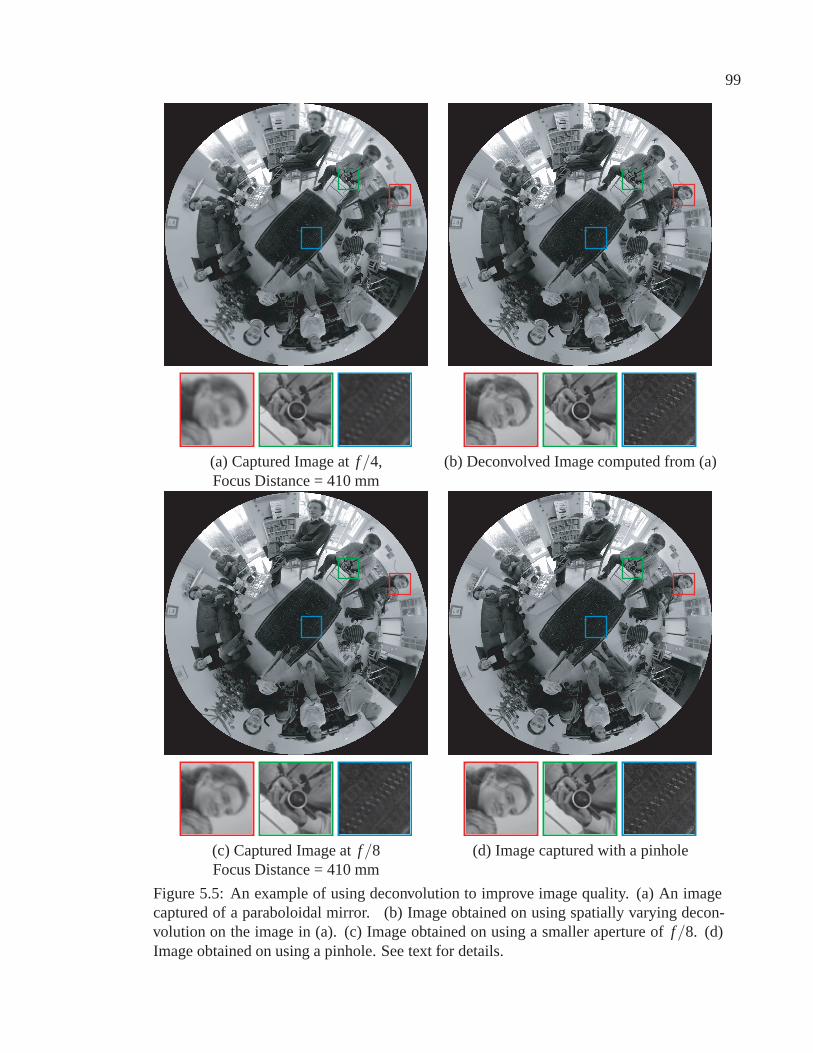
99

(a) Captured Image at f/4, (b) Deconvolved Image computed from (a)Focus Distance = 410 mm

(c) Captured Image at f/8 (d) Image captured with a pinholeFocus Distance = 410 mm

Figure 5.5: An example of using deconvolution to improve image quality. (a) An imagecaptured of a paraboloidal mirror. (b) Image obtained on using spatially varying decon-volution on the image in (a). (c) Image obtained on using a smaller aperture of f/8. (d)Image obtained on using a pinhole. See text for details.

100

(a) Captured Image at f/5.6, (b) Deconvolved Image computed from (a)Focus Distance = 412 mm

(c) Captured Image at f/11 (d) Image captured with a pinholeFocus Distance = 412 mm

Figure 5.6: An example of using deconvolution to improve image quality. (a) An imagecaptured of a spherical mirror. (b) Image obtained on using spatially varying deconvo-lution on the image in (a). (c) Image obtained on using a smaller aperture of f/11. (d)Image obtained on using a pinhole. See text for details.

101

length of 30 mm, operating at f/5.6 and was focused at a distance of 412 mm. This focus

distance was obtained from Table 5.2. The captured images had low random zero mean

Gaussian noise of 0.1%.

5.7 Discussion

In this chapter, we have shown how we can use spatially varying deconvolution to improve

the quality of images captured by imaging systems that use curved mirrors. We have shown

that at low noise levels, in some cases, deconvolution can enable us to stop-up the lens by

about 2 f-stops. This can be a significant improvement especially when capturing dimly

lit scenes. However, at moderate or high noise levels, the improvement is not as much and

deconvolution can create unacceptable artifacts.

One of the reasons why deconvolution does not produce a bigger improvement in im-

age quality is the form of the PSFs. Since we assumed a normal circular aperture, the PSFs

are usually elliptical in shape and so attenuate a lot of frequencies. One approach to rem-

edy this would be to use coded apertures [100, 190]. Using such apertures, we can control

the forms of the PSFs and manipulate them in order to preserve more higher frequencies

so that deconvolution can work well. Admittedly, some light would be lost/attenuated

because of the coded aperture, but we believe this approach can be used to realize more

invertible PSFs and hence yield greater benefits.

Finally, the approach of using deconvolution to improve the quality of images can be-

come an integral part of designing imaging systems with curved mirrors – systems can be

designed with the aim of using deconvolution to stop-up the lens. Current deconvolution

methods sometimes produce unacceptable ringing artifacts in the images. However, by

engineering invertible PSFs as well as developing more sophisticated deconvolution algo-

rithms [173, 201], approaches that leverage deconvolution can soon become mainstream.

Chapter 6

Flexible Depth of Field

The depth of field (DOF) of an imaging system is the range of scene depths that appear

focused in an image1. In virtually all applications of imaging, ranging from consumer

photography to optical microscopy, it is desirable to control the DOF. Of particular interest

is the ability to capture scenes with very large DOFs. DOF can be increased by making

the aperture smaller. However, this reduces the amount of light received by the detector,

resulting in greater image noise (lower SNR). This trade-off gets worse with decrease in

pixel size. As pixels get smaller, DOF decreases since the defocus blur occupies a greater

number of pixels. At the same time, each pixel receives less light and hence SNR falls

as well. This trade-off between DOF and SNR is one of the fundamental, long-standing

limitations of imaging.

In a conventional camera, for any location of the image detector, there is one scene

plane – the focal plane – that is perfectly focused. In this chapter, we propose varying

the position and/or orientation of the image detector during the integration time of a pho-

tograph. As a result, the focal plane is swept through a volume of the scene causing all

points within it to come into and go out of focus, while the detector collects photons.

We demonstrate that such an imaging system enables one to control the DOF in new

1The work presented in this chapter appeared at the European Conference on Computer Vision, 2008.This is joint work with Hajime Nagahara, Changyin Zhou and Shree K. Nayar.

102

103

and powerful ways:

• Extended Depth of Field: Consider the case where a detector with a global shutter (all

pixels are exposed simultaneously and for the same duration) is moved with uniform speed

during image integration. Then, each scene point is captured under a continuous range of

focus settings, including perfect focus. We analyze the resulting defocus blur kernel and

show that it is nearly constant over the range of depths that the focal plane sweeps through

during detector motion. Consequently, irrespective of the complexity of the scene, the

captured image can be deconvolved with a single, known blur kernel to recover an image

with significantly greater DOF. This approach is similar in spirit to Hausler’s work in

microscopy [72]. He showed that the DOF of an optical microscope can be enhanced by

moving a specimen of depth range d, a distance 2d along the optical axis of the microscope,

while filming the specimen. The defocus of the resulting captured image is similar over

the entire depth range of the specimen. However, this approach of moving the scene with

respect to the imaging system is practical only in microscopy and not suitable for general

scenes. More importantly, Hausler’s derivation assumes that defocus blur varies linearly

with scene depth which is true only for imaging systems that are telecentric on the object

side such as microscopes.

• Discontinuous Depth of Field: A conventional camera’s DOF is a single fronto-parallel

slab located around the focal plane. We show that by moving a global-shutter detector non-

uniformly, we can capture images that are focused for certain specified scene depths, but

defocused for in-between scene regions. Consider a scene that includes a person in the

foreground, a landscape in the background, and a dirty window in between the two. By

focusing the detector on the nearby person for some duration and the far away landscape

for the rest of the integration time, we get an image in which both appear fairly well-

focused, while the dirty window is blurred out and hence optically erased.

• Tilted Depth of Field: Most cameras can only focus on a fronto-parallel plane. An ex-

ception is the view camera configuration [112, 91], where the image detector is tilted with

104

respect to the lens. When this is done, the focal plane is tilted according to the well-known

Scheimpflug condition [169]. We show that by uniformly translating an image detector

with a rolling electronic shutter (different rows are exposed at different time intervals but

for the same duration), we emulate a tilted image detector. As a result, we capture an

image with a tilted focal plane and hence a tilted DOF.

• Non-planar Depth of Field: In traditional cameras, the focal surface is a plane. In

some applications it might be useful to have a curved/non-planar scene surface in focus.

We show that by non-uniformly (with varying speed) translating an image detector with a

rolling shutter we emulate a non-planar image detector. Consequently, we get a non-planar

focal surface and hence a non-planar DOF.

An important feature of our approach is that the focal plane of the camera can be swept

through a large range of scene depths with a very small translation of the image detector.

For instance, with a 12.5 mm focal length lens, to sweep the focal plane from a distance of

450 mm from the lens to infinity, the detector has to be translated only about 360 microns.

Since a detector only weighs a few milligrams, a variety of micro-actuators (solenoids,

piezoelectric stacks, ultrasonic transducers, DC motors) can be used to move it over the

required distance within very short integration times (less than a millisecond if required).

Note that such micro-actuators are already used in most consumer cameras for focus and

aperture control and for lens stabilization. We present several results that demonstrate the

flexibility of our system to control DOF in unusual ways. We believe our approach can

open up a new creative dimension in photography and lead to new capabilities in scientific

imaging, computer vision, and computer graphics.

6.1 Related Work

A promising approach to extended DOF imaging is wavefront coding, where phase plates

placed at the aperture of the lens cause scene objects within a certain depth range to be

105

defocused in the same way [34, 47, 19]. Thus, by deconvolving the captured image with

a single blur kernel, one can obtain an all-focused image. In this case, the effective DOF

is determined by the phase plate used and is fixed. On the other hand, in our system, the

DOF can be chosen by controlling the motion of the detector. Our approach has greater

flexibility as it can even be used to achieve discontinuous or tilted DOFs.

Recently, Levin et al. [100] and Veeraraghavan et al. [190] have used masks at the

lens aperture to control the properties of the defocus blur kernel. From a single captured

photograph, they aim to estimate the structure of the scene and then use the correspond-

ing depth-dependent blur kernels to deconvolve the image and get an all-focused image.

However, they assume simple layered scenes and their depth recovery is not robust. In

contrast, our approach is not geared towards depth recovery, but can significantly extend

DOF irrespective of scene complexity. Also, the masks used in both these previous works

attenuate some of the light entering the lens, while our system operates with a clear and

wide aperture. All-focused images can also be computed from an image captured using

integral photography [1, 137, 48]. However, since these cameras make spatio-angular res-

olution trade-offs to capture 4D lightfields in a single image, the computed images have

much lower spatial resolution when compared to our approach.

A related approach is to capture many images to form a focal stack [28, 123, 178, 7,

30, 69]. An all-in-focus image as well as scene depth can be computed from a focal stack.

However, the need to acquire multiple images increases the total capture time making the

method suitable for only quasi-static scenes. An alternative is to use very small exposures

for the individual images. However, in addition to the practical problems involved in read-

ing out the many images quickly, this approach would result in under-exposed and noisy

images that are unsuitable for depth recovery. Recently, Hasinoff and Kutulakos [71]

have proposed a technique to efficiently capture a focal stack that spans the desired DOF,

with as few images as possible, using a combination of different apertures and focal plane

locations. The individual well-exposed photographs are then composited together using a

106

variant of the Photomontage method [3] to create a large DOF composite. As a by-product,

they also get a coarse depth map of the scene. Our approach does not recover scene depth,

but can produce an all-in-focus photograph from a single, well-exposed image.

There is a previous work on moving the detector during image integration [99]. How-

ever, their focus is on handling motion blur, for which they propose to move the detector

perpendicular to the optical axis. Some previous works have also varied the orientation

or location of the image detector. Krishnan and Ahuja [91] tilt the detector and capture

a panoramic image sequence, from which they compute an all-focused panorama and a

depth map. For video super-resolution, Ben-Ezra et al. [11] capture a video sequence by

instantaneously shifting the detector within the image plane, in between the integration

periods of successive video frames.

Recently, it has been shown that a detector with a rolling shutter can be used to estimate

the pose and velocity of a fast moving object [6]. We show how a rolling shutter detector

can be used to focus on tilted scene planes as well as non-planar scene surfaces.

6.2 Camera with Programmable Depth of Field

Consider Figure 6.1(a), where the detector is at a distance v from a lens with focal length

f and an aperture of diameter a. A scene point M is imaged in perfect focus at m, if its

distance u from the lens satisfies the Gaussian lens law:

1f

=1u

+1v. (6.1)

As shown in the figure, if the detector is shifted to a distance p from the lens (dotted line),

M is imaged as a blurred circle (the circle of confusion) centered around m′. The diameter

b of this circle is given by

b =av|(v− p)| . (6.2)

107

M

m m

Aperture

v

p

u

Scene Point

b

Scene

Integration Time

Lens Detector Motion

(a) (b)

Figure 6.1: (a) A scene point M, at a distance u from the lens, is imaged in perfect focusby a detector at a distance v from the lens. If the detector is shifted to a distance p from thelens, M is imaged as a blurred circle with diameter b centered around m′. (b) Our flexibleDOF camera translates the detector along the optical axis during the integration time of animage. By controlling the starting position, speed, and acceleration of the detector, we canmanipulate the DOF in powerful ways.

The distribution of light energy within the blur circle is referred to as the point spread

function (PSF). The PSF can be denoted as P(r,u, p), where r is the distance of an image

point from the center m′ of the blur circle. An idealized model for characterizing the PSF

is the pillbox function:

P(r,u, p) =4

πb2 Π(rb), (6.3)

where, Π(x) is the rectangle function, which has a value 1, if |x|< 1/2 and 0 otherwise. In

the presence of optical aberrations, the PSF deviates from the pillbox function and is then

often modeled as a Gaussian function:

P(r,u, p) =2

π(gb)2 exp(− 2r2

(gb)2 ), (6.4)

where g is a constant.

We now analyze the effect of moving the detector during an image’s integration time.

For simplicity, consider the case where the detector is translated along the optical axis, as

in Figure 6.1(b). Let p(t) denote the detector’s distance from the lens as a function of time.

108

Lens Translation

Micro-actuator

Image Detector

Figure 6.2: Our prototype system with flexible DOF. The micro-actuator translates thedetector along the optical axis during the integration time of a single photograph.

Then the aggregate PSF for a scene point at a distance u from the lens, referred to as the

integrated PSF (IPSF), is given by

IP(r,u) =∫ T

0P(r,u, p(t)) dt, (6.5)

where T is the total integration time. By programming the detector motion p(t) – its

starting position, speed, and acceleration – we can change the properties of the resulting

IPSF. This corresponds to sweeping the focal plane through the scene in different ways.

The above analysis only considers the translation of the detector along the optical axis (as

implemented in our prototype camera). However, this analysis can be easily extended to

more general detector motions, where both its position and orientation are varied during

image integration.

Figure 6.2 shows our flexible DOF camera. It consists of a 1/3” Sony CCD (with

1024x768 pixels) mounted on a Physik Instrumente M-111.1DG translation stage. This

stage has a DC motor actuator that can translate the detector through a 15 mm range at

a top speed of 2.7 mm/sec and can position it with an accuracy of 0.05 microns. The

translation direction is along the optical axis of the lens. The CCD shown has a global

shutter and was used to implement extended DOF and discontinuous DOF. For realizing

109

Lens Scene Required MaximumFocal Depth Detector Change in

Length Range Translation Image Position1m - ∞ 81.7 µm 4.5 pixels

9.0mm .5m - ∞ 164.9 µm 5.0 pixels.2m - 0.5m 259.1 µm 7.2 pixels

1m - ∞ 158.2 µm 3.6 pixels12.5mm .5m - ∞ 320.5 µm 5.6 pixels

.2m - 0.5m 512.8 µm 8.5 pixels

Table 6.1: Translation of the detector required for sweeping the focal plane through dif-ferent scene depth ranges. As we can see, the detector has to be moved by very smalldistances to sweep very large depth ranges. The maximum change in the image positionof a scene point that results from this translation, when a 1024x768 pixel detector is used,is also shown.

tilted and non-planar DOFs, we used a 1/2.5” Micron CMOS detector (with 2592x1944

pixels) which has a rolling shutter.

Table 6.1 shows detector translations (third column) required to sweep the focal plane

through various depth ranges (second column), using lenses with two different focal lengths

(first column). As we can see, the detector has to be moved by very small distances to

sweep very large depth ranges. Using commercially available micro-actuators, such trans-

lations are easily achieved within typical image integration times (a few milliseconds to a

few seconds).

It must be noted that when the detector is translated, the magnification of the imaging

system changes2. The fourth column of Table 6.1 lists the maximum change in the image

position of a scene point for different translations of a 1024x768 pixel detector. For the

detector motions we require, the changes in magnification are very small. This does result

in the images not being perspectively correct, but the distortions are imperceptible. More

importantly, the IPSFs are not significantly affected by such a magnification change, since

a scene point will be in high focus only for a small fraction of this change and will be

2Magnification is defined as the ratio of the distance between the lens and the detector and the distancebetween the lens and the object. By translating the detector we are changing the distance between the lensand the detector, and hence changing the magnification of the system during image integration.

110

highly blurred over the rest of it. We verify this in the next section.

6.3 Extended Depth of Field (EDOF)

In this section, we show that we can capture scenes with EDOF by translating a detector

with a global shutter at a constant speed during image integration. We first show that the

IPSF for an EDOF camera is nearly invariant to scene depth for all depths swept by the

focal plane. As a result, we can deconvolve a captured image with the IPSF to obtain an

image with EDOF and high SNR.

6.3.1 Depth Invariance of IPSF

Consider a detector translating along the optical axis with constant speed s, i.e., p(t) =

p(0)+st. If we assume that the PSF of the lens can be modeled using the pillbox function

in Equation 6.3, the IPSF in Equation 6.5 simplifies to

IP(r,u) =u f

(u− f )πasT

(λ0 +λT

r− 2λ0

b(0)− 2λT

b(T )

), (6.6)

where, b(t) is the blur circle diameter at time t, and λt = 1 if b(t) ≥ 2r and 0 otherwise.

On the other hand, if we use the Gaussian function in Equation 6.4 for the lens PSF, we

get

IP(r,u) =u f

(u− f )√

2πrasT

(erfc

(r√

2gb(0)

)+ erfc

(r√

2gb(T )

)). (6.7)

Figures 6.3(a) and (c) show 1D profiles of a normal camera’s PSFs for 5 scene points with

depths between 450 and 2000 mm from a lens with focal length f = 12.5 mm and f/# =

1.4, computed using Equations 6.3 and 6.4 (with g = 1), respectively. In this simulation,

the normal camera was focused at a distance of 750 mm. Figures 6.3(b) and (d) show

111

-10 0 100

0.0040.0080.0129.9961.000

2000mm450mm

550mm1100mm

750mm

-10 0 100

0.02

0.04

0.06

0.08 2000mm450mm550mm

1100mm750mm

(a) Normal Camera (b) EDOF CameraPSF (Pillbox) IPSF

-10 0 100

0.004

0.0089.996

1.000

2000mm450mm

550mm1100mm

750mm

-10 0 100

0.02

0.04

0.06 2000mm450mm550mm

1100mm750mm

(c) Normal Camera (d) EDOF CameraPSF (Gaussian) IPSF

Figure 6.3: Simulated (a,c) normal camera PSFs and (b,d) EDOF camera IPSFs, obtainedusing pillbox and Gaussian lens PSF models for 5 scene depths. Note that the normalcamera’s PSFs vary widely with scene depth, while the EDOF cameras’s IPSFs are almostinvariant to scene depth.

the corresponding IPSFs of an EDOF camera with the same lens, p(0) = 12.5 mm, s =

1 mm/sec, and T = 0.36 sec, computed using Equations 6.6 and 6.7, respectively. As

expected, the normal camera’s PSF varies dramatically with scene depth. In contrast, the

IPSFs of the EDOF camera derived using both pillbox and Gaussian PSF models look

almost identical for all 5 scene depths, i.e., the IPSFs are depth invariant. This invariance

of the IPSF of our EDOF camera to depth is a remarkable property. As we will see shortly,

it enables us to robustly recover an EDOF image from a captured one.

To verify this empirical observation, we measured a normal camera’s PSFs and the

EDOF camera’s IPSFs for several scene depths, by capturing images of small dots placed

112

-10 0 100

0.02

0.04

-10 0 100

0.02

0.04

-10 0 100

0.02

0.04

-10 0 100

0.02

0.04

-10 0 100

0.02

0.04

-10 0 100

0.02

0.04

-10 0 100

0.02

0.04

-10 0 100

0.02

0.04

-10 0 100

0.02

0.04

0

0.02

0.04

-10 0 100

0.02

0.04

-10 0 100

0.02

0.04

-10 0 100

0.02

0.04

-10 0 100

0.02

0.04

0

0.02

0.04

EDOF Camera IPSF

Image Location (x,y)

-10 0 100

0.02

0.04

0

0.02

0.04

0

0.02

0.04

-10 0 100

0.02

0.04

-10 0 100

0.02

0.04

Normal Camera PSF

450m

m20

00m

mSc

ene

Dep

th

(0,0) pix. (212,0) pix. (424,0) pix.CenterCenter

(0,0) pix.

50x

50x55

0mm

750m

m11

00m

m

-10 0 10 -10 0 10

-10 0 10

-10 0 10

Figure 6.4: (Left column) The measured PSF of a normal camera shown for 5 different

scene depths. Note that the scale of the plot in the center row is 50 times that of the other

plots. (Right columns) The measured IPSF of our EDOF camera shown for different scene

depths (vertical axis) and image locations (horizontal axis). While a normal camera’s PSFs

vary widely with scene depth, the EDOF camera’s IPSFs are almost invariant to both scene

depth and image location.

at different depths. Both cameras have f = 12.5 mm, f/# = 1.4, and T = 0.36 sec. The de-

tector motion parameters for the EDOF camera are p(0)= 12.5 mm and s = 1 mm/sec. The

first column of Figure 6.4 shows the measured PSF at the center pixel of the normal camera

for 5 different scene depths; the camera was focused at a distance of 750 mm. (Note that

113

450

550

750

1100

2000

450

550

750

1100

2000

[mm] 450

550

750

1100

2000

450

550

750

1100

2000

[mm] (0,0

)

(106,0

)

(212,0

)

(318,0

)

(424,0

)

(0,0)

(106,0)

(212,0)

(318,0)

(424,0)

[pixels] 6

4

2

x104

(a) (b) (c)

Figure 6.5: (a) Pair-wise dissimilarity of a normal camera’s measured PSFs at the centerpixel for 5 scene depths. The camera was focused at a distance of 750 mm. (b) Pair-wise dissimilarity of the EDOF camera’s measured IPSFs at the center pixel for 5 scenedepths. (c) Pair-wise dissimilarity of the EDOF camera’s measured IPSFs at 5 differentimage locations along the center row of the image, for scene points at a distance of 750mm. (0,0) denotes the center of the image.

the scale of the plot in the center row is 50 times that of the other plots.) Columns 2-4 of

the figure show the IPSFs of the EDOF camera for 5 different scene depths and 3 different

image locations. We can see that, while the normal camera’s PSFs vary widely with scene

depth, the EDOF camera’s IPSFs appear almost invariant to both scene depth and spatial

location. This also validates our claim that the small magnification changes that arise due

to detector motion (discussed in Section 6.3.1) do not have a significant impact on the

IPSFs.

In order to quantitatively analyze the depth and space invariance of the IPSF, we use

a dissimilarity measure that accounts for the fact that in natural images all frequencies do

not have the same importance. We define the dissimilarity of two PSFs (or IPSFs) k1 and

k2 as

d(k1,k2) = ∑ω

(|K1(ω)−K2(ω)|2

|K1(ω)|2 + ε+

|K1(ω)−K2(ω)|2|K2(ω)|2 + ε

) |F(ω)|2, (6.8)

where, Ki is the Fourier transform of ki, ω represents 2D frequency, |F|2 is a weighting

term that encodes the power fall-off of Fourier coefficients in natural images [43], and ε

is a small positive constant that ensures that the denominator terms are non-zero. Figure

114

6.5(a) shows a visualization of the pair-wise dissimilarity between the normal camera’s

PSFs measured at the center pixel, for 5 different scene depths. Figure 6.5(b) shows a

similar plot for the EDOF camera’s IPSFs measured at the center pixel, while Figure 6.5(c)

shows the pair-wise dissimilarity of the IPSFs at 5 different image locations but for the

same scene depth. These plots further illustrate the invariance of an EDOF camera’s IPSF.

Furthermore, this invariance holds true for the entire range of depths swept by the focal

plane during image integration.

6.3.2 Computing EDOF Images using Deconvolution

Since the EDOF camera’s IPSF is invariant to scene depth and image location, we can

deconvolve a captured image with a single IPSF to get an image with greater DOF. A

number of techniques have been proposed for deconvolution, Richardson-Lucy and Wiener

[85] being two popular ones. For our results, we have used the approach of Dabov et

al. [26], which combines Wiener deconvolution and block-based denoising. In all our

experiments, we used the IPSF shown in the first row and second column of Figure 6.4 for

deconvolution.

Figures 6.6(a), 6.8(a), and 6.9(a) show images captured by our EDOF camera. They

were captured with a 12.5 mm Fujinon lens with f/1.4 and 0.36 second exposures. Notice

that the captured images look slightly blurry, but high frequencies of all scene elements

are captured. These scenes span a depth range of approximately 450 mm to 2000 mm

– 10 times larger than the DOF of a normal camera with identical lens settings. Figures

6.6(b), 6.8(b), and 6.9(b) show the EDOF images computed from the captured images, in

which all scene elements appear focused3. Figures 6.7(a), 6.8(c), and 6.9(c) show images

captured by a normal camera with the same f/# and exposure time. The nearest scene

elements are in focus, while, as expected, the farther scene elements are severely blurred.

We can get a large DOF image using a smaller aperture. Images captured by a normal

3Mild ringing artifacts in the computed EDOF images are due to deconvolution.

115

Please zoom in to see noise and defocus blur

(a) Captured Image ( f/1.4, T = 0.36 sec)

(b) Computed EDOF Image

Figure 6.6: (a) Image captured by our EDOF camera. (b) EDOF image computed fromimage in (a). Note that the entire scene appears focused.

camera with the same exposure time, but with a smaller aperture of f/8 are shown in

Figures 6.7(b), 6.8(d), and 6.9(d). The intensities of these images were scaled up so that

their dynamic range matches that of the corresponding computed EDOF images. All scene

elements look reasonably sharp, but the images are very noisy as can be seen in the insets

116

Please zoom in to see noise and defocus blur

(a) Image from Normal Camera ( f/1.4, T = 0.36 sec, Near Focus)

(b) Image from Normal Camera ( f/8, T = 0.36 sec, Near Focus) with Scaling

Figure 6.7: (a) Image captured by a normal camera with identical settings as the image inFigure 6.6(a), with the nearest object in focus. (b) Image captured by a normal camera atf/8. The image intensities were scaled to match the dynamic range of the EDOF imagein Figure 6.6(b). All scene elements look reasonably sharp, but this image is much noisierthan the EDOF one in Figure 6.6(b), as exemplified by the magnified inset.

(zoomed). The computed EDOF images have much less noise, while having comparable

sharpness, i.e. our EDOF camera can capture scenes with large DOFs as well as high SNR.

117

Please zoom in to see noise and defocus blur

(a) Captured Image ( f/1.4, T = 0.36 sec) (b) Computed EDOF Image

(c) Image from Normal Camera (d) Image from Normal Camera( f/1.4, T = 0.36 sec, Near Focus) ( f/8, T = 0.36 sec, Near Focus) with Scaling

Figure 6.8: (a) Image captured by our EDOF camera. (b) EDOF image computed fromimage in (a). Note that the entire scene appears focused. (c) Image captured by a normalcamera with identical settings, with the nearest object in focus. (d) Image captured by anormal camera at f/8. The image intensities were scaled to match the dynamic range ofthe image in (b). All scene elements look reasonably sharp, but this image is much noisierthan the EDOF one in (b), as exemplified by the magnified inset.

Figure 6.10 shows another example, of a scene captured outdoors at night. As we can see,

in a normal camera, the tradeoff between DOF and SNR is extreme for such dimly lit

scenes. Our EDOF camera operating with a large aperture is able to capture something in

this scene, while a normal camera with a comparable DOF is too noisy to be useful. High

resolution versions of these images as well as other examples can be seen at [140].

Since we translate the detector at a constant speed, the IPSF does not depend on the

118

Please zoom in to see noise and defocus blur

(a) Captured Image ( f/1.4, T = 0.36 sec) (b) Computed EDOF Image

(c) Image from Normal Camera (d) Image from Normal Camera( f/1.4, T = 0.36 sec, Near Focus) ( f/8, T = 0.36 sec, Near Focus) with Scaling

Figure 6.9: (a) Image captured by our EDOF camera. (b) EDOF image computed fromimage in (a). Note that the entire scene appears focused. (c) Image captured by a normalcamera with identical settings, with the nearest object in focus. (d) Image captured by anormal camera at f/8. The image intensities were scaled to match the dynamic range ofthe image in (b). All scene elements look reasonably sharp, but this image is much noisierthan the EDOF one in (b).

direction of motion – it is the same whether the detector moves from a distance a from the

lens to a distance b from the lens or from a distance b from the lens to a distance a from the

lens. We can exploit this to get EDOF video by moving the detector alternately forward

one frame and backward the next. Figure 6.11(a) shows a frame from a video sequence

captured in this fashion and Figure 6.11(b) shows the EDOF frame computed from it. For

comparison, Figures 6.11(c) and (d) show frames from video sequences captured by a

119

Please zoom in to see noise and defocus blur

(a) Captured Image ( f/1.4, T = 0.72 sec) (b) Computed EDOF Image

(c) Image from Normal Camera (d) Image from Normal Camera( f/1.4, T = 0.72 sec, Near Focus) ( f/8, T = 0.72 sec, Near Focus) with Scaling

Figure 6.10: (a) Image captured by our EDOF camera outdoors at night. (b) EDOF im-age computed from image in (a). Note that the entire scene appears focused. (c) Imagecaptured by a normal camera with identical settings, with the nearest object in focus. (d)Image captured by a normal camera at f/8. This image is very noisy and almost unusable.As we can see, in a normal camera the tradeoff between DOF and SNR is extreme for suchdimly lit scenes.

normal camera operating at f/1.4 and f/8 respectively.

6.3.3 Analysis of SNR Benefits of EDOF Camera

We now analyze the SNR benefits of using our approach to capture scenes with extended

DOF. Deconvolution using Dabov et al.’s method [26] produces visually appealing results,

but since it has a non-linear denoising step, it is not suitable for analyzing the SNR of

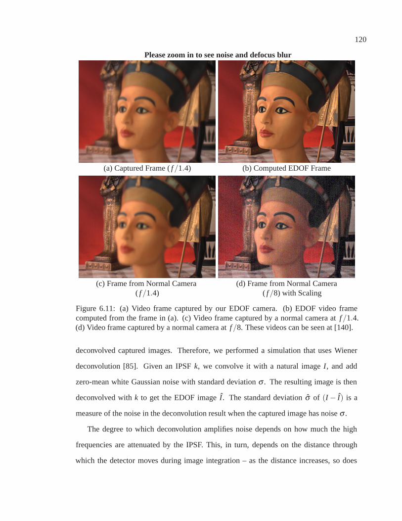
120

Please zoom in to see noise and defocus blur

(a) Captured Frame ( f/1.4) (b) Computed EDOF Frame

(c) Frame from Normal Camera (d) Frame from Normal Camera( f/1.4) ( f/8) with Scaling

Figure 6.11: (a) Video frame captured by our EDOF camera. (b) EDOF video framecomputed from the frame in (a). (c) Video frame captured by a normal camera at f/1.4.(d) Video frame captured by a normal camera at f/8. These videos can be seen at [140].

deconvolved captured images. Therefore, we performed a simulation that uses Wiener

deconvolution [85]. Given an IPSF k, we convolve it with a natural image I, and add

zero-mean white Gaussian noise with standard deviation σ . The resulting image is then

deconvolved with k to get the EDOF image I. The standard deviation σ of (I − I) is a

measure of the noise in the deconvolution result when the captured image has noise σ .

The degree to which deconvolution amplifies noise depends on how much the high

frequencies are attenuated by the IPSF. This, in turn, depends on the distance through

which the detector moves during image integration – as the distance increases, so does

121

the attenuation of high frequencies. This is illustrated in Figure 6.12(a), which shows

(in red) the MTF (magnitude of the Fourier transform) for a simulated IPSF k1, derived

using the pillbox lens PSF model. In this case, we use the same detector translation (and

other parameters) as in our EDOF experiments (Section 6.3.1). The MTF of the IPSF k2

obtained when the detector translation is halved (keeping the mid-point of the translation

the same) is also shown (in blue). As expected, k2 attenuates the high frequencies less than

k1.

We analyzed the SNR benefits for these two IPSFs for different noise levels in the

captured image. The table in Figure 6.12(b) shows the noise produced by a normal camera

for different aperture sizes, given the noise level for the largest aperture, f/1.4. (Image

brightness is assumed to lie between 0 and 1.) The last two rows show the effective noise

levels for EDOF cameras with IPSFs k1 and k2, respectively. The last column of the table

shows the effective DOFs realized; the normal camera is assumed to be focused at a scene

distance that corresponds to the center position of the detector motion. One can see that,

as the noise level in the captured image increases, the SNR benefits of EDOF cameras

increase. As an example, if the noise of a normal camera at f/1.4 is 0.01, then the EDOF

camera with IPSF k1 has the SNR of a normal camera operating at f/2.8, but has a DOF

that is greater than that of a normal camera at f/8.

In the above analysis, the SNR was averaged over all frequencies. However, it must

be noted that SNR is frequency dependent - SNR is greater for lower frequencies than

for higher frequencies in the deconvolved EDOF images. Hence, high frequencies in an

EDOF image would be degraded, compared to the high frequencies in a perfectly focused

image. However, in our experiments this degradation is not strong, as can be seen in the

insets of Figures 6.8(b) and (c) and the full resolution images at [140].

Different frequencies in the image having different SNRs illustrates the tradeoff that

our EDOF camera makes. In the presence of noise, instead of capturing with high fidelity,

high frequencies over a small range of scene depths (the depth of field of a normal camera),

122

0

0.2

0.4

0.6

0.8

1.0

1.00.80.60.40.20

IPSF k1IPSF k 2

MTF

Spatial frequency [cycle/pixel]

(a)Camera f/# Noise standard deviation DOF (mm)Normal 1.4 0.001 0.002 0.005 0.010 0.020 140.98Normal 2.8 0.004 0.008 0.020 0.040 0.080 289.57Normal 4 0.008 0.016 0.041 0.082 0.163 429.77Normal 5.6 0.016 0.032 0.080 0.160 0.320 649.21Normal 8 0.033 0.065 0.163 0.327 0.653 1114.56

EDOF(k1) 1.4 0.013 0.021 0.036 0.049 0.062 1622.44EDOF(k2) 1.4 0.0073 0.0133 0.0262 0.0399 0.0570 528.56

(b)

Figure 6.12: (a) MTFs of simulated IPSFs, k1 and k2, of an EDOF camera correspondingto the detector traveling two different distances during image integration. (b) Comparisonof effective noise and DOF of a normal camera and a EDOF camera with IPSFs k1 and k2.The image noise of a normal camera operating at f/1.4 is assumed to be known.

our EDOF camera captures with slightly lower fidelity, high frequencies over a large range

of scene depths.

6.4 Discontinuous Depth of Field

Consider the image in Figure 6.13(a), which shows two toys (cow and hen) in front of a

scenic backdrop with a wire mesh in between. A normal camera with a small DOF can

capture either the toys or the backdrop in focus, while eliminating the mesh via defocusing.

However, since its DOF is a single continuous volume, it cannot capture both the toys and

the backdrop in focus and at the same time eliminate the mesh. If we use a large aperture

and program our camera’s detector motion such that it first focuses on the toys for a part of

the integration time, and then moves quickly to another location to focus on the backdrop

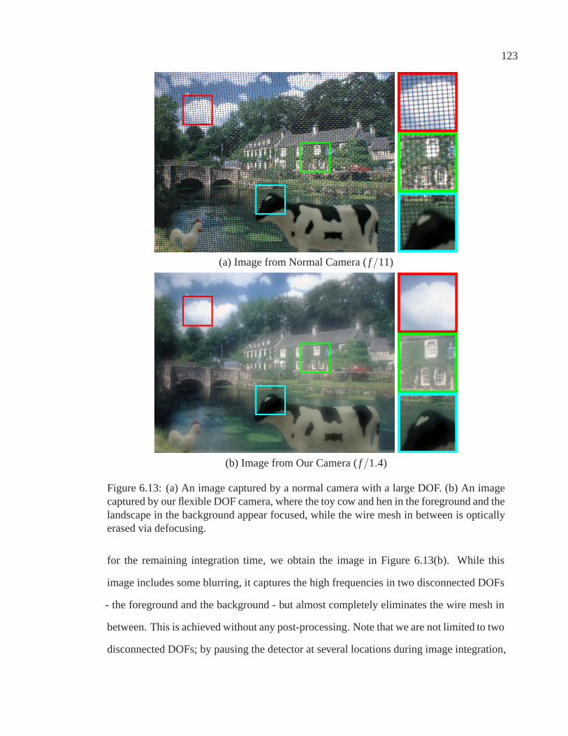
123

(a) Image from Normal Camera ( f/11)

(b) Image from Our Camera ( f/1.4)

Figure 6.13: (a) An image captured by a normal camera with a large DOF. (b) An imagecaptured by our flexible DOF camera, where the toy cow and hen in the foreground and thelandscape in the background appear focused, while the wire mesh in between is opticallyerased via defocusing.

for the remaining integration time, we obtain the image in Figure 6.13(b). While this

image includes some blurring, it captures the high frequencies in two disconnected DOFs

- the foreground and the background - but almost completely eliminates the wire mesh in

between. This is achieved without any post-processing. Note that we are not limited to two

disconnected DOFs; by pausing the detector at several locations during image integration,

124

more complex DOFs can be realized.

6.5 Tilted Depth of Field

Normal cameras can focus on only fronto-parallel scene planes. On the other hand, view

cameras [112, 91] can be made to focus on tilted scene planes by adjusting the orientation

of the lens with respect to the detector. We show that our flexible DOF camera can be

programmed to focus on tilted scene planes by simply translating (as in the previous appli-

cations) a detector with a rolling electronic shutter. A large fraction of CMOS detectors

are of this type – while all pixels have the same integration time, successive rows of pixels

are exposed with a slight time lag. If the exposure time is sufficiently small, then upto an

approximation, we can say that the different rows of the image are exposed independently.

When such a detector is translated with uniform speed s, during the frame read out time T

of an image, we emulate a tilted image detector. If this tilted detector makes an angle θ

with the lens plane, then the focal plane in the scene makes an angle φ with the lens plane,

where θ and φ are related by the well-known Scheimpflug condition [169]:

θ = tan−1(sTH

) and, φ = tan−1(

2 f tan(θ)2p(0)+H tan(θ)−2 f

). (6.9)

Here, H is the height of the detector. Therefore, by controlling the speed s of the detector,

we can vary the tilt angle of the image detector, and hence the tilt of the focal plane and its

associated DOF.

Figure 6.14 shows a scene where the dominant scene plane – a table top with a news-

paper, keys and a mug on it – is inclined at an angle of approximately 53 with the lens

plane. As a result, a normal camera is unable to focus on the entire plane, as seen in Fig-

ure 6.14(a). By translating a rolling-shutter detector (1/2.5” CMOS sensor with a 70 msec

exposure lag between the first and last row of pixels) at 2.7 mm/sec, we emulate a detector

125

(a) Image from Normal Camera ( f/1.4, T = 0.03 sec)

(b) Image from our Camera ( f/1.4, T = 0.03 sec)

Figure 6.14: (a) An image captured by a normal camera of a table top inclined at 53 withrespect to the lens plane. (b) An image captured by our flexible DOF camera, where theDOF is tilted by 53. The entire table top (with the newspaper and keys) appears focused.Observe that the top of the mug is defocused, but the bottom appears focused, illustratingthat the focal plane is aligned with the table top. Three scene regions of both the imagesare shown at a higher resolution to highlight the defocus effects.

tilt of 2.6. This enables us to achieve the desired DOF tilt of 53 (from Equation 6.9) and

capture the table top (with the newspaper and keys) in focus, as shown in Figure 6.14(b).

Observe that the top of the mug is not in focus, but the bottom appears focused, illustrat-

ing the fact that the DOF is tilted to be aligned with the table top. Note that there is no

126

post-processing here.

6.6 Non-Planar Depth of Field

In the previous section, we have seen that by uniformly translating a detector with a rolling

shutter we can emulate a tilted image detector. Taking this idea forward, if we translate

such a detector in some non-uniform fashion (varying speed), we can emulate a non-planar

image detector. Consequently, we get a non-planar focal surface and hence a non-planar

DOF. This is in contrast to a normal camera which has a planar focal surface and whose

DOF is a fronto-parallel slab.

Figure 6.15 (a) shows a scene captured by a normal camera. It has crayons arranged

on a semi-circle with a price tag in the middle placed at the same depth as the left-most

and right-most crayons. In this image, only the two extreme crayons on either side and

the price tag are in focus; the remaining crayons are defocused. Say, we want to capture

this scene so that the DOF is ‘curved’ – the crayons are in focus while the price tag is

defocused. We set up a non-uniform motion of the detector to achieve this desired DOF,

which can be seen in Figure 6.15 (b).

6.7 Exploit Camera’s Focusing Mechanism to Manipulate

Depth of Field

Till now we have seen that by moving the detector during image integration, we can ma-

nipulate the DOF. However, it must be noted that whatever effect we get by moving the

detector, we can get exactly the same effect by moving the lens (in the opposite direction).

In fact, cameras already have mechanisms to do this; this is what happens during focus-

ing. Hence, we can exploit the camera’s focusing mechanism to manipulate DOF. Figure

6.16(a) shows an image captured by a normal SLR camera (Canon EOS 20D with a Sigma

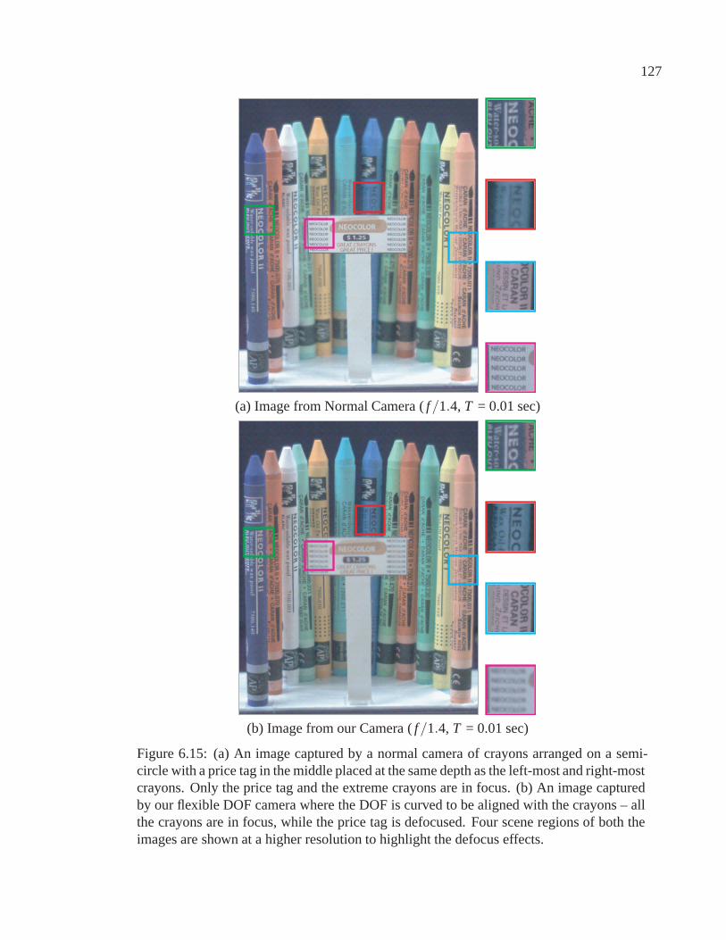
127

(a) Image from Normal Camera ( f/1.4, T = 0.01 sec)

(b) Image from our Camera ( f/1.4, T = 0.01 sec)

Figure 6.15: (a) An image captured by a normal camera of crayons arranged on a semi-circle with a price tag in the middle placed at the same depth as the left-most and right-mostcrayons. Only the price tag and the extreme crayons are in focus. (b) An image capturedby our flexible DOF camera where the DOF is curved to be aligned with the crayons – allthe crayons are in focus, while the price tag is defocused. Four scene regions of both theimages are shown at a higher resolution to highlight the defocus effects.

128

30 mm lens) at f/1.4, where only the near flowers are in focus. To capture this scene with

an extended DOF, we manually rotated the focus ring of the SLR camera lens uniformly

during image integration. For the lens we used, uniform rotation corresponds to moving

the lens at a roughly constant speed. Figure 6.16(b) shows an image captured in this fash-

ion. Figure 6.16(c) shows the EDOF image computed from it, in which the entire scene

appears sharp and well focused. Figure 6.17 shows another example. These images can

be seen at full resolution at [140].

6.8 Computing an All-Focused Image from a Focal Stack

Our approach to extended DOF also provides a convenient means to compute an all-

focused image from a focal stack. Traditionally, given a focal stack, for every pixel we

have to determine in which image that particular pixel is in-focus [17, 65]. This requires

computing at each pixel a focus measure that uses a patch of surrounding pixels as a

support4. Hence, this approach tends to have problems at occlusion boundaries. Some

previous works have tackled this as a labeling problem, where the label for every pixel is

the input photograph where the pixel is in-focus. The labels are optimized using a Markov

Random Field that is biased towards piece-wise smoothness [3, 71].

We propose an alternate approach that leverages our observations in Section 6.3.1. We

propose to compute a weighted average of all the images of the focal stack (compensating

for magnification effects if possible), where the weights are chosen to mimic changing the

distance between the lens and the detector at a constant speed. From Section 6.3.1 we

know that this average image would have depth independent blur. Hence, deconvolution

with a single blur kernel will give a sharp image in which all scene elements appear fo-

cused. Figures 6.18(a,b,c) show three of the 28 images that form a focal stack. These

were captured with a Canon 20D SLR camera with a Sigma 30 mm lens operating at

4An exception is [70] that proposes to capture a stack of images while varying both focus setting andaperture. In this scenario, a focus measure can be computed at each pixel independently.

129

(a) Image from Normal Camera ( f/1.4, T = 0.6 sec)

(b) Captured EDOF Image (c) Computed EDOF Image( f/1.4, T = 0.6 sec)

Figure 6.16: (a) Image captured by a Canon EOS 20D SLR camera with a Sigma 30 mmlens operating at f/1.4, where only the near flowers are in focus. (b) Image captured bythe camera when the focus ring was manually rotated uniformly during image integration.Uniform rotation of the focus ring corresponds to moving the lens at roughly constantspeed. (c) Image with extended DOF computed from the image in (b).

130

(a) Captured EDOF Image (b) Computed EDOF Image( f/1.4, T = 0.6 sec)

(c) Image from Normal Camera (d) Image from Normal Camera( f/1.4, T = 0.6 sec) ( f/8, T = 0.6 sec)

Figure 6.17: (a) Image captured by manually rotating the focus ring of a Sigma 30 mmlens on a Canon EOS 20D SLR camera. The lens was operating at f/1.4. (b) Image withextended DOF computed from the image in (a). (c) Image captured by a normal cameraoperating at f/1.4 where only the near flowers and leaves are in focus. (d) Image capturedby a normal camera operating at f/8. All scene elements look sharp, but the image isnoisy.

131

(a) (b)

(c) (d)

Figure 6.18: (a,b,c) Three out of 28 images that form a focal stack. The images werecaptured with a Canon 20D camera with a Sigma 30 mm lens operating at f/1.4. (d) Theall-focused image computed from the focal stack images using the approach described inSection 6.8.

f/1.4. Figure 6.18(d) shows the all-focused image computed from the focal stack using

our approach.

6.9 Discussion

In this chapter we have proposed a camera with a flexible DOF. DOF is manipulated in

various ways by controlling the motion of the detector during the exposure of a single

image. We have shown how such a system can capture arbitrarily complex scenes with

extended DOF while using large apertures. We have also shown that we can create DOFs

that span multiple disconnected volumes. In addition, we have demonstrated that our

camera can focus on tilted scene planes as well as non-planar scene surfaces. Finally, we

have shown that we can manipulate DOF by exploiting the focusing mechanism of the

132

lens. This can be very convenient and practical, especially for camera manufacturers.

Effects at Occlusion Boundaries For our EDOF camera, we have not explicitly modeled

the defocus effects at occlusion boundaries. Due to defocus blur, image points that lie

close to occlusion boundaries can receive light from scene points at very different depths.

However, since the IPSF of the EDOF camera is nearly depth invariant, the aggregate IPSF

for such an image point can be expected to be similar to the IPSF of points far from oc-

clusion boundaries. In some of our experiments, we have seen mild ringing artifacts at

occlusion boundaries. These can possibly be eliminated using more sophisticated decon-

volution algorithms such as [201, 173]. Note that in tilted and non-planar DOF examples

occlusion boundaries are correctly captured; there are no artifacts.

Effects of Scene Motion The simple off-the-shelf actuator that we used in our prototype

has low translation speeds and so we had to use exposure times of about 1/3rd of a second

to capture EDOF images. However, we have not observed any visible artifacts in EDOF

images computed for scenes with typical object motion (see Figures 6.6 and 6.8). With

faster actuators, like piezoelectric stacks, exposure times can be made much smaller and

thereby allow captured scenes to be more dynamic. However, in general, motion blur due

to high-speed objects can be expected to cause problems. In this case, a single pixel sees

multiple objects with possibly different depths and it is possible that neither of the objects

are imaged in perfect focus during detector translation. This scenario is an interesting one

that warrants further study. In tilted and non-planar DOF applications, fast moving scene

points can end up being imaged at multiple image locations. All images of a moving scene

point would be in-focus if its corresponding 3D positions lie within the (planar/non-planar)

DOF. These multiple image locations can be used to measure the velocity and pose of the

scene point, as was shown by [6].

Using Different Actuators In our prototype, we have used a simple linear actuator whose

action was synchronized with the exposure time of the detector. However, other more so-

phisticated actuators can be used. As mentioned above, faster actuators like piezoelectric

133

stacks can dramatically reduce the time needed to translate a detector over the desired dis-

tance and so enable low exposure times. This can be very useful for realizing tilted and

non-planar DOFs, which need low exposure times. In an EDOF camera, an alternative to a

linear actuator is a vibratory or oscillatory actuator – the actuator causes the detector to vi-

brate with an amplitude that spans the total desired motion of the detector. If the frequency

of the vibration is very high (around 100 times within the exposure of an image), then one

would not need any synchronization between the detector motion and the exposure time

of the detector; errors due to lack of synchronization would be negligible.

Robustness of EDOF Camera PSF In our experience, the EDOF camera’s PSF is very

robust to the actual motion of the detector or the lens. This is illustrated by the fact, that

we are able to capture scenes with large DOFs even when the motion realized is only

approximately uniform (see example in Section 6.7). Since this approach does not seem

susceptible to small errors in motion, it is particularly attractive for practical implementa-

tion in cameras.

Realizing Arbitrary DOFs We have shown how we can exploit rolling shutter detectors

to realize tilted and non-planar DOFs (Sections 6.5 and 6.6). In these detectors if the

exposure time is sufficiently small, then we can approximately say that the different rows

of the image are exposed independently. This allows us to realize DOFs where the focal

surfaces are swept surfaces. It is conceivable, that in the future we might have detectors

that provide pixel level control of exposure – we can independently control the start and

end time of the exposure of each pixel. Such control coupled with a suitable detector

motion would enable us to independently choose the scene depth that is imaged in-focus

at every pixel, yielding arbitrary DOF manifolds.

Practical Implementation All DOF manipulations shown in this paper can be realized by

moving the lens during image integration (Section 6.7 shows one example). Compared to

moving the detector, moving the lens would be more attractive for camera manufacturers,

since cameras already have actuators that move the lens for focusing. All that is needed

134

is to expose the detector while the focusing mechanism sweeps the focal plane through

the scene. Hence, implementing these DOF manipulations would not be difficult and can

possibly be realized by simply updating the camera firmware.

We believe that flexible DOF cameras can open up a new creative dimension in pho-

tography and lead to new capabilities in scientific imaging, computer vision, and computer

graphics. Our approach provides a simple means to realizing such flexibility.

Chapter 7

Conclusions

Computational imaging has attracted a lot of attention in recent years to capture more/better

scene information. With Moore’s law, computing power has become increasingly cheaper.

Today’s cameras do a lot of processing on chip and it is conceivable that in the near future

there will be enough computing power available on cameras for sophisticated computa-

tional imaging techniques and consequently for the widespread adoption of these tech-

niques. The fusion of new optics and devices with the principles of conventional cameras

can open up new creative dimensions in photography and at the same time provide much

desired flexibility for vision applications like surveillance.

In this thesis, we have proposed and analyzed three computational imaging systems. In

Chapter 3, we examined a family of imaging systems called radial imaging systems. These

imaging systems adopt an object-side coding strategy using reflective optics – a hollow

truncated conical mirror placed in front of a conventional camera. We have demonstrated

the flexibility of this family of systems to capture depth – from small 3D textures with

fine geometry to macroscopic objects such as faces. We have also shown how different

members of the family can be used for estimating the BRDFs of isotropic materials and

capturing complete texture maps and geometries of convex objects. For most of these

applications only a single image has to be captured.

135

136

In Chapter 4, we proposed an imaging system with a flexible field of view – the size and

shape of the field of view can be varied to achieve a desired scene composition, within a

single image. This system too adopts an object-side coding strategy using reflective optics;

it images the scene reflected in a flexible mirror sheet, which can be deformed to realize a

wide range of curved mirror shapes. This system enables a wide range of scene-to-image

mappings.

In Chapter 6, we looked at an imaging system with a flexible depth of field, which

implements a detector side coding strategy using detector motion. We proposed moving

the image detector along the optical axis during the integration time of a photograph. By

controlling the starting position, speed, and acceleration we can manipulate the depth of

field. We showed how we can capture scenes with large depths of field while using large

apertures in order to maintain high signal to noise ratio. Our flexible imaging system can

also capture scenes with discontinuous, tilted, or non-planar depths of field.

In Chapter 5, we examined a problem that afflicts all imaging systems that use curved

mirrors. Due to the use of a finite lens aperture and local mirror curvature effects, the

captured image is usually not entirely in focus. We have proposed a deconvolution based

approach to improve image quality. If the lens properties, mirror shape, and mirror location

are known, we can numerically compute the spatially varying blur due to the combined

action of the lens and the mirror. We have shown that using spatially varying deconvolution

we can computationally stop up the lens – use a larger aperture to capture an image which

after deconvolution has scene objects with the same sharpness as using a smaller aperture.

The imaging systems and algorithms presented in this thesis demonstrate the power of

computational imaging in enhancing the capabilities of cameras. The first Kodak camera

released in 1888 had the marketing slogan “You press the button, we do the rest”. The

next generation of cameras built with conventional camera principles and ideas from com-

putational imaging will potentially be marketed as “You press the button, we do a lot more

...”.

137

7.1 Future Directions

With cameras making great technological advances – increasing detector resolution, more

sensitive detectors, better lenses, faster image acquisition times, more control over capture

settings, sophisticated electronics on chip, etc. – it seems to be a great time to think about

how we can better capture scenes. Computational imaging has proven to be an attractive

approach to go beyond the principles of the camera obscura that have defined cameras.

This thesis has proposed some novel imaging systems that follow this line of thought. The

confluence of new optics and devices and the ever increasing computational power at our

disposal means that such approaches will be actively explored in the future. Here we list

some ideas related to the ones presented in this thesis.

Computational Projectors

Cameras and projectors are duals; while cameras capture scene rays, projectors project

rays into the scene. Their optical principles are identical. Therefore, it is conceivable that

computational imaging ideas can be applied to projectors. In particular, some applications

can benefit from using projectors in conjunction with curved mirrors.

In underwater imaging, the imaging system has to project light and then capture the

light reflected from the scene. For compactness, it is desirable to co-locate the camera

and the projector. However, because of backscattering due to impurities, a major portion

of the captured light might be because of scattering. One approach could be to use a

hollow conical mirror with a projector, similar to the systems in Chapter 3. A photo-

sensor is co-located with the projector. The projector is used to illuminate the scene via

the mirror. The projector and the mirror give rise to a locus or multiple loci of circular

virtual projection points (analogous to virtual viewpoints). From Section 3.4.3, if we use

the projector to project a circle, all the corresponding light rays after reflection in the mirror

would intersect and hence illuminate a single point on the optical axis. The reflected light

138

is measured by the photo-sensor. By projecting different circles, points in the volume at

different distances along the optical axis are illuminated. From the measurements we can

infer the properties of the volume along the optical axis. By translating the system, we

can scan the entire volume. This approach has two advantages. First, light rays from the

projector after reflection in the mirror, illuminate a point in the volume from the sides and

so avoid backscattering effects. Secondly, since light rays from multiple projector pixels

are used to illuminate a single point in the volume (there is more light), the measurements

are less noisy than using only the projector.

Depth from Defocus using Detector Motion

In many applications, it would be desirable to capture both an all-focused image as well

as get 3D scene structure. Depth from defocus uses two images captured with different

focus settings to recover 3D structure. However, the captured images are usually not

suitable for computing an all-focused image because of the loss of high frequencies due

to blurring. One approach could be to capture two images – the first is an image captured

as in conventional depth from defocus and the second is an all-focused image obtained

using our approach of moving the detector described in Chapter 6. To realize the capture

of this pair of images, one could take the first image at the starting position of the motion

of the detector and then take the second while moving the detector at a constant speed.

Comparing an image with defocus blur with the all-focused image could enable more

robust recovery of scene structure, while using large apertures to keep the acquisition

time small. The time required by cameras between photographs is decreasing and it is

conceivable that soon cameras could be equipped to capture two photographs in quick

succession on pressing the shutter button and realize applications such as these.

139

Detector Motion and Curved Mirror Defocus

In Chapter 5, we have shown that we can leverage deconvolution algorithms to improve

the quality of images captured by imaging systems with curved mirrors. However, the blur

kernels in these systems usually attenuate a lot of frequencies – just like conventional cam-

eras – and so the benefits are modest even at low noise levels. In Chapter 6 we saw that by

moving the detector we could shape the PSFs to lower the attenuation of high frequencies

and make the PSFs more invertible. Analogously, by moving the detector while imaging

the reflections of a scene in a curved mirror, the resulting PSFs might be more invertible

and consequently the benefits on using deconvolution can be more significant.

Chapter 8

Bibliography

[1] E. Adelson and J. Wang. Single lens stereo with a plenoptic camera. IEEE Transac-tions on Pattern Analysis and Machine Intelligence (PAMI), pages 99–106, 1992.

[2] H. Adorf. Towards HST Restoration with a Space-Variant PSF, Cosmic Rays andOther Missing Data. The Restoration of HST Images and Spectra II, pages 72–78,1994.

[3] A. Agarwala, M. Dontcheva, M. Agrawala, S. Drucker, A. Colburn, B. Curless,D. Salesin, and M. Cohen. Interactive digital photomontage. ACM Transactions onGraphics (SIGGRAPH), pages 294–302, 2004.

[4] M. Aggarwal and N. Ahuja. High dynamic range panoramic imaging. IEEE Inter-national Conference on Computer Vision (ICCV), pages 2–9, 2001.

[5] M. Aggarwal and N. Ahuja. Split Aperture Imaging for High Dynamic Range.International Journal of Computer Vision (IJCV), pages 7–17, 2004.

[6] Omar Ait-Aider, Nicolas Andreff, Jean-Marc Lavest, and Philippe Martinet. Simul-taneous Object Pose and Velocity Computation Using a Single View from a RollingShutter Camera. European Conference on Computer Vision (ECCV), pages 56–68,2006.

[7] K. Aizawa, K. Kodama, and A. Kubota. Producing object-based special effects byfusing multiple differently focused images. TCSVT, pages 323–330, 2000.

[8] Chadi Albitar, Pierre Graebling, and Christophe Doignon. Robust structured lightcoding for 3D reconstruction. IEEE International Conference on Computer Vision(ICCV), pages 1–6, 2007.

[9] Simon Baker and Shree K. Nayar. A Theory of Single-Viewpoint CatadioptricImage Formation. International Journal of Computer Vision (IJCV), pages 175–196, 1999.

[10] L. Bar, N. A. Sochen, and N. Kiryati. Restoration of Images with Piecewise Space-Variant Blur. SSVM07, pages 533–544, 2007.

140

141

[11] M. Ben-Ezra, A. Zomet, and S.K. Nayar. Jitter Camera: High Resolution Videofrom a Low Resolution Detector. IEEE Computer Vision and Pattern Recognition(CVPR), pages 135–142, 2004.

[12] Moshe Ben-Ezra, Zhouchen Lin, and Bennett Wilburn. Penrose Pixels Super-Resolution in the Detector Layout Domain. IEEE International Conference onComputer Vision (ICCV), pages 1–8, 2007.

[13] A. F. Boden, D. C. Redding, R. J. Hanisch, and J.Mo. Massively Parallel Spatially-Variant Maximum Likelihood Restoration of Hubble Space Telescope Imagery.Journal of the Optical Society of America, pages 1537–1545, 1996.

[14] F. L. Bookstein. Principal Warps: Thin Plate Splines and the Decomposition ofDeformations. IEEE Transactions on Pattern Analysis and Machine Intelligence(PAMI), 11:567–585, 1989.

[15] M. Born and E. Wolf. Principles of Optics. Permagon Press, 1965.

[16] V. Brajovic and T. Kanade. A Sorting Image Sensor: An Example of Massively Par-allel Intensity-to- Time Processing for Low-Latency Computational Sensors. IEEEConference on Robotics and Automation (ICRA), page 16381643, 1996.

[17] P. Burt and R. Kolczynski. Enhanced image capture through fusion. IEEE Interna-tional Conference on Computer Vision (ICCV), pages 173–182, 1993.

[18] A. Busboom, H.D. Schotten, and H. Elders-Boll. Coded aperture imaging withmultiple measurements. Journal of the Optical Society of America A: Optics, pages1058–1065, 1997.

[19] A. Castro and J. Ojeda-Castaneda. Asymmetric Phase Masks for Extended Depthof Field. Applied Optics, pages 3474–3479, 2004.

[20] W.T. Cathey and E.R. Dowski. New paradigm for imaging systems. Applied Optics,pages 6080–6092, 2002.

[21] J. Chahl and M. Srinivasan. Reflective surfaces for panoramic imaging. AppliedOptics, pages 8275–8285, 1997.

[22] M.P. Christensen, G.W. Euliss, M.J. McFadden, K.M. Coyle, P. Milojkovic, M.W.Haney, J. van der Gracht, and R. A. Athale. Active-eyes: An adaptive pixel-by-pixel image-segmentation sensor architecture for high-dynamic range hyperspectralimaging. Applied Optics, pages 6093–6103, 2002.

[23] T. Conroy and J. Moore. Resolution invariant surfaces for panoramic vision systems.IEEE International Conference on Computer Vision (ICCV), pages 392–397, 1999.

[24] R. Cook and K. Torrance. A reflectance model for computer graphics. ACM SIG-GRAPH, pages 307–316, 1981.

142

[25] Cyberware. http://www.cyberware.com/.

[26] K. Dabov, A. Foi, V. Katkovnik, and K. Egiazarian. Image restoration by sparse 3Dtransform-domain collaborative filtering. SPIE Electronic Imaging, 2008.

[27] K. Dana. BRDF/BTF Measurement Device. IEEE International Conference onComputer Vision (ICCV), pages 460–466, 2001.

[28] T. Darrell and K. Wohn. Pyramid based depth from focus. IEEE Computer Visionand Pattern Recognition (CVPR), pages 504–509, 1988.

[29] Andrew Davidhazy. Peripheral Photography: Shooting full circle. Industrial Pho-tography, 36:28–31, 1987.

[30] Ishita Deb, Bhabatosh Chandaa, and Buddhajyoti Chattopadhya. Enhancing effec-tive depth-of-field by image fusion using mathematical morphology. Image andVision Computing, pages 1278–1287, 2006.

[31] P. Debevec. Rendering Synthetic Objects into Real Scenes: Bridging traditional andImage-based Graphics with Global Illumination and High Dynamic Range Photog-raphy. ACM SIGGRAPH, pages 189–198, 1998.

[32] Philippe Decaudin, Dan Julius, Jamie Wither, Laurence Boissieux, Alla Sheffer, andMarie-Paule Cani. Virtual Garments: A Fully Geometric Approach for ClothingDesign. Computer Graphics Forum, pages 625–634, 2006.

[33] N. Dey, L.Blanc-Feraud, C.Zimmer, Z.Kam, J.-C. Olivo-Marin, and J. Zerubia. Adeconvolution method for confocal microscopy with total variation regularization.IEEE International Symposium on Biomedical Imaging: Nano to Macro, pages1223– 1226, 2004.

[34] E. R. Dowski and W.T. Cathey. Extended Depth of Field Through Wavefront Cod-ing. Applied Optics, pages 1859–1866, 1995.

[35] Edward R. Dowski and W. Thomas Cathey. Single-lens single-image incoherentpassive-ranging systems. Applied Optics, pages 6762–6773, 1994.

[36] A. A. Efros and T. K. Leung. Texture Synthesis by Non-parametric Sampling. IEEEInternational Conference on Computer Vision (ICCV), pages 1033–1038, 1999.

[37] Alexei A. Efros and William T. Freeman. Image Quilting for Texture Synthesis andTransfer. ACM SIGGRAPH, pages 341–346, 2001.

[38] Elmar Eisemann and Fredo Durand. Flash photography enhancement via intrinsicrelighting. ACM Transactions on Graphics (SIGGRAPH), pages 673–678, 2004.

[39] Eyetronics. http://www.eyetronics.com/.

143

[40] M. Faisal, A. D. Lanterman, D. L. Snyder, and R. L. White. Implementation of aModified Richardson-Lucy Method for Image Restoration on a Massively ParallelComputer to Compensate for Space-Variant Point Spread Function of a Charge-Coupled Device Camera. Journal of the Optical Society of America, pages 2593–2603, 1995.

[41] R. Feris, R. Raskar, Longbin Chen, Kar-Han Tan, and M. Turk. Discontinuity pre-serving stereo with small baseline multi-flash illumination. IEEE International Con-ference in Computer Vision (ICCV), 1:412–419, 2005.

[42] R. Feris, R. Raskar, Kar-Han Tan, and M. Turk. Specular reflection reduction withmulti-flash imaging. Computer Graphics and Image Processing, pages 316–321,2004.

[43] D. Field. Relations between the statistics of natural images and the response prop-erties of cortical cells. Journal of the Optical Society of America, pages 2379–2394,1987.

[44] D. Fish, J. Grochmalicki, and E. Pike. Scanning singular-value-decompositionmethod for restoration of images with space-variant blur. Journal of Optical So-ciety of America, pages 1–6, 1996.

[45] Chunyu Gao and N. Ahuja. A refractive camera for acquiring stereo and super-resolution images. IEEE Computer Vision and Pattern Recognition (CVPR), pages2316–2323, 2006.

[46] J. Gaspar, C. Decco, J. Okamoto Jr., and J. Santos-Victor. Constant ResolutionOmnidirectional Cameras. OMNIVIS, 2002.

[47] N. George and W. Chi. Extended depth of field using a logarithmic asphere. Journalof Optics A: Pure and Applied Optics, pages 157–163, 2003.

[48] Todor Georgiev, Colin Zheng, Brian Curless, David Salesin, Shree K. Nayar, andChintan Intwala. Spatio-angular resolution tradeoff in integral photography. Euro-graphics Symposium on Rendering (EGSR), pages 263–272, 2006.

[49] A. Gershun. The Light Field. Journal of Mathematics and Physics, pages 51–151,1939.

[50] C. Geyer and K. Daniilidis. Catadioptric Camera Calibration. IEEE InternationalConference on Computer Vision (ICCV), pages 398–404, 1999.

[51] C. Geyer and K. Daniilidis. Catadioptric Projective Geometry. International Jour-nal of Computer Vision (IJCV), pages 223–243, 2001.

[52] C. Geyer and K. Daniilidis. Paracatadioptric Camera Calibration. IEEE Transac-tions on Pattern Analysis and Machine Intelligence (PAMI), 24:687–695, 2002.

144

[53] C. Geyer and K. Daniilidis. Properties of the Catadioptric Fundamental Matrix.European Conference on Computer Vision (ECCV), pages 140–154, 2002.

[54] C. Geyer and K. Daniilidis. Mirrors in motion: Epipolar geometry and motionestimation. IEEE International Conference on Computer Vision (ICCV), 2003.

[55] A. Ghosh, S. Achutha, W. Heidrich, and M. O’Toole. BRDF Acquisition with BasisIllumination. International Conference on Computer Vision (ICCV), 2007.

[56] J. Gluckman and S.K. Nayar. Catadioptric Stereo Using Planar Mirrors. Interna-tional Journal on Computer Vision (IJCV), 44(1):65–79, Aug 2001.

[57] Joshua Gluckman and Shree K. Nayar. Planar Catadioptric Stereo: Geometry andCalibration. IEEE Computer Vision and Pattern Recognition (CVPR), pages 1022–1028, 1999.

[58] Joshua Gluckman, Keith Thorek, and Shree K. Nayar. Real time panoramic stereo.Proc. of Image Understanding Workshop, 1998.

[59] Steven Gortler, Radek Grzeszczuk, Richard Szeliski, and Michael Cohen. The Lu-migraph. ACM SIGGRAPH, pages 43–54, 1996.

[60] A. Goshtasby and W. Gruver. Design of a single-lens stereo camera system. PatternRecognition, 26:923–937, 1993.

[61] S. Gottesman and E. Fenimore. New family of binary arrays for coded apertureimaging. Applied Optics, pages 4344–4352, 1989.

[62] P. Green, W. Sun, W. Matusik, and F. Durand. Multi-aperture photography. ”ACMTransactions on Graphics (SIGGRAPH), 2007.

[63] M. Grossberg and S. K. Nayar. The Raxel Imaging Model and Ray-Based Calibra-tion. International Journal of Computer Vision (IJCV), pages 119–137, 2005.

[64] BK Gunturk, J. Glotzbach, Y. Altunbasak, RW Schafer, and RM Mersereau. Demo-saicking: color filter array interpolation. IEEE Signal Processing Magazine, pages44–54, 2005.

[65] P. Haeberli. Grafica Obscura. www.sgi.com/grafica/, 1994.

[66] M. Halstead, B. Barsky, S. Klein, and R. Mandell. Reconstructing curved surfacesfrom specular reflection patterns using spline surface fitting of normals. ACM SIG-GRAPH, pages 335–342, 1996.

[67] J. Han and K. Perlin. Measuring bidirectional texture reflectance with a kaleido-scope. SIGGRAPH, pages 741–748, 2003.

[68] R.J. Handy. High dynamic range ccd detector/imager. United States Patent No.4,623,928, 1986.

145

[69] S. W. Hasinoff and K. Kutulakos. A Layer-Based Restoration Framework forVariable-Aperture Photography. IEEE International Conference on Computer Vi-sion (ICCV), pages 1–8, 2007.

[70] S. W. Hasinoff and K. N. Kutulakos. Confocal stereo. European Conference onComputer Vision (ECCV), pages 620–634, 2006.

[71] Samuel W. Hasinoff and Kiriakos N. Kutulakos. Light-Efficient Photography. Eu-ropean Conference on Computer Vision (ECCV), pages 45–59, 2008.

[72] G. Hausler. A Method to Increase the Depth of Focus by Two Step Image Process-ing. Optics Communications, pages 38–42, 1972.

[73] Tim Hawkins, Per Einarsson, and Paul Debevec. Acquisition of time-varying par-ticipating media. ACM Transactions on Graphics (SIGGRAPH), pages 812–815,2005.

[74] X. He, K. Torrance, F. Sillion, and D. Greenberg. A comprehensive physical modelfor light reflection. ACM SIGGRAPH, pages 175–186, 1991.

[75] R. Andrew Hicks and Ruzena Bajcsy. Catadioptric Sensors that Approximate Wide-angle Perspective Projections. IEEE Computer Vision and Pattern Recognition(CVPR), pages 545–551, 2000.

[76] R. Andrew Hicks, Marc Millstone, and Kostas Daniilidis. Realizing any centralprojection with a mirror pair. Applied Optics, pages 7205–7210, 2006.

[77] R. Andrew Hicks, Vasileios T. Nasis, and Timothy P. Kurzweg. Programmableimaging with two-axis micromirrors. Optics Letters, pages 1066–1068, 2007.

[78] Robert Andrew Hicks and Ronald K. Perline. Equiresolution catadioptric sensors.Applied Optics, pages 6108–6114, 2005.

[79] S. Hiura and T. Matsuyama. Depth measurement by the multi-focus camera. IEEEComputer Vision and Pattern Recognition (CVPR), pages 953–959, 1998.

[80] David Hockney. Secret Knowledge: Rediscovering the Lost Techniques of the OldMasters. Viking Studio, 2001.

[81] J. Hong. Image based homing. IEEE International Conference on Robotics andAutomation (ICRA), pages 620–625, 1991.

[82] Refocus Imaging. www.refocusimaging.com.

[83] Masayuki Inaba, Takeyori Hara, and Hirochika Inoue. A stereo viewer based on asingle camera with view-control mechanisms. International Conference on Intelli-gent Robots and Systems, pages 1857–1865, 1993.

[84] H. Ives. Parallax panoramagrams made with a large diameter lens. Journal of theOptical Society of America, pages 332–342, 1930.

146

[85] P. A. Jansson. Deconvolution of Images and Spectra. Academic Press, 1997.

[86] T. Kanade, P. Rander, and P. Narayanan. Virtualized Reality: Constructing VirtualWorlds from Real Scenes. IEEE Multimedia, pages 34–47, 1997.

[87] Takeo Kanade, Atsushi Yoshida, Kazuo Oda, Hiroshi Kano, and Masaya Tanaka.A Stereo Machine for Video-rate Dense Depth Mapping and its New Applications.IEEE Computer Vision and Pattern Recognition (CVPR), pages 196–202, 1996.

[88] Sing Bing Kang. Catadioptric self-calibration. IEEE Computer Vision and PatternRecognition (CVPR), pages 201–207, 2000.

[89] Thomas P. Koninckx, Pieter Peers, Philip Dutre, and Luc Van Gool. Scene-adaptedstructured light. IEEE Computer Vision and Pattern Recognition (CVPR), pages611–618, 2005.

[90] M. Konishi, M. Tsugita, M. Inuiya, and K. Masukane. Video camera, imagingmethod using video camera, m ethod of operating video camera, image processingapparatus and method, and solid-state electronic imaging device. United StatesPatent No. 5420635, 1995.

[91] Arun Krishnan and Narendra Ahuja. Range estimation from focus using a non-frontal imaging camera. International Journal of Computer Vision (IJCV), pages169–185, 1996.

[92] Sujit Kuthirummal, Aseem Agarwala, Dan B Goldman, and Shree K. Nayar. Pri-ors for Large Photo Collections and What they Reveal about Cameras. EuropeanConference on Computer Vision (ECCV), 2008.

[93] Vivek Kwatra, Arno Schdl, Irfan Essa, Greg Turk, and Aaron Bobick. GraphcutTextures: Image and Video Synthesis Using Graph Cuts. ACM SIGGRAPH, pages277–286, 2003.

[94] E. Lafortune, S.-C. Foo, K. Torrance, and D. Greenberg. Non-linear approximationof reflectance functions. ACM SIGGRAPH, 1997.

[95] Bruce Lamond, Pieter Peers, and Paul Debevec. Fast image-based separation ofdiffuse and specular reflections. ACM SIGGRAPH 2007 Sketch, page 74, 2007.

[96] P. Lavoie, D. Ionescu, , and E. Petriu. A high precision 3d object reconstructionmethod using a color coded grid and nurbs. International Conference on ImageAnalysis and Processing, pages 370–375, 1999.

[97] D.H. Lee and I.S. Kweon. A novel stereo camera system by a biprism. IEEETransactions on Robotics and Automation, 16:528–541, 1999.

[98] S. Lee, K. Chwa, J. Hahn, and S. Shin. Image morphing using deformable surfaces.Computer Animation, pages 31–39, 1994.

147

[99] A. Levin, P. Sand, T. S. Cho, F. Durand, and W. T. Freeman. Motion-InvarientPhotography. ACM Transaction on Graphics (SIGGRAPH), 2008.

[100] Anat Levin, Rob Fergus, Fredo Durand, and Bill Freeman. Image and depth from aconventional camera with a coded aperture. SIGGRAPH, 2007.

[101] Marc Levoy, Billy Chen, Vaibhav Vaish, Mark Horowitz, Ian McDowall, and MarkBolas. Synthetic aperture confocal imaging. ACM SIGGRAPH, pages 825–834,2004.

[102] Marc Levoy and Pat Hanrahan. Light Field Rendering. ACM SIGGRAPH, pages31–42, 1996.

[103] Chia-Kai Liang, Tai-Hsu Lin, Bing-Yi Wong, Chi Liu, and Homer H. Chen. Pro-grammable aperture photography: multiplexed light field acquisition. ACM Trans-actions on Graphics (SIGGRAPH), 2008.

[104] Shih-Schn Lin and Ruzena Bajcsy. High Resolution Catadioptric Omni-DirectionalStereo Sensor for Robot Vision. IEEE International Conference on Robotics andAutomation (ICRA), pages 1694–1699, 2003.

[105] G. Lippmann. La photographie integral. ComptesRendus, Academie des Sciences,pages 446–551, 1908.

[106] Xinguo Liu, Yizhou Yu, and Heung-Yeung Shum. Synthesizing Bidirectional Tex-ture Functions for Real-World Surfaces. ACM SIGGRAPH, pages 97–106, 2001.

[107] L. Lucy. An iterative technique for the rectification of observed distributions. As-tronomical Journal, pages 745–754, 1974.

[108] R. Lukac and KN Plataniotis. Color filter arrays: design and performance analysis.IEEE Transactions on Consumer Electronics, pages 1260–1267, 2005.

[109] H. Mathieu and F. Devernay. Systeme de miroirs pour la stereoscopie. TechnicalReport 0172, INRIA Sophia-Antipolis, 1993.

[110] P. R. Mattison, M. S. Dombrowski, J. M. Lorenz, K. J. Davis, H. C. Mann, P. John-son, and B. Foos. Handheld directional reflectometer: an angular imaging device tomeasure BRDF and HDR in real time. SPIE, pages 240–251, 1998.

[111] S. McNown and B. Hunt. Approximate shift-invariance by warping shift-variantsystems. Restoration of HST Images and Spectra II, pages 181–187, 1994.

[112] H. Merklinger. Focusing the View Camera. 1996.

[113] B. Micusik and T. Pajdla. Autocalibration and 3D Reconstruction with Non-centralCatadioptric Cameras. IEEE Computer Vision and Pattern Recognition (CVPR),2004.

148

[114] G. S. Miller and C. R. Hoffman. Illumination and Reflection Maps: Simulated Ob-jects in Simulated and Real Environments. SIGGRAPH Course Notes for AdvancedComputer Graphics Animation, 1984.

[115] M. Mino and Y. Okano. Improvement in the OTF of a defocused optical systemthrough the use of shaded apertures. Applied Optics, pages 2219–2225, 1971.

[116] K. Miyamoto. Fish Eye Lens. Journal of Optical Society of America, pages 1060–1061, 1964.

[117] F. Moreno-Noguer, P.N. Belhumeur, and S.K. Nayar. Active refocusing of imagesand videos. ACM Transactions on Graphics (SIGGRAPH), 2007.

[118] Y. Mukaigawa, K. Sumino, and Y. Yagi. High-Speed Measurement of BRDF usingan Ellipsoidal Mirror and a Projector. Procams Workshop (IEEE Computer Visionand Pattern Recognition (CVPR)), pages 1–8, 2007.

[119] Hajime Nagahara, Koji Yoshida, and Masahiko Yachida. An omnidirectional visionsensor with single view and constant resolution. IEEE International Conference onComputer Vision (ICCV), 2007.

[120] J. G. Nagy and D. P. OLeary. Restoring images degraded by spatially-variant blur.SIAM Journal on Scientific Computing, pages 1063–1082, 1998.

[121] S.G. Narasimhan, S.K. Nayar, B. Sun, and S.J. Koppal. Structured light in scatteringmedia. IEEE International Conference on Computer Vision (ICCV), pages 420–427,2005.

[122] Srinivasa G. Narasimhan and Shree K. Nayar. Enhancing Resolution Along Mul-tiple Imaging Dimensions Using Assorted Pixels. IEEE Transactions on PatternAnalysis and Machine Intelligence (PAMI), pages 518–530, 2005.

[123] S. K. Nayar. Shape from Focus System. IEEE Computer Vision and Pattern Recog-nition (CVPR), pages 302–308, 1992.

[124] S. K. Nayar. Computational Cameras: Redefining the Image. IEEE ComputerMagazine, Special Issue on Computational Photography, pages 30–38, 2006.

[125] S. K. Nayar, V. Branzoi, and T. E. Boult. Programmable imaging: Towards a flexiblecamera. International Journal of Computer Vision (IJCV), pages 7–22, 2006.

[126] S. K. Nayar, V. Branzoi, and T. E. Boult. Programmable Imaging: Towards a Flexi-ble Camera. International Journal of Computer Vision (IJCV), pages 7–22, 2006.

[127] S. K. Nayar, X. S. Fang, and T. Boult. Separation of Reflection Components UsingColor and Polarization. International Journal of Computer Vision (IJCV), pages163–186, 1997.

149

[128] S. K. Nayar, G. Krishnan, M. D. Grossberg, and R. Raskar. Fast separation ofdirect and global components of a scene using high frequency illumination. ACMTransactions on Graphics (SIGGRAPH), pages 935 – 944, 2006.

[129] Shree K. Nayar and Venkat Peri. Folded catadioptric cameras. IEEE ComputerVision and Pattern Recognition (CVPR), 1999.

[130] S.K. Nayar. Sphereo: Determining Depth using Two Specular Spheres and a SingleCamera. SPIE Conference on Optics, Illumination, and Image Sensing for MachineVision III, pages 245–254, 1988.

[131] S.K. Nayar. Catadioptric Omnidirectional Camera. IEEE Computer Vision andPattern Recognition (CVPR), pages 482–488, 1997.

[132] S.K. Nayar and V. Branzoi. Adaptive Dynamic Range Imaging: Optical Control ofPixel Exposures over Space and Time. IEEE International Conference on ComputerVision (ICCV), pages 1168–1175, 2003.

[133] SK Nayar and T. Mitsunaga. High dynamic range imaging: spatially varying pixelexposures. IEEE Computer Vision and Pattern Recognition (CVPR), pages 472–479, 2000.

[134] S.K. Nayar and S.G. Narasimhan. Assorted pixels: Multi-sampled imaging withstructural models. European Conference on Computer Vision(ECCV), pages 636–152, 2002.

[135] S.K. Nayar, M. Watanabe, and M. Noguchi. Real-time focus range sensor. IEEETransactions on Pattern Analysis and Machine Intelligence (PAMI), pages 1186–1198, 1996.

[136] Sameer Nene and Shree K. Nayar. Stereo with Mirrors. IEEE International Confer-ence on Computer Vision (ICCV), pages 1087 – 1094, 1998.

[137] Ren Ng, Marc Levoy, Mathieu Brdif, Gene Duval, Mark Horowitz, and Pat Hanra-han. Light field photography with a hand-held plenoptic camera. Technical ReportStanford University, 2005.

[138] A. Ngan, F. Durand, , and W. Matusik. Experimental analysis of BRDF models.Eurographics Symposium on Rendering (EGSR), pages 117–126, 2005.

[139] Y. Nomura, L. Zhang, and Shree K. Nayar. Scene Collages and Flexible CameraArrays. Eurographics Symposium on Rendering (EGSR), pages 127–138, 2007.

[140] Flexible Depth of Field. www.cs.columbia.edu/CAVE/projects/flexible dof.

[141] Flexible Field of View. www.cs.columbia.edu/CAVE/projects/flexible mirror.

[142] J. Ojeda-Castaneda, P. Andres, and A. Diaz. Annular apodizers for low sensitivityto defocus and to spherical aberration. Optics Letters, pages 487–489, 1986.

150

[143] F. Okano, J. Aral, H. Hoshino, and I. Yuyama. Three-dimensional video systembased on integral photography. Optical Engineering, pages 1072–1077, 1999.

[144] M. Oren and S.K. Nayar. Generalization of Lamberts reflectance model. ACMSIGGRAPH, pages 239–246, 1994.

[145] Middlebury Stereo Vision Page. http://vision.middlebury.edu/stereo/.

[146] Jong-Il Park, Moon-Hyun Lee, Michael Grossberg, and Shree Nayar. Multispectralimaging using multiplexed illumination. IEEE International Conference in Com-puter Vision (ICCV), pages 1–8, 2007.

[147] Shmuel Peleg and Joshua Herman. Panoramic Mosaics by Manifold Projection.IEEE Computer Vision and Pattern Recognition (CVPR), pages 338–343, 1997.

[148] Georg Petschnigg, Richard Szeliski, Maneesh Agrawala, Michael Cohen, HuguesHoppe, and Kentaro Toyama. Digital photography with flash and no-flash imagepairs. ACM Transactions on Graphics (SIGGRAPH), 23(3):664–672, 2004.

[149] S. Prasad, T.C. Torgersen, V.P. Pauca, R.J. Plemmons, and J. van der Gracht. Engi-neering the pupil phase to improve image quality. SPIE, 5108:1–12, 2003.

[150] Ramesh Raskar, Amit Agrawal, and Jack Tumblin. Coded exposure photography:Motion deblurring using fluttered shutter. ACM Transactions on Graphics (SIG-GRAPH), 25:795–804, 2006.

[151] Ramesh Raskar, Kar han Tan, Rogerio Feris, Jingyi Yu, and Matthew Turk. Non-photorealistic Camera: Depth Edge Detection and Stylized Rendering using Multi-Flash Imaging. ACM Trans. on Graphics (also Proc. of ACM SIGGRAPH), 2004.

[152] Remote Reality. http://www.remotereality.com/.

[153] D.W. Rees. Panoramic television viewing system. United States Patent No.3,505,465, 1970.

[154] S. Ri, M. Fujigaki, T. Matui, and Y. Morimoto. Pixel-to-Pixel CorrespondenceAdjustment in DMD Camera by Moire Methodology. Experimental Mechanics,pages 67–75, 2006.

[155] G. Robbins and T. Huang. Inverse filtering for linear shift-variant imaging systems.IEEE, pages 862–872, 1972.

[156] Francois Roddier, editor. Adaptive Optics in Astronomy. Cambridge UniversityPress, 1999.

[157] J. Salvi, J. Pages, and J. Batlle. Pattern codification strategies in structured lightsystems. Pattern Recognition, 37(4):827–849, 2004.

[158] Lisa Saurei, Gilles Mathieu, and Bruno Berge. Design of an autofocus lens for VGA1/4” CCD and CMOS Sensors. SPIE, 5249:288–296, 2004.

151

[159] S. Savarese, M. Chen, and P. Perona. Local Shape from Mirror Reflections. IEEEInternational Conference on Computer Vision (ICCV), 64:31–67, 2005.

[160] A. Sawchuk. Space-variant image restoration by coordinate transformations. Jour-nal of Optical Society of America, pages 138–144, 1974.

[161] Daniel Scharstein and Richard Szeliski. A Taxonomy and Evaluation of DenseTwo-Frame Stereo Correspondence Algorithms. International Journal of ComputerVision (IJCV), 47:7–42, 2002.

[162] Y.Y. Schechner, S.G. Narasimhan, and S.K. Nayar. Instant dehazing of images usingpolarization. IEEE Computer Vision Pattern Recognition (CVPR), pages 325–332,2001.

[163] Y.Y. Schechner and S.K. Nayar. Generalized mosaicing. IEEE International Con-ference on Computer Vision (ICCV), 1:17–24, 2001.

[164] Y.Y. Schechner and S.K. Nayar. Generalized mosaicing: wide field of view multi-spectral imaging. IEEE Transactions on Pattern Analysis and Machine Intelligence(PAMI), pages 1334–1348, 2002.

[165] Y.Y. Schechner and S.K. Nayar. Generalized Mosaicing: High Dynamic Rangein a Wide Field of View. International Journal of Computer Vision (IJCV), pages245–267, 2003.

[166] Y.Y. Schechner and S.K. Nayar. Generalized Mosaicing: Polarization Panorama.IEEE Transactions on Pattern Analysis and Machine Intelligence (PAMI), pages631–636, 2005.

[167] Y.Y. Schechner, S.K. Nayar, and P.N. Belhumeur. A theory of multiplexed illumina-tion. IEEE International Conference on Computer Vision (ICCV), pages 808–815,2003.

[168] Y.Y. Schechner, Joseph Shamir, and Nahum Kiryati. Polarization-based decorre-lation of transparent layers: The inclination angle of an invisible surface. IEEEInternational Conference on Computer Vision (ICCV), pages 814–819, 1999.

[169] Theodor Scheimpflug. Improved Method and Apparatus for the Systematic Alter-ation or Distortion of Plane Pictures and Images by Means of Lenses and Mirrorsfor Photography and for other purposes. GB Patent, 1904.

[170] Steven M. Seitz and Jiwon Kim. The Space of All Stereo Images. InternationalJournal of Computer Vision (IJCV), 48:21–38, 2002.

[171] Foveon X3 Sensor. http://en.wikipedia.org/wiki/Foveon X3 sensor.

[172] P. M. A. Serafini and C. G. Sodini. A Programmable Wide DynamicRange CMOS Imager with On-Chip Automatic Exposure Control. http://www-mtl.mit.edu/researchgroups/sodini/sodiniresearchreports.html, 2000.

152

[173] Qi Shan, Jiaya Jia, and Aseem Agarwala. High-quality Motion Deblurring from aSingle Image. ACM Transactions on Graphics (SIGGRAPH), 2008.

[174] Heung-Yeung Shum and Li-Wei He. Rendering with Concentric Mosaics. ACMSIGGRAPH, pages 299 – 306, 1999.

[175] John P. Snyder. Map Projections–A Working Manual. U. S. Geological SurveyProfessional Paper 1395, 1997.

[176] David Southwell, Anup Basu, Mark Fiala, and Jereome Reyda. Panoramic Stereo.International Conference on Pattern Recognition (ICPR), pages 378–382, 1996.

[177] David Southwell, Anup Basu, Mark Fiala, and Jereome Reyda. Panoramic Stereo.International Conference on Pattern Recognition (ICPR), pages 378–382, 1996.

[178] Murali Subbarao and Tae Choi. Accurate Recovery of Three-Dimensional Shapefrom Image Focus. IEEE Transactions on Pattern Analysis and Machine Intelli-gence (PAMI), pages 266–274, 1995.

[179] A. Subramanian, L. Iyer, A. Abbott, and A. Bell. Segmentation and range sensingusing a moving-aperture lens. IEEE International Conference on Computer Vision(ICCV), pages 500–507, 2001.

[180] Jian Sun, Yin Li, Sing Bing Kang, and Heung-Yeung Shum. Flash matting. ACMTransactions on Graphics (SIGGRAPH), pages 772–778, 2006.

[181] R. Swaminathan, M. Grossberg, and S. K. Nayar. A Perspective on Distortions.IEEE Computer Vision and Pattern Recognition (CVPR), pages 594–601, 2003.

[182] R. Swaminathan, M. Grossberg, and S. K. Nayar. Designing Mirrors for Catadiop-tric Systems that Minimize Image Errors. Workshop on Omnidirectional Vision,2004.

[183] Rahul Swaminathan, Michael D. Grossberg, and Shree K. Nayar. Non-Single View-point Catadioptric Cameras: Geometry and Analysis. International Journal of Com-puter Vision (IJCV), pages 211–229, 2006.

[184] Eino-Ville Talvala, Andrew Adams, Mark Horowitz, and Marc Levoy. Veiling glarein high dynamic range imaging. ACM Transactions on Graphics (SIGGRAPH),2007.

[185] K. Torrance and E. Sparrow. Theory for off-specular reflection from rough surfaces.Journal of the Optical Society of America, pages 1105–1114, 1967.

[186] H. Trussell and S. Fogel. Identification and restoration of spatially variant motionblurs in sequential images. IEEE Transactions on Image Processing, pages 123–126, 1992.

153

[187] J. Tumblin, A. Agrawal, and R. Raskar. Why I want a gradient camera. IEEEComputer Vision and Pattern Recognition (CVPR), pages 103–110, 2005.

[188] Jonas Unger, Andreas Wenger, Tim Hawkins, Andrew Gardner, and Paul Debevec.Capturing and Rendering with Incident Light Fields. Eurographics Symposium onRendering (EGSR), pages 141–149, 2003.

[189] C. Varamit and G. Indebetouw. Imaging properties of defocused partitioned pupils.Journal of the Optical Society of America, pages 799–802, 1985.

[190] Ashok Veeraraghavan, Ramesh Raskar, Amit Agrawal, Ankit Mohan, and JackTumblin. Dappled photography: mask enhanced cameras for heterodyned lightfields and coded aperture. ACM Transactions on Graphics (SIGGRAPH), 2007.

[191] H.B. Wach, E.R. Dowski Jr, and W.T. Cathey. Control of chromatic focal shiftthrough wave-front coding. Applied Optics, pages 5359–5367, 1998.

[192] G. Ward. Measuring and Modeling Anisotropic Reflection. ACM SIGGRAPH,pages 265–272, 1992.

[193] W.T. Welford. Use of annular apertures to increase focal depth. Journal of theOptical Society of America A: Optics, pages 749–753, 1960.

[194] L. B. Wolff and T. E. Boult. Constraining object features using a polarization re-flectance model. IEEE Transactions on Pattern Analysis and Machine Intelligence(PAMI), pages 635–657, 1991.

[195] Clarence Wust and David W. Capson. Surface Profile Measurement using ColorFringe Projection. Machine Vision Application, pages 193–203, 1991.

[196] Yong Xiao and Kah Bin Lim. A prism-based single-lens stereovision system: Fromtrinocular to multi-ocular. Image and Vision Computing, 25:1725–1736, 2007.

[197] Y. Yagi and S. Kawato. Panorama Scene Analysis with Conic Projection. Proceed-ings of Intelligent Robots and Systems, pages 181–187, 1990.

[198] Y. Yagi and M. Yachida. Real-time generation of environmental map and obstacleavoidance using omnidirectional image sensor with conic mirror. IEEE ComputerVision Pattern Recognition (CVPR), pages 160–165, 1991.

[199] K. Yamazawa, Y. Yagi, and M. Yachida. Obstacle avoidance with omnidirectionalimage sensor hyperomni vision. IEEE International Conference on Robotics andAutomation (ICRA), pages 1062–1067, 1995.

[200] Jingyi Yu and Leonard McMillan. Modelling Reflections via MultiperspectiveImaging. IEEE Computer Vision and Pattern Recognition (CVPR), pages 117–124,2005.

154

[201] Lu Yuan, Jian Sun, Long Quan, and Heung-Yeung Shum. Progressive Inter-scaleand intra-scale Non-blind Image Deconvolution. ACM Transactions on Graphics(SIGGRAPH), 2008.

[202] L. Zhang and S. K. Nayar. Projection defocus analysis for scene capture and imagedisplay. ACM Transactions on Graphics (SIGGRAPH), 25:907–915, 2006.

[203] A. Zomet and S. K. Nayar. Lensless Imaging with a Controllable Aperture. IEEEComputer Vision and Pattern Recognition (CVPR), pages 339–346, 2006.

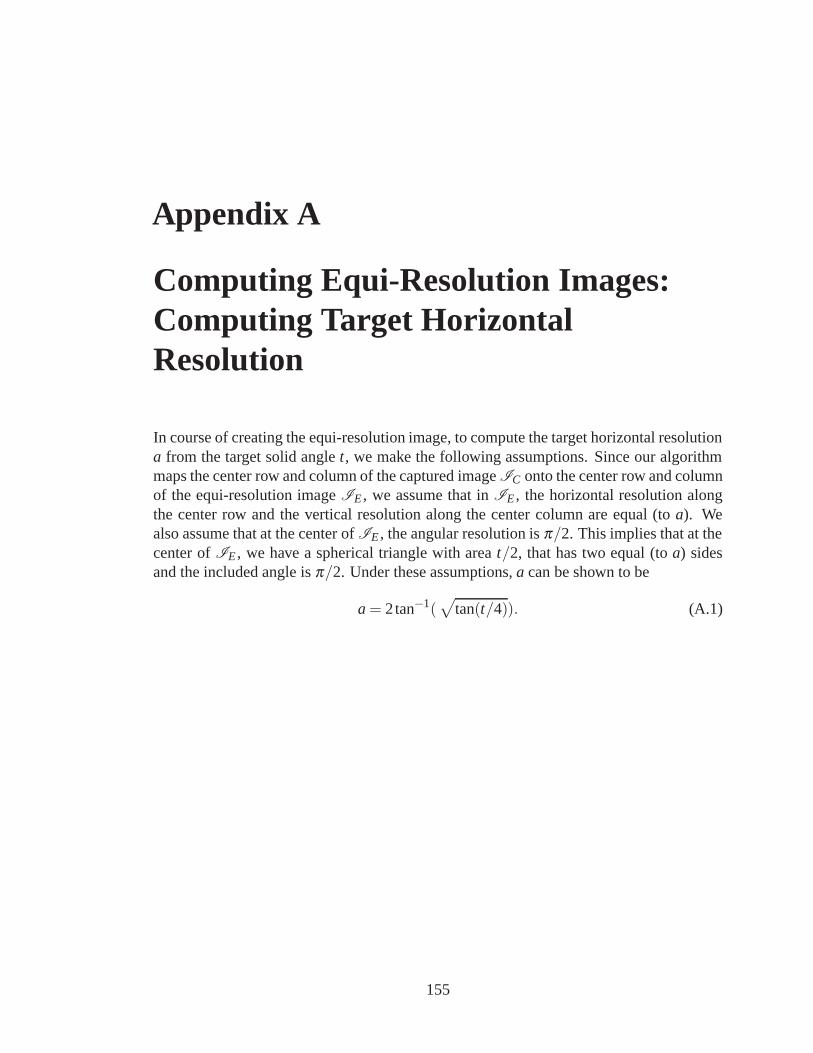
Appendix A

Computing Equi-Resolution Images:Computing Target HorizontalResolution

In course of creating the equi-resolution image, to compute the target horizontal resolutiona from the target solid angle t, we make the following assumptions. Since our algorithmmaps the center row and column of the captured image IC onto the center row and columnof the equi-resolution image IE , we assume that in IE , the horizontal resolution alongthe center row and the vertical resolution along the center column are equal (to a). Wealso assume that at the center of IE , the angular resolution is π/2. This implies that at thecenter of IE , we have a spherical triangle with area t/2, that has two equal (to a) sidesand the included angle is π/2. Under these assumptions, a can be shown to be

a = 2tan−1(√

tan(t/4)). (A.1)

155