Flexibility Based Approach for Damage Characterization: Benchmark Application

hase 1

Dow

nloa

ded

from

asc

elib

rary

.org

by

Dre

xel U

nive

rsity

on

03/1

1/13

. Cop

yrig

ht A

SCE

. For

per

sona

l use

onl

y; a

ll ri

ghts

res

erve

d.

Flexibility Based Approach for Damage Characterization:Benchmark Application

Dionisio Bernal1 and Burcu Gunes2

Abstract: A flexibility based damage characterization technique is described and its performance is examined in the context of Pof the benchmark study developed by the IASC-ASCE SHM Task Group. Noteworthy features of the analytical development are:~1! themethodology used to extract a matrix that is proportional to the flexibility when the excitation is stochastic;~2! the technique used tointerrogate the changes in flexibility~or flexibility proportional matrices! with regards to the location of the damage; and~3! the methodused to quantify the damage without the use of a model. The strategy proved successful in all the cases considered.

DOI: 10.1061/~ASCE!0733-9399~2004!130:1~61!

CE Database subject headings: Damage assessment; Bench marks; Flexibility; Vibration.

aroonresvath

egehetio

roy

nyav

so

atedubdysti

a

1 ofde-red

ivesy

tysethe-hin

p-es:m-

IIxlts

d innd

red

-

ng15

,

uns.witte

o

9/

Introduction

Identification of damage from the analysis of vibration signals hreceived significant attention in the civil, mechanical and aespace fields. The problem most commonly considered is thewhere data are recorded at two different times and it is of inteto determine if the structure suffered damage in the time interbetween the observations. The behavior of the system duringdata collection is typically assumed linear and the damage~whichmay result from an extreme event occurring inside the time sment! is characterized as changes in the parameters of a linmodel. While a solution can in principle be obtained by using tdata to update a model and inspecting the differences, in practhe problem proves to be a difficult one due to a combinationlimited accuracy in the measurements, inevitable modeling erand the need to consider a free parameter space that is usualllarge to attain a well conditioned formulation.

Many techniques that try to circumvent or minimize the madifficulties that arise in the damage characterization problem hbeen proposed~Doebling et al. 1996!. Notwithstanding the sig-nificant volume of work, however, there is a sense that progresthe transfer from research to practical application in the fieldSHM for civil engineering applications has not been entirely sisfactory. In an attempt to clarify the causes for this perceivsituation the dynamics committee of ASCE formed a Task groon Structural Health Monitoring in 1999. The strategy selectedthe ASCE task group was to focus the initial efforts on the stuof a benchmark problem so various identification and diagnotechniques could be tested and compared in a meaningful w

1Associate Professor, Dept. of Civil and Environmental Engineeri427 Snell Engineering Center, Northeastern Univ., Boston, MA 021~corresponding author!. E-mail: [email protected]

2Assistant Professor, Dept. of Civil Engineering, Atilim Univ. H-16Incek, Golbasi 06836. E-mail: [email protected]

Note. Associate Editor: Roger G. Ghanem. Discussion open until J1, 2004. Separate discussions must be submitted for individual paperextend the closing date by one month, a written request must be filedthe ASCE Managing Editor. The manuscript for this paper was submifor review and possible publication on December 27, 2001; approvedJanuary 21, 2003. This paper is part of theJournal of Engineering Me-chanics, Vol. 130, No. 1, January 1, 2004. ©ASCE, ISSN 0733-9392004/1-61–70/$18.00.

JOU

J. Eng. Mech. 20

s-etle

-ar

cefr,too

e

inf-

py

cy.

This paper discusses the strategy used by the writers in Phasethe benchmark study and discusses the results obtained. Thetails of the benchmark structure, the damage scenarios consideand a more elaborate discussion on the background and objectof the IASC-ASCE SHM task group can be found in the paper bJohnson et al. that appears also in this special issue.

This paper contains sections on the extraction of flexibilimatrices, on mapping changes in flexibility to elements whostiffness properties have changed, and on the quantification ofdamaged. The overall strategy is illustrated numerically in ‘‘Numerical Illustration’’ by presenting the analysis of Case 5 witDamage Pattern iv. This case involves asymmetric damageboth directions and is well suited to show the details of the aproach in a general situation. The paper contains two AppendicAppendix I summarizes results obtained for the asymmetric daaged patterns using a model update formulation and Appendixdevelops an expression for the flexibility in terms of the complemodes of the damped system. A complete list of numerical resucan be found in Gunes and Bernal~2001!.

Phase 1 of Benchmark Study

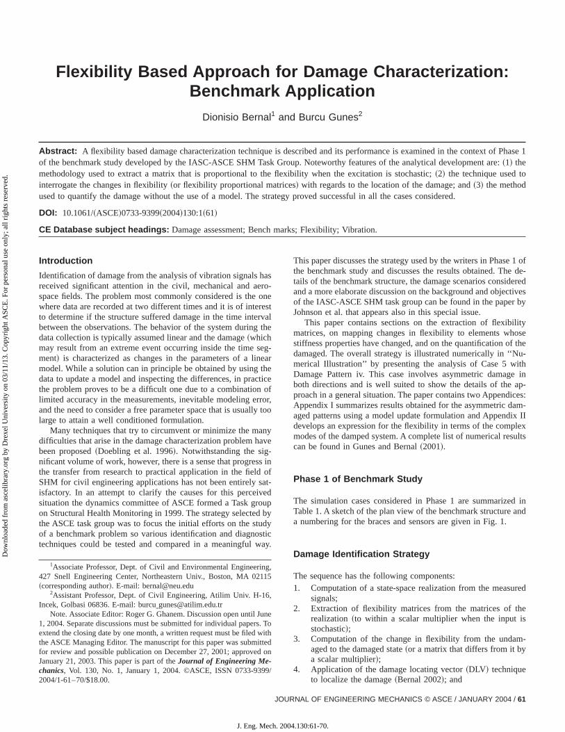
The simulation cases considered in Phase 1 are summarizeTable 1. A sketch of the plan view of the benchmark structure aa numbering for the braces and sensors are given in Fig. 1.

Damage Identification Strategy

The sequence has the following components:1. Computation of a state-space realization from the measu

signals;2. Extraction of flexibility matrices from the matrices of the

realization~to within a scalar multiplier when the input isstochastic!;

3. Computation of the change in flexibility from the undamaged to the damaged state~or a matrix that differs from it bya scalar multiplier!;

4. Application of the damage locating vector~DLV ! techniqueto localize the damage~Bernal 2002!; and

,

eTothdn

RNAL OF ENGINEERING MECHANICS © ASCE / JANUARY 2004 / 61

04.130:61-70.

Dow

nloa

ded

from

asc

elib

rary

.org

by

Dre

xel U

nive

rsity

on

03/1

1/13

. Cop

yrig

ht A

SCE

. For

per

sona

l use

onl

y; a

ll ri

ghts

res

erve

d.

Table 1. Simulation Cases for Phase 1

Parameters Case 1 Case 2 Case 3 Case 4 Case 5

Data generation model Shear building~12 DOF!

Floors rigid in-plane~120 DOF!

Shear building~12 DOF!



Mass distribution Symmetric Symmetric Symmetric Asymmetric AsymmetricExcitation Ambient Ambient Shaker on roof Shaker on roof Shaker on roofID model 12 DOF shear

building12 DOF shear




buildingID data Known input Known input Unknown input Unknown input Unknown input

Unknown input Unknown inputDamage pattern a,b a,b a,b a,b,c,d a,b,c,daAll braces in first story~b1–b8! fail.bAll braces in first and third stories fail~b1–b8, b17–b24!.cBrace b3 fails.dBraces b3 and b18 fail.

urtghfo-escau-s;ph

im

riousthe

u-es.

ion

allyous

n

ts

-

n

5. Quantification of the damage.When sensors are available only on the second and the fofloors and the input is unknown the localization attained throuSteps 2–4 could not be carried out because the available inmation is insufficient to extract the required flexibility proportional matrices. A model update approach was used to addrthese cases, the details of which are described in ‘‘NumeriIllustration’’ under the subheading ‘‘General Model Update Soltion.’’ The following sections elaborate on the previous stepaspects that are well established are presented briefly and emsis is placed on the contributions of this paper.

System Realization

For the deterministic case the state-space model in discrete tcan be expressed as

xk115Axk1Buk (1a)

yk5Cxk1Duk (1b)

and when the input is stochastic as

xk115Axk1wk (2a)

yk5Cxk1vk (2b)

Fig. 1. Floor plan~numbers shown are for level 1 and continue isame pattern in subsequent floors!

62 / JOURNAL OF ENGINEERING MECHANICS © ASCE / JANUARY 2004

J. Eng. Mech. 200

h

r-

sl

a-

e

In the previous expressionsA, B, C, andD5matrices of the real-ization; uk5excitation vector;xk and yk5state and output vec-tors; and in the stochastic input case,wk andvk5~assumed to be!independent stationary white noise sequences. There are vatechniques for extracting the matrices of a realization frommeasurements. In this paper the@ERA-OKID# algorithm is usedwhen the input is known~Juang and Pappa 1985! and a subspacetechnique known as Sub-Id~Van Overschee and Moor 1996!when the input is stochastic. Detailed descriptions of the formlations for both techniques can be found in the listed referenc

Continuous Time ExpressionsIn continuous time the finite difference formulation in Eq.~1!becomes the matrix differential equation given in Eqs.~3!

x5Acx1Bcu (3a)

y5Cx1Du (3b)

As the notation indicates, the matricesC andD are identical in thediscrete time and the continuous time formulations; the relatbetweenAc and Bc and their discrete counterparts are~see forexample Juang 1994!

Ac5log~A!

Dt(4)

and

Bc5~A2I !21AcB (5)

whereDt5sampling time step.

Computation of Flexibility Matrices from RealizationResults

Deterministic InputEven though in the benchmark exercise the structure is classicdamped we consider here the general case of arbitrary viscdamping. In Appendix II it is shown that the flexibility matrix cabe expressed as

F52CDgCT (6)

where Dg5diagonal matrix containing normalization constanand the matrixC contains arbitrarily scaled mode shapes~includ-ing the conjugate pairs!. In the deterministic identification prob

4.130:61-70.

heonas

t tha-

ut is

trixorre

gnat.colow

isa-

s;

sedifoa

theifiedpo

tythis

ates

e

-

esnr-

toem

Therbi-

rof

n

ei-f ar-

ilythe

ly

l.r-notsed

rix.ute

Dow

nloa

ded

from

asc

elib

rary

.org

by

Dre

xel U

nive

rsity

on

03/1

1/13

. Cop

yrig

ht A

SCE

. For

per

sona

l use

onl

y; a

ll ri

ghts

res

erve

d.

lem the mode shapes can be computed at all coordinates wthere is either an output or an input, provided there is, at least,collocated input–output pair. The need for collocation of at leone coordinate will be apparent from the derivation.

The first step in deriving the expressions needed to extracflexibility from the realization is to obtain an input–output reltionship. Taking a Fourier transform of Eqs.~3! and combiningthe expressions one gets

y~v!5@C@ I i v2Ac#21Bc1D#u~v! (7)

or, in terms of the displacement vector,yD

yD~v!51

~ iv!p@C@ I i v2Ac#

21Bc1D#u~v! (8)

wherep50, 1, or 2 depending on whether the measured outpdisplacement, velocity, or acceleration. Evaluating Eq.~8! at v50one obtains an expression for the rows of the flexibility maassociated with the output coordinates and the columns csponding to the inputs, namely

Fm,r52CAc2~p11!Bc (9)

where the fact thatD[0 for velocity and displacement sensinhas been accounted for. Needless to say, when all the coordiare collocated there is no need for further processing since Eq~9!provides the flexibility. In the usual case where there are nonlocated coordinates, however, the process continues as follthe modal amplitudes at the output sensors are given by

Cm5Cw (10)

whereC5state to output mapping matrix andw is such that

Ac5wLew21 (11)

whereLe is diagonal; substituting Eqs.~10! and~11! into Eq. ~9!gives

Fm,r52CmLe2~p11!wBc (12)

where, for notational convenience, we defined

w5w21 (13)

Assume now thatCm is partitioned as

Cm5 HCmm

CmrJ (14)

where Cmm refers to the coordinates where only the outputmeasured andCmr to the collocated coordinates. The normaliztion constants can be obtained by equating them, r partition ofEq. ~6! with Eq. ~12!, from the relationship one gets

dg, j5Le, j2~p11!w j

TBcc@diag~Cmr! j #21 (15)

wheredg, j5jth entry of the diagonal matrixDg ; w jT5jth row of

w; Bcc5columns ofBc corresponding to collocated coordinateand Le, j5jth complex eigenvalue of the system matrix@see Eq.~11!#. Note that the result in Eq.~15! is a row vector containingone estimate ofdg, j for each collocated coordinate. While theestimates are identical for perfect data, in practice the valuesfer because the eigensolution is not exact. A reasonable apprto resolve the redundancy is to takedg as the value for which theentry in (Cmr) j has the largest absolute value. The rationale inprevious suggestion is based on the fact that for any identmode the ratio between amplitudes is most accurate for com

JOU

J. Eng. Mech. 200

reet

e

-

es

-s:

-ch

-

nents that are significant. At this point anm3m flexibility can becomputed by substituting the results from Eqs.~10! and~15! intoEq. ~6!. If there are noncollocated inputs, however, the flexibilifor these coordinates can be also computed; to illustrate howcan be done assume the mode shape vector is expanded to

C5F Cm

CnciG (16)

where the subscript nci is used to note that these are coordinthat correspond to noncollocated input locations. TakingBc,nci asthe columns ofBc that correspond to noncollocated inputs oncan easily confirm, by inspecting Eq.~12!, that

Cnc,jT 5

Le, j2~p11!w j

TBc,nci

dg, j(17)

The complete flexibility follows from Eq.~6! with the modeshapes expanded according to Eq.~16!.

Stochastic InputIf only output signals are available the flexibility cannot be computed using the expressions previously derived because theB ma-trix cannot be extracted from the data. When some conditions~tobe outlined! are met, however, it is possible to extract matricthat differ from the flexibility by a scalar multiplier and these cabe used to replace the flexibility without any loss of useful infomation.

Two introductory comments appear appropriate. The first isnote that we carry out the discussion not for the true syst~which is invariably infinitely dimensional!, but for a finite di-mensional model that is accurate in a certain frequency band.second one is that while the procedures can be derived for atrary damping, the associated complications did not appear~to thewriters! to be justified by the final product and we opted, fosimplicity and clarity, to restrict the presentation to the casereal modes.

We begin by recalling that the flexibility matrix can be writteas

F5(i 51

N

f if iTl i

21 (18)

where,f i andl i5ith mass normalized mode and undampedgenvalue. Expressing the mass normalized modes in terms obitrarily normalized ones one has

f i5f idi (19)

where di5mass normalization constants. Since the arbitrarscaled modes and the eigenvalues are readily obtained fromidentification the problem of assembling the flexibility is simpone of devising a way to compute the constants in Eq.~19!. Arecently proposed approach to extract the constantsdi is based onretesting the structure with a perturbed mass matrix~by adding aknown mass at a certain location! and exploiting the eigenvaluesensitivity equations~Brinker and Andersen 2002; Parloo et a2002!. In the benchmark study the possibility for performing peturbed mass simulations was not available so this option wasexplored. The two techniques presented here are ultimately baon orthogonality of the modes with respect to the mass matBoth techniques, as shown in the following paragraphs, compthe constantsdi to within a missing multiplier common to all themodes.


4.130:61-70.

ialcoroaa

s a

thfat

et-

n

tis

he

satrsn

ble

iesan

a

so

ingch,thisre-tive,ell

d in

pantoad to

in-ortheot belitye

ofns

en-he

ruc-

e-

al-

ex

Dow

nloa

ded

from

asc

elib

rary

.org

by

Dre

xel U

nive

rsity

on

03/1

1/13

. Cop

yrig

ht A

SCE

. For

per

sona

l use

onl

y; a

ll ri

ghts

res

erve

d.

Methodology No. 1. This option can be used when all the inertcoordinates are measured. The idea is simply to use thestraints provided by mass orthogonality to extract a matrix pportional to the mass and then use this matrix directly to normize the modes in the usual way. Specifically, assume the mmatrix can be parameterized as shown in

M5(i 51

p

a iEi (20)

where p5number of free parameters;Ei5elementary matricesthat depend on the structure of the mass matrix; anda i5unknownparameters. Orthogonality of the modes with respect to maslows one to write

(i 51

p

(j 51

q

(k5 j 11

q

a if jTEifk50 (21)

where q5number of identified modes. Eq.~21! can be reorga-nized and expressed as

Sa50 (22)

Eq. ~22! can, of course, be formulated for the reference anddamaged state and, under the assumption that the mass osystem has not changed as a result of the damage, the informfrom both states can be combined and one gets

FSu

SdG$a%5Sa50 (23)

where the subscriptsu and d indicate the undamaged and thpotentially damaged conditions. An examination shows thaSPRY3p with Y5qt(qt21)/2; whereqt5sum of the modes identified in both states. Inspecting the number of rows and columone concludes that a necessary condition forS to be rank deficientby no more than one is that the number of identified modes sa

qt~qt21!>2~p11! (24)

Methodology No. 2. When the sensor set is not complete tprevious approach cannot be used~at least without resorting tosome expansion of the mode to the unmeasured coordinate!. Amethod based on the expression for the inverse of the mass moffers, however, a possible alternative. The partition of the inveof the mass associated with the measured coordinates is give

M 215(i 51

N

f if iTdi

2 (25)

A first possibility is to use any information that may be availaregardingM 21 to set up equations to computedi , for example, itmay be reasonable to assume thatM 21 is diagonal and in thiscase one can use the off diagonal zeros as constraints~Bernal andGunes 2002!. A second modality is to subtract the modal serexpressions forM 21 for the reference and the damaged stateto use the zeros that are created by the operation~since we as-sume that the mass does not change as a result of the dam!.Note, however, that since all the modalities that use Eq.~25! arebased on equating a modal series to a physical quantity, thetions are exact only when all the modes are available.


J. Eng. Mech. 20

n--l-ss

l-

etheion

s

fy

rixeby

d

ge

lu-

Damage Localization

A general approach to interrogate changes in flexibility regardspatial localization of damage, designated as the DLV approahas been recently developed and was used by the authors inphase of the benchmark study. The discussion that follows psents the basic features of the technique from a user’s perspeca more detailed discussion of the theoretical background as was discussion on robustness and other issues may be founBernal ~2002!.

Damage Locating Vector TechniqueThe basic idea in the DLV approach is that the vectors that sthe null space of the change in flexibility from the undamagedthe damaged states, when treated as loads on the system, lestress fields that are zero over the damaged elements.

Depending on the number and location of the sensors thetersection of the null stress regions identified by the DLVs maymay not contain elements that are not damaged in addition todamaged ones. Elements that are undamaged but which canndiscriminated from the damaged ones by changes in flexibi~for a given set of sensors! are referred to as inseparable. Thsteps of the DLV localization can be summarized as follows:1. Compute the change in flexibility as

DF5FD2FU (26)

2. Obtain a singular value decomposition ofDF, namely

DF5UFS1 0

0 s2GVT (27)

wheres25‘‘small’’ singular values. For ideal conditions thes2’s5zeros and the DLV vectors are simply the columnsV associated with the null space. For the noisy conditiothat prevail in practice, however, the values ins2 never equalzero and a cutoff has to be established to select the dimsion of the effective null space. The rationale behind tprocedure to select which vectors inV that can be treated asDLVs is described in Bernal~2002!.

3. Compute the stresses in an undamaged model of the stture using the vectors inV as loads.

4. For any vectorVj , reduce the internal stresses in every elment to a single characterizing stress,s i ~strain energy perunit characterizing dimension should be proportional tos i

2).Definecj ~where the subscript identifies the column ofV) as

cj5minS 1

siD (28)

5. Compute the svn index as

svnj5Asjcj2

sqcq2

(29)

wheresi5ith singular value and

sqcq25max~sjcj

2! for j51:m (30)

6. The vectorVj can be treated as a DLV if

svnj<0.20 (31)

Once the set of DLV vectors have been identified the locization proper is carried out as follows:

7. Compute, for each DLV vector, the normalized stress ind

4

04.130:61-70.

sll.

ifiessveup

thsiff-arsis

l

-i-c-

esm

ofrr

theuth

d

tedfie

a-d asandcan

e totby

red

te

vi-eri-ablef the

e 5

sed.the

gure

t

allose-real.the

tifieduracy

Dow

nloa

ded

from

asc

elib

rary

.org

by

Dre

xel U

nive

rsity

on

03/1

1/13

. Cop

yrig

ht A

SCE

. For

per

sona

l use

onl

y; a

ll ri

ghts

res

erve

d.

vector ~one entry per element in the structure! as

nsij5cjs (32)

8. Compute the vector of weighted stress indices~WSI! as

WSI5

(i51

ndlvnsiisvni

ndlv(33)

where

svni5max~svni ,0.015! (34)

and ndlv5number of DLV vectors.9. The potentially damaged elements are those having WSI,1.It should be stressed that the steps and limits shown previouare unrelated to the benchmark exercise and apply in genera

Quantification

When there are sensors at all floors the damaged is quantfrom the identification results as changes in interstory stiffneWhen sensors are available only at the second and fourth lethe damage is quantified at the element level using a modeldate strategy based on the eigenvalue equation.

Full Sensor Set„12 Degree of Freedom Measured…We define the interstory stiffness as the shear associated wiunit drift in the level of interest when the drift in all other leveland all the twists are zero. The coordinate of the center of stness is simply the intersection of the lines of actions of the shegenerated by unit drifts in each of the two orthogonal directionOne can confirm that the interstory stiffness defined this waygiven by

kj5d jTF2* d j (35)

whered j5displacement vector that imposes a unit drift at levej~in the direction of analysis! and the symbol* is used to indicatethe pseudoinverse operation~to cover the case where the flexibility is rank deficient!. It can be easily confirmed that the coordnate of the center of stiffness in the direction normal to the diretion where the drift is imposed is given by

ej5rTF2* d j

d jTF2* d j

(36)

wherer5vector that contains ordered values listing the distancfrom the various forces to the origin of the coordinate syste~with 1s when the entries are torques!. Note that the previousdefinition of interstory stiffness decouples the quantificationthe damage in the two orthogonal directions and does not cathe assumption that the system behaves as a shear beam.

General Model Update SolutionThe previous quantification approach cannot be applied incase where there are sensors only at the second and the fofloors because the measurements are insufficient to extractinterstory stiffness values. The model update approach useconsider these cases is outlined next.

When analytical and experimental quantities are substituinto the eigenvalue problem the equation is not generally satisand one can define an error vector for modej as

« j5K~uk!f j2M ~um!f jl j (37)

JOU

J. Eng. Mech. 200

y

d.ls-

a

s.

y

rthe

to

d

whereuk andum5free parameters in the stiffness and mass mtrices, respectively. Assume that the mode shape is partitione@f1 f2#T, where the subscripts 1 and 2 refer to measuredunmeasured coordinates, with this notation the error vectoralso be written in partitioned form as

$« j%5 H «1,j

«2,jJ (38)

where one can easily confirm that

«1,j5~k112m11l j !f1,j2~k122m12l j !f2,j (39)

and

«2,j5~k212m21l j !f1,j2~k222m22l j !f2,j (40)

In the previous equations we have eliminated explicit referencuk andum to simplify the notation. From Eq.~40! one can see thathe second partition of the error vector is made identically zerotaking

f2,j5~k222m22l j !21~k212m21l j !f1,j (41)

which is simply an expansion of the mode to the unmeasucoordinates. Substituting Eq.~41! into Eq. ~40! one gets

« j5 b~k112m11l j !2~k122m12l j !~k222m22l j !21

3~k212m21l j !cf1,j (42)

where the subscript 1 has been eliminated from«. In Eq. ~42! l j

and f1,j are available from the identification; the model updaconsists of the selection of the free parametersuk and um tominimize

J5(j 51

q

« jT« jv j (43)

wherev j5weighting constants. A desirable feature of the preous formulation is the fact that there is no need to pair expmental and analytical modes; on the other hand, an undesirfeature is the fact that the error terms depend on the scaling omeasured modes. In the numerical analysis we normalizedf1,j tounit length.

Numerical Illustration

We illustrate the previous techniques on the analysis of Caswith damaged pattern iv~see Table 1!. Consider first the situationwhere there are sensors in all the levels.

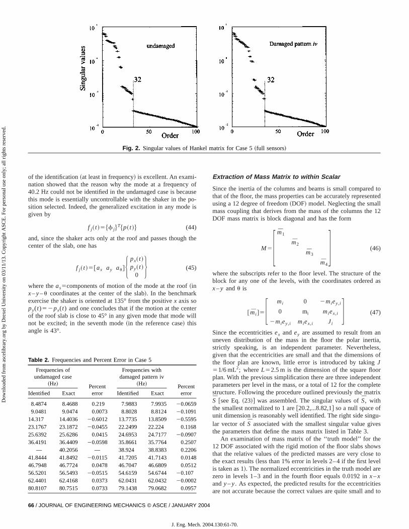
Realization

The output was sampled at 0.004 and 80 s of signal were uThe singular values of the Hankel matrix for the reference anddamaged case are shown in Fig. 2. From the results in the fithe order of the system was initially selected as 32~both in thereference and the damaged condition! but the modes that did nosatisfy the criteria@damping,5%, frequency,100 Hz~0.8 of Ny-quist! and mpcw.90%# were assumed to be computationmodes and discarded. The mpcw coefficient measures the cness by which the phases of the modal entries differ by zero opand it equals 100% when the mode can be normalized to rThere were 11 modes that satisfied the previous criteria inundamaged case and 12 in the damaged condition. The idenfrequencies are depicted in Table 2; as can be seen, the acc


4.130:61-70.

Dow

nloa

ded

from

asc

elib

rary

.org

by

Dre

xel U

nive

rsity

on

03/1

1/13

. Cop

yrig

ht A

SCE

. For

per

sona

l use

onl

y; a

ll ri

ghts

res

erve

d.

Fig. 2. Singular values of Hankel matrix for Case 5~full sensors!

yu

poe

h

tei

d tonted

12

theas

nia,ess,s of

rentleterix

u-es

wse tolre

iesnd to

76812

57

of the identification~at least in frequency! is excellent. An exami-nation showed that the reason why the mode at a frequenc40.2 Hz could not be identified in the undamaged case is becathis mode is essentially uncontrollable with the shaker in thesition selected. Indeed, the generalized excitation in any modgiven by

f j~ t !5$f j%T$p~ t !% (44)

and, since the shaker acts only at the roof and passes thougcenter of the slab, one has

f j~ t !5@ax ay au#H px~ t !py~ t !

0J (45)

where theas5components of motion of the mode at the roof~inx–y–u coordinates at the center of the slab!. In the benchmarkexercise the shaker is oriented at 135° from the positivex axis sopy(t)52px(t) and one concludes that if the motion at the cenof the roof slab is close to 45° in any given mode that mode wnot be excited; in the seventh mode~in the reference case! thisangle is 43°.

Table 2. Frequencies and Percent Error in Case 5

Frequencies ofundamaged case

~Hz! Percenterror

Frequencies withdamaged pattern iv

~Hz! PercenterrorIdentified Exact Identified Exact

8.4874 8.4688 0.219 7.9883 7.9935 20.06599.0481 9.0474 0.0073 8.8028 8.812420.1091

14.317 14.4036 20.6012 13.7735 13.8509 20.559523.1767 23.1872 20.0455 22.2499 22.224 0.116825.6392 25.6286 0.0415 24.6953 24.717720.090736.4191 36.4409 20.0598 35.8661 35.7764 0.250

— 40.2056 — 38.924 38.8383 0.22041.8444 41.8492 20.0115 41.7205 41.7143 0.01446.7948 46.7724 0.0478 46.7047 46.6809 0.0556.5201 56.5493 20.0515 54.6159 54.6744 20.10762.4401 62.4168 0.0373 62.0431 62.043220.000280.8107 80.7515 0.0733 79.1438 79.0682 0.09


J. Eng. Mech. 2

ofse-is

the

rll

Extraction of Mass Matrix to within Scalar

Since the inertia of the columns and beams is small comparethat of the floor, the mass properties can be accurately represeusing a 12 degree of freedom~DOF! model. Neglecting the smallmass coupling that derives from the mass of the columns theDOF mass matrix is block diagonal and has the form

M5F m1

m2

m3

m4

G (46)

where the subscripts refer to the floor level. The structure ofblock for any one of the levels, with the coordinates orderedx–y andu is

@mi #5F mi 0 2miey,i

0 mi miex,i

2miey,i miex,i Ji

G (47)

Since the eccentricitiesex and ey are assumed to result from auneven distribution of the mass in the floor the polar inertstrictly speaking, is an independent parameter. Neverthelgiven that the eccentricities are small and that the dimensionthe floor plan are known, little error is introduced by takingJ51/6 mL2; whereL52.5 m is the dimension of the square flooplan. With the previous simplification there are three independparameters per level in the mass, or a total of 12 for the compstructure. Following the procedure outlined previously the matS @see Eq.~23!# was assembled. The singular values ofS, withthe smallest normalized to 1 [email protected],...8.82,1# so a null space ofunit dimension is reasonably well identified. The right side singlar vector ofS associated with the smallest singular value givthe parameters that define the mass matrix listed in Table 3.

An examination of mass matrix of the ‘‘truth model’’ for the12 DOF associated with the rigid motion of the floor slabs shothat the relative values of the predicted masses are very closthe exact results~less than 1% error in levels 2–4 if the first leveis taken as 1!. The normalized eccentricities in the truth model azero in levels 1–3 and in the fourth floor equals 0.0192 inx–xandy–y. As expected, the predicted results for the eccentricitare not accurate because the correct values are quite small a

4

004.130:61-70.

me

aa

en

e

e

e

foaa

g

-thatee

mt

o

dt thetheifi-error

t theach-f the

liedings-

thee adesultsthe

odel

d innotrnal

e, asagellytrat-

onlyetric

ofnalhe

ti-

Dow

nloa

ded

from

asc

elib

rary

.org

by

Dre

xel U

nive

rsity

on

03/1

1/13

. Cop

yrig

ht A

SCE

. For

per

sona

l use

onl

y; a

ll ri

ghts

res

erve

d.

extract them correctly it is necessary to have accurate modal aplitudes in the nondominant directions for each one of the modfor example, in a mode that is essentially translation inx–x, oneneeds accurate rotations. The identified eccentricities areequate, however, in the sense that they indicate that the mmatrix is essentially diagonal.

Extraction of Flexibility Matrices (to within Scalar)

With the mass matrix identified to within a scalar multiplier thmode shapes for the damaged and the undamaged states canormalized without difficulty. The flexibility matrices to withinthe same missing scalar can then be computed and the changflexibility obtained by subtracting one matrix from the other.

Damage Localization

Albeit only for the purpose of a static analysis the DLV techniqurequire the introduction of a model~although the model may belimited to geometrical information if the quantity used to locatthe damage is statically determinate!. In the case considered herewe attempted to locate the damage at the element level and,lowing the guidelines of Phase 1 this is done by using a shebuilding. The computations show that there are four vectors thsatisfy the DLV criterion~svn<0.20!, the results for the WSI aresummarized in Table 4.

As can be seen, the DLV localization correctly locates dama~WSI,1! on the right sidey–y direction frame on Level 1 and onLevel 3 of thex–x frame located on the lower side.

Quantification

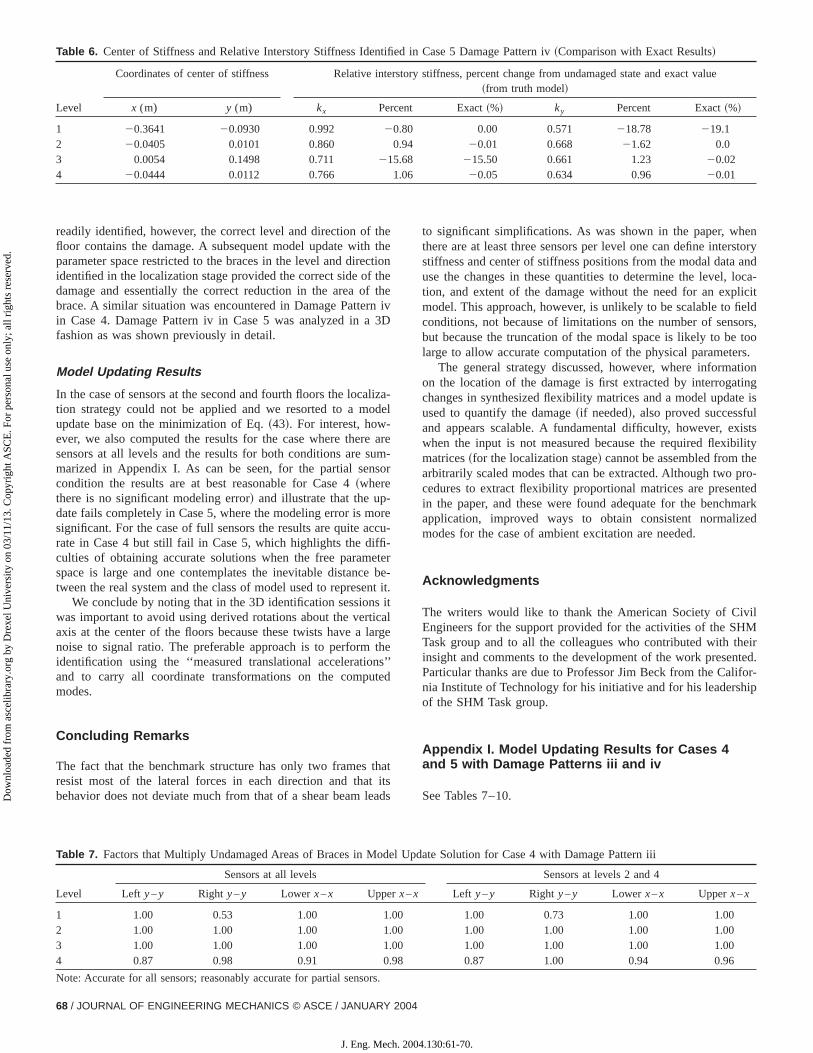
The interstory stiffness computed from Eq.~35! and the eccen-tricities from Eq.~36! are listed in Tables 5 and 6 for the undamaged and the damaged condition, respectively. We recall thatinterstory stiffness values are available only to within a scalmultiplier when the input is not measured so the results presenare for an arbitrary normalization. Table 6 shows, in addition, thidentified percent change in interstory stiffness from the undaaged to the damaged condition and the exact values compufrom the truth model.

As can be seen, only Level 3 inx–x and 1 iny–y ~the correctlocations of the damage! display significant changes in the inter-story stiffness and the shift in the coordinate of the center

Table 3. Results for Parameters that Define Mass Matrix

Level Mass~relative! ey /L ex /L

1 1 0.002 20.0042 0.768 0.007 0.0113 0.768 0.015 0.0114 0.573 0.021 0.040

Table 4. Weighted Stress Index Indices for Case 5 Damage Pattern

Level

Frames iny–y direction Frames inx–x direction

Left side Right side Lower side Upper side

1 1.52 0.59a 6.23 5.502 4.51 2.97 1.87 3.573 3.63 1.65 0.29a 3.674 4.84 3.42 1.19 1.81aLocation of true damage.

JOU

J. Eng. Mech. 20

-s;

d-ss

be

in

l-rt

e

erd

-ed

f

stiffness shows~confirms! that the damage is unsymmetrical anwhich side has suffered the largest loss. Furthermore, note thaidentified loss of interstory stiffness is in good agreement withvalue from the truth model. This is to be expected if the identcation is reasonably accurate because there is no modelingassociated with the formulation used here.

Partial Sensors

We consider the situation when sensors are available only asecond and fourth levels by applying the model update approassociated with Eq.~43!. Since there is no localization information available we take the free parameters as the 16 areas obraces~one area covers two physical braces!. The mass matrix istaken as diagonal with entries equal to the true values multipby numbers selected randomly from a uniform distribution havlimits of 0.9 and 1.1~the eccentricity of the roof mass was asumed unknown and therefore not modeled!. Constraints wereintroduced so that the identified areas could not be larger thanundamaged ones or less than zero. No attempts to providweighting matrix that reflected perceived accuracy on the mowas made so the weights were all taken as unity. The resobtained are summarized in Appendix I and are discussed innext section in connection with the other cases where the mupdate approach was used.

Other Results

In this section we comment on the numerical results obtainethe complete exercise; the full set of numerical results ispresented for brevity but can be found in Gunes and Be~2001!.

Damage Patterns i and ii

These damaged patterns are symmetrical and very extensivexpected, no difficulties were encountered in locating the damwith the DLV approach and the quantification proved virtuaexact in the case of sensors at all levels. The model update segy used in the case of partial sensors was also successful.

Damage Patterns iii and iv (Sensors at All Levels)

These damage patterns are asymmetrical and are consideredin Cases 4 and 5 where the structure is also slightly asymmdue to a shift in the mass at the fourth level. The localizationthe damage in pattern iii from the results of a three-dimensio~3D! identification proved difficult because the accuracy of ttorsional mode shapes~specially in the undamaged state! wasinadequate. Application of the DLV approach inx–x andy–y is

iv

Table 5. Center of Stiffness and Relative Interstory Stiffness Idenfied in Undamaged Condition~Case 5!

Level

Coordinates of center of stiffness~see axes in Fig. 1!

Relative interstorystiffness

x (m) y (m) kx ky

1 0.0262 20.0232 1 0.7032 20.0714 20.1140 0.852 0.6793 0.0658 20.0423 0.843 0.6534 20.0490 20.0780 0.758 0.628


04.130:61-70.

Dow

nloa

ded

from

asc

elib

rary

.org

by

Dre

xel U

nive

rsity

on

03/1

1/13

. Cop

yrig

ht A

SCE

. For

per

sona

l use

onl

y; a

ll ri

ghts

res

erve

d.

Table 6. Center of Stiffness and Relative Interstory Stiffness Identified in Case 5 Damage Pattern iv~Comparison with Exact Results!

Coordinates of center of stiffness Relative interstory stiffness, percent change from undamaged state and exact value~from truth model!

Level x (m) y (m) kx Percent Exact~%! ky Percent Exact~%!

1 20.3641 20.0930 0.992 20.80 0.00 0.571 218.78 219.12 20.0405 0.0101 0.860 0.94 20.01 0.668 21.62 0.03 0.0054 0.1498 0.711 215.68 215.50 0.661 1.23 20.024 20.0444 0.0112 0.766 1.06 20.05 0.634 0.96 20.01

hethtio

thethiv

3D

lizade

aumsor

orecu-teb

ntit

caargthes’’

ted

haitsad

ntoryndca-

citldrs,

toos.ionng

is

stslity

ro-edarkd

lMir

ed.or-p

readily identified, however, the correct level and direction of tfloor contains the damage. A subsequent model update withparameter space restricted to the braces in the level and direcidentified in the localization stage provided the correct side ofdamage and essentially the correct reduction in the area ofbrace. A similar situation was encountered in Damage Patternin Case 4. Damage Pattern iv in Case 5 was analyzed in afashion as was shown previously in detail.

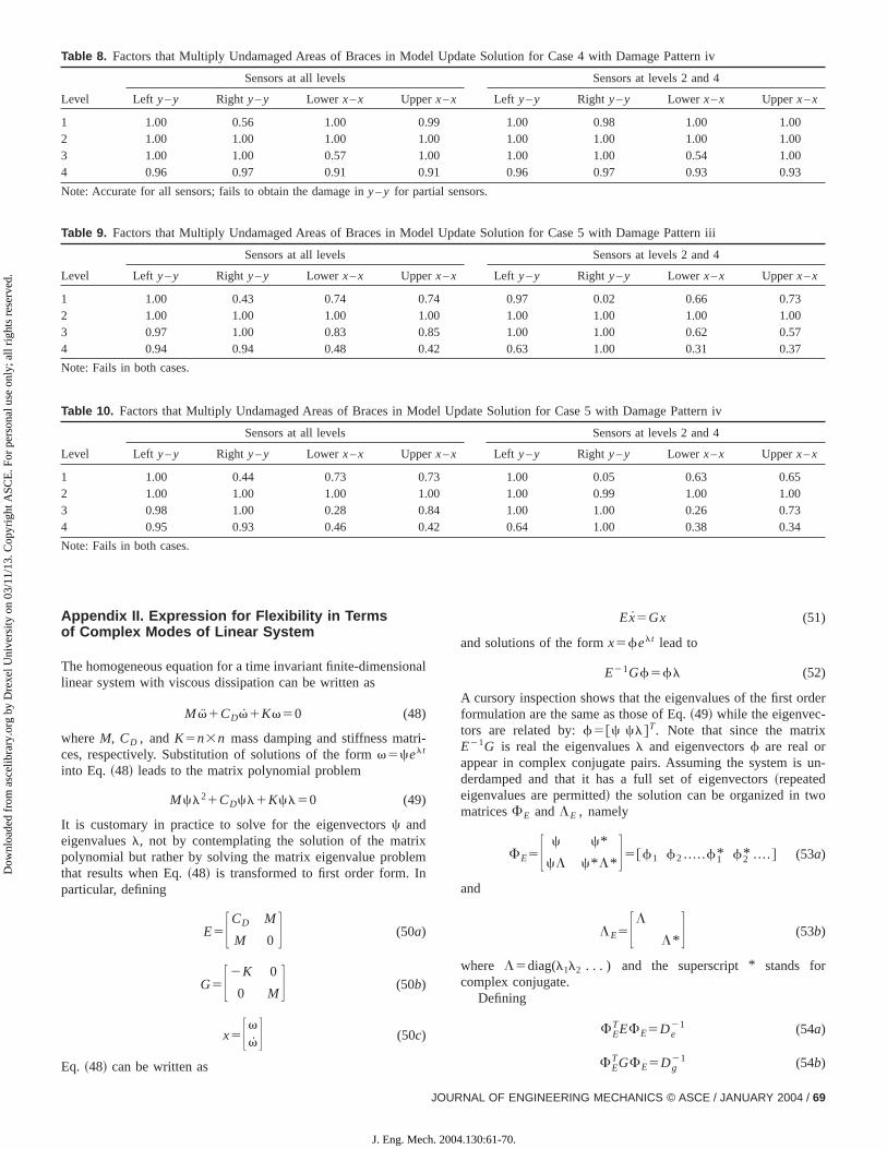
Model Updating Results

In the case of sensors at the second and fourth floors the location strategy could not be applied and we resorted to a moupdate base on the minimization of Eq.~43!. For interest, how-ever, we also computed the results for the case where theresensors at all levels and the results for both conditions are smarized in Appendix I. As can be seen, for the partial sencondition the results are at best reasonable for Case 4~wherethere is no significant modeling error! and illustrate that the up-date fails completely in Case 5, where the modeling error is msignificant. For the case of full sensors the results are quite acrate in Case 4 but still fail in Case 5, which highlights the difficulties of obtaining accurate solutions when the free paramespace is large and one contemplates the inevitable distancetween the real system and the class of model used to represe

We conclude by noting that in the 3D identification sessionswas important to avoid using derived rotations about the vertiaxis at the center of the floors because these twists have a lnoise to signal ratio. The preferable approach is to performidentification using the ‘‘measured translational accelerationand to carry all coordinate transformations on the compumodes.

Concluding Remarks

The fact that the benchmark structure has only two frames tresist most of the lateral forces in each direction and thatbehavior does not deviate much from that of a shear beam le


J. Eng. Mech. 200

en

e

-l

re-

-

re-it.

le

t

s

to significant simplifications. As was shown in the paper, whethere are at least three sensors per level one can define intersstiffness and center of stiffness positions from the modal data ause the changes in these quantities to determine the level, lotion, and extent of the damage without the need for an explimodel. This approach, however, is unlikely to be scalable to fieconditions, not because of limitations on the number of sensobut because the truncation of the modal space is likely to belarge to allow accurate computation of the physical parameter

The general strategy discussed, however, where informaton the location of the damage is first extracted by interrogatichanges in synthesized flexibility matrices and a model updateused to quantify the damage~if needed!, also proved successfuland appears scalable. A fundamental difficulty, however, exiwhen the input is not measured because the required flexibimatrices~for the localization stage! cannot be assembled from thearbitrarily scaled modes that can be extracted. Although two pcedures to extract flexibility proportional matrices are presentin the paper, and these were found adequate for the benchmapplication, improved ways to obtain consistent normalizemodes for the case of ambient excitation are needed.

Acknowledgments

The writers would like to thank the American Society of CiviEngineers for the support provided for the activities of the SHTask group and to all the colleagues who contributed with theinsight and comments to the development of the work presentParticular thanks are due to Professor Jim Beck from the Califnia Institute of Technology for his initiative and for his leadershiof the SHM Task group.

Appendix I. Model Updating Results for Cases 4and 5 with Damage Patterns iii and iv

See Tables 7–10.

Table 7. Factors that Multiply Undamaged Areas of Braces in Model Update Solution for Case 4 with Damage Pattern iii

Level

Sensors at all levels Sensors at levels 2 and 4

Left y–y Right y–y Lower x–x Upperx–x Left y–y Right y–y Lower x–x Upperx–x

1 1.00 0.53 1.00 1.00 1.00 0.73 1.00 1.002 1.00 1.00 1.00 1.00 1.00 1.00 1.00 1.003 1.00 1.00 1.00 1.00 1.00 1.00 1.00 1.004 0.87 0.98 0.91 0.98 0.87 1.00 0.94 0.96

Note: Accurate for all sensors; reasonably accurate for partial sensors.

4.130:61-70.

Dow

nloa

ded

from

asc

elib

rary

.org

by

Dre

xel U

nive

rsity

on

03/1

1/13

. Cop

yrig

ht A

SCE

. For

per

sona

l use

onl

y; a

ll ri

ghts

res

erve

d.

Table 8. Factors that Multiply Undamaged Areas of Braces in Model Update Solution for Case 4 with Damage Pattern iv

Level



1 1.00 0.56 1.00 0.99 1.00 0.98 1.00 1.002 1.00 1.00 1.00 1.00 1.00 1.00 1.00 1.003 1.00 1.00 0.57 1.00 1.00 1.00 0.54 1.004 0.96 0.97 0.91 0.91 0.96 0.97 0.93 0.93

Note: Accurate for all sensors; fails to obtain the damage iny–y for partial sensors.

Table 9. Factors that Multiply Undamaged Areas of Braces in Model Update Solution for Case 5 with Damage Pattern iii

Level



1 1.00 0.43 0.74 0.74 0.97 0.02 0.66 0.732 1.00 1.00 1.00 1.00 1.00 1.00 1.00 1.003 0.97 1.00 0.83 0.85 1.00 1.00 0.62 0.574 0.94 0.94 0.48 0.42 0.63 1.00 0.31 0.37

Note: Fails in both cases.

Table 10. Factors that Multiply Undamaged Areas of Braces in Model Update Solution for Case 5 with Damage Pattern iv

Level



1 1.00 0.44 0.73 0.73 1.00 0.05 0.63 0.652 1.00 1.00 1.00 1.00 1.00 0.99 1.00 1.003 0.98 1.00 0.28 0.84 1.00 1.00 0.26 0.734 0.95 0.93 0.46 0.42 0.64 1.00 0.38 0.34

Note: Fails in both cases.

a

-

m

er

n-

Appendix II. Expression for Flexibility in Termsof Complex Modes of Linear System

The homogeneous equation for a time invariant finite-dimensionlinear system with viscous dissipation can be written as

M v1CDv1Kv50 (48)

whereM, CD , andK5n3n mass damping and stiffness matrices, respectively. Substitution of solutions of the formv5celt

into Eq. ~48! leads to the matrix polynomial problem

Mcl21CDcl1Kcl50 (49)

It is customary in practice to solve for the eigenvectorsc andeigenvaluesl, not by contemplating the solution of the matrixpolynomial but rather by solving the matrix eigenvalue problethat results when Eq.~48! is transformed to first order form. Inparticular, defining

E5FCD M

M 0 G (50a)

G5F2K 0

0 M G (50b)

x5Fvv G (50c)

Eq. ~48! can be written as

JOU

J. Eng. Mech. 20

l

Ex5Gx (51)

and solutions of the formx5felt lead to

E21Gf5fl (52)

A cursory inspection shows that the eigenvalues of the first ordformulation are the same as those of Eq.~49! while the eigenvec-tors are related by:f5@c cl#T. Note that since the matrixE21G is real the eigenvaluesl and eigenvectorsf are real orappear in complex conjugate pairs. Assuming the system is uderdamped and that it has a full set of eigenvectors~repeatedeigenvalues are permitted! the solution can be organized in twomatricesFE andLE , namely

FE5F c c*

cL c* L* G5@f1 f2 .....f1* f2* ....# (53a)

and

LE5FL

L* G (53b)

where L5diag(l1l2 . . . ) and the superscript * stands forcomplex conjugate.

Defining

FETEFE5De

21 (54a)

FETGFE5Dg

21 (54b)


04.130:61-70.

e-a

Dow

nloa

ded

from

asc

elib

rary

.org

by

Dre

xel U

nive

rsity

on

03/1

1/13

. Cop

yrig

ht A

SCE

. For

per

sona

l use

onl

y; a

ll ri

ghts

res

erve

d.

Dg21 andDe

21 are diagonal; from Eqs.~54! one can write

E215FEDeFET (55a)

G215FEDgFET (55b)

Expanding the expressions in Eqs.~55! and equating the appro-priate partitions to the inverses ofE andG ~in terms ofM, C, andK! one gets~among other relations!

K2152CDgCT (56)

References

Bernal, D. ~2002!. ‘‘Load vectors for damage localization.’’J. Eng.Mech.,128~1!, 7–14.

Bernal, D., and Gunes, B.~2002!. ‘‘Damage localization in output-onlysystems: a flexibility based approach.’’Proc., 20th Modal AnalysisConf. (IMAC XX), Los Angeles, 1185–1191.


J. Eng. Mech. 20

Brinker, R., and Andersen, P.~2002!. ‘‘A way of getting scaled modeshapes in output-only modal testing.’’Proc., 21th Modal AnalysisConf. (IMAC XXI), ~CD Rom! Orlando, Fla.

Doebling, S. C., Farrar, C. R., Prime, M. B., and Schevitz, D. W.~1996!.Damage identification and health monitoring of structural and mchanical systems from changes in their vibration characteristics:literature review, Los Alamos, N.M.

Gunes, B., and Bernal, D.~2001!. ‘‘Identification and localization of dam-age: a flexibility-based approach.’’Rep. No. CEE-4-2001, Dept. ofCivil and Environmental Engineering, Northeastern Univ., Boston.

Juang, J.-N.~1994!. Applied system identification, Prentice-Hall, Engle-wood Cliffs, N.J.

Juang, J., and Pappa, R.~1985!. ‘‘An eigensystem realization algorithmfor modal parameter identification and model reduction.’’J. Guid.Control Dyn.,8~5!, 610–627.

Parloo, E., Verboven, P., Cuillame, P., and Overmeire, M. V.~2002!.‘‘Sensitivity-based operational mode shape normalization.’’Mech.Syst. Signal Process.,16~5!, 757–767.

Van Overschee, P., and Moor, B. L. R.~1996!. Subspace identification forlinear systems: Theory, implementation, applications, Kluwer Aca-demic, Boston.

4

04.130:61-70.

Documents

Flexibility Based Approach for Damage Characterization: Benchmark Application