Embed Size (px)
Citation preview

HAL Id: tel-01157143https://tel.archives-ouvertes.fr/tel-01157143
Submitted on 27 May 2015
HAL is a multi-disciplinary open accessarchive for the deposit and dissemination of sci-entific research documents, whether they are pub-lished or not. The documents may come fromteaching and research institutions in France orabroad, or from public or private research centers.
L’archive ouverte pluridisciplinaire HAL, estdestinée au dépôt et à la diffusion de documentsscientifiques de niveau recherche, publiés ou non,émanant des établissements d’enseignement et derecherche français ou étrangers, des laboratoirespublics ou privés.
Flexibility assessment and management in supply chain :a new framework and applications
Yueru Zhong
To cite this version:Yueru Zhong. Flexibility assessment and management in supply chain : a new framework and appli-cations. Other. Ecole Centrale Paris, 2015. English. <NNT : 2015ECAP0012>. <tel-01157143>

ÉCOLE CENTRALE DES ARTS
ET MANUFACTURES « ÉCOLE CENTRALE PARIS »
THÈSE présentée par
Yueru Zhong
pour l’obtention du
GRADE DE DOCTEUR
Spécialité : Génie Industriel Laboratoire d’accueil : Laboratoire Génie Industriel
Evaluation et Gestion de la Flexibilité dans les Chaînes Logistiques : Nouveau Cadre Général et Applications
soutenue le 30 janvier 2013 à l’Ecole Centrale Paris devant le jury composé de :
FREIN Yannick Professeur à l’Institut national
polytechnique de Grenoble Président du jury
ALLAOUI Hamid Professeur à l’Université d’Artois Rapporteur GRABOT Bernard Professeur à l’École nationale
d'ingénieurs de Tarbes Rapporteur
LECŒUCHE Loïc Manager de Louis Vuitton Examinateur CHU Chengbin Professeur à l’École Centrale Paris Directeur de thèse JEMAI Zied Maître de conférences - HDR à l’Ecole
Nationale d'Ingénieurs de Tunis Co-encadrant de thèse
2015ECAP0012


To my dear parents... who have always been so close to mewhenever I needed. It is their unconditional love, support and
encouragement to motivate me to set higher targets.


Acknowledgments
I would like to express my sincere gratitude to many people who have helped me over theyears of my thesis.
My thanks are directed to all the members of Industrial Engineering Laboratory in EcoleCentral Paris, for their warm companion, their kindness and continuous support. Partic-ular thanks to Prof. Jean-Claude Bocquet, the director of lab, and Anne Prévot, CaroleStoll, Corinne Ollivier, Delphine Martin and Sylvie Guillemain. Thanks to them, mywork has taken place in such a good condition with all their earnest assitances.
This thesis is also the result of collaboration with industrial partners at that time in ChairSupply Chain, namely Carrefour, Danone, Louis Vuitton, PSA and Vallourec. I wishto thank them for their hospitality, their confidence and participation, which helped mequite a lot to gather precious knowledge in industrial world. I would like to express mynumerous thanks to Mr Etienne Marie in Evian and Mr Loïc Lecœuch in Louis Vuitton.Thanks for their hospitality and availability without which I could not have collectedsufficient information and data that have enriched this work and made it possible. Thanksalso to Mr Loïc Lecœuch for having accepted to honor me by participating in the defensecommittee.
My sincere thanks go to the other members of my defense committee who accepted toevaluate this thesis, the two reviewers Prof. Hamid Allaoui and Prof. Bernard Grabot,the examiner Prof. Yannick Frein, for having taken the time even in holidays to read andevaluate my work, for their insightful comments and constructive questions and for thefruitful remarks they provided in their reports and during the defense.
And foremost, I would like to express my deepest gratitude to my supervisor Prof. Cheng-bin Chu. His guidance helped me throughout this research and the writing of this thesiswith numerous helpful discussions. He gave me continuous support on my Ph.D study andresearch, with immense professional knowledge and contagious enthusiasm in research.When I encountered difficulties, he was always there to offer me helpful advises. Besides,I am very grateful to my co-adviser Zied Jemai for his valuable encouragements and dis-cussions. Though he is frequently occupied by his work in Tunis, he kept in continuoustouch with me, and gave a generous amount of time as help and guidance whenever Ineeded.
5

Acknowledgments
In the laboratory, I feel always grateful to colleagues in my research team 2 on produc-tion/distribution of goods and services for numerous rewarding conversations. I wouldlike to thank particularly Prof. Vincent Mousseau, Prof. Yves Dallery, Prof. Marc Bouis-sou, Dr. Guillaume Goudenège and Dr. Thibault Hubert for their conviviality and theirunwavering support. I am very grateful to Miss Yu Cao and Dr. Zhaofu Hong for theirclosest and continuous support. My sincere thanks are extended to all the members ofIndustrial Engineering Laboratory, with special thoughts to Olivier Cailloux, Ayse-SenaEruguz, Siham Lakri, Myriam Karoui, Göknur Sirin and other Chinese colleagues, fortheir hospitality and earnest companion.
Last but not the least, I would like to thank my family and my friends. I am very thankfulto my parents for their love, their unceasing support and encouragement and for beingwith me on each and every step of my life. I express also my endless love and gratitudeto my fiance Zhi Wang for being very supportive and motivating spiritually throughoutmy life. Without all the enthusiasm and unfailing encouragement from my parents andfriends, all this would not have been possible. Today I dedicate this thesis to them.
6

Contents
List of Figures 2
List of Tables 3
Abstract 5
Résumé 7
1 General introduction 9
2 A new framework of supply chain flexibility 132.1 Introduction and definition of supply chain flexibility . . . . . . . . . . . 132.2 Conceptual aspects on supply chain flexibility . . . . . . . . . . . . . . . 17
2.2.1 Flexibility and uncertainties . . . . . . . . . . . . . . . . . . . . 172.2.2 Dimensions of supply chain flexibility . . . . . . . . . . . . . . . 182.2.3 Relation between different flexibilities . . . . . . . . . . . . . . 23
2.3 A new framework of supply chain flexibility . . . . . . . . . . . . . . . . 262.3.1 Definition of a new framework of supply chain flexibility . . . . . 262.3.2 Literature support on supply chain flexibility according to the new
framework . . . . . . . . . . . . . . . . . . . . . . . . . . . . . 332.4 Levers of supply chain flexibility . . . . . . . . . . . . . . . . . . . . . . 372.5 Conclusion . . . . . . . . . . . . . . . . . . . . . . . . . . . . . . . . . 42
3 Measurements and methodologies on supply chain flexibility 433.1 Introduction . . . . . . . . . . . . . . . . . . . . . . . . . . . . . . . . . 43
3.1.1 Evaluation of dimensions of supply chain flexibility . . . . . . . . 443.1.2 Measures and methods of supply chain flexibility . . . . . . . . . 493.1.3 Methodologies with supply chain flexibility considerations . . . . 53
3.2 Application of the mechanical analogy method to a practical case . . . . . 583.2.1 Introduction on mechanical analogy method . . . . . . . . . . . . 583.2.2 Mechanical analogy application for flexibility in Louis Vuitton
problem . . . . . . . . . . . . . . . . . . . . . . . . . . . . . . . 66
i
Contents Contents
3.2.3 A procedure to implement the mechanical analogy evaluation insupply chain . . . . . . . . . . . . . . . . . . . . . . . . . . . . 75
3.3 Conclusion . . . . . . . . . . . . . . . . . . . . . . . . . . . . . . . . . 81
4 Integrated production and transportation planning with given flexibil-ity 834.1 Introduction to industrial production and transportation planning problems 84
4.1.1 Production planning . . . . . . . . . . . . . . . . . . . . . . . . 844.1.2 Transportation planning . . . . . . . . . . . . . . . . . . . . . . 87
4.2 Review of integrated production and transportation problems . . . . . . . 924.2.1 Introduction of integrated production and transportation problems 924.2.2 General classification of integrated production and transportation
planning problems . . . . . . . . . . . . . . . . . . . . . . . . . 944.2.3 Models and Methods . . . . . . . . . . . . . . . . . . . . . . . . 984.2.4 Further prospects . . . . . . . . . . . . . . . . . . . . . . . . . . 108
4.3 Problem description for Evian . . . . . . . . . . . . . . . . . . . . . . . 1114.4 Model with average transport cost (ATC) to solve Evian problem . . . . . 115
4.4.1 Mathematical formulation . . . . . . . . . . . . . . . . . . . . . 1154.4.2 Solution algorithm - heuristic . . . . . . . . . . . . . . . . . . . 1194.4.3 Computational Results . . . . . . . . . . . . . . . . . . . . . . . 127
4.5 Model with variable transport cost (VTC) to solve Evian problem . . . . 1324.5.1 Mathematical formulation . . . . . . . . . . . . . . . . . . . . . 1324.5.2 Solution algorithm - heuristic . . . . . . . . . . . . . . . . . . . 1354.5.3 Computational Results . . . . . . . . . . . . . . . . . . . . . . . 141
4.6 Conclusion . . . . . . . . . . . . . . . . . . . . . . . . . . . . . . . . . 145
5 Conclusions and future research directions 147
Annex I 151
Annex II 155
Reference 159
ii

List of Figures
2.1 Phenomenon of Time Scissors [Ble04] . . . . . . . . . . . . . . . . . . . 142.2 The flexibility framework [ST05] . . . . . . . . . . . . . . . . . . . . . . 182.3 Flexibility framework, reproduced from [Upt94] . . . . . . . . . . . . . . 202.4 Determination of a flexibility lever . . . . . . . . . . . . . . . . . . . . . 38
3.1 Determination of the range of volume flexibility and the cost-benefit ratioof an expansion alternative [Rog11] . . . . . . . . . . . . . . . . . . . . 46
3.2 The toolbox software platform for flexibility assessment [GPMC07] . . . 533.3 Analogy between a manufacturing and a mechanical system [Chr96] . . . 593.4 Frequency spectrum of the transfer function . . . . . . . . . . . . . . . . 633.5 Vibration modes of a spring in multiple degrees of freedom . . . . . . . . 653.6 The supply chain and the studied problem field of LV . . . . . . . . . . . 673.7 Weighting system for period classification of LV . . . . . . . . . . . . . . 693.8 Frequency spectrum for store V8 in LV . . . . . . . . . . . . . . . . . . 703.9 Frequency spectrum for store V36 in LV . . . . . . . . . . . . . . . . . . 713.10 Comparison for flexibility curve in principal and special periods . . . . . 73
4.1 Hierarchical production structure . . . . . . . . . . . . . . . . . . . . . . 854.2 A two-echelon distribution network . . . . . . . . . . . . . . . . . . . . 894.3 Multi-facility supply chain structure . . . . . . . . . . . . . . . . . . . . 944.4 Overview of two-stage production-transportation network [DG99] . . . . 1004.5 Warehouses in Evian problem . . . . . . . . . . . . . . . . . . . . . . . 1114.6 Production and transportation activity in the mineral water company . . . 1124.7 Penalty curve for the inventory policy . . . . . . . . . . . . . . . . . . . 1134.8 General algorithm of the heuristic to solve the integrated production and
transportation problem - model ATC . . . . . . . . . . . . . . . . . . . . 1214.9 Construction for the first feasible solution - model ATC . . . . . . . . . . 1224.10 Improvement for next feasible solution for model ATC - part I . . . . . . 1244.11 Improvement for next feasible solution for model ATC - part II . . . . . . 1254.12 Improvement for next feasible solution for model ATC - Bloc P . . . . . 1264.13 General algorithm of the heuristic to solve the integrated production and
transportation problem VTC . . . . . . . . . . . . . . . . . . . . . . . . 1364.14 Construction for the first feasible solution - model VTC . . . . . . . . . . 137
1

List of Figures List of Figures
4.15 Improvement for the next feasible solution for model VTC - part I . . . . 1394.16 Improvement for the next feasible solution for model VTC - part II . . . . 1404.17 Improvement for next feasible solution for model VTC - Bloc P’ . . . . . 141
2

List of Tables
2.1 Association of flexibility types and uncertainty [Ger87] . . . . . . . . . . 172.2 Classification of flexibility literature [GG89] . . . . . . . . . . . . . . . . 192.3 Association of flexibility types and uncertainty [NPMB06] . . . . . . . . 222.4 Literature support on flexibility dimensions in supply chain - Part I . . . . 342.5 Literature support on flexibility dimensions in supply chain - Part II . . . 352.6 Literature support on flexibility dimensions in supply chain - Part III . . . 362.7 An extract of flexibility levers [BCFS13] . . . . . . . . . . . . . . . . . . 41
3.1 Period classification for the mechanical analogy of LV . . . . . . . . . . 693.2 Flexibilities for stores and products in LV . . . . . . . . . . . . . . . . . 72
4.1 Literature on integrated production-transportation problems . . . . . . . . 974.2 Objective measures and related parameters for integrated production and
transportation planning problems of class (C) . . . . . . . . . . . . . . . 1054.3 Decision variables for integrated production and transportation planning
problem . . . . . . . . . . . . . . . . . . . . . . . . . . . . . . . . . . . 1154.4 Parameters for integrated production and transportation
planning problem . . . . . . . . . . . . . . . . . . . . . . . . . . . . . . 1164.5 Output production plan for Evian problem - model ATC . . . . . . . . . . 1284.6 Output transportation plan for Evian problem - model ATC . . . . . . . . 1284.7 Transportation plan data provided by Evian . . . . . . . . . . . . . . . . 1294.8 Comparison on objective value and run time for three algorithms
in Model ATC . . . . . . . . . . . . . . . . . . . . . . . . . . . . . . . . 1294.9 New parameters for integrated production and transportation problem
in model VTC . . . . . . . . . . . . . . . . . . . . . . . . . . . . . . . . 1324.10 New decision variables for integrated production and transportation
problem in model VTC . . . . . . . . . . . . . . . . . . . . . . . . . . . 1334.11 Output transportation plan for Evian problem - comparison
with model VTC . . . . . . . . . . . . . . . . . . . . . . . . . . . . . . 1424.12 Comparison on objective value and run time with three algorithms
in Model VTC . . . . . . . . . . . . . . . . . . . . . . . . . . . . . . . . 143
3

Abstract
This thesis focuses on flexibility issues in supply chain. These issues are becoming moreand more important for firms because of the increasingly changing business environmentand customer behaviors. Although some of these issues have been tackled in academicresearch in recent years, but studies have mainly concentrated in conceptual levels andthere is little consensus even on the definition of flexibility. This thesis aims at defininga new framework for the supply chain flexibility, proposing quantitative measures of theflexibility and optimizing the use of flexibility, especially in an integrated production andtransportation planning context.
The new framework of supply chain flexibility is based on classification of different flex-ibility aspects in a supply chain into three main categories - manufacturing flexibility,logistic chain flexibility and system flexibility. These flexibility types are further distin-guished into major flexibility dimension and other flexibility dimension.
In order to measure supply chain flexibility from a quantitative point of view, MechanicalAnalogy method is particularly discussed. A procedure is established to enlarge and carryout this method in supply chain, provided with a case study to evaluate the flexibility ofLouis Vuitton stores.
One of the most important issues is to optimally make use of the available flexibility. Weinvestigate an Integrated Production and Transportation Planning problem with given flex-ibility tolerances, where the production and transportation activities are intimately linkedto each other and must be scheduled in a synchronized way. Particularly, heterogeneousvehicles are taken into account. Two mixed integer linear programming models are con-structed. Three algorithms are developed and compared with linear relaxation bounds forlarge sized real life instances and with optimal solutions for small sized instances. Thesecomparisons show the effectiveness of our heuristics in solving real life problems.
Keywords: Supply chain flexibility, manufacturing flexibility, flexibility assessment, me-chanical analogy, integrated production and transportation planning, heuristic, mixed in-teger program, heterogeneous vehicles
5


Résumé
Cette thèse étudie la problématique de la flexibilité dans les chaînes logistiques. Larecherche académique a commencé à s’intéresser à cette problématique depuis quelquesannées, mais les études existantes restent pour la plupart au niveau conceptuel et il y apeu de consensus sur la définition même de la flexibilité. Cette thèse a pour ambitionde définir un nouveau cadre pour la flexibilité dans les chaînes logistiques, proposer desmesures quantitatives pour la flexibilité et enfin optimiser l’utilisation de la flexibilité, enparticulier dans un contexte de planification intégrée de la production et du transport.
Ce travail de thèse vise tout d’abord à établir un nouveau cadre pour la flexibilité de lachaîne logistique, où les différents aspects de la flexibilité sont classifiés en trois caté-gories principales: flexibilité de la production, flexibilité de la chaîne logistique et flex-ibilité du système. Dans chacune de ces catégories, on peut trouver des dimensions pri-mordiales et des dimensions moins importantes.
Afin d’évaluer la flexibilité de manière quantitative, nous faisons appel à la méthodeAnalogie Mécanique. Cette méthode propose une analogie entre un système mécaniquevibratoire et une chaîne logistique. Dans ce contexte, nous avons développé une étude decas pour Louis Vuitton afin d’évaluer la flexibilité de leurs magasins, et nous avons établiune procédure pour implémenter cette méthode.
Une autre problématique importante est l’utilisation optimale de la flexibilité existante.Nous nous sommes particulièrement intéressés à la planification intégrée de la productionet du transport avec des flexibilités sur la capacité de transport, où la production et letransport sont intimement liés du fait du manque de capacité de stockage et doivent êtreplanifiées conjointement. Particulièrement, les véhicules hétérogènes sont pris en compte.Nous avons construit deux modèles de programmation linéaire en nombres mixtes etdéveloppé trois algorithmes qui ont été comparées par rapport à la relaxation linéairepour les instances de grande taille et aux solutions optimales pour des instances de petitetaille. Ces comparaisons montrent que les heuristiques proposées sont efficaces pour ré-soudre des problèmes réels, aussi bien en termes de qualité de solution qu’en termes detemps de calcul.
Mots clefs: Flexibilité de la chaîne logistique, flexibilité de la production, évaluation dela flexibilité, analogie mécanique, planification intégrée de la production et du transport
7

intégrée, heuristiques, véhicules hétérogènes
8

1 General introduction
Context and motivations
A supply chain of a company can be viewed as a wide cooperative network involving aset of partners for the procurement of materials, transformation of these materials intoproducts, transportation and distribution of products to customers. On the one hand, thesupply chain is becoming more and more complex, involving more specialized firms ororganizations looking for lower cost. On the other hand, business environment and cus-tomer behaviors have changed drastically in the last decades. Because of the globalizationwhich has increased the competition with new information and communication technolo-gies, customer demand has become more and more personalized, and the expected leadtime has been shortening steadily. In this context, firms are in need of a flexible supplychain to cope with the increasingly uncertain demand in a responsive and cost-effectiveway. This thesis aims precisely at addressing the flexibility issue, and particularly flexi-bility in supply chains, which is critical to all the firms.
Despite the importance of this issue, academical research is relatively limited. There iseven no consensus on the definition of flexibility and existing research mainly focuses onconcepts. Quantitative studies have been relatively few even though there seems to besteadily increasing interests from researchers. To contribute to bridging the gap betweenthe academical research and real world needs, we study three fundamental aspects:
1. proposition of a new framework for flexibility with a clear definition of the flexibil-ity and by answering the following questions: Which kind of flexibility is importantor frequently mentioned and studied in academic study and in industries? How toclassify them and what are the flexibility levers to concretize the conceptual flexi-bility issues into implementation?
2. evaluation or measurement of the flexibility, especially from a quantitative pointof view. A case study is provided to assess the flexibility by using the mechanicalanalogy method, and extend this method to whole supply chain.
3. exploitation of the flexibility in an optimal way. A case study is carried out for anintegrated production and transportation planning.
The Chair Supply Chain at Ecole Centrale Paris with leading industrial partners such as
9

Chapter 1 General introduction
Carrefour, Danone, Louis Vuitton, PSA Peugeot-Citroën and Vallourec have facilitatedvery much this research and made the obtained results relevant.
Principal contributions
The objective of our work is doubled. The first objective is the development of theoreticalknowledge in the academic environment. The second objective is the development ofapplicable methods in the industrial world, which can be implemented to tackle their reallife problems.
If we classify the flexibility related issues as four study fields: i) define the flexibility; ii)evaluate the flexibility; iii) size the flexibility; iv) exploit and manage the flexibility. Ourwork mainly concentrates on the i) define the flexibility; ii) evaluate the flexibility; andiv) exploit and manage the flexibility.
Our first contribution is to provide a global view of supply chain flexibility, and raise upa new framework of supply chain flexibility with literature support in recent years. Itis noticed that no universal consensus has been achieved to date, even on definition andtaxonomies of supply chain flexibility. In this context, we clearly define all the flexibilitydimensions and study their relations with environmental uncertainties and between dimen-sions themselves. Based on an 8-dimension core of machine, labor, routing, product-mix,volume, supplier, delivery and transshipment flexibilities, we construct a new frameworkwith major flexibilities and other less important ones, covering the majority of issues inthis field. At the end of this flexibility framework, we briefly present the flexibility levers,which are specified as detailed actions to operate and implement flexibility dimensions.
Secondly, our next contribution is to concretize the study of supply chain flexibility intoquantitative flexibility evaluations. We investigate the existing measures and methods toevaluate supply chain flexibility, and concentrates on the mechanical analogy method.
With the mechanical analogy method, a supply chain system can be treated as a mechani-cal system, whose input is the excitation force, and the output is responsive displacement.This method is still vague and has never been used in supply chain level, but is of greatadvantages in the fact that with known input and output data of the system, the interiorconfiguration of the studied system becomes unimportant. This property is particularlyinterested and appreciated by partner companies, because the interior configuration datain detail of a supply chain is generally complex and difficult to acquire at a time, whilethe input and output data of the supply chain or of a part of supply chain are gener-ally well within reach. Thus, we study its features, raise the hidden problem of period-differentiation, and apply it to a case analysis in Louis Vuitton to measure the flexibilityof stores in Japan. Good understandable and reasonable results are obtained. From the
10

General introduction
traditional mechanical analogy method once in manufacturing use, we extend the method-ology to whole supply chain, and establish a general procedure to carry out this methodin supply chain.
Thirdly, to optimally make use of the available flexibility, we investigate an IntegratedProduction and Transportation Planning problem, particularly with incorporated givenflexibilities. For an integrated production and transportation problem, the transportationdecisions may extremely interfere decisions of the production plan, which is a commoncase for many companies with such situations as no storage space on sit, or no timedelay allowance for fresh food sectors, etc. In this case, few or no finished items are leftin inventory in their supply chains, so that production and transportation activities areintimately linked to each other, and must be scheduled and optimized in a synchronizedway. In our problem, the flexibility tolerances serve as buffers to integrated productionand transportation plans, differ from heterogeneous modes of transportation (train andtruck), and is closely linked to production quantities. That means in our studied problem,two principal modes of transportation - train and truck - are available at the same time todeliver goods to destinations, which lead to the third mode of transportation: train withtruck.
To solve the studied problem, we propose methods in solving two appropriate mixedinteger program models according to different assumptions. Three types of methods:heuristics, CPLEX program and heuristic-CPLEX combined algorithm, are developedand compared with each other for each model. The heuristics we proposed proved to beeffective in yielding, within a reasonable amount of computation time, good near-optimalsolutions, whose gaps from optimal solutions are insignificant (<0.05%). These results areapplied to solve an integrated production and transportation planning problem in Evian ofDanone Group.
Organization of the work
This report is structured around the three elements mentioned above.
The chapter 2 starts by outlining a new framework of supply chain flexibility. To explainthis framework, we begin by introducing the definition of supply chain flexibility withour partner companies in Chair Supply Chain. The conceptual aspects on supply chainflexibility are then presented regarding the causative environmental uncertainties, the flex-ibility terms often mentioned in the literature and the relation between different flexibilitydimensions. After that, the framework of 8-dimension based supply chain flexibility isclearly and completely defined, with a long table exhibiting the literature support on eachof the flexibility dimensions. Afterwards, the action levers to implement the flexibilitydimension with detailed operations are presented.
11

Chapter 1 General introduction
In the next chapter, we take a glance at the state of art of the evaluation methodologieson supply chain flexibility. Two categories of methods are introduced, the developmentof measures and the evaluation of detailed dimensions pertaining to the supply chainactivities, and the methodologies that investigate a rough or total flexibility performancewithout subdivision in precise dimension of flexibility. To finish this chapter, we establisha general evaluation procedure to carry out the mechanical analogy method in supplychain, and present an industrial application in Louis Vuitton.
In the chapter 4, we focus on an methodology that does not investigate a precise dimen-sion of flexibility but treat flexibility as some given fluctuate intervals. We first review theliterature on the integrated production and transportation problems. Following this, weoutline our integrated production and transportation approach with given flexibility con-siderations. The applied Evian problem is described in details, and solved in a model withaverage transportation cost, and in another with fixed and variable transportation cost.
The last part of report is devoted to a general conclusion on all the work, and to somefuture prospects on areas of research that seem important to us.
12

2 A new framework of supply chainflexibility
In this chapter, we first define the supply chain flexibility from our point of view, ana-lyze the relation and the difference with existing definitions in the literature. We thenreview different flexibility dimensions, analyze them to identify their overlapping andminor ones. Based on these analysis, we establish a new framework of supply chain flexi-bility and provide a clear and complete definition with literature support in recent decades.And for industrial focus, flexibility levers are introduced and presented in various aspectssuch as its effects, time of implementation, responsiveness and effect durations.
2.1 Introduction and definition of supply chainflexibility
In the 1990’s, firms started to extend from the borders of their own firms to their sup-pliers, suppliers’ suppliers and customers to improve the overall profit. This remarkablechange is due to various key factors, such as intense and fierce competition in both lo-cal and global market, the uncertain economic environment if there is an economic crisisundergoing, the increasing customer expectations in terms of “faster, better, cheaper” onproducts and services, or even the rarity of some resources including certain raw mate-rials. Besides, suppliers and customers may come from different cultures and differentgeographical origins. The globalization contributes in every different aspects on infor-mation, products, labor, money, available technologies, utilization of Internet, etc. Asa result, firm’s focus is gradually modified from internal management of themselves tosupply chain management across enterprises.
In this context, Supply Chain Council [Cou02] defines the concept of supply chain as:“The supply chain – a term now commonly used internationally – encompasses every ef-fort involved in producing and delivering a final product or service, from the supplier’ssupplier to the customer’s customer. Supply Chain Management includes managing sup-ply and demand, sourcing raw materials and parts, manufacturing and assembly, ware-housing and inventory tracking, order entry and order management, distribution across
13

Chapter 2 A new framework of supply chain flexibility
all channels, and delivery to the customer.” Supply chain management has then emergedas the term defining the integration of all these activities into a connective process as awhole, more specifically, it integrates all the physical and information flows in creatingand transferring products from raw materials to the final customers [CL88, CR05]. Thecomplexity of such a supply chain network, varies from industry to industry and firm tofirm in both their sourcing, manufacturing and service sectors.
All these led to enormous concerns on how to adapt existing supply chain against var-ious current changes. Firms then discovered that they would need much longer timeto tackle complex changes in the environment, while customer demands became moreunpredictable and complex with requirements of higher quality, more technological ex-tensions and higher personalization demands. This results in a phenomenon, illustratedin Fig.2.1 and called as “Time Scissors” by Bleicher [Ble04]. More product differenti-ation, new product development or innovation, and delivering the products at lower costin shorter time or higher speed had shown their industry-wide awareness [Sta90]. Thus,traditional methods may be no longer suitable for today’s turbulent environment.
Figure 2.1: Phenomenon of Time Scissors [Ble04]
The concept of flexibility is raised up in this context. Conceptual works started in the1980s on the flexibility of manufacturing systems. A broad range of rationales have beendone. Slack [Sla83] states the motivation of seeking flexibility lies in the instability andunpredictability of the environment, in order to meet various goals of operational pro-duction systems. Frazelle [Fra86] cites some issues such as a rapidly decreasing producthalf-life, the introduction of new products, materials and processes, etc. Slack [Sla87]
14

2.1 Introduction and definition of supply chain flexibility
interviews a group of managers about their perception of manufacturing flexibility in 10different manufacturing organizations, to sum up a hierarchical framework of flexibilitydimensions and aspects. Production strategies have evolved from Computer IntegratedManufacturing [Har74, RNS93] and Total Quality Management [HW95] to GeneralizedKanban Conrol [FDMD95], Business Re-engineering, Lean Management [AM05], withthe first ones enhanced over years [KRS06].
However, with more than two decades of researches in the domain, manufacturing flex-ibility is still in various definitions [BMP+00]. In much of literature from the 1980s,the flexibility was often mentioned while referring to some fully automated manufactur-ing systems, like flexible manufacturing system (FMS). Early definition of manufacturingflexibility provided by Gupta and Goyal [GG89], claims it as: “the ability of a manufac-turing system to cope with changing circumstances or instability caused by the environ-ment”. Uption [Upt94] provides a general and abstract definition, characterizes flexibilityas ‘‘the ability to change or react with little penalty in time, effort, cost or performance’’.And, some others consider it to be the overall capability of the manufacturing system tobe flexible [Adl88, JC06].
Furthermore, compared with the large literature concerning manufacturing flexibility, theresearch addressing flexibility issues on supply chain level is still limited to date. Toclarify the flexibility terms, Lee [Lee04] expresses the supply chain flexibility of a firmin three distinctive components: adaptability (adapt to structural shifts in environment),alignment (keep along with the partners to achieve better overall performance), agility(respond and handle disruptions smoothly). Thus, flexibility is also considered to beconnected to Agility. The concept of agility was defined as “the ability of an organizationto thrive in a continuously changing, unpredictable business environment”, as a result,flexibility is sometimes viewed as a subset of agility according to Lummus [LDV03].However, Winkler [Win08] proposes another definition of system flexibility as “the abilityof a system to perform proactive and reactive adaptations of its configuration in order tocope with internal and external uncertainties” and starts to pronounce on the importanceof proactive role. Afterwards, the authors of [MYN12] interpret it as “the capability ofan organization to respond to internal and external changes in order to gain or maintain acompetitive advantage.”
According to discussions with the industrial partners of our Chair Supply Chain, we havefinally achieved an agreement to define the word as: “La flexibilité est la capacité d’uneorganization à pro-agir et réagir face aux facteurs externes et internes, et à répondre à lavariabilité de la demande avec la maîtrise du coût, sur un horizon donné.” That means, thesupply chain flexibility refers to the ability of an organization to pro-act and respond tointernal and external environment factors, and respond to variability in customer demandover a given time horizon with cost control. This definition emphasizes on the pro-actionas well as on the following response, and puts high accent on cost control in the time
15

Chapter 2 A new framework of supply chain flexibility
horizon, which is more practical and realistic to address industrial concerns.
The cost control is of high importance, also because if we implement flexibility strat-egy directly into industrial world, some negative consequences may arise here and there.The increased flexibility may be good for firms, but at the downside, firms adopting di-rectly or indirectly a flexible strategy may at the same time have largely increased thedemand uncertainty in the product level, and discover themselves under high pressure tolook for adequate flexibilities to cope with their suppliers. The flexibility increase re-quires heavy investment. This implies, though the supply chain flexibility is importantfor firms to survive in the fierce competitions, some implementations often yield no im-provement [MR95]. As a result, Gerwin [Ger93] states that ‘‘an unintentional bias existsin favor of recommending more flexibility than is economically appropriate.’’ Even inrecent literature, some researchers still suggest trying partial flexibility rather than fullflexibility-driven [MSZ06, CCTZ10]. The increased flexibility does not always bringan evident income, especially in the case where the industrial production scale is large[GG89, Len92].
Nevertheless, the complexity of a supply chain itself can manifest an obstacle to achievebetter performance. This may be due to different internal and external conditions, asmarked by [Ser12], such as a big number of product references, a lot of suppliers, acomplicated network, etc. Firms should avoid any action that may increase the processcomplexity if it is not necessary. Long and complex global supply chains are conse-quently more vulnerable to face more risks and business disruptions. Tang and Tomlin[TT08] propose 6 major categories of supply chain risks that occur regularly: supplyrisks, process risks, demand risks, intellectual property risks, behavioral risks and polit-ical/social risks, within which the supply, process and demand risks are inherent to allsupply chains. Consequently, a more comprehensive view of flexibility integrating differ-ent major echelons in a supply chain is widely studied [Cox89, LDV03, LVD05, Saw06],while manufacturing flexibility and other logistic flexibility types interact each other.
Therefore, finding answers to the core questions regarding the supply chain flexibility iscrucial and of great value for companies. Articles [SS90, BMP+00, DVL03] have pro-vided comprehensive reviews on manufacturing flexibility. How to recognize and definethe different dimensions of industrial flexibility? How to qualify and characterize the re-lations between them? These questions have drawn attention and been vastly discussedduring the last two decades, and will be presented in sec.2.2. To end these perplexed termsand discussions, a new framework of supply chain flexibility is presented in sec.2.3 withall terms explicitly redefined, together with a table listing the literature support of supplychain dimensions in supply, manufacturing plant, intermediate locations and customerfields.
At the same time, we wonder how to concretise the flexibility dimensions to final changes.That means, what are the levers of supply chain flexibility and what are the attributes
16

2.2 Conceptual aspects on supply chain flexibility
concerning their costs, the action times and the consequences? Levers of flexibility toactivate the flexibility changes and influence the whole supply chain in different echelons,will be discussed and resumed in sectionsec.2.4. All these are principal concerns in thischapiter - defining the flexibility.
2.2 Conceptual aspects on supply chain flexibility
2.2.1 Flexibility and uncertainties
Flexibility always deals with uncertainties. Flexibility needs arise first in front of differentexternal uncertainties in the market, and partially, due to the inherent internal problems orcomplex process within a supply chain itself. Gerwin [Ger87] believes that each type offlexibility must cope with a particular type of uncertainty to accommodate the correspond-ing environmental condition. Hence, the first association between types of uncertainty andtypes of flexibility is proposed by [Ger87] and shown in Tab.2.1. Gerwin also cites five“levels” at which flexibility can be considered: individual machines, manufacturing func-tion zone (e.g. forming, assembly), production line, factory and the company’s factorysystem. Consequently, different uncertainties lead to different flexibility requirement inlevels.
Table 2.1: Association of flexibility types and uncertainty [Ger87]
Since two decades, a number of elements on a traditional supply chain or on a tradi-tional manufacturing site have changed, for example, the workforce have become moremulti-skilled in some operations or more specialized in some other sectors, and machinecapabilities have advanced over years, whereas, the nature and characteristics of themhave hardly changed. In this context, not only in manufacturing activities, but also in asupply chain, Schmenner and Tatikonda [ST05] claim that an effective supply chain re-duces the uncertainty of material operations, and suggest a flexibility network reproducedin Fig.2.2.
17

Chapter 2 A new framework of supply chain flexibility
In Fig.2.2, different flexibility mechanisms [C] have different capabilities to manipu-late particular flexibility types [B]. Flexibility mechanisms comprise useful tools, multi-skilled workers, systems that can be effective, and management practices, e.g. FMS, ERP.A flexibility measurement [D] is necessary to characterize and evaluate the uncertaintytypes [A] and flexibility types, and also evaluate the flexibility mechanisms. These ele-ments differ remarkably by operational levels [E], varying from individual machine to theentire supply chain. In this framework, arrows a and b are bilateral rather than one-wayfacing, which is more realistic because the uncertainties do not always lead to a negativeconsequence, they may sometimes bring opportunities and competitive differentiators forfirms [ST05].
Figure 2.2: The flexibility framework [ST05]
To cope with those uncertainties in real world, Gerwin [Ger93] distinguishes four strate-gies, such as reduction of uncertainty by investing, banking by the use of safety stock,defensive adaptation to unknown event such as strike, and proactive use of redefinitionfunction.
In summary, flexibility and uncertainty linked to each other, but how to react in the bestway, such as against shortening product life cycles or proactively gain competitive advan-tage is not clear so far. And, the firm’s particular characteristics and properties count a lotin flexibility reaction behaviors.
2.2.2 Dimensions of supply chain flexibility
To clarify the flexibility notion, researchers’ taxonomy of different flexibilities has neverstagnated.
18

2.2 Conceptual aspects on supply chain flexibility
Gupta and Goyal [GG89] reproduce an early matrix analysis in which columns representthe dimensions of manufacturing flexibility defined by Browne et al. [BDR+84], and rowsrepresent the paper that adopts it, with many types added in exploring manufacturing ac-tivities in different industrial sectors, shown in Tab.2.2. Sethi and Sethi [SS90] state theexistence of at least 50 different terms for the various types of flexibility mentioned in theliterature, which “are not always precise and are, at times even for identical terms, not inagreement with one another”. They add several types of flexibility as material, programand market and form eleven main manufacturing flexibility dimensions: machine, mate-rial handling, operation, process, product, routing, volume, expansion, program, produc-tion and market flexibility. This classification places manufacturing flexibility in a widercontext of the organization environment. Machine, material and operation of the eleven,are considered as basic system components.
Table 2.2: Classification of flexibility literature [GG89]
Afterwards, Upton [Upt94] raises a flexibility framework in Fig.2.3 and proposes thatflexibility of the system be characterized on three aspects:
• The dimensions of flexibility: what needs to exactly change, modified or be adapted?
• Time horizon: what is the general period or frequency over which changes mustoccur? Hourly, daily, weekly, monthly or yearly? Strategic, tactical or operational?
• Elements: which element are we trying to manage or improve: Range of the flexi-bility dimension, Uniformity across its range, or Mobility?
For the third aspect, Range, Uniformity and Mobility are different properties for systemsthat can be flexible. According to Upton, Range can increase with the size of the set ofoptions or alternatives, for example, the range of components’ sizes that can be processed,
19

Chapter 2 A new framework of supply chain flexibility
and the range of output volume in which a plant is still profitable. Mobility is evaluated bypenalties of transfers moving within the range, and the lower the transition penalties are,the higher the mobility is. These penalties can be interpreted by time or costs of change.For instance, the mobility property for a production line can be measured by the set-uptimes and set-up costs needed to switch between different productions. Uniformity refersto the extent to which general performance measures such as product quality and inventorycosts are indifferent to at what particular point within the range of the system operation.Under this definition, consider a company with a production line that produces each of theproducts within the range at the same costs per unit, and with another production line thatproduces the same product range at the same average costs, but on this latter line, someproducts are produced at lower cost than average and others are produced at a higher costthan average. In this case, the former line is viewed as being more flexible than the latterone.
Figure 2.3: Flexibility framework, reproduced from [Upt94]
In this point of view, each of the six main dimensions of flexibility of Gerwain in Tab.2.1has the Time horizon, Range, Uniformity and Mobility properties, expressed in [GS92].The main dimensions are: mix flexibility, changeover flexibility, product modificationflexibility, volume flexibility, process routing flexibility (rerouting), material and sequenceflexibility.
Furthermore, Rogers et al. [ROW11] provide a summary of the manufacturing flexibil-ity dimensions proposed in previous studies by adding the author support level to eachdimension. They conclude ten manufacturing flexibility dimensions that have a slight con-sensus: new product, modified product, machine/equipment, material handling, routing,process/mix, volume, labor, infrastructure, and supplier/supply management flexibilities.They also suggest eliminating some of them due to overlapping, therefore leave onlyproduct-mix, routing, equipment, volume, labor flexibility and the supply management as
20

2.2 Conceptual aspects on supply chain flexibility
the sixth flexibility. Still, the interrelationship which exists between the various flexibilitytypes and the trade-offs with the enterprises needs to be refined and more quantified.
In France, the new legislative context increases the difficulty to find acceptable answersto these questions. The French law that sets the weekly working time at 35 h at the endof the year 2000 emphasizes the interest of the managers for annualized hours, which canhelp to increase the manpower flexibility. The signing of agreements between companiesand unions is actually in progress in the various industrial branches. In all the alreadysigned agreements, the following principles are present [27].
However, these are still regular flexibility in manufacturing sectors. In addition to man-ufacturing flexibilities, researchers also put eyes on external environmental factors, e.g.suppliers, customers [VOK00, NJHA05]. Uzzi [Uzz97] studies buyer-supplier networkswithin the New York fashion industry by an ethnographic fieldwork conducted at 23 en-trepreneurial firms. He claims most organizations have relation to two types of suppliers,those with embedded ties and those kept not so close. Authors of [SCW00, DTT01] sup-port the idea that managing the buyer–supplier relationship can result in critical influenceson an organization’s performance, and can be integrated into manufacturing flexibility[Saw06, SGM06]. Therefore, supplier flexibility, sometimes referred to as supply man-agement flexibility, is considered to be an additional aspect to regular industrial flexibility.A variant of supplier flexibility is called sourcing flexibility, which indicates particularlythe company’s ability to find another supplier for its specific component or raw mate-rials. Tachizawa and Thomsen [TT07] consider that flexible sourcing should involve theadoption of a larger supplier base and constantly redesigning and reconfiguring the supplychain.
Apart from the supplier selection and management, focus in distribution part of supplychain can neither be neglected. Regular logistic distribution keys are time, quantity, pack-aging and load carriers. Kress [Kre00] talks about several types of changes that the mil-itary logistics flexibility has to cope with: the quantities of the needed resources, theirmix, timing and location. Herer and Tzur [HT01] study the transshipment approach in-volving movement of stock between locations at the same echelon level where physicaldistances between the demand locations and the supply locations are small. This can beviewed as a typical transport routing flexibility. Barad and Even Sapir [BE03] propose aso called “trans-routing flexibility” as a logistic flexibility which combines principles oftransshipment flexibility, routing flexibility and decision-making rules. This trans-routingflexibility can be measured in each of the two directions: response and range. For theresponse direction they measure it as the transfer time between two locations at the sameechelon level; for the range direction they measure it through which indicates the numberof transshipment links per end user at the echelon level.
Naim et al. [NPMB06] suggest a full definition of transport flexibility dimension fortransport service companies, listed in Tab.2.3. The transportation routes (transshipment)
21

Chapter 2 A new framework of supply chain flexibility
are important in both of the replenishment and distribution parts. In a summary, transportflexibility (transport network routing, transport vehicle, transport mode, transport serviceproduct, ...) , delivery flexibility (lead time/postpone) are the main logistics flexibilitiesreferred to in the literature, where the concept of “logistics” here does not step into themanufacturing activities.
Table 2.3: Association of flexibility types and uncertainty [NPMB06]
Moreover, frequent and extensive communications are quite needed in order to build therelationship between the supply chain participants. The information technology plays animportant role to link the participants with each other, but it does not always provide apositive impact on system performance. One specific area where information technol-ogy may provide flexibility is through information system architecture, facilitating rapidresponse to changing market environment. Some studies argue that IT is often a causeof rigidity and inflexibility [AB91, APK+95], because the adoption of IT does not auto-matically lead to increased flexibility. This observation is shown by Upton [Upt95] whodiscovers that in some paper mills the range of manufacturable products often fell by20–30% after the mill made a major investment in computer integrated manufacturing.Rai et al. [RPS06] states that IT integration comprises three elements: information flowintegration, physical flow integration and financial flow integration. Prager [Pra96] showsthat newly developed object-oriented technology provides effective methods to help theenterprise handle market uncertainties. Some other viewpoints of how the informationtechnology affects the manufacturing system in total enterprise flexibility are discussed
22

2.2 Conceptual aspects on supply chain flexibility
and suggested in [SM84, Ric96, GP00] by decreasing time taken in departments such asworking time and communication time in and between departments, or to external envi-ronment. Hence, a right implementation of information integration will certainly increasethe competency of the enterprise, and enhance the total system flexibility.
2.2.3 Relation between different flexibilities
To extract a core basis of supply chain flexibility dimensions, we first take a glance atrelations between flexibilities. For enormous terms and various taxonomies of flexibilitydimensions presented above, some further inter-relations and even lots of overlappingexist among them.
Some of the dimensions manifest a very low consensus across the literature: opera-tions/process, delivery, expansion, production, program, market and automation. The pri-mary cause could be the conceptual overlap among definitions resulting in redundancies[ROW11]. The operation/process flexibility connect intrinsically to routing and product-mix flexibility, because they all require the alternative manufacturing pathways in a plant.Production flexibility is globally an aggregated flexibility that encompasses all of the othermanufacturing flexibilities to be a functional level concept [BDR+84, KM99]. Expansionflexibility seems to be a mid-range or long-range increase in capacity referring to the vol-ume flexibility in each echelon of the supply chain. Market flexibility is also a functionallevel ability in a strategic view.
Furthermore, delivery flexibility in manufacturing is often a result of all the system’sability in product-mix, routing, flexible labor and machine flexibility. The literature sup-porting the dimension of automation flexibility is quite limited, because it often overlapswith machine flexibility [SS90, Upt94, VOK00] and there may be no clear pattern regard-ing the impact of automation technology [KMS04]. We finally decide not to considerautomation as a flexibility dimension in the further work. Or, if we need to consider it asone flexibility dimension, it can only be a kind of system flexibility - overall flexibilityacross the system. In the next section we will not talk on the automation flexibility.
On the other hand, operation and routing flexibilities provide conditions around machine,labor and material handling flexibilities, but are also influenced by product and processdesign [KM99]. Volume flexibility and mix flexibility are two dimensions of output flex-ibility. Labor contracts, machine abilities, management and organizational techniques areimportant factors for achieving volume and mix flexibility as output. New product andmodified product flexibility overlaps with product-mix flexibility as the three dimensionsof flexibility treating the diversity of products. Material handling flexibility relates to bothrouting flexibility and machine flexibility, and can be achieved by machine flexibility ifthere exists flexible material handling equipment. Labor flexibility is often talked about
23

Chapter 2 A new framework of supply chain flexibility
as manpower scheduling plans [GL00, Arv05, Lam08, FLM11] to facilitate and interactwith the machine flexibility and operation flexibility. However, it remains a dependentflexibility dimension which most of time cannot be substituted by other dimensions.
Removing all the obvious interconnections and overlappings from the terms listed above,we could conclude that the basis of the manufacturing flexibility system is formed by ma-chine flexibility, labor flexibility, routing flexibility, product-mix flexibility and volumeflexibility. This coincides with the viewpoints of Rogers [ROW11], who adds supply man-agement flexibility in addition to the previous 5-dimension base, to form a 6-dimensionbasis of manufacturing flexibility. In our point of view, supply management flexibilityis not a pure manufacturing dimension flexibility, but a part of logistics dimension flexi-bility. Here the word “logistics” does not step into internal manufacturing activities in asupply chain but refers to “logistics chain flexibility” in the next sub-section.
The transport flexibility can occur in each echelon of supply chain. In the sub-sectionabove, we have obtained a comprehensive knowledge of transport flexibility types in ta-ble Tab.2.3. However, in our points of view, it is suggested to briefly define transportflexibility in two categories, instead of stepping into tiny details in each of the transporta-tion field:
• Transportation tool flexibility: all the terms as transport mode, transport fleet, trans-port vehicle... are considered aggregately as the flexibility of transportation tools.
• Transshipment/transport routing flexibility: all the terms as transshipment, trans-routing, transport access, spatial and temporal linkage ability between locationslead to a final term transshipment flexibility, or we say transport routing. It is aflexibility to fit the transportation network.
This simple classification of transport flexibility can quickly eliminate immense tiny in-formation given in transport literature and clarify different roles of transport flexibilitydimensions. The transportation tool flexibility is quite less attractive to both firms andresearchers, whilst the transshipment or transport routing flexibility problem receives ex-tensive attention. Thus, the latter is considered as a major dimension of supply chainflexibility.
On the other hand, delivery flexibility of supply and distribution (often characterized bytime delay) echelon may belong to the category of transport flexibility, but if is moreoften studied than the other dimensions across the distribution literature, and have drawnimmense attention for both firms and researchers. That’s the reason why we are inclinedto extract it out of the transport flexibility and let it alone, as a major dimension of logisticsflexibility.
Hence, consider an entire supply chain with upstream and downstream activities: we addsupplier flexibility (also referred to as supply management), delivery flexibility (mostly
24
2.2 Conceptual aspects on supply chain flexibility
referred to distribution lead time) and transshipment flexibility (transport network) to forma basis of supply chain flexibility dimensions. Therefore, in the supply chain level, weobtain an 8-dimension basis of machine, labor, routing, product-mix, volume, supplier,delivery and transshipment flexibility as a core of supply chain flexibility. It must be no-ticed that the former five flexibility dimensions can also occur at the interior of a supplier,who manufactures semi-finished products, or works on preparation tasks for certain rawmaterials.
With the 8-dimension based supply chain flexibility established, we are prepared to raisea new supply chain flexibility network.
25

Chapter 2 A new framework of supply chain flexibility
2.3 A new framework of supply chain flexibility
2.3.1 Definition of a new framework of supply chain flexibility
In a general supply chain’s view, there exist a few different frameworks to classify thesupply chain flexibility.
Gosling et al. [GPN10] propose a classification by vendor flexibility and sourcing flexi-bility, in which the manufacturing flexibility, the warehousing and logistics part flexibilityall belong to vendor flexibility. They explain sourcing flexibility as: (i) the ability to re-configure the supply chain; (ii) ability to adapt to market requirements; (iii) increasedsupplier’s responsiveness; (iv) integration of the supply chain. Whereas from our pointof view, the (i)-(iii) are considered to be the result of integrating multiple dimensions onmanufacturing flexibility, supply flexibility and distribution flexibility. In our point ofview, the (iv) is rather a kind of method than a kind of flexibility in order to improve theoverall system performance.
Kopecka [KPS09] describes the supply chain flexibility into three aspects: (i) buyer-supplier relationship; (ii) demand driven and the role of marketing; (iii) production/manufacturing.However, this kind of categorization seems to be a little illegible and limited to clarifythe nature of flexibility dimensions, for example, the (ii) “demand driven and the roleof marketing” is too ambiguous to be understood. We then start off to establish a newclassification framework with all terms explicitly defined.
With extensive literature reviewed and flexibility relationships discussed in previous sec-tions, we have been provided with comprehensive knowledge on supply chain flexibility.Based on these understanding and discussions, we suggest the boundaries of flexibilitiesdistinguished in four levels in supply chain :
• Machine level
• Workshop/factory level
• Firm level
• Supply chain level
According to different classes of uncertainties and the exposed structure of the supplychain, we propose to classify the supply chain flexibility into a frame of three main cate-gories:
• MANUFACTURING FLEXIBILITY: all the types of flexibility requiring an explicitresource in manufacturing system, called “internal flexibility” as well, such asmachine, labor, routing, product-mix, operations, volume, material handling, etc.These flexibilities usually lie in machine level and workshop/factory level. Some
26
2.3 A new framework of supply chain flexibility
flexibilities like new product and product modification flexibility (also called launchflexibility) are at firm level.
• LOGISTICS CHAIN FLEXIBILITY: all the types of flexibility requiring explicit lo-gistics resources other than manufacturing ones, such as transshipment routing,transportation mode, vehicles, supplier and delivery flexibility. The last one is ex-tracted out of the transport flexibility and is particularly addressed in the literature.These flexibilities mostly lie in machine and workshop/factory level, except for sup-plier and delivery flexibility in firm or supply chain level. Here the word “logisticschain” implies it does not step into production operations in a manufacturing site,thus, the logistics chain flexibility does not overlap the manufacturing flexibility.
• SYSTEM FLEXIBILITY: all the aggregated, non-inherent or long-term flexibilitytypes, called “external flexibility” as well, such as market, expansion, informationtechnology, access and organizational flexibility. Those flexibilities commonly liein firm level and supply chain level.
It must be noticed that, in this definition, the word “logistics chain flexibility” is differ-ent from an overall supply chain flexibility which comprises all manufacturing flexibilitydimensions, transportation dimensions and the others in a supply chain. The term “logis-tics chain flexibility” does not overlap the manufacturing flexibility and serves to provideanother class of flexibility in our taxonomy.
In the previous sub-section sec.2.2.3, we have arrived at a basis of 8-dimensions for sup-ply chain flexibility: machine, labor, routing, product-mix, volume, supplier, deliveryand transshipment flexibilities. These flexibility dimensions must be clearly defined andimported into our three-category frame.
On the basis of integrating existing concepts in literature and particularly our own pointsof view, we provide a complete and clear definition of all supply chain dimensions asfollows:
MAJOR MANUFACTURING FLEXIBILITY:
Machine Machine flexibility is the ability of a machine to perform different opera-tions/tasks required by a given set of components, and including quick ma-chine set-up and changeover, also referred to as equipment flexibility. It canbe improved by introducing a sophisticated specific tool-changing and part-loading device for workpieces, or using a general-purpose equipment capableof multiple operations and programs. Machine flexibility may allow smallerbatch sizes to be possible, resulting in shorter manufacturing lead times andhigher rate of machine utilization.
Labor Labor flexibility is the ability of a worker or a work team to perform morethan one task in number or in the variety of tasks within the organizational
27

Chapter 2 A new framework of supply chain flexibility
system, and includes the labor working time. It can be improved by train-ing experienced worker, recruiting new high quality worker and increase theworking time in night shifts or other time windows. For researches imposingextra hours to the manufacturing system, we consider it to support the laborflexibility in Tab.2.4.
Routing Routing flexibility is the ability of processing a given set of components us-ing alternative routes through the system. Alternatives are created by usingdifferent machines, operations and sequences of operations as substitutions.Routing flexibility can be improved by adding redundant multipurpose ma-chines, or a versatile material handling system. It allows efficient schedulingto handle possible contingencies and emergencies such as machine break-down and rush orders.
Product-Mix Product-mix flexibility is the ability to offer customers with a broad varietyof products or services with the given system architecture economically andeffectively. It enables a firm to enhance customer satisfaction by providingmix kinds of products. High product-mix flexibility allows the organizationto introduce new and modified products more frequently. It is often mea-sured by the cost and time of switching production between two products ina current system, without any major facility modifications.
Volume Volume flexibility is the ability to respond to big changes in demand while re-maining profitable. This implies that the manufacturing system can increaseor decrease volume without impacting the current system capacity, and op-erate at various batch sizes and/or at different output levels effectively andeconomically. It represents the firm’s competitive potential to vary produc-tion volume in order to meet rising demand and to keep inventory low if thedemand falls.
For reasons of inter-relationship and overlappings between various dimensions of man-ufacturing flexibility, we arrive at a conclusion to consider the following manufacturingflexibility dimensions as less important:
OTHER MANUFACTURING FLEXIBILITY:
Operation Operation flexibility is “the ability to interchange the ordering of several op-erations for each part” [SS90]. It occurs when an operation has more thanone predecessor or successor. It allows easier manufacturing scheduling andcan increase equipment availability and rate of equipment utilization.
Material Material handling flexibility is the ability of a manufacturing system to effec-tively hold and deliver materials or components to the appropriate stage of themanufacturing process, and position the material or the part throughout the
28
2.3 A new framework of supply chain flexibility
manufacturing facility in a manner so as to permit value adding operations[DW00]. It covers the storage flexibility talked in [ST11], which is related tothe inventory level to balance variations in supply and demand.
Program Program flexibility is the ability of system to run virtually unattended or au-tomatically for a long enough period [SS90].
Process Process flexibility is the ability of the system to adjust to and accommodatechanges between the production of different products with minimal delay[SMR08].
New-prod New product flexibility is the ability to introduce new product and productvarieties with or without new package or new technologies. The speed ofpromotion and the quality are key elements of new product flexibility.
Modified-prod Modified product flexibility is the ability to modify existing product inresponse to client demand or market trends. The speed of promotion and thequality are key elements of modified product flexibility.
Launch Launch flexibility is the ability to rapidly introduce many new products andproduct varieties. It requires the integration of numerous value-adding activi-ties across the entire supply chain and overlaps the new product and modifiedproduct flexibility. In the following table (Tab.2.4), we use launch flexibilityinstead of new product and modified product flexibility. That means, for allliterature supporting new product and modified product flexibility, we con-sider it to support the launch flexibility.
Product Product flexibility is the ability to change over to produce a new (set of)product(s) [BDR+84], in this sense, partially overlapped with flexibility ofprocess. In some articles [Gri07], it is defined as the ability to handle difficult,non-standard orders to meet special customer demand and to manufactureproducts in different features. For instance, the product flexibility defined in[GN11] is exactly the same to product-mix flexibility, so we consider that theauthor supports the product-mix flexibility. Due to its great ambiguity, weremove it from the left column of literature table Tab.2.4 and make use of thedistinct terms like the flexibility of product-mix and process.
Production Production flexibility is the universe of part types that the manufacturing sys-tem is able to make [SS90]. As an aggregated term to some degree, theparticular literature supporting production flexibility is not sufficient and of-ten overlaps with product, product-mix and volume flexibility, therefore it isnot listed in the literature table to be an independent dimension.
The same happens to logistic chain flexibility, consisting of dimensions requiring explicitlogistics resources other than manufacturing ones, distinguished by major and not majorsub-classes.
29
Chapter 2 A new framework of supply chain flexibility
MAJOR LOGISTICS CHAIN FLEXIBILITY:
Supplier Supplier flexibility is the ability of suppliers to reconfigure the supply chainto respond to changes requested by the customer and of the customers tomanage the buyer-supplier relationship in a better controlled way. The sup-plier flexibility indicates the responsiveness to client demand of the supplier.It is also called as supply management flexibility, reflecting the internal influ-ence the organization has over this external environment. Firms can reducesome environmental uncertainties through their supplier selection and solicitshort-term bids enter into long-term contracts for a strategic partnership.
Delivery Delivery flexibility in logistic sense here is the ability to adapt lead timesto customer requirements. Just-in-time (JIT) represents the high flexible de-livery level that suppliers must deliver their products to the customer at theimmediate right quantity, time and place.
Transshipment Transshipment flexibility can also be interpreted as transport routing flex-ibility. It is the ability that the firms move the products and hold the inven-tory between locations at the same echelon level where physical distancesbetween the demand locations and the supply location are small [HT01,HTY06]. It is a bit enlarged in our definition to be a transport network flexi-bility.
For reasons of inter-relationship, overlapping and low support level of literature in logis-tics chain flexibility, we consider the following dimensions of logistics chain flexibility asless important and classify them as “other logistics chain flexibility”:
OTHER LOGISTICS CHAIN FLEXIBILITY:
Sourcing Sourcing flexibility is the availability of qualified materials and services andthe ability to effectively purchase them in response to changing requirements[DVL03, LDV03]. Other definition refers to the ability of making betterchoices in a larger supplier base and constantly redesign and reconfigure thesupply chain [TT07]. We adopt the former one but each of the two definitionsoverlaps with the normal supplier flexibility to some degree. Hence, for allliterature supporting the sourcing flexibility, we consider it to support as wellthe supplier flexibility. But the reverse sense does not work .
Partner Partner flexibility is the ease of changing supply chain partners (supplier,transporter, retailer, ...) in response to business environment changes in therole of long-term relationships of supply chain [GMES05]. Due to the par-tial overlapping between supplier flexibility and partner flexibility, for allliterature supporting partner flexibility, we consider it to support the supplierflexibility in Tab.2.4. But the reverse sense does not work.
30

2.3 A new framework of supply chain flexibility
Postponement Postponement flexibility is the ability of keeping product in their genericform as long as possible, in order to incorporate the customer’s product re-quirement in later stages [EK00]. It overlaps with the delivery flexibility.For all literature supporting the postponement flexibility, we consider it tosupport the delivery flexibility. But the reverse sense not.
Logistics Logistics flexibility is one type of logistics chain flexibility often appearedin the literature, refers to different logistics strategies which can be adoptedeither to procure and receive a piece of product from a supplier or to releasea product to a customer.
Trans-prod Transport product flexibility is the ability and the range to accommodate theprovision of new transport service.
Transport-tool Transportation tool flexibility is the ability and the range to accommodatethe transport mode, transport fleet, different vehicle and other transport ser-vices without any major facility modifications. It contains different branches,for instance, the transport product flexibility is the ability and the range toaccommodate the provision of new transport service, and the transport modeflexibility is the ability to provide different mode of transportation. For otherdetailed transport flexibility terms, see Tab.2.3 for a comprehensive knowl-edge. For any literature supporting the transport mode, fleet, vehicle or othertransport services, we consider it supporting the transportation tool flexibility.
All the aggregated, non-inherent, transversal and cross-management or long-term flexi-bility types, are referred to as overall system flexibility and frequently lie in firm level andsupply chain level.
SYSTEM FLEXIBILITY:
Expansion Expansion flexibility is concerned with the easiness of modifying the ca-pacity of an existing manufacturing system adding more or new resources(machines, labor, materials handling systems) in order to be able to expandthe overall output of the system [Ber03]. It is in long-term strategic level.The expansion flexibility enables the firm to adapt progressively to perceivedfuture changes of demand, rather than purchasing all equipments which mayplace a heavy burden on the firm.
Access Access flexibility is the ability to provide widespread or extensive coverageand reflects the capability of a supply chain to provide the required geograph-ical coverage for different customers [NPMB06]. This access coverage flex-ibility is samely applicable to supplier, manufacturer and distributor sectors.It can be improved by the close coordination of upstream or downstream ac-tivities in the supply chain to the firm.
31

Chapter 2 A new framework of supply chain flexibility
Information Information technology flexibility is the ability to align information systemarchitecture and systems with the changing information needs of the orga-nization as it responds to changing customer demand. It is also called asinformation integration [SGM08]. It can be effective in every echelon of thesupply chain.
Market Market flexibility is the ability to mass customize and build close relation-ships with customers, including designing new product and modifying newand existing ones [Gri07]. It is associated with external decisions and in-tended to quickly respond to the challenges imposed by the competitive mar-ket conditions. Market flexibility is a need of flexibility in both manufactur-ing and logistic firms, and is partially overlapped with launch flexibility, newand modified product flexibility. It is closely related to customer flexibility.
Customer Customer flexibility is considered to be both the range of customer’s indiffer-ence to various attributes of customer requirements (such as delivery sched-ule, order quantity, product specification, etc.), and the customer’s willing-ness to make trade-offs on these attributes. It is a newly raised dimensionby [ZT09]. The support of this flexibility dimension is weak and thus, weneglect its presence in the literature review table Tab.2.4. The interrelation-ship and complement among customer flexibility, manufacturing flexibilityand market flexibility is inherent in the mapping relations across customerrequirements, product design, manufacturing process and marketing strate-gies.
Organizational Organizational flexibility is the ability to align the organization depart-ments, especially labor force skills to the needs of the supply chain to meetcustomer requirements. It represents the capability to manage risks or un-certainty by promptly responding in a proactive or reactive manner to busi-ness opportunities or market threats [GT01]. Organizational flexibility is di-rectly proportional to labor flexibility and middle-managers of the organiza-tion [Ros10].
Operational Operational decision flexibility is an aggregated flexibility describing choicesin the supply chain operations: e.g. the assignment of jobs to machines ischanged due to a breakdown, a different bill of material has to be used toproduce the finished product, production volumes are assigned to anotherproduction facility to exploit economies of scale [ST11]. Operational deci-sion flexibility can also be used to exploit market opportunities, and is relatedto a broad list of network flexibility issues such as manufacturing processflexibility, workforce labor, and network structural flexibility in operationsmanagement. It can be seen as a result of encompassing the operational
32

2.3 A new framework of supply chain flexibility
level decisions from other machine and workshop level’s flexibility dimen-sion choices.
2.3.2 Literature support on supply chain flexibility accordingto the new framework
A lot of reviews exist in manufacturing flexibility, whereas existing works in supply chainflexibility are not quite updated. Even in a review recently published in 2011 [ROW11],the reviewed literature does not cover many works dated in the last decade, and, is mainlylimited to descriptive and survey researches.
In this context, we are interested to construct a review table listing all the literature cov-ering papers concerning most dimensions of supply chain flexibility and, especially pub-lished in 21th century recently. It is shown in Tab.2.4 and continued by Tab.2.5 andTab.2.6.
The column on the left of table are dimensions of supply chain flexibility classified inour new framework. Since flexibility can be studied in supplier echelon, manufacturingplant echelon, intermediate locations and rather end-customer side, the second line oftable indicates the problem structure over which the research is carried out: S - Supply;P - Plant; I - intermediate locations as distribution centers, warehouses and retailers; C -Customer. For instance, if it is noted as a combination S-P-C in the cell, S-P-C denotesthat the study covers a problem with the supplier-plant-customer structure; otherwise,the single P implies the study is limited to the manufacturing plant. The last line oftable denotes the supply chain sector the author or authors study on, or particularly thecompany over which it is specially applied, or the company from whom the author areprovided with industrial input data.
As presented in the previous section, the term “flexibility” is very broad, sometimes am-biguous. The inter-related types of flexibility in the literature are based on an amplifiedand frequently diverse conception. It is one of the reasons why some flexibility dimen-sions are considered to be major, or less important, and be redefined in this chapter. Ourclassification helps to establish a standardized understanding with recent literature sup-port, and provides sufficient conditions for the subsequent analysis on flexibility measure-ments in supply chain.
33

Chapter 2 A new framework of supply chain flexibility
Table2.4:L
iteraturesupporton
flexibilitydim
ensionsin
supplychain
-PartI
34
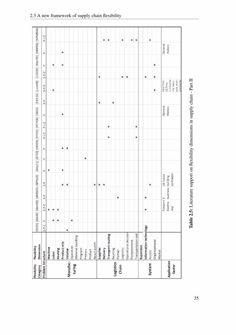
2.3 A new framework of supply chain flexibility
Tabl
e2.
5:L
itera
ture
supp
orto
nfle
xibi
lity
dim
ensi
ons
insu
pply
chai
n-P
artI
I
35
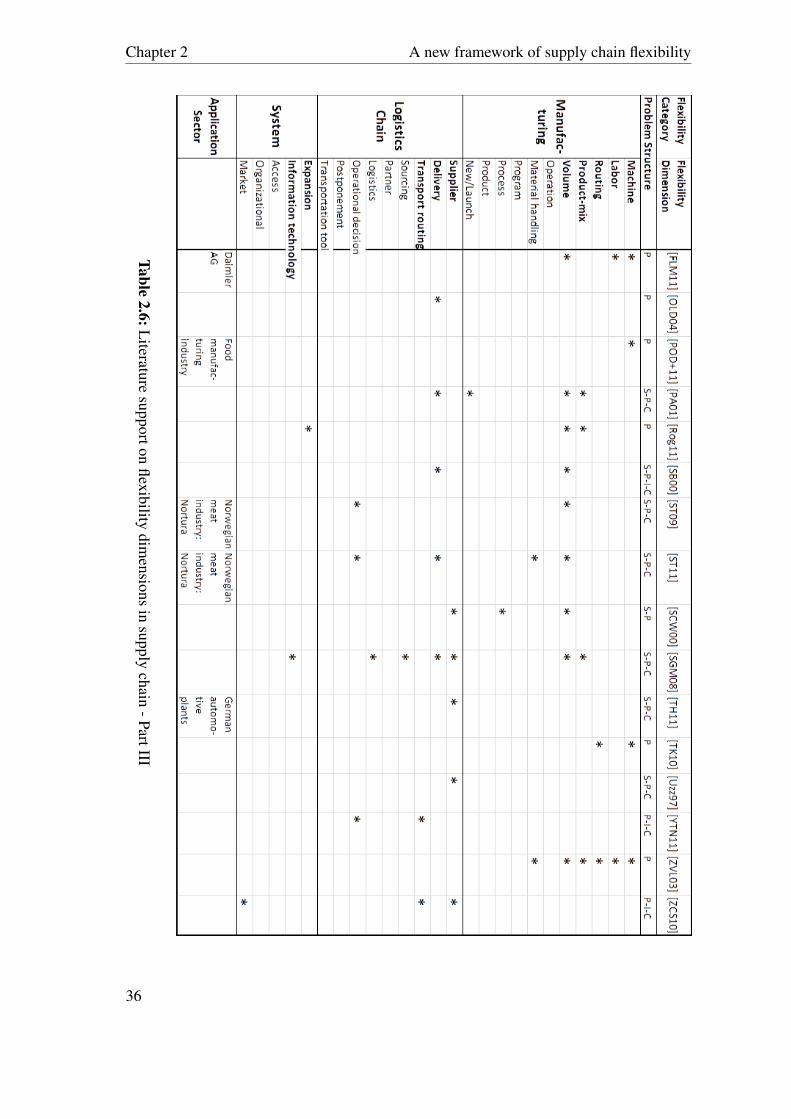
Chapter 2 A new framework of supply chain flexibility
Table2.6:L
iteraturesupporton
flexibilitydim
ensionsin
supplychain
-PartIII
36
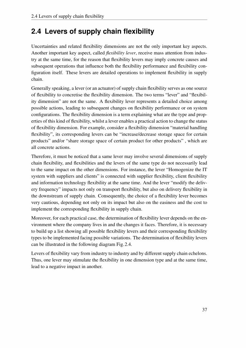
2.4 Levers of supply chain flexibility
2.4 Levers of supply chain flexibility
Uncertainties and related flexibility dimensions are not the only important key aspects.Another important key aspect, called flexibility lever, receive mass attention from indus-try at the same time, for the reason that flexibility levers may imply concrete causes andsubsequent operations that influence both the flexibility performance and flexibility con-figuration itself. These levers are detailed operations to implement flexibility in supplychain.
Generally speaking, a lever (or an actuator) of supply chain flexibility serves as one sourceof flexibility to concretise the flexibility dimension. The two terms “lever” and “flexibil-ity dimension” are not the same. A flexibility lever represents a detailed choice amongpossible actions, leading to subsequent changes on flexibility performance or on systemconfigurations. The flexibility dimension is a term explaining what are the type and prop-erties of this kind of flexibility, whilst a lever enables a practical action to change the statusof flexibility dimension. For example, consider a flexibility dimension “material handlingflexibility”, its corresponding levers can be “increase/decrease storage space for certainproducts” and/or “share storage space of certain product for other products” , which areall concrete actions.
Therefore, it must be noticed that a same lever may involve several dimensions of supplychain flexibility, and flexibilities and the levers of the same type do not necessarily leadto the same impact on the other dimensions. For instance, the lever “Homogenize the ITsystem with suppliers and clients” is connected with supplier flexibility, client flexibilityand information technology flexibility at the same time. And the lever “modify the deliv-ery frequency” impacts not only on transport flexibility, but also on delivery flexibility inthe downstream of supply chain. Consequently, the choice of a flexibility lever becomesvery cautious, depending not only on its impact but also on the easiness and the cost toimplement the corresponding flexibility in supply chain.
Moreover, for each practical case, the determination of flexibility lever depends on the en-vironment where the company lives in and the changes it faces. Therefore, it is necessaryto build up a list showing all possible flexibility levers and their corresponding flexibilitytypes to be implemented facing possible variations. The determination of flexibility leverscan be illustrated in the following diagram Fig.2.4.
Levers of flexibility vary from industry to industry and by different supply chain echelons.Thus, one lever may stimulate the flexibility in one dimension type and at the same time,lead to a negative impact in another.
37

Chapter 2 A new framework of supply chain flexibility
Figure 2.4: Determination of a flexibility lever
It is easy to understand that upstream flexibility levers in supply chain is strongly depen-dent on suppliers’ flexibility. The number of possible suppliers, the variety of suppliers,the contracts through which a firm can negotiate their concerning order quantity and vary-ing due date, and the connection between manufacturers and suppliers, are four importantelements to identity flexibility levers in upstream supply chain. Thus, for the supply orreplenishment part, flexibility levers in upstream supply chain can act as:
• Increase/Decrease the number of warehouses → Material handling and supplierflexibility
• Utilize the Cross-docking→Material handling and supplier flexibility
• Re-negotiate transport contract services→ Transport flexibility
• Mutualize the procurement with another company→ Supplier flexibility
• Homogenize the IT system with suppliers and clients→ IT and supplier flexibility
• Adopt RFID tags for products or pallets to improve the traceability and order prepa-rations→ IT flexibility
• Differentiate the delivery delay of clients→ Delivery flexibility
• ...
Meanwhile, most industrial requirements on manufacturing flexibility in a supply chainaim at two main flexibility dimensions: volume flexibility and product-mix flexibility.To tackle with the two requirements, a lot of levers are identified and proposed to solvethe problem using machine, routing, labor, process and other flexibility dimension tech-niques. Apart from that, the choice of lot-size, the internal configuration of production
38

2.4 Levers of supply chain flexibility
tool and variable lead time are all important parameters to identify flexibility levers inmanufacturing sites. Therefore, in manufacturing part of supply chain, flexibility leverscould be actions as follows:
• Train workers to be multi-skilling→ Labor flexibility
• Take overtime of the opening plant→Machine and labor flexibility
• Sub-contract one part of production goals→ Volume flexibility
• Increase or decrease the safety stock→Material handling flexibility
• Centralize the production planning→ Organizational flexibility
• Postpone the differentiating steps in manufacturing and assembly lines as late aspossible→ Routing and operation flexibility
• Rationalize the number of references to keep a simpler logistics → Product-mixand material handling flexibility
• ...
The principal concerns of downstream flexibility levers in supply chain concentrate onstorage capacity, delivery quantity, lead time and mix-delivery (the ability of a firm todeliver a variety of products at the same time), which are mainly related to dimensions likedelivery flexibility, transport routing flexibility, postponement, etc. Therefore, flexibilitylevers in distribution echelon can be identified according to parameters as: the numberof available transporters, the dependency or relation between product units and deliverypoints, delivery planning, lead time, etc. At the downstream of the supply chain, flexibilitylevers regarding distribution activities can act as:
• Increase the synergy between stores of various sizes
• Adapt delivery frequencies
• Deliver punctually and directly to sales point without passing through a distributioncenter or a warehouse
• Improve the visibility of controls to better manage HR
• Make possible changes to balance inventory levels between different warehouses
• Homogenize the IT system with clients
• ...
Before a flexibility lever is studied and implemented, one or several phenomenons mayserve as triggers for the corresponding lever. It is to be noted that a trigger may activateone or more flexibility levers at the same time, and an active flexibility lever incurs conse-quent effect on various aspects in supply chain. To understand this, consider a flexibilitylever “make use of storage space dedicated to certain products to store other products ”.
39

Chapter 2 A new framework of supply chain flexibility
One of its trigger can be the saturation of storage space dedicated to some types of prod-ucts. The implementation of this lever may accommodate changes on replenishment cycleand leads to positive effects such as better utilization of warehouses and less stock out.The negative effect is that the warehouse must be adapted to store and handle many typesof products at the same time. Not all products can be stored under the same conditions,so the adoption of this lever may incur risks of damaged or deteriorated products.
After the clarification of triggers and effects, the ease to implement a flexibility levershould be attentively investigated. First, the decision level of flexibility lever must beidentified, and its implementation, duration of implementation, associated Key Perfor-mance Index (KPI), relative costs and returns must be estimated. For instance, consider aflexibility lever in transport: “deliver punctually and directly to sales point without pass-ing a warehouse”. The triggers for it are multiple, such as the overstock of upstreamcenters, too long lead time, or even the risk of stock out in sales points. The lever lies inoperational decision level with a short implementation delay, but may require quite a longtime (duration) to be implemented. Thus, the cost of punctual and direct delivery is muchhigher than normal one, with possibly a small return on investment (ROI) if unit profit isnot too high. The KPI associated is Leadtime.
In this context, three teams of students in Ecole Centrale Paris have conducted their stud-ies by collecting useful information from partner firms, identifying a number of leversrespectively in upstream supply, manufacturing and distribution parts of supply chain.The five firm partners are Carrefour, Danone, Louis Vuitton, PSA and Vallourec of ChairSupply Chain in Industrial Engineering Laboratory of Ecole Cenrale Paris. The firstteam working on the upstream part of supply chain [LBGH13] has identified 52 leversin function of purchasing, warehousing, transportation, IT, conception, supplier, humanresource, forecasting and communication sectors. Another team working on the manu-facturing part of supply chain [LMM+13] has explored flexibility levers in machinery,human resource, factory, relation among factories, strategic decision and information sys-tem fields. The third team working on distribution [BCFS13] has investigated 49 leversseparately in warehousing, transportation, IT, strategic decision, sales outlet, demand,product-mix fields. Finally, the three teams have constructed a table each to help identi-fying the types of levers and clarifying its effects, its interrelation and its implementationin different criteria.
The three tables have been merged to a whole in order to constitute a helpful tool indecision making concerning flexibility levers in supply chain. A small extract of the tableis shown in Tab.2.7. The head of the table lists different criteria on temporal, control,effects, specificity and risk aspects, and the column on the left indicates lever type andthe lever itself in detail. From this piece extracted from the whole table, we can easily seethat for levers in type Transport and Stocks in Upstream supply chain, all the evaluationdescriptions and scores are marked in columns according to different criteria.
40

2.4 Levers of supply chain flexibility
Table 2.7: An extract of flexibility levers [BCFS13]
41

Chapter 2 A new framework of supply chain flexibility
2.5 Conclusion
Definitions and taxonomies of flexibility have been widely studied but no universal con-sensus has been achieved to date. In this chapter, we first propose a global view of supplychain flexibility and define it together with our industrial partners in Chair Supply Chainas: “La flexibilité est la capacité d’une organization à pro-agir et réagir face aux facteursexternes et internes, et à répondre à la variabilité de la demande avec la maîtrise du coût,sur un horizon donné”. That describes, the supply chain flexibility refers to the ability ofan organization to pro-act and respond to internal and external environment factors, andrespond to variability in customer demand over a given time horizon especially with costcontrol.
In order to construct a new framework of supply chain flexibility, we define the flexibilitydimensions and investigate their relations with environmental uncertainties and betweenthe dimensions themselves. On the basis of these conceptual studies and the existing lit-erature support for each dimension, we construct a framework of supply chain flexibilitybased on 8-dimension respectively on machine, labor, routing, product-mix, volume, sup-plier, delivery and transshipment flexibility, which are explicitly defined and analyzed inthis chapter.
Furthermore, to implement the flexibility in industrial world, we penetrate into the no-tion flexibility lever, which represents a detailed action and enables the concretization offlexibility dimension in a supply chain. Various aspects of flexibility levers are studied,such as triggers to activate them, durations, positive and negative effects for the rest ofsupply chain and their adequate or possible costs. These levers are of great value,whichmay serve as a reference to help firms identity whether it is worthy or not to implement aflexibility operation in their supply chains, that means, to make concrete flexibility deci-sions.
Throughout this chapter, we have dedicated to “defining the flexibility”. We finally outlinea concrete overview of conceptual and qualitative studies on supply chain flexibility, andconstruct a clear framework to identity the flexibility types and their operations.
42

3 Measurements andmethodologies on supply chainflexibility
This chapter addresses the measurement of supply chain flexibility from a quantitativepoint of view. This step is necessary to evaluate the possible actions to improve theflexibility, and/or to incorporate flexibility considerations in industrial production andtransportation planning problems. We first review the existing literature, and then, we usethe mechanical analogy method to assess the effective flexibility in a real life case andestablish the evaluation procedure to carry out this method in supply chain.
3.1 Introduction
Due to the hierarchical configuration of manufacturing system and the complexity of theentire supply chain, a focusable measurement of flexibility is always required for differentsystem properties, in order to meet the multidimensional supply chain flexibility.
It there is a generally accepted assessment system for measuring supply chain flexibility,it would be needed to be ideally applicable cross-industries, and be able to release com-prehensive and comparable results. Comprehensive research in technical literature hasshown a great number of methods for the measurement of flexibility across the manufac-turing activities, but a bit less in the supply chain. This implies on one hand a continuallygrowing interest in the subject, on the other hand the lack of a generally accepted evalu-ation and optimization methodology. However, studies show another good trend, that iswith extensive descriptive, empiric and survey documents in literature, some quantitativeresearches have come up in the last decade, in order to add quantifiable values to differenttypes of supply chain flexibility.
As a result, existing methods can be generally classified into three categories:
• Conceptual and survey researches, which preserve a great part of literature on sup-ply chain flexibility. This kind of articles often gives descriptive analysis, or collects
43

Chapter 3 Measurements and methodologies on supply chain flexibility
traversal questionnaires among different industrial sectors and penetrates into dif-ferent internal activities in the studied supply chain echelon to draw conclusions.For instance, papers of [SS90, KM99, Lee04, Arv05, TT07] are all in this category.
• Development of measures and the evaluation of detailed flexibility dimensions per-taining to the supply chain activities, which take a small part of existing studies.Studies in this field as [AMMC05, Rog11, WWL08, Bay09, FLM11].
• Methodologies that investigate a rough or total flexibility performance without sub-division in precise dimension of flexibility, or, encompass some flexibility issuesor considerations when exploring other industrial problems (e.g. supply chainmanagement skills, production planning, facility location optimization, ...). Theseworks provide an important part of existing contributions, as work in [XN09, TK10,ZCS10]. Uncertainty term is frequently used in this category, for instance, Vi-dal and Goetschalckx [VG00] incorporate uncertainty considerations into a mixedinteger linear program with some specific stochastic constraints, such as supplierreliability and on-time performance.
Comprehensive descriptive, analysis and survey results are principally mentioned andpresented in the previous chapter in sec.2.2. In this chapter, we pay attention mainlyto the second and the third categories, whose studies establish mathematical formulas,models and/or develop effective algorithms to measure and solve problems with supplychain flexibility concerns.
3.1.1 Evaluation of dimensions of supply chain flexibility
Compared with enormous conceptual work talked about in sec.2.2, quantitative studiesregarding supply chain flexibility start to emerge during the last decade. Different authorshave proposed proper measures and methodologies to quantify the flexibility in each levelof the supply chain system. Among these methods, the volume flexibility and product-mixflexibility defined by our new classification, are most studied in manufacturing system.
Different methods exist to incorporate the flexibility dimensions into an optimization ofproduction or distribution problems. Most of the studies focusing on some particularflexibility dimensions, are complicated and impossible to present briefly the flexibilitymeasure out of the entire model separately. However, Rogalski [Rog11] proposes a goodmethodology evaluating the volume, mix and expansion flexibility, in which each of themare incorporated with very simple formula and especially, can be expressed separatelywithout interfering into the analytical model in details. Thus, it is more appropriate tobe presented here to show how to evaluate flexibility dimensions in a supply chain. It ispresented in the following paragraphs.
44

3.1 Introduction
Volume flexibility
Volume flexibility is always related to the manufacturing system’s capacity. It implies thefirm’s competitive potential to change production volume in order to meet market demandwhile remaining profitable. From this definition, we can state that, the profitable limitsof the system with the considered period must be respected. Hence, two parameters areimportant [Rog11]:
• Break-even-point: the manufacturing quantity at which the revenues cover the totalcosts (fixed and variable costs) and the resulting profit is zero.
• Maximum capacity: the biggest possible capacity the system is able to reach wherestill profitable. It is determined by the technical details of the manufacturing facilityand organizational measures like flexible man-hour models, e.g., overtime or multi-shift.
The range between the Break-even-point and Maximum capacity is called the FlexibilityRange, during which the system remains economical while varying the production output.This is expressed as a relative figure (Fig.3.1), with a flexibility range representing thevolume flexibility, originally in black.
Thus, we could simply calculate the Flexibility Range as xMAX (S)− xBE (S), where Sdenotes a manufacturing system or one system object, and xBE (S) denotes the Break-even-point. The Flexibility Range is an absolute value to characterize the dimension ofthe economical, object-dependent part of manufacturing. Here the “system object” refersto the studied object in the manufacturing system, which can be a workshop, a productionline, a production site, any part or total line of the manufacturing site, etc.
In order to compare different system objects, this flexibility range has to be put in arelationship with the Maximum capacity, and the volume flexibility can be formulated:
Fvolume (S) =xMAX (S)− xBE (S)
xMAX (S)·100% (3.1)
As a result, the bigger the relative deviation between the Break-even-point and Maximumcapacity, the higher the volume flexibility for the system or the system object.
Product-mix flexibility
Product-mix flexibility disposes the ability to switch between several products without in-fluencing negatively the optimal system profit. It is often measured by the cost and time of
45
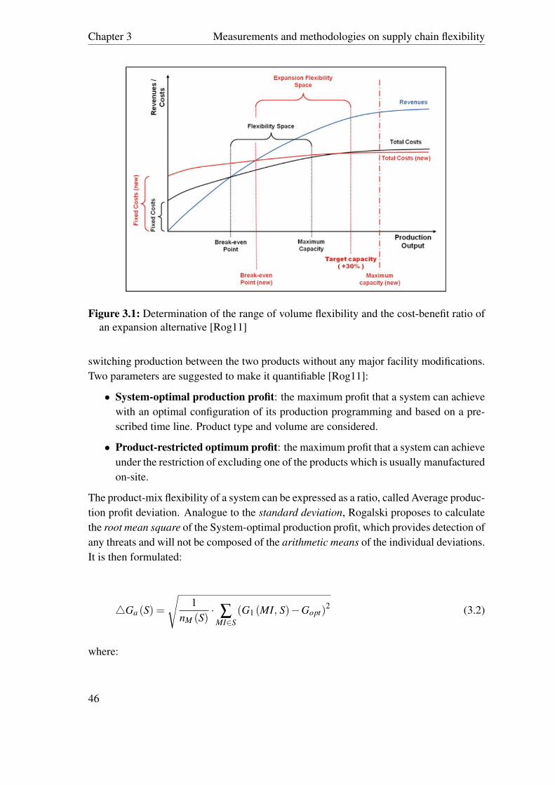
Chapter 3 Measurements and methodologies on supply chain flexibility
Figure 3.1: Determination of the range of volume flexibility and the cost-benefit ratio ofan expansion alternative [Rog11]
switching production between the two products without any major facility modifications.Two parameters are suggested to make it quantifiable [Rog11]:
• System-optimal production profit: the maximum profit that a system can achievewith an optimal configuration of its production programming and based on a pre-scribed time line. Product type and volume are considered.
• Product-restricted optimum profit: the maximum profit that a system can achieveunder the restriction of excluding one of the products which is usually manufacturedon-site.
The product-mix flexibility of a system can be expressed as a ratio, called Average produc-tion profit deviation. Analogue to the standard deviation, Rogalski proposes to calculatethe root mean square of the System-optimal production profit, which provides detection ofany threats and will not be composed of the arithmetic means of the individual deviations.It is then formulated:
4Ga (S) =
√1
nM (S)· ∑
MI∈S(G1 (MI, S)−Gopt)
2 (3.2)
where:
46

3.1 Introduction
nM (S) Number of different kinds of products M of system object S
G1 (MI, S) Product-restricted profit optimum of product MI in system object S
Gopt System-optimal production profit of the whole system
4Ga (S) Average production profit deviation in system object S
In order to compare different system objects or different production systems, the Averageproduction profit deviation must be put in a relationship to System-optimal productionprofit. The flexibility of product-mix can be formulated:
FMix (S) = 1−4Ga (S)Gopt
·100% (3.3)
From this formulation we can see if there exists only one single-product fabrication, theproduct-mix flexibility will take the value of 0. Subsequently, the value 1 stands for thecomplete product-mix flexibility.
Expansion flexibility
Expansion flexibility is a long-term flexibility and related to the easiness of adding moreor new capacity to an existing system. Consequently, it is assumed to be quantity-relatedto the maximum capacity in the previous determined phase. Before the determination ofthe expansion range, we first calculate the target capacity for system object of a manufac-turing system. This target capacity has to be multiplied with the maximum capacity thatrelates to product-mix flexibility in the previous phase.
TC (S) = (1+ e) · xMAX (S) (3.4)
where:
TC (S) Target capacity of system object S
xMAX (S) Maximum capacity for system object S
e Given expansion capacity of system object S in per cent, specified by the user
Depending on the system object concerned, a specific alternative problem that maximizesthe capacity can be solved using a simplex-algorithm. Afterwards, the alternative-specificBreak-even-point, noted as xBEA , has to be calculated using the same logic during the de-termination phase of volume flexibility. The calculation procedure for the whole system
47

Chapter 3 Measurements and methodologies on supply chain flexibility
and for subsystems should be distinguished, and for each valid alternative point, the re-lated adequate linear programming problem have to be slightly reformulated and solved.Afterwards, with the knowledge that the original flexibility range may arise when calcu-lating the volume flexibility, it’s time to consider the expansion flexibility.
The expansion-based flexibility range depends on the Break-even-point of the individualexpansion alternatives, which is colored in red in Fig.3.1. The original flexibility rangeof the system is in black, between the original Break-even-point and Maximum capacitygenerated within the limits of the Volume flexibility.
Thus, the expansion-based flexibility range for different system objects can be expressedas TC (S)− xBEA (S). The closer an alternative comes to reaching this point, the largerits expansion-based flexibility range and therefore the bigger its influence on the Cost-Benefit ratio of the system.
Thus, the expansion flexibility for different system objects can be calculated from:
FExpansion (S) =TC (S)− xBEA (S)xMAX (S)− xBE (S)
·100% (3.5)
As a result, the expansion flexibility of a manufacturing system is dependent on the ex-pansion alternative with this highest Cost-Benefit ratio. The bigger the relative deviationbetween its Break-even-point and its Target capacity, the more flexible expansion the sys-tem.
Apart from the evaluation of several particular flexibility dimensions, Rogalski also de-fines a Cost Accounting Reference Frame in his book [Rog11]. These flexibility dimen-sions are integrated into the frame in order to form and perfect a complete methodology.
Among the existing literature, volume flexibility and product-mix flexibility have receivedvast attention in the literature on manufacturing system flexibility studies. Goyal andNetessine [GN11] work over a single firm with two products, facing the choice of select-ing one of the four strategic flexibility technologies: D (not flexible), V (volume flexible),P (product-mix flexible) or V P (both volume and product-mix flexible). They formulatefour models whose objective functions with or without volume or product-mix flexibletechnologies and highlights that adding the P to V is not always beneficial. They arguethat the volume flexibility value is a function of demand correlation between products, andthe product-mix flexibility value decreases in demand correlation. They then underscorethe necessity of analyzing volume flexibility with more than one product and emphasizethe opposite with product-mix flexibility.
In a smaller supply chain scale, machine flexibility is the most studied in manufacturingworkshop. Baykasoglu [Bay09] propose a new approach based on digraph theory and ma-
48

3.1 Introduction
trix algebra to quantify machine flexibility. Wahab et al. [WWL08] provide a generic ap-proach to measuring machine flexibility in manufacturing systems. Francas et al.[FLM11]propose a two-stage stochastic program with recourse to study the investments on laborand machine capacity, under uncertain demand and a given network configuration whileanticipating the deployment of labor flexibility. They investigate the impact of labor flex-ibility on machine and labor capacity and its interplay with machine flexibility, and showthat personnel transfers are more effective in larger manufacturing networks.
3.1.2 Measures and methods of supply chain flexibility
Probabilistic approach: Penalty of Change method (POC)
This is a general probabilistic measure used to measure flexibility of a manufacturingsystem, which determines the flexibility by its sensitivity to changes. This method canbe easily extended to whole supply chain. And, the lower the sensitivity is, the higherthe flexibility is. High flexibility or low sensitivity to changes can bring advantages toa supply chain system at least in product-mix, operation and volume flexibilities in ourdefined framework.
The measure is based on evaluation of additional costs in case of potential change, calledpenalty cost, and the probability of potential change. It works as an index “Penalty ofChange” (POC) [Chr96], where change is a transition from one “state” to another. Ifthe considered change within a system can be solved and handled without incurring anyfurther costs, we say the system holds maximal flexibility so that the POC-value is zero.Chryssolouris [Chr96] goes back to the concept of Event Tree, with what he calculatespenalty costs on the basis of occurrence probabilities of future scenarios.
Both penalty and probability can be viewed as functions of a discrete random variableX , which represents potential change. For instance, in three possible states A, B and C,the possible values of X are X1 (A,A), X2 (A,B), X3 (A,C), X4 (B,A), X5 (B,B), X6 (B,C),X7 (C,A), X8 (C,B), and X9 (C,C). Here, the combination (A,A) indicates the system staysin the same state A, and (A,B) refers to a transition of system state from (A,A) to (A,B).The penalty of change (POC) can be then defined as:
POC = ∑i
Pn(Xi) ·Pr (Xi) (3.6)
where:
Xi the ith potential change
49
Chapter 3 Measurements and methodologies on supply chain flexibility
Pn(Xi) penalty of the ith potential change
Pr (Xi) probability of the ith potential change
The calculation of POC can be also viewed as a procedure of single-attribute decisionmaking under uncertainty. If Xi stands for possible future scenarios, Pn(Xi) representsthe attribute values for each future scenario and Pr (Xi) interprets the probabilities ofoccurrence of the scenarios.
Furthermore, consider the most general case that a system may not process a finite set ofdiscrete state-changes but a continuous range of state-change couples, the formula 3.6 canbe changed to a continuous integral form with continuous distribution Pn(X) and Pr (X)
in function of continuous variable X . Consequently, the scenario with the lowest cost isconsidered to be the best.
The flexibility evaluation on the basis of the “Penalty of Change” is possible to include allprocesses from workplace to plant and supply chain scenarios as well. It specially makessense for the evaluation of different options or expansion alternatives in regard to costs.The first crucial disadvantage is the distinct dependence on occurrence probabilities ofscenarios and corresponding costs. The second default is one must provide a completelist of the possible changes and make a right anticipation of all the potential costs againstthe changes. This need of data collection and especially the anticipation of data, may bequite a difficult requirement for firms, which limits the application of the measure.
Alexopoulos et al. [AMMC05] present a study of flexibility for the punching departmentin a commercial refrigerators manufacturing system, where three technology solutions forthe punching department under different sets of production requirements are considered.They investigate the flexibility of punching manufacturing system with the use of POCmethod, and give a good picture of the flexibility characteristics for alternative solutionsof the punching department.
DCF analysis: Design of Systems for Manufacture (Desyma)
Design of Systems for Manufacture (DESYMA) is a flexibility evaluation method devel-oped at the Greek University of Patras to assess the flexibility of a manufacturing systemstatistically. With different demand insecurities, it refers to the evaluation of alternativedesign solutions of manufacturing systems.
In this method, flexibility is considered by using a “Discounted Cash-Flow” (DCF) anal-ysis. This is a statistical analysis of discounted estimations of the Cash-Flow, where allfuture cash flows are estimated and discounted to give their present values (PVs) - thesum of all future cash flows, both incoming and outgoing, is the net present value (NPV),which is taken as the value or price of the cash flows in question. Present value may also
50
3.1 Introduction
be expressed as a number of years’ purchase of the future undiscounted annual cash flowsexpected to arise.
Afterwards, the life cycle time of a considered production system is evaluated with dif-ferent market scenarios in a certain time period. Based on the distribution of DCF values,the flexibility evaluation in the supposed market environment occur afterwards. The cor-relation between the DCF and the flexibility implies that, the smaller the distribution ofDCF values are, the more flexible the production system is, and the more stable life cyclecosts are [AMMC05].
The DCF can be calculated for each market scenario and the spread of the DCF scores mayrepresent the flexibility of the system in the given market environment. Consequently, thedispersion of DCF-values leads to a kind of “collective flexibility” and involves costsfor different market scenarios, thus, some particular costs (for measuring adaptation, forinstance) can be evaluated cross-industrially on the basis of sales expansion.
In another aspect, the scenario related part of this method turns out to be disadvantageous,and, the quality of results depends on the subjective user’s judgment. The long-termexpansion flexibility of a production system can be deduced from DESYMA method,whilst the volume and product-mix flexibilities are hard to deduce from this method.
Alexopoulos et al. [AMPC07] propose a backward optimization algorithm implementedin Visual Basic for Excel, as a part of the overall DESYMA method. Both expansionand contraction of a system are considered in this paper, using DCF values to comparethe flexibility of alternative manufacturing systems. Results prove that this algorithmreleases accurate solutions and runs faster than normal DESYMA design method. Anapplication of this method to a production investment case study is carried out with dataderived from the automotive industry.
Dynamic modeling approach: Mechanical vibration analogy
A production line can be viewed as a mechanical vibration mechanism [APM+08]. Thedemand expressed in quantities of products at a certain production duration, can serve asthe input data to the adequate mechanical mechanism; the delivery expressed in quantityof products and lead times, can be interpreted as the output of the mechanical mechanism.This kind of analogy is cited as the ζ -analogy method [Chr96], where ζ indicates a di-mensionless damping factor of the mechanical system. Hence, the damping factor ζ isconsidered to represent the insensitivity to environment change. This approach is furtherdescribed in details in sec.3.2.1.
FLEXIMAC
Other than the traditional mechanical system analogy, another way of evaluating flexibil-ity is the FLEXIMAC method. It overlaps to some degree the early ζ -analogy method,
51

Chapter 3 Measurements and methodologies on supply chain flexibility
and goes back to the analogy of dynamic properties between a mechanical system and aproduction system. The ability to react to potential changing in a mechanical system ischaracterized by the damping factor ζ , that can be deduced and calculated under certaincircumstances using a transfer function [APM+07]. The same logic applies to a produc-tion system, where the system flexibility can be evaluated with the ability of reaction inregard to the dynamic input excitations.
The input could be processing time of a production system, which is necessary to producea required varying quantity and type of products. The output may be represented as actualflow time, which is normally longer than the supposed processing time, due to variablewaiting time during the production with incidences such as accidents, lack of raw materi-als, lack of human resources, etc. In the ideal case, input and output should be identicalwithout delay.
It is necessary to divide the predicted period length in equal time intervals, and collectthe data on processing time as well as the flow time. The concrete FLEXIMAC valueis calculated from the arithmetic mean of the ten highest amplitudes in the spectrum, asexpressed in formula 3.7, where Qi is the amplitude corresponded to the eigen frequency.The higher the FLEXIMAC value for a production system is, the more flexible it is, theless sensitive towards input variations.
FLEXIMAC =110
10
∑i=1
(1
2Qi
)(3.7)
The great advantage of FLEXIMAC-method is the non requirement of explicit internalvariables and data gatherings. The only need is input and output data, neglecting all thesystem and organization configurations. These relevant data can be easily gathered fromworking data or Enterprise Resource Planning (ERP) Systems. The second advantageis its independence from subjective assessments and reference scenarios, as it is trans-formed by a mechanical view. Furthermore, evaluation of flexibility can be executedcross-industrially on all relevant levels, starting at the machine level, workplace level tothe point of the factory and supply chain level.
There are also disadvantages. In applying this method, concrete conclusions regardingexpansion flexibility is completely impossible, because it disregards completely the macromeasures such as total costs, total revenue to integrate in the method, so that the evaluationof volume and product-mix flexibility are hard to derive or only possible in a limited way.With this great disadvantage, the mechanical analogy method can evaluate the flexibilityof the system only in a general sense, rarely for a special small flexibility dimension.
52
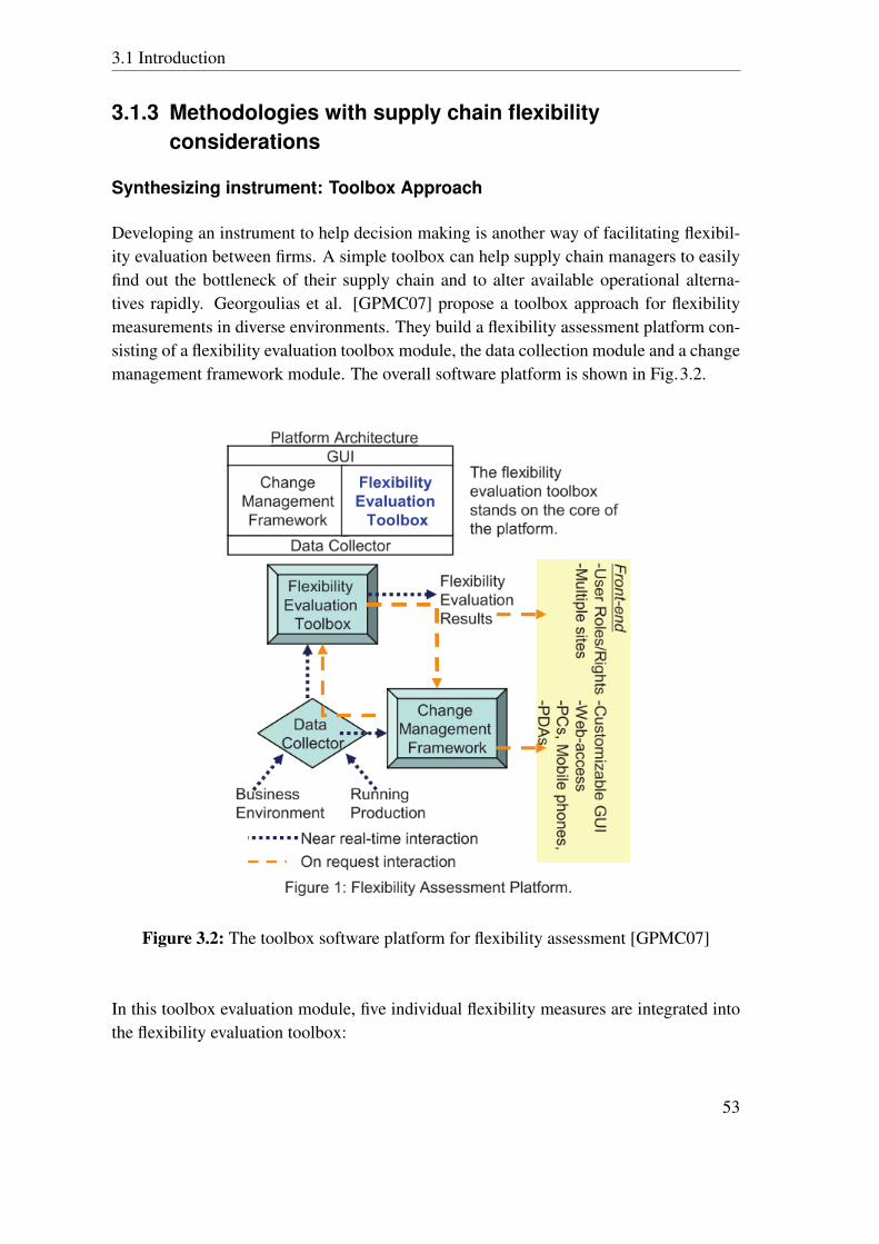
3.1 Introduction
3.1.3 Methodologies with supply chain flexibilityconsiderations
Synthesizing instrument: Toolbox Approach
Developing an instrument to help decision making is another way of facilitating flexibil-ity evaluation between firms. A simple toolbox can help supply chain managers to easilyfind out the bottleneck of their supply chain and to alter available operational alterna-tives rapidly. Georgoulias et al. [GPMC07] propose a toolbox approach for flexibilitymeasurements in diverse environments. They build a flexibility assessment platform con-sisting of a flexibility evaluation toolbox module, the data collection module and a changemanagement framework module. The overall software platform is shown in Fig.3.2.
Figure 3.2: The toolbox software platform for flexibility assessment [GPMC07]
In this toolbox evaluation module, five individual flexibility measures are integrated intothe flexibility evaluation toolbox:
53
Chapter 3 Measurements and methodologies on supply chain flexibility
• Penalty of Change
• ζ - analogy method
• Desyma
• FLEXIMAC
• Reaction-time analogy
The platform firstly sorts the enterprise level criteria and the flexibility types that couldbe measured, then examines the required data complexity from current IT systems toaggregate possible flexibility measurements of lower levels. The easiness of application ofeach flexibility measures is noted and recommended to import to the change managementframework. The approach overcomes the limitation of using a single flexibility measure,and provides the opportunity for managers to select from a broader set of several flexibilitymeasures.
Simulation based on Petri nets
Petri nets are a class of modeling tools originally proposed by Petri [Pet76]. A Petri net isa directed graph consisting of places, transitions, and arcs. The nodes denote transitions,representing events that may occur, signified by bars or boxes; the places are drawn ascircles, representing possible states or conditions. Arcs run from a place to a transition orvice versa, never between places or between transitions. The relationships between placesand transitions are linked by a set of arcs in either direction. The places from which anarc runs to a transition are called the input places of the transition; the places to whicharcs run from a transition are called the output places of the transition. And, the dynamicbehavior of the system can be represented using tokens which graphically appear as blackdots in places.
Simulation of manufacturing activities or supply chain activities can provide estimation ofthe required times for a system to adapt to various environmental disturbances. The timecan be interpreted as a kind of responsiveness, and can be used as flexibility measures[BS88].
Furthermore, a flexible manufacturing system (FMS) is a discrete-event system, wherea discrete number of parts or components are processed and assembled by controlledmachines, computers or robots and a number of resources shared to reduce the productioncost. Viswanadham et al. [VNJ90] investigate the use of Petri net (PN) models in theprevention and avoidance of deadlocks in flexible manufacturing systems, and propose aPetri net-based on-line controller.
Tüysüz and Kahraman [TK10] present a complex time critical and dynamic system, mod-eled in stochastic Petri nets with fuzzy parameters for a flexible manufacturing cell con-taining nine places and five transitions. El-Tamini et al. [ETAMA12] choose Petri nets
54
3.1 Introduction
for measuring and analysis of the FMS performance, integrating machine flexibility androuting flexibility in their model. The authors conducted an example FMS in its Petrinet model, AweSim model (Visual Slam AweSim to run simulations) and a mathematicalmodel. They conclude their method works well for the studied case, but for a complexsystem, they suggest using simulation techniques instead of mathematical reformulation.
Other models and methodologies in supply chain flexibility
Chan et al. [CBW07] provide a simulation study for the flexible manufacturing sys-tem, using Taguchi’s method to analyze physical and operating parameters with flexibilityrange. The Taguchi’s method [Ran90] allows the analysis of experimental results to es-timate the relative contribution of individual factor and interactions with other factors, inpercentages. The results show that an increase of routing flexibility (RF) may not alwayslead to expected benefits, and could be counterproductive under certain environment, ifvariations are above certain limits. The conclusion is useful for decision maker to distin-guish the flexibility level up to which can be increased in a set of varying physical andoperating parameters, and still retains the profitability.
An economic evaluation model across the entire supply chain is proposed by Gong [Gon08].The author adds systemically machine flexibility, labor flexibility, routing flexibility andinformation technology to construct the supply chain model. The objective function leadsto a probabilistic average profit, as an economical index. These dimensions of flexibilityare constructed and integrated by adding specific probabilistic distributions to correspond-ing factors. For instance, they use βi to represent the time with a probability distributionneeded by team j to finish one unit of product i, which is multiplied with the team workeroutput to form a labor capacity, which represents the labor flexibility. Results are obtainedthrough Matlab. The author provides a sensitivity analysis as well, which supports thatonly several flexibility dimensions in certain teams, certain products and certain routesare the main factors that affect the most system flexibility.
Swafford et al. [SGM08] conduct an empirical study to determine the effect of IT inte-gration on the SC process-specifically in regards to SC flexibility and SC agility. Theirquestion is mainly about “How IT flexibility can influence the supply chain flexibility as awhole?” Based on data analysis, they conclude that IT integration improve SC flexibilityand SC agility as well, but argue that SC flexibility and agility are two distinct concepts.They use Confirmatory Factor Analysis (CFA) as the tool to examine the relationshipbetween flexibility types. CFA is used to examine whether the proposed measures of aconstruct are consistent with a researcher’s understanding of that construct (or factor),mostly used in social research. Thus, the objective of CFA is to test whether the data fit ahypothesized measurement model [Jör69].
55

Chapter 3 Measurements and methodologies on supply chain flexibility
Apart from studies on information dimension, Liu and Cetinkaya [LÇ09] adopt a gametheoretic modeling approach to explore the supply contract flexibility from the perspec-tive of a bilateral setting, and address on leadership between the two sides. The au-thors consider a buyer-driven policy and derive an optimal methodology with informationasymmetry for three different types of contracts: “under a two-part linear contract, theimpact of information asymmetry depends on the buyer’s estimation accuracy; a two-partlinear contract, it depends on the buyer’s estimation accuracy; a two-part non-linear con-tract, it increases the buyer’s profit margin.” They conclude that the buyer-driven channelshows more efficiency than supplier-driven underone-part linear contract, and the part-ner without accurate information may not benefit from having leadership even for a goodtwo-part non-linear contract, in other words, sometimes one can forfeit the leadership inthe supply-buy relation and still gain higher profit.
Xu and Nozick [XN09] propose a supply chain design model for supplier selection. Theyconsider supplier capability disruptions to be a risk to the SC process, look for good choicebetween taking a trade-off based on cost and the risks of selecting suppliers in variouscategories, or taking the optional contracts. Erhan Kesen et al. [EKD10] consider the casewhere the buyer releases a fixed period replenishment order to the supplier under a supplycontract in three parameters: (i) supply price per unit (ii) minimum order quantity and (iii)order quantity reduction penalty. Their work suppose there is no penalty for not placingan order. They then suggest a model to select supplier by minimizing the procurementplus lost sales cost. A key buyer decision is Qlost , the order or replenishment quantitylevel below which no order is placed and sales are lost. Authors consider the flexibility ofinventory replenishment under a contract, while optimizing costs and avoiding inventoryrisks based on the optimum value of Qmin (minimum order quantity) and Qlost .
Zhu et al. [ZCS10] work on a two-stage serial supply chain in which a retailer and hissupplier are operating in make-to-stock environments, with the uncertain demand problemfaced by retailers. Their model consider a decentralized supply chain with a so-calledperiodic flexibility, where retailers could order any quantity in one period of the cycle,based on contract conditions that they would receive a fixed quantity from the supplierduring other periods. The results demonstrate that periodic flexibility improves the supplychain performance by about 11% on average and highlight the centralization control. Thisperiodic flexibility can be viewed as a supplier flexibility, the sourcing quantity flexibilityand a delivery flexibility. Moreover, the information communication plays an importantrole in their case. Chan and Chan [CC10] propose a two-echelon SC inventory cost modelto study the supplier capacity and delivery flexibility in a make-to-order (MTO) supplychain. The work employes an agent-based simulation to get the results, and also concludeboth the flexibility for MTO and the adaptability would provide better cost than order-up-to policy model costs.
Das [Das11] tries to develop models to integrate volume, product mix, distribution and
56

3.1 Introduction
supply flexibility in a strategic level. A mixed integer supply chain planning model isthen proposed as a way of addressing demand and supply uncertainty, as well as consid-ering various market scenarios. Based on the product mix flexibility, the model selects anoptimal number of products from fast moving and extended product range options, thenconfirms a quick response to a changing marketplace by considering transport and supplylead time along with the stock out probabilities, with supply and distribution flexibil-ity. The author proposes a scenario-based stochastic approach for estimating the demandincrease towards capacity flexibility planning, and provide a step-by-step procedure forsolving the model and applying the flexibility measures.
57
Chapter 3 Measurements and methodologies on supply chain flexibility
3.2 Application of the mechanical analogy methodto a practical case
3.2.1 Introduction on mechanical analogy method
3.2.1.1 General introduction
In this method, a manufacturing system can be viewed as a mechanical system, whoseinput is excitation force and the output is displacement or the movement of the mechanicalsystem. Inside the mechanical vibration box, a simple mechanism generally consists ofan elastic spring, a damper, a mass and their oscillatory interactions. In the same logic, amanufacturing plant system is composed of several manufacturing resources (machines,labor, raw materials, ...) and production activities. Outside the manufacturing systemor a workshop in a manufacturing system, the input may often be the fabrication orderexpressed in quantities of products with a certain estimated processing time; the outputcan be the finished order expressed in quantity of products and real flow time. This isshown in the left part of Fig.3.3.
Nevertheless, the analogical notion can be easily extended to the whole supply chain andapplied to different echelons in/of a supply chain. For example, the analogical input datato a supply chain or to an echelon of supply chain can be symbolized as client demand,which could be expressed in quantities of products with estimated lead time or an agreeddue date; the output can be presented as delivery operations expressed in quantity ofproducts and real delay time. This is shown in the right part of Fig.3.3.
For a mechanical vibration system, excitation force and mechanism displacement varyover time, and so do the fabrication orders and delivered orders of an manufacturingsystem. Therefore, a manufacturing system may exhibit strong dynamic behavior, whichis difficult to be described with mathematical curve and often nonlinear. On the otherhand, flexibility is well defined for a simple dynamic mechanical system, representing itsinsensitivity to external excitation. Thus, the flexibility of manufacturing system can beobtained with the help of the appropriate mechanical damping factor [Chr96].
Moreover, by studying properties of a supply chain, we consider this damping conceptable to be extended to whole supply chain and could be adapted to different echelons in asupply chain. The flexibility of supply chain system can be also obtained with the help ofmechanical damping factor, as a supply chain can be also viewed as a system composedof several supply chain resources (suppliers, production plants, transportation vehicles,...) linked by several supply chain operation activities, as well.
58

3.2 Application of the mechanical analogy method to a practical case
Figure 3.3: Analogy between a manufacturing and a mechanical system [Chr96]
3.2.1.2 Methodology
Before stepping into the detailed methodology, we start by identifying a simple mechani-cal oscillatory system.
All concrete bodies possessing mass and elasticity in the world are capable of vibration,that can be further distinguished into two vibration classes - free and forced vibration[TD98]. Free vibration takes place when a mechanical system oscillates under the actionof inherent forces in system itself, and leaves the body vibrate alone at one or more naturalfrequencies, which are linked with the intrinsic properties established by the distributionof its mass, stiffness and damping (if it has a damper). Forced vibration takes place underthe excitation of external forces, where the body is forced to vibrate at the excitationfrequency (if the excitation exhibits a frequency).
A mechanical system may oscillate in different modes, described by its number of in-dependent coordinates, called degree of freedom. For example, a rigid dust floating in avacuum room is capable to vibrate in three degrees of freedom. Besides, all oscillatorymechanism subjects to damping effects to some degree, because there exists always theenergy dissipation by heat radiation, friction and other resistances.
For the mechanism of a single-degree freedom with known mass, elasticity and dampingproperties, the damping factor can be easily calculated, noted as ζ . The following expres-sion shows the relationship between damping factor and other attributes of the mechanical
59

Chapter 3 Measurements and methodologies on supply chain flexibility
oscillator system :
ζ =12
√c2
km(3.8)
where:
c the damping of the mechanical system
k the stiffness of the mechanical system
m the inertia of the mechanical system
ζ the damping factor representing the system’s ability to respond to changes inthe excitation
The mass is considered to be measured in SI system [Cox58] as kilograms kg or g. Thelinear spring follows Hook’s law[Hoo78], Fk = kx, where the stiffness k is measured innewtons/meter n/m. A simple viscous damping is described proportionally to the velocityFc = cx, where the damping coefficient c is measured in newtons/meter/second n · s/m.The damping factor ζ is dimensionless.
Naturally, if we make use of nominal attributes to achieve the analogy between mechani-cal oscillator and corresponding supply chain, the four attributes become as follows:
c the damping of the supply chain system
k the stiffness of the supply chain system
m the inertia of the supply chain system
ζ the damping factor representing the system’s ability to respond to changes inthe input/excitation
For a mechanical oscillator system, the damping factor ζ can be estimated from the fre-quency spectrum in an approximate way, as follows:
ζ ≈ 12Q
(3.9)
where Q is the amplitude corresponding to the fundamental natural frequency in its fre-quency spectrum, which will be detailed in the following paragraphs. This is the corerelation of our method.
Consider any mechanical system solicited by a time-varying force f (t) with f (t = 0) =F , and reacted by a movement x(t). The differential equation that describes the vibration
60

3.2 Application of the mechanical analogy method to a practical case
motion of simple-degree system undergoing the excitation f (t) at time t = 0 is:
mx(t)+ cx(t)+ kx(t) = f (t) (3.10)
recall:
m the mass coefficient of the mechanical vibration system
c the viscous damping coefficient of the mechanical vibration system
k the stiffness coefficient of the mechanical vibration system
x(t) the displacement of the mechanical vibration system
x(t) the velocity of the mechanical vibration system
x(t) the acceleration of the mechanical vibration system
The response x(t) of a damped single degree of freedom mechanical system subjectedto an impulse excitation at time t = 0 could be then deduced and expressed by Eq.(3.11)[Tho93](recall f (t = 0) = F):
x(t) =F
mω√
1−ζ 2e−ζ ωt sin
√1−ζ 2ωt (3.11)
where:
ω the circular frequency of the mechanical system, given by ω =√
km
ζ the damping factor representing the mechanical system’s ability to respondto changes in the input, given by ζ = c
2mω
When an excitation f (t) is applied at time t = 0+, the initial velocity of movement isgiven by relation:
x(0+)=
Fm
(3.12)
Thus, if the initial velocity and the force are all known, the mass can be directly estimated.That means the nominal value m of the supply chain system, can be determined by thefollowing:
m =F
x(0+)(3.13)
61

Chapter 3 Measurements and methodologies on supply chain flexibility
In order to numerically record the time-varing force and the displacement of the mechan-ical system, the couple x(t) and f (t) can be both discretized and sampled in length N:
fn = f (tn) xn = x(tn) , n = 0, 1, 2, ...N−1 (3.14)
where tn = n4, 4 is the sampling interval, as what we have presented in sec.3.2.1 tostudy its transfer function in the frequency spectrum.
The transfer function between the input and output of a supply chain system could char-acterize the way the system responds to changes in the input, such as variations in ordersof different products in different volumes and due dates.
This transfer function can be expressed in the frequency domain. For a continuous rangeof frequencies, the variable ω denotes the circular frequency in radians/sec. For the DFT(Discrete Fourier Transforms) series, the discrete frequencies are all multiples of a specificfrequency ω0, called the fundamental frequency. Therefore, the transfer function of thesystem can be expressed as:
H (ω) =X (ω)
F (ω)(3.15)
where :
ω given by the relation ω ∈ hω0 | h = 0, 1, 2, ...N−1, set ω0 = 2π/N for xn
of length N.
X (ω) the Discrete Fourier Transforms (DFTs) of xn: X (ω) =N−1∑
n=0xn · e− jωn
F (ω) the Discrete Fourier Transforms (DFTs) of fn: F (ω) =N−1∑
n=0fn · e− jωn
The transfer function of mechanical system contains basic information concerning theintrinsic characteristics independent of initial conditions or excitation. The transfer func-tion H (ω) depends exclusively on the interconnectivity and magnitude of system internalcomponents. The plot of H (ω) in a frequency spectrum of the system contains eigen-values Ωi, which are a set of invariant system’s natural frequencies characterizing thisparticular system’s configuration. The amplitude at Ωi in the spectrum , noted as Qi, de-pends only on the system’s damping properties and changes the phase angle sign at Ωi .If there is only one vibration mode with one fundamental natural frequency Ω and onecorresponding Q, we may directly apply the relation (3.9) to calculate the approximatedamping factor.
62

3.2 Application of the mechanical analogy method to a practical case
Figure 3.4: Frequency spectrum of the transfer function
Similar to the mechanical system, a manufacturing system can use, for instance, a se-quence of orders and their anticipated processing times (length of time from the placementof an order to its accomplishment if everything goes well), as the excitation to the me-chanical system, while the real lead time as the output. At the same time, a supply chainsystem can also use sequence of demand and their anticipated lead time or agreed due dateby clients, as the excitation to the mechanical system, and the real delivery operations asthe output.
The input and the output data can form a Discrete Fourier Transform to get the frequencyof eigenvalues Ωi and the corresponding amplitude Qi in the frequency spectrum. Thenthe damping factor - the insensitivity - can be estimated with Eq. (3.9). Fig.3.4 is anexample of frequency response spectrum for one sales store in LV, from the figure wecan see it is symmetrical so just consider the half of figure. The amplitude point 11.3corresponds to its primordial frequency, and there are other subordinate frequencies Ωi,such as the plot point with amplitude 7.09. At their frequencies Ωi , the phase anglechanges the sign, which helps to identify the Ωi value. The application will be presentedin the next sub-section.
It must be noted that estimation in formula (3.9) is valid only when the damping factorlies in the range of 0 < ζ < 2−1/2, otherwise the system is over damped and the peak ofamplitude disappears. The higher the damping factor ζ is, the less sensitive is the responseof the system to changes in the input. The lower the value of ζ , the more sensitive is theresponse of the system to changes in the input. Therefore, the value of damping factorindicates the system’s ability to respond to changes in the input to the system and theinsensitivity to changes in the input, hereby construct itself as a flexibility measure. If weinterpret the system flexibility as the insensitivity to environmental changes, the higherthe value of ζ , the more flexible the system is.
63

Chapter 3 Measurements and methodologies on supply chain flexibility
The FLEXIMAC-method take the same logic and calculate the arithmetic mean of the tenhighest amplitudes in the frequency spectrum with Eq. (3.7).
3.2.1.3 Advantages and drawbacks
As described above, we investigate the feasibility of this analogy method and concludethis method of great advantages, such as:
• Great independence of subjective assessments and resource scenarios.
• Great indifference to all other internal configuration data and operations in the“black” mechanism box. The only required data is the input (e.g. demand) andthe output (e.g. delivery).
• The required data of input and output is generally simple and easy to acquire, inmanufacturing and in supply chain as well. The data can be rapidly gathered fromworking data or Enterprise Resource Planning (ERP) Systems.
• The evaluation of flexibility can be executed cross-industrially on all relevant levels,starting at the machine level, workplace level to the factory plant and supply chainlevel, as long as the input and output data are gathered.
In spite of these merits, several disadvantages must be identified.
First, if the variation of excitation input changes too radically, the response of system maygo out of reach. Therefore, either the system is damaged, or the amplitude of Qi at thenatural frequency Ωi becomes impossible to anticipate and the relationship exploited tocalculate the damping factor could not be held any longer.
Secondly, if the system is over damped, it would be impossible to find the correct highamplitude Qi, thus impossible to identify its natural frequency and hard to estimate itsdamping factor.
Thirdly, when adding the first and the second disadvantages as a whole, it is not clear ifthe different pattern of input data does have an impact on the output data.
Moreover, measure of damping factor only evaluates the system flexibility in a total orgeneral sense. It would be difficult to identify and to separate different flexibility dimen-sions from this total measure. Particularly, an evaluation of expansion flexibility is notat all possible in this case, because it is hard to make an exact mechanical analogy withinput and output data for expansion phenomenon.
For a mechanical system with more than one degree of freedom, in a more general case,there will be several primordial natural frequencies in different modes of freedom. InFig.3.5, we observe different modes of displacement when there are more than one possi-ble degree of freedom. For this spring with one extremity fixed to the wall, it can oscillate
64

3.2 Application of the mechanical analogy method to a practical case
in the longitudinal direction (forward and backward), the perpendicular direction (up anddown), or the mix direction that forms a spiral circle. In fact, among all these possiblemovements, there are always one or more primordial displacements which dominate thevibration, and other subordinate modes which are less important. Whereas, if the subordi-nate modes also lead to high dynamic response and are not such sub-ordinated, the highestcorresponding amplitude may be no more adequate to represent the system attribute, andthus no more adequate to calculate the mechanical damping factor. Neither the ten highestamplitudes in FlEXIMAC are adoptable. In this manner, we may arrive at an estimationof the system flexibility with quite a large deviation away from the intrinsic values, thatmeans, it represents no more the real system’s characteristics.
Figure 3.5: Vibration modes of a spring in multiple degrees of freedom
Nevertheless, it must be noted that this mechanical oscillator analogy method has not beenwidely tested and studied to date, and never been adapted and implemented into supplychain. It is applied only once to a manufacturing case in an aluminum workshop [Chr96],in which the estimated processing time of production acts as the input, and the real flowtime of the products production acts the role of output. This is a simple and rough casethat did not detail the product family and the product time cycle.
Whereas in the context supply chain, the real situation is more complicated according todifferent echelons and most time volatile; for example, the input data (client demand forinstance) is often stochastic and difficult to anticipate. Other than the mentioned manufac-turing case with relatively stable production input data and well defined internal config-urations, a supply chain exhibits sometimes a great volatility and complexity. Therefore,how to enlarge the mechanical analogy and adapt it to be carried out to supply chain, be-comes our next concern. In the next sub-section, in order to explore how to implement the
65

Chapter 3 Measurements and methodologies on supply chain flexibility
method in supply chain, we settle up to conduct a case study in the downstream of supplychain; i.e. outlets and stores level, to investigate and implement the analogy method intosupply chain.
3.2.2 Mechanical analogy application for flexibility in LouisVuitton problem
3.2.2.1 Problem Identification
The problem to be studied lies in Louis Vuitton (LV), a French fashion company foundedin 1854 by Louis Vuitton. The company produces a variety of products ranging from lux-ury trunks and leather goods to ready-to-wear, shoes, watches, jewelry, accessories, andsunglasses. For LV, the flexibility problem principally lies in the production level, wherethe labor flexibility such as skilled and experienced workers are of most importance, dueto a great number of hand-made operations in the factory.
Generally, LV reaches quite a good client service level, up to 95%, relatively high. Oneof the reasons is that the replenishment of articles to regional warehouses and to storesis sometimes indifferent to transportation prices. If the required luxury products retainsa high price level, the delivery or emergent delivery by planes in views of LV is notunacceptable. However, even the service level of LV is pretty good, there is still somespace left for consequent improvements.
In this background, we started out to estimate the flexibility performance in order to pro-vide an evaluation list for products and stores for LV. In adopting mechanical analogymethod, we set about to evaluate some simple echelons in its supply chain. Since themeasurement in this method is uncomplicated to understand, and easy to carry out onlywith the help of some input and output data, there is no need of collecting tremendousdetailed information inside the organization. In this case, we expected to acquire basicresults as: (i) the evaluation of the flexibility performance of different products; (ii) theevaluation of the flexibility performance of different stores; (iii) possible indications onwhy they exhibit such flexibilities.
To start off, the downstream of the supply chain in LV is studied and illustrated in Fig.3.6.It consists of the plants of fabrication (F), central warehouse or distribution center (C), anumber of regional warehouses (R), outlets and stores in grand commercial centers orgrand stores (M), and then final customers (V).
This case study lies in the downstream part of supply chain and focuses on the store level(M), specifically for the stores of LV in Japan.
66

3.2 Application of the mechanical analogy method to a practical case
Figure 3.6: The supply chain and the studied problem field of LV
Furthermore, the replenishment activity in LV is demand-driven. In the store level, LVstores sell a variety of products to clients, and then command the corresponded replenish-ment quantity from regional warehouses to replenish and fill its physical inventory. Thus,the input and output data source for this problem is explicit and clearly observed:
• Input - Excitation: Sales in LV stores per product reference per store per day
• Output - Response: Delivery of product orders from regional warehouses to storesper product per store per day
Before utilizing the mechanical analogy method in LV problem, we first identify if theconsidered problem coincides to some degree with disadvantages expressed in mechanicalanalogy in sec.3.2.1.3:
1. The first disadvantage does not affect the studied problem, because LV nowadaysplaces a good service level and due to the nature of “luxury” product, its excitation(demand of final clients) appears with less ability to incur a drastic increase in ashort period.
2. Secondly, LV achieves a good service level but it can still be improved. Even theexisting service level could be improved from time to time via some expensiveoperations, e.g. transport by plane. So, there is still a perfectible space to improvethe profitability while maintaining or even improving the service level.
3. Thirdly, we concentrate on the overall flexibility of store level, and do not pay muchattention to expansion flexibility or to study seperately the volume flexibility andproduct-mix flexibility.
4. In case of different patterns of input data, with the knowledge that client demand instore level does show a great uncertainty, we propose to classify different periodsin the next sub-section to distinguish the time length during which the system mayexhibit similar performances.
5. It is almost impossible to specify how many corresponding degrees of freedom existin the supply chain system. However, the primordial degree of freedom for a me-
67
Chapter 3 Measurements and methodologies on supply chain flexibility
chanical system is always the basic one with the biggest amplitude shown in the fre-quency spectrum, corresponding to its primordial vibration mode. Some secondarypeak values in the spectrum indicates other important secondary frequencies. Af-ter tests with several stores and products, we found that just three frequencies areenough for the scale of the considered LV problem.
3.2.2.2 Period classification
We are quite aware of the interference of different periods during which the system maypresent different configuration and behaviors. Thus we propose to classify the differ-ent business periods before extracting the results of LV from the analogy method. Tworeasons support this point of view:
On one hand, disadvantages (1), (2) and (3) listed in the previous sub-section imply that,the pattern of input data does have consequences in the response type of the system.Although the interference of the input data is not yet clear, we are inclined to excludeany possible interconnections which may influence the flexibility calculation. Thus, wechoose to distinguish heterogeneous periods with evident differences in distribution ofinput data, that means, in daily sales in LV stores per product reference per store.
On the other hand, the logistics properties of the considered LV stores regarding open-ing hour, labor force, promotions and decoration, do not remain the same all along thebusiness year. That implies during different periods, the LV stores retain different systemconfigurations and plan to make small modifications for the next period, such as promo-tions, employment of salesman, new arrangement of stores, etc. Though demand of finalclients may not have a drastic change pic due to the product nature of “luxury”, the salesto final clients demonstrate differences between low season and high season. For time in-terval closed to special holidays like Adults Day or Christmas Day, configuration of storesare certainly modified, and moreover, managers may place anticipated orders to regionalwarehouses to make enough stock in advance. In these periods, stores manifest differentintrinsic attributes of its own.
To solve this focus, we develop an algorithm to detect the evident differences in inputdata, and add additional weight to special periods. A moderate weight is put on the inputdata, with a heavy weight added to the great feasts and extended holidays, and a slight oneadded to small parts and weekends. At last, we combine and merge overlapping portionsto form a rational long period. The weighting index is illustrated in the following figure.
As a result of this weighting and detection algorithm, we finally obtain a list of “specialperiods” in Tab.3.1, which must be distinguished out of the normal main branch “principal
68
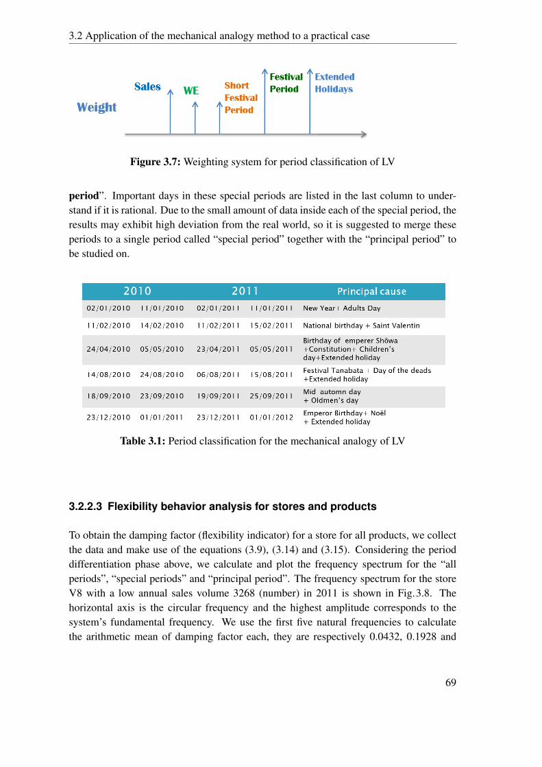
3.2 Application of the mechanical analogy method to a practical case
Figure 3.7: Weighting system for period classification of LV
period”. Important days in these special periods are listed in the last column to under-stand if it is rational. Due to the small amount of data inside each of the special period, theresults may exhibit high deviation from the real world, so it is suggested to merge theseperiods to a single period called “special period” together with the “principal period” tobe studied on.
Table 3.1: Period classification for the mechanical analogy of LV
3.2.2.3 Flexibility behavior analysis for stores and products
To obtain the damping factor (flexibility indicator) for a store for all products, we collectthe data and make use of the equations (3.9), (3.14) and (3.15). Considering the perioddifferentiation phase above, we calculate and plot the frequency spectrum for the “allperiods”, “special periods” and “principal period”. The frequency spectrum for the storeV8 with a low annual sales volume 3268 (number) in 2011 is shown in Fig.3.8. Thehorizontal axis is the circular frequency and the highest amplitude corresponds to thesystem’s fundamental frequency. We use the first five natural frequencies to calculatethe arithmetic mean of damping factor each, they are respectively 0.0432, 0.1928 and
69

Chapter 3 Measurements and methodologies on supply chain flexibility
0.0442 for all periods, special periods and principal periods. The peak of special periodsis explicit.
With these results, it is observed that the flexibility manifested in special periods are sig-nificantly higher than those in all periods and principal period. This is mainly becauseof i): The company anticipates better responsive behavior and may have planned bettermodification of configuration in special periods; ii) The sampling points of special periodsdata are not as enough as the normal periods, therefore, the results may be not represen-tative to compare that of special periods with those of all periods and principal period.However, in case of ii), it remains reasonable to compare the flexibility results of specialperiods with those of other stores, since they are all based on the same period length ofsampling data.
Figure 3.8: Frequency spectrum for store V8 in LV
This is only the results for one store V8 with all products, and it is of great value tocompare flexibility results with those of different stores. The frequency spectrum of storeV36 with a higher annul sales volume 43107 (number) in 2011 is presented by threeperiods in Fig.3.9. Its flexibility damping factors are respectively 0.1147, 0.2495 and0.0999 for all periods, special periods and principal period. Thus, compared with resultsof store V8, the V36 manifest better flexibilities. It is noticeable that sales volume of V36
70

3.2 Application of the mechanical analogy method to a practical case
is greater than V8, implying to a question that, does the stores of bigger volume havebetter flexibility performances in LV? Does the stores of smaller volume provides lowerflexibilities? These are inevitable further questions to answer in this study.
As a result, in order to analyze the flexibility behavior for different stores, we propose toclassify these stores in different groups as “Very Important”, “Important”, “Normal” and“Less Important” according to adequate criteria. Multiple criteria can be used to classifythem:
• Annual sales volume of the store
• Size (surface) and number of employees of the store
• Status of the store (independent store or integrated into large commercial stores)
• ...
Figure 3.9: Frequency spectrum for store V36 in LV
Due to lack of information, we simply propose to classify the stores of LV by the annualsales volume, that is, the category of stores 3, 2, 1, 0 with upgrading sales volume.
71

Chapter 3 Measurements and methodologies on supply chain flexibility
Same to the classification of stores, the product references can should be prudently classi-fied as well. They are supposed to be classified as “Very Important”, “Important”, “Nor-mal” and “Less Important”. Multiple criteria can be used to classify them:
• Annual sales volume of the product
• Net profit compared to sales volume of the product
• The sales stability during the business year of the product
LV has already a rough classification of their products: Seasonal, Slow, NP, Uni-sex,Women, Men and EndLife. But this classification is not really always representative ofthe product nature, for example, certain products in Men are massively sold to women,and the border among Slow, Uni-sex and Men are not clearly defined. In this case, weare agreed to classify them in this study briefly by the ranking of sales volume of eachproduct, as class A, B, C, D, E, F.
With this combined classification of stores and products, we finally obtain a result table ofdamping factor, which indicates the flexibility in each combined category in the followingtable.
Table 3.2: Flexibilities for stores and products in LV
From the Tab.3.2, we can see that the “important product [A]” provides the best flexibilityfor all stores and almost the best compared with all products. Particularly, the “importantproduct [A]” in “important store [0]” manifests a flexibility factor of 0.2417, colored inred, and it is almost the highest value in the table. This may be explained by better oper-ational planning, more adequate strategies of replenishment and more products placed ininventory or in regional warehouses for this category of products and stores. We observethe “important product [A]” manifests better flexibilities in whatever store, whereas the“important store [0]” does not lead to better flexibility for all the products.
72

3.2 Application of the mechanical analogy method to a practical case
The significant tendency is that, for stores in less volume and products in less volume,flexibilities go down gradually along with their sales volumes. Meanwhile, we have ob-served some exceptions for “important store [1]”, the store group with second sales vol-ume, whose flexibilities in “important product [B], [C] and [E]” are a bit higher thanthat in “important product [A]”. This result may be a little strange, but not difficult toexplain. It is very likely that the “important store [0]” has attracted too much attentionof clients for the most demanded product [A], and partakes quite a lot part of pressionsfor store [1]. Consequently, store [1] could provide better flexibilities under less demandpressions. And it must be noted that, the “important product [B]” in “important store [1]exhibits the best flexibility in value 0.2465 among all products and stores.
Another exception occurs for “important product [D]”, classified into [D] claims its unim-portance. Whereas, unimportance + unimportance may not always sum up to unimpor-tance, the product [D] achieves better flexibility (colored in blue) in store [2] and store[3], which are both store groups with quite minor sales volumes. This phenomenon is un-derstandable: while other important stores and important products have stuck into fierceand complex situation, product [D] remains in peace and receives clients in store [2] andstore [3] in tranquility. And it is not the only one, the same happens to product [E] instore [1], colored in orange, with 0.0719 a bit higher than 0.0656 in store [0]. But, un-fortunately, for the last “important product [F]”, no miracle have come to this category:it exhibit bad flexibilities for all stores, and product [F] in store [3] has shown the worstflexibility among all products and stores.
Figure 3.10: Comparison for flexibility curve in principal and special periods
73

Chapter 3 Measurements and methodologies on supply chain flexibility
By comparing flexibility behaviors and the flexibility evolution during two years for dif-ferent stores by volume in Fig.3.10, we observe that a store with bigger annual salesvolume presents relatively higher flexibility. These stores has shown generally less im-portant sensitivity to environmental changes and consequently, become more flexible. Itis clear that for stores with lower annual volume of sales around 20000, its flexibilitycurve turns out to be not quite smooth. These stores are generally more sensitive to ex-ternal excitation (demand) mainly for each group of products. From this curve, we canconclude their flexibilities are generally lower and not as stable as the bigger stores, whichcoincides with the real situation of the company.
The sharp jump near the volume 40000 is an exception, possibly due to an accident orother emergency in the store’s configuration. Moreover, we can see that the evolutionvalue of flexibility in 2010 is generally higher than the year 2011, which implies, eitherthe strategy of the year 2010 is more flexible than the year 2011, either the configurationin stores themselves became more flexible (e.g. new inventory and replenishment poli-cies). Or, if there were a lot more new stores opened in Japan, they may share demandflexibilities and partake demand pressions. In this case, flexibility in each single store maybe not satisfiable temporally, but the overall flexibility of all the Japan division would bebetter in the long term. Normally, the more stores opened, the more buffers (damping)would appear.
74

3.2 Application of the mechanical analogy method to a practical case
3.2.3 A procedure to implement the mechanical analogyevaluation in supply chain
In the previous section, we have exploited the mechanical analogy method to obtain flex-ibility evaluations from the damping factor in stores’ level. The implementation of thismethod in supply chain is not difficult, but a little different from the manufacturing casementioned in sec.3.2.1.3, with a new phase called period-differentiation and more detailedanalysis in our study.
In this part, we try to extend this method to be applied to whole supply chain, and establisha procedure to carry out this flexibility assessment.
Supply Chain is a widely defined notion consists of a set of necessary resources and fa-cilities including manufacturing resources. In Fig.3.6, flexibility assessment using theanalogical method, can take place not only in every single stage but also in multiple ech-elons in distribution. For example, end-customer demand as input, and order of regionalwarehouse from central warehouse as output; or orders from store to regional warehousesas input, and orders from regional warehouse to central warehouse as output. In everyechelon and for multiple echelons, this method is always applicable.
Nevertheless, in the LV application, the “demand” talked about is the end-customer de-mand specified in order quantity. In fact, the “demand” can be also characterized by time,that means, by the order’s real processing time. In the distribution echelon, one can takethe estimated lead time as input data, and the real processing time (delay) of delivered or-ders as output data. In this case, orders are characterized in “time” instead of “quantity”.As a result, researchers must collect input and output data specified in time length. How-ever, this change of data type does not lead to inconveniences, because nowadays, withthe help of Radio Frequency IDentification (RFID) technology, more and more productsare immediately recorded by their step-by-step delivery operations. Consequently, thedata recorded in time is not difficult to acquire. Therefore, on condition that products arerecorded for each stage or for major stages (e.g. in Fig.3.6), the distribution level can alsoadopt the time data to implement the flexibility evaluation.
For manufacturing, Chryssolouris [Chr96] considers a manufacturing system producingaluminum profiles. He adopts the estimated processing times of finished aluminum pro-files as input data, and real flow times of the production as output data (response). Thismanufacturing system consists of different stages of extrusion process, heat treatment,transit buffer, chemical surfaces treatment and packing operations. However, on onehand, Chryssolouris only evaluates the overall flexibility at the stage of finished aluminumprofiles. Flexibility assessment in using the mechanical analogy, can take place in vari-ous echelons of distribution and also in different stages of manufacturing. The analogymethod is applicable to any single intermediate stage and multiple stages of the manu-facturing system. For example, one can take the estimated processing time of combined
75
Chapter 3 Measurements and methodologies on supply chain flexibility
“heat treatment - transit - chemical surfaces treatment” as input, and real flow time of thecombined “heat treatment - transit - chemical surfaces treatment” as output. On the otherhand, it is noticed that input and output data in this case are only time data. If times canbe recorded, their production quantities should be easily derived as well, and probably,already recorded with their times at the same time. Thus, in the analogy evaluation ofmanufacturing flexibility, the input and output data can be both specified in manufactur-ing quantities as well. That means the inverse direction of data type “quantity” to data“time” is possible as well as in manufacturing echelon.
Other than manufacturing and distribution activities, the supply echelon has not been cov-ered by any existed flexibility study with analogy method. However, its evaluation couldbe conducted in the same way. In manufacturing sites, the accomplishment rate of pro-duction orders counts well for production planning; whereas in distribution echelon, thedelivery service level for clients anounces its performance. And in supply echelon, servicelevels provided by suppliers vs industrial clients (e.g. manufacturer, assembler, compo-nents manufacturer...) in terms of time, quantity and cost, counts well for the selectionof suppliers. Furthermore, different suppliers may co-exist to offer various raw materialsand semi-finished articles in a multiple-stage structure. Thus, this analogy method is stillapplicable to supply echelon: one can compare the flexibilities among different articlesoffered by only one supplier, and among several suppliers providing the same article. Inthe same way, the results of analogical flexibility assessment would be understandable forsuppliers, and can be conducted in every single stage and multiple stages of the supplyechelon. In addition, “time” and “quantity” remain as two regular data types for inputand output data in order to evaluate the flexibility in supply echelon.
To extend this method to each stage of supply chain, we propose to define a new term:finished rate. This finished rate aim at being the notion of “service level for clients” indistribution echelon, the notion of “fulfillment of production orders” in manufacturingechelon, and the notion of “satisfactory rate of industrial clients to their suppliers” insupply echelon.
Generally, it describes the accomplishment situation of any orders in any stage of supplychain (supply / production / distribution) in terms of time and quantity. That means, itdepicts the order accomplishment regardless of different supply chain echelons. Thisis an important term, indicating whether it is appropriate to exploit mechanical analogymethod to evaluate the flexibility performance of the studied problem. It is detailed in thefollowing paragraphs.
In conclusion, we consider the mechanical analogy method appropriate to be exploitedregardless of various supply chain echelons (supply / manufacturing / distribution / orsmall stages among them).
Before carrying out the evaluation, a lot of preparation works need to be done. The fin-
76

3.2 Application of the mechanical analogy method to a practical case
ished rate is only one data provided from industrial world. For this, we propose to outlineand establish a complete evaluation procedure, which would be useful for all further workto be applied in supply chain:
(I) Appropriateness checking
The initial phase to identify whether the studied system is appropriate to be assimilated toa vibration mechanism and evaluated by the analogy method. This checking phase goesin three steps:
• Study the supply chain situation of the company;
• Check the finished rate and make sure if there exist relatively drastic increases ininput data within quite a short period;
• Check whether the finished rate reaches 100%;
If there exist too many drastic changes leading to a very low service level, it may be ofno value to make use of analogy method for the studied problem. The reason is that theanalogical response of corresponding vibration system, may frequently jump out of reachand lead to distorted, meaningless results. Here “the studied problem” can be either fora whole supply chain, or in one echelon, one small stage and for several multiple stagesof supply chain. In the following paragraphs we just use “the studied supply chain” forshort.
If the finished rate of the studied supply chain achieves or closely approaches 100%,the analogical mechanical system is probably over damped, so that the correspondingfrequency spectrum of the mechanical vibration system could not arrive at any meaningfulresults.
Fortunately, these two situations are rarely seen in most part of industrial world. Gener-ally, firms in the market may exhibit a good finished rate but still can be improved.
(II) Data preparation
The preparation phase to carry out the mechanical analogy method for the studied prob-lem. It is followed in three steps:
• Identify the input data: type of data (time/quantity), physical meaning with analogyto excitation force of mechanical system;
• Identify the output data: type of data (time/quantity), physical meaning with anal-ogy to vibration response of mechanical system;
• Prepare the required input and output data;
77

Chapter 3 Measurements and methodologies on supply chain flexibility
The data required in analogy method is not difficult to gather from the industrial world,as explained in sec.3.2.1.3.
However, it is of great importance that input and output data must be understandable andpassable for its appropriate physical meaning in supply chain. For example, in the previ-ous LV application, the input is considered to be “sales quantity in LV stores per productreference per store per day”, the output as “delivery product quantity from regional ware-houses to stores per product per store per day”. This input and output can not be changedto the inverted sense, because stores of LV do work mainly in a order-driven mode, thatmeans products are first sold and demanded in stores, and secondly, stores place com-mands in regional warehouses to receive sufficient replenishment. Thus, the input data is“sales in LV stores”, serves as the analogical excitation to system, which coincides withthe physical meaning in the studied supply chain.
(III) Period classification
The second preparation phase in order to carry out the mechanical analogy method for thestudied problem, is concerned with period issues:
• Prepare all the data in all working/opening periods of the studied supply chain;
• Check if the company retains the same internal configurations among different pe-riods during a business year;
• Check if the input data shows the same pattern during a year;
• Classify heterogeneous periods;
The opening periods of a company differ from supply department, manufacturing depart-ment and distribution department. For example, for a great part of holidays (e.g. Saturday)some manufacturing sites and warehouse centers do not continue to work, whilst storesin distribution echelon may keep open for clients. Therefore, the period information mustbe provided by distinguished input and output periods.
Moreover, in industrial world, a company intends to plan various promotions in periodsto pre-stock for future occasions and to recruit temporary employees. As a result, theinternal configuration in a company could not remain the same. So does the input data,which is rarely distributed in the same pattern over a year. And, if the company does notmaintain regular activities during holidays, the results will be more different.
In this way, we suggest the researcher to lance an appropriate and complete period-classification table before flexibility evaluation, not only in use of analogical method,but also for other methods, because all changes of internal configuration will impact onflexibility evaluation methods and lead to different flexibility behaviors. The researcheris recommended to list and highlight all the unusual periods with time length by internal
78

3.2 Application of the mechanical analogy method to a practical case
configuration changes, and also by different input data patterns, as what we have con-structed by a weighting system in Fig.3.7 and Tab.3.1.
(IV) Object classification
Before the data computation and consecutive analysis, researcher is suggested to identifythe studied objects by different criterion on which he intends to study and analyze, inorder to assess the right flexibility, and make meaningful comparisons.
• Identify the studied objects;
• Group the studied objects by different criterion;
In the LV case, flexibility assessment is carried out for two study objects: stores and prod-ucts. Stores can be concreted and distinguished as smaller groups by its sales volume, size,number of employees, independent status, etc., while products need to be classified andgrouped by multiple criteria, such as sales volume, net profit, sex aimed by the product,sales stability, etc.
In order to conduct understandable results for industrial use, the classification of the stud-ied objects by groups in appropriate criteria is of great value. With this classification, flex-ibility evaluation could be carried out by different groups of input and output data, leadingto any indications relating to their intrinsic properties, which may be further linked withinternal configurations in the company.
(V) Data computation
• Calculate the analogical damping factor;
• Analyze flexibility behaviors by object groups.
Data computation is the last and core phase of the mechanical analogy procedure.
Input data and output data of the studied supply chain are receptively entered to algorithm,waiting to be transformed to Transfer Function in the frequency domain. Afterwards,response of vibration system in the frequency spectrum are recorded, and damping factorsreflecting system’s flexibility are derived.
In adopting this procedure, the researcher can easily arrive at a comprehensive assessmenton flexibility on studied objects by groups in periods, and draw conclusions by objectcharacteristics. It is claimed that flexibility behavior is closely related to object propertyand company’s internal configuration, thus, if the object properties of the studied problemare explicitly known, all flexibility behaviors can be consequently well reasoned. And ifcompany operations to change the internal configuration in the past are known as well,
79

Chapter 3 Measurements and methodologies on supply chain flexibility
various flexibility behaviors can be directly linked to its operations, and thus fully rea-soned. Therefore, it is a good method to identify consequent flexibilities according todifferent strategic operations.
80

3.3 Conclusion
3.3 Conclusion
This chapter addresses supply chain flexibility from a quantitative point of view. We firstreview the existing evaluation methodologies on supply chain flexibility, and confirm thatquantitative studies are now booming but still quite limited.
In order to clarify the methodology to integrate some precised flexibility dimensions, wehave presented the method of Rogalski [Rog11] , which incorporates volume flexibility,product-mix flexibility and expansion flexibility respectively into the model, and can beexpressed separately without interfering too much in details. Other measures and methodsas Penalty of Change, Design of Systems for Manufacture, Mechanical Analogy, Simu-lation based on Petra nets, Toolbox Approach and methodologies involving flexibilityconsiderations are reviewed.
Among these different methodologies, we consider Mechanical Analogy method quiteuseful and practical to evaluate the flexibility performance in supply chain. It does notrequire numerous data in detail or hard to collect, and is interested and appreciated byour industrial partners. As the method was rough and has never been applied to supplychain level, we start off to investigate its feature, assess its advantages and drawbacks, andestablish a complete procedure to implement this method in supply chain. We discoverthat the period classification is inevitable because the system may take reconfigurationsin different periods.
By exploiting this method, we conduct a case study in Louis Vuitton to evaluate the flex-ibility for stores and products in Japan. The results lead to the conclusion that flexibilityof a small store is generally lower, and not as stable as the bigger stores during a year,whereas the products in bigger volume exhibit a general better flexibility throughout thewhole year. These results coincide with the real situation of the firm. As a result, a generalevaluation procedure to carry out this method in supply chain is detailed in this chapter.
Although the mechanical analogy concept could be exploited to calculate correspondingdamping factor, in order to assess the flexibility of a supply chain system (a supply chainor part of supply chain), the detailed logic on how the analogy concept impacts the mod-eling of supply chain remains unclear. As described in sec.3.2.1, a simple mechanicalvibration system of a single degree of freedom, consists of a mass m, an elastic spring kand a damper c, including three main intrinsic attributes of a mechanical system: its iner-tia, damping and stiffness. It is of little difficulty to draw damping factor as the flexibilitymeasure, but the attributes of inertia and stiffness are also important keys to understandthe supply chain’s behavior. We can see that the mass m of system could be calculatedfrom 3.12, which make it possible to be deduced from the flexibility, but the relation ofstiffness k and damping c is still hard to derive. This is a good research subject to beinvestigated in future researches.
81


4 Integrated production andtransportation planning withgiven flexibility
Industrial planning problems arise in different circumstances, so does incorporated flex-ibilites. Planning problems are frequently encountered in each echelon of supply chainand influence directly or indirectly facilities’ performance, while flexibility issues mayoccur in each stage of supply chain. It is known that two primary goals in both produc-tion and transportation planning are to satisfy the customer demands and to bring in thelowest cost. However, the problems synchronizing the production plan and the transporta-tion plan with some detailed flexibility issues, have received little attention in the priorliterature and applications in practice.
In this chapter we concentrate on how to exploit and to manager the flexibility in industrialplanning problems. We propose to solve an integrated production and transportation plan-ning problems with given flexibility considerations, with data provided by the water com-pany Evian. To start off, we first present a short introduction to production planning andtransportation planning literature respectively. Afterwards, literature on synchronized orintegrated production and transportation planning problems is comprehensively reviewedin sec.4.2, as a contribution of literature. In the following, we present an entire case studyfor the French mineral water company in sec.4.3, with special consideration on givenflexibilities. This integrated problem has been developed and solved in two cost-basedcombinatorial optimization models which are slightly different and respectively describedin sec.4.4 and sec.4.5. The next sec.4.6 concludes this part of thesis.
83
Chapter 4 Integrated production and transportation planning with given flexibility
4.1 Introduction to industrial production andtransportation planning problems
4.1.1 Production planning
To appropriately make use of limited resources in order to meet industrial goals, manufac-turers have to make decisions on allocating resources and scheduling their activities overa planning horizon. Production and scheduling planning in a supply chain is viewed as theplanning of the acquisition of different production resources and raw materials, as wellas the planning of the production activities of staff to the ability to release accurate de-livery times for the customer. It prepares a detailed plan in production process to achieveproduction goals economically.
Generally, production planning provides answers to three following major questions:
• What work should be done?
• How much time will be taken to perform the work?
• Which resources (site, machine, labor, ...) are needed to carry out the work?
Thus, solutions of production planning will decide the ways and means of productionactivities that affect several organizational echelons mainly grouped into three broad cat-egories:
• Strategic level, involving capital investment, policy formulation, and location de-sign of physical facilities in a long term
• Tactical level, dealing primarily with aggregate production planning in mediumterm
• Operational level, concerning detailed production scheduling issues in short timehorizon
The three categories of production decisions differ largely in terms of level of manage-ment responsibility and its interaction, length of the planning horizon needed to assesstheir consequences, level of the required information and also the degree of uncertaintiesinherent in each decision.
An ideal hierarchical production structure is illustrated in Fig.4.1, where the system op-erates and allocates resources and client orders in a centralized manner, separates severaldistinct planning areas defined into organizational units and coordinates them with a fewcontrolled interfaces. It utilizes the natural time-structure of the planning process and re-quires the aggregation of data. Thus, a perfect hierarchical structure conveys productiondecisions fluently by decision level, decreases incidents and chaos in sub-problems and
84

4.1 Introduction to industrial production and transportation planning problems
enables most important problems to be visible and traceable. However, an ideal hierarchi-cal production planning is difficult to achieve due to enormous work on data aggregationand cooperation among departments, especially if the company did not design and imple-ment such a framework in the first place.
Figure 4.1: Hierarchical production structure
This structure interests the partners in our Chair Supply Chain. The steel tube produc-tion company Vallourec takes on a central planning department to allocate client ordersto production sites, with some special quotas reserved for several sites, which is already atypical centralized and almost hierarchical production planning system. Furthermore, thecompany has tried to reorganize its existent distinct and disperse production planning pro-cess in different sites in order to convert into an ideal hierarchical structure. The companyinclined to implement an uniform planning tool (APS - advanced planning and schedul-ing system) across the planning structure, but was confronted with the situation whereeach site utilizes its own tool or methods. Due to enormous information and complicatedcooperation among departments, especially because the sites have accustomed to theirown planning process from the beginning, the perfection and standardization of its hier-archical organization leads to a pretty high cost which would be not at all worthy. In thiscontext, the company has finally abandoned its project on APS to reform and standardizeits production structure.
In academic field, a lot of investigations have been done on production planning problems.When focusing on tactical and operational production plannings, we could say first studiesin this field started with constant demand, continuous time and infinite horizon. If thereis no obvious capacity constraints, the classical economic order quantity model is usefulfor a single-level production process [Har13, Wil34]. Furthermore, models with dynamicdemand, discrete time and finite horizon, are generally referred to as dynamic lot sizing,seeking a minimum cost plan that meets all constraints over a finite horizon, which isoften formulated into mixed integer programs (MIP).
85
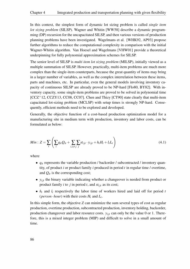
Chapter 4 Integrated production and transportation planning with given flexibility
In this context, the simplest form of dynamic lot sizing problem is called single itemlot sizing problem (SILSP). Wagner and Whitin [WW58] describe a dynamic program-ming (DP) recursion for the uncapacitated SILSP, and then various versions of productionplanning problems have been investigated. Wagelmans et al. [WHK92, AP93] proposefurther algorithms to reduce the computational complexity in comparison with the initialWagner-Whitin algorithm. Van Hoesel and Wagelmans [VHW01] provide a theoreticalunderpinning for fully polynomial approximation schemes for SILSP.
The senior level of SILSP is multi item lot sizing problem (MILSP), initially viewed as amultiple summation of SILSP. However, practically, multi-item problems are much morecomplex than the single-item counterparts, because the great quantity of items may bringin a larger number of variables, as well as the complex interrelation between these items,parts and machines, etc. In particular, even the general models involving inventory ca-pacity of continuous SILSP are already proved to be NP-hard [Flo80, BY82]. With in-ventory capacity, some single-item problems are proved to be solved in polynomial time[CCZ+12, CCZY13, CC08, CC07]. Chen and Thizy [CT90] state clearly that multi-itemcapacitated lot-sizing problem (MCLSP) with setup times is strongly NP-hard. Conse-quently, efficient methods need to be explored and developed.
Generally, the objective function of a cost-based production optimization model for amanufacturing site in medium term with production, inventory and labor costs, can beformulated as below:
Min : Z = ∑t
(∑
iqitQit + ∑
i,i 6= j∑
jsti jt · yi jt +htHt + ltLt
)(4.1)
where
• qit represents the variable production / backorder / subcontracted / inventory quan-tity, of product i or product family i produced in period t in regular time / overtime,and Qit is the corresponding cost;
• yi jt the binary variable indicating whether a changeover is needed from product orproduct family i to j in period t, and sti jt as its cost;
• ht and lt respectively the labor time of workers hired and laid off for period t(person ·hour) with their costs Ht and Lt .
In this simple form, the objective Z can minimize the sum several types of cost as regularproduction, overtime production, subcontracted production, inventory holding, backorder,production changeover and labor resource costs. yi jt can only be the value 0 or 1. There-fore, this is a mixed integer problem (MIP) and difficult to solve in a small amount oftime.
86

4.1 Introduction to industrial production and transportation planning problems
In order to solve the MIP problems efficiently, a variety of approaches have been investi-gated, from exact mathematical programming methods to heuristic approaches. Many ex-act mathematical methods attempt to strengthen the original formulation by adding validinequalities [BVRW84, PW94] and by extending model reformulations [EM87, Wol02].
Since real-world problems are computationally difficult, different heuristic methods areproposed to tackle them. Among the different heuristics in the literature, we can generallyclassify them into simple heuristics and iterative ones. The simple heuristics are usuallyone-pass “constructive” (greedy) heuristics, which starts with no solution and tries toconstruct one in a step-by-step manner. The other iterative heuristics are usually so called“improvement” heuristics, starting with a feasible solution and trying to improve the cur-rent one in an iterative manner. This type of heuristics has been carried out mainly in twocategories: meta-heuristics such as Genetic Algorithms [HK96], Tabu Search [GDS01]and Simulated Annealing [SKW93]; relaxation techniques that relax capacity constraintsto decompose the initial problem into single-item uncapacitated subproblems.
Furthermore, problem-specific heuristics are proposed to solve individual problems. Maesand Wassenhove [MW88] provide an early review on problem-specific heuristics. FurtherLagrangian-based decomposition is also developed [TD96] and Local Search method isfrequently mentioned [SE05]. Among these heuristics, Tian et al. [TWK11] suggest aniterative approach to jointly optimize the tactical safety stock level and production plan-ning. Apart from various problem-specific heuristics, the generalized MIP heuristics arecomparatively few. Pochet and Wolsey [PW06] provide a general review of MIP heuris-tics, such as LP-and-fix and relax-and-fix. Allaoui and Artiba [AA06, AA14] study ahybrid flow shop scheduling with machines that are not always available due to stochasticbreakdowns and preventive maintenance. They propose dynamic programming to solvetwo-machine flow shop, a branch and bound algorithm to solve the two-stage hybrid flowshop, and three heuristics for the worst-case performances.
In addition, for some models involving multiple objectives, one can associate a weightwith each of these objectives to merge them into a single objective function. Differentapproaches are explored for multi-objective models with different working assumptions,such as, artificial neural network [McM01, GFG06, SV09], fuzzy simulation [MM08,JS09], genetic algorithm [CH05, SV09], problem-specific and random search heuristics[KNK12], etc.
4.1.2 Transportation planning
Transportation planning plays a linkage between each two steps of supply chain, taking alltransport functions and sub-functions into a system of commodities movement. Compa-nies are traditionally involved in different steps [FW81] such as production/manufacturing
87

Chapter 4 Integrated production and transportation planning with given flexibility
plants, storage, warehousing services, merchandising establishments, transportation, whole-saling, and retail sale. According to the 23rd annual CSCMP States of Logistics Reportpresented by Wilson [Wil12], transportation costs in 2011 in the USA represented 64%of the total logistics costs, inventory costs 33% and administrative costs 4%. Around onethird to two thirds of the expenses of enterprises’ logistics costs are spent on transporta-tion, playing a vital role in the determination of product price.
Besides, costs of transportation vary from different industrial sectors [TYT+05]: for thoseproducts with small volume, low weight and high value, transportation cost accounts foronly a tiny part of sale and is less regarded; for those products with big volume, heavyweight and mainly low unit value, transportation occupies a very big part of sale andaffects profits more, and therefore it is more regarded.
The transportation problems discussed here mainly refer to distribution problems in asupply chain. On the downstream side of supply chain, distribution activity consists oftransfer movements of multiple commodities from plants to demand markets directly orindirectly, the latter concerned with intermediate transshipment via some additional fa-cilities such as warehouses or distribution centers (DC). Usually, storage volume may beplanned for high value commodities whose market demand is difficult to forecast, whilethe other fast-moving items may be hold in inventory at the DCs to achieve a better re-sponsiveness. These intermediate locations between plants and final customers facilitatethe consolidation of shipments from different supply plants to meet the demand marketthrough accumulated product inventories, in order to achieve lower transportation costsin a shorter response time. Two further tasks are usually performed at distribution centersand warehouses, namely consolidation and split (break-bulk) operations. Consolidationconsists of combining shipments of similar or different delivery from several origins,while split goes the opposite side through which a large load from a given source is splitinto several smaller deliveries [TOG01].
The transportation problems also differ one from another according to decision level andplanning horizon, and can be further classified in to strategic, tactical, operational prob-lems in the literature. With increasing intermediate components added into the down-stream side of supply chain, the transportation system is quickly extended to N-echelonnetwork (N ≥ 2) and the 2-echelon case is mostly studied. The N-echelon location routingproblem and the inventory routing problem are the two well-known tactical distributionproblems. In the operational planning phase, vehicle routes and schedules are periodicallygenerated based on available resources, supplier and customer locations and product de-mands. Research attention have been mainly attracted on strategic and tactical planning,and most operational optimization approaches for N-echelon transportation system areextensions of methods for the classical vehicle routing problem. Economical savings byusing N-echelon transportation network are also partly due to different sizes of vehiclesat different levels. Haul trucks are assigned to move end products from factories to in-
88

4.1 Introduction to industrial production and transportation planning problems
termediate facilities and vehicles with lower capacity transfer loads between intermediatefacilities and the final destinations. Distinct modes of transportation may vary from truck,air, rail, ships in the water, pipeline and the intermodal manner which combines varioustransportation modes in different steps.
Geoffrion and Graves [GG74] are the first to study the two-stage version of multi-commoditytransportation problem, considering a multi-plant, multi-commodity, multi-DC structure.This is a MILP problem using Bender Decomposition procedure to get LP subproblems.To understand the N-echelon transportation problem, we could illustrate below a simple2-echelon transportation routing network by a graph G(I, A) in Fig.4.2. Generally, inthe node set I at least three types of nodes are considered: (i) source nodes IS, such asmanufacturing storage sites where vehicles only pick up finises items; (ii) intermediatenodes IM, like regional warehouses or distribution centers where vehicles turn to carryout pickup or delivery operations; (iii) destination nodes ID, such as consumer locationswhere vehicles come to accomplish their deliveries. In the arc set A, every arc (i, j) ∈ Abetween the nodes is characterized by a distance-based or a time-based transportationcost ci j and a journey time ti j served by some vehicles Vi. It is assumed that the triangleinequality must be satisfied that ci j + c jk > cik, where (i, j, k) ∈ I.
Figure 4.2: A two-echelon distribution network
Transportation operation is costly. It is frequently studied by two parts: fixed cost andvariable cost. A basic assumption asserts that transportation cost is directly proportional
89
Chapter 4 Integrated production and transportation planning with given flexibility
to the number of product units transported [Dia91], thus, some studies consider a purelyproportional quantity dependent distribution cost. Apart from this assumption, many prac-tical transportation and distribution problems can be modeled as a fixed charge transporta-tion problem [AK99, EEP06, AKVL07], in which there exist two kinds of cost: (i) a con-tinuous variable cost that linearly increases with the quantity transported between a sourceand a destination, and (ii) a fixed charge, which may represent a cost of renting a railwaytrain, landing fee at an airport or toll charges on a high way, incurs if a nonzero quan-tity is transported between a source and a destination. Hirsch and Dantzig [HD54] areamong the first to explain and formulate the fixed charge transportation problem (FCTP),and Balinski [Bal61] proposes a heuristic method to solve this type of problem. A broadbody of literature has started on this category and proposed solution techniques to solvethe one-echelon FCTP [PKZ90, AADRR09], which is NP-hard if we solve it with ex-act algorithm [SAMD98]. Sun et al. [SAMD98] and Gen and Cheng [GC00] proposeusing metaheuristics such as tabu-search or genetic algorithms to solve the fixed chargetransportation problem.
While solving the problem in exact algorithm is comparatively hard, the mathematicalmodel construction is not complicated. A simple form of multi-plant, multi-commodity,multi-DC, multi-customer and two-echelon transportation problem at tactical level can beeasily formulated together with a set of mutual constraints, see Annex I for details.
Researchers have attempted to solve multi-echelon transportation problems using exactalgorithms and heuristics (e.g. [PJ98, THR00]). Syarif and Gen [SG03] describe a dou-ble spanning tree-based hybrid genetic algorithm with a chromosome for each echelonrepresented by Prüfer numbers. In combinatorial mathematics, the Prüfer numbers (alsoPrüfer code or Prüfer sequence) of a labeled tree is a unique sequence associated withthe tree, which has length n−2 for a tree of n vertices and can be generated by a simpleiterative algorithm [Prü18]. When taking the opening cost of a DC into consideration,Gen et al. [GAL06] propose a genetic algorithm using a priority-based encoding pro-cedure to solve the two-stage transportation problem, with limited number of openedDCs. Such two-stage transportation problems are NP-hard [GAL06]. Jawahar and Balaji[JB09] present a genetic algorithm considering a chromosome to represent a candidatesolution from DCs to customers and the other part of solution by applying the Least CostMethod (LCM), which makes use of a cost called equivalent cost, per-unit transportationcost and the fixed cost associated with a route. Later, Balaji and Jawahar [BJ10] developa simulated annealing algorithm to solve the same problem, compared with the solutionobtained by a LP using an approximate per-unit transportation cost, they provide a bettersolution. Antony Arokia Durai Raj and Rajendran [AADRR12] provide genetic algo-rithms to solve a two-echelon transportation problem with two different scenarios, wherethe first is similar to that of [GAL06] and the second considers the opening cost of a DCsimilar to [JB09]. They also present a methodology to represent the two-echelon trans-
90
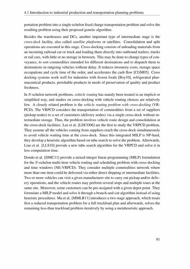
4.1 Introduction to industrial production and transportation planning problems
portation problem into a single-echelon fixed charge transportation problem and solve theresulting problem using their proposed genetic algorithm.
Besides the warehouses and DCs, another important type of intermediate stage is thecross-dock facility, also called satellite platforms or satellites. Consolidation and splitoperations are executed in this stage. Cross-docking consists of unloading materials froman incoming railroad car or truck and loading them directly into outbound trailers, trucksor rail cars, with little or no storage in between. This may be done to change types of con-veyance, to sort commodities intended for different destinations and to dispatch them todestinations in outgoing vehicles without delay. It reduces inventory costs, storage spaceoccupations and cycle time of the order, and accelerates the cash flow [CGM05]. Crossdocking systems work well for industries with frozen foods [Boy10], refrigerated phar-maceutical products, perishable products in needs of preservation of quality and productfreshness.
In N-echelon network problems, vehicle routing has mainly been treated in an implicit orsimplified way, and studies on cross-docking with vehicle routing choices are relativelyfew. A closely related problem is the vehicle routing problem with cross-docking (VR-PCD). The VRPCD considers the transportation of commodities from a set of suppliers(pickup nodes) to a set of customers (delivery nodes) via a single cross-dock without in-termediate storage. Thus, the problem involves vehicle route design and consolidation atthe cross-dock facilities. Lee et al. [LDCO06] are the first to study the VRPCD problem.They assume all the vehicles coming from suppliers reach the cross-dock simultaneouslyto avoid vehicle waiting time at the cross-dock. Since this integrated MILP is NP-hard,they develop a heuristic algorithm based on tabu search to solve the problem. Afterwards,Liao et al. [LLS10] provide a new tabu search algorithm for the VRPCD and solve it inless computation time.
Dondo et al. [DMC11] provide a mixed-integer linear programming (MILP) formulationfor the N-echelon multi-item vehicle routing and scheduling problem with cross-dockingand time windows (NE-VRPCD). They consider multiple commodities network wheremore than one item could be delivered via either direct shipping or intermediate facilities.Two or more vehicles can visit a given manufacturer site to carry out pickup and/or deliv-ery operations, and the vehicle routes may perform several stops and multiple tours at thesame site. Moreover, some customers can be pre-assigned with a given depot point. Theyformulate a MILP model and solve it through a branch-and-cut algorithm instead of usingheuristic procedures. Ma et al. [MMLR11] introduces a two-stage approach, which treatsfirst a reduced transportation problem for a full truckload plan and afterwards, solves theremaining less-than truckload problem iteratively by using a metaheuristic approach.
91

Chapter 4 Integrated production and transportation planning with given flexibility
4.2 Review of integrated production andtransportation problems
4.2.1 Introduction of integrated production and transportationproblems
A typical supply chain starts from raw material input flow, followed by correspondingproduction to make finished items and deliveries to different distribution centers untilreaching final customers. The cost of a product come up not only from factory resourcesto convert raw materials to end products but also from resources to deliver the productto customers, make corresponding sales, configure the inventory holding and services tocustomers. The composition of these operational term in total costs varies largely by in-dustry, while the production cost is proved to be the largest part of all costs in almost allthe industries [Che97]. Production and transportation operations can be easily decoupledif a sufficient amount of inventory is permitted between them. Many companies managethe two functions independently with little or no coordination without further consider-ation, which may lead to higher holding costs and longer lead times through the wholesupply chain. The two activities are usually studied separately not only in the industrialfield, but also in academic researches, mainly for reasons: a) each problem itself is al-ready difficult to solve, therefore the combined problem seems intractable and b) differentdepartments in an organization deal with each activity [EEP06].
On one hand, firms in the last decades have recognized that there would be a greater op-portunity to manage supply chain in a coordinated manner than in improving individualfunction areas separately to save the cost. Nevertheless, reduced inventory may resultin closer linkages between production and distribution functions. Production and distri-bution operations have often been considered as two separate operational functions in asupply chain. To achieve optimal operational performance in a supply chain, it is there-fore suggested to integrate these two functions and plan them jointly in a synchronizedway.
On the other hand, a synchronized production and transportation plan is one of funda-mental needs to firms who provide mainly make-to-order products to the market or man-ufacture some kind of time-sensitive products (perishable and seasonal goods, etc.). Asthe number of companies continues to increase in changing themselves to make-to-orderbusiness models, such as assemble-to-order, build-to-order, design-to-order, direct-sell e-business models, the products become customer-made or must be delivered to customerswithin a very short lead time. In some practical cases, products should even be deliv-ered directly from the factory site without any intermediate location transfer. A no-waitsituation occurs in many real working environments, mainly because of limited storage ca-
92
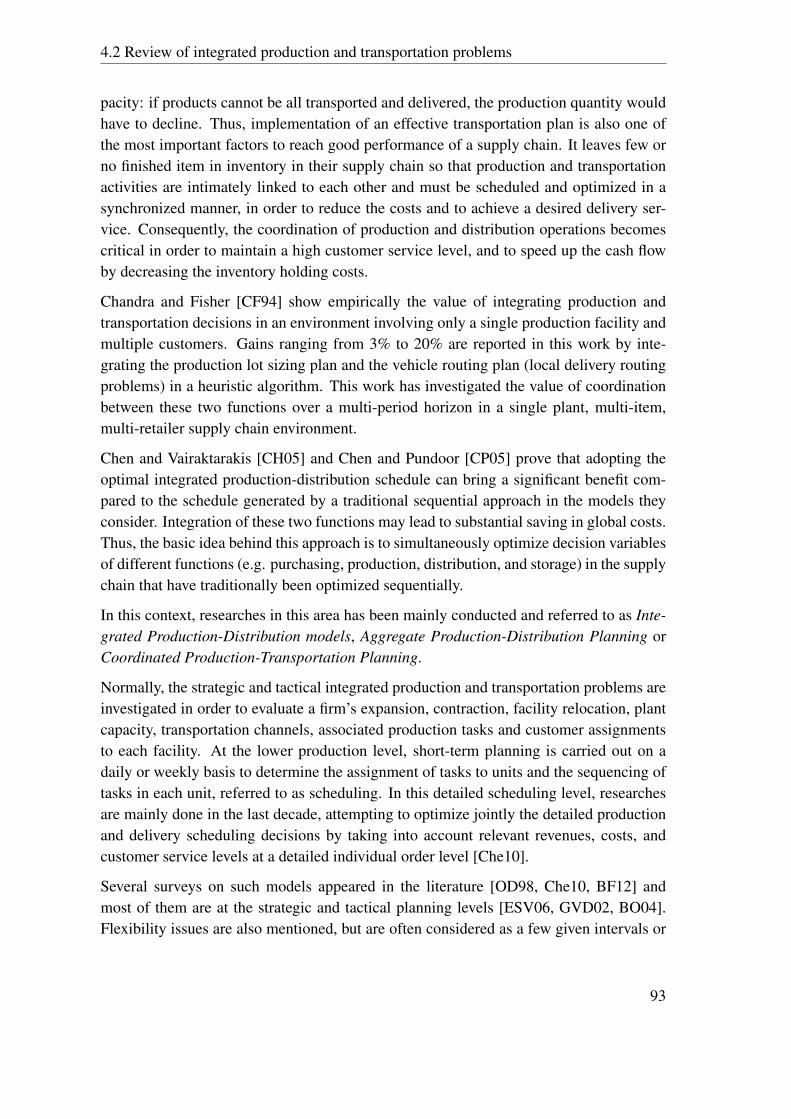
4.2 Review of integrated production and transportation problems
pacity: if products cannot be all transported and delivered, the production quantity wouldhave to decline. Thus, implementation of an effective transportation plan is also one ofthe most important factors to reach good performance of a supply chain. It leaves few orno finished item in inventory in their supply chain so that production and transportationactivities are intimately linked to each other and must be scheduled and optimized in asynchronized manner, in order to reduce the costs and to achieve a desired delivery ser-vice. Consequently, the coordination of production and distribution operations becomescritical in order to maintain a high customer service level, and to speed up the cash flowby decreasing the inventory holding costs.
Chandra and Fisher [CF94] show empirically the value of integrating production andtransportation decisions in an environment involving only a single production facility andmultiple customers. Gains ranging from 3% to 20% are reported in this work by inte-grating the production lot sizing plan and the vehicle routing plan (local delivery routingproblems) in a heuristic algorithm. This work has investigated the value of coordinationbetween these two functions over a multi-period horizon in a single plant, multi-item,multi-retailer supply chain environment.
Chen and Vairaktarakis [CH05] and Chen and Pundoor [CP05] prove that adopting theoptimal integrated production-distribution schedule can bring a significant benefit com-pared to the schedule generated by a traditional sequential approach in the models theyconsider. Integration of these two functions may lead to substantial saving in global costs.Thus, the basic idea behind this approach is to simultaneously optimize decision variablesof different functions (e.g. purchasing, production, distribution, and storage) in the supplychain that have traditionally been optimized sequentially.
In this context, researches in this area has been mainly conducted and referred to as Inte-grated Production-Distribution models, Aggregate Production-Distribution Planning orCoordinated Production-Transportation Planning.
Normally, the strategic and tactical integrated production and transportation problems areinvestigated in order to evaluate a firm’s expansion, contraction, facility relocation, plantcapacity, transportation channels, associated production tasks and customer assignmentsto each facility. At the lower production level, short-term planning is carried out on adaily or weekly basis to determine the assignment of tasks to units and the sequencing oftasks in each unit, referred to as scheduling. In this detailed scheduling level, researchesare mainly done in the last decade, attempting to optimize jointly the detailed productionand delivery scheduling decisions by taking into account relevant revenues, costs, andcustomer service levels at a detailed individual order level [Che10].
Several surveys on such models appeared in the literature [OD98, Che10, BF12] andmost of them are at the strategic and tactical planning levels [ESV06, GVD02, BO04].Flexibility issues are also mentioned, but are often considered as a few given intervals or
93

Chapter 4 Integrated production and transportation planning with given flexibility
fuzzy constraints in the model construction.
4.2.2 General classification of integrated production andtransportation planning problems
Consider a supply chain structure in multiple levels illustrated in Fig.4.3, where the inputsto various manufacturing plants consisting of raw materials can be sourced from a set ofsuppliers, and the output of finished items can be transported to different warehouses anddistribution centers and then to different outlets or to final customers. In this structure,production facilities can be multi-leveled, and so do distribution ones. For a production-transportation problem in a supply chain, the integrated problem can occur at each linkageand each micro or macro bloc in this chain structure.
Figure 4.3: Multi-facility supply chain structure
A macro block problem in the structure Fig.4.3 is often referred to as a production-transportation, facility location-allocation problem. A great deal of study has been carriedout to develop models and exact algorithms in this area, see [RL96, RE05] for a review.Here the term “facility” is expressed in its broadest sense, including entities such as fac-tories, distribution centers, warehouses, retail outlets, computer terminals, schools, hos-pitals, day-care centers, etc. If each facility is limited to a certain capacity, the problem isthen referred to as capacitated facility location problem. The single-source, capacitated fa-cility location problem is the simplest form and is a special case of the capacitated facilitylocation problem in which each customer can only be supplied from exactly one facility.The further extension of the location problem leads to multi-level or multi-echelon facilitylocation problem. These are mainly strategic and tactical decisions: the former indicatingfacility location, capacity and network structure; the latter focusing on how much to shipin a time period, how much inventory to keep, how long a production/distribution cycleshould be, etc.
94

4.2 Review of integrated production and transportation problems
A micro block problem in the structure Fig.4.3 is related to explicit production-distributionproblems in operational level, involving detailed scheduling level decisions such as: whenand on which machine to process a job, when and by which vehicle to deliver a product,what the vehicle routing should be, etc. We can then classify the integrated productionand transportation problems into three main categories:
• (A) Cross-facility, production-transportation, facility location-allocation problemsacross multiple stages of the supply chain
• (B) Explicit scheduling level, production-supplier problems integrating the inboundtransportation and production
• (C) Explicit scheduling level, production-distribution problems integrating the out-bound transportation and production
The problem class (A) and (C) are reviewed successively in the next sections.
The integrated production and inbound problems (B) are often aggregated as a materialcontrol subproblem in problems (A) and thus will not be widely reviewed in this work.We just make a short introduction for problems of class (B) here: an integrated productionand inbound problem (B) treats problems of production and delivery of raw material fromsuppliers. A manufacturer purchases raw material from some suppliers, uses the rawmaterial to manufacture finished products and ships them to customers. Thus, a (B) classproblem contain mainly four components: (i) distribution cost for delivering raw materialfrom the supplier to manufacturer plants; (ii) inventory cost for holding raw materialat manufacturer side; (iii) production cost at manufacturer side; (iv) inventory cost forholding finished products at the manufacturer. Therefore, the (B) problems turn out tolook for a joint cyclic ram material delivery and production schedule in an optimizedmanner. Works on (B) problems can be seen in papers [MT82, Hil97, Fre06, PVK06,EJSD14].
Apart from this rough classification (A-B-C), the integrated production-transportationproblems differ one from another in function of their inherent parameters, which depictthe problem structure and the algorithm complexity :
• Single/multiple periods (during infinite horizon with constant demand or finite hori-zon with dynamic demand)
• Single/multiple facilities (multiple manufacturing sites, warehouses, regional dis-tribution centers,...)
• Single/multiple retailers
• Single/multiple levels (multi-echelon)
• Single/multiple commodities (products)
• Homogeneous/heterogeneous vehicles (trucks, trains, boats, planes, ...)
95
Chapter 4 Integrated production and transportation planning with given flexibility
Tab.4.1 shows study features of some main academic researches and their practical appli-cations.
96

4.2 Review of integrated production and transportation problems
Table 4.1: Literature on integrated production-transportation problems
97

Chapter 4 Integrated production and transportation planning with given flexibility
4.2.3 Models and Methods
4.2.3.1 Production-transportation, facility location-allocation problems (A)
In a multi-plant production structure with multiple product items, the adequate assign-ment of production orders to plants determines the production performance. Higher effi-ciency can be achieved through proper coordination of material, financial and informationflows across the supply chain [Sta05, VRBP07]. Location-allocation decisions involve asubstantial capital investment and result in long-term constraints on production and distri-bution process. A facility location-allocation problem (FLAP) not only seek the optimallocations of facilities, but also attempts to assign optimally facilities to customer zonesin order to meet client demands. A simple single-level, multi-facility and multi-customermodel is presented by [RS70], see
Therefore, a simple single-level, multi-facility and multi-customer model of [PF1] is asfollows [RS70]:
[PF1] MinimizeZ = ∑i∑
jci jyi j (4.2)
subject to:
∑j
z j = P (4.3)
∑j
yi j = 1 ∀i ∈ I (4.4)
z j ≥ yi j ∀i ∈ I, ∀ j ∈ J (4.5)
z j =
1 if candidate node j includes a facility
0 otherwise∀ j (4.6)
98

4.2 Review of integrated production and transportation problems
yi j =
1 if candidate node j provides service
to demand node i
0 otherwise
∀i ∈ I,∀ j ∈ J (4.7)
This problem minimizes the total costs incurred by the allocation of clients to facilities,where I is the set of demand nodes, J is the set of candidate locations where facilitiesmay be sited and ci j denotes the cost of assigning customer i to facility j. Relation (4.3)ensures that exactly P facilities can be opened. Relation (4.4) certifies that each nodeis assigned and (4.5) ensures that only opened facilities are allowed to be assigned todemand nodes. Relation (4.6) and (4.7) are sets of binary variables.
Badri [Bad99] propose to adopt Analytic Hierarchy Process and multi-objective goal-programming methodology as aids in making location-allocation decisions, and has ap-plied to a real life problem. Capacitated location-allocation problems under limited ca-pacity of facility, cost, time are further developed and multi-commodity situation can betaken into account. One can refer to [Sul01, MNSdG09, BF12] for more information.
For a great part of problems (A), the production-transportation location-allocation net-work can be viewed as four regions in general: supplier, primary manufacturing, furtherfinishing facility and customer zones [DG99, GVD02]. For a two-echelon facility loca-tion problem, deliveries are made from first-echelon facilities (e.g. plants, warehouses)to second-echelon facilities (e.g. warehouses, distribution centers) and to final customers,shown in Fig.4.4. It is commonly referred to as the capacitated plant location problem[THR00].
For a typical production-transportation, facility location-allocation problem across mul-tiple stages of the supply chain, decision variables and parameters in different echelonsmust be taken into account. Consider a simple multi-supplier, multi-plant, multi-level,multi-commodity, single-period and homogeneous vehicle problem, on condition that awarehouse serves only one customer zone, noted as [PF2], the problem can be easilyformulated as a cost-based minimization model. Mathematical description for problem[PF2] is relatively longer than the problem [PF1], see Annex II for details.
The problem formulation [PF2] in Annex II can be further extended to multi-period modelwith inventory flow conservations backlogged or not, between any two adjacent periods.For example, the warehouse assignment constraints can be quickly modified in order toserve more customer outlets. For the sake of taking heterogeneous vehicles into account,we make modifications on unit transportation and purchasing cost, noted as tsskr , withindex from supplier s to plant k for raw material r. This cost can be further splitted into
99

Chapter 4 Integrated production and transportation planning with given flexibility
Figure 4.4: Overview of two-stage production-transportation network [DG99]
multiple costs tsskrv with heterogeneous vehicles v = 1, 2, ...,V , if the costs are vehicle-independent. Meanwhile, we designate the unit transportation cost by twi jkl , with in-dex for product l from plant k via warehouse j to customer zone i, which can be trans-formed in the same way: twi jklv with independent vehicle modes v = 1, 2, ...,V . Oncondition that vehicle utilization cost is dependent one to another, tsskr and twi jkl areforced to be functions of the existing vehicle modes tsskr = tsskr(v1,v2, ...,vV ) and twi jkl =
twi jkl(v1,v2, ...,vV ). And, the vehicle velocity, volume and loading limits can be also stud-ied for a more detailed formulation.
To solve the [PF2] problem, the use of conventional mixed-integer linear programmingtools is limited due to a large amount of decision variables and constraints, and also thecomplexity of the problem structure. A simplified [PF2] without supplier connectionconsiderations can be reduced to a capacitated location problem, which is already NP-complete [GJ79]. It is unlikely to adopt a standard mathematical programming packageto look for an optimal solution in a reasonable amount of time. Heuristic seems a commonchoice to solve the problem. Since there are no obvious heuristic procedure that can beadapted to all models according to each situation in the problem itself, efficient solutionprocedures still need to be developed.
Geoffrion and Graves [GG74] are among the first to solve a problem similar to [PF2] thatis characterized by multi-commodity, capacitated multi-plant and multi-warehouse, prod-uct flow and customer assignments. They use Bender Decomposition to obtain a set oflinear programming subproblems and decompose it into several independent transporta-tion problems. Fixed cost for plant possession and operation cost are not considered inthis paper. Lee [Lee93] also expresses some inherent disadvantages in conventional tech-
100

4.2 Review of integrated production and transportation problems
niques: Bender Decomposition methods exploit only the primal structure of the problemand Branch and Bound techniques require considerable amount of time.
Chen and Wang [CW97] study a three-stage (multi-supplier, multi-plant and multi-customer)problem with deterministic demands for products, linear raw material purchasing cost andlinear transportation cost. Its production cost consists of a fixed part and a variable part,the latter depending on the production amount. The problem is formulated as an LP andsolved using an LP software package. Cohen and Lee [CL88] gives also an early reviewconcerning similar supplier-plant-retailer structure.
Lee and Kim [LK02] study a multi-plant, multi-item, multi-retailer and multi-period prob-lem in developing a hybrid analytic-simulation procedure. The model is formulated as alinear program minimizing the overall costs of production, distribution, inventory holdingand shortage costs, subject to operation time constraints. Operation time in an analyticmodel may not represent correctly the dynamic behavior of the real operation time, itis then considered as a stochastic factor and adjusted by the results from independentlydeveloped simulation model, which includes general production-transportation character-istics. The simulation model is developed by using the simulation tool ARENA.
Park [Par05] discusses a multi-plant, multi-item and multi-period environment and solvesthe mixed integer problem by a heuristic method consisting of two phases: a tentativeintegrated plan in the 1st phase and improvement phase by consolidating small deliver-ies into full truckload shipments in earlier periods, reducing the stockouts at retail out-lets, etc. [EEP06] study an integrated production and transportation planning problemin a multi-facility, multi-commodity, multi-period and two-stage supply chain with fixedcharge costs. No production or transportation capacity constraints are imposed and aprimal-dual based heuristic that generates upper and lower bounds and runs in polyno-mial time is applied. The quality of the upper and lower bounds is tested on a large set ofrandomly generated problems.
You and Grossmann [YG07] propose a mixed-integer non-linear programming (MINLP)to consider simultaneously the economics and responsiveness of multi-plant, multi-echelon,multi-period process supply chain networks. The problem is formulated as a bi-criterionoptimization in which the objectives are to maximize the net present value (NPV) and tominimize the lead time. An E-constraint method has been adapted to produce a Pareto-optimal curve, establishing trade-offs between NPV and lead time. Jackson and Gross-mann [JG03] describe a multi-period nonlinear programming model for multi-commoditymulti-plant case where each production plant is represented through nonlinear processmodels. Based on Lagrangian decomposition, spatial and temporal decomposition schemesare proposed to enhance computational performance and tighter bounds to the optimal so-lutions.
The Lagrangian relaxation scheme has been successfully applied in various planning
101

Chapter 4 Integrated production and transportation planning with given flexibility
problems and provides good bounds to the original problems [Fis04]. The work of [JP01]exploits heuristics that uses the solution generated from the Lagrangian relaxation sub-problems to solve a multi-supplier, multi-plant, multi-level, multi-commodity of [PF2]problem. Zhu et al. [ZCS10] propose a heuristic solution procedure based on Lagrangianrelaxation, to solve a problem called the capacitated plant location problem with customerand supplier matching (CLCSM). The paper merges a distribution trip and a supply tripinto one triangular trip for saving allocation cost, and vehicles from plants visit a customerand a supplier for each trip.
Other methods are investigated by researchers as well. Jayaraman and Ross [JR03] sug-gest a simulated annealing methodology to design a production and distribution systemcharacterized by a central plant, multiple product families, multi-retailer and multiplecross-docking sites for the chemical retailing operations of Walgreens in US. Vidal andGoetschalckx [VG00] incorporate uncertainty considerations into a mixed integer lin-ear program with some specific stochastic constraints, such as supplier reliability andon-time performance. Dhaenens-Flipo and Finke [DFF01] model a multi-plant, multi-warehouse, multi-item, multi-period production and distribution problem in the form of anetwork flow problem with relatively few additional 0-1 variables describing the linkingconstraints between periods. The model is formulated as a MIP, solved using CPLEX andapplied successfully to a metal industrial problem.
4.2.3.2 Integrated production and outbound distribution schedulingproblems (C)
The problem class (C) of integrated production and transportation planning problemssteps into the explicit scheduling level, studying on production-distribution problems in-tegrating the outbound transportation and production, that means the production echelonplus the downstream distribution echelon.
To interpret this problem, we first take a glance at a simple example. Consider m produc-tion plants coded with i, n customers coded with j, and the single product is producedin quantity xi and shipped in quantity yi j to customers with a concave production costf (x1, x2, ..., xm) to meet demands di but limited by production capacity si, an objectivefunction to minimize the production and transportation-distribution cost could be formu-lated as below:
[PF3] MinimizeZ = f (x1, x2, ..., xm)+∑i∑
jci jyi j (4.8)
subject to:
102

4.2 Review of integrated production and transportation problems
∑j
yi j = xi ∀i (4.9)
∑i
yi j = d j ∀ j (4.10)
xi ≤ si ∀i (4.11)
xi, yi j ≥ 0 ∀i, ∀ j (4.12)
This is a concave minimization problem and constraints (4.9), (4.10) and (4.11) are linearsupply and demand constraints similar to those in the classical transportation problem.
The majority of studies in this field are concerned with a separable concave productioncost function and assume that the demands are deterministic. Kuno and Utsunomiya[KU96] consider a function f (x1, x2, ..., xm) = g1(x1)+ g2(x2)+ ...+ gm(xm) with con-cave sub-functions g1, g2, ..., gm and proposed a Lagrangian based branch and boundalgorithm and worked on a different structure with which there is a head production plantwhich can deliver goods to all customer zones. Hochbaum and Hong [HH96] propose apolynomial time algorithm and show that the problem [PF3] is NP-hard even if the con-cave production cost function f (x1, x2, ..., xm) is separable, symmetric and even if all theelements in the transportation cost matrix are set to a constant. Youssef and Mahmoud
[YM96] consider a special separable function f (x1, x2, ..., xm) =m
∑i=1
aixbii for the [PF3]
problem where bi ∈ (0,1) and provide an iterative procedure, based on a non-linear pro-gramming model of the transportation problem under production economies of scale, inorder to solve the uncapacitated production and distribution problem under concave costfunction in a centralized way. A more general structure than [PF3] with m− 2 ware-houses and 2 production plants is presented in [KU97], in which a pseudo-polynomialtime primal-dual algorithm is suggested. However, no production and no warehousingcost has been considered in that work.
Apart from these deterministic demand researches, Pyke and Cohen [PC94] develop aMarkov-chain model to solve the integrated production-distribution system, consisting ofa single plant, a stockpile of finished item and a single retailer. Holmberg and Tuy [HT99]
103

Chapter 4 Integrated production and transportation planning with given flexibility
propose a stochastic demand problem where a convex penalty must be paid for each unmetdemand. This paper provides a branch and bound algorithm capable of solving problemswith 100 plants and 500 customers.
However, different from the conventional cost-based optimization measures, most pro-duction and outbound distribution scheduling problems emphasizes the time-based andrevenue-based measures as well. A comprehensive review of existing integrated pro-duction and outbound distribution scheduling problems is provided by [Che10]. Thesemeasures and additional related parameters are listed in the next page as follows:
104
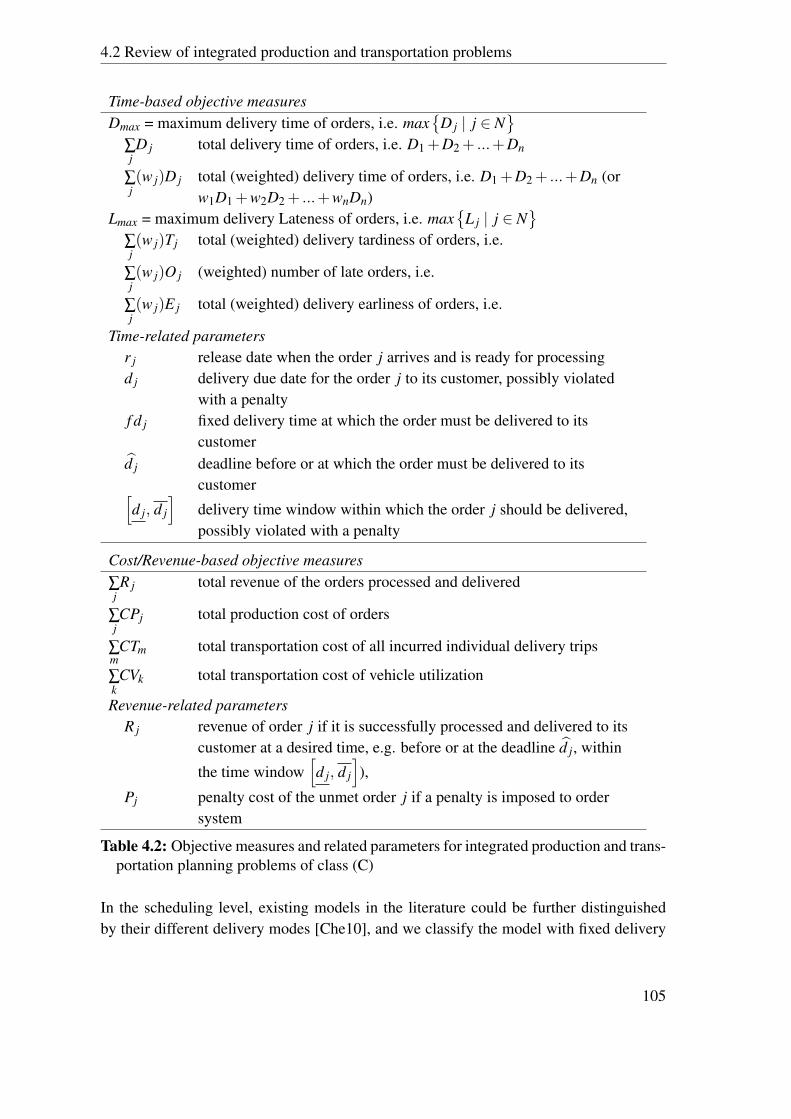
4.2 Review of integrated production and transportation problems
Time-based objective measuresDmax = maximum delivery time of orders, i.e. max
D j | j ∈ N
∑jD j total delivery time of orders, i.e. D1 +D2 + ...+Dn
∑j(w j)D j total (weighted) delivery time of orders, i.e. D1 +D2 + ...+Dn (or
w1D1 +w2D2 + ...+wnDn)Lmax = maximum delivery Lateness of orders, i.e. max
L j | j ∈ N
∑j(w j)Tj total (weighted) delivery tardiness of orders, i.e.
∑j(w j)O j (weighted) number of late orders, i.e.
∑j(w j)E j total (weighted) delivery earliness of orders, i.e.
Time-related parametersr j release date when the order j arrives and is ready for processingd j delivery due date for the order j to its customer, possibly violated
with a penaltyf d j fixed delivery time at which the order must be delivered to its
customerd j deadline before or at which the order must be delivered to its
customer[d j, d j
]delivery time window within which the order j should be delivered,possibly violated with a penalty
Cost/Revenue-based objective measures∑jR j total revenue of the orders processed and delivered
∑jCPj total production cost of orders
∑m
CTm total transportation cost of all incurred individual delivery trips
∑kCVk total transportation cost of vehicle utilization
Revenue-related parametersR j revenue of order j if it is successfully processed and delivered to its
customer at a desired time, e.g. before or at the deadline d j, within
the time window[d j, d j
]),
Pj penalty cost of the unmet order j if a penalty is imposed to ordersystem
Table 4.2: Objective measures and related parameters for integrated production and trans-portation planning problems of class (C)
In the scheduling level, existing models in the literature could be further distinguishedby their different delivery modes [Che10], and we classify the model with fixed delivery
105

Chapter 4 Integrated production and transportation planning with given flexibility
departure method as the 6th mode, listed as below:
• (C.a) Individual and immediate delivery
• (C.b) Batch delivery to a single customer by direct shipping method
• (C.c) Batch delivery to multiple customers by direct shipping method
• (C.d) Batch delivery to multiple customers by routing method
• (C.e) Batch delivery with split delivery method
• (C.f) Fixed delivery departure dates
For models with (C.a) individual and immediate delivery mode, orders need to be deliv-ered individually and immediately after its completion. First studies on individual and im-mediate delivery methods are mostly inspired by [Pot80], in which a modified Schrage’sheuristic algorithm [Sch70] is developed to solve a sequencing problem with n jobs onone single machine and no delivery time window. Woeginger [Woe94] studies a moregeneral version of the problem where there are a set of parallel machines in the plant andgives some heuristics with constant worst-case error bound guarantee. Liu and Cheng[LC02] consider a single-machine scheduling problem with job release dates, deliverytimes, preemption penalties and job-dependent setup. The paper proves that the problemis strongly NP-hard and presents a dynamic programming algorithm and a polynomialtime approximation scheme. Studies of [GH02, WL05] adopt both the branch-and-boundexact algorithm to solve the problem. These mentioned works all concern individual andimmediate delivery problems without time windows. In some problems, a delivery win-dow is imposed in the way that each order j has a fixed delivery time f d j or a delivery
time window[d j, d j
]. With this delivery time window, Garcia and Lozano [GLC04] pro-
pose an exponential-time network based exact algorithm to solve a problem with severalparallel machines at each plant. They also propose a tabu-search based heuristic to solvethe problem.
For models with (C.b) batch delivery to a single customer by direct shipping method,orders come from a single customer zone and each delivery takes the same shipmentroute - from the plant to the customer and goes back. Therefore, each shipment takes thesame delivery route and incurs a same transportation trip time and cost. Chen [Che96]studies a case where a single machine, a common due date shared by all jobs and tominimize the total weighted earliness and tardiness of jobs and total delivery cost. Heconsiders jobs with identical weight respectively on their earliness and tardiness, andprovides a polynomial time dynamic programming algorithm. Sched [Sch01] investigatesvarious problems with a combination of several parameters or conditions: (i) the plant hasa single manufacturing machine, a set of parallel machines, or flow-shop; (ii) the numberof vehicles is limited; (iii) each vehicle can process one or more jobs; (iv) the objective isto minimize either the time when all the delivery jobs are completed (makespan), or the
106

4.2 Review of integrated production and transportation problems
total delivery time of jobs. Many problems are shown to be NP-hard and are commonlysolved with different heuristic approaches, e.g. the problem of [CP06] with a sufficientnumber of vehicles, that of [WC07] with a limited number of vehicles. Some others areshown to be solvable in polynomial or pseudo-polynomial time by dynamic programmingalgorithms, e.g. the problem of [HP03] with an unlimited number of vehicles and that of[HP05] with a limited number of vehicles. The literature mentioned previously in thisparagraph treats the delivered batch in equal size, and quite few papers study problemswith generally different batch sizes [CL04, ZDT07].
Unlike models in (C.b) where each shipment can deliver orders only to one customer, forproblems in the multi-customer category (C.c), different shipments may have differenttransportation routes and costs. This is a more general case than the (C.b) class. Hall etal. [HLP01] study integrated production-transportation scheduling problems with batchdelivery in an arborescent supply chain where a supplier makes deliveries to several man-ufacturers, and manufacturers also make deliveries to customers. Hall and Potts [HP03]solve a (C.c) problem with sufficient vehicles and equal batch size in polynomial time andLi et al. [LVL05] study a one customer subproblem with limited number of vehicles.
Little literature reviewed so far considers vehicle routing decisions. For (C.d) category ofbatch delivery to multiple customers by routing method, only a handful of papers discuss(C) problems involving routing methods. In this category, a shipment is allowed to visitmultiple customer zones and it is necessary to determine the route for each shipment. Arouting problem contains already the strongly NP-hard traveling salesman problem (TSP)[Kap72] as a subproblem, consequently, (C.d) problems are intractable in many cases.
For problems in the category (C.d), Hurter and Van Buer [HVB96, VBWO99] considera joint production and distribution scheduling problem in a newspaper industry. In thiscase, different newspapers are quickly printed in a plant facility during night and thenimmediately delivered to drop off point waiting for delivery carriers to pick them up inthe every early morning. A setup time must be paid between prints of different types ofnewspapers. Demand at each drop off points for different newspapers are known and adelivery deadline d j is given, e.g. 6:30 AM the next morning. The objective is to finda production (printing) schedule and a delivery route for each delivery van involved andthe amount of different type of newspaper to be carried by each delivery van in orderto minimize the number of used vans. Under the assumption that each delivery van canonly be used once, Hurter et al. [HVB96] propose an iterative heuristic to determine thenumber of vans and routings, then based on the routing decisions look for a productionschedule. Under the assumption that each delivery van can be used repeatedly. Further,Van et al. [VBWO99] suggest a local search based heuristics to solve the problem. Liet al. [LVL05] provide a dynamic programming algorithm with deliveries to multiplecustomer locations. Armstrong et al. [AGL08] consider a simple problem where all theorders are processed on a single machine and delivered in a single shipment in a pre-
107

Chapter 4 Integrated production and transportation planning with given flexibility
specified sequence and each order must be delivered within an individual time window[d j, d j
]. The objective is to determine a subset of orders to be delivered so that the total
demand of the delivered orders is maximized. The authors show that their problem is atleast ordinarily NP-hard, and give a branch-and-bound exact algorithm and a heuristic.
Problems in (C.e) batch delivery with split delivery are less explored in existing litera-ture. The study field is, to some extent, superposed to other five classes. Different fromthe “consolidation” indicating whether different orders can be bundled and shipped to-gether in the same vehicle, “split” indicates whether an order is allowed to be split andthen delivered in multiple batches. Thus, splitting refers to delivering the portions of anorder at multiple points in time and may lead to reduced inventory, improvement on ser-vice levels and mitigating the loss or damage during loading and unloading operations.Contrarily, customers may want their orders to be delivered as a whole rather than split,reported by Chen and Pundoor [CP06]. Stecke and Zhao [SZ07] consider a problem ina make-to-order computer manufacturer Dell with two cases : (i) splittable delivery; (ii)non splittable delivery. The authors show that with split mode the problem becomes acost minimization flow problem and is polynomially solvable. With a non-split deliverypolicy, the problem becomes strongly NP-hard and a heuristic is chosen to solve it. Kocet al. [KTS13] examine a manufacturer’s integrated planning problem with three con-siderations: (i) consolidation; (ii) split; (iii) size of orders in terms of vehicle/containercapacities such as full truck load or general load delivery; (iv) heterogeneous vehicleswhere vehicle type I is available in unlimited number in all periods and vehicle type IIonly available at certain period t. The authors propose a dynamic programming runningin pseudo-polynomial time.
For the last category, models with (C.f) fixed delivery departure dates are investigatedby a few papers [WL05, LGS05, LGS06, SZ07]. In this situation, the delivery departuretime of each order is no more a part of decision, but a part of input data. Wang and Liang[WBJS05] study a coordinated mail processing and distribution scheduling problem ata mail processing and distribution center with heterogeneous vehicles. The objective isto minimize the total un-used truck capacity. Some dispatching rules are proposed andthe problem is solved by heuristics. Stecke and Zhao [SZ07] consider also the problemof a make-to-order situation where each order is limited with a delivery time deadline.Heterogeneous vehicles are taken into account with a decreasing shipping time and alinear function of order size. In their problem, a number of delivery modes exists butvehicles have fixed departure dates.
4.2.4 Further prospects
We have reviewed existing models on integrated production and transportation problemsby three macro categories (A-B-C), and six sub class for the third class (C) of integrated
108

4.2 Review of integrated production and transportation problems
production and outbound distribution scheduling problems. These classes of the litera-ture address various practical situations in the production-transportation area and provideuseful problem-solving methods. The majority of the work was done in the last decades,indicating a growing interest in this study field.
Besides, much more research is needed for further studies and for some relatively newareas:
• Problems with heterogeneous vehicles. Only a handful of papers [WL05, SZ07,KTS13] consider heterogeneous vehicle issues in their work, while the heteroge-neous vehicle delivery mode occurs in many applications and deserves more re-search attention. Different kinds of vehicle may have the same or different capacitywith different delivery speeds and costs, and many package delivery services of-fered by third party logistics (3PL) may provide overnight, one-day, two-day deliv-ery with different costs. The problems with heterogeneous vehicle are worth moreresearch attentions because of its practical relevance.
• Problems with stochastic demand. Most existing results consider deterministicmodels where product demand is known in advance to satisfy with or without back-logging. However, many products in practice does not figure in this field. Forproducts having a large variety with short life cycle, the customer demand is ofhigh uncertainty and difficult to predict. In this case, stochastic demand or with acertain distribution may be more realistic to reflect the industrial world.
• Problems with non-linear costs. Most production-transportation problems reviewedin this section involve linear transportation costs, which may be unrealistic in indus-try. The transportation cost is normally nonlinear in practice (e.g. fixed charge plusvariable nonlinear charge). Thus, problems with non-linear costs are well worthyof further investigations.
• Value of coordination. The coordination between production and transportation isimportant but has a cost. Quite few papers [CF94, FV99] have studied the valueof coordination between production and distribution phases. If one can quantifytheoretically the value of coordination for some general models, we can decidewhether it is worthwhile to optimize production and transportation jointly, and ifyes, to which extent they can be coordinated.
• Integrated scheduling problems with routing decisions. In our review, this class ofproblems is referred to as problem class (C.d) “batch delivery to multiple customersby routing method” and is difficult to solve. Most reviewed studies involve unlim-ited number of homogenous vehicles, and it would be worthwhile to provide studieswith multiple and number-limited vehicles. Furthermore, many companies practiceJIT manufacturing policy and require frequent delivery of small quantities. Withmultiple customers locating in different zones, it would be necessary to consolidate
109
Chapter 4 Integrated production and transportation planning with given flexibility
orders of some customers to save transportation cost. Therefore, it is worthwhileto consider routing methods involving different destinations across multiple trans-portation stops. To solve such problems, it is important to exploit problem structureto reduce the algorithm complexity. Fast and robust solution algorithms need to bedeveloped for large scale problems.
110

4.3 Problem description for Evian
4.3 Problem description for Evian
We propose models and algorithms to solve the integrated production and transportationplanning problem, with a particularity of incorporating several given flexibilities. In theliterature mentioned above, few literature incorporates the flexibility consideration di-rectly into the model. But nowadays, it is important for firms to arrange their industrialactivities to achieve the final commercial goal, also commonly under some certain flexi-bility tolerances, which may be contracted with supply chain partners or stemmed fromtheir internal decisions. For this, we put our eyes here inside a case study with the Frenchmineral water company, Evian.
Evian is owned by Danone Group, a French multinational company. The brand Evian isthat of luxury mineral water coming from several sources near Evian-les-Bains of depart-ment Haute-Savoie, on the south shore of Lake Geneva. Evian water is the most sold inFrance, UK, Belgium, Switzerland, well placed as imported water in the United Statesand especially in Japan.
Figure 4.5: Warehouses in Evian problem
In Evian itself, the manufacturing activity studied in this work starts from producing bot-tle pre-forms, then blowing them in various formats, bottling water and getting packagesfinished in several production lines until completing the palletization. This can be to-tally regarded as a continuous production activity, while the stock keeping unit (SKU)is defined as a combination of bottle format and market zone. Stock is held by variouswarehouses (most warehouses are near ports) and no stock on-site, as shown in Fig.4.5.
111

Chapter 4 Integrated production and transportation planning with given flexibility
Therefore, finished goods must be rapidly transferred by trains or trucks to warehousesafter production (so called “deployment”), waiting to be dispatched to corresponding re-gions. In Evian case, there are 14 production lines, 9 warehouse destinations and about420 SKU. The flexibility problem also lies in transportation activity with trains and trucks,because trains must be reserved 3 months before departure according to contracts withtrain operators. Any exceeding or cancellations may generate a prohibitive cost. Besides,available trucks are also limited. Thus, we are quite aware of heterogeneous vehicles usedin our problem. This transportation deployment is shown in Fig.4.6.
Figure 4.6: Production and transportation activity in the mineral water company
The close linkage between production and transportation, and the deployment of productsby two transportation modes lead to a great need of possible modifications in productionplanning to meet the transportation constraints. Indeed, some fluctuation is possible forthe train reservation, but only a small scale of flexibility is allowed. Though train trans-portation does manifest this or that disadvantage, the advantages are clear and strong.First, cost of railway transportation is relatively low compared with truck prices, partic-ularly if a railway track is already built up between two locations. Secondly, the finalproducts of Evian are bottled water in different formats, which are still heavy and mustbe delivered in a large amount. Thus, a truck may leave the production site with only onethird of its volume filled up, for the reason that its weight reaches the maximum allowanceof highway. Thirdly, train is a mode of transportation with less emission of CO2, there-fore, cleaner and greener than other freight transportation modes. This is very important,because Evian prefer to show that its water production is clean and green and does not leadto too much pollution to the environment. Fourthly, all the train wagons waiting on therailway track can serve as storage area, store bottled water and ship them away directly.Therefore, in the Evian case, we appreciate and put priority to train transportation.
112

4.3 Problem description for Evian
In this problem, two goals are expected by the company manager to be simultaneouslyachieved:
• Bring inventory level for each SKU over all warehouses to their target interval, inorder words, as close as possible to an interval [stock Target ~ stock Max]
• Coordinate production plan and transportation plan as close as possible and givepriority to train transport, which indicates that the fill rate of train wagons may beefficiently maximized
To achieve both main goals, we propose a cost-based model to include the minimizationof inventory penalty, which is different from inventory holding cost. This penalty is theadditional cost for each SKU for any deviation from the stock target, with a cost structureillustrated in Fig.4.7. C−, C0 and C+ in the figure are linear penalty coefficients to be setrespectively for the inventory level under target value, in the interval of target-maximumor beyond the maximum value. In this way, the cost structure aims at penalizing heavilythe deviation from the flexible target interval and slightly the inventory holding above thetarget minimum value.
Figure 4.7: Penalty curve for the inventory policy
Among all production lines, some are capable of producing more than one SKU or severalfamilies of SKUs. Therefore, changeover is allowed but requires quite a long time toswitch between SKUs. Except for some special SKUs, changeover (setup) cost must bepaid for each batch if a changeover occurs between different families. Only the setup costand time among SKUs within a same family could be considered to be negligible.
So the objective of this study is to provide a production and transportation plan in details,respectively described as follows:
Production plan
• Quantity of SKU to produce on production line k in period t
113

Chapter 4 Integrated production and transportation planning with given flexibility
• Changeovers between SKUs on production line k in period t
Transportation Plan
• Number of trains used in direction of warehouse l in period t
• Number of trucks to direction of warehouse l in each period t
This study concentrates on medium/short-term planning, but does not work on schedulingdetails. That means, changeovers for SKUs i, j at a time period needs to be determined andspecified but will not be determined in a detailed time period and in a determined sequencein our solution. This work consider that all data are deterministic. Other assumptions forthe studied problem are listed as below:
1. Forecast (demand) is assumed to be accurate and deterministic for each planningperiod consisting of demands per SKU
2. Production capacity for each production line of the plant is a deterministic value ineach planning period
3. Inventory level taken into account in the model of product i is the summation ofinventory over all warehouses for each SKU i
4. Unmet demand is backordered with a penalty and the inventory level turns negative
5. Products in transit (in transportation) is counted for inventory level
6. Initial inventory at t0 is set to the minimum target value
7. Each SKU can only be packed and transported in proper pallet, coded with the sameindex
8. There may be more than one changeover between SKUs for each production line kin a period
9. Changeover from each specific SKU i to another specific SKU j on specific line kcan only occur once in each period, which is consistent with the real situation of thecompany
Particularly, flexibility considerations in this problem could be listed as below:
1. Inventory target interval is flexible [stock Target ~ stock Max] with a certain variablecost
2. Transport allocation of SKUs among warehouses has certain flexibility
3. Various pallets of different dimensions can be transported in the same wagon or thesame truck
4. A limited degree of flexibility for the number of trains is available in each planningperiod
114

4.4 Model with average transport cost (ATC) to solve Evian problem
4.4 Model with average transport cost (ATC) tosolve Evian problem
4.4.1 Mathematical formulation
In this section, the problem at hand is formulated mathematically into a mixed integerlinear program. The first objective is to minimize the total cost generated from productionchangeover, inventory holding and train and truck utilization, with an average transportcost per pallet taken into account. If more than one solution with the same value ofobjective function are found, the one which deploys the fewest trucks will be chosen.This indicates the priority on train utilization and less stocks in transit by trucks. Thismodel with Average Transport Cost, can be indexed as model ATC for short.
According to contracts with the third part transporters of Evian, no other fixed cost isconsidered if the number of trains is kept in
[W lt ,W lt
]for destination l (warehouses or
direct market zones) and period t, which can be fractionated to several wagons. And dueto lack of information, only the average transport data by pallet proposed by the studiedcompany is available for transportation cost by train CostTl , and transportation cost bytruck CostCl for destination l. The average quantity for pallets per wagon and per truckis adopted to keep the model in linear form, which coincides with statistics of the studiedcompany. Furthermore, for each produced SKU, it can be transported to l destinationsin a fluctuated percentage, varying in an interval
[Pil,Pil
]. All these constitute the main
given flexibilities of the problem.
Decision variables and parameters are listed as follows:
Decision Variablesxikt production quantity of SKU i on production line k in period tzilt quantity of SKU i transported to warehouse l in period tyi jkt binary variable indicating whether a setup is needed from SKU i to
SKU j on production line k in period tIit inventory amount for SKU i at the end of planning period tNWlt number of wagons to reserve in direction of warehouse l in period tNClt number of trucks to order in direction of warehouse l in period t
Table 4.3: Decision variables for integrated production and transportation planningproblem
115
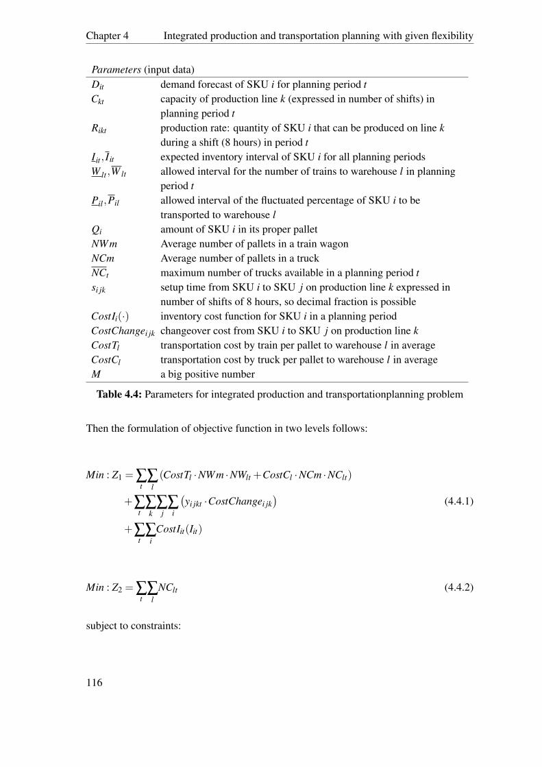
Chapter 4 Integrated production and transportation planning with given flexibility
Parameters (input data)Dit demand forecast of SKU i for planning period tCkt capacity of production line k (expressed in number of shifts) in
planning period tRikt production rate: quantity of SKU i that can be produced on line k
during a shift (8 hours) in period tIit , Iit expected inventory interval of SKU i for all planning periodsW lt ,W lt allowed interval for the number of trains to warehouse l in planning
period tPil,Pil allowed interval of the fluctuated percentage of SKU i to be
transported to warehouse lQi amount of SKU i in its proper palletNWm Average number of pallets in a train wagonNCm Average number of pallets in a truckNCt maximum number of trucks available in a planning period tsi jk setup time from SKU i to SKU j on production line k expressed in
number of shifts of 8 hours, so decimal fraction is possibleCostIi(·) inventory cost function for SKU i in a planning periodCostChangei jk changeover cost from SKU i to SKU j on production line kCostTl transportation cost by train per pallet to warehouse l in averageCostCl transportation cost by truck per pallet to warehouse l in averageM a big positive number
Table 4.4: Parameters for integrated production and transportationplanning problem
Then the formulation of objective function in two levels follows:
Min : Z1 = ∑t∑
l(CostTl ·NWm ·NWlt +CostCl ·NCm ·NClt)
+∑t∑k∑
j∑
i
(yi jkt ·CostChangei jk
)(4.4.1)
+∑t∑
iCostIit(Iit)
Min : Z2 = ∑t∑
lNClt (4.4.2)
subject to constraints:
116

4.4 Model with average transport cost (ATC) to solve Evian problem
Ii(t−1)+∑k
xikt− Iit = Dit ∀i,∀t (4.4.3)
∑i(zilt/Qi)≤ NWlt ·NWm+NClt ·NCm ∀l,∀t (4.4.4)
∑i[(1/Rikt) · xikt ]+∑
i∑
j
(yi jkt · si jk
)≤Ckt ∀k,∀t (4.4.5)
xikt ≤M ·∑j
y jikt ∀i,∀k,∀t (4.4.6)
∑k
xikt = ∑l
zilt ∀i,∀t (4.4.7)
W lt ≤ NWlt ≤W lt ∀l,∀t (4.4.8)
zilt ≥ Pil ·∑k
xikt
zilt ≤ Pil ·∑k
xikt∀i,∀l,∀t (4.4.9)
∑l
NClt ≤ NCt ∀t (4.4.10)
yi jkt = 0,1 ∀i 6= j,∀k,∀t (4.4.11)
xikt , zilt , NClt ≥ 0 ∀i,∀ j,∀k,∀t (4.4.12)
117

Chapter 4 Integrated production and transportation planning with given flexibility
In Eq. (4.4.1), the objective Z1 minimizes the sum of four types of cost for train plan,truck plan, production changeover plan and inventory penalty values.
In particular, corresponding to the stock penalty structure in Fig.4.7, costs in the fourthterm StockCost = ∑
t∑iCostIi(Iit) of Z1 is formulated from the piecewise function to a
maximum group (4.4.13), which adds penalty cost to stocks deviating from the targetinterval. C−, C0 and C+ are cost coefficients for the inventory level respectively undertarget value, in the interval of target-maximum or beyond the maximum value. For theEvian case, we have decided to configure C− =−2, C0 = 1/4 and C+ = 2, and thus forma penalty curve presented in Fig.4.7.
CostIit(Iit)≥
C− · (Iit− Iit)
C0 · (Iit− Iit)
C+ ·(Iit− Iit
)+C0 ·
(Iit− Iit
) ∀i,∀t (4.4.13)
The second objective, marked as relation (4.4.2), minimizes the utilized trucks and claimsthe priority of transportation allocation by train if there are alternative solutions foundfor objective value (4.4.1). This also interprets less stock in transit by trucks. If othersolutions with similar objective value are not found, (4.4.2) can be omitted referring toalgorithm step 1) in sec.4.4.2. Inventory flow conservation per SKU is shown in rela-tion (4.4.3), where backorders are allowed instead of lost sales with a negative value inIit during T planning periods. It is noticeable that in this formulation, Iit does not dis-tinguish between physical stock in each warehouse and stock in transit (in transport towarehouses); so ∑
kxikt just bring the two into consideration. Flow conservation by ware-
houses per SKU is expressed in (4.4.4), which sums up total numbers of SKU’s palletstransported by trains and by trucks. It also indicates that all production of any SKU i inany period t must be transported to warehouses during the same period, this express thefact that there is no on-site storage area. Capacity constraints are expressed in relation(4.4.5) to ensure that time length consumed by SKU production and SKU changeover,does not exceed the capacity of any production line. For the SKUs cannot be producedon line k in period t, value 0 is assigned to their production rate Rikt . Eq. (4.4.6) deter-mines if a SKU is produced in period t on line k, the corresponding setup must be paid. Ifchangeovers cannot occur on line k, a big positive value M is assigned to their setup timessi jk and costs CostChangei jk to prevent from setting up. Eq. (4.4.7) ensures the sum ofproduction quantity xikt of SKU i on production line k is identical to that of productionquantity zilt of SKU i transported to warehouse l in each period.
Flexibility is always in our concern. The fluctuation range for train is declared by relation(4.4.8) to restrict the number of trains into a flexible interval. Different train may con-tain different number of wagons. Furthermore, to transport products to destinations, the
118

4.4 Model with average transport cost (ATC) to solve Evian problem
company allocates the delivery of SKU i to different direction l in a percentage, within afluctuated interval
[Pil,Pil
], expressed in Eq. (4.4.9). Eq. (4.4.10) claims the maximum
number of trucks available in each planning period, including round trip trucks. These areall involved in flexibility considerations. In the end, constraints (4.4.11) and constraints(4.4.12) are to show the feasibility conditions of variables.
When production and transportation plans are determined, fill rates T f illlt of train andC f illlt of truck can be approximately calculated. If N pTi denotes the maximum quantityof pallets of type i in a wagon and N pCi for that in a truck, fill rates could be formulatedas below:
T f illlt = ∑i
∑k
xikt ·NWm
Qi ·N pTi · (NWm ·NWlt +NCm ·NClt)∀l,∀t
(4.4.14)
C f illlt =
∑i
[∑k
xikt/(Qi·N pCi)
]NClt
·100%
i f NWlt = 0,NClt > 0
∑i
∑k
xikt ·NCm
Qi·N pTi·(NWm·NWlt+NCm·NClt)·100%
i f NWlt > 0,NClt > 0
∀l,∀t (4.4.15)
4.4.2 Solution algorithm - heuristic
In the previous review on integrated production and transportation planning problems,this kind of capacitated mixed-integer problem is proved to be complicated in solving,and may require a great amount of computation time to find an optimal solution withtraditional branch-and-bound algorithms. In this work, a problem-specific heuristic algo-rithm based on “Improvement” logic is proposed to solve the problem, and proved to beefficient to find the solution in a reasonable amount of time.
First, to accelerate the computation of the proposed heuristic, the maximum costs CostIi(Iit)
in group relation (4.4.13) are discarded, which are only used to program with CPLEX inorder to compare with the proposed algorithm. In our heuristic, the cost CostIi(Iit) is
119

Chapter 4 Integrated production and transportation planning with given flexibility
turned into a piecewise function (4.4.16) in order to calculate the inventory cost directlywith different thresholds, while the old one remains in relation (4.4.13) to calculate solu-tions with the help of CPLEX.
CostIit(Iit) =
C− · (Iit− Iit) Iit < IitC0 · (Iit− Iit) Iit < Iit
C+ ·(Iit− Iit
)+C0 ·
(Iit− Iit
)Iit ≥ Iit
∀i,∀t (4.4.16)
In a summary, the proposed algorithm can be divided into two parts: Construction - find-ing the first feasible solution, and Improvement - searching for a near-optimal solution.In the construction phase, we first generate an initial production and transportation planaccording to the demand on different SKU, and adopt the first plan with minimum valueon number of trains. This initial solution may be infeasible because the capacity of trainand the capacity of truck can be violated. The next step is to adjust this plan with respectsto concerning constraints to obtain the first feasible solution. In this context, the coreelement is that the initial plan is set with minimum train numbers in different direction(destination), which guarantees a starting point at objective value Z1 as low as possibleand leads to a fast solution exploration. After that, we focus on objective function (4.4.1)and look for the big terms with big coefficients in order to reduce big costs to reach bettersolutions. Finally, we proceed into the comparison phase to terminate this solution explo-ration. The objective value Z2 is used to compare with other solutions if there exist morethan one solution with similar cost on objective value Z1.
This algorithm is generally illustrated in Fig.4.8 in the next page. In the next subsections,we describe all the small loop of our heuristic in detail.
120

4.4 Model with average transport cost (ATC) to solve Evian problem
Figure 4.8: General algorithm of the heuristic to solve the integrated production andtransportation problem - model ATC
4.4.2.1 Construction: first feasible solution
To obtain a feasible solution as the starting point, we first generate an initial plan which isnot necessarily feasible. After that, the concerning constraints which have not been usedto generate the initial plan are examined, in order to adjust the production and transporta-tion decision variables to feasible ones.
121

Chapter 4 Integrated production and transportation planning with given flexibility
After the adjusting operations, constraints are reviewed to check whether all conditionsare met; if not, go back to the adjusting phase; otherwise, a feasible solution is found andis stored, indexed as Sl0 in the solution collection ∑. All variable values are stored andthe objective values Z1 and Z2 are calculated as upper bound for the next step. This isdetailed in Fig.4.9.
In Fig.4.9, the key idea of construction phase is to generate an initial production plan in arough and set all trains to their minimum numbers. This process is extremely fast, basedon good knowledge of the problem-specific data properties. For the products that cannot be transported by inital numbers of train wagons, we first seek help from availabletrucks to transport them. If train numbers are well within reach (remaining in
[W lt ,W lt
]),
the feasible initial transportation plan comes out directly; if not, the algorithm turns backto modify train numbers (incrementation only). If the train and truck maximum valuesare all reached and violated, try to change the delivery distribution
[Pil,Pil
]in different
direction (destination) to balance the transportation. And if the delivery balancing couldnot give out a satisfied transportation plan, the corresponding production quantity xikt isto be adjusted. Normally, we go quite fast to acquire the first feasible solution.
Figure 4.9: Construction for the first feasible solution - model ATC
122

4.4 Model with average transport cost (ATC) to solve Evian problem
4.4.2.2 Improvement: search for a near optimal solution
Based on the feasible solution obtained in the previous phase, the exploration of a near-optimal solution can be carried out in the same logic. Here the objective function valuesZ1 and Z2 play important roles, since the algorithm detects terms of big value with thelargest coefficients in Z1 to reduce the total cost, among the terms A, B, C and D for fourmain costs in our objective function.
The four cost terms A, B, C and D are presented in the following figures, illustrated indetail in Fig.4.10 with cases A and B, and continued in Fig.4.11 with C and D. A smallalgorithm bloc “Bloc P” is illustrated in Fig.4.11. If the algorithm exploration comes upto “Bloc P” on the left of Fig.4.10, or on the bottom of Fig.4.11 (“Bloc P in Case A”), thealgorithm enters directly the small algorithm Bloc P for further computation.
The algorithm is quite detailed in the following algorithms, but the real logic is simple.Each time when a decrease or increase of the cost term occurs, the concerning constraintslinked by decision variables in this term will be immediately retreated. In order to keepthe conservation of constraints, the algorithm may arrive to additional reduction or incre-mentation for other variables. For instance, inventory Iit and changeover yi jkt are closelylinked: if Iit is modified, the corresponding changeover yi jkt must be checked, or evenmodified. The same thing happens to the numbers of train NWlt and truck NClt . For thosetransportation cost terms, the mutual linkage is mainly determined by delivery distribu-tion in their transport modes (train/truck). And, the problem-specific algorithm coding inVB.net has exploited the problem’s data properties to avoid useless exploration so as toget directly to the next step.
123

Chapter 4 Integrated production and transportation planning with given flexibility
Figure 4.10: Improvement for next feasible solution for model ATC - part I
124

4.4 Model with average transport cost (ATC) to solve Evian problem
Figure 4.11: Improvement for next feasible solution for model ATC - part II
125
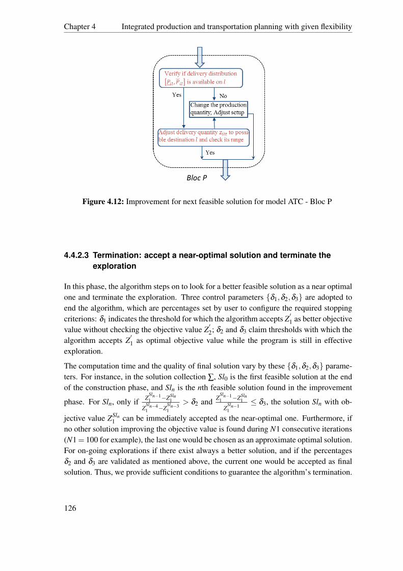
Chapter 4 Integrated production and transportation planning with given flexibility
Figure 4.12: Improvement for next feasible solution for model ATC - Bloc P
4.4.2.3 Termination: accept a near-optimal solution and terminate theexploration
In this phase, the algorithm steps on to look for a better feasible solution as a near optimalone and terminate the exploration. Three control parameters δ1,δ2,δ3 are adopted toend the algorithm, which are percentages set by user to configure the required stoppingcriterions: δ1 indicates the threshold for which the algorithm accepts Z
′1 as better objective
value without checking the objective value Z′2; δ2 and δ3 claim thresholds with which the
algorithm accepts Z′1 as optimal objective value while the program is still in effective
exploration.
The computation time and the quality of final solution vary by these δ1,δ2,δ3 parame-ters. For instance, in the solution collection ∑, Sl0 is the first feasible solution at the endof the construction phase, and Sln is the nth feasible solution found in the improvement
phase. For Sln, only if ZSln−11 −ZSln
1
ZSln−41 −Z
Sln−31
> δ2 and ZSln−11 −ZSln
1
ZSln−11
≤ δ3, the solution Sln with ob-
jective value ZSln1 can be immediately accepted as the near-optimal one. Furthermore, if
no other solution improving the objective value is found during N1 consecutive iterations(N1= 100 for example), the last one would be chosen as an approximate optimal solution.For on-going explorations if there exist always a better solution, and if the percentagesδ2 and δ3 are validated as mentioned above, the current one would be accepted as finalsolution. Thus, we provide sufficient conditions to guarantee the algorithm’s termination.
126

4.4 Model with average transport cost (ATC) to solve Evian problem
4.4.3 Computational Results
The computation is performed using a Dell Optiplex 780 computer with an Inter CoreDuo 2.66 GHz Processor and 3.21 Go RAM under 32 bit WindowsXP environment. Theproposed heuristic for the linear problem described in the previous sections was codedin language VB2005 (VB.net) with original data provided by the company in Excel files.When using Cplex of Ilog Cplex version 11.1 to solve the model to compare with ourheuristics, we put weights on the two objectives Z1 and Z2 to merge into a single objectivefunction. This case study makes use of the real input data from the Evian company. Asdescribed in section sec.4.3, the results are presented in production plan and transportationplan. For reason of confidentiality, only an extract of results can be shown in table Tab.4.5and in table Tab.4.6.
Tab.4.5 gives out a production plan extracted from our output results, which specifies howmany thousand bottles to produce in which production line in which period by SKU. Forexample, the SKU coding as 12424 in family EV50CT24 is proposed to produce 219,000bottles in the fifth week. Tab.4.6 gives out a train transportation plan, which specifieshow many trains should be ordered in which direction in a period. For example, twocomplete trains must be reserved for warehouse Boulogne in the fourth week, and twoand a half trains for Le Havre in the sixth week. For the direction to Le Havre, an entiretrain contracted with SNCF is composed by 28 wagons, that is, 2.5 trains = 70 wagonscommanded.
On the one hand, since we do not have the detailed real production data by SKU providedby Evian, the comparison of the production plan with the real one is omitted. On theother hand, the transportation planning data is available for the first eight periods (week)in 2011 provided by Evian, shown in Tab.4.7. So the transportation plan can be compared.
In this table, the column 2 and 3 denote the minimum and maximum values of trainnumber, and if the corresponding transportation deployment by train does not violate thisinterval, the cell of train number is colored in green. If it exceeds the number, coloredin purple, else if it is smaller than the minimum value, colored in red. The data fromEvian reveals its clear deficiency on transportation plan, since there are a lot of shortagesand surplus. Whereas, our output results in Tab.4.6 have better arranged the train planin the expected interval, and at the same time, the total truck numbers are smaller andmore stable than those from Evian. The train number and truck number are not only theresult of transportation planning but also the result of production planning. In this way,comparison between the two transportation tables confirms that our approach works wellto provide good integrated production and transportation plans.
127

Chapter 4 Integrated production and transportation planning with given flexibility
Table 4.5: Output production plan for Evian problem - model ATC
Table 4.6: Output transportation plan for Evian problem - model ATC
Nevertheless, tests are carried out to compare the solution qualities and computation timeswith three algorithms: the proposed heuristic, the CPLEX program and the heuristic-CPLEX combined method.
The first algorithm is the suggested problem-specific heuristic, tested here with two sets ofcontrol thresholds δ = δ1,δ2,δ3 in δ 1 = 6%,90%,0.02% and δ 2 = 3%,95%,0.005%,which are presented in sec.4.4.2.3.
The second one exploits the mixed integer optimizer of ILOG CPLEX, in which two ob-jective functions are merged into a single one by a weighting system. CPLEX MIP solveruses the branch-and-bound technique to obtain an optimal solution. Since the train uti-lization is of the first priority, the objective Z1 is roughly weighted 200 times than Z2.Theoretically if we do not set any termination limits such as number of nodes, time, ...,
128

4.4 Model with average transport cost (ATC) to solve Evian problem
Table 4.7: Transportation plan data provided by Evian
we could wait until the termination of the algorithm by finding final solution with guar-anteed optimality. However, its optimality is sometimes relative to whatever tolerancesand optimality criteria the user has set. For instance, CPLEX considers any user-suppliedcutoff value (such as CutLo or CutUp) as well as the objective difference parameter (Ob-jDif) when it treats nodes during branch and cut; thus these settings affect terminationindirectly.
The third algorithm is the heuristic-CPLEX combined method. It is more interesting, aswe introduce initial feasible solution generated by the suggested heuristic as the startingfeasible solution of CPLEX program (set MipStart=1 to load the solution then use othertechniques to refine the solution). This is a combined approach; we theoretically expect itto be more efficient.
Table 4.8: Comparison on objective value and run time for three algorithmsin Model ATC
129

Chapter 4 Integrated production and transportation planning with given flexibility
Tab.4.8 shows the comparison on objective value and computation time respectively forthe mentioned three algorithms. The first column marks the scenario datasets: for setSKU50, where input data involve only 50 SKUs on 3 production lines for 4 warehousedestinations in 12 weeks; 100 SKUs on 6 lines to 5 warehouses for SKU100 in 12 weeks;200 SKUs on 7 lines to 8 warehouses for SKU200; 420 SKUs on 14 lines to 14 ware-houses; 840 SKUs on 20 lines to 14 warehouses. Meanwhile, integer variables are alwaysnumerous. For heuristic column, the results are listed in termination criterion δ 1 and δ 2,mentioned in the paragraph above. For objective value column, Z1 is the total cost ineuros and for time column in CPU seconds.
From these results, we would conclude that the CPLEX optimizer provides the optimalsolution, at a cost of consuming enormous amount of time due to the large number ofinteger variables, even in condition that a large number of integer variables are set to0 according to some knowledge in modeling. For set SKU840, CPLEX cannot achievethe optimal solution in a reasonable amount of time and even for SKU420, it consumesa big amount of computation time. In contrary, the suggested heuristic shows a goodperformance to provide an approximate solution in very short time. A few minutes areenough to complete computing for set SKU420, while CPLEX encounters difficulties tolook for the next feasible solution. It is also observed that the quick termination δ 1 reallycomputes more speedily than δ 2, and provides similar results. We can change δ sets toget better solutions. The backorder cost is not counted in the objective function, but canbe compensated by inventory penalty cost. In the proposed heuristic algorithm, backorderis rarely increased and only used to compensate small unequal amount; in the CPLEXmethod, it is a little hard to anticipate even if there is an inventory penalty evaluationto prevent from stock-out. Moreover, in the last column, the Gap represents the relativeerror of the heuristic solutions with respect to the optimal solutions provided by CPLEX.It can be observed that the Gap increases slightly as long as the problem size increases,however, the Gap observed are always insignificant when comparing the total cost againstthat of the optimal solution. For termination δ 1, relative errors are greater that those ofthe termination δ 2 with less computation time, but, still under 0.1%. For terminationδ 2, relative errors can be observed as tiny gap (<0.05%). This shows that the proposedheuristic is well efficient to seek for solutions with good quality.
In the column “Heuristic + CPLEX” of Tab.4.8, it is observed that the heuristic feasiblesolution followed by CPLEX program can reduces significantly the computation time,while providing a solution with similar quality to that obtained with the unique CPLEXoptimizer. In fact, there is a slight difference in objective value for the scenario SKU200,due to different refining actions after loading the initial solution, which may lead to smalldifferences on optimality. Nevertheless, its run time is still too long for a weekly planningsolution. For a small size problem, the combined method is pretty good to substitute thetraditional branch-and-bound algorithm. For a planning problem over 12 weeks updated
130

4.4 Model with average transport cost (ATC) to solve Evian problem
each week with tremendous integer variables, it is worthless to look for a solution withguaranteed optimality in such a long horizon. In this way, the suggested problem-specificheuristic works more efficiently.
131

Chapter 4 Integrated production and transportation planning with given flexibility
4.5 Model with variable transport cost (VTC) tosolve Evian problem
In the previous model ATC, average quantity of pallets per wagon and per truck is adopted,to fill the wagon and the truck space in order to linearize the objective function. Evenif the company approves this method, it is not accurate enough. After searching for asatisfactory solution, the algorithm releases a production plan and a transportation plan,but the number of pallets of bottles filled in train wagons or inside a truck is still unclear indetail. It is necessary to introduce additional modified variables substituting the averagenumber of pallets by train wagon and by truck, and the proposed heuristic can be slightlymodified to obtain results with much more precision.
4.5.1 Mathematical formulation
In addition to the preceding model ATC, the input data NWm representing the averagenumber of pallets by train wagon and NWc the average number of pallets by truck, areeliminated. The fixed costs of utilization of train wagon and truck are completely sepa-rated from these pallet-average costs. As a result, transportation cost is explicitly dividedinto a fixed cost by train and by truck plus a variable cost relative to the number of pallets.Apart from the parameters for model ATC, volume data for each SKU pallet, train wagonand truck are the input data added into the new parameter list:
ParametersV Tl Wagon volume in m3
VCl Truck volume in m3
Vi Pallet volume in m3 for each SKU iα maximum fill rate for a truck in volume (relative to the maximum
loading allowance on auto-routes)CostT Fl fixed transportation cost per train to warehouse lCostTCl fixed transportation cost per truck to warehouse l
Table 4.9: New parameters for integrated production and transportation problemin model VTC
Different from the previous model, the former decision variable zilt is splitted into twobranches with index c = 1,2 to provide more precision:
132

4.5 Model with variable transport cost (VTC) to solve Evian problem
Decision Variableszilct Production quantity of SKU i to be transported by train (c = 1) or by
truck (c = 2) to destination l in period t
Table 4.10: New decision variables for integrated production and transportationproblem in model VTC
With these modifications, the model with average transport cost (ATC) can be transformedto a model with Variable Transport Cost (VTC). Then the formulation of objective func-tion in two levels of the model with variable transport cost (VTC) follows:
Min : Z1 = ∑t∑
l
(CostTl
Qi·∑
c=1zilct +CostT Fl ·NWlt
)
+∑t∑
l
(CostCl
Qi·∑
c=2ziclt +CostTCl ·NClt
)(4.5.1)
+∑t∑
i∑
j∑k
(yi jkt ·CostChangei jk
)+∑
t∑
iCostIit(Iit)
Min : Z2 = ∑t∑
lNClt (4.5.2)
subject to modified constraints, compared with the model in average transport cost:
Ii(t−1)+∑l∑c
zilct− Iit = Dit ∀i,∀t (4.5.3)
∑i
(∑c
zilct/Qi ·Vi
)≤ NWlt ·V Tl +NClt ·α ·VCl ∀l,∀t (4.5.4)
∑k
xikt = ∑l∑c
zilct ∀i,∀t (4.5.5)
133

Chapter 4 Integrated production and transportation planning with given flexibility
∑c
zilct ≥ Pil ·∑k
xikt
∑c
zilct ≤ Pil ·∑k
xikt∀i,∀l,∀t (4.5.6)
xikt , zilct , NClt ≥ 0 ∀i,∀ j,∀k,∀c,∀t (4.5.7)
subject to additional constraints for vehicle mode index c = 1,2, compared with themodel in average transport cost:
∑i(zil1t/Qi ·Vi)≤ NWlt ·V Tl ∀l,∀t (4.5.8)
∑i(zil2t/Qi ·Vi)≤ NClt ·α ·VCl ∀l,∀t (4.5.9)
The other constraints remain the same with relations in the previous section in Eq. (4.4.5),Eq. (4.4.6), Eq. (4.4.8), Eq. (4.4.10) and Eq. (4.4.11).
In view of Eq. (4.5.1) in this model, the objective Z1 minimizes the sum of four types ofcost for train plan, truck plan, production changeover plan and inventory penalty values.Transportation cost is clearly divided into fixed and variable cost per train and fixed andvariable cost per truck. Corresponding to the stock penalty structure in Fig.4.7, costs inthe fourth term StockCost = ∑
t∑iCostIi(Iit) of Z1 remain the same as a maximum group
constraints (4.4.13) adding penalty cost to corresponding inventory.
The second objective marked as relation (4.5.2), remains the same and minimizes theutilized trucks. If other solutions with similar objective value are not found, (4.5.2) can beomitted referring to algorithm step 12) in section sec.4.4.2. Inventory flow conservationper SKU is shown in relation (4.5.3), where backorders are allowed instead of lost salesduring T planning periods and so Iit can be negative. As Iit does not distinguish betweenphysical stock in each warehouse and stock in transit (in transport to warehouses), theterm ∑
l∑c
zilct just bring the two into consideration. Flow conservation by warehouses per
SKU is expressed in volume conservation in (4.5.4), which sums up the total volume ofSKU’s pallets transported by trains and by trucks. This relation can be divided into twoparts: train flow (4.5.8) with c = 1 and truck flow (4.5.9) with c = 2. For the truck flow,the truck utilization are not only limited by its volume capacity but also by loading weight
134

4.5 Model with variable transport cost (VTC) to solve Evian problem
on road, which refers to only one third of its volume fulfilled in the Evian case, that meanswe choose the parameter α = 1/3 in Eq. (4.5.4) and Eq. (4.5.9). Moreover, Eq. (4.5.5)ensures the sum of production quantity xikt of SKU i on production line k is identical tothe sum of ∑
czilct for SKU i to be transported to warehouse l in each period. To transport
products to corresponding destinations, the company applies a percentage to allocate thedelivery of SKU i to different possible direction l, within a fluctuated interval
[Pil,Pil
]in
Eq. (4.5.6). Other constraints remain the same to the first model with average transportcost.
Therefore, with this formulation we can calculate precisely the fill rates T f illlt of train inc = 1 and C f illlt of truck in c = 2:
T f illlt =∑h
zihct/Qi ·Vi
NWlt ·V Tl∀l,∀t (4.5.10)
C f illlt =∑h
xihct/Qi ·Vi
NClt ·VCl∀l,∀t (4.5.11)
4.5.2 Solution algorithm - heuristic
The capacitated mixed-integer model is formulated in the previous subsection. To avoidthe great amount of computation time in finding an optimal solution with traditionalbranch-and-bound algorithms, still, a problem-specific heuristic algorithm is proposed.
This method is similar to that of model ATC (Average Transport Cost), based on “Construction-Improvement” logic and adopts the piecewise function of relation (4.4.16). The mainheuristic is illustrated in the following figure. The basic difference away from the heuris-tic of model ATC, is that the delivery quantities transported by train and by truck mustbe assigned and adjusted according to the conservation constraints in volume, that meanswith particular respects to relation (4.5.8) and (4.5.9).
135
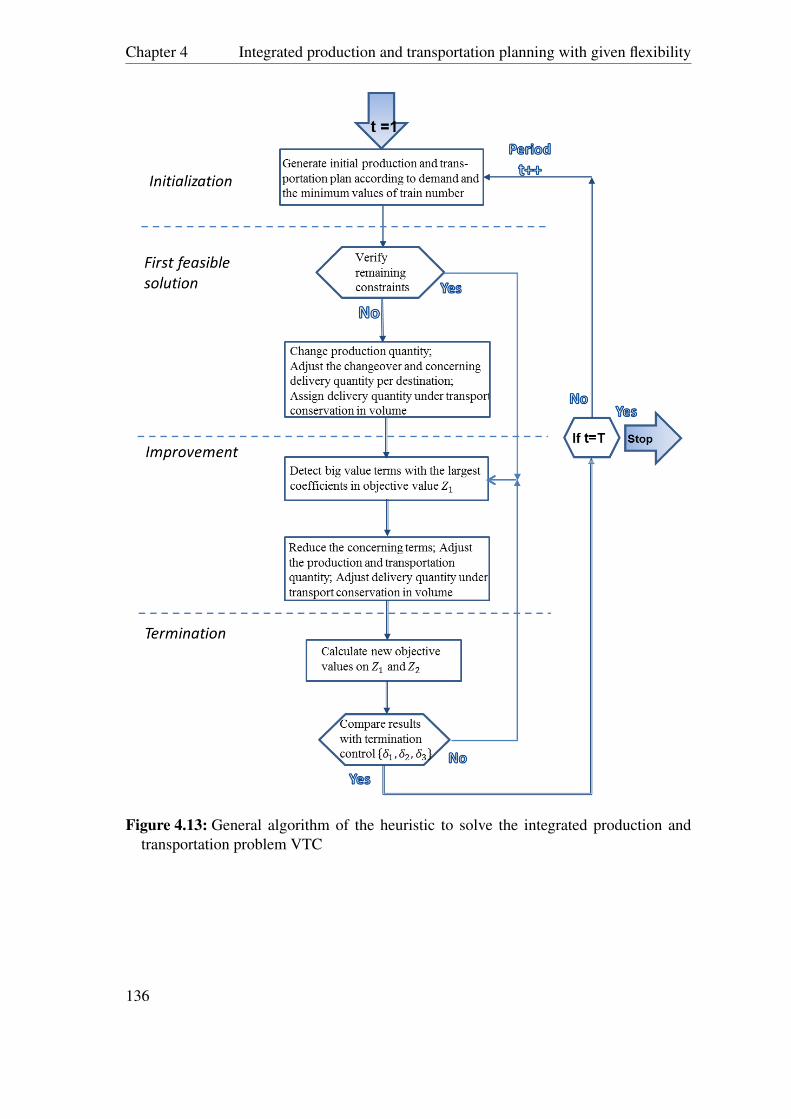
Chapter 4 Integrated production and transportation planning with given flexibility
Figure 4.13: General algorithm of the heuristic to solve the integrated production andtransportation problem VTC
136
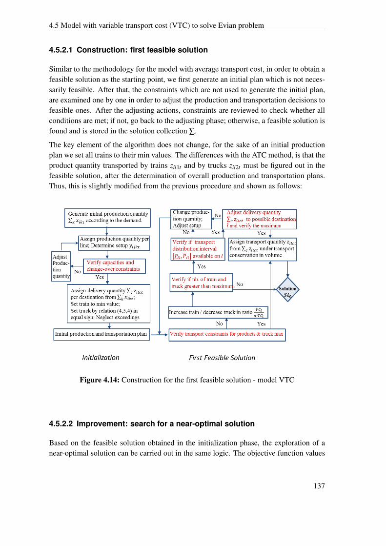
4.5 Model with variable transport cost (VTC) to solve Evian problem
4.5.2.1 Construction: first feasible solution
Similar to the methodology for the model with average transport cost, in order to obtain afeasible solution as the starting point, we first generate an initial plan which is not neces-sarily feasible. After that, the constraints which are not used to generate the initial plan,are examined one by one in order to adjust the production and transportation decisions tofeasible ones. After the adjusting actions, constraints are reviewed to check whether allconditions are met; if not, go back to the adjusting phase; otherwise, a feasible solution isfound and is stored in the solution collection ∑.
The key element of the algorithm does not change, for the sake of an initial productionplan we set all trains to their min values. The differences with the ATC method, is that theproduct quantity transported by trains zil1t and by trucks zil2t must be figured out in thefeasible solution, after the determination of overall production and transportation plans.Thus, this is slightly modified from the previous procedure and shown as follows:
Figure 4.14: Construction for the first feasible solution - model VTC
4.5.2.2 Improvement: search for a near-optimal solution
Based on the feasible solution obtained in the initialization phase, the exploration of anear-optimal solution can be carried out in the same logic. The objective function values
137

Chapter 4 Integrated production and transportation planning with given flexibility
Z1 in Eq. (4.5.1) and Z2 in Eq. (4.5.2) play important roles, since the algorithm detectsvariables of big value with the largest coefficients in objective value Z1 to reduce the totalcost among terms A, B, C, D, E and F for six main costs. The terms E and F are additionalto the the model ATC.
Cost terms A, B, C, D, E and F are presented in detail in the logic bloc, illustrated inFig.4.15 with cases A, B and C, continued in Fig.4.16 with D, E and F. And there is asmall Bloc P’ illustrated in Fig.4.17. If the algorithm comes up to “Bloc P”’ on the left ofFig.4.10, or on the bottom of Fig.4.11 (“Bloc P’ in Case A”), the algorithm enters directlythe small algorithm Bloc P’ for further computation.
From the detailed algorithms in the following, we see the logic of this algorithm hasa similarity to the previous one of model with average transport cost. Because of theintroduction of new parameters and variables to this model, differences between the newheuristic for model VTC and the old one for model ATC, lie principally in the assignmentof transportation quantity zilct by train and by truck of their total one ∑
czilct . Thus, the
linkage between the detailed delivery quantity by train zil1t and by truck zil2t play animportant role.
The case E and case F in Fig.4.16 treat this linkage problem, which is absent in the modelATC. Subsequent operations are simple, in case A, B, C and D, the on-going algorithmmust specify the delivery quantities before and after the transport rearrangement. Somedifferences also lie in the treatment of transport conservation in volume of train and truck,linked by relation (4.5.4), (4.5.8) and (4.5.9), and treated in the algorithm. At the sametime, the problem’s data characteristics are exploited to speed up the algorithm.
138

4.5 Model with variable transport cost (VTC) to solve Evian problem
Figure 4.15: Improvement for the next feasible solution for model VTC - part I
139
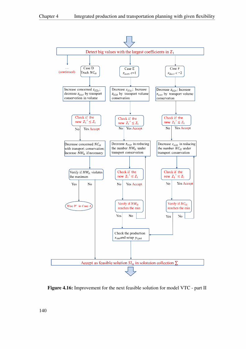
Chapter 4 Integrated production and transportation planning with given flexibility
Figure 4.16: Improvement for the next feasible solution for model VTC - part II
140

4.5 Model with variable transport cost (VTC) to solve Evian problem
Figure 4.17: Improvement for next feasible solution for model VTC - Bloc P’
4.5.2.3 Termination: accept a near-optimal solution and terminate theexploration
All these blocs assure the algorithm to move on between adjacent feasible solutions, andthe exploration of new feasible solution must be terminated using the termination parame-ters N1 and δ1,δ2,δ3 in the same steps in sec.4.4.2.3, in order to provide a near-optimalsolution. As a result, different δ1,δ2,δ3 sets may lead to divers speed of convergenceand different quality of final solutions. The judgement phase of termination remains thesame to the previous bloc for model ATC, so it is omitted to be presented here.
4.5.3 Computational Results
Same to the test in sec.4.4, the computation is performed using a Dell Optiplex 780 com-puter with an Inter Core Duo 2.66 GHz Processor and 3.21 Go RAM under 32 bit Win-dowsXP environment. The proposed heuristic algorithm for the linear problem is codedin language VB2005 (VB.net) with original data provided by the company in Excel files.The Cplex used is Ilog Cplex 11.1 version.
141

Chapter 4 Integrated production and transportation planning with given flexibility
To launch the computation, the truck 44T with 44m3 is adopted by us as default truck andthe wagon with 34 Euro pallets (size 800x1200 m) of volume 120m3 as default wagontype in the train. As described in section sec.4.3, the industrial results are presented inproduction plan and transportation plan in forms of Tab.4.5 and Tab.4.6.
Transportation data is available for the considered periods in 2011 provided by Evian,thus, we propose to compare the transportation plans in Tab.4.11 and Tab.4.6. These areextract tables of our output transportation plan, with 13 transport destinations listed in theleft column and 9 periods for other columns. Train numbers are presented in 9 periodsfor 13 destinations for model VTC. On the bottom of Tab.4.11, the total used trucks arespecified in each period. Truck results of current model VTC is colored in blue, those ofmodel ATC (the previous model) colored in black and those of Evian in red.
Table 4.11: Output transportation plan for Evian problem - comparisonwith model VTC
Significant differences are exposed between output transportation plans of model ATCand model VTC. For instance, 13.5 trains go the direction to Amberieu and 2 trains areheading for Arles/Miramas in period T1, while those numbers of model ATC are respec-tively 14 and 1. At the same time, only 87 trucks are deployed by model ATC, and 95trucks used and sent by model VTC, which is relatively higher. In other periods, mosttruck numbers of model VTC are smaller than those of model ATC. Since the modelVTC give more precision on transportation planning with fixed charge and variable costfor both trains and trucks, the current planning are to provide precised results to achievebetter near-optimal objective value in model VTC. However, the transport differences be-tween VTC and Evian are quite clear, our results send a lot fewer trucks and do not showdrastic increase and decrease. Output transportation plan shows that model VTC have
142

4.5 Model with variable transport cost (VTC) to solve Evian problem
better arranged the train plan with respects to the min-max interval in periods, which isresult of the proposed heuristic. In this way, the comparison between transportation plansconfirms that our approach works efficiently to provide good integrated production andtransportation plans.
Still, tests are carried out to compare solution qualities and computation times with threealgorithms. The suggested problem-specific heuristic presented in this previous sub-section is the first one, with two sets of control thresholds δ = δ1,δ2,δ3 in δ 1 =
6%,90%,0.02% and δ 2 = 3%,95%,0.005%. The second algorithm uses the mixedinteger optimizer in ILOG CPLEX, where two level objectives are merged into a singleobjective function by weighting the objective Z1 200 times than Z2, using the traditionalbranch-and-bound technique to obtain an optimal solution if we could wait until termina-tion.
The third algorithm is the heuristic-CPLEX combined method, introducing the initialfeasible solution generated by the suggested heuristic as the starting point of CPLEXprogram and afterwards, searching for the optimal solution in the traditional branch-and-bound way.
Table 4.12: Comparison on objective value and run time with three algorithmsin Model VTC
Tab.4.12 shows the comparison on objective value and computation time for the threealgorithms. The first column marks the scenario datasets: for set SKU50, where the inputscenario consists of only 50 SKUs on 3 production lines for 4 warehouse destinations in12 weeks; 100 SKUs on 6 lines to 5 warehouses for SKU100 in 12 weeks; 200 SKUson 7 lines to 8 warehouses for SKU200; 420 SKUs on 14 lines to 14 warehouses. Forheuristic column, the results are listed in termination criterion δ 1 = 6%,90%,0.02%and δ 2 = 3%,95%,0.005%, presented in the sec.4.4.2.3. For objective value column,Z1 is the total cost in euro and for time column in CPU seconds.
We would conclude that the CPLEX optimizer provides always the best solution by look-ing for an optimal solution, and at the same time, it consumes enormous amount of com-putational time because of a large amount of integer variables. We observe this time, for
143

Chapter 4 Integrated production and transportation planning with given flexibility
the set SKU420, CPLEX cannot achieve the optimal solution in a reasonable amount oftime, while in the results for model ATC, set SKU420 is still passable. The introduc-tion of new variables and new constraints increase the complexity of the problem, andthe CPLEX optimizer manifest worse performance in time-consuming. In contrary, thesuggested heuristic is observed to provide a good approximate solution in 132 seconds,that means just a few minutes are enough to complete computing for set SKU420, whileCPLEX optimizer encounters difficulties to look for the next feasible solution. Thus, theproposed heuristic has significantly sped up the solution exploration. It is also noticeablethat the results with termination control δ 1compute more speedily than δ 2, while δ 2 couldprovide better solution.
Besides, the total cost value Z1 in model VTC is generally bigger in each set than thatof model ATC, due to transport cost data in more precision. The Gap in the last columnindicates the relative error of the heuristic solutions against the optimal solutions fromCPLEX program, while the termination δ 1 shows bigger errors than δ 2. For the twotermination groups, all the Gap values are greater that those in the model ATC, mainlydue to increased complexity from new variables and new constraints. We can see clearlyin the table, the Gap increases as the problem size increases. However, the Gap valuesobserved are not remarkable: for termination δ 1, they are increased but still kept around0.1% for the SKU200; for termination δ 2, kept tiny below 0.05%. The performance ofthe proposed heuristic to seek solutions with good quality is well preserved.
In the last column of Tab.4.12, the combined method with heuristic feasible solution andCPLEX MIP program turns out with less consuming time when providing a solution withsimilar quality to that obtained with the unique CPLEX optimizer. This result is similarto that described in section sec.4.4 of model ATC. The results of the model VTC prove aswell that the combined method works pretty quicker than the unique traditional branch-and-bound method. Thus, for a relatively small size problem with less integer variables,the combined method may be a good alternative compared to the traditional branch-and-bound CPLEX program. For a synchronized planning problem over 12 weeks updatedeach week with tremendous integer variables in industrial case, it is unpractical to lookfor a guaranteed optimal solution in waiting for such long time. In this way, the proposedproblem-specific heuristic works efficiently, and the results issued in a few minutes arewell within the range of tractability.
144

4.6 Conclusion
4.6 Conclusion
Flexibility considerations lie in every step of the supply chain, where the production andtransportation activities count for large costs. Literature on production planning problems,transportation planning problems and integrated production and transportation planningproblems in supply chain are reviewed and discussed in the first half part of this chapter.
At the second half of the chapter, we take a glance at a real life production and transporta-tion system, and attempt to exploit its given flexibility tolerances in an optimized way.The company has many restrictions on its production and transportation planning, such asno storage space and limited available train numbers, whereas some other allowable flex-ibility intervals are imposed to its planning system, like flexible distribution percentagesto this or that warehouses. All these requirements lead to a conclusion that its productionplanning and transportation operations need to be integrated and optimized in a synchro-nizing way. In fact, three heterogeneous modes of transportation appear in this study: (i)railway train, (ii) truck, (iii) multi-modal transport with train plus truck. Moreover, sinceeach train is composed of different numbers of wagon, and a wagon contains differentnumbers of pallet, the transportation mode is more heterogeneous than a great part ofstudies in the literature.
The industrial problem is then formulated as a mixed integer programming problem con-sidering an Average Transportation Cost (ATC) for unit products by train and by trucks tosimplify the model, and then solved by a problem-specific heuristic procedure. Comparedwith the traditional CPLEX program, the heuristic combined CPLEX method can providean optimal solution in consuming less computation time, and the proposed heuristic cangive a good near-optimal solution in a considerably less time. The gap between our so-lutions against those by CPLEX program are pretty insignificant, for some terminationcriterion, the gap away from the optimal solution remains quite tiny (<0.05%).
Furthermore, in order to obtain more details, we slightly modify the first model with Aver-age Transport Cost (ATC) per pallet by train and by truck, and then the triple subscripteddecision variables in the model ATC become quadruple, called model with Variable Trans-port Cost (VTC). Products coded with different references can be easily transported to-gether in a same train wagon or a truck. A same logic problem-specific heuristic coding inVB.Net is proposed to solve the problem, and compared again with the CPLEX solutionand the combined heuristic-CPLEX solution. The results prove that the combined methodruns more quickly than the unique traditional branch-and-bound method and gives an op-timal solution if the number of variables is reasonable. Therefore, the combined methodmay be a good alternative compared with the traditional branch-and-bound method if thedecision variables quantity are not too immense. Whereas in our case, for an integratedproduction and transportation planning problem over 12 weeks updated with tremendousinteger variables, it is unpractical to wait such long time for a guaranteed optimal solu-
145

Chapter 4 Integrated production and transportation planning with given flexibility
tion. In this way, the proposed problem-specific heuristic works efficiently to give a goodnear-optimal solution within a reasonable amount of computation time.
146

5 Conclusions and future researchdirections
Conclusions
Supply chain strategies have evolved considerably in recent decades. Under the increasingcompetition in the global market, a good adoption and integration of flexibility decisionscan reduce considerably the supply chain operating costs and lead to better potential com-petitiveness.
The first objective of the work is to provide a better understanding of supply chain flex-ibility. For the time being, there is no taxonomy of supply chain flexibility universallyaccepted in the literature and in industries. We first describe different conceptual aspectsof flexibility existing in the literature and causative uncertainties. Interconnections andoverlappings among flexibility dimensions are revealed and exhibited, as well as the pre-sentation of flexibility terms which are more frequently supported in the literature or ofgreat importance. The flexibility concepts from the supplier, manufacturer, distributor andalso all the three are integrated as a whole. In this way, a new framework of supply chainflexibility is outlined and proposed, with several flexibility terms called major flexibilitiesand other flexibilities. This new flexibility framework is based on 8 core dimensions: ma-chine, labor, routing, product-mix, volume, supplier, delivery and transshipment flexibil-ity. This framework provides a clear definition and classification, and leads to a completeunderstanding of the supply chain flexibility. Moreover, we clarify the levers that serveas an action to influence corresponding flexibilities to enrich this framework, which is ofgreat practical sense for companies to set about on how to implement the flexibility in theindustry. This chapter 2 has contributed for the defining phase of supply chain flexibility.
In the following part of work, we review the existing evaluation methodologies of supplychain flexibility, and are aware that quantitative studies are still not extensive. Method ofRogalski [Rog11] incorporating explicitly the volume flexibility, product-mix flexibilityand expansion flexibility, is carefully presented because each of them can be expressedseparately without interfering too much into the analytical model for details. Other mea-sures and methods as Penalty of Change, Design of Systems for Manufacture, Mechanical
147

Chapter 5 Conclusions and future research directions
Analogy, Simulation of Petri nets and Toolbox Approach are reviewed. To settle an prac-tical assessment on hand, we implement Mechanical Analogy method in supply chain toevaluate the flexibility performance for stores of Louis Vuitton in Japan. This methodwas rough and never used in supply chain, and our study extends its application scopeto whole supply chain and provide good understandable results. We then conclude that,the flexibility performance of one store is generally lower and not as stable as the biggerstores during a year, whereas the products in bigger volume manifest a general better flex-ibility throughout the year. These results coincide with the real situation of the company,and can help the company identify the flexibility behavior of its stores and products. Asa result, a practical evaluation procedure is established to carry out this method in supplychain, where the notion of period-classification and object-classification are emphasizedbefore implementing the analogy method.
We also review the literature on traditional production planning problems, traditionaltransportation planning problems and then the integrated production and transportationproblems. To go further, we go inside an integrated planning problem, especially with aset of given flexibilities. In the Evian situation, no storage space is placed on site, whichimplies a strong interference between activities of production and transportation. The ex-istence of heterogeneous vehicles is emphasized and presented by train and by truck, andwe underline the detailed choice that each train can be fractionated to different numbersof wagon, and a wagon contain different numbers of different pallets. As a result, thetransportation mode in this model is more heterogeneous than a great part of studies inthe literature.
To solve this problem efficiently, we formulate two mixed integer programs, the firstmodel with an average transportation cost, the other with fixed and variable transportationcost. The solutions are both obtained by three algorithms: the proposed problem-specificheuristics, the traditional branch-and-bound in CPLEX program, and the heuristics-CPLEXcombined method. Results prove that the near-optimal solution of our heuristics is closeto the optimal one by CPLEX, and runs within a considerably less amount of computa-tion time. Even the CPLEX combined method works quicker than the unique traditionalbranch-and-bound one. In this way, the proposed problem-specific heuristic is proved tobe efficient in solving the Evian problem, and the results issued in a few minutes comparedwith the optimal solution are well within satisfiable quality. Furthermore, the CPLEXcombined method is proved to be really a good approach to look for an optimal solutionin considerably less amount of time, if the quantity of decision variables is not too large.
In conclusion, our thesis has well worked to contribute to fill in traditional gaps betweenacademic research and industrial needs mainly on three flexibility fields: i) defining thesupply chain flexibility; ii) assessing the supply chain flexibility; and iii) use and manage-ment on supply chain flexibility.
148
Conclusions and future research directions
Future research directions
For the time to date, quantitative researches on supply chain flexibility are increasinglyblooming but still limited. More quantitative methods need to be explored, with theknowledge that a general applicable methodology for different business sectors is difficultto construct. Particularly, methodologies that develop and evaluate a specific subdividedflexibility - the precise dimension of flexibility - are relatively few but extensively inter-esting for industries. Therefore, it would be quite a good direction to raise further studies.
In the mechanical analogy method, several attributes remain hidden behind the analogicalsystem and can be further investigated. Firstly, a mechanical system of a single degree offreedom has always an elastic spring, a damper and a mass. It is simple to derive a math-ematical relation on analogical mass of a supply chain, but difficult to acquire a detailedpresentation of the corresponding spring and damper. Therefore, a further direction forthis method is to develop this relation to describe a meaningful and representable stiff-ness and damper of the studied supply chain, which is important to understand the threeanalogical system attributes. And if impossible to go on in this way, one can adopt thesimulation approach to observe: with different input and output data, what has exactlyhappened in the interior of the company? In this manner, although it is hard to obtain aprecise formulation of stiffness and damper of supply chain, an approximate relation tounderstand the supply chain’s mechanical properties would be possible.
Another research point is, if the degree of freedom of a supply chain or a sub-echelon of asupply chain can be identified, the exact mechanical analogy can be made, in analogy to avibration system with more than one degree of freedom. For a vibrator system with morethan one mass, spring or damper in successive way or in parallel, the corresponding supplychain may manifest similar behavior. The limit lies in the fact that, this kind of mechanicalsystem is difficult to be studied, because the analogical response is complicated to beformulated with much more deres of freedom, but remains a really interesting researchdirection.
For the integrated production and transportation planning problems, flexibility tolerancesare always severe questions. More integrated planning models with given flexibility in-tervals can be developed, and some particular measures presented in chapter 3 could beincorporated in the model.
Nevertheless, the existing integrated production and transportation planning studies havelittle explored heterogeneous transportation modes. For instance, there are three hetero-geneous modes of transportation in our study in sec.4.3: (i) railway train, (ii) truck, (iii)multi-modal transport with train plus truck. As an example, this could be further devel-oped with more complex delivery modes in the following : (i) railway train with integratedproduction and transportation option, (ii) truck with non integrated production and trans-
149
Chapter 5 Conclusions and future research directions
portation planning options, (iii) multi-modal transportation with partial integration, etc.Thus, heterogeneous transportation usage can be further explored.
Most existing studies on integrated production and transportation planning consider de-terministic models where product demand is known in advance. However, many kinds ofproducts in real world does not figure in this field. For example, for products having alarge variety with short life cycle, the customer demand is of high uncertainty and diffi-cult to anticipate. Furthermore, most existing production-transportation problems involvelinear transportation costs, which may be unrealistic in industry. Therefore, more furtherstudies with nonlinear cost and stochastic demand are expected.
Additionally, for the integrated production and transportation planning problems solvedby the traditional branch-and-bound CPLEX program and the heuristics-CPLEX com-bined method, the latter provides optimal solutions within a pretty quicker computationtime. It is the method to obtain a first feasible solution by our proposed efficient heuris-tics, and then use this feasible solution as the starting point of CPLEX program. Thismethod demonstrates a pretty better performance in computation time, and worth to beimplemented to reduce the running time in solving other complex problems if the datascale is not too tremendous.
150

Annex I - Transportation planningproblem
A simple form of multi-plant, multi-commodity, multi-DC, multi-customer and two-echelontransportation problem at tactical level could be formulated as follows:
Decision Variablesxi jkm quantity of commodity i to be shipped from plant j through
distribution center k to customer market zone mykm binary variable will be 1 if DC k serves the customer zone m,
otherwise 0zk binary variable will be 1 if DC k is acquired and opened, otherwise 0
ParametersDim demand of commodity i in customer market zone mSi j supply of commodity i at plant jV k,V k allowed minimum and maximum annual throughput for a DC kcdk fixed annual possession and operation cost for DC kcvk variable cost per unit for DC kcti jkm transportation cost per unit for shipping commodity i from plant j
through DC k to customer market zone mtikm average time to make a delivery for commodity i to zone m after
receiving an order at DC kTi maximum allowed delay of commodity i
The objective function is formulated:
Min : Z = ∑i∑
j∑k∑m
cti jkm · xi jkm +∑k
(cdk · zk + cvk ·∑
i∑m
ykm ·Dim
)(.0.1)
subject to
151

Annex
∑j
xi jkm = ykm ·Dim ∀i, ∀k, ∀m (.0.2)
∑k∑m
xi jkm ≤ Si j ∀i, ∀ j (.0.3)
V k·zk ≤∑i∑m
ykm ·Dim ≤V k · zk ∀k (.0.4)
(∑k∑m
tikm · ykm ·Dim
)≤ Ti ·∑
mDim ∀i (.0.5)
ykm = 0,1 , zk = 0,1 ∀k, ∀m (.0.6)
xi jkm ≥ 0 ∀i, ∀ j, ∀k, ∀m (.0.7)
In this formulation, the amount ∑i∑m
ykm ·Dim interprets the total annual throughput of the
distribution center k. Constraints (.0.2) specify the flow conversation for customer marketdemand and also xi jkm must be 0 for all i, j if ykm = 0. Constraints (.0.3) insure the sup-ply quantity of commodity i. Constraints (.0.4) stipulate the correct logical relationshipbetween binary variable ykm and zk and make sure the total annual throughput lies in theright interval. Constraints (.0.5) keep the order lead time less or equal than the maximumdelay to customers.
From this formulation, a market zone m can be served simultaneously by several distri-bution centers. If it is not the case, we can still add a relation (.0.8) to restrict a certainmarket zone m = l to be served by a single DC:
∑k
ykl = 1 ∀l (.0.8)
152
Acknowledgments
The cost term cti jkm can be also modified into a cost function containing a fixed chargeand a variable part. In the case that some commodities must be shipped and delivereddirectly from plants to customers, terms of corresponding cost cti jkm could be definedindependent of intermediate DC, and the corresponding combinations for commodity iand market zone m could be omitted in the term ∑
i∑m
ykmDim. If a certain market zone is
supposed to receive all commodities directly from its plant, a fictitious distribution centerk0 could be added, together with the associated zk0 , yk0m and cti jk0m in the model.
153


Annex II - Integrated Production andtransportation problems class (A)
This model is a simple integrated production-transportation, facility location-allocationproblem [PF2] in problems class (A) described in sec.4.2.3.1.
For a typical production-transportation, facility location-allocation problem across mul-tiple stages of the supply chain, decision variables and parameters in different echelonsmust be taken into account. Consider a simple multi-supplier, multi-plant, multi-level,multi-commodity, single-period and homogeneous vehicle problem, on condition that awarehouse serves only one customer zone, we list all the decision variables and parame-ters as follows:
Decision Variablesxlk production quantity of product l produced at plant kqi jkl quantity of product l shipped from plant k via warehouses j to
customer zone imskr quantity of raw material r shipped from supplier s via warehouses to
plant kpk binary variable 0,1 indicating whether the plant k is open or notyi j binary variable 0,1 indicating whether the warehouse j serves
customer zone i or notz j binary variable 0,1 indicating whether the warehouse j is open or
not
Input dataow j annual fixed cost for operating a warehouse at site jopk annual fixed cost for operating a plant kvw j unit cost of throughput for a warehouse at site jvplk unit production cost for product l at plant ktsskr unit transportation and purchasing cost from supplier s to plant k for
raw material r
155

Annex
Input data (continued)twi jkl unit transportation cost for product l from plant k via warehouse j to
customer zone idil demand for product l at customer zone iWj annual throughput at warehouse jCk capacity of plant kCSsr supply capacity of supper s for raw material rurl utilization rate of raw material r per unit of finished product lCul capacity utilization rate per unit of finished product lP maximum opened facilitiesW maximum opened warehouses
The problem can be then formulated as a cost-based minimization model:
[PF2] Min : Z = ∑j
ow jz j +∑i∑
j∑
lvw jdilyi j +∑
kopk pk
+∑l∑k
vplkxlk +∑s∑k∑r
tsskrmskr (.0.9)
+∑i∑
j∑k∑
ltwi jklqi jkl
subject to
∑j
yi j = 1 ∀i (.0.10)
∑i∑
ldilyi j ≤Wjz j ∀ j (.0.11)
∑j
z j ≤W (.0.12)
∑k
qi jkl = dilyi j ∀i, ∀ j, ∀l (.0.13)
156

Acknowledgments
∑k
mskr ≤CSsr ∀s, ∀r (.0.14)
∑l
urlxlk ≤∑s
mskr ∀k, ∀r (.0.15)
∑l
Culxlk ≤Ck pk ∀k (.0.16)
∑i∑
jqi jkl ≤ xlk ∀l, ∀k (.0.17)
∑k
pk ≤ P (.0.18)
zi, pk, yi j = 0, 1 ∀i, ∀ j, ∀k (.0.19)
mskr, xlk, qi jkl ≥ 0 ∀i, ∀ j, ∀k, ∀s, ∀r (.0.20)
The objective function (.0.9) minimizes the total cost, including the fixed cost of open-ing and operating plants and warehouses, the variable cost of production and distribution,transportation cost to transfer raw materials from suppliers to plants and to transfer fin-ished products from plants to retailers through warehouses. Constraint (.0.10) shows thesimple assignment of a warehouse to a customer zone and the warehouse throughput isimposed by (.0.11). Constraints (.0.12) and (.0.18) limit the total number of openingwarehouses and plants. Constraint (.0.13) ensure that each demand is satisfied withoutbacklogging. Raw material restriction and requirement for production are expressed in(.0.14) and (.0.15). Production in the plants is subject to capacity constraint (.0.16). Foreach product, the total quantity shipped from one plant to all customer zones throughwarehouses cannot exceed the production quantity of that product in this plant in (.0.17).
157
Annex
Finally, constraint (.0.19) and constraint (.0.20) impose the integrality restriction and non-negativity condition on the decision variables.
The problem formulation [PF2] can be easily extended to multi-period model with inven-tory flow conservations backlogged or not, between any two adjacent periods. Warehouseassignment in constraint (.0.10) can be modified for the sake of serving more customeroutlets. In order to take heterogeneous vehicles into account, the unit transportation andpurchasing cost, noted as tsskr, with indices from supplier s to plant k for raw material r,can be splitted into multiple costs tsskrv with different vehicles v = 1, 2, ...,V , if the costsare vehicle-independent. Meanwhile, the unit transportation cost designated by twi jkl , forproduct l from plant k via warehouse j to customer zone i, can be transformed in the sameway: twi jklv for independent vehicle modes v = 1, 2, ...,V . On condition that the vehi-cle utilization cost is dependent one to another, tsskr and twi jkl are forced to be functionsof the existing vehicle modes tsskr = tsskr(v1,v2, ...,vV ) and twi jkl = twi jkl(v1,v2, ...,vV ).And, the vehicle velocity, volume and loading limits could be also studied for a moredetailed problem construction.
158

Reference
[AA06] H. Allaoui and A. Artiba. Scheduling two-stage hybrid flow shop withavailability constraints. Computers & Operations Research, 33(5):1399–1419, 2006.
[AA14] H. Allaoui and A. Artiba. Hybrid flow shop scheduling with availabilityconstraints. In Essays in Production, Project Planning and Scheduling,pages 277–299. Springer, 2014.
[AADRR09] K. Antony Arokia Durai Raj and C. Rajendran. Fast heuristic algorithmsto solve a single-stage fixed-charge transportation problem. InternationalJournal of Operational Research, 6(3):304–329, 2009.
[AADRR12] K. Antony Arokia Durai Raj and C. Rajendran. A genetic algorithm forsolving the fixed-charge transportation model: Two-stage problem. Com-puters & Operations Research, 39(9):2016–2032, September 2012.
[AB91] B. R. Allen and A. C. Boynton. Information architecture: in search ofefficient flexibility. MIS quarterly, 15(4):435–445, 1991.
[Adl88] P. S. Adler. Managing flexible automation. California Management Review,30(3):34–56, 1988.
[AGL08] R. Armstrong, S. Gao, and L. Lei. A zero-inventory production and dis-tribution problem with a fixed customer sequence. Annals of OperationsResearch, 159(1):395–414, 2008.
[AK99] V. Adlakha and K. Kowalski. On the fixed-charge transportation problem.Omega, 27(3):381–388, 1999.
[AKVL07] V. Adlakha, K. Kowalski, R. R. Vemuganti, and B. Lev. More-for-lessalgorithm for fixed-charge transportation problems. Omega, 35(1):116–127, 2007.
[AM05] E. D. Arnheiter and J. Maleyeff. The integration of lean management andsix sigma. The TQM magazine, 17(1):5–18, 2005.
[AMMC05] K. Alexopoulos, A. Mamassioulas, D. Mourtzis, and G. Chryssolouris. Vol-ume and product flexibility: a case study for a refrigerators producing fa-cility. In Proceedings of 10th IEEE Conference on Emerging Technologiesand Factory Automation, pages 891–897, Catania, Italy, 2005.
159

Reference
[AMPC07] K. Alexopoulos, D. Mourtzis, N. Papakostas, and G. Chryssolouris.Desyma: assessing flexibility for the lifecycle of manufacturing systems.International Journal of Production Research, 45(7):1683–1694, 2007.
[AP93] A. Aggarwal and J. K. Park. Improved algorithms for economic lot sizeproblems. Operations Research, 41(3):549–571, 1993.
[APK+95] D. E. Avison, P. L. Powell, P. Keen, J. H. Klein, and S. Ward. Addressingthe need for flexibility in information systems. Journal of ManagementSystems, 7(2):43–60, 1995.
[APM+07] K. Alexopoulos, N. Papakostas, D. Mourtzis, P. Gogos, and G. Chrys-solouris. Quantifying the flexibility of a manufacturing system by applyingthe transfer function. International Journal of Computer Integrated Manu-facturing, 20(6):538–547, September 2007.
[APM+08] K. Alexopoulos, N. Papakostas, D. Mourtzis, P. Gogos, and G. Chrys-solouris. Oscillator analogy for modelling the manufacturing systems dy-namics. International Journal of Production Research, 46(10):2547–2563,2008.
[Arv05] S. Arvanitis. Modes of labor flexibility at firm level: Are there any impli-cations for performance and innovation? evidence for the swiss economy.Industrial and Corporate Change, 14(6):993–1016, 2005.
[Bad99] M. A. Badri. Combining the analytic hierarchy process and goal program-ming for global facility location-allocation problem. International Journalof Production Economics, 62(3):237–248, September 1999.
[Bal61] M. L. Balinski. Fixed-cost transportation problems. Naval Research Logis-tics Quarterly, 8(1):41–54, 1961.
[Bay09] A. Baykasoglu. Quantifying machine flexibility. International Journal ofProduction Research, 47(15):4109–4123, 2009.
[BCFS13] Z. Benchemsi, P.-Y. Champagne, R. Fraysse, and A. Samar. Flexibilitéde la partie aval de la supply chain. Project report, Ecole Cenrale Paris,Department of Industrial Engineering, 06 2013.
[BDR+84] J. Browne, D. Dubois, K. Rathmill, S. P. Sethi, and K. E. Stecke. Classifica-tion of flexible manufacturing systems. The FMS magazine, 2(2):114–117,1984.
[BE03] M. Barad and D. Even Sapir. Flexibility in logistic systems-modeling andperformance evaluation. International Journal of Production Economics,85(2):155–170, August 2003.
160

Reference
[Ber03] J. W. M. Bertrand. Supply chain design: flexibility considerations. InHandbooks in Operations Research and Management Science, volume 11,pages 133–198. Elsevier, 2003.
[BF12] A. Boloori Arabani and R. Z. Farahani. Facility location dynamics: Anoverview of classifications and applications. Computers & Industrial Engi-neering, 62(1):408–420, 2012.
[BJ10] A. N. Balaji and N. Jawahar. A simulated annealing algorithm for a two-stage fixed charge distribution problem of a supply chain. InternationalJournal of Operational Research, 7(2):192–215, 2010.
[Ble04] K. Bleicher. Das konzept integriertes management: Visionen–missionen–programme, 7. überarbeitete und erweiterte auflage. Frankfurt am Main,2004.
[BMP+00] R. Beach, A. P. Muhlemann, D. H. R. Price, A. Paterson, and J. A. Sharp.A review of manufacturing flexibility. European Journal of OperationalResearch, 122(1):41–57, 2000.
[BO04] B. Bilgen and I. Ozkarahan. Strategic tactical and operational production-distribution models: a review. International Journal of Technology Man-agement, 28(2):151–171, 2004.
[Boy10] N. Boysen. Truck scheduling at zero-inventory cross docking terminals.Computers and Operation Research, 37(1):32–41, 2010.
[BS88] M. Barad and D. Sipper. Flexibility in manufacturing systems: definitionsand petri net modelling. The International Journal Of Production Research,26(2):237–248, 1988.
[BVRW84] I. Barany, T. J Van Roy, and L. A. Wolsey. Strong formulations for multi-item capacitated lot sizing. Management Science, 30(10):1255–1261, 1984.
[BY82] G. R. Bitran and H. H. Yanasse. Computational complexity of the capaci-tated lot size problem. Management Science, 28(10):1174–1186, 1982.
[CBW07] F. T. S. Chan, R. Bhagwat, and S. Wadhwa. Flexibility performance:Taguchi’s method study of physical system and operating control param-eters of fms. Robotics and Computer-Integrated Manufacturing, 23(1):25–37, 2007.
[CC07] F. Chu and C. Chu. Polynomial algorithms for single-item lot-sizing mod-els with bounded inventory and backlogging or outsourcing. IEEE Trans-actions on Automation Science and Engineering, 4(2):233–251, 2007.
[CC08] F. Chu and C. Chu. Single-item dynamic lot-sizing models with boundedinventory and out-sourcing. IEEE Transactions on Systems, Man and Cy-bernetics Part A: Systems and Humans, 38(1):1–8, 2008.
161
Reference
[CC10] H. K. Chan and F. T. S. Chan. Comparative study of adaptability and flex-ibility in distributed manufacturing supply chains. Decision Support Sys-tems, 48(2):331–341, January 2010.
[CCTZ10] M. C. Chou, G. A. Chua, C.-P. Teo, and H. Zheng. Design for processflexibility: Efficiency of the long chain and sparse structure. OperationsResearch, 58(1):43–58, March 2010.
[CCZ+12] C. Chu, F. Chu, M. C. Zhou, H. Chen, and Q. Shen. A polynomial dy-namic programming algorithm for crude oil transportation planning. IEEETransactions on Automation Science and Engineering, 9(1):42–55, 2012.
[CCZY13] C. Chu, F. Chu, J. Zhong, and S. Yang. A polynomial algorithm for a lot-sizing problem with backlogging, outsourcing and limited inventory. Com-puters & Industrial Engineering, 64:200–210, 2013.
[CF94] P. Chandra and M. L. Fisher. Coordination of production and distribu-tion planning. European Journal of Operational Research, 72(3):503–517,1994.
[CGM05] R. L. Cook, B. J. Gibson, and D. MacCurdy. A lean approach to crossdocking. Supply Chain Management, 9:54–59, 2005.
[CH05] J.-H. Chen and S.-Y. Ho. A novel approach to production planning of flex-ible manufacturing systems using an efficient multi-objective genetic al-gorithm. International Journal of Machine Tools and Manufacture, 45(7-8):949–957, June 2005.
[Che96] Z.-L. Chen. Scheduling and common due date assignment with earliness-tardiness penalties and batch delivery costs. European Journal of Opera-tional Research, 93(1):49–60, August 1996.
[Che97] J. Chen. Achieving maximum supply chain efficiency. IEE Solutions,June:30–35, 1997.
[Che10] Z.-L. Chen. Integrated production and outbound distribution scheduling:review and extensions. Operations Research, 58(1):130–148, 2010.
[Chr96] G. Chryssolouris. Flexibility and its measurement. CIRP Annals-Manufacturing Technology, 45(2):581–587, 1996.
[CL88] M. A. Cohen and H. L. Lee. Strategic analysis of integrated production-distribution systems: models and methods. Operations Research,36(2):216–228, 1988.
[CL04] Y.-C. Chang and C.-Y. Lee. Machine scheduling with job delivery coordi-nation. European Journal of Operational Research, 158(2):470–487, 2004.
162

Reference
[Cou02] Supply-Chain Council. Supply chain council, inc. http://www.supply-chain.org/resources/faq.htm, 2002.
[Cox58] E. F. Cox. The metric system: A quarter-century of acceptance (1851-1876). Osiris, pages 358–379, 1958.
[Cox89] T. Cox. Toward the measurement of manufacturing flexibility. Productionand Inventory Management Journal, 30(1):68–72, 1989.
[CP05] Z.-L. Chen and G. Pundoor. Integrating order scheduling with packing anddelivery. Technical report, Robert H. Smith School of Business, Universityof Maryland, College Park, MD 20742, 2005.
[CP06] Z.-L Chen and G. Pundoor. Order assignment and scheduling in a supplychain. Operations Research, 54(3):555–572, 2006.
[CR05] S. Cohen and J. Roussel. Strategic supply chain management: the fivedisciplines for top performance. McGraw-Hill Companies, 2005.
[CT90] W. H. Chen and J. M. Thizy. Analysis of relaxations for the multi-itemcapacitated lot-sizing problem. Annals of operations Research, 26(1):29–72, 1990.
[CW97] M. Chen and W. Wang. A linear programming model for integrated steelproduction and distribution planning. International Journal of Operations& Production Management, 17(6):592–610, 1997.
[Das11] K. Das. Integrating effective flexibility measures into a strategic sup-ply chain planning model. European Journal of Operational Research,211(1):170–183, May 2011.
[DFF01] C. Dhaenens-Flipo and G. Finke. An integrated model for an industrialproduction-distribution problem. IIE Transactions, 33(9):705–715, 2001.
[DG99] K. Dogan and M. Goetschalckx. A primal decomposition method for the in-tegrated design of multi-period production–distribution systems. Iie Trans-actions, 31(11):1027–1036, 1999.
[Dia91] M. Diaby. Successive linear approximation procedure for generalized fixed-charge transportation problems. Journal of the Operational Research Soci-ety, 42(11):991–1001, 1991.
[DMC11] R. Dondo, C. A. Méndez, and J. Cerdá. The multi-echelon vehicle routingproblem with cross docking in supply chain management. Computers &Chemical Engineering, 35(12):3002–3024, 2011.
[DTT01] A. De Toni and S. Tonchia. Performance measurement systems-models,characteristics and measures. International Journal of Operations & Pro-duction Management, 21(1/2):46–71, 2001.
163

Reference
[DVL03] L. K. Duclos, R. J. Vokurka, and R. R. Lummus. A conceptual modelof supply chain flexibility. Industrial Management & Data Systems,103(6):446–456, 2003.
[DW00] D. E. D’Souza and F. P. Williams. Toward a taxonomy of manufacturingflexibility dimensions. Journal of Operations Management, 18(5):577–593,August 2000.
[EEP06] S. D. Eksioglu, H. Edwin Romeijn, and P. M. Pardalos. Cross-facility man-agement of production and transportation planning problem. Computers &Operations Research, 33(11):3231–3251, November 2006.
[EJSD14] Ayse Sena Eruguz, Zied Jemai, Evren Sahin, and Yves Dallery. Optimisingreorder intervals and order-up-to levels in guaranteed service supply chains.International Journal of Production Research, 52(1):149–164, 2014.
[EK00] R. Ernst and B. Kamrad. Evaluation of supply chain structures throughmodularization and postponement. European Journal of Operational Re-search, 124(3):495–510, August 2000.
[EKD10] S. Erhan Kesen, A. Kanchanapiboon, and S. K. Das. Evaluating supplychain flexibility with order quantity constraints and lost sales. InternationalJournal of Production Economics, 126(2):181–188, August 2010.
[EM87] G. D. Eppen and R. K. Martin. Solving multi-item capacitated lot-sizingproblems using variable redefinition. Operations Research, 35(6):832–848,1987.
[ESV06] S. S. Erenguc, N. C. Simpson, and A. J. Vakharia. Integrated produc-tion/distribution planning in supply chains: An invited review. Europeanjournal of operational research, 115(2):219–236, 2006.
[ETAMA12] A. M. El-Tamimi, M. H. Abidi, S. H. Mian, and J. Aalam. Analysis ofperformance measures of flexible manufacturing system. Journal of KingSaud University - Engineering Sciences, 24(2):115–129, July 2012.
[FDMD95] Y. Frein, M. Di Mascolo, and Y. Dallery. On the design of generalizedkanban control systems. International Journal of Operations & ProductionManagement, 15(9):158–184, 1995.
[Fis04] M. L. Fisher. The Lagrangian relaxation method for solving integer pro-gramming problems. Management Science, 50(12 Supplement):1861–1871, December 2004.
[FLM11] D. Francas, N. Löhndorf, and S. Minner. Machine and labor flexibility inmanufacturing networks. International Journal of Production Economics,131(1):165–174, 2011.
164

Reference
[Flo80] M. Florian. Deterministic production planning: Algorithms and complex-ity. Management science, 26(7):669–679, 1980.
[Fra86] E. H. Frazelle. Flexibility: a strategic response in changing times. IndustrialEngineering, 18(3):17–20, 1986.
[Fre06] P. Fredriksson. Cooperation and conflict in modular production and supplierparks: the case of volvo cars’ modular assembly system. Internationaljournal of automotive technology and management, 6(3):298–314, 2006.
[FV99] F. Fumero and C. Vercellis. Synchronized development of production, in-ventory, and distribution schedules. Transportation science, 33(3):330–340, 1999.
[FW81] M. L. Fair and E. W. Williams. Transportation and logistics. BusinessPublications, 1981.
[GAL06] M. Gen, F. Altiparmak, and L. Lin. A genetic algorithm for two-stage trans-portation problem using priority-based encoding. Or Spectrum, 28(3):337–354, 2006.
[GC00] M. Gen and R. Cheng. Genetic algorithms and engineering optimization,volume 7. John Wiley & Sons, 2000.
[GDS01] M. Gopalakrishnan, K. Ding, and J.-M. B. Srimathy. Tabu-Search heuristiccarryover for the with capacitated lot-sizing problem. Management Science,47(6):851–863, 2001.
[Ger87] D. Gerwin. An agenda for research on the flexibility of manufacturingprocesses. International Journal of Operations & Production Management,7(1):38–49, 1987.
[Ger93] D. Gerwin. Manufacturing flexibility: a strategic perspective. Managementscience, 39(4):395–410, 1993.
[GFG06] M. R. Gholamian, S. M. T. Fatemi Ghomi, and M. Ghazanfari. A hybridintelligent system for multiobjective decision making problems. Computers& Industrial Engineering, 51(1):26–43, September 2006.
[GG74] A. M. Geoffrion and G. W. Graves. Multicommodity distribution systemdesign by Benders decomposition. Management science, 20(5):822–844,1974.
[GG89] Y. P. Gupta and S. Goyal. Flexibility of manufacturing systems: conceptsand measurements. European journal of operational research, 43(2):119–135, 1989.
165

Reference
[GH02] A. Gharbi and M. Haouari. Minimizing makespan on parallel machinessubject to release dates and delivery times. Journal of Scheduling,5(4):329–355, July 2002.
[GJ79] M. R. Garey and D. S. Johnson. Computers and intractability: a guide tothe theory of NP-completeness. Freeman, New York, 1979.
[GL00] B. Grabot and A. Letouzey. Short-term manpower management in manu-facturing systems: new requirements and dss prototyping. Computers inindustry, 43(1):11–29, 2000.
[GLC04] J. M. Garcia, S. Lozano, and D. Canca. Coordinated scheduling of produc-tion and delivery from multiple plants. Robotics and Computer-IntegratedManufacturing, 20(3):191–198, June 2004.
[GMES05] S. Gosain, A. Malhotra, and O. A. El Sawy. Coordinating for flexibilityin e-business supply chains. Journal of Management Information systems,21(3):7–45, 2005.
[GN11] M. Goyal and S. Netessine. Volume flexibility, product flexibility, or both:The role of demand correlation and product substitution. Manufacturing &Service Operations Management, 13(2):1–41, 2011.
[Gon08] Z. Gong. An economic evaluation model of supply chain flexibility. Euro-pean Journal of Operational Research, 184(2):745–758, January 2008.
[GP00] W. Golden and P. Powell. Towards a definition of flexibility: in search ofthe holy grail? Omega, 28(4):373–384, 2000.
[GPMC07] K. Georgoulias, N. Papakostas, S. Makris, and G. Chryssolouris. A tool-box approach for flexibility measurements in diverse environments. CIRPAnnals - Manufacturing Technology, 56(1):423–426, January 2007.
[GPN10] J. Gosling, L. Purvis, and M. M. Naim. Supply chain flexibility as a de-terminant of supplier selection. International Journal of Production Eco-nomics, 128(1):11–21, November 2010.
[Gri07] S. D. Grigore. Supply chain flexibility. Romanian Economic Business Re-view, 2(1):66–70, 2007.
[GS92] Y. P. Gupta and T. M. Somers. The measurement of manufacturing flexibil-ity. European Journal of Operational Research, 60(2):166–182, 1992.
[GT01] R. Grewal and P. Tansuhaj. Building organizational capabilities for manag-ing economic crisis: the role of market orientation and strategic flexibility.The Journal of Marketing, pages 67–80, 2001.
[GVD02] M. Goetschalckx, C. J. Vidal, and K. Dogan. Modeling and design of globallogistics systems: A review of integrated strategic and tactical models and
166

Reference
design algorithms. European Journal of Operational Research, 143(1):1–18, November 2002.
[Har13] F. W. Harris. How many parts to make at once. The Magazine of Manage-ment, 10(135-136):947–950, November 1913.
[Har74] J. Harrington. Computer integrated manufacturing. Industrial Press NewYork, 1974.
[HD54] W. M. Hirsch and G. B. Dantzig. Notes on linear programming: Part xix,the fixed charge problem. Technical report, Rand Research Memorandum,1954.
[HH96] D. S. Hochbaum and S.-P. Hong. On the complexity of the production-transportation problem. SIAM Journal on Optimization, 6(1):250–264,February 1996.
[Hil97] R. M. Hill. The single-vendor single-buyer integrated production-inventorymodel with a generalised policy. European Journal of Operational Re-search, 97(3):493–499, 1997.
[HK96] K. Haase and U. Kohlmorgen. Parallel genetic algorithm for the capaci-tated lot-sizing problem. Citeseer, 1996.
[HLP01] N. G. Hall, M. Lesaoana, and C. N. Potts. Scheduling with fixed deliverydates. Operations Research, 49(1):134–144, 2001.
[Hoo78] R. Hooke. Lectures de Potentia Restitutiva, Or, Of Spring: Explaining thePower of Springing Bodies: to which are Added Some Collections. Martin,1678.
[HP03] N. G. Hall and C. N. Potts. Supply chain scheduling: Batching and delivery.Operations Research, 51(4):566–584, 2003.
[HP05] N. G. Hall and C. N. Potts. The coordination of scheduling and batch de-liveries. Annals of Operations Research, 135(1):41–64, March 2005.
[HT99] K. Holmberg and H. Tuy. A production-transportation problem withstochastic demand and concave production costs. Mathematical program-ming, 85(1):157–179, 1999.
[HT01] Y. T Herer and M. Tzur. The dynamic transshipment problem. Naval Re-search Logistics (NRL), 48(5):386–408, 2001.
[HTY06] Y. T. Herer, M. Tzur, and E. Yücesan. The multilocation transshipmentproblem. IIE Transactions, 38(3):185–200, March 2006.
[HVB96] A. P. Hurter and M. G. Van Buer. The newspaper production/distributionproblem. Journal of Business Logistics, 17:85–107, 1996.
167

Reference
[HW95] J. R. Hackman and R. Wageman. Total quality management: empirical,conceptual, and practical issues. Administrative science quarterly, pages309–342, 1995.
[JB09] N. Jawahar and A. N. Balaji. A genetic algorithm for the two-stage sup-ply chain distribution problem associated with a fixed charge. EuropeanJournal of Operational Research, 194(2):496–537, April 2009.
[JC06] E. P. Jack and J. P. Collins. Strengthen and tone: A flexible approach tooperations can build some serious muscle. APICS Magazine, 16(6):34–38,2006.
[JG03] J. R. Jackson and I. E. Grossmann. Temporal decomposition scheme fornonlinear multisite production planning and distribution models. Industrial& engineering chemistry research, 42(13):3045–3055, 2003.
[Jör69] K. G. Jöreskog. A general approach to confirmatory maximum likelihoodfactor analysis. Psychometrika, 34(2):183–202, 1969.
[JP01] V. Jayaraman and H. Pirkul. Planning and coordination of production anddistribution facilities for multiple commodities. European Journal of Op-erational Research, 133(2):394–408, January 2001.
[JR03] V. Jayaraman and A. Ross. A simulated annealing methodology to distri-bution network design and management. European Journal of OperationalResearch, 144(3):629–645, 2003.
[JS09] A. Jamalnia and M. A. Soukhakian. A hybrid fuzzy goal programmingapproach with different goal priorities to aggregate production planning.Computers & Industrial Engineering, 56(4):1474–1486, May 2009.
[Kap72] R. M. Kapp. Reducibility among combinatorial problems. Springer, 1972.
[KM99] L. L. Koste and M. K. Malhotra. A theoretical framework for analyzingthe dimensions of manufacturing flexibility. Journal of operations manage-ment, 18(1):75–93, 1999.
[KMS04] L. L. Koste, M. K. Malhotra, and S. Sharma. Measuring dimensions ofmanufacturing flexibility. Journal of Operations Management, 22(2):171–196, April 2004.
[KNK12] M. Karimi-Nasab and I. Konstantaras. A random search heuristic for amulti-objective production planning. Computers & Industrial Engineering,62(2):479–490, March 2012.
[KPS09] J. Kopecka, G. Penners, and S. Santema. Flexibility in supply chain man-agement. In 25th conference in Marseille, France, 2009.
168
Reference
[Kre00] M. Kress. Flexibility in operational-level logistics. Military OperationsResearch, 5(1):41–54, 2000.
[KRS06] H. Krappe, S. Rogalski, and M. Sander. Challenges for handling flexibilityin the change management process of manufacturing systems. In Automa-tion Science and Engineering, 2006. CASE’06. IEEE International Confer-ence on, pages 551–557. IEEE, 2006.
[KTS13] U. Koc, A. Toptal, and I. Sabuncuoglu. A class of joint production andtransportation planning problems under different delivery policies. Opera-tions Research Letters, 41(1):54–60, January 2013.
[KU96] T. Kuno and T. Utsunomiya. A decomposition algorithm for solving cer-tain classes of production-transportation problems with concave productioncost. Journal of Global optimization, 8(1):67–80, 1996.
[KU97] T. Kuno and T. Utsunomiya. A pseudo-polynomial primal-dual algorithmfor globally solving a production-transportation problem. Journal of GlobalOptimization, 11(2):163–180, 1997.
[Lam08] S. J. Lambert. Passing the buck: Labor flexibility practices that transfer riskonto hourly workers. Human Relations, 61(9):1203–1227, 2008.
[LBGH13] A. Li, M. Balard, F. Gérardin, and M. Habboul. Etude de la flexibilitédans l’approvisionnement de la supply chain globale. Project report, EcoleCenrale Paris, Department of Industrial Engineering, 06 2013.
[LC02] Z. Liu and T. C. E Cheng. Scheduling with job release dates, delivery timesand preemption penalties. Information Processing Letters, 82(2):107–111,April 2002.
[LÇ09] X. Liu and S. Çetinkaya. Designing supply contracts in supplier vs buyer-driven channels: the impact of leadership, contract flexibility and informa-tion asymmetry. Iie Transactions, 41(8):687–701, 2009.
[LDCO06] W. L. Lee, A. Datta, and R. Cardell-Oliver. WSN15-5: A novel systematicresource transfer method for wireless sensor networks. IEEE Globecom2006, pages 1–6, November 2006.
[LDV03] R. R. Lummus, L. K. Duclos, and R. J. Vokurka. Supply chain flexibility:building a new model. Global Journal of Flexible Systems Management,4(4):1–13, 2003.
[Lee93] C. Y. Lee. A cross decomposition algorithm for a multiproduct-multitypefacility location problem. Computers & operations research, 20(5):527–540, 1993.
169

Reference
[Lee04] H. L. Lee. The triple-A supply chain. Harvard business review, 82(10):102–113, October 2004.
[Len92] J. E. Lenz. The need for both labor and machine flexibility in manufactur-ing. Industrial Engineering, 24(10):22–23, 1992.
[LGS05] K. P. Li, V. K. Ganesan, and A. I. Sivakumar*. Synchronized scheduling ofassembly and multi-destination air-transportation in a consumer electronicssupply chain. International Journal of Production Research, 43(13):2671–2685, 2005.
[LGS06] K. Li, V. K. Ganesan, and A. I. Sivakumar. Scheduling of single stage as-sembly with air transportation in a consumer electronic supply chain. Com-puters & Industrial Engineering, 51(2):264–278, 2006.
[LK02] Y. H. Lee and S. H. Kim. Production distribution planning in supply chainconsidering capacity constraints. Computers & Industrial Engineering,43(1-2):169–190, July 2002.
[LLS10] C.-J. Liao, Y. Lin, and S. C. Shih. Vehicle routing with cross-docking inthe supply chain. Expert Systems with Applications, 37(10):6868–6873,October 2010.
[LMM+13] L. Lasfar, H. Menthon, C. Mondesert, A. Ouedraogo, and A. Wibaux. Etudede la flexbilité de la production dans la supply chain globale. Project report,Ecole Cenrale Paris, Department of Industrial Engineering, 06 2013.
[LVD05] R. R. Lummus, R. J. Vokurka, and L. K. Duclos. Delphi study onsupply chain flexibility. International Journal of Production Research,43(13):2687–2708, July 2005.
[LVL05] C.-L. Li, G. Vairaktarakis, and C.-Y. Lee. Machine scheduling with de-liveries to multiple customer locations. European Journal of OperationalResearch, 164(1):39–51, 2005.
[McM01] P. R. McMullen. A Kohonen self-organizing map approach to addressinga multiple objective, mixed-model JIT sequencing problem. InternationalJournal of Production Economics, 72(1):59–71, June 2001.
[MM08] K. Maity and M. Maiti. A numerical approach to a multi-objective op-timal inventory control problem for deteriorating multi-items under fuzzyinflation and discounting. Computers & Mathematics with Applications,55(8):1794–1807, April 2008.
[MMLR11] H. Ma, Z. Miao, A. Lim, and B. Rodrigues. Crossdocking distributionnetworks with setup cost and time window constraint. Omega, 39(1):64–72, January 2011.
170

Reference
[MNSdG09] M. T. Melo, S. Nickel, and F. Saldanha-da Gama. Facility location andsupply chain management: A review. European Journal of OperationalResearch, 196(2):401–412, July 2009.
[MR95] P. Milgrom and J. Roberts. Complementarities and fit strategy, structure,and organizational change in manufacturing. Journal of accounting andeconomics, 19:179–208, 1995.
[MSZ06] A. Muriel, A. Somasundaram, and Y. Zhang. Impact of partial manufactur-ing flexibility on production variability. Manufacturing & Service Opera-tions Management, 8(2):192–205, 2006.
[MT82] K. Monteverde and D. J. Teece. Supplier switching costs and vertical inte-gration in the automobile industry. The Bell Journal of Economics, pages206–213, 1982.
[MW88] J. Maes and L. V. Wassenhove. Multi-item single-level capacitated dynamiclot-sizing heuristics: A general review. Journal of the Operational ResearchSociety, 39(11):991–1004, 1988.
[MYN12] K. K.-L. Moon, C. Y. Yi, and E. W. T. Ngai. An instrument for measuringsupply chain flexibility for the textile and clothing companies. EuropeanJournal of Operational Research, 222(2):191–203, October 2012.
[NJHA05] N. O. Ndubisi, M. Jantan, L. C. Hing, and M. S. Ayub. Supplier selec-tion and management strategies and manufacturing flexibility. Journal ofEnterprise Information Management, 18(3):330–349, 2005.
[NPMB06] M. M. Naim, A. T. Potter, R. J. Mason, and N. Bateman. The role oftransport flexibility in logistics provision. International Journal of LogisticsManagement, The, 17(3):297–311, 2006.
[OD98] S. H. Owen and M. S. Daskin. Strategic facility location: A review. Euro-pean Journal of Operational Research, 111(3):423–447, December 1998.
[Par05] Y. B. Park. An integrated approach for production and distribution plan-ning in supply chain management. International Journal of ProductionResearch, 43(6):1205–1224, March 2005.
[PC94] D. F. Pyke and M. A. Cohen. Multiproduct integrated production-distribution systems. European Journal of Operational Research, 74(1):18–49, 1994.
[Pet76] C. A. Petri. General net theory. communication disciplines. In proc. JointIBM University of Newcastle Seminar, B. Shaw ed., Newcastle GB, 1976.
[PJ98] H. Pirkul and V. Jayaraman. A multi-commodity, multi-plant, capacitatedfacility location problem: formulation and efficient heuristic solution. Com-puters & Operations Research, 25(10):869–878, 1998.
171

Reference
[PKZ90] U. S. Palekar, M. H. Karwan, and S. Zionts. A branch-and-boundmethod for the fixed charge transportation problem. Management Science,36(9):1092–1105, 1990.
[Pot80] C. N. Potts. Analysis of a heuristic for one machine sequencing with releasedates and delivery times. Operations Research, 28(6):1436–1441, 1980.
[Pra96] K. P. Prager. Managing for flexibility: the new role of the aligned it organi-zation. Information systems management, 13(4):41–46, 1996.
[Prü18] H. Prüfer. Neuer beweis eines satzes über permutationen. Archiv für Math-ematik und Physik, 27:142–144, 1918.
[PVK06] R. K. Pati, P. Vrat, and P. Kumar. Economic analysis of paper recycling vis-a-vis wood as raw material. International Journal of production economics,103(2):489–508, 2006.
[PW94] Y. Pochet and L. A. Wolsey. Polyhedra for lot-sizing with Wagner-Whitincosts. Mathematical Programming, 67(26):297–323, 1994.
[PW06] Y. Pochet and L. A. Wolsey. Production planning by mixed integer pro-gramming. Springer, 2006.
[Ran90] R. Ranjit. A primer on the Taguchi method. van Nostrand Reinhold., 1990.
[RE05] C. S. ReVelle and H. A. Eiselt. Location analysis: A synthesis and survey.European Journal of Operational Research, 165(1):1–19, August 2005.
[Ric96] J. Richardson. Vertical integration and rapid response in fashion apparel.Organization Science, 7(4):400–412, 1996.
[RL96] C. S. ReVelle and G. Laporte. The plant location problem: new models andresearch prospects. Operations Research, 44(6):864–874, 1996.
[RNS93] U. Rembold, B. O. Nnaji, and A. Storr. Computer integrated manufacturingand engineering. Addison-Wesley Longman Publishing Co., Inc., 1993.
[Rog11] S. Rogalski. Flexibility measurement in production systems: Handling un-certainties in industrial production. Springer-Verlag Berlin Heidelberg,Berlin, 2011.
[Ros10] S. Rosen. Organizational flexibility.http://www.umanitoba.ca/unevoc/conference/papers/rosen.pdf, 2010.
[ROW11] P. P. Rogers, D. Ojha, and R. E. White. Conceptualising complementaritiesin manufacturing flexibility: a comprehensive view. International Journalof Production Research, 49(12):3767–3793, June 2011.
[RPS06] A. Rai, R. Patnayakuni, and N. Seth. Firm performance impacts of digitallyenabled supply chain integration capabilities. Mis Quarterly, 30(2):225–246, 2006.
172
Reference
[RS70] C. S. ReVelle and R. W. Swain. Central facilities location. GeographicalAnalysis, 2(1):30–42, 1970.
[SAMD98] M. Sun, J. E. Aronson, P. G. McKeown, and D. Drinka. A tabu searchheuristic procedure for the fixed charge transportation problem. EuropeanJournal of Operational Research, 106(2):441–456, 1998.
[Saw06] R. Sawhney. Interplay between uncertainty and flexibility across the value-chain: towards a transformation model of manufacturing flexibility. Journalof Operations Management, 24(5):476–493, 2006.
[Sch70] L. Schrage. Solving resource-constrained network problems by implicitenumeration-nonpreemptive case. Operations Research, 18(2):263–278,1970.
[Sch01] J. Sched. Machine scheduling with transportation considerations. J. Sched,4:3–24, 2001.
[SCW00] H. Shin, D. A. Collier, and D. D. Wilson. Supply management orientationand supplier/buyer performance. 18(3):317–333, 2000.
[SE05] N. C. Simpson and S. S. Erenguc. Modeling multiple stage manufactur-ing systems with generalized costs and capacity issues. Naval ResearchLogistics, 52(6):560–570, 2005.
[Ser12] S. Serdarasan. A review of supply chain complexity drivers. In Elsevier, ed-itor, Computers & Industrial Engineering, pages 792–797. Elsevier, 2012.
[SG03] A. Syarif and M. Gen. Double spanning tree-based genetic algorithm fortwo stage transportation problem. International Journal of KnowledgeBased Intelligent Engineering Systems, 7(3):157–163, 2003.
[SGM06] P. M. Swafford, S. Ghosh, and N. N. Murthy. A framework for assess-ing value chain agility. International Journal of Operations & ProductionManagement, 26(2):118–140, 2006.
[SGM08] P. M. Swafford, S. Ghosh, and N. Murthy. Achieving supply chain agilitythrough IT integration and flexibility. International Journal of ProductionEconomics, 116(2):288–297, December 2008.
[SKW93] M. Salomon, R. Kuik, and L. N. Wassenhove. Statistical search methodsfor lotsizing problems. Annals of Operations Research, 41(4):453–468,December 1993.
[Sla83] N. Slack. Flexibility as a manufacturing objective. International Journal ofOperations & Production Management, 3(3):4–13, 1983.
[Sla87] N. Slack. The flexibility of manufacturing systems. International Journalof Operations & Production Management, 7(4):35–45, 1987.
173

Reference
[SM84] J. K. Shim and R. McGlade. The use of corporate planning models: past,present and future. Journal of the Operational Research Society, pages885–893, 1984.
[SMR08] H. Schonenberg, R. Mans, and N. Russell. Process flexibility: A survey ofcontemporary approaches. In Advances in Enterprise Engineering I, pages16—-30. Springer, 2008.
[SS90] A. K. Sethi and S. P. Sethi. Flexibility in manufacturing: a survey. Interna-tional journal of flexible manufacturing systems, 2(4):289–328, 1990.
[ST05] R. W. Schmenner and M. V. Tatikonda. Manufacturing process flexibilityrevisited. International Journal of . . . , 25(12):1183–1189, 2005.
[ST11] P. Schütz and A. Tomasgard. The impact of flexibility on operationalsupply chain planning. International Journal of Production Economics,134(2):300–311, December 2011.
[Sta90] G. Stalk. Competing Against Time: How Time-Based Competition is Re-shaping Global Mar. Free Press, 1990.
[Sta05] H. Stadtler. Supply chain management and advanced planning basics,overview and challenges. European Journal of Operational Research,163(3):575–588, June 2005.
[Sul01] D. R. Sule. Logistics of facility location and allocation, volume 21. CRCPress, 2001.
[SV09] M. M. Soares and G. E. Vieira. A new multi-objective optimization methodfor master production scheduling problems based on genetic algorithm. TheInternational Journal of Advanced Manufacturing Technology, 41(5):549–567, 2009.
[SZ07] K. E. Stecke and X. Zhao. Production and transportation integration for amake-to-order manufacturing company with a commit-to-delivery businessmode. Manufacturing & Service Operations Management, 9(9):206–224,2007.
[TD96] H. Tempelmeier and M. Derstroff. A lagrangean-based heuristic for dy-namic multilevel multiitem constrained lotsizing with setup times. Man-agement Science, 42(5):738–757, 1996.
[TD98] W. T. Thomson and M. D. Dahleh. Theory of vibration with applications.1998.
[Tho93] W. T. Thomson. Theory of vibration with applications. Taylor & Francis,1993.
174
Reference
[THR00] S. Tragantalerngsak, J. Holt, and M. Rönnqvist. An exact method for thetwo-echelon, single-source, capacitated facility location problem. Euro-pean Journal of Operational Research, 123(3):473–489, June 2000.
[TK10] F. Tüysüz and C. Kahraman. Modeling a flexible manufacturing cell usingstochastic petri nets with fuzzy parameters. Expert Systems with Applica-tions, 37(5):3910–3920, 2010.
[TOG01] C. P. Teo, J. Ou, and M. Goh. Impact on inventory costs with consolidationof distribution centers. Iie Transactions, 33(2):99–110, 2001.
[TT07] E. M. Tachizawa and C. G. Thomsen. Drivers and sources of supply flex-ibility: an exploratory study. International Journal of Operations & Pro-duction Management, 27(10):1115–1136, 2007.
[TT08] C. Tang and B. Tomlin. The power of flexibility for mitigating supply chainrisks. International Journal of Production Economics, 116:12–27, 2008.
[TWK11] F. Tian, S. P. Willems, and K. G. Kempf. An iterative approach to item-level tactical production and inventory planning. International Journal ofProduction Economics, 133(1):439–450, 2011.
[TYT+05] Y.-Y. Tseng, W. L. Yue, M. A. P. Taylor, et al. The role of transportation inlogistics chain. Eastern Asia Society for Transportation Studies, 2005.
[Upt94] D. Upton. The management of manufacturing flexibility. California man-agement review, 36(2):72–89, 1994.
[Upt95] D. Upton. What really makes factories flexible? Harvard Business Review,73(4):74–84, 1995.
[Uzz97] B. Uzzi. Social structure and competition in interfirm networks: Theparadox of embeddedness. Administrative science quarterly, 42(1):35–67,1997.
[VBWO99] M. G. Van Buer, D. L. Woodruff, and R. T. Olson. Solving the mediumnewspaper production/distribution problem. European Journal of Opera-tional Research, 115(2):237–253, 1999.
[VG00] C. J. Vidal and M. Goetschalckx. Modeling the effect of uncertaintie onglobal logistics systems. Journal of Business, 21(1):95–120, 2000.
[VHW01] C. P. M. Van Hoesel and A. P. M. Wagelmans. Fully polynomial approxi-mation schemes for single-item capacitated economic lot-sizing problems.Mathematics of Operations Research, 26(2):339–357, 2001.
[VNJ90] N. Viswanadham, Y. Narahari, and T. L. Johnson. Deadlock prevention anddeadlock avoidance in flexible manufacturing systems using petri net mod-
175

Reference
els. IEEE Transactions on Robotics & Automation Magazine, 6(6):713–723, 1990.
[VOK00] R. J. Vokurka and S. W. O’Leary-Kelly. A review of empirical research onmanufacturing flexibility. Journal of Operations Management, 18(4):485–501, 2000.
[VRBP07] V. A. Varma, G. V. Reklaitis, G. E. Blau, and J. F. Pekny. Enterprise-widemodeling & optimization-an overview of emerging research challenges andopportunities. Computers & Chemical Engineering, 31(5):692–711, 2007.
[WBJS05] Q. Wang, R. Batta, and R. J Szczerba. Sequencing the processing of in-coming mail to match an outbound truck delivery schedule. Computers &operations research, 32(7):1777–1791, 2005.
[WC07] X. Wang and T. C. Cheng. Machine scheduling with an availability con-straint and job delivery coordination. Naval Research Logistics (NRL),54(1):11–20, 2007.
[WHK92] A. Wagelmans, S. V. Hoesel, and A. Kolen. Economic lot sizing: an O (nlog n) algorithm that runs in linear time in the Wagner-Whitin case. Oper-ations Research, 40:S145–S156, 1992.
[Wil34] R. H. Wilson. A scientific routine for stock control. Harvard businessreview, 13(1):116–129, 1934.
[Wil12] R. Wilson. 23nd annual states of logistics report. research report, Councilof Supply Chain Management Professionals, USA, 2012.
[Win08] H. Winkler. How to improve supply chain flexibility using strategic supplychain networks. Logistics Research, 1(1):15–25, August 2008.
[WL05] H. Wang and C.-Y. Lee. Production and transport logistics scheduling withtwo transport mode choices. Naval Research Logistics, 52(8):796–809,2005.
[Woe94] G. J. Woeginger. Heuristics for parallel machine scheduling with deliverytimes. Acta Informatica, 31(6):503–512, 1994.
[Wol02] L. A. Wolsey. Solving multi-item lot-sizing problems with an MIP solverusing classification and reformulation. Management Science, 48(12):1587–1602, 2002.
[WW58] H. M. Wagner and T. M. Whitin. Dynamic version of the economic lot sizemodel. Management science, 5(1):89–96, 1958.
[WWL08] M. IM. Wahab, D. Wu, and C-G. Lee. A generic approach to measuringthe machine flexibility of manufacturing systems. European Journal ofOperational Research, 186(1):137–149, 2008.
176

Reference
[XN09] N. Xu and L. Nozick. Modeling supplier selection and the use of optioncontracts for global supply chain design. Computers & Operations Re-search, 36(10):2786–2800, October 2009.
[YG07] F. You and I. E. Grossmann. Optimal design and operational planning ofresponsive process supply chains. Process system engineering, 3:107–134,2007.
[YM96] M. A. Youssef and M. M. Mahmoud. An iterative procedure for solving theuncapacitated production-distribution problem under concave cost function.International Journal of Operations & Production Management, 16(3):18–27, 1996.
[ZCS10] Z. Zhu, F. Chu, and L. Sun. The capacitated plant location problem withcustomers and suppliers matching. Transportation Research Part E: Logis-tics and Transportation Review, 46(3):469–480, May 2010.
[ZDT07] W. Zhong, G. Dósa, and Z. Tan. On the machine scheduling problemwith job delivery coordination. European Journal of Operational Research,182(3):1057–1072, 2007.
[ZT09] Q. Zhang and M. M. Tseng. Modelling and integration of customer flexibil-ity in the order commitment process for high mix low volume production.International Journal of Production Research, 47(22):6397–6416, Novem-ber 2009.
177