Embed Size (px)
Citation preview
1
Flaws in the Efficiency Gap
Christopher P. Chambers, Alan D. Miller, and Joel Sobel
I. INTRODUCTION
Gerrymandering is returning to the Supreme Court.1 For the first time in
three decades, a federal court invalidated redistricting legislation on the
grounds that it constituted a partisan gerrymander in violation of the Four-
teenth Amendment.2 That court relied, in part, on a new tool—the efficiency
gap—which some have touted as the means to “end gerrymandering once
and for all.”3 We evaluate this tool and find it wanting. The efficiency gap
is neither a cure to the malady of partisan gerrymandering nor even a good
idea. Its use by courts may worsen the problem they seek to solve.
The foundation for partisan gerrymandering claims is the 1986 case of
Davis v. Bandemer,4 in which a fractured Supreme Court held that partisan
gerrymandering is justiciable as a violation of the Equal Protection Clause
of the Fourteenth Amendment because it is an attempt to weaken the voting
power of a disfavored political party. The ruling has been repeated in every
Supreme Court case on partisan gerrymandering since, despite a minority
view that partisan gerrymandering should be held to be a political question.5
However, while these cases have opened the door to challenges, neither
Bandemer nor any of the subsequent cases rejected any districting laws as
constituting an illegal partisan gerrymander.6
Christopher P. Chambers is a Professor of Economics at Georgetown University. Alan D. Miller
is a Senior Lecturer in the Faculty of Law and the Department of Economics at the University of Haifa.
Joel Sobel is a Distinguished Professor of Economics at the University of California, San Diego.
The authors would like to thank the editors, as well as Paul Edelman, Joshua Fischman, Lewis Korn-hauser, and Benjamin Sobel for their comments.
1 Gill v. Whitford, No. 16-1161 (U.S. will argue Oct. 3, 2017). 2 Whitford v. Gill, 218 F. Supp. 3d 837 (W.D. Wis. 2016). 3 Id. at 903–10. For the quotation, see Nicholas Stephanopoulos, Here’s How We Can End Gerry-
mandering Once and for All, NEW REPUBLIC (July 2, 2014), https://newrepublic.com/article/118534/. The efficiency gap is introduced in Eric McGhee, Measuring Partisan Bias in Single-Member District
Electoral Systems, 39 LEGIS. STUD. Q. 55 (2014) and Nicholas O. Stephanopoulos and Eric M. McGhee,
Partisan Gerrymandering and the Efficiency Gap, 82 U. CHI. L. REV. 831 (2015). 4 478 U.S. 109 (1986). 5 See Vieth v. Jubelirer, 541 U.S. 267 (2004) (plurality opinion). The question of justiciability was
not revisited in League of United Latin Am. Citizens v. Perry, 548 U.S. 399 (2006). 6 Partisan gerrymandering should be distinguished from racial gerrymandering, which is an attempt
to weaken (or strengthen) the voting power of a racial group. The Supreme Court has rejected districting
laws on the grounds that they constitute a racial gerrymander. See, e.g., Cooper v. Harris, 581 U.S. 1455 (2017).
2 Journal of Law & Politics [Vol. XXXIII:1
The problem, raised in Bandemer and not remedied in subsequent cases,
is the lack of a judicially manageable standard for resolving claims of parti-
san gerrymandering. The Justices recognized that justiciability requires the
existence of judicially manageable standards, and that they knew of no such
standards, but decided that the mere fact that they knew of no such standard
does not mean that one could not exist. And so, the search has continued for
a workable standard, the “holy grail of election law jurisprudence.”7
The latest candidate for this role is the efficiency gap, a mathematical
formula developed by Professor Nicholas Stephanopoulos and Dr. Eric
McGhee.8 The efficiency gap attempts to measure partisan gerrymandering
on the basis of a concept that they call “wasted votes.”9 Stephanopoulos and
McGhee recommend that any districting plan with an efficiency gap above
their recommended threshold be held to be presumptively illegal, subject to
a second stage of judicial review.10 The formula is simple and easy to com-
pute: in its simplified form, it can be calculated on the basis of two numbers,
the proportions of votes and seats won by a party.11
However, while the mathematical formula is simple, it does not appear to
be well understood.12 The efficiency gap does not seem to have been “stress
tested” by examining its implications in simple but extreme settings. Our
analysis reveals that the efficiency gap contains an implicit form of cost-
benefit analysis; when made explicit, the peculiar nature of this form implies
that the measure is deeply problematic, and possibly fatally flawed.
Stephanopoulos and McGhee provide guidance on how courts should ap-
ply the efficiency gap in practice; however, their advice is highly question-
able. Their proposed threshold test for congressional districting plans is par-
ticularly troublesome because it treats large states differently from small
7 Whitford, 218 F. Supp. 3d at 965 (Griesbach, J., dissenting). 8 The efficiency gap was introduced in McGhee, supra note 3, and Stephanopoulos & McGhee, supra
note 3. 9 Stephanopoulos & McGhee, supra note 3, at 834. 10 Id. at 884–99. 11 Id. 12 Others study the mathematical properties of the efficiency gap. See, for example, Wendy K. Tam
Cho, Measuring Partisan Fairness: How Well Does the Efficiency Gap Guard Against Sophisticated as Well as Simple-Minded Modes of Partisan Discrimination?, 166 U. PA. L. REV. ONLINE 17 (2017); Ben-
jamin Plener Cover, Quantifying Partisan Gerrymandering: An Evaluation of the Efficiency Gap Pro-
posal, 70 Stan. L. Rev. (forthcoming 2018); Mira Bernstein & Moon Duchin, A Formula Goes to Court: Partisan Gerrymandering and the Efficiency Gap, NOTICES OF THE AM. MATHEMATICAL SOC’Y (forth-
coming 2017). This article describes problems with the efficiency gap the literature we cite does not
emphasize.
2017] Flaws in the Efficiency Gap 3
states with no apparent justification. All threshold tests used with the effi-
ciency gap, however, suffer from a different problem—there are election re-
sults where all district plans would be rejected.
Perhaps the most serious problem with the efficiency gap is that it relies
on a simplistic understanding of gerrymandering. It ignores political hetero-
geneity within political parties and its application can strengthen extremists
at the expense of moderates. It can increase political polarization, and can
make the weaker party—which the efficiency gap attempts to protect—
worse off.
The efficiency gap also ignores the fact that the redistricting process takes
place before the outcome of the vote is known. The level of uncertainty in
elections is important for at least two reasons. First, as we explain in Part II,
the efficiency gap is built on specific assumptions about how partisan redis-
tricting committees choose to redistrict. Economic research casts doubt on
whether these assumptions are reasonable in a setting of uncertainty. Sec-
ond, the efficiency gap does not consider the ex ante knowledge of the dis-
tricting committee, or even what may be inferred about this knowledge from
the election results. Naïve reliance on this measure may lead to noncompet-
itive elections.
Stephanopoulos and McGhee propose the efficiency gap as the first part
of a two-part test. We focus our analysis on the first part of this test, largely
because it is closer to our area of expertise. To the extent that the measure is
flawed, we do not believe that adding a second part to this test can save it. If
a test is over-inclusive (so that it classifies many valid districting plans as
presumptively illegal), it fails its primary purpose, to keep courts away from
the political thicket of deciding which plans to reject as unconstitutional. If
a test is under-inclusive (so that it classifies many gerrymandered plans as
legal), partisans will take the test into account while districting in an attempt
to avoid the presumption of illegality. Flaws in the design of the efficiency
gap may enable district plans that are “safe” from judicial interference but
which still suffer from the serious problems that we identify below.
A. What Economics Has to Offer
We are theoretical economists. The efficiency gap is particularly natural
for us to study because it relates to two topics that economists have thought
4 Journal of Law & Politics [Vol. XXXIII:1
about for a long time: measurement13 and elections.14 In particular, econo-
mists and other social scientists have for a long time attempted to measure
aspects of gerrymandering, including district compactness15 and partisan
bias,16 and have studied the extent to which voting rules are immune from
gerrymandering.17 The critiques of the efficiency gap that we introduce are
applications of ideas from these areas of economic theory.
13 For general references see JOHN RICHARD HICKS, VALUE AND CAPITAL (1939) (for compensating
and equivalent variation); Anthony B. Atkinson, On the Measurement of Inequality, 2 J. ECON. THEORY 244 (1970); Gerard Debreu, The Coefficient of Resource Utilization, 19 ECONOMETRICA 273 (1951).
14 See generally KENNETH J. ARROW, SOCIAL CHOICE AND INDIVIDUAL VALUES (2d ed. 1963); DUN-
CAN BLACK, THE THEORY OF COMMITTEES AND ELECTIONS (1958); PETER C. ORDESHOOK, GAME THE-
ORY AND POLITICAL THEORY (1986); Richard D. McKelvey, Intransitivities in Multidimensional Voting
Models and Some Implications for Agenda Control, 12 J. ECON. THEORY 472 (1976); William H. Riker
& Peter C. Ordeshook, A Theory of the Calculus of Voting, 62 AM. POL. SCI. REV. 25 (1968). 15 The compactness literature has focused on the “shapes” of districts, as shape is usually understood
to be a symptom of gerrymandering. This approach does not assign a formal meaning to gerrymandering,
but rather seeks to minimize a property (compactness and contiguity) commonly associated with it. See Christopher P. Chambers & Alan D. Miller, A Measure of Bizarreness, 5 Q.J. POL. SCI. 27 (2010) (intro-
ducing the path-based measure of compactness); Christopher P. Chambers & Alan D. Miller, Measuring
Legislative Boundaries, 66 MATH. SOC. SCI. 268 (2013) (extending the path-based measure of compact-ness to account for traditional districting criteria); Roland G. Fryer, Jr. & Richard Holden, Measuring the
Compactness of Political Districting Plans, 54 J. LAW & ECON. 493 (2011) (introducing a measure of
compactness of entire districting plans instead of isolated districts and taking an axiomatic approach); Clemens Puppe & Attila Tasnádi, Axiomatic Districting, 44 SOC. CHOICE & WELFARE 31 (2015) (defin-
ing normative principles that a measure of gerrymandering should satisfy and taking an axiomatic ap-
proach); Attila Tasnádi, The Political Districting Problem: A Survey, 33 SOC. & ECON. 543 (2011) (providing an overview of the computer science and social science literatures); H. Peyton Young, Meas-
uring the Compactness of Legislative Districts, 13 LEGIS. STUD. Q. 105 (1988) (describing and criticizing
existing compactness measures). 16 Roughly, the papers on partisan bias set up a statistical model based on observed vote share and
seats, estimate the model, and then extrapolate a “seats-votes” curve from the data. The curve maps vote
shares of each party into expected number of seats, and asymmetry of this curve is evidence of partisan bias. See generally Andrew Gelman & Gary King, A Unified Method of Evaluating Electoral Systems
and Redistricting Plans, 38 AM. J. POL. SCI. 514 (1994) (developing a new unified statistical method
based on district vote shares); Andrew Gelman & Gary King, Estimating the Electoral Consequences of Legislative Redistricting, 85 J. AM. STAT. ASS’N 274 (1990) (developing measures of partisan bias); Gary
King, Representation through Legislative Redistricting: A Stochastic Model, 33 AM. J. POL. SCI. 787
(1989) (developing a stochastic model of voting that predicts observed features of elections). Similar in spirit is the recent work of Samuel S.-H. Wang. See Samuel S.-H. Wang, Three Tests for Practical Eval-
uation of Partisan Gerrymandering, 68 STAN. L. REV. 1263 (2016) (proposing three tests for partisan gerrymandering); Samuel S.-H. Wang, Three Practical Tests for Gerrymandering: Application to Mar-
yland and Wisconsin, 15 ELECTION L.J. 367 (2016) (applying data to these three tests). These methods
are statistical, and involve evaluating hypothetical election results, extrapolating from observed data. 17 See Sebastian Bervoets & Vincent Merlin, Gerrymander-Proof Representative Democracies, 41
INT. J. GAME THEORY 473 (2012) (proving a result related to that of Nermuth, infra); Sebastian Bervoets
& Vincent Merlin, On Avoiding Vote Swapping, 46 SOC. CHOICE WELFARE 495 (2016) (showing that no reasonable rules can avoid vote swapping); Sebastian Bervoets, Vincent Merlin, & Gerhard J.
Woeginger, Vote Trading and Subset Sums, 43 OPERATIONS RES. LETTERS 99 (2015) (showing that vote
trading is computationally complex for three or more parties); Mihir Bhattacharya, Multilevel Multidi-mensional Consistent Aggregators, 46 SOC. CHOICE WELFARE 839 (2016) (analyzing similar problems
2017] Flaws in the Efficiency Gap 5
As our arguments are grounded in normative economics, it makes sense
for us to explain the “axiomatic approach,” the dominant mode of analysis
in this area.18 The axiomatic approach imposes normatively attractive re-
strictions on all methods of measurement and then attempts to characterize
the measure or measures that satisfy these properties. In this paper, we de-
scribe some normatively attractive properties that the efficiency gap does
not satisfy. This approach is abstract in the sense that one formulates the
attractive properties for a wide range of situations, rather than treating only
a small set of examples. The approach permits us to test rules in hypothetical
situations that are unlikely to arise, but which indicate clearly undesirable
features of the efficiency gap.
For example, one such situation that we use is a scenario in which an
entire state consists of Republican voters. In this situation, gerrymandering
for partisan gain is clearly impossible; all districts will be won by Republi-
cans, regardless of the districting plan. As gerrymandering is impossible, a
reasonable measure of partisan bias would assign a low score, regardless of
the districting plan. However, as we demonstrate below, the efficiency gap
leads to the opposite conclusion.19
We do not claim that a state composed exclusively of Republican voters
is likely in practice. The purpose of the example is to strip away confounding
information, so as to present us with a bare bones environment. Just as phys-
ical experiments are designed to allow scientists to test their theories under
controlled conditions, thought experiments allow us to test our intuitions in
an environment in which there is an unmistakable answer. For this reason,
our criticism does not depend on the existence of fully Republican states. A
failure of the efficiency gap in this extreme case indicates that it cannot be
trusted to function well in more realistic environments.
where the technical assumptions differ); Christopher P. Chambers, Consistent Representative Democ-
racy, 62 GAMES & ECON. BEHAV. 348 (2008) (provides generally negative results for single-member
districting systems); Christopher P. Chambers, An Axiomatic Theory of Proportional Representation, 144 J. ECON. THEORY 375 (2009) (establishing that generalized systems of proportional representation
may emerge when moving away from single member districts); Manfred Nermuth, Two-Stage Discrete Aggregation: The Ostrogorski Paradox and Related Phenomena, 9 SOC. CHOICE WELFARE 99 (1992)
(proving an impossibility theorem). 18 See generally HERVÉ MOULIN, AXIOMS OF COOPERATIVE DECISION MAKING (1988). For axio-
matic papers in law, see Alan D. Miller & Ronen Perry, A Group’s a Group, No Matter How Small: An
Economic Analysis of Defamation, 70 WASH. & LEE L. REV. 2269 (2013); Alan D. Miller, Community
Standards, 148 J. ECON. THEORY 2696 (2013); Alan D. Miller & Ronen Perry, Good Faith Performance, 98 IOWA L. REV. 689 (2013); Alan D. Miller & Ronen Perry, The Reasonable Person, 87 N.Y.U. L.
REV. 323 (2012); Matthew L. Spitzer, Multicriteria Choice Processes: An Application of Public Choice
Theory to Bakke, the FCC, and the Courts, 88 YALE L.J. 717 (1979). 19 See infra Part II.A.
6 Journal of Law & Politics [Vol. XXXIII:1
In Part II, we describe the efficiency gap and the model of “packing and
cracking” on which it is founded. In Part III, we assess whether the effi-
ciency gap is a good test of partisan gerrymandering under the assumptions
of the packing and cracking model. In Part IV, we analyze whether reliance
on the packing and cracking model makes the efficiency gap less applicable
in practice. We then offer a conclusion.
II. PACKING, CRACKING, AND THE EFFICIENCY GAP
The efficiency gap is a measure of electoral outcomes proposed as a tool
to identify partisan gerrymandering. The efficiency gap was relied upon, in
part, by the district court in Whitford v. Gill, which found it to be evidence
of partisan gerrymandering when upholding a challenge to redistricting leg-
islation enacted by the state legislature.20 In this section, we explain the ef-
ficiency gap and the assumptions upon which it relies.
We begin with a simple model of districting that is commonly used to
explain gerrymandering. In the model, a state consists of a set of voters;
these voters come in two types: Democrats and Republicans. The state must
be divided into a certain number of equipopulous legislative districts.21 A
partisan districting committee must decide how to allocate voters to districts.
This is a very simple model. There is no uncertainty; the districting com-
mittee knows precisely where each voter is located, and for whom he or she
will vote. Every voter goes to the polls on election day and votes exactly as
the districting committee predicts. There are no progressives or “Blue
Dogs,” but only Democrats; there are no neoconservatives or paleoconserva-
tives, but only Republicans. There are no geographical constraints; the dis-
tricting committee has complete flexibility in allocating voters into districts.
In this model, the partisan districting committee has the objective of max-
imizing the number of seats that its party obtains. To achieve the objective,
it generally employs two techniques. The first such technique, the concen-
tration gerrymander, involves “packing” the opponent party’s supporters
into districts where they form large majorities, far in excess of what is nec-
essary for them to win the districts. The second such technique, called the
dispersal gerrymander, involves spreading out, or “cracking,” the opponent
20 218 F. Supp. 3d 837 (W.D. Wis. 2016). 21 The requirement that districts be equipopulous comes from Reynolds v. Sims, 377 U.S. 533, 568
(1964).
2017] Flaws in the Efficiency Gap 7
party’s supporters so that they form the minority of districts where the dis-
tricting committee’s party has a slight majority.22 For what follows, we will
use the term “packing and cracking” to refer to the combined set of assump-
tions: that partisan gerrymandering is best understood as the use of these
techniques, in the context of the model described above, to help the district-
ing committee’s preferred party win more seats.23
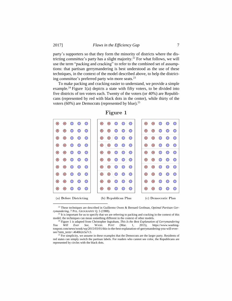
To make packing and cracking easier to understand, we provide a simple
example.24 Figure 1(a) depicts a state with fifty voters, to be divided into
five districts of ten voters each. Twenty of the voters (or 40%) are Republi-
cans (represented by red with black dots in the center), while thirty of the
voters (60%) are Democrats (represented by blue).25
22 These techniques are described in Guillermo Owen & Bernard Grofman, Optimal Partisan Ger-rymandering, 7 POL. GEOGRAPHY Q. 5 (1988).
23 It is important for us to specify that we are referring to packing and cracking in the context of this
model; the techniques can mean something different in the context of other models. 24 Figure 1 is adapted from Christopher Ingraham, This Is the Best Explanation of Gerrymandering
You Will Ever See, WASH. POST (Mar. 1, 2015), https://www.washing-
tonpost.com/news/wonk/wp/2015/03/01/this-is-the-best-explanation-of-gerrymandering-you-will-ever-see/?utm_term=.464bb2e3a7c3.
25 For simplicity, we assume in these examples that the Democrats are the larger party. Residents of
red states can simply switch the partisan labels. For readers who cannot see color, the Republicans are represented by circles with the black dots.
8 Journal of Law & Politics [Vol. XXXIII:1
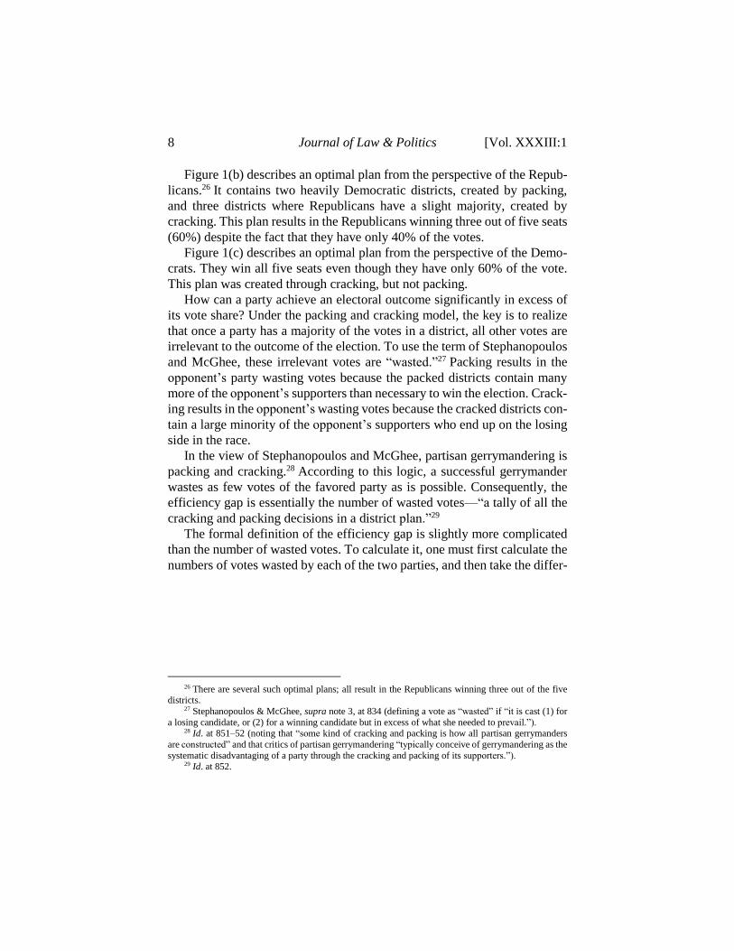
Figure 1(b) describes an optimal plan from the perspective of the Repub-
licans.26 It contains two heavily Democratic districts, created by packing,
and three districts where Republicans have a slight majority, created by
cracking. This plan results in the Republicans winning three out of five seats
(60%) despite the fact that they have only 40% of the votes.
Figure 1(c) describes an optimal plan from the perspective of the Demo-
crats. They win all five seats even though they have only 60% of the vote.
This plan was created through cracking, but not packing.
How can a party achieve an electoral outcome significantly in excess of
its vote share? Under the packing and cracking model, the key is to realize
that once a party has a majority of the votes in a district, all other votes are
irrelevant to the outcome of the election. To use the term of Stephanopoulos
and McGhee, these irrelevant votes are “wasted.”27 Packing results in the
opponent’s party wasting votes because the packed districts contain many
more of the opponent’s supporters than necessary to win the election. Crack-
ing results in the opponent’s wasting votes because the cracked districts con-
tain a large minority of the opponent’s supporters who end up on the losing
side in the race.
In the view of Stephanopoulos and McGhee, partisan gerrymandering is
packing and cracking.28 According to this logic, a successful gerrymander
wastes as few votes of the favored party as is possible. Consequently, the
efficiency gap is essentially the number of wasted votes—“a tally of all the
cracking and packing decisions in a district plan.”29
The formal definition of the efficiency gap is slightly more complicated
than the number of wasted votes. To calculate it, one must first calculate the
numbers of votes wasted by each of the two parties, and then take the differ-
26 There are several such optimal plans; all result in the Republicans winning three out of the five
districts. 27 Stephanopoulos & McGhee, supra note 3, at 834 (defining a vote as “wasted” if “it is cast (1) for
a losing candidate, or (2) for a winning candidate but in excess of what she needed to prevail.”). 28 Id. at 851–52 (noting that “some kind of cracking and packing is how all partisan gerrymanders
are constructed” and that critics of partisan gerrymandering “typically conceive of gerrymandering as the
systematic disadvantaging of a party through the cracking and packing of its supporters.”). 29 Id. at 852.
2017] Flaws in the Efficiency Gap 9
ence between these two numbers. The efficiency gap is this difference di-
vided by the total number of votes. 30 For any specific election, the efficiency
gap results in the same ranking of plans as the number of wasted votes.31
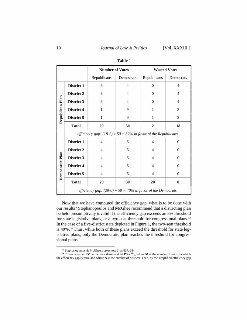
We demonstrate the efficiency gap in Table 1.
For the Republican plan (in Figure 1(b)), there are two types of districts;
three where the Republicans have six votes and the Democrats have four,
and two where the Republicans have one and the Democrats nine. In the
former districts, all six Republican votes are necessary to win the district,32
so the wasted votes are those of the four Democrats; in the latter districts,
only six of nine Democratic votes are necessary to win the district, so three
of the Democratic votes and the one Republican vote are counted as wasted.
This leads to a total of two wasted Republican votes and eighteen wasted
Democratic votes; because there are more wasted Democratic votes, we sub-
tract the former from the latter and we get a net of sixteen wasted Democratic
votes. Dividing by the total number of votes cast (fifty) gives us the effi-
ciency gap, which in this case is 32% (in favor of the Republicans).
For the Democratic plan (in Figure 1(c)), we repeat the exercise. Here,
for all five districts, the Republicans have four votes and the Democrats have
six. The result is that, in each district, it is the four Republican votes that are
wasted, as all six Democratic votes are necessary to win the district. This
leads to twenty wasted Republican votes. Because there are no wasted Dem-
ocratic votes, we simply divide this number by the total number of votes
cast, resulting in an efficiency gap of 40% (in favor of the Democrats).
30 This refers to the efficiency gap as defined in McGhee, supra note 3, and Stephanopoulos &
McGhee, supra note 3. However, there exist other versions; see Eric McGhee, Measuring Efficiency in
Redistricting, 16 ELECTION L.J. (forthcoming 2017), http://online.liebertpub.com/doi/pdf/10.1089/elj.2017.0453, which introduces a modified version of the
efficiency gap to account for a perceived problem of the original measure. (The problem is that the effi-ciency gap may fail to satisfy McGhee’s “efficiency principle” when districts do not have equal numbers
of voters. When districts do have equal numbers of voters, the original and modified measures coincide.) 31 The two definitions result in the same ranking of plans because the total number of wasted votes
is independent of the outcome of the vote. This implies that the number of wasted Republican votes can
be determined by knowing the number of wasted Democratic votes; it is simply the total number of
wasted votes minus the number of wasted Democratic votes. The extra complications in the efficiency gap formula are there only to make the efficiency gap scores easier to understand and to provide a sem-
blance of comparability across different elections and different states. In mathematical language, we
would say that the efficiency gap is “normalized.” 32 We ignore the possibility of a tie. In practice, ties are unpredictable and extremely rare.
10 Journal of Law & Politics [Vol. XXXIII:1
Table 1
Number of Votes Wasted Votes
Republicans Democrats Republicans Democrats
Pla
n
Rep
ub
lica
n
1 District 6 4 0 4
District 2 6 4 0 4
District 3 6 4 0 4
District 4 1 9 1 3
District 5 1 9 1 3
Total 20 30 2 18
efficiency gap: (18-2) ÷ 50 = 32% in favor of the Republicans
Pla
n
Dem
ocr
ati
c
1 District 4 6 4 0
District 2 4 6 4 0
District 3 4 6 4 0
District 4 4 6 4 0
District 5 4 6 4 0
Total 20 30 20 0
efficiency gap: (20-0) ÷ 50 = 40% in favor of the Democrats
Now that we have computed the efficiency gap, what is to be done with
our results? Stephanopoulos and McGhee recommend that a districting plan
be held presumptively invalid if the efficiency gap exceeds an 8% threshold
for state legislative plans, or a two-seat threshold for congressional plans.33
In the case of a five-district state depicted in Figure 1, the two-seat threshold
is 40%.34 Thus, while both of these plans exceed the threshold for state leg-
islative plans, only the Democratic plan reaches the threshold for congres-
sional plans.
33 Stephanopoulos & McGhee, supra note 3, at 837, 884. 34 To see why, let PV be the vote share, and let PS = M⁄N, where M is the number of seats for which
the efficiency gap is zero, and where N is the number of districts. Then, by the simplified efficiency gap
2017] Flaws in the Efficiency Gap 11
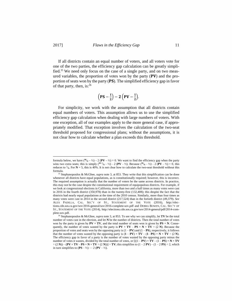
If all districts contain an equal number of voters, and all voters vote for
one of the two parties, the efficiency gap calculation can be greatly simpli-
fied.35 We need only focus on the case of a single party, and on two meas-
ured variables, the proportion of votes won by the party (𝐏𝐕) and the pro-
portion of seats won by the party (𝐏𝐒). The simplified efficiency gap in favor
of that party, then, is:36
(𝐏𝐒 −𝟏
𝟐) − 𝟐(𝐏𝐕 −
𝟏
𝟐).
For simplicity, we work with the assumption that all districts contain
equal numbers of voters. This assumption allows us to use the simplified
efficiency gap calculation when dealing with large numbers of voters. With
one exception, all of our examples apply to the more general case, if appro-
priately modified. That exception involves the calculation of the two-seat
threshold proposed for congressional plans; without the assumptions, it is
not clear how to calculate whether a plan exceeds this threshold.
formula below, we have (M⁄N – ½) – 2 (PV – ½) = 0. We want to find the efficiency gap when the party
wins two extra seats; this is simply (M+2⁄N – ½) – 2 (PV – ½). Because (M⁄N – ½) – 2 (PV – ½) = 0, this reduces to 2⁄N. For N = 5, this is 40%. It is not clear how to calculate the two-seat threshold without this
formula. 35 Stephanopoulos & McGhee, supra note 3, at 853. They write that this simplification can be done
whenever all districts have equal populations, as is constitutionally required; however, this is incorrect.
The required assumption is actually that the number of voters be the same across districts. In practice,
this may not be the case despite the constitutional requirement of equipopulous districts. For example, if we look at congressional elections in California, more than two and a half times as many votes were cast
in 2016 in the fourth district (350,978) than in the twenty-first (132,408); this despite the fact that the
districts had nearly equal populations at the time of the 2010 census. Similarly, more than four times as many votes were cast in 2014 in the second district (217,524) than in the fortieth district (49,379). See
ALEX PADILLA, CAL. SEC’Y OF ST., STATEMENT OF THE VOTE (2016), http://elec-
tions.cdn.sos.ca.gov/sov/2016-general/sov/2016-complete-sov.pdf and DEBRA BOWEN, CAL. SEC’Y OF
ST., STATEMENT OF THE VOTE (2014), http://elections.cdn.sos.ca.gov/sov/2014-general/pdf/2014-com-
plete-sov.pdf. 36 Stephanopoulos & McGhee, supra note 3, at 853. To see why we can simplify, let TV be the total
number of votes cast in the election, and let N be the number of districts. Then the total number of votes
won by the party is given by PV × TV, and the total number of seats won is given by PS × N. Conse-quently, the number of votes wasted by the party is PV × TV – PS × N × TV ÷ (2 N). Because the
proportion of votes and seats won by the opposing party is (1 – PV) and (1 – PS), respectively, it follows
that the number of votes wasted by the opposing party is (1 – PV) × TV – (1– PS) × N × TV ÷ (2 N). The efficiency gap in favor of a party is the number of votes wasted by the opposing party minus the
number of votes it wastes, divided by the total number of votes, or [((1 – PV) × TV – (1 – PS) × N × TV
÷ (2 N)) – (PV × TV – PS × N × TV ÷ (2 N))] ÷ TV; this simplifies to (1 – 2 PV) – (1 – 2 PS) ÷ 2, which in turn simplifies to (PS – ½) — 2 (PV – ½).
12 Journal of Law & Politics [Vol. XXXIII:1
Our criticism of the efficiency gap takes two parts. In Part III, we ask
whether the efficiency gap is a good way to test for partisan gerrymandering,
taking as given the assumptions of the packing and cracking model. In Part
IV, we ask whether these assumptions are themselves reasonable given the
goal of measuring partisan gerrymandering.
III. THE EFFICIENCY GAP AS A MEASURE OF PACKING AND CRACKING
In this Part, we assume, for the sake of argument, that the packing and
cracking story is a good explanation of partisan gerrymandering. We then
ask whether, given this assumption, we should use the efficiency gap to test
for partisan gerrymandering. Our conclusion is that we should not. The effi-
ciency gap relies on a flawed method of cost-benefit analysis; a correction
of this method leads us to a different measure. Furthermore, the proposed
thresholds for the application of the efficiency gap do not appear to have
been carefully thought out.
A. The Benefit of a Seat
The specific method used to measure wasted votes in the context of the
efficiency gap is controversial. The authors count all of a party’s votes as
wasted if the party loses in that district, and if the party wins in that district,
the authors count all of the party’s votes in excess of the 50% plus one
threshold necessary to win the district.37 Judge Griesbach’s dissent in Whit-
ford v. Gill, for example, criticized the wasted vote measure by using a sports
analogy, noting that the use of a similar method to calculate “wasted runs” in
baseball would be commonly understood to be absurd.38
The idea that parties want to minimize wasted votes seems natural. Waste
is a cost that comes without any benefit; most people want to minimize
waste. A wasted vote is a vote that perhaps could have been used in a differ-
ent district, to gain the party an extra seat.
However, few people work solely to minimize waste; instead, they seek
to balance costs with benefits. If votes are a cost, the benefits are seats. To
perform a cost-benefit analysis, we need to be able to compare votes and
seats. In this section, we make two claims: first, that the efficiency gap relies
on an implicit method of comparison, and second, that given the objective
of the efficiency gap, the wrong method of comparison is used.
37 This is 50% plus one-half if the number of voters is odd. 38 Whitford v. Gill, 218 F. Supp. 3d 837, 958 (W.D. Wis. 2016). The dissent’s criticism relies, in
essence, on the assumption that turnout is not fixed.
2017] Flaws in the Efficiency Gap 13
To understand our argument, it will help to focus on how the measure
applies to a single party, in a single district. Votes cast for the Republicans
can be wasted in two ways. First, all such votes are wasted if the Republicans
fail to win the district. Second, should the Republicans succeed, votes are
wasted if they are above the 50% plus one threshold required to win the
district.
Economists conduct cost-benefit analysis using the concepts of “mar-
ginal benefit” and “marginal cost.”39 In our context, the marginal benefit is
the gain the party receives from an additional vote in its favor; the marginal
cost is the cost of that extra vote. Typically, marginal benefits and costs are
measured in terms of dollars, but that is both difficult and unnecessary; it is
sufficient to measure these benefits and costs in terms of votes.
The marginal cost of a vote, measured in terms of votes, is always one
vote. This part is simple. What is the marginal benefit of a vote? Under the
efficiency gap, the marginal benefit of the first vote is zero: one vote is in-
sufficient to win the district. As there is a cost to this vote, but it results in
no benefit, it is deemed to be “wasted.” The same is true for the second,
third, and fourth votes, and for all votes up to (and including) the 50% thresh-
old.
For the first vote that passes the threshold, however, things are different.
That vote results in the party capturing the seat. The efficiency gap declares
it not wasted, and furthermore, it resets the measure of waste to zero, so that
all previous votes are now declared not to have been wasted. This implies
that the marginal benefit from capturing the seat is equal to the sum of the
marginal costs from all votes up to and including the deciding vote. Meas-
ured in terms of votes, then, the benefit of the seat is equal to the cost of 50%
plus one of the votes.
Every additional vote is counted by the efficiency gap as a wasted vote.
The marginal benefit from these votes is zero; the seat has already been won,
so they do no extra good. The marginal cost of these votes is still equal to
one vote. The efficiency gap can thus be understood as a measure of the
“relative inefficiency” of districting plans.40 It weights the costs against the
benefits for each party and then takes the difference in an attempt to deter-
mine, essentially, which party gets a better deal, and by how much. The ef-
ficiency gap is not the only possible relative inefficiency measure. There are
39 See, e.g., E.J. MISHAN, ELEMENTS OF COST-BENEFIT ANALYSIS (1972); BEN S. BERNANKE &
ROBERT H. FRANK, PRINCIPLES OF ECONOMICS 378 (3d ed. 2005). 40 For inefficiency in other contexts see Debreu, supra note 13, and Christopher P. Chambers & Alan
D. Miller, Inefficiency Measurement, 6 AM. ECON. J.: MICROECONOMICS 79 (2014). Importantly, once the population of voters is known, the total costs for either party are fixed and immutable.
14 Journal of Law & Politics [Vol. XXXIII:1
different ways to value the benefit from capturing the seat; each value im-
plies a different relative inefficiency measure.
Let us return to the thought experiment described in the introduction. Im-
agine a state that consists entirely of a single party; for example, all voters
are Republicans. This state would be ungerrymanderable; every conceivable
districting plan would result in 100% of the seats being captured by the Re-
publicans. A natural property of a desirable measure is that such a state
should be determined to be ungerrymandered. The efficiency gap, however,
would declare this state to be heavily gerrymandered in favor of the Demo-
crats: all wasted votes are Republican votes; the Democrats simply have no
votes to waste. This state would receive the worst possible score, almost
50%.
To put this in perspective, the efficiency gap treats this state as equivalent
to the case where the Democrats win every district by a single vote. To see
why, note that in this case, the Democrats still waste no votes; not because
they have no votes, but because they have exactly the number needed to win,
so none are wasted. All Republican votes are wasted, however, and all
wasted votes are Republican votes. So again, this state is judged to be heav-
ily gerrymandered in favor of the Democrats.
The hypothetical state where all voters are Republican is ungerrymander-
able; any reasonable measure of partisan gerrymandering should determine
it to be ungerrymandered. A measure of relative inefficiency will consider a
districting plan to be ungerrymandered if (and only if) the Democrats’ net
cost is equal to that of the Republicans.41 The Republicans, on the other
hand, pay the maximum cost (they receive all votes) and receive the maxi-
mum benefit (they win all seats). Their net cost must be equal to the net cost
of the Democrats, and this latter cost must be zero, because the Democrats
neither pay any cost (they receive no votes) nor receive any benefit (they
win no seats). An implication is that the benefit from winning all seats must
exactly equal the cost of receiving all of the votes. And this implies, in turn,
that the benefit of a single seat must be equal to all of the votes cast in that
district.42 Recall that the efficiency gap, instead, equated the benefit of a sin-
gle seat with approximately half of the votes cast in the district.
The idea that the benefit from winning a seat should be equal to the sum
of the votes cast in the district, and not simply half of the votes plus one,
41 The net cost is the cost minus the benefit. 42 Technically, this must be true on average; as mentioned earlier, we are keeping the assumption
that all districts have equal numbers of voters.
2017] Flaws in the Efficiency Gap 15
makes intuitive sense. The seat contains all of the political power in the dis-
trict. If a candidate wins an election with 60% of the vote, we think it is more
natural to say that this candidate has gained an advantage from the system
(having won all of the power with less than full support), than it is to say
that this candidate has suffered a loss.
The measure that results from our recalibration of the benefit of a seat
would also lead to a natural result in the hypothetical case where the Demo-
crats win every district by a single vote. In this case, the Democrats would
receive the maximum possible net benefit; that is, they would receive the
maximum possible benefit (all seats), and pay the minimum cost necessary
to get this benefit. The Republicans, by contrast, would pay the maximum
possible net cost; that is, they would receive no benefit (they win no seats),
but pay the maximum cost possible without winning any seats. Because the
Democrats’ net benefit is as far as is possible from the Republicans’ net cost,
the measure would in this case yield the same result as the efficiency gap,
assigning the worst possible score, and determining the state to be heavily
gerrymandered in favor of the Democrats.
The measure that results from our recalibration also leads to a metric that
is completely intuitive. Using the same notation as before for the proportion
of votes won by a party (𝐏𝐕) and the proportion of seats won by that party
(𝐏𝐒), the resulting measure (in favor of the party) is simply:43
𝐏𝐒 − 𝐏𝐕.
In other words, our recalibration of their metric leads to the difference
between the proportion of seats won and the proportion of votes won; as a
consequence, it associates the ideal situation with complete proportional-
ity.44
We emphasize here that we do not suggest that the different mathematical
equation we derive is appropriate for measuring partisan gerrymanders. In
43 To see why we can simplify, let TV be the total number of votes cast in the election, and let N be
the number of districts. Then the total number of votes won by the party is given by PV × TV, and the total number of seats won is given by PS × N. Consequently, the party’s net cost is PV × TV – PS × TV.
Because the proportion of votes and seats won by the opposing party is (1 – PV) and (1 – PS), respec-
tively, it follows that the net cost of the opposing party is (1 – PV) × TV – (1 – PS) × TV. The measure that results from our recalibration is the net cost of the opposing party minus the cost of the initial party,
divided by the total number of votes, or [((1 – PV) × TV – (1 – PS) × TV) – (PV × TV – PS × TV)] ÷
TV; this simplifies to 2 (PS – PV). Because the measure gives an identical ranking if transformed by a constant, we can simplify this to PS – PV.
44 If viewed as a measure of wasted votes, the measure that results from our recalibration would be
a counterexample to McGhee's claim, supra note 30, that the efficiency gap is the only measure of wasted votes that satisfies his efficiency principle.
16 Journal of Law & Politics [Vol. XXXIII:1
fact, we believe it is probably inappropriate. As we explain below, the im-
plicit benefit of a winning seat is only one of several problems with the effi-
ciency gap. Furthermore, the Supreme Court has in the past rejected the idea
that proportionality is required by the Constitution. Were proportionality the
ideal, it could easily be ensured without the Court’s interference by replacing
single-member legislative districts with a system of proportional elections.
The efficiency gap is not proportional in this sense; it does not imply that
the proportion of seats won should equal the proportion of votes won. Ra-
ther, it is quasi-proportional in the sense that it implies that the proportion of
seats should be a function of the proportion of votes: specifically, twice the
proportion of votes minus 50%. That is, it awards a “winner’s bonus” so that
an extra percent in the proportion of votes yields the party an extra two per-
cent in the proportion of seats awarded.45
Stephanopoulos and McGhee argue that quasi-proportionality is a posi-
tive attribute of the efficiency gap. However, it is hard to see why the effi-
ciency gap should be preferred on these grounds. McGhee points out that the
Supreme Court cases rejecting the idea that the Constitution requires pro-
portionality have not rejected their claim that the Constitution requires a
form of quasi-proportionality,46 but this issue has likely not been brought
before the Court.
Were the winner’s bonus implied by the efficiency gap the ideal, it could
also be implemented through a quasi-proportional voting system, in which
seats are awarded directly on the basis of the efficiency gap formula. Such a
system might be politically infeasible because it may be perceived as unfair,
but any such criticism would presumably apply to the efficiency gap as well.
If we do not advocate proportionality, why do we make this argument?
Our claim is more subtle. By taking the mathematical principles of measur-
ing “wasted votes,” and calibrating this idea using a scenario in which there
cannot be gerrymandering, we are led to an almost unmistakable conclusion,
and one that differs significantly from the efficiency gap.47 This merely sug-
gests that the implications of the efficiency gap have not been carefully con-
sidered.
45 Stephanolpoulos & McGhee, supra note 3, at 854. 46 Brief of Eric McGhee as Amicus Curiae in Support of Neither Party, Gill v. Whitford (U.S. will
argue Oct. 3, 2017) (No. 16-1161). 47 In this sense, our argument differs significantly from other researchers who have studied the effi-
ciency gap. See Cover, supra note 12, (referring to seats-votes proportionality as an important democratic
norm), and Bernstein & Duchin, supra note 12, (criticizing the efficiency gap as penalizing proportion-
ality). We do not assume that proportionality is a desirable feature of electoral outcomes or that a measure of partisan bias should be faulted for deviating from the proportionality norm. Our argument is that that
2017] Flaws in the Efficiency Gap 17
B. Scale Invariance and the Two-Seat Threshold
An efficiency gap of zero is essentially impossible due to randomness in
the electoral process.48 So that courts can apply the measure, its creators pro-
vide a test: redistricting legislation that results in an efficiency gap above a
certain threshold should be presumptively illegal, subject to a second-stage
judicial inquiry that they describe. They propose a specific threshold of two
seats for congressional plans and 8% for state legislative plans,49 and they
claim that it would be “hard to deny” the reasonableness of this proposal
even if “[s]cholars and judges may quibble” about the precise threshold.50
We disagree. As we explain, the two-seat threshold is clearly an unreasona-
ble measure of “how much partisan dominance is too much.”51
The problem with the two-seat threshold is that it imposes a stronger con-
straint in large states than in small states on the number of seats that a party
can be awarded. In fact, for the smallest states (those with no more than four
representatives), the efficiency gap with the two-seat threshold imposes no
constraint whatsoever on districting.52 Every possible plan is acceptable.53
The 8% threshold that Stephanopoulos and McGhee propose for state
legislative plans does not suffer from this scale-related problem. However,
it and all other fixed thresholds suffers from a different problem. There is a
possibility that it will reject every possible districting plan as being presump-
tively illegal.
logic of the efficiency gap itself compels proportionality; consequently, it is hard to justify using the efficiency gap when a proportionality standard could be used in its place.
48 Stephanopoulos & McGhee, supra note 3, at 887 (explaining that “almost every current plan”
would not have an efficiency gap of zero and that “plans’ efficiency gaps vary markedly from election to election”).
49 Id. at 884 (suggesting that “the bar be set at two seats for congressional plans and 8 percent for
state house plans”). The two-seat threshold is exactly 8% for states with twenty-five congressional dis-tricts, such as Florida following the 2000 Census.
50 Id. at 897–98. 51 Id. at 898, quoting League of United Latin Am. Citizens v. Perry, 548 U.S. 399, 420 (2006). 52 To prove this statement, note that a districting plan exceeds the threshold if
(PS – ½) – 2 (PV – ½) ≥ T. This expression is true if and only if PV ≤ ½ PS + ¼ – ½ T. Let PS = M⁄N,
where M is the number of seats won and N is the number of districts. Next, to win M districts requires that PV > M⁄2N. Thus, the districting plan exceeds the threshold if M⁄2N < PV ≤ M⁄2N + ¼ – ½ T, which is
possible if and only if T < ½. The two-seat threshold implies that T = 2⁄N ≥ ½ for N ≤ 4.∎ 53 The prior literature has noted that the efficiency gap does not work well in states with too few
districts. Cover, supra note 12, notes that the a two-seat threshold cannot be used to invalidate districting plans in two-district states; Cho, supra note 12, argues that the efficiency gap can only take on few dis-
crete values in states with few districts, a problem Bernstein & Duchin, supra note 12, refer to as
“nongranularity.” Our argument goes further and points out that this leads to a bias favoring a finding of partisan gerrymandering in large states as opposed to in small states.
18 Journal of Law & Politics [Vol. XXXIII:1
The efficiency gap with a two-seat threshold is a test that declares a dis-
tricting plan to be valid if a party has enough votes to justify the number of
seats it has won. How many votes does a party need for a plan to pass?
We begin with a simple example of a five-district state. Suppose that the
Republicans win 60% (or three) of the five districts. The Republicans cannot
win 60% of the seats unless they have more than 30% of the statewide vote,
as they need a majority in every district they win.54 The efficiency gap for-
mula tells us that they are below the threshold (and the plan passes the test)
if they receive more than 35% of the vote.55
The difference between these numbers, in this case 5%, is what we call
the “spare vote margin.” It is the percentage of the vote share above the the-
oretical minimum (half the proportion of seats won) that a party needs for
the plan to pass the test.
We have just established that, for the case of a five-district state and a
party that wins three seats, the spare vote margin is 5%. What about the case
of a five-district state and a party that wins all five seats? We know that the
party cannot win 100% of the seats with fewer than 50% of the votes. The
efficiency gap formula, meanwhile, tells us that the plan passes the test if the
party’s vote share exceeds 55%.56 The difference between these numbers—
the spare vote margin—is again 5%.
The fact that the spare vote margin was the same in these two cases is not
a coincidence. In fact, as we prove, the spare vote margin is determined en-
tirely by the number of districts in the state, and it is independent of the
number of districts won by the party. For a state with N districts, the spare
vote margin is expressed in terms of a percentage as:57
𝟐𝟓 −𝟏𝟎𝟎
𝐍.
54 They must win more than 50% of the votes in 60% of the districts; therefore, they must win more
than 50% × 60% = 30% of the votes in the state. 55The districting plan exceeds the threshold if (PS – ½) – 2 (PV – ½) ≥ T. In the example, PS = 60%
= ⅗, and the threshold T = ⅖. Substituting these values, we get (⅗ – ½) – 2 (PV – ½) ≥ ⅖, which is true
if and only if PV ≤ 0.35 = 35%. 56 The districting plan exceeds the threshold if (PS – ½) – 2 (PV – ½) ≥ T. In the example, PS =
100% =1, and the threshold T = ⅖. Substituting these values, we get (1 – ½) – 2 (PV – ½) ≥ ⅖, which is
true if and only if PV ≤ 0.55 = 55%. 57 For a threshold T and a vote share PS, the spare vote margin is given by PV* – ½ PS, where PV*
satisfies (PS – ½) – 2 (PV* – ½) = T. This latter expression reduces to PV* = ½ PS + ¼ – ½ T, which
implies that the spare vote margin is ¼ – ½ T. If we have N districts in the state, a two-seat threshold can
be expressed as 2⁄N; by making the substitution T = 2⁄N we get the expression ¼ – 1⁄N. Expressed in per-centage terms, this is 25 – 100⁄N.
2017] Flaws in the Efficiency Gap 19
The spare vote margin gives us a relatively simple way to think about the
consequences of changing the threshold. The larger the spare vote margin,
the stronger the constraint imposed by the test. Because the spare vote mar-
gin is larger in larger states, this implies that the efficiency gap with a two-
vote threshold constrains outcomes in large states more than it does in small
ones. To see why, consider the case in which a party wins 80% of the seats
with 50% of the vote. The plan will be approved as long as the party wins
more than the spare vote margin plus 40% of the votes.58 In a five-district
state, 80% is four districts, and the spare vote margin is 5%; the plan is ap-
proved, as 50% is greater than 45%. In a ten-district state, 80% is eight dis-
tricts, and the spare vote margin is 15%; thus the plan would fail, as 50% is
less than 55%.
The efficiency gap provides no constraint at all unless the spare vote mar-
gin is strictly positive. This is because a party cannot win a district through
a tie; it needs some spare votes to get a majority in the districts it wins. If the
spare vote margin is zero (or negative), it is impossible for a party to win the
seats yet have “too few” votes so as to fail the test. One can see from the
formula that, with a two-seat threshold, the spare vote margin is negative if
there are two or three districts in the state, and it is zero if there are four. It
follows that this test is vacuous for small states: those with no more than
four districts.
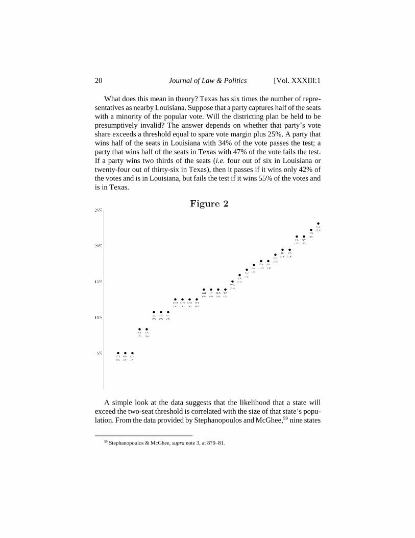
So the efficiency gap, with the two-seat threshold, treats large states dif-
ferently from small states. In other words, it is “scale dependent.” How
strong is this dependency? Under the Congressional apportionment follow-
ing the 2010 Census, twenty-nine states received five or more representa-
tives. Figure 2 depicts the spare vote margins for these states. The smallest
states (Connecticut, Oklahoma, and Oregon), with five representatives each,
all have a spare vote margin of 5%, as we explained above. The next smallest
states (Kentucky and Louisiana) have six representatives each, leading to a
spare vote margin of 8⅓%. The largest states, California (with fifty-three
representatives), Texas (thirty-six representatives), and New York and Flor-
ida (twenty-seven representatives each) have spare vote margins of over
23%, 22%, and 21%, respectively. The spare vote margin increases as the
number of districts grows, but does so at a decreasing rate. Louisiana has
20% more representatives than Oklahoma, but its spare vote margin is 66⅔%
larger; California has over 96% more representatives than New York, but its
spare vote margin is larger by only 8½%.
58 As before, it is impossible for the party to win 80% of the seats unless it wins more than 40% of
the votes. It must win 50% of the votes in 80% of the districts; 50% × 80% = 40%.
20 Journal of Law & Politics [Vol. XXXIII:1
What does this mean in theory? Texas has six times the number of repre-
sentatives as nearby Louisiana. Suppose that a party captures half of the seats
with a minority of the popular vote. Will the districting plan be held to be
presumptively invalid? The answer depends on whether that party’s vote
share exceeds a threshold equal to spare vote margin plus 25%. A party that
wins half of the seats in Louisiana with 34% of the vote passes the test; a
party that wins half of the seats in Texas with 47% of the vote fails the test.
If a party wins two thirds of the seats (i.e. four out of six in Louisiana or
twenty-four out of thirty-six in Texas), then it passes if it wins only 42% of
the votes and is in Louisiana, but fails the test if it wins 55% of the votes and
is in Texas.
A simple look at the data suggests that the likelihood that a state will
exceed the two-seat threshold is correlated with the size of that state’s popu-
lation. From the data provided by Stephanopoulos and McGhee,59 nine states
59 Stephanopoulos & McGhee, supra note 3, at 879–81.
2017] Flaws in the Efficiency Gap 21
had plans that passed the two-seat threshold in the decade following the 2000
Census. These nine states included the eight most populous states plus Mas-
sachusetts. For the decade following the 1990 Census, there were six such
states: five of the six largest states plus Washington, which curiously had a
districting plan that exceeded the two-seat threshold in favor of the Repub-
licans in one election and in favor of the Democrats in another. For the dec-
ade following the 1980 Census, there were again six such states: five of the
seven largest in addition to Massachusetts. The pattern is less apparent in the
decade that followed the 1970 Census: six of the ten states that passed the
threshold were at the time among the nine most populous.
By contrast, for state legislatures, Stephanopoulos and McGhee suggest
a threshold of 8%, independent of the size of the state or the number of leg-
islative districts. An 8% threshold is equivalent to a two-seat threshold in the
case where the state has exactly twenty-five districts. It is harder to see an
obvious bias related to the size of the state; for the decade following the 2000
Census, for example, the 8% threshold was exceeded by three of the five
most populous states (California, Florida, and New York, but not Pennsyl-
vania or Texas), and by three of the five least populous states for which data
is provided (Delaware, Vermont, and Wyoming, but not Alaska or Mon-
tana).60
We do not know whether a measure of gerrymandering should be entirely
independent of the size of the state or the number of legislative districts. For
example, if we were to agree that an imperfect measure was better than none,
and that this measure is more sensitive to gerrymandering in small states
than in large states, then it would make sense to adjust the threshold in larger
states to account for this sensitivity. But it is hard to see how one can justify
the extreme form of scale dependence that arises from the use of the two-
seat threshold. The bias created is so strong that it would render congres-
sional redistricting legislation in states such as Utah and Nevada immune
from constitutional scrutiny.
We do not advocate an alternative to the two-seat threshold proposed by
Stephanopoulos and McGhee. In part, this is because we do not believe that
the efficiency gap produces a meaningful ranking of districts. But in part, to
the extent that the efficiency gap may have some value, we do not believe
that it can be combined with a threshold to create a meaningful test.
Any test of gerrymandering should ideally have two properties. First, it
should sometimes reject districting plans; second, it should not reject all pos-
sible plans that could have been chosen. The first property requires that there
60 Id. at 882–84.
22 Journal of Law & Politics [Vol. XXXIII:1
should be some combinations of electoral outcomes and districting plans that
the test would reject as gerrymandered. We do not expect that a test be able
to reject district plans regardless of the electoral outcome, but we think it is
reasonable to expect that it sometimes be useful. The second property re-
quires that there be no election for which every plan would be deemed to be
presumptively illegal. The test of gerrymandering should not function as a
“Catch-22.”61
If the efficiency gap combined with a threshold is to satisfy the first prop-
erty, the threshold must be strictly below 50%. This is because, by definition,
the majority of votes in an election are not wasted, and therefore the effi-
ciency gap must be strictly below 50%. A threshold above the maximum
efficiency gap score would fail the first property because it could never re-
ject a districting plan.
If the threshold is below 50%, however, we are led to a different problem.
Recall the thought experiment where all voters vote Republican. All district
plans in this state receive the same score, and that score is the worst possible,
at nearly 50%. Every threshold below 50% will reject these plans, regardless
of the outcome of the election.
An analogous problem arises in states that are not completely Republi-
can. Consider, for example, a state where 80% of the votes for the state leg-
islature are cast for Republicans. Such a state will be deemed to have an
efficiency gap of at least 10% in favor of the Democrats. In this case, the 8%
threshold advocated by Stephanopoulos and McGhee would lead to the re-
jection of all possible districting plans.62
We recognize that one might respond by saying that the efficiency gap is
only intended to be used when the vote share is between 25% and 75%, and
for states where there are at least five districts, although these claims do not
appear in the Stephanopoulos and McGhee paper. There are several reasons
why we would disagree with this defense of the measure. First, it ignores the
nature of the thought experiment, which allows us to test our intuition in
settings where the right answer is clear. We have no reason to believe that
the failure of the efficiency gap in the thought experiment is not indicative
of a broader problem that affects the measurement of partisan gerrymander-
ing in large states where the vote share is between 25% and 75%.
61 JOSEPH HELLER, CATCH-22 (1961) (introducing the concept of the Catch-22).
2017] Flaws in the Efficiency Gap 23
Second, gerrymandering can still exist in states where one party has a
large majority, especially if the state is large, and in states with four or fewer
congressional districts. Democrats in Utah, for example, quite often believe
that state Republicans attempt to gerrymander both the state legislative and
federal congressional districts to minimize the Democrats’ voting power.63
Third, there is no clear justification for why 74% should be treated differ-
ently from 76%, or why a state with four districts is qualitatively different
from a state with five. Last, but not least, none of these distinctions are nec-
essary. As we have shown, the problems involving (a) states where one party
is dominant and (b) small states is an artifact of choosing the wrong measure
of benefit and the wrong threshold.
IV. THE PROBLEM OF PACKING AND CRACKING
In the previous part we asked whether the efficiency gap is a sensible
measure of packing and cracking, under the assumption that packing and
cracking is a good explanation of partisan gerrymandering. In this part, we
challenge that assumption. We argue that the packing and cracking story ig-
nores several considerations important to understand partisan gerrymander-
ing, and we show that, as a result of these considerations, a naïve application
of the efficiency gap can cause real harm.
A. Extremists
One of the most severe limitations of the efficiency gap is that it ignores
many of the intricacies inherent to the political process, and instead summa-
rizes a plan by two numbers: the number of seats awarded to each party, and
the number of votes attained by each party. While these numbers reveal the
number of Democrats and Republicans who get elected, they do not tell us
what kind of Democrats and Republicans these are; that is, whether they are
moderate, extreme, or somewhere in between. In other words, the efficiency
gap does not contemplate that political parties may be heterogeneous.
This is a problem because gerrymandering can affect not only which par-
ties are elected, but also the specific political opinions of the representatives
that comprise the legislature. The nature of these representatives is im-
portant; for example, the recent failure of the health bill was due to disagree-
ments between Republican factions, each of whom believed that the Afford-
able Care Act was flawed.
63 See, e.g., Paul Rolly, Rolly: Decades of Gerrymandering Bear Fruit: Utah's Legislature is Wacko,
SALT LAKE TRIB. (April 1, 2016), http://archive.sltrib.com/article.php?id=3727056&itype=CMSID.
24 Journal of Law & Politics [Vol. XXXIII:1
Unfortunately, the use of the efficiency gap by courts can lead to results
not anticipated by Stephanopoulos and McGhee. This is because the meas-
ure can favor plans that make it easier for political extremists to be elected,
and which would naturally increase the level of political polarization in leg-
islatures. More importantly, in spite of its proposed application in adjudicat-
ing Equal Protection cases, the use of the efficiency gap can actually harm
the minority party.
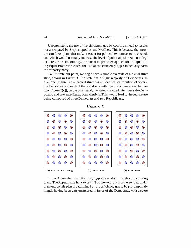
To illustrate our point, we begin with a simple example of a five-district
state, shown in Figure 3. The state has a slight majority of Democrats. In
plan one (Figure 3(b)), each district has an identical distribution of voters;
the Democrats win each of these districts with five of the nine votes. In plan
two (Figure 3(c)), on the other hand, the state is divided into three safe-Dem-
ocratic and two safe-Republican districts. This would lead to the legislature
being composed of three Democrats and two Republicans.
Table 2 contains the efficiency gap calculations for these districting
plans. The Republicans have over 44% of the vote, but receive no seats under
plan one, so this plan is determined by the efficiency gap to be presumptively
illegal, having been gerrymandered in favor of the Democrats, with a score
2017] Flaws in the Efficiency Gap 25
of over 44%.64 On the other hand, the Republicans receive two (or 40%) of
the seats under plan two; as a consequence, this plan receives a perfect score
of zero, and is presumptively legal. The efficiency gap thus provides a clear
answer to the question of which districting plan is preferred.65
Table 2
Number of Votes Wasted Votes
Democrats Republicans Democrats Republicans
On
e
Pla
n
1 District 5 4 0 4
District 2 5 4 0 4
District 3 5 4 0 4
District 4 5 4 0 4
District 5 5 4 0 4
Total 25 20 0 20
efficiency gap: (20-0) ÷ 45 = 44.44% in favor of the Democrats
Tw
o
Pla
n
1 District 9 0 4 0
District 2 8 1 3 1
District 3 8 1 3 1
District 4 0 9 0 4
District 5 0 9 0 4
Total 25 20 10 10
0% = 45 ÷ 20)-(20 gap: efficiency
64 In fact, this is the worst possible districting plan according to the efficiency gap. Forty-four percent
is above every threshold suggested by Stephanopoulos and McGhee. See Stephanopoulos & McGhee,
supra note 3, at 885–91. 65 Measures of partisan bias would generally give the opposite ranking, placing plan one ahead of
plan two.
26 Journal of Law & Politics [Vol. XXXIII:1
However, there are reasons to be suspicious of this result. First, while the
Republicans win two seats under plan two, the Democrats still have a ma-
jority and can pass legislation over the objections of the Republicans. It is
not clear why the seats make the Republicans better off. Second, the districts
in plan one appear more competitive. One might think that politicians
elected in politically lopsided districts may be more extreme than politicians
from politically competitive districts, and hence the legislature resulting
from plan two may be more polarized. The model used by Stephanopoulos
and McGhee to motivate the efficiency gap describes voters and politicians
only by their partisan affiliations, and does not provide a framework to dis-
tinguish between moderates and extremists.
To expand the analysis, we use the classical model of political competi-
tion introduced by the Scottish economist Duncan Black.66 The model envi-
sions political positions as being summarized by points on a line; each indi-
vidual has a policy on the line that they prefer the most.67 Voters care about
policy positions in a straightforward matter, referred to as “single-
peakedness” in the economics literature. As one moves further to the right
from their most preferred policy, they are made less well-off; they are simi-
larly harmed when the policy moves further to the left from their preferred
point.
The model conforms to common informal descriptions, so that the “left-
ists” are further to the left on the line, while “rightists” are further to the
right. Importantly, this model provides us with a language for describing
some voters as having more extreme positions than others. This framework
allows for much more generality than does a model that identifies people
only by their affiliation as Republicans or Democrats. At the same time, by
placing all of the voters on a line, it remains simple enough to provide us
with powerful insights.
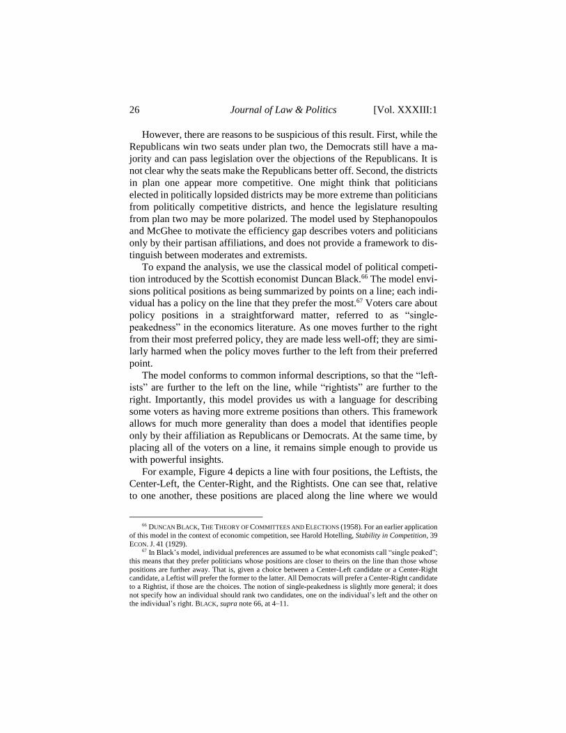
For example, Figure 4 depicts a line with four positions, the Leftists, the
Center-Left, the Center-Right, and the Rightists. One can see that, relative
to one another, these positions are placed along the line where we would
66 DUNCAN BLACK, THE THEORY OF COMMITTEES AND ELECTIONS (1958). For an earlier application
of this model in the context of economic competition, see Harold Hotelling, Stability in Competition, 39
ECON. J. 41 (1929). 67 In Black’s model, individual preferences are assumed to be what economists call “single peaked”;
this means that they prefer politicians whose positions are closer to theirs on the line than those whose
positions are further away. That is, given a choice between a Center-Left candidate or a Center-Right candidate, a Leftist will prefer the former to the latter. All Democrats will prefer a Center-Right candidate
to a Rightist, if those are the choices. The notion of single-peakedness is slightly more general; it does
not specify how an individual should rank two candidates, one on the individual’s left and the other on the individual’s right. BLACK, supra note 66, at 4–11.
2017] Flaws in the Efficiency Gap 27
naturally expect. The two more left-wing groups together comprise the Dem-
ocratic Party, while the two more right-wing ones form the Republicans.
Using this model, Black proved the most basic result in formal political
economy—the Median Voter Theorem—which states that under majority
rule, the selected alternative will be the one chosen by the median voter.
Recall that the median is a point for which half of the voters appear to the
left, and half are to the right. In political competition within districts, the seat
will be won by a politician whose position is located at the median of the
preferred points of the voters on the line. The policy chosen by the legisla-
ture, in turn, will be the policy advocated by the median politician.
For example, let us start with a simple example: a five-seat legislature
composed of three Democrats and two Republicans. Assume that two of the
Democrats are Leftists and that one is from the Center-Left. The median
legislator is the legislator from the Center-Left, because there are two legis-
lators to her left (the two Leftists) and two to her right (the Republicans).
The Median Voter Theorem predicts, then, that the chosen policy will be
that of the Center-Left. This explains why the Republicans might prefer to
have seats in the legislature. The Republican minority cannot get its own
policy adopted, but its presence results in a more conservative policy than
would be chosen by the Democrats alone.68
However, the intuition that more seats are better is not necessarily cor-
rect. Let us return to the example in Figure 3, but now, let us identify Dem-
ocrats as either Leftist or Center-Left, and Republicans as either Center-
Right or Rightist.69 Two districting plans are shown in Table 3. These plans
68 Recall that two out of three Democratic legislators are Leftists. 69 In our example, the Leftist group is larger than the other three. Note that the term Leftist in this
example is merely a label to denote the left-most 60% of the Democratic Party, while Center-Left denotes
the more moderate 40%. Other labels could be chosen. Our example does not depend on the idea that the leftmost 60% forms a coherent political block; in practice, we think one would find a wide range of views
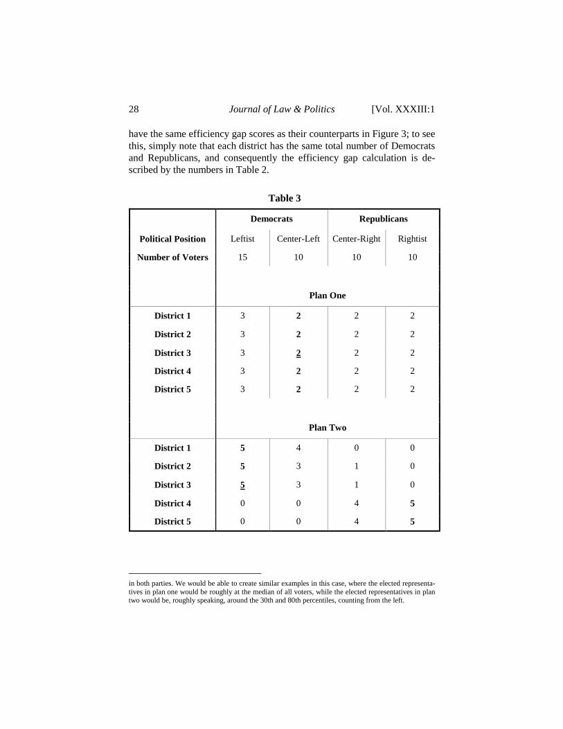
28 Journal of Law & Politics [Vol. XXXIII:1
have the same efficiency gap scores as their counterparts in Figure 3; to see
this, simply note that each district has the same total number of Democrats
and Republicans, and consequently the efficiency gap calculation is de-
scribed by the numbers in Table 2.
Table 3
Democrats Republicans
Political Position Leftist Center-Left Center-Right Rightist
Number of Voters 15 10 10 10
Plan One
1 District 3 2 2 2
District 2 3 2 2 2
District 3 3 2 2 2
District 4 3 2 2 2
District 5 3 2 2 2
Plan Two
1 District 5 4 0 0
District 2 5 3 1 0
District 3 5 3 1 0
District 4 0 0 4 5
District 5 0 0 4 5
in both parties. We would be able to create similar examples in this case, where the elected representa-
tives in plan one would be roughly at the median of all voters, while the elected representatives in plan two would be, roughly speaking, around the 30th and 80th percentiles, counting from the left.
2017] Flaws in the Efficiency Gap 29
As each district contains nine voters, the median voter in each district is
the fifth voter, counting from either the left or the right. This is because there
are four voters to the left of the median voter, and four voters to her right.
Voters in plan one are uniformly distributed; that is, each of the five dis-
tricts has an equal number of members of each group. Because there are five
Democratic voters in each district, the fifth voter must be among them; be-
cause there are only three Leftists in each district, that fifth voter cannot be
a Leftist. It follows then that the fifth, or median, voter must be a member of
the Center-Left. Because all five districts are identical, all five representa-
tives are Democrats from the Center-Left.
Plan two has been engineered to create safe districts for the two parties.
The three safe-Democratic districts (1–3) each contain five Leftists; this im-
plies that the fifth voter is also a Leftist. The safe-Republican districts each
contain five Rightists; this implies that the fifth voter in these districts must
be a Rightist. Thus this plan will result in a legislature with three Leftist
Democratic representatives and two Rightist Republican representatives.
The model predicts that the policies of the state legislature are determined
by the median of the elected representatives. Under plan one, all represent-
atives are members of the Center-Left, which implies that the plan would
lead to Center-Left policies. Under plan two, the majority of legislatures are
Leftists; this implies that the median, and consequently the chosen policy, is
that of the Leftists.
Which outcome is better depends, of course, on one’s political prefer-
ences. From the perspective of the Republicans, however, the consequences
are clear. All Republicans prefer the first plan, even though every seat is
captured by the Democrats.70 This is because Republicans are better off with
a Center-Left legislature than one controlled by the Leftists. The efficiency
gap, however, favors the second district plan, as demonstrated in Table 2.
This difference is important, because the efficiency gap has been touted as a
way to stop partisan gerrymandering. Yet, under the pretense that it is fairer
to Republicans, the efficiency gap would unambiguously choose the plan
that makes Republicans worse off.
B. Uncertainty
Figures 1 and 3 depicted a story of gerrymandering in which politicians
allocate voters into districts so as to maximize the number of seats their party
70 The model ignores the possibility that some voters might like to hold office, and only considers
the implemented policy.
30 Journal of Law & Politics [Vol. XXXIII:1
receives. However, in practice, that story is not entirely accurate. The main
problem is that politicians do not know where the voters are.
It is not that the politicians have no idea whatsoever about the voters’
locations; otherwise, there would be little point in gerrymandering. They
may have access to past election returns, the voters’ partisan affiliations,
census data including race and ethnicity, and other relevant information that
they can use. However, this doesn’t allow them to predict with certainty
whom the voters will choose or whether they will show up at the polls.
The efficiency gap does not rely on the information used by the gerry-
manderers, in part because it is not always clear what information they are
using. Instead, it measures the efficiency of a districting plan using the actual
votes from an election held under that plan. This is potentially problematic
for many reasons.
First, it is not entirely clear which is the group that may be denied Equal
Protection in an election. Is it the members of the Democratic party in the
state? Or is it the group of people who chose to vote for the Democratic
candidates in a particular election? If it is the former, then there is a problem
in that it is hard to tell who are the party members from election data; it is
known, after all, that voters do not always vote for their party’s candidates.
Furthermore, individuals vote differently across elections, and their voting
decisions are themselves affected by the districting plan. If it is the latter,
then there is a problem in that the relevant group changes from election to
election, so evidence from 2014 may not be relevant in determining whether
the districting plan denied Equal Protection to the group of Democratic vot-
ers in 2012. We are not the first to point out that this can be problematic; the
volatility of the efficiency gap was an issue considered by the district court
in Whitford v. Gill.
Second, the packing and cracking story upon which the efficiency gap
was founded may not hold if the partisan redistricting committee does not
know the outcomes of the elections in advance. Stephanopoulos and
McGhee justify the efficiency gap by explaining that partisan gerrymanders
are constructed through cracking and packing, and that, at “its core, [the ef-
ficiency gap] is nothing more than a tally of all the cracking and packing
decisions in a district plan.”71
However, it is by no means clear that packing and cracking is an optimal
strategy in the presence of uncertainty. A sizable literature has arisen in eco-
nomics and political science in which redistricting is treated as a classical
optimization problem, where a partisan in control of redistricting wants to
71 Stephanopoulos & McGhee, supra note 3, at 852.
2017] Flaws in the Efficiency Gap 31
maximize some numerical objective, usually the number of seats obtained
by a party.72 But these papers work in a framework of uncertainty, so that
when districts are drawn, it is not known exactly how votes will be distrib-
uted. Statistical models and assumptions will govern these hypotheses, and
the behavior of the partisan in the face of this uncertainty conforms to stand-
ard behavioral assumptions in the social sciences. The literature has not
reached a consensus, largely because uncertainty can be understood in sev-
eral different ways.73 There is also research showing that the strategy is not
optimal in the presence of geographic constraints.74
Third, judging a districting plan by the outcome of an election can itself
be problematic. As is generally acknowledged, elections contain a
significant random element. Using a single data point to determine whether
the districting plan was a consequence of partisan gerrymandering is similar
to trying to determine whether a coin is fair by flipping it once. For this
reason, the Supreme Court in Davis v. Bandemer explained that one cannot
establish partisan gerrymandering on the basis of a single election.75 Steph-
anopoulos and McGhee do suggest that “sensitivity analysis” be done as part
of the second stage of their test, but they do not explain how this should be
done, leading us to suspect that the analysis may be based on rather artificial
assumptions about voting behavior. It would make more sense to think about
the randomness of the election in devising the test in the first place.
While the issue of randomness has been discussed, we believe that the
problem is more serious than has been recognized.76 In particular, we want
to highlight two important problems. For the first, consider a state with two
congressional districts, where 67% of the voters are Democrats. There are
72 This literature was initiated by Owen & Grofman, supra note 22, who introduce the techniques of
packing and cracking. 73 See, e.g., John N. Friedman & Richard T. Holden, Optimal Gerrymandering: Sometimes Pack, but
Never Crack, 98 AM. ECON. REV. 113 (2008) (arguing that packing and cracking is not an optimal strat-egy under uncertainty); Faruk Gul & Wolfgang Pesendorfer, Strategic Redistricting, 100 AM. ECON.
REV. 1616 (2010) (showing conditions under which a generalized form of the the pack-and-crack strategy
is optimal); Hideo Konishi & Chen-Yu Pan, Partisan and Bipartisan Gerrymandering (B.C. Econ. Dep’t, Working Paper No. 922, 2016) (hypothesizing that partisan redistricters may care about both the number
of seats won and the political preferences of the politicians elected). 74 Clemens Puppe & Atilla Tasnádi, Optimal Redistricting Under Geographical Constraints: Why
“Pack and Crack” Does not Work, 105 ECON. LETTERS 93 (2009) (showing that the cracking and pack-
ing strategy may fail to be optimal when gerrymanderers face geographic constraints). 75 Davis v. Bandemer, 478 U.S. 109, 135 (1986) (“Relying on a single election to prove unconstitu-
tional discrimination is unsatisfactory.”). The decision also hinted that two elections would still not be
sufficient, by criticizing Justice Powell, who would, in their view, “allow a constitutional violation to be found where the only proven effect on a political party's electoral power was disproportionate results in
one election (possibly two elections).” Id. at 141. 76 A similar argument was raised by Cho, supra note 12, at 25 (noting that two different scenarios
that can lead to identical efficiency gap scores).
32 Journal of Law & Politics [Vol. XXXIII:1
two potential plans, shown in Table 4. Under the first plan, the Democrats
win the first district by 51% and the second district by 83%; under the second
plan, the Democrats win both districts by 67%.
Table 4
Number of Votes
Democrats Republicans
Plan One
1 District 51% 49%
District 2 83% 17%
Plan Two
1 District 67% 33%
District 2 67% 33%
From an ex ante perspective, these plans look very different. The first
plan contains one “competitive” district, in which the Democrats received
51% of the vote.77 One might view this as a sign that the legislature was
willing to take more risk. Furthermore, the existence of a competitive district
may have affected the electoral race and the resulting vote distribution. We
do not claim that the first plan is better than the second; but they are clearly
different. The efficiency gap, however, does not make a distinction between
these plans; because the overall Democratic vote share is the same under
both plans (67%) and because the Democrats win both seats, the two plans
have identical efficiency gap scores.
77 The district court in Davis v. Bandemer defined “competitive” districts as those in which “the
anticipated split in the party vote is within the range of 45% to 55%.” 478 U.S. at 130.
2017] Flaws in the Efficiency Gap 33
V. CONCLUSION
The efficiency gap is a flawed measure of partisan gerrymandering. Our
analysis suggests that it has not been carefully thought through in the rush
to have it enshrined in Constitutional law. The flaws are serious. The ranking
produced by the efficiency gap does not make sense in even the simplest of
settings. The application of the efficiency gap can increase polarization and
weaken political competition. It can harm the weaker party not in charge of
redistricting—despite its claim to help them.78
That we find flaws in the efficiency gap, however, does not mean that
there are no judicially manageable standards that courts can use to test for
partisan gerrymandering.79 It means, only, that we must work harder to find
them. Ideas should be carefully tested and subjected over time to serious
critical examination before they are used to affect policy.
The challenge of stopping gerrymandering is not figuring out how to con-
vince the Supreme Court. The challenge is in understanding gerrymandering
so that we can clearly recognize it, and so that courts can recognize it, too.
Until and unless meaningful standards are created to detect this behavior, or
meaningful algorithms are developed to take redistricting out of the hands
of partisans, it is difficult to blame the judges and the politicians for not
eliminating the problem once and for all.80
78 We note that Cover, supra note 12, and Bernstein & Duchin, supra note 12, argue for a limited
use of the efficiency gap by courts. They do not, however, provide much justification for their arguments. Cover argues that the efficiency gap does measure one significant democratic norm, without clearly ex-
plaining why the form of quasi-proportionality enshrined in the efficiency gap represents a significant
democratic norm. Bernstein and Duchin argue that the efficiency gap can be useful when the critiques they identified do not apply, and that the court should endorse the efficiency gap “only as a first draft of
a general standard that will be refined over time.” Bernstein & Duchin, supra note 12, at 5. We are not as comfortable with this proposal. If adopted by the Supreme Court, the efficiency gap in its current
formulation may significantly influence future redistricting to the voters' detriment. Furthermore, even if
its application were limited to cases where their critiques (as well as ours and those of other researchers) do not apply, the lack of careful though put into this measure hints that there may be additional prob-
lems lurking beneath the surface. This and other proposals to limit gerrymandering through formulas
require serious research before they should be applied by courts. 79 We offer no opinion on the other standards employed by the district court in Whitford v. Gill, 218
F. Supp. 3d 837 (W.D. Wis. 2016). 80 Of course, we can still blame the politicians who produce the heavily gerrymandered maps, just
not those who refuse to ban the practice because they do not know how.


![[Bob flaws] the_tao_of_healthy_eating_dietary](https://img.pdfslide.us/doc/110x75/55926e371a28ab9f5a8b46ab/bob-flaws-thetaoofhealthyeatingdietary.jpg)