F

JA

yirtz1tflflst

s

©

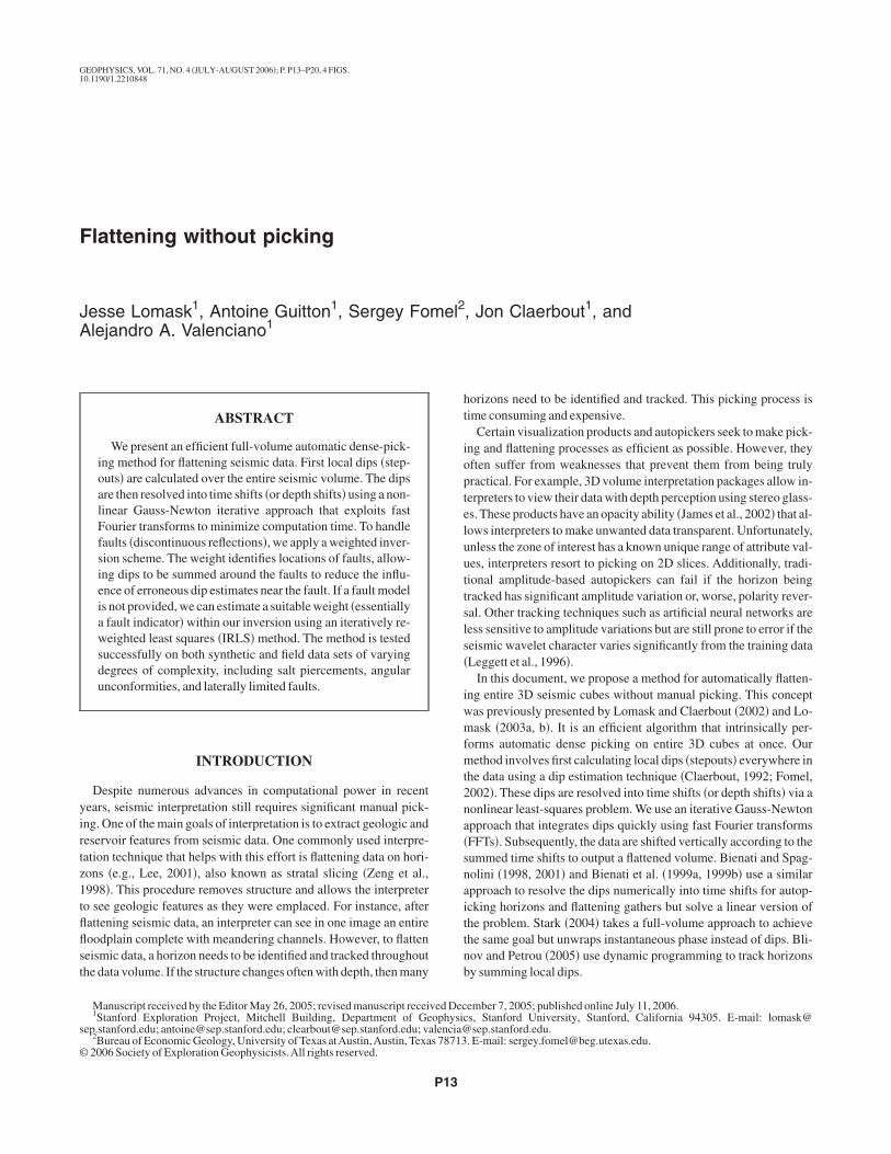
GEOPHYSICS, VOL. 71, NO. 4 �JULY-AUGUST 2006�; P. P13–P20, 4 FIGS.10.1190/1.2210848

lattening without picking

esse Lomask1, Antoine Guitton1, Sergey Fomel2, Jon Claerbout1, andlejandro A. Valenciano1

ht

iopteluuttsls�

iwmfmt2na�snaittnb

ved Decophysic

alencia@s 78713

ABSTRACT

We present an efficient full-volume automatic dense-pick-ing method for flattening seismic data. First local dips �step-outs� are calculated over the entire seismic volume. The dipsare then resolved into time shifts �or depth shifts� using a non-linear Gauss-Newton iterative approach that exploits fastFourier transforms to minimize computation time. To handlefaults �discontinuous reflections�, we apply a weighted inver-sion scheme. The weight identifies locations of faults, allow-ing dips to be summed around the faults to reduce the influ-ence of erroneous dip estimates near the fault. If a fault modelis not provided, we can estimate a suitable weight �essentiallya fault indicator� within our inversion using an iteratively re-weighted least squares �IRLS� method. The method is testedsuccessfully on both synthetic and field data sets of varyingdegrees of complexity, including salt piercements, angularunconformities, and laterally limited faults.

INTRODUCTION

Despite numerous advances in computational power in recentears, seismic interpretation still requires significant manual pick-ng. One of the main goals of interpretation is to extract geologic andeservoir features from seismic data. One commonly used interpre-ation technique that helps with this effort is flattening data on hori-ons �e.g., Lee, 2001�, also known as stratal slicing �Zeng et al.,998�. This procedure removes structure and allows the interpretero see geologic features as they were emplaced. For instance, afterattening seismic data, an interpreter can see in one image an entireoodplain complete with meandering channels. However, to flatteneismic data, a horizon needs to be identified and tracked throughouthe data volume. If the structure changes often with depth, then many

Manuscript received by the Editor May 26, 2005; revised manuscript recei1Stanford Exploration Project, Mitchell Building, Department of Ge

ep.stanford.edu; antoine@sep.stanford.edu; clearbout@sep.stanford.edu; v2Bureau of Economic Geology, University of Texas atAustin,Austin, Texa2006 Society of Exploration Geophysicists.All rights reserved.

P13

orizons need to be identified and tracked. This picking process isime consuming and expensive.

Certain visualization products and autopickers seek to make pick-ng and flattening processes as efficient as possible. However, theyften suffer from weaknesses that prevent them from being trulyractical. For example, 3D volume interpretation packages allow in-erpreters to view their data with depth perception using stereo glass-s. These products have an opacity ability �James et al., 2002� that al-ows interpreters to make unwanted data transparent. Unfortunately,nless the zone of interest has a known unique range of attribute val-es, interpreters resort to picking on 2D slices. Additionally, tradi-ional amplitude-based autopickers can fail if the horizon beingracked has significant amplitude variation or, worse, polarity rever-al. Other tracking techniques such as artificial neural networks areess sensitive to amplitude variations but are still prone to error if theeismic wavelet character varies significantly from the training dataLeggett et al., 1996�.

In this document, we propose a method for automatically flatten-ng entire 3D seismic cubes without manual picking. This conceptas previously presented by Lomask and Claerbout �2002� and Lo-ask �2003a, b�. It is an efficient algorithm that intrinsically per-

orms automatic dense picking on entire 3D cubes at once. Ourethod involves first calculating local dips �stepouts� everywhere in

he data using a dip estimation technique �Claerbout, 1992; Fomel,002�. These dips are resolved into time shifts �or depth shifts� via aonlinear least-squares problem. We use an iterative Gauss-Newtonpproach that integrates dips quickly using fast Fourier transformsFFTs�. Subsequently, the data are shifted vertically according to theummed time shifts to output a flattened volume. Bienati and Spag-olini �1998, 2001� and Bienati et al. �1999a, 1999b� use a similarpproach to resolve the dips numerically into time shifts for autop-cking horizons and flattening gathers but solve a linear version ofhe problem. Stark �2004� takes a full-volume approach to achievehe same goal but unwraps instantaneous phase instead of dips. Bli-ov and Petrou �2005� use dynamic programming to track horizonsy summing local dips.

ember 7, 2005; published online July 11, 2006.s, Stanford University, Stanford, California 94305. E-mail: lomask@sep.stanford.edu.

. E-mail: sergey.fomel@beg.utexas.edu.

aobbittscfwstfel

afifsscshf

cpdt�oeb1dt

mdptacIw

tossd

Bkci

w

firatdzncpTitnn

rfi

AavmsvmeiOcdseentteep

dar

P14 Lomask et al.

As with amplitude-based autopickers, amplitude variation alsoffects the quality of dip estimation and, in turn, impacts the qualityf our flattening method. However, the effect will be less significantecause our method can flatten the entire data cube at once — glo-ally — in a least-squares sense, minimizing the effect of poor dipnformation. Discontinuities in the data from faults tend to corrupthe local dip estimates at the faults. In this case, weights identifyinghe faults are applied within the iterative scheme, allowing recon-truction of horizons for certain fault geometries. Such weightsould be obtained from a previously determined fault model. If aault model is not provided, we automatically generate suitableeights using iteratively reweighted least squares �IRLS�. Once a

eismic volume is flattened, automatic horizon tracking becomes arivial matter of reversing the flattening process to unflatten flat sur-aces. The prestack applications for this method are numerous. Forxample, time shifts can be incorporated easily into an automatic ve-ocity-picking scheme �Guitton et al., 2004�.

In the following sections, we present the flattening methodologynd a series of real-world geologic challenges for this method. Therst is a 3D synthetic data set generated from a model with a dippingault and thinning beds. Then we present a structurally simple, 3Dalt piercement field data set from the Gulf of Mexico. We consider ittructurally simple because the geologic dips do not change signifi-antly with depth. Increasing complexity, we flatten a 3D field dataet from the North Sea that contains an angular unconformity andas significant folding. Last, we present a 3D faulted field data setrom the Gulf of Mexico.

FLATTENING THEORY

Ordinarily, to flatten a single surface, each sample is shifted verti-ally to match a chosen reference point. For instance, this referenceoint can be the intersection of the horizon and a well pick. In threeimensions, this reference point becomes a vertical line �referencerace�. To flatten 3D cubes, our objective is to find a mapping field�x,y,t� such that each time slice of this field contains the locations

f all data points along the horizon that happens to intersect the refer-nce trace at that time slice. We achieve this by summing dips. Theasic idea is similar to phase unwrapping �Ghiglia and Romero,994�; but instead of summing phase differences to get total phase,ips are summed to get total time shifts which are used then to flattenhe data.

The first step is to calculate local dips everywhere in the 3D seis-ic cube. Dips can be calculated efficiently using a local plane-wave

estructor filter as described by Claerbout �1992� or with an im-roved dip estimator described by Fomel �2002�. We primarily usehe latter. For each point in the data cube, two components of dip, bnd q, are estimated in the x- and y-directions, respectively. Thesean be represented everywhere on the mesh as b�x,y,t� and q�x,y,t�.f the data to be flattened are in depth, then dip is dimensionless, buthen the data are in time, dip has units of time over distance.Our goal is to find a time-shift �or depth-shift� field � �x,y,t� such

hat its gradient approximates the dip p�x,y,��. The dip is a functionf � because for any given horizon, the appropriate dips to beummed are the dips along the horizon itself. Using the matrix repre-entation of the gradient operator �� = � �

�x��y

�T� and the estimatedip �p = �b q�T�, our regression �developed inAppendix A� is

�� �x,y,t� = p�x,y,�� . �1�

ecause the estimated dip field p�x,y,�� is a function of the un-nown field � �x,y,t�, this problem is nonlinear and therefore diffi-ult to solve directly. We solve it using a Gauss-Newton approach byterating over the following equations:

r = ��k�x,y,t� − p�x,y,�k� , �2�

�� = ���T��−1�T�r , �3�

�k+1�x,y,t� = �k�x,y,t� + �� , �4�

here the subscript k denotes the iteration number.A more intuitive way to understand this method is to consider the

rst iteration. If no initial solution is provided, �0 will be zero and theesidual r will be the input dips p along each time slice. These dipsre then summed into time shifts using equation 3. At this point,hese time shifts can be used to flatten the data. However, because theips were summed along time slices and not along individual hori-ons, the data will not be perfectly flat. The degree that the data areot flat is related to the variability of the dip in time.At this point, weould reestimate new dips on the partially flattened data and then re-eat the process. Iterating in this way will eventually flatten the data.his is essentially how our method works, but instead of reestimat-

ng dips at each iteration, we correct the original dips at each itera-ion with equation 2. Not only is this more efficient than estimatingew dips at each iteration, but it is also more robust because disconti-uities introduced by flattening create inaccurate dips.

Convergence is generally reached when the change in normalizedesidual between consecutive iterations is smaller than a user-speci-ed tolerance �, i.e.,

�rk−1�− �rk��r0�

� �. �5�

value � = 0.001 often gives sufficiently flat results. An appealinglternative stopping criterion would be to consider only the absolutealue of the residual �rk� because it is essentially the sum of the re-aining dips. In this case, the stopping tolerance would be the user-

pecified minimum average dip value. Unfortunately, dip value isery sensitive to the amount of noise and, consequently, would notake a satisfactory stopping criterion. The stopping criterion in

quation 5 is less sensitive to the absolute value of the noise becauset considers only the change in residual from iteration to iteration.nce convergence is achieved, the resulting time-shift field � �x,y,t�

ontains all of the time shifts required to map the original unflattenedata to flattened data. This is implemented by applying the timehifts relative to a reference trace. In other words, each trace is shift-d to match the reference trace. For simplicity, we assume the refer-nce trace to be a vertical line; however, it could, in principle, beonvertical or even discontinuous. In general, we operate on oneime slice at a time. After iterating until convergence, we then selecthe next time slice and proceed down through the cube. In this way,ach time slice is solved independently. However, the number of it-rations can be significantly reduced by passing the solution of therevious time slice as an initial solution to the current time slice.

To improve efficiency greatly, we solve equation 3 in the Fourieromain using the FFT. We apply the divergence to the estimated dipsnd divide by the z-transform of the discretized Laplacian in the Fou-ier domain, i.e.,

wtTttraPse

ttsiie

Oadddr

itcn

sgmsteflt

W

pt

rpb

E

HFt

BFmts

I

fn1urWnatlffu

wMwspesd

lsoftdwfi

C

r

Flattening without picking P15

�� � FFT2D−1� FFT2D��Tr�

− Zx−1 − Zy

−1 + 4 − Zx − Zy� , �6�

here Zx = eiw�x and Zy = eiw�y. This fast Fourier approach is similaro the method of Ghiglia and Romero �1994� for unwrapping phase.his amounts to calling both a forward and inverse FFT at each itera-

ion. The ability to invert the 2D Laplacian in one step is the key tohe method’s computational efficiency. To avoid artifacts in the Fou-ier domain, we mirror the divergence of the residual �Tr before wepply the Fourier transform. Mirroring is described by Ghiglia andritt �1998� for application to 2D phase unwrapping. They also de-cribe a modification that uses cosine transforms instead of FFTs toliminate the need for mirroring.

The flattening process stretches or compresses the data in time, al-ering the spectrum. Even worse, the flattening process can disrupthe continuity of the data. To ensure a monotonic and continuous re-ult, one should first smooth the input dips in time �or depth�. In somenstances, it may be necessary to enforce smoothness while integrat-ng the dips. This can be accomplished by defining a 3D gradient op-rator with an adjustable smoothing parameter as

��� = ��

�x

��

�y

���

�t

� b

q

0 = p . �7�

ur new operator �� has a scalar parameter � used to control themount of vertical smoothing. In the case of flattening an image inepth, � is dimensionless; in the case of time, it has units of time overistance. This operator requires integrating the entire 3D volume ofips at once rather than slice by slice. The 2D FFTs in equation 6 areeplaced with 3D FFTs. Consequently, each iteration is slowed.

The magnitude of the smoothing parameter � depends on compet-ng requirements of the amount of noise and structural complexity. Ifhe structure is changing considerably with time, then it should behosen to be as small as possible. However, if there is significantoise resulting in erroneous dips, it should be larger.

There is a subtle difference between smoothing the input dips ormoothing the time-shift field. The time shift is essentially an inte-ration of the input dips, so small errors in the input dips can accu-ulate into large errors in the cumulative time-shift field. In the

ame way that traditional amplitude-based autopickers can get offhe intended horizon and jump to the wrong horizon by making onerror, merely smoothing the input dips can cause this algorithm toatten the wrong reflector. This is less likely to occur by smoothing

he time-shift field.

eighted solution for faults

Local dips estimated at fault discontinuities can be inaccurate. Torevent such inaccurate dips from adversely affecting the quality ofhe flattening, we can sum dips around the faults and ignore the spu-

ious dips across the faults to get a flattened result; a weighting is ap-lied to the residual to ignore fitting equations that are affected by thead dips estimated at the faults. The regression to be solved is now

W�� �x,y,t� = Wp�x,y,�� . �8�

quation 3 should then become

�� = ��TWTW��−1�TWTr . �9�

owever, because we cannot apply a nonstationary weight in theourier domain, we ignore the weights in equation 9 and iterate over

he same equations as before, except equation 2 is now replaced with

r = W���k�x,y,t� − p�x,y,�k�� . �10�

y ignoring the weights in equation 9, we are able to still use theourier method in equation 6. Naturally, this means that the Fourierethod is not approximating the inverse as well as before, causing

he algorithm to need more iterations to converge. This approach isimilar to that of Ghiglia and Romero �1994� for phase unwrapping.

RLS for fault weights

We also have an option of automatically creating the fault weightsrom the data cube itself within the inversion. It is known that the �1

orm is less sensitive to spikes in the residual �Claerbout and Muir,973�. Minimizing the �1 norm makes the assumption that the resid-als are exponentially distributed and have a long-tailed distributionelative to the Gaussian function assumed by the �2 norm inversion.

e can take advantage of this to honor dips away from faults and ig-ore inaccurate dips at faults. By iteratively recomputing a weightnd applying it in equation 10, we tend to ignore outlier dip valueshat occur at faults. By gradually ignoring more and more of the out-iers, the solution is no longer satisfying an �2 �least-squares� costunction but another more robust cost function. Our weight functionorces a Geman-McClure distribution �Geman and McClure, 1987�sing

W =1

�1 + r2/r̄2�2 , �11�

here r̄ is an adjustable damping parameter. We choose the Geman-cClure distribution because it is very robust and tends to createeights that are almost binary, much like a fault indicator. The re-

ulting fault indicator model is unique in that it represents the faulticks that best flatten the data. This IRLS approach adds consid-rably more iterations to the flattening process. Also, it dependstrongly on the quality of the data, precluding its use on very noisyata; with such data it tends to create false faults.

The damping parameter r̄ controls the sensitivity to outliers. If r̄ isarge, then the weight will be closer to one everywhere and, as a re-ult, almost all of the dips will be honored. If r̄ is small, more of theutlier dips will be ignored. If r̄ is too small, then dips that are not af-ected by faults and noise can be ignored, creating false faults. Prac-ice has shown that it is better to start out with a relatively largeamping parameter value of r̄ � 2 and then scale it by 0.8 when theeight is no longer changing. This generally means scaling it everyve IRLS iterations.

omputational cost

For a data cube with dimensions n = n1 � n2 � n3, each iterationequires n forward and reverse 2D FFTs. Therefore, the number of

1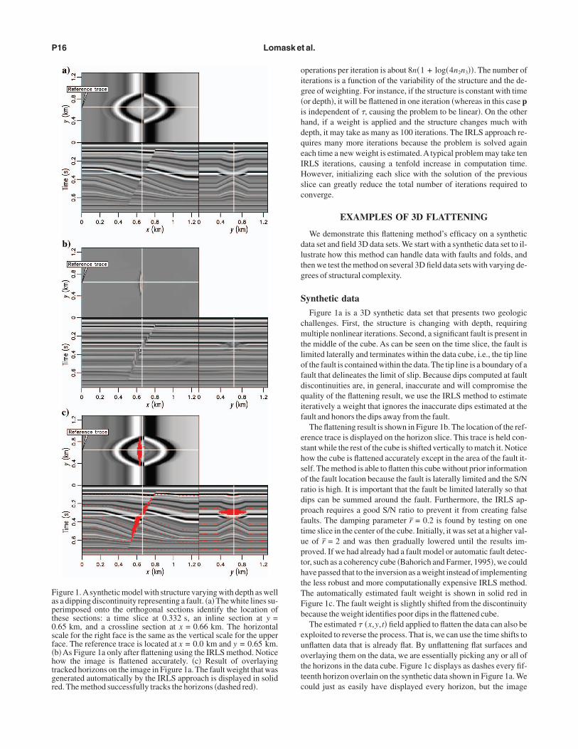

oig�ihdqeIHsc

dltg

S

cmtlofdqif

eshsordpftupthtTFb

euottc

Fapt0sf�htgred. The method successfully tracks the horizons �dashed red�.

P16 Lomask et al.

perations per iteration is about 8n�1 + log�4n2n3��. The number ofterations is a function of the variability of the structure and the de-ree of weighting. For instance, if the structure is constant with timeor depth�, it will be flattened in one iteration �whereas in this case ps independent of �, causing the problem to be linear�. On the otherand, if a weight is applied and the structure changes much withepth, it may take as many as 100 iterations. The IRLS approach re-uires many more iterations because the problem is solved againach time a new weight is estimated. A typical problem may take tenRLS iterations, causing a tenfold increase in computation time.owever, initializing each slice with the solution of the previous

lice can greatly reduce the total number of iterations required toonverge.

EXAMPLES OF 3D FLATTENING

We demonstrate this flattening method’s efficacy on a syntheticata set and field 3D data sets. We start with a synthetic data set to il-ustrate how this method can handle data with faults and folds, andhen we test the method on several 3D field data sets with varying de-rees of structural complexity.

ynthetic data

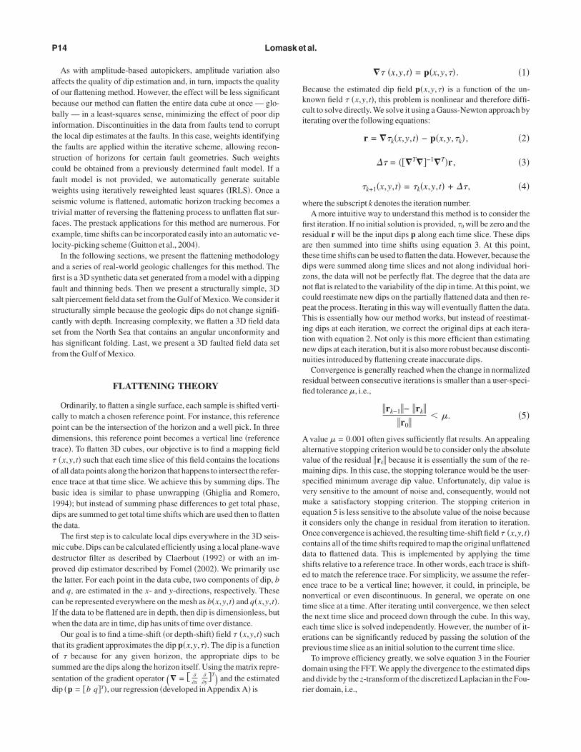
Figure 1a is a 3D synthetic data set that presents two geologichallenges. First, the structure is changing with depth, requiringultiple nonlinear iterations. Second, a significant fault is present in

he middle of the cube. As can be seen on the time slice, the fault isimited laterally and terminates within the data cube, i.e., the tip linef the fault is contained within the data. The tip line is a boundary of aault that delineates the limit of slip. Because dips computed at faultiscontinuities are, in general, inaccurate and will compromise theuality of the flattening result, we use the IRLS method to estimateteratively a weight that ignores the inaccurate dips estimated at theault and honors the dips away from the fault.

The flattening result is shown in Figure 1b. The location of the ref-rence trace is displayed on the horizon slice. This trace is held con-tant while the rest of the cube is shifted vertically to match it. Noticeow the cube is flattened accurately except in the area of the fault it-elf. The method is able to flatten this cube without prior informationf the fault location because the fault is laterally limited and the S/Natio is high. It is important that the fault be limited laterally so thatips can be summed around the fault. Furthermore, the IRLS ap-roach requires a good S/N ratio to prevent it from creating falseaults. The damping parameter r̄ = 0.2 is found by testing on oneime slice in the center of the cube. Initially, it was set at a higher val-e of r̄ = 2 and was then gradually lowered until the results im-roved. If we had already had a fault model or automatic fault detec-or, such as a coherency cube �Bahorich and Farmer, 1995�, we couldave passed that to the inversion as a weight instead of implementinghe less robust and more computationally expensive IRLS method.he automatically estimated fault weight is shown in solid red inigure 1c. The fault weight is slightly shifted from the discontinuityecause the weight identifies poor dips in the flattened cube.

The estimated � �x,y,t� field applied to flatten the data can also bexploited to reverse the process. That is, we can use the time shifts tonflatten data that is already flat. By unflattening flat surfaces andverlaying them on the data, we are essentially picking any or all ofhe horizons in the data cube. Figure 1c displays as dashes every fif-eenth horizon overlain on the synthetic data shown in Figure 1a. Weould just as easily have displayed every horizon, but the image

igure 1. Asynthetic model with structure varying with depth as wells a dipping discontinuity representing a fault. �a� The white lines su-erimposed onto the orthogonal sections identify the location ofhese sections: a time slice at 0.332 s, an inline section at y =.65 km, and a crossline section at x = 0.66 km. The horizontalcale for the right face is the same as the vertical scale for the upperace. The reference trace is located at x = 0.0 km and y = 0.65 km.b�As Figure 1a only after flattening using the IRLS method. Noticeow the image is flattened accurately. �c� Result of overlayingracked horizons on the image in Figure 1a. The fault weight that wasenerated automatically by the IRLS approach is displayed in solid

web

G

bbsst

flczucncs

FwsT

N

MtrwpeiHne

dTsawi

G

ffir̄ssaflhw

Fptcftbswctem

Flattening without picking P17

ould appear too cluttered. Notice that the horizons are well tracked,ven across a fault. Additionally, the slight shifts in fault weight cane removed by unflattening the fault weight itself.

ulf of Mexico salt piercement data

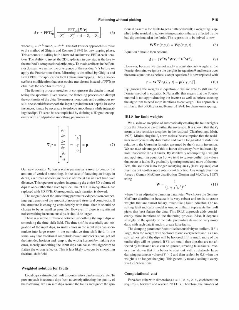
Figure 2a is a field 3D data cube from the Gulf of Mexico providedy Chevron. It consists of structurally simple horizons that haveeen warped up around a salt piercement. Several channels can beeen in the time slice at the top of Figure 2a, but they are largely ob-cured by the gradual amplitude overprint of a nearly flat horizonhat is cut by the time slice.

Figure 2b shows the flattened output of the data in Figure 2a. Weattened this data set using the method without weights. The seismicube has been converted from a stack of time slices to a stack of hori-on slices. Notice that the gradual amplitude overprint present in thenflattened data is no longer present in the flattened data. This is be-ause horizons are no longer cutting across the image. Several chan-els are now easily visible on the horizon slice. Also, the beds adja-ent to the salt dome have been partially reconstructed, causing thealt to occupy a smaller area in Figure 2b.

Figure 2c displays three horizons overlain on the original data inigure 2a. The horizons track the reflectors on the flanks of the saltell. Within the salt, the horizons gradually diverge from their re-

pective reflector events as the estimated dip becomes less accurate.he time slice at the top displays the swath of a tracked horizon.

orth Sea unconformity data

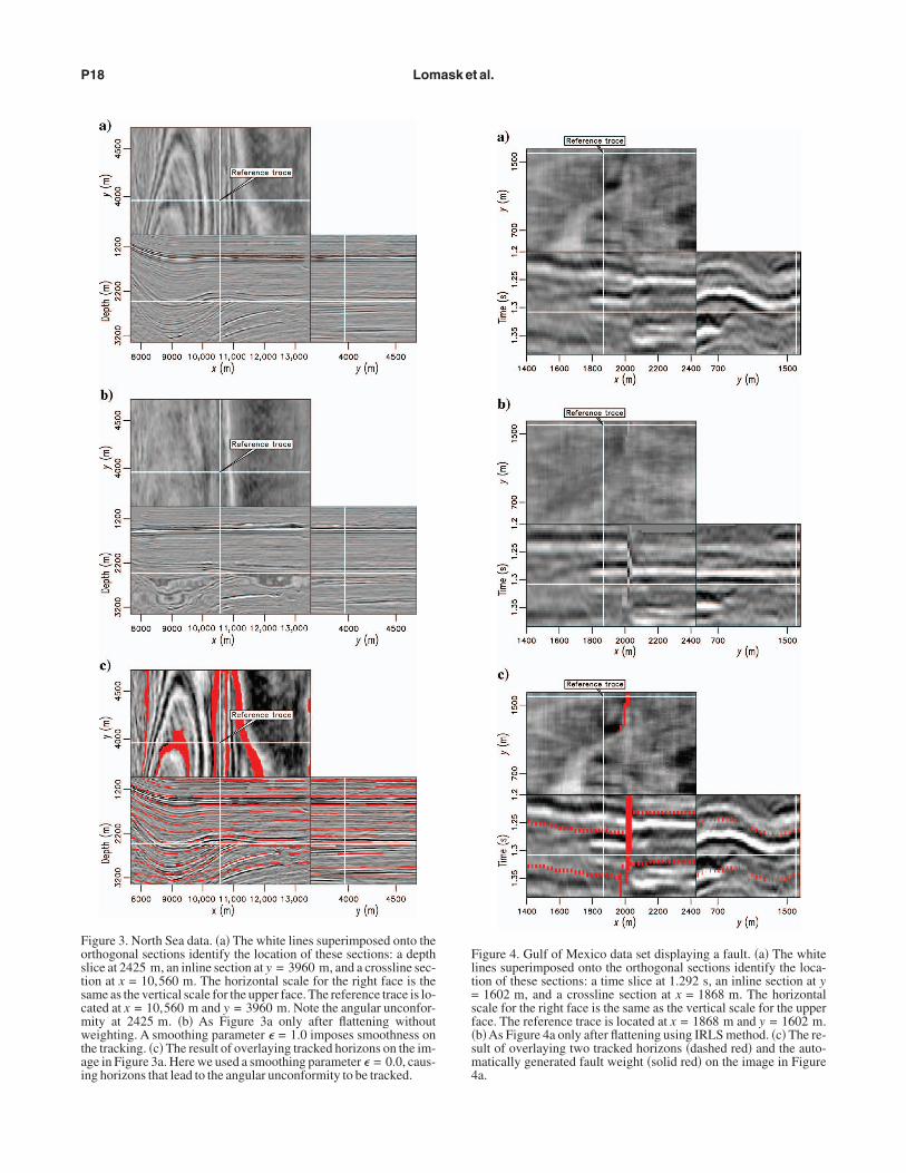
Figure 3a shows a 3D North Sea data set provided by Total.arked by considerable folding and a sharp angular unconformity,

his data set presents a real-world flattening challenge. The flatteningesult shown in Figure 3b was made using the method withouteights. To preserve the continuity of the data, we used a smoothingarameter of � = 1.0 in equation 7. We estimated � through trial andrror and aimed to make it as small as possible while preserving themage quality. As a result, the flattened data are not completely flat.ad we used � = 0.0, the data would be flatter but would lose conti-uity. Consequently, the trade-off between continuity and flatnessmerges in cases of pinch-outs and unconformities.

To achieve good agreement between the tracked horizons and theata, we found � = 0.0 to be preferable, i.e., no imposed continuity.he result is shown in Figure 3c. The time slice at the top shows thewaths of a few horizons. Overall, the tracked horizons track up tond along the unconformity, although some significant errors occurhere the data quality is poor and, as a result, the estimated dips are

naccurate.

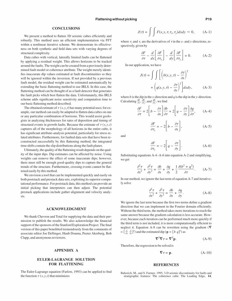
ulf of Mexico faulted data

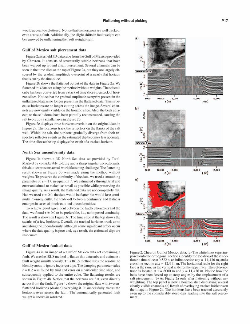
Figure 4a is an image of a Gulf of Mexico data set containing aault. We use the IRLS method to flatten this data cube and estimate aault weight simultaneously. This IRLS method uses the residual todentify areas to ignore incorrect dips. The damping parameter value= 0.2 was found by trial and error on a particular time slice, and

ubsequently applied to the entire cube. The flattening results arehown in Figure 4b. Notice that the horizons are flat, even directlycross from the fault. Figure 4c shows the original data with two un-attened horizons �dashed� overlying it. It successfully tracks theorizons even across the fault. The automatically generated faulteight is shown in solid red.

igure 2. Chevron Gulf of Mexico data. �a� The white lines superim-osed onto the orthogonal sections identify the location of these sec-ions: a time slice at 0.522 s, an inline section at y = 11,436 m, and arossline section at x = 12,911 m. The horizontal scale for the rightace is the same as the vertical scale for the upper face. The referencerace is located at x = 8000 m and y = 11,436 m. Notice how theeds have been forced up to steep angles by the emplacement of aalt piercement. �b� As Figure 2a only after flattening without anyeighting. The top panel is now a horizon slice displaying several

learly visible channels. �c� Result of overlaying tracked horizons onhe image in Figure 2a. The horizons have been tracked accuratelyven up to the considerably steep dips leading into the salt pierce-ent.

Fostscmwtai

Flt=sf�sm4

P18 Lomask et al.

igure 3. North Sea data. �a� The white lines superimposed onto therthogonal sections identify the location of these sections: a depthlice at 2425 m, an inline section at y = 3960 m, and a crossline sec-ion at x = 10,560 m. The horizontal scale for the right face is theame as the vertical scale for the upper face. The reference trace is lo-ated at x = 10,560 m and y = 3960 m. Note the angular unconfor-ity at 2425 m. �b� As Figure 3a only after flattening withouteighting. A smoothing parameter � = 1.0 imposes smoothness on

he tracking. �c� The result of overlaying tracked horizons on the im-ge in Figure 3a. Here we used a smoothing parameter � = 0.0, caus-ng horizons that lead to the angular unconformity to be tracked.

igure 4. Gulf of Mexico data set displaying a fault. �a� The whiteines superimposed onto the orthogonal sections identify the loca-ion of these sections: a time slice at 1.292 s, an inline section at y

1602 m, and a crossline section at x = 1868 m. The horizontalcale for the right face is the same as the vertical scale for the upperace. The reference trace is located at x = 1868 m and y = 1602 m.b�As Figure 4a only after flattening using IRLS method. �c� The re-ult of overlaying two tracked horizons �dashed red� and the auto-atically generated fault weight �solid red� on the image in Figure

a.

rwns

bamfiwfefltso

aogschlct

iwttt

btips

msvaC

Tt

ws

wC

a

Sw

Il

WdWsetn=

T

B

Flattening without picking P19

CONCLUSIONS

We present a method to flatten 3D seismic cubes efficiently andobustly. This method uses an efficient implementation via FFTithin a nonlinear iterative scheme. We demonstrate its effective-ess on both synthetic and field data sets with varying degrees oftructural complexity.

Data cubes with vertical, laterally limited faults can be flattenedy applying a residual weight. This allows horizons to be trackedround the faults. The weight can be created from a previously deter-ined fault model or coherence attribute. The weight merely identi-es inaccurate dip values estimated at fault discontinuities so theyill be ignored within the inversion. If not provided by a previous

ault model, the residual weight can be estimated automatically byxtending the basic flattening method to use IRLS. In this case, theattening method can be thought of as a fault detector that generates

he fault picks which best flatten the data. Unfortunately, this IRLScheme adds significant noise sensitivity and computation time tour basic flattening method described.

The obtained estimate of � �x,y,t� has many potential uses; for ex-mple, our method can easily be adapted to flatten data cubes on oner any particular combination of horizons. This would assist geolo-ists in analyzing thicknesses for rates of deposition and timing oftructural events in growth faults. Because the estimate of � �x,y,t�aptures all of the morphology of all horizons in the entire cube, itas significant attribute-analysis potential, particularly for stress re-ated attributes. Furthermore, for faulted data sets that have been re-onstructed successfully by this flattening method, the integratedime shifts contain the slip distributions along the fault planes.

Ultimately, the quality of the flattening result depends on the qual-ty of the input dips. Dip estimates can be affected by noise. Usingeights can remove the effect of some inaccurate dips; however,

here must still be enough good-quality dips to capture the generalrends of the structure. Furthermore, crossing events cannot be flat-ened easily by this method.

We envision a tool that can be implemented quickly and easily onoth poststack and prestack data sets, exploiting its superior compu-ational performance. For poststack data, this method can provide annitial picking that interpreters can then adjust. The potentialrestack applications include gather alignment and velocity analy-is.

ACKNOWLEDGMENT

We thank Chevron and Total for supplying the data and their per-ission to publish the results. We also acknowledge the financial

upport of the sponsors of the Stanford Exploration Project. The finalersion of this paper benefitted tremendously from the comments ofssociate editor Joe Dellinger, Huub Douma, Peeter Akerberg, Boblapp, and anonymous reviewers.

APPENDIX A

EULER-LAGRANGE SOLUTIONFOR FLATTENING

he Euler-Lagrange equation �Farlow, 1993� can be applied to findhe function � �x,y,t� that minimizes

J��� = � � F�x,y,�,�x,�y�dxdy � 0, �A-1�

here �x and �y are the derivatives of � in the x- and y-directions, re-pectively, given by

�F

��−

d

dx� �F

��x� −

d

dy� �F

��y� = 0. �A-2�

In our application, we have

J��� = � � ��b�x,y,�� −��

�x 2

+ �q�x,y,�� −��

�y 2�dxdy , �A-3�

here b is the dip in the x-direction and q is the dip in the y-direction.alculating �F

�� , �F��x

, and �F��y

, we find

�F

��= 2�b −

��

�x� �b

��+ 2�q −

��

�y� �q

��, �A-4�

�F

��x= − 2�b −

��

�x� , �A-5�

nd

�F

��y= − 2�q −

��

�y� . �A-6�

ubstituting equations A-4–A-6 into equation A-2 and simplifying,e get

�2�

�x2 +�2�

�y2 =�b

�x+

�q

�y+

1

2

��b2 + q2���

. �A-7�

n our method, we ignore the last term of equation A-7 and iterative-y solve

�2�

�x2 +�2�

�y2 =�b

�x+

�q

�y. �A-8�

e ignore the last term because the first two terms define a gradientirection that we can implement in the Fourier domain efficiently.ithout the third term, the method takes more iterations to reach the

ame answer because the gradient calculation is less accurate. How-ver, because each iteration can be performed much more quickly ifhe third term is not included, it is more computationally efficient toeglect it. Equation A-8 can be rewritten using the gradient ��

� ��x

��y �T� and the estimated dip �p = �b q�T� as

�T�� = �Tp . �A-9�

herefore, the regression to be solved is

�� = p . �A-10�

REFERENCES

ahorich, M., and S. Farmer, 1995, 3-D seismic discontinuity for faults andstratigraphic features: The coherence cube: The Leading Edge, 14,

B

—

B

—

B

C

C

F

F

G

G

G

G

J

L

L

L

L

—

S

Z

P20 Lomask et al.

1053–1058.ienati, N., and U. Spagnolini, 1998, Traveltime picking in 3D data volumes:60thAnnual Meeting, EAGE, ExtendedAbstracts, Session 01-12.—–, 2001, Multidimensional wavefront estimation from differential de-lays: IEEE Transactions on Geoscience and Remote Sensing, 39,655–664.

ienati, N., M. Nicoli, and U. Spagnolini, 1999a, Automatic horizon pickingalgorithms for multidimensional data: 61st Annual Meeting, EAGE, Ex-tendedAbstracts, Session 6030.—–, 1999b, Horizon picking for multidimensional data: An integrated ap-proach: 6th International Congress, Brazilian Geophysical Society, Pro-ceedings, SBGf359.

linov, A., and M. Petrou, 2005, Reconstruction of 3-D horizons from 3-Ddata sets: Institute of Electrical and Electronics Engineers, Geoscience andRemote Sensing, 43, 1421–1431.

laerbout, J. F., 1992, Earth soundings analysis: Processing versus inver-sion: Blackwell Scientific Publications.

laerbout, J. F., and F. Muir, 1973, Robust modeling with erratic data: Geo-physics, 38, 826–844.

arlow, S. J., 1993, Partial differential equations for scientists and engineers:Dover Publications.

omel, S., 2002, Applications of plane-wave destruction filters: Geophysics,67, 1946–1960.

eman, S., and D. McClure, 1987, Statistical methods for tomographic im-age reconstruction: Bulletin of the International Statistical Institute, L, no.II, 4–5.

higlia, D. C., and M. D. Pritt, 1998, Two-dimensional phase unwrapping:Theory, algorithms, and software: John Wiley & Sons, Inc.

higlia, D. C., and L. A. Romero, 1994, Robust two-dimensional weightedand unweighted phase unwrapping that uses fast transforms and iterativemethods: Optical Society ofAmerica, 11, no. 1, 107–117.

uitton, A., J. F. Claerbout, and J. M. Lomask, 2004, First order interval ve-locity estimates without picking: 74th Annual International Meeting,SEG, ExpandedAbstracts, 2339–2342.

ames, H., A. Peloso, and J. Wang, 2002, Volume interpretation of multi-at-tribute 3D surveys: First Break, 20, no. 3, 176–180.

ee, R., 2001, Pitfalls in seismic data flattening: The Leading Edge, 20, no.1, 160–164.

eggett, M., W. A. Sandham, and T. S. Durrani, 1996, 3D horizon trackingusing artificial neural networks: First Break, 14, 413–418.

omask, J., and J. Claerbout, 2002, Flattening without picking: Stanford Ex-ploration Project Report, 112, 141–149.

omask, J., 2003a, Flattening 3D seismic cubes without picking: 73rdAnnu-al International Meeting, SEG ExpandedAbstracts, 1402–1405.—–, 2003b, Flattening 3-D data cubes in complex geology: Stanford Ex-ploration Project Report, 113, 249–259.

tark, T. J., 2004, Relative geologic time �age� volume — Relating everyseismic sample to a geologically reasonable horizon: The Leading Edge,23, 928–932.

eng, H., M. M. Backus, K. T. Barrow, and N. Tyler, 1998, Stratal slicing,part I: Realistic 3D seismic model: Geophysics, 63, 502–513.