Working Paper/Document de travail 2011-21

Fixed-Term and Permanent Employment Contracts: Theory and Evidence

by Shutao Cao, Enchuan Shao and Pedro Silos

2

Bank of Canada Working Paper 2011-21

October 2011

Fixed-Term and Permanent Employment Contracts: Theory and Evidence

by

Shutao Cao,1 Enchuan Shao2 and Pedro Silos3

1Canadian Economic Analysis Department Bank of Canada

Ottawa, Ontario, Canada K1A 0G9 shutacao@bankofcanada.ca

2Currency Department

Bank of Canada Ottawa, Ontario Canada K1A 0G9

eshao@bankofcanada.ca

3Federal Reserve Bank of Atlanta Atlanta, Georgia 30309 pedro.silos@atl.frb.org

Bank of Canada working papers are theoretical or empirical works-in-progress on subjects in economics and finance. The views expressed in this paper are those of the authors.

No responsibility for them should be attributed to the Bank of Canada, the Federal Reserve Bank of Atlanta or the Federal Reserve System.

ISSN 1701-9397 © 2011 Bank of Canada

ii

Acknowledgements

We appreciate comments and suggestions from participants at the University of Iowa, the Bank of Canada, the Search and Matching Workshop in Konstanz (2010) (especially our discussant Georg Duernecker), Midwest Macroeconomics Meetings, Computing in Economics and Finance Meetings, the Canadian Economics Association Meetings, the Matched Employer-Employee Conference in Aarhus, and especially Shouyong Shi and David Andolfatto. Finally, we would like to thank Yves Decady at Statistics Canada for his assistance with the WES data.

iii

Abstract

This paper constructs a theory of the coexistence of fixed-term and permanent employment contracts in an environment with ex-ante identical workers and employers. Workers under fixed-term contracts can be dismissed at no cost while permanent employees enjoy labor protection. In a labor market characterized by search and matching frictions, firms find it optimal to discriminate by offering some workers a fixed-term contract while offering other workers a permanent contract. Match-specific quality between a worker and a firm determines the type of contract offered. We analytically characterize the firm’s hiring and firing rules. Using matched employer-employee data from Canada, we estimate the model’s parameters. Increasing the level of firing costs increases wage inequality and decreases the unemployment rate. The increase in inequality results from a larger fraction of temporary workers and not from an increase in the wage premium earned by permanent workers.

JEL classification: H29, J23, J38 Bank classification: Labour markets; Potential output; Productivity

Résumé

Les auteurs élaborent un cadre théorique pour expliquer la coexistence de contrats à durée déterminée et de contrats de travail permanents dans un milieu où travailleurs et employeurs sont a priori identiques. Les travailleurs temporaires sont licenciables sans frais, alors que les employés permanents jouissent d’une protection d’emploi. Sur un marché du travail caractérisé par des frictions dans la prospection et l’appariement, les entreprises jugent optimal d’opérer des distinctions en proposant à certains travailleurs un contrat à durée déterminée et à d’autres un contrat permanent. La qualité intrinsèque de l’appariement entre le travailleur et l’entreprise motive le choix du contrat offert. Les auteurs définissent par analyse les règles d’embauche et de congédiement des entreprises. Les paramètres du modèle sont estimés à l’aide de données canadiennes relatives au jumelage employeurs-salariés. La hausse des coûts de licenciement accroît l’inégalité des salaires et réduit le chômage. Cette montée de l’inégalité est causée par la présence d’une plus grande proportion de travailleurs temporaires et non par la majoration du surplus de rémunération octroyé aux travailleurs permanents.

Classification JEL : H29, J23, J38 Classification de la Banque : Marchés du travail; Production potentielle; Productivité

1 Introduction

The existence of two-tiered labor markets in which workers are segmented by the de-

gree of job protection they enjoy is typical in many OECD countries. Some workers,

which one could label temporary (or fixed-term) workers, enjoy little or no protection.

They are paid relatively low wages, they experience high turnover, and they transit

among jobs at relatively high rates. Meanwhile, other workers enjoy positions where

at dismissal the employer faces a firing tax or a statutory severance payment. These

workers’ jobs are more stable, they are less prone to being fired, and they are paid

relatively higher wages. The menu and structure of available contracts is oftentimes

given by an institutional background who seeks some policy objective. Workers and

employers, however, can choose from that menu and agree on the type of relationship

they want to enter.

This paper examines the conditions under which firms and workers decide whether

to enter a permanent or a temporary relationship. Intuitively firms should always opt

for offering workers the contract in which dismissal is free, not to have their hands

tied in case the worker under-performs. We construct a theory, however, in which

match-quality between a firm and a worker determines the type of contract chosen.

By match quality we refer to the component of a worker’s productivity that remains

fixed as long as the firm and the worker do not separate and that is revealed at the time

they meet. Firms offer workers with low match-quality a fixed-term contract, which

can be terminated at no cost after one period and features a relatively low wage. If

it is not terminated, the firm agrees to promote the worker and upgrade the contract

into a permanent one, which features a higher wage and it is relatively protected by

a firing tax. On the other hand, facing the risk of losing a good worker, firms find it

optimal to offer high-quality matches a permanent contract. The firm ties its hands

promising to pay the tax in case of termination and remunerating the worker with

a higher wage. This higher wage induces the worker not to incur in costly on-the-

job search. Endogenous destruction of matches, both permanent and temporary, arises

from changes in a time-varying component of a worker’s productivity: if these changes

are negative enough, they force firms to end relationships.

2

Our set-up is tractable enough to allow us to characterize three cut-off rules. First,

we show that there exists a cut-off point in the distribution of match-specific shocks

above which the firm offers a permanent contract, and below which the firm offers a

temporary contract. There is also a cut-off point in the distribution of the time-varying

component of productivity below which the relationship between a temporary worker

and a firm ends and above which it continues. Finally, we show the existence of a cut-

off point also in the distribution of the time-varying component of productivity below

which the relationship between a permanent worker and a firm ends and above which

it continues.

Naturally, workers stay longer in jobs for which they constitute a good-match. Per-

manent workers enjoy stability and higher pay. Temporary workers on the other hand

experience high job-to-job transition rates in lower-paid jobs while they search for bet-

ter opportunities. We emphasize that our theory delivers all of these results endoge-

nously.

The paper does not examine the social or policy goals that lead some societies to

establish firing costs or to regulate the relationships between workers and employers.

Rather, we build a framework in which the menu of possible contracts is given by an

institutional background that we do not model explicitly. We then use this framework

to evaluate under what conditions employers and workers enter into temporary or

permanent relationships. Not addressing the reasons for why governments introduce

firing costs does not preclude us from making positive statements about the effects of

changing those firing policies. This is precisely the goal of the second part of the paper:

to quantitatively evaluate how the existence of firing costs helps shape the wage distri-

bution. To perform this quantitative evaluation, we apply the theory to the economy

of Canada. We choose to study the Canadian economy for three reasons. First, it has a

rich enough dataset that allows us to distinguish workers by type of contract. Second,

it is an economy with a significant amount of temporary workers who represent 14%

of the total workforce. And third, Canada is one of the countries where the protection

of permanent workers is weakest and an economy with minimal regulations of tempo-

rary workers (see Venn (2009)). These facts suggest that our theory, which emphasizes

the choice of different contracts when match-quality differs, is perhaps more relevant

3

for Canada than for other OECD countries (where firms and workers could have less

freedom in which contract to choose). We use the Workplace and Employee Survey

(WES), a matched employer-employee dataset, to link wages of workers to average

labor productivities of the firms that employ them. This relationship, together with

aggregate measures of turnover for permanent and temporary workers also obtained

from the WES, forms the basis of our structural estimation procedure. We employ

a simulated method of moments - indirect inference approach to structurally estimate

the parameters of the model. The method uses a Markov Chain Monte Carlo algorithm

proposed by Chernozhukov and Hong (2003) that overcomes computational difficul-

ties often encountered in simulation-based estimation.

Having estimated the vector of structural parameters, we perform two experiments.

In the first experiment, we use the model to assess the impact of firing costs on income

inequality. We find that a 50% increase in the level of firing costs increases the standard

deviation of the wage distribution by 20%. This rise in inequality is due entirely to the

increase in the fraction of temporary workers, which earn relatively lower wages. It

is not due to an increase in the “permanent worker premium”, the ratio of the wage

a permanent worker earns relative to that a temporary worker. The fraction of tem-

porary workers rises with firing costs because their relative price drops; permanent

workers are more expensive since undoing a permanent match costs more. The wage

premium changes little because on the one hand, employers want to hire high pro-

ductivity permanent workers (to avoid having to hire them and pay the cost), but on

the other hand it is more costly to destroy existing matches, even when workers have

relatively low productivity. We also find that an increase in the firing costs lowers the

degree of turnover (it lowers both destruction and creation rates) but it decreases the

unemployment rate. The second experiment involves evaluating the welfare impact of

introducing temporary contracts, starting from an economy with firing costs. Reforms

of that type were introduced in some European countries in the 1980s and 1990s.1 The

increase in welfare that results from such a policy change is caused by a decrease in

the unemployment rate; some workers that would otherwise be unemployed are now

employed as firms are more willing to post vacancies when temporary contracts are

1See Aguirregabiria and Alonso-Borrego (2009) for an empirical evaluation of the Spanish reform.

4

permitted.

To the best of our knowledge, the literature lacks a theory of the existence of two-

tiered labor markets in which some some worker-firm pairs begin relationships on a

temporary basis and other worker-firm pairs on a permanent basis.2 Again, by tem-

porary and permanent relationships we have something specific in mind; namely con-

tracts with different degrees of labor protection. Our study is not the first one that

analyzes this question within a theoretical or quantitative framework, so by theory

we mean not assuming an ex-ante segmentation of a labor market into temporary

workers or permanent workers. This segmentation can occur for a variety of reasons:

related to technology (e.g. assuming that workers under different contracts are dif-

ferent factors in the production function); due to preferences - assuming that workers

value being under a permanent contract differently than being under a temporary con-

tract), or that they are subject to different market frictions. There are several examples

which feature such an assumption: Wasmer (1999), Alonso-Borrego, Galdón-Sánchez,

and Fernández-Villaverde (2006), or Bentolila and Saint-Paul (1992). Blanchard and

Landier (2002) take a slightly different route, associating temporary contracts with

entry-level positions: a worker begins a relationship with a firm in a job with a low

level of productivity. After some time, the worker reveals her true - perpetual - pro-

ductivity level.3 If such level is high enough, the firm will retain the worker offering

her a contract with job security.4 Cahuc and Postel-Vinay (2002) construct a search and

matching framework to analyze the impact on several aggregates of changing firing

costs. Their concept of temporary and permanent workers is similar to the one used

here. However, it is the government that determines randomly what contracts are per-

manent and which are temporary. In other words, the fraction of temporary worker

is itself a policy parameter. That model is unable to answer why these two contracts

2In the data, many workers that meet a firm for the first time are hired under a permanent contract.3Faccini (2009) also motivates the existence of temporary contracts as a screening device. In his work,

as in Blanchard and Landier, all relationships between workers and firms begin as temporary.4A theory somewhat related to ours is due to Smith (2007). In a model with spatially segmented

labor markets, it is costly for firms to re-visit a market to hire workers. This leads firms to hire for shortperiods of time if they expect the pool of workers to improve shortly and to hire for longer time periodsif the quality of workers currently in a market is high. He equates a commitment by a firm to neverrevisit a market, as permanent duration employment. The route we take is to specify a set of contractsthat resemble arrangements observed in many economies and ask when do employers and workerschoose one arrangement over another.

5

can co-exist in a world with ex-ante identical agents. The fraction of temporary work-

ers ought to be an endogenous outcome and this endogeneity should be a necessary

ingredient in any model that analyzes policies in dual labor markets.5

None of the studies mentioned in this summary of the literature is concerned with

building a theory that explains why firms and workers begin both temporary and

permanent relationships and analyzing policy changes once that framework has been

built. We build such a theory, estimate its parameters and analyze its policy implica-

tions for wage inequality and welfare in subsequent sections.

2 Economic Environment

We assume a labor market populated by a unit mass of ex-ante identical workers who

are endowed with one unit of time each period. These workers can be either employed

or unemployed as a result of being fired and hired by a, potentially infinite, mass of

firms. Workers search for jobs and each firm posts a vacancy with the hope of match-

ing to a worker. The number of meetings between employers and workers is given

by a matching technology that we specify below in detail. The main departure from

standard search and matching models of labor markets (e.g. Mortensen and Pissarides

(1994)) is our assumption that two types of contracts are available. The first type, which

we label a permanent contract, has no predetermined length, but we maintain, how-

ever, the typical assumption of wage renegotiation at the beginning of each period.

Separating from this kind of contract is costly. If a firm and a worker under a perma-

nent contract separate, firms pay a firing tax f that we assume is wasted. The second

type of contract, a temporary contract, has a predetermined length of one period. Once

that period is over, separating the match comes at no cost to the firm. If the firm and

the worker decide to continue the relationship, the temporary contract is upgraded to

a permanent one. This upgrade, which one could label a promotion, costs the firm a

small fee c. Workers can incur d units of utility to search for a job regardless of their

5There is a related branch of the literature that looks at the effect of increasing firing taxes on job cre-ation, job destruction and productivity. An example is Hopenhayn and Rogerson (1993). They find largewelfare losses of labor protection policies as they interfere with labor reallocation from high productiv-ity firms to low productivity firms. Other examples would be Bentolila and Bertola (1990) or Álvarezand Veracierto (2000,2006).

6

employment status. Unemployed workers receive benefits b for as long as they are

unemployed, and the government finances this program by levying lump-sum taxes τ

on workers and unemployed agents.

The production technology is the same for the two types of contracts. If a firm hires

worker i, the match yields zi + yi,t units of output in period t. The random variable

z represents match-quality: a time-invariant, while the match lasts, component of a

worker’s productivity which is revealed at the time of the meeting. In our theory,

the degree of match-quality determines the type of contract agreed upon by the firm

and the worker. This match-specific shock is drawn from a distribution G(z). The

time-varying component yi,t is drawn every period from a distribution F(y) and it is

responsible for endogenous separations. From our notation, it should be clear to the

reader that both shocks are independent across agents and time. The supports of the

distributions of both types of shocks are given by [ymin, ymax] and [zmin, zmax] and we

will assume throughout that ymin < ymax − c− f .

A matching technology B(v, NS) determines the number of pairwise meetings be-

tween workers (NS) and employers (represented by the number of vacancies posted v).

This technology displays constant returns to scale and implies a job-finding probabil-

ity αw(θ) and a vacancy-filling probability α f (θ). which are both functions of the level

of market tightness θ. The job-finding and job-filling rates satisfy the following condi-

tions: αw′ (θ) > 0, α f ′ (θ) < 0 and αw (θ) = θα f (θ). The tightness of the labor market

is defined as the ratio of the number of vacancies to number of workers searching for

jobs. Every time a firm decides to post a vacancy, it must pay a cost k per vacancy

posted. Finally, if a firm and a worker meet, z is revealed and observed by both par-

ties. The realization of y, however, occurs after the worker and the firm have agreed

on a match and begun their relationship.

Let us first fix some additional notation:

• Q : Value of a vacancy.

• U : Value of being unemployed.

• VP : Value of being employed under a permanent contract.

7

• VR : Value of being employed following promotion from a temporary position to

a permanent one.

• VT : Value of being employed under a temporary contract.

• JP : Value of a filled job under a permanent contract.

• JR : Value of a filled job that in the previous period was temporary and has been

converted to permanent.

• JT : Value of a filled job under a temporary contract.

It will be convenient to define by,

A ≡{

z ∈ [zmin, zmax] |Ey JP (y, z) ≥ Ey JT (y, z)}

the set of realizations of z for which the firm prefers to offer a permanent contract. For

convenience, let IA denote an indicator function defined as,

IA =

1 z ∈ A,

0 z /∈ A.

Similarly, denote a worker’s search decision by an indicator a as the following

a =

1 search on-the-job,

0 do not search.

2.1 Workers

We now proceed to describe the value of being unemployed or employed under differ-

ent contracts. The following equation states the value of being unemployed as the sum

of the flow from home production (i.e., unemployment benefits) net of search costs and

net of the lump-sum tax b− d− τ plus the discounted value of either being matched

to an un-filled job, which happens with probability αw(θ), or remaining unemployed.

8

U = b− d− τ + β (1− αw (θ))U

+βαw (θ)∫ zmax

zmin

[

IAEyVP (y, z) + (1− IA) EyVT (y, z)]

dG (z) , (1)

The value of being employed will depend on the type of contract agreed upon be-

tween the worker and the firm. In other words, the value of being employed under

a permanent contract differs from being employed under a temporary contract. We

begin by describing the evolution of VP, the value being employed under a permanent

contract, given by:

VP (y, z) = max(

VPn (y, z) , VP

s (y, z))

,

where VPn is the value of not searching on-the-job, and VP

s is the value of searching

on-the-job. Each of those two values satisfies the following Bellman equations,

VPn (y, z) = wP

n (y, z)− τ + β∫ ymax

ymin

max(

VP (x, z) , U)

dF (x) , (2)

and,

VPs (y, z) = wP

s (y, z)− d− τ

+βαw (θ)∫ zmax

zmin

[

IAEyVP (y, x) + (1− IA) EyVT (y, x)]

dG (x)

+β(1− αw (θ))∫ ymax

ymin

max(

VP (x, z) , U)

dF (x) . (3)

If the worker finds it optimal not to search on the job, the flow value of being em-

ployed under a permanent contract is a wage wPn (y, z); the discounted continuation

value is the maximum of quitting and becoming unemployed, or remaining in the re-

lationship. As the match-specific shock is time-invariant, only changes in time-varying

productivity drive separations and changes in the wage. However, note that the firing

decision occurs before production can even take place: the realization of y that deter-

mines the wage is not the realization of y that determines whether the relationship

continues or not. In the case the worker decides to search while employed, see equa-

tion (3), she needs to pay a search cost d. In that case, the discounted continuation

9

value differs from the no-search case and has two components. The first component

describes the continuation value if the on-the-job search is unsuccessful. With prob-

ability (1− αw (θ)) the permanent worker does not find a job and the two remaining

alternatives are obtaining a promotion and staying with the firm, or being dismissed

and becoming unemployed.6

The worker employed under a temporary contract also decides whether to search

on the job or not. When she searches, see equation (4) below, she earns wTs (y, z) giving

up d units to finance her job search, which occurs at the end of the period. Again, the

job finding probability the worker faces is the same as that faced by the unemployed

and the permanent workers. Should the temporary worker not find a job, she faces the

promotion decision after her new productivity level is revealed. She becomes unem-

ployed if her realization of y falls below a threshold to be defined later. Formally,

VTs (y, z) = wT

s (y, z)− d− τ

+βαw (θ)∫ zmax

zmin

[

IAEyVP (y, x) + (1− IA) EyVT (y, x)]

dG (x)

+β (1− αw (θ))∫ ymax

ymin

max(

VR (x, z) , U)

dF (x) . (4)

If she does not search, the value of being a temporary worker is,

VTn (y, z) = wT

n (y, z)− τ + β∫ ymax

ymin

max(

VR(x, z), U)

dF(x). (5)

A temporary worker’s search decision sets VT (y, z) = max(

VTn (y, z) , VT

s (y, z))

.

Let us define VR, the value of working under a permanent contract for the first

time; in other words, the value for a just-promoted worker. After earning a wage

wT (y, z) for one period, conditional on her time-varying productivity not being too

low, the temporary worker is “promoted”. This promotion costs the firm c and earns

the worker a larger salary wR(y, z). This salary is not at the level of wP(y, z), as the

6We assume that workers who search on the job forgo the opportunity to return to their currentemployer if their job search is successful. By successful we mean that they find any job at all, and notnecessarily a better job (a job with a higher z). While this assumption is un-realistic, due to randommatching the problem becomes intractable if we assume workers can meet with a new firm, not match,and return to their current employer.

10

firm has to face the cost c, but it is higher than wT(y, z). The worker earns this higher

salary for one period, and as long as she does not separate from the firm, she will earn

wP(y, z) in subsequent periods. Consequently, the value of a just-promoted worker

evolves as,

VRn (y, z) = wR

n (y, z)− τ + β∫ ymax

ymin

max(

VP (x, z) , U)

dF (x) , (6)

if the worker does not search, or

VRs (y, z) = wR

s (y, z)− d− τ

+βαw (θ)∫ zmax

zmin

[

IAEyVP (y, x) + (1− IA) EyVT (y, x)]

dG (x)

+β(1− αw (θ))∫ ymax

ymin

max(

VP (x, z) , U)

dF (x) , (7)

if she searches. Again, the just-promoted worker sets VR (y, z) = max(

VRn (y, ) , VR

s (y, z))

.

2.2 Firms

We now turn to define some recursive relationships that must hold between asset val-

ues of vacant jobs and filled jobs under different employment contracts. Let us begin

by describing the law of motion for the asset value of a vacancy:

Q = −k + βα f (θ)∫ zmax

zmin

max(

Ey JP (y, z) , Ey JT (y, z))

dG (z)

+β(

1− α f (θ))

Q, (8)

This equation simply states that the value of a vacant position is the expected payoff

from that vacancy net of posting costs k. Both workers and firms discount expected

payoffs with a factor β. With probability α f (θ), the vacant position gets matched to a

worker. This vacancy can be turned into either a permanent job, or a temporary job,

depending on the realization of the match-specific shock z. With probability 1− α f (θ)

11

the vacant position meets no worker and the continuation value for the firm is having

that position vacant.

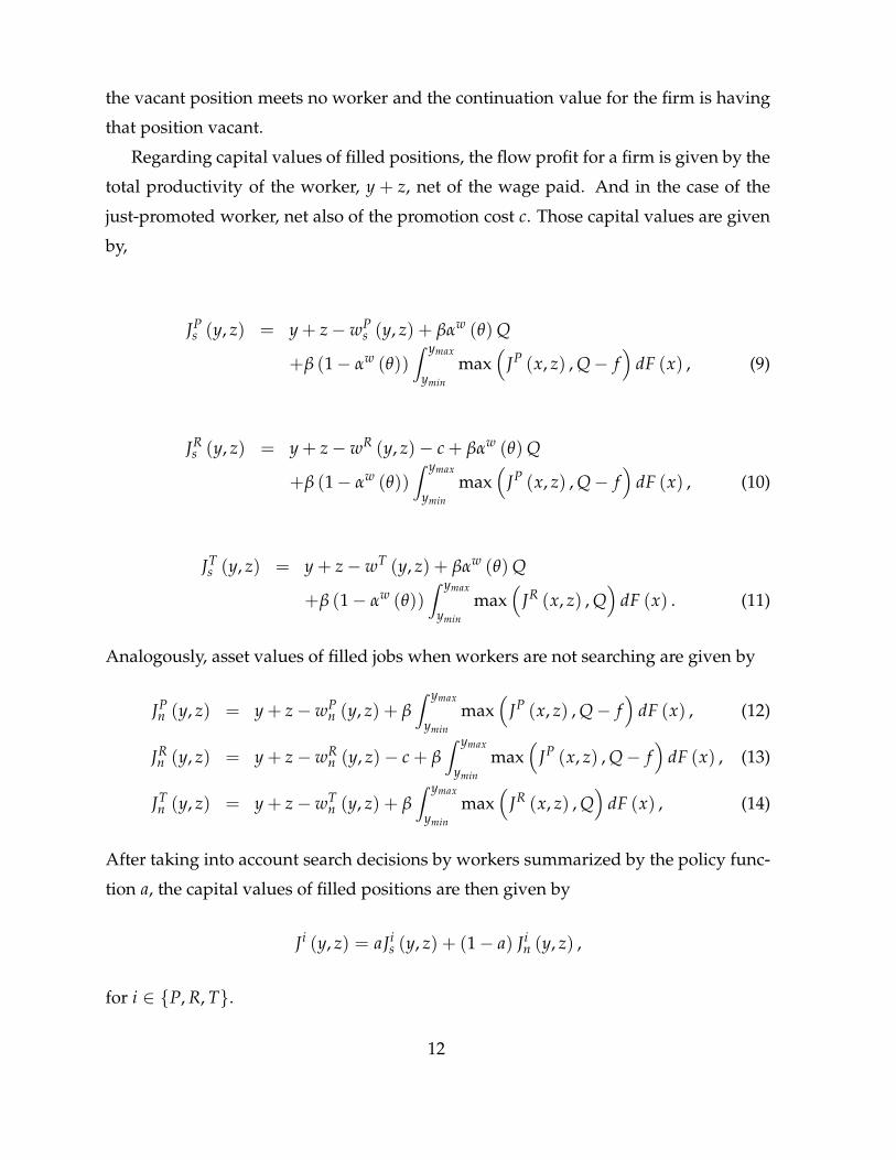
Regarding capital values of filled positions, the flow profit for a firm is given by the

total productivity of the worker, y + z, net of the wage paid. And in the case of the

just-promoted worker, net also of the promotion cost c. Those capital values are given

by,

JPs (y, z) = y + z− wP

s (y, z) + βαw (θ) Q

+β (1− αw (θ))∫ ymax

ymin

max(

JP (x, z) , Q− f)

dF (x) , (9)

JRs (y, z) = y + z− wR (y, z)− c + βαw (θ) Q

+β (1− αw (θ))∫ ymax

ymin

max(

JP (x, z) , Q− f)

dF (x) , (10)

JTs (y, z) = y + z−wT (y, z) + βαw (θ) Q

+β (1− αw (θ))∫ ymax

ymin

max(

JR (x, z) , Q)

dF (x) . (11)

Analogously, asset values of filled jobs when workers are not searching are given by

JPn (y, z) = y + z−wP

n (y, z) + β∫ ymax

ymin

max(

JP (x, z) , Q− f)

dF (x) , (12)

JRn (y, z) = y + z−wR

n (y, z)− c + β∫ ymax

ymin

max(

JP (x, z) , Q− f)

dF (x) , (13)

JTn (y, z) = y + z−wT

n (y, z) + β∫ ymax

ymin

max(

JR (x, z) , Q)

dF (x) , (14)

After taking into account search decisions by workers summarized by the policy func-

tion a, the capital values of filled positions are then given by

Ji (y, z) = aJis (y, z) + (1− a) Ji

n (y, z) ,

for i ∈ {P, R, T}.

12

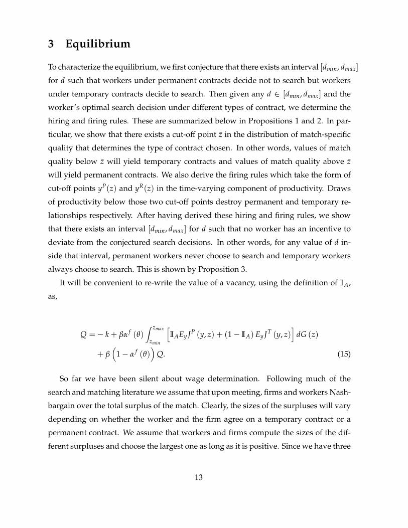
3 Equilibrium

To characterize the equilibrium, we first conjecture that there exists an interval [dmin, dmax]

for d such that workers under permanent contracts decide not to search but workers

under temporary contracts decide to search. Then given any d ∈ [dmin, dmax] and the

worker’s optimal search decision under different types of contract, we determine the

hiring and firing rules. These are summarized below in Propositions 1 and 2. In par-

ticular, we show that there exists a cut-off point z in the distribution of match-specific

quality that determines the type of contract chosen. In other words, values of match

quality below z will yield temporary contracts and values of match quality above z

will yield permanent contracts. We also derive the firing rules which take the form of

cut-off points yP(z) and yR(z) in the time-varying component of productivity. Draws

of productivity below those two cut-off points destroy permanent and temporary re-

lationships respectively. After having derived these hiring and firing rules, we show

that there exists an interval [dmin, dmax] for d such that no worker has an incentive to

deviate from the conjectured search decisions. In other words, for any value of d in-

side that interval, permanent workers never choose to search and temporary workers

always choose to search. This is shown by Proposition 3.

It will be convenient to re-write the value of a vacancy, using the definition of IA,

as,

Q =− k + βα f (θ)∫ zmax

zmin

[

IAEy JP (y, z) + (1− IA) Ey JT (y, z)]

dG (z)

+ β(

1− α f (θ))

Q. (15)

So far we have been silent about wage determination. Following much of the

search and matching literature we assume that upon meeting, firms and workers Nash-

bargain over the total surplus of the match. Clearly, the sizes of the surpluses will vary

depending on whether the worker and the firm agree on a temporary contract or a

permanent contract. We assume that workers and firms compute the sizes of the dif-

ferent surpluses and choose the largest one as long as it is positive. Since we have three

13

different value functions for workers and firms, we have three different surpluses de-

pending on the choices faced by employers and workers.

Denoting by φ the bargaining power of workers, the corresponding total surpluses

for each type of contract are given by:

SP (y, z) = JP (y, z)− (Q− f ) + VP (y, z)−U,

SR (y, z) = JR (y, z)−Q + VR (y, z)−U,

ST (y, z) = JT (y, z)−Q + VT (y, z)−U.

As a result of the bargaining assumption, surpluses satisfy the following splitting

rules:

SP (y, z) =JP (y, z)− Q + f

1− φ=

VP (y, z)−U

φ,

SR (y, z) =JR (y, z)− Q

1− φ=

VR (y, z)−U

φ, (16)

ST (y, z) =JT (y, z)− Q

1− φ=

VT (y, z)−U

φ.

Free entry of firms takes place until any rents associated with vacancy creation are

exhausted, which in turn implies an equilibrium value of a vacancy Q equal to zero.

Replacing Q with its equilibrium value of zero in equation (15) results in the free-entry

condition:

k = βα f (θ)∫ zmax

zmin

[

IAEy JP (y, z) + (1− IA) Ey JT (y, z)]

dG (z)

The interpretation of this equation is that firms expect a per-vacancy-return equal

to the right-hand-side of the expression to justify paying k. Using the surplus sharing

rule in (16) and the free-entry condition, we can derive the following relationship:

∫ zmax

zmin

[

IAEySP (y, z) + (1− IA) EyST (y, z)]

dG (z) =k + βα f (θ) µG (A) f

(1− φ) βα f (θ), (17)

14

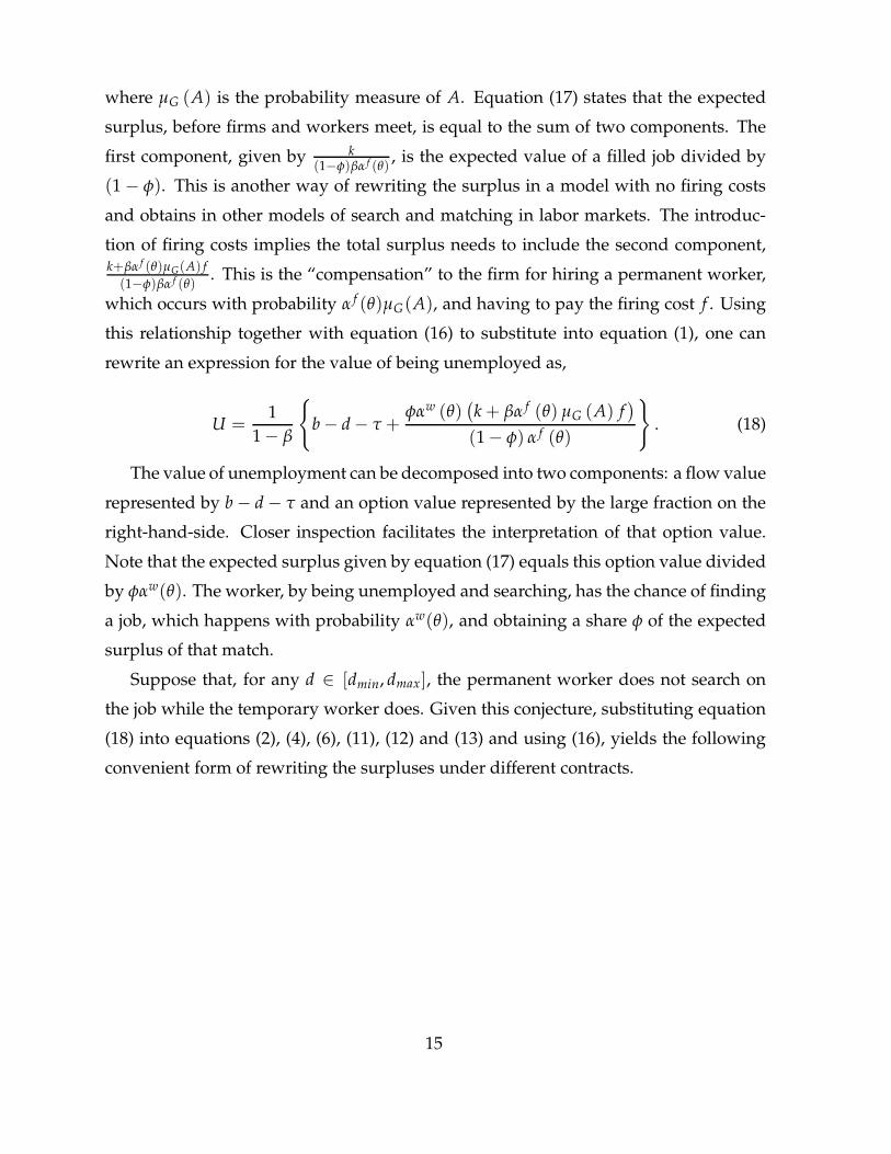
where µG (A) is the probability measure of A. Equation (17) states that the expected

surplus, before firms and workers meet, is equal to the sum of two components. The

first component, given by k(1−φ)βα f (θ)

, is the expected value of a filled job divided by

(1− φ). This is another way of rewriting the surplus in a model with no firing costs

and obtains in other models of search and matching in labor markets. The introduc-

tion of firing costs implies the total surplus needs to include the second component,k+βα f (θ)µG(A) f

(1−φ)βα f (θ). This is the “compensation” to the firm for hiring a permanent worker,

which occurs with probability α f (θ)µG(A), and having to pay the firing cost f . Using

this relationship together with equation (16) to substitute into equation (1), one can

rewrite an expression for the value of being unemployed as,

U =1

1− β

{

b− d− τ +φαw (θ)

(

k + βα f (θ) µG (A) f)

(1− φ) α f (θ)

}

. (18)

The value of unemployment can be decomposed into two components: a flow value

represented by b− d− τ and an option value represented by the large fraction on the

right-hand-side. Closer inspection facilitates the interpretation of that option value.

Note that the expected surplus given by equation (17) equals this option value divided

by φαw(θ). The worker, by being unemployed and searching, has the chance of finding

a job, which happens with probability αw(θ), and obtaining a share φ of the expected

surplus of that match.

Suppose that, for any d ∈ [dmin, dmax], the permanent worker does not search on

the job while the temporary worker does. Given this conjecture, substituting equation

(18) into equations (2), (4), (6), (11), (12) and (13) and using (16), yields the following

convenient form of rewriting the surpluses under different contracts.

15

SP (y, z) = y + z + β∫ ymax

ymin

max(

SP (x, z) , 0)

dF (x) + (1− β) f

− (b− d)−φαw (θ)

(

k + βα f (θ) µG (A) f)

(1− φ) α f (θ), (19)

SR (y, z) = y + z + β∫ ymax

ymin

max(

SP (x, z) , 0)

dF (x)− c− β f

− (b− d)−φαw (θ)

(

k + βα f (θ) µG (A) f)

(1− φ) α f (θ), (20)

ST (y, z) = y + z− b + β (1− αw (θ))∫ ymax

ymin

max(

SR (x, z) , 0)

dF (x) (21)

We begin by deriving the firing rules, by which we mean two threshold produc-

tivity values yP(z) and yR(z). These represent the lowest draws of time-varying pro-

ductivity that imply continuing permanent (yP(z)) or temporary (yR(z)) relationships.

Proposition 1 shows the existence of these values of y, conditional on the type of con-

tract and the specific quality of the match, such that the relationship between a worker

and a firm ends. Before stating that proposition we assume the following:

Assumption 1 Suppose θ is bounded and belongs to [θmin, θmax], i.e., 0 ≤ αw (θmin) <

αw (θmax) ≤ 1 and 0 ≤ α f (θmax) < α f (θmin) ≤ 1. The following inequalities hold for

exogenous parameters:

ymax + zmin ≥ b− dmin +φ

1− φ(θmaxk + βαw (θmax) f )− (1− β) f , (22)

b− dmax +φ

1− φθmink− (1− β) f ≥ ymin + zmax + β

∫ ymax

ymin

(1− F (x)) dx (23)

Assumption 2 In addition,

ymax + zmin − c− f ≥ b− dmin +φ

1− φ(θmaxk + βαw (θmax) f )− (1− β) f . (24)

Proposition 1 Under Assumption 1, for any d ∈ [dmin, dmax] and any z, there exists an

unique cut-off value yP (z) ∈ (ymin, ymax) and such that SP(

yP (z) , z)

= 0. If Assumption 2

also holds then the unique cut-off value yR (z) ∈ (ymin, ymax) exists where SR(

yR (z) , z)

= 0.

16

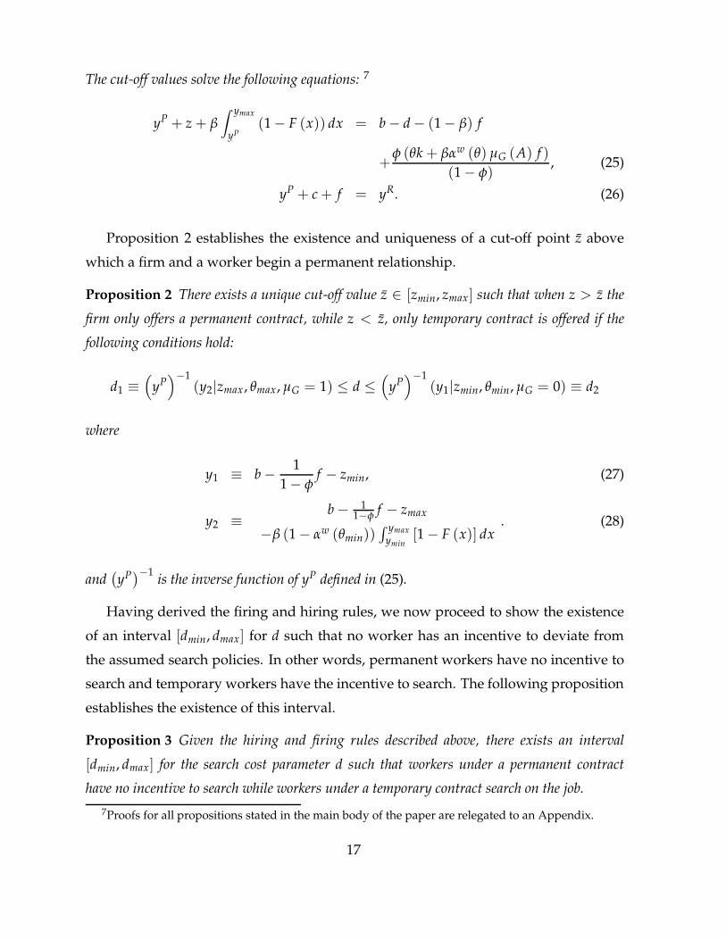
The cut-off values solve the following equations: 7

yP + z + β∫ ymax

yP(1− F (x)) dx = b− d− (1− β) f

+φ (θk + βαw (θ) µG (A) f )

(1− φ), (25)

yP + c + f = yR. (26)

Proposition 2 establishes the existence and uniqueness of a cut-off point z above

which a firm and a worker begin a permanent relationship.

Proposition 2 There exists a unique cut-off value z ∈ [zmin, zmax] such that when z > z the

firm only offers a permanent contract, while z < z, only temporary contract is offered if the

following conditions hold:

d1 ≡(

yP)−1

(y2|zmax , θmax, µG = 1) ≤ d ≤(

yP)−1

(y1|zmin, θmin, µG = 0) ≡ d2

where

y1 ≡ b−1

1− φf − zmin, (27)

y2 ≡b− 1

1−φ f − zmax

−β (1− αw (θmin))∫ ymax

ymin[1− F (x)] dx

. (28)

and(

yP)−1

is the inverse function of yP defined in (25).

Having derived the firing and hiring rules, we now proceed to show the existence

of an interval [dmin, dmax] for d such that no worker has an incentive to deviate from

the assumed search policies. In other words, permanent workers have no incentive to

search and temporary workers have the incentive to search. The following proposition

establishes the existence of this interval.

Proposition 3 Given the hiring and firing rules described above, there exists an interval

[dmin, dmax] for the search cost parameter d such that workers under a permanent contract

have no incentive to search while workers under a temporary contract search on the job.

7Proofs for all propositions stated in the main body of the paper are relegated to an Appendix.

17

The existence of the interval defined in Proposition 3 should be intuitive to the reader.

If on-the-job search is too costly no employed worker would search irrespective of the

type of contract. Likewise, if search costs little all workers might opt to seek alternative

employment opportunities. However, it is also intuitive that for a given value of d, on-

the-job search is more costly for workers under high-quality matches. The reason is

that the “return” of searching on the job is lower for those high match-quality workers.

These are precisely the workers hired under permanent contracts, and as a result there

is a region for the on-the-job search cost d such that permanent workers do not search

but temporary workers do.

To obtain expressions for wages paid under different contracts we can substitute the

value functions of workers and firms into the surplus sharing rule (16), which gives:

wP (y, z) = φ (y + z) + (1− φ) (b− d)

+φ

[

(1− β) f +αw (θ)

α f (θ)

(

k + βα f (θ) µG (A) f)

]

, (29)

wR (y, z) = wP (y, z)− φ (c + f ) , (30)

wT (y, z) = φ (y + z) + (1− φ) b. (31)

Finally, we need to explicitly state how the stock of employment evolves over time.

Let ut denote the measure of unemployment, and nPt and nT

t be the measure of perma-

nent workers and temporary workers. Let’s begin by deriving the law of motion of the

stock of permanent workers, which is given by the sum of three groups of workers.

First, unemployed workers and temporary workers can search and match with other

firms and become permanent workers. This happens with probability αw (θt) µG (A).

Second, after the realization of the aggregate shock, the permanent worker remains at

the current job. The aggregate quantity of this case is∫ zmax

zminµF

([

yP (z) , ymax

])

dG (z) nPt .

Third, some of temporary workers who cannot find other jobs get promoted to perma-

nent workers which adds to the aggregate employment pool for permanent workers

by (1− αw (θt))∫ z

zminµF

([

yR (z) , ymax

])

dG (z) nTt . Notice that µG (A) = 1− G (z) and

18

µF ([y, ymax]) = 1− F (y). The law of motion for permanent workers becomes:

nPt+1 =

(

ut + nTt

)

αw (θt) (1− G (z)) +∫ zmax

zmin

[

1− F(

yP (z))]

dG (z) nPt

+ (1− αw (θt))1

G(z)

∫ z

zmin

[

1− F(

yR (z))]

dG (z) nTt . (32)

Unemployed workers and temporary workers who are unable to find high-quality

matches, join the temporary worker pool the following period. Therefore the tem-

porary workers evolve according to:

nTt+1 =

(

ut + nTt

)

αw (θt) G (z) . (33)

Since the aggregate population is normalized to unity, the mass of unemployed work-

ers is given by:

ut = 1− nTt − nP

t .

The standard definition of market tightness is slightly modified to account for the on-

the-job search activity of temporary workers:

θt =vt

ut + nTt

.

4 Partial Equilibrium Analysis

To understand the intuition behind some of the results we show in the quantitative sec-

tion, we perform here some comparative statics in “partial” equilibrium, by which we

mean keeping θ constant. The goal is to understand how changes in selected variables

impact the hiring and firing decisions.

Proposition 4 The hiring rule has the following properties:

1. dz/d f > 0,

2.

dz/dαw< 0 when φ < φ

dz/dαw> 0 when φ > φ

,

19

3. dz/dc < 0.

The intuition behind Proposition 4 can be illustrated in Figures 1 to 3 . Figure 1

shows the effects of an increase in the firing cost f . This increase has two effects on the

(net) value of a filled job.8 The direct effect causes a drop in the value of a permanent

job because the firm has to pay more to separate from the worker. As a result the

permanent contract curve shifts downward. An increase in f also increases the job

destruction rate of temporary workers by raising the threshold value yR, lowering the

value of a temporary job. In equilibrium, the first effect dominates resulting in fewer

permanent contracts.

Increasing the job finding probability has an ambiguous effect on the hiring deci-

sion because it depends on the worker’s bargaining power. If it is easier for unem-

ployed workers to find a job, the value of being unemployed increases because the

unemployment spell is shortened. This lowers the match surplus since the worker’s

outside option rises. Therefore, the value of filled jobs falls and (both permanent and

temporary) contract curves shifts outward. We call this the unemployment effect. How-

ever, there are two additional effects on temporary jobs. Since the temporary worker

searches on-the-job, the higher job finding probability increases the chance that a tem-

porary worker remains employed. Therefore, the match surplus rises due to the in-

crease in the value of temporary employment. We call this effect the job continuation

effect. For workers under temporary contract, these two effects exactly cancel out. On

the other hand, the higher job finding probability causes more separations of tempo-

rary contracts. This so-called job turnover effect reduces the value of a temporary job

which moves the temporary contract curve outward. If a worker has more bargain-

ing power, then the unemployment effect dominates the job turnover effect. This case

is depicted in Figure 1. However if the worker’s bargaining power is small, the job

turnover effect dominates the unemployment effect which leads to fewer temporary

workers. The latter case is shown in Figure 2.

8The size of the surplus determines the type of contract chosen or whether matches continue orare destroyed. By Nash bargaining the value of a filled job is proportional to the total surplus, so itis sufficient to compare the changes in the values of filled jobs to determine the effects on the totalsurpluses.

20

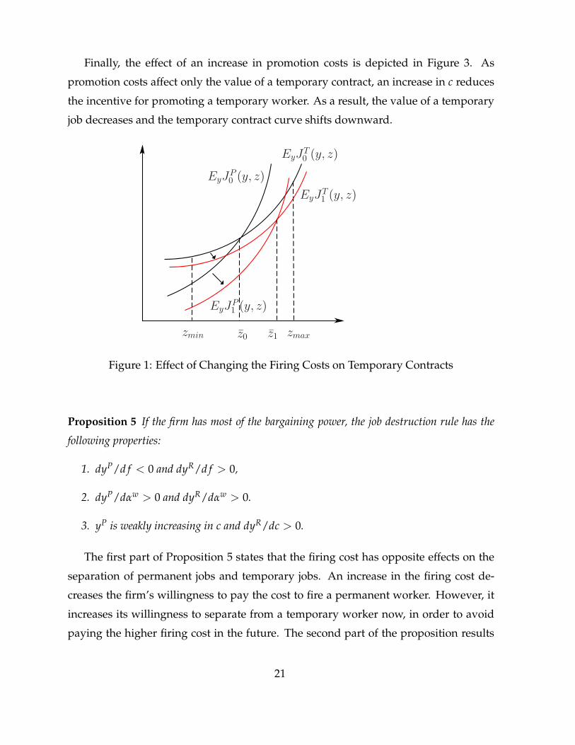
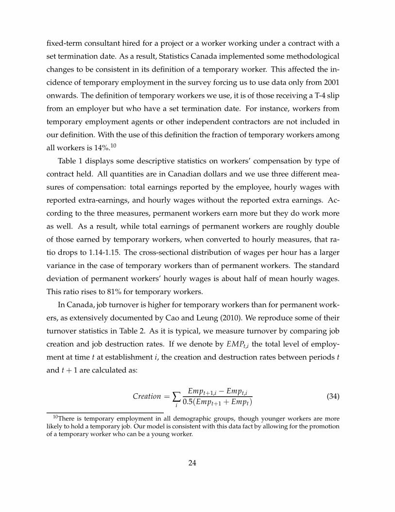
Finally, the effect of an increase in promotion costs is depicted in Figure 3. As

promotion costs affect only the value of a temporary contract, an increase in c reduces

the incentive for promoting a temporary worker. As a result, the value of a temporary

job decreases and the temporary contract curve shifts downward.

zmin z0 zmax

EyJP0(y, z)

EyJT0(y, z)

z1

EyJP1(y, z)

EyJT1(y, z)

Figure 1: Effect of Changing the Firing Costs on Temporary Contracts

Proposition 5 If the firm has most of the bargaining power, the job destruction rule has the

following properties:

1. dyP/d f < 0 and dyR/d f > 0,

2. dyP/dαw> 0 and dyR/dαw

> 0.

3. yP is weakly increasing in c and dyR/dc > 0.

The first part of Proposition 5 states that the firing cost has opposite effects on the

separation of permanent jobs and temporary jobs. An increase in the firing cost de-

creases the firm’s willingness to pay the cost to fire a permanent worker. However, it

increases its willingness to separate from a temporary worker now, in order to avoid

paying the higher firing cost in the future. The second part of the proposition results

21

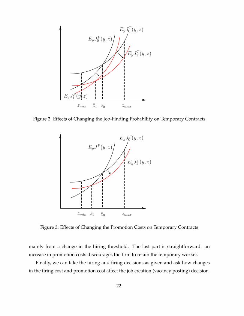
zmin z0 zmax

EyJP0(y, z)

EyJT0(y, z)

z1

EyJP1(y, z)

EyJT1(y, z)

Figure 2: Effects of Changing the Job-Finding Probability on Temporary Contracts

zmin z0 zmax

EyJP (y, z)

EyJT0(y, z)

z1

EyJT1(y, z)

Figure 3: Effects of Changing the Promotion Costs on Temporary Contracts

mainly from a change in the hiring threshold. The last part is straightforward: an

increase in promotion costs discourages the firm to retain the temporary worker.

Finally, we can take the hiring and firing decisions as given and ask how changes

in the firing cost and promotion cost affect the job creation (vacancy posting) decision.

22

The following proposition summarizes the results.

Proposition 6 Given the hiring and permanent job destruction rules, i.e. z and yP (z) are

fixed, dθ/d f < 0 if β is not too small and dθ/dc < 0.

The explanation of this proposition is that an increase in firing costs and promotion

costs discourages the firm to post more vacancies by reducing the expected profits of

jobs.

5 Data

To quantitatively explore the model, we use the Workplace and Employee Survey, a

Canadian matched employer-employee dataset collected by Statistics Canada. It is

an annual, longitudinal survey at the establishment level, targeting establishments in

Canada that have paid employees in March, with the exceptions of those operating in

the crop and animal production; fishing, hunting and trapping; households’, religious

organizations, and the government sectors. In 1999, it consisted of a sample of 6,322

establishments drawn from the Business Register maintained by Statistics Canada and

the sample has been followed ever since. Every odd year the sample has been aug-

mented with newborn establishments that have become part of the Business Register.

The data are rich enough to allow us to distinguish employees by the type of contract

they hold. However, only a sample of employees is surveyed from each establishment.9 The average number of employees in the sample is roughly 20,000 each year. Work-

ers are followed for two years and provide responses on hours worked, earnings, job

history, education, and demographic information. Firms provide information about

hiring conditions of different workers, payroll and other compensation, vacancies, and

separation of workers.

Given the theory laid out above, it is important that the definition of temporary

worker in the data matches as close as possible the concept of a temporary worker in

the model. In principle, it is unclear that all establishments share the idea of what a

temporary worker is when they respond to the survey: it could be a seasonal worker, a

9All establishments with less than four employees are surveyed. In larger establishments, a sampleof workers is surveyed, with a maximum of 24 employees per given establishment.

23

fixed-term consultant hired for a project or a worker working under a contract with a

set termination date. As a result, Statistics Canada implemented some methodological

changes to be consistent in its definition of a temporary worker. This affected the in-

cidence of temporary employment in the survey forcing us to use data only from 2001

onwards. The definition of temporary workers we use, it is of those receiving a T-4 slip

from an employer but who have a set termination date. For instance, workers from

temporary employment agents or other independent contractors are not included in

our definition. With the use of this definition the fraction of temporary workers among

all workers is 14%.10

Table 1 displays some descriptive statistics on workers’ compensation by type of

contract held. All quantities are in Canadian dollars and we use three different mea-

sures of compensation: total earnings reported by the employee, hourly wages with

reported extra-earnings, and hourly wages without the reported extra earnings. Ac-

cording to the three measures, permanent workers earn more but they do work more

as well. As a result, while total earnings of permanent workers are roughly double

of those earned by temporary workers, when converted to hourly measures, that ra-

tio drops to 1.14-1.15. The cross-sectional distribution of wages per hour has a larger

variance in the case of temporary workers than of permanent workers. The standard

deviation of permanent workers’ hourly wages is about half of mean hourly wages.

This ratio rises to 81% for temporary workers.

In Canada, job turnover is higher for temporary workers than for permanent work-

ers, as extensively documented by Cao and Leung (2010). We reproduce some of their

turnover statistics in Table 2. As it is typical, we measure turnover by comparing job

creation and job destruction rates. If we denote by EMPt,i the total level of employ-

ment at time t at establishment i, the creation and destruction rates between periods t

and t + 1 are calculated as:

Creation = ∑i

Empt+1,i − Empt,i

0.5(Empt+1 + Empt)(34)

10There is temporary employment in all demographic groups, though younger workers are morelikely to hold a temporary job. Our model is consistent with this data fact by allowing for the promotionof a temporary worker who can be a young worker.

24

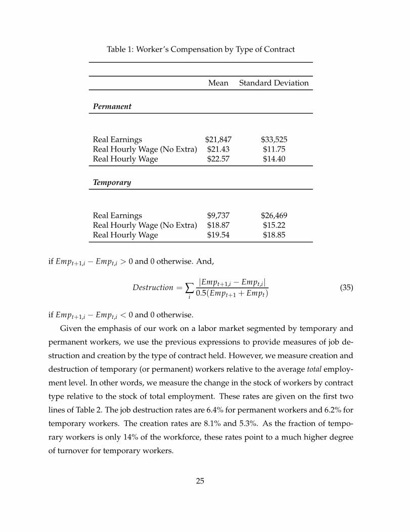
Table 1: Worker’s Compensation by Type of Contract

Mean Standard Deviation

Permanent

Real Earnings $21,847 $33,525Real Hourly Wage (No Extra) $21.43 $11.75Real Hourly Wage $22.57 $14.40

Temporary

Real Earnings $9,737 $26,469Real Hourly Wage (No Extra) $18.87 $15.22Real Hourly Wage $19.54 $18.85

if Empt+1,i − Empt,i > 0 and 0 otherwise. And,

Destruction = ∑i

|Empt+1,i − Empt,i|

0.5(Empt+1 + Empt)(35)

if Empt+1,i − Empt,i < 0 and 0 otherwise.

Given the emphasis of our work on a labor market segmented by temporary and

permanent workers, we use the previous expressions to provide measures of job de-

struction and creation by the type of contract held. However, we measure creation and

destruction of temporary (or permanent) workers relative to the average total employ-

ment level. In other words, we measure the change in the stock of workers by contract

type relative to the stock of total employment. These rates are given on the first two

lines of Table 2. The job destruction rates are 6.4% for permanent workers and 6.2% for

temporary workers. The creation rates are 8.1% and 5.3%. As the fraction of tempo-

rary workers is only 14% of the workforce, these rates point to a much higher degree

of turnover for temporary workers.

25

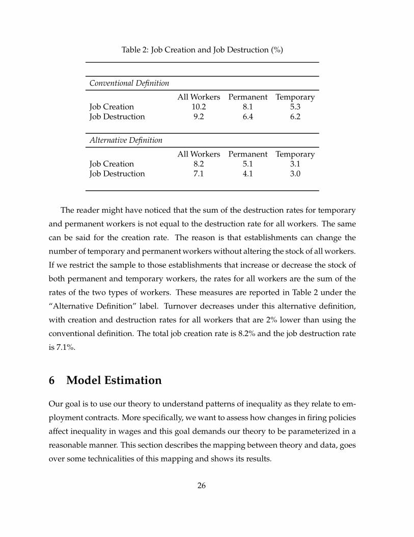
Table 2: Job Creation and Job Destruction (%)

Conventional Definition

All Workers Permanent TemporaryJob Creation 10.2 8.1 5.3Job Destruction 9.2 6.4 6.2

Alternative Definition

All Workers Permanent TemporaryJob Creation 8.2 5.1 3.1Job Destruction 7.1 4.1 3.0

The reader might have noticed that the sum of the destruction rates for temporary

and permanent workers is not equal to the destruction rate for all workers. The same

can be said for the creation rate. The reason is that establishments can change the

number of temporary and permanent workers without altering the stock of all workers.

If we restrict the sample to those establishments that increase or decrease the stock of

both permanent and temporary workers, the rates for all workers are the sum of the

rates of the two types of workers. These measures are reported in Table 2 under the

“Alternative Definition” label. Turnover decreases under this alternative definition,

with creation and destruction rates for all workers that are 2% lower than using the

conventional definition. The total job creation rate is 8.2% and the job destruction rate

is 7.1%.

6 Model Estimation

Our goal is to use our theory to understand patterns of inequality as they relate to em-

ployment contracts. More specifically, we want to assess how changes in firing policies

affect inequality in wages and this goal demands our theory to be parameterized in a

reasonable manner. This section describes the mapping between theory and data, goes

over some technicalities of this mapping and shows its results.

26

Obtaining a solution for the model requires specifying parametric distributions for

G(z) and F(y).11 We assume that y is drawn from a normal distribution and z from a

uniform distribution. In the model the overall scale of the economy is indeterminate

and shifts in the mean of y plus z have no impact. Consequently, we normalize the

mean of y plus z to one, reducing the dimension of the parameter vector of interest.

One needs a functional form for the matching technology as well. Denote by B the

level of matches given vacancies v and searching workers NS = nT + u. Note that

we have already excluded the mass of permanent workers from the pool of search-

ing workers. Given that our data set does not provide information about on the job

behavior (or job-to-job transitions), we fix d to a value of zero and check whether the

sufficient conditions of Proposition 3 hold. With this fixed value for d we estimate the

remaining parameters of interest. We give more detail a few paragraphs below on how

we perform that estimation. But first, we assume the matching function to be of the

form,

B(v, NS) =vNS

(vξ + NSξ)

1ξ

.

This choice of technology for the matching process implies the following job-finding

and job-filling rates, where, again we define θ = v/NS:

αw(θ) =θ

(1 + θξ)1ξ

,

and

α f (θ) =1

(1 + θξ)1ξ

.

Having specified parametric forms for G, F, and the matching technology we are

now ready to describe our procedure in detail. Let γ = ( f , b, φ, ξ, k, µy , σz, σy) be the

vector of structural parameters we need to estimate where µx and σx denote the mean

and the standard deviation for a random variable x.12 The literature estimating search

11The reader can find much technical detail about our solution and estimation algorithms in a Techni-cal Appendix

12Parameters c, β, and µz, should in principle be included in the vector γ. We fix β to be 0.96 and c tobe 1% of the firing cost f . The standard deviation of z is given by the normalization that E(y) + E(z) = 1.

27

models is large and much of it has followed full-information estimation methodolo-

gies, maximizing a likelihood function of histories of workers.13 These workers face

exogenous arrival rates of job offers (both on and off-the-job) and choose to accept or

reject such offers. Parameters maximize the likelihood of observing workers’ histories

conditional on the model’s decision rules. In this paper, we depart from this literature

by choosing a partial information approach to estimating our model. Our reason is

twofold. First, our search model is an equilibrium one; the arrival rates of job offers

are the result of aggregate behavior from the part of consumers and firms. Second, the

lack of a panel dimension of the WES does not allow us to perform a maximum like-

lihood estimation. For these reasons, we take a partial-information route and estimate

the model by combining indirect inference and simulated method of moments.

The first step involves choosing a set of empirical moments; set of dimension at least

as large as the parameter vector of interest. We estimate the parameters by minimizing

a quadratic function of the deviations of those empirical moments from their model-

simulated counterparts. Formally,

γ = argminγ

M(γ, YT)′W(γ, YT)M(γ, YT) (36)

where γ denotes the point estimate for γ, W is a weighting matrix, and M is a

column vector whose k-th element denotes a deviation of an empirical moment and a

model-simulated moment. The vector YT describes time series data - of length T - from

which we compute the empirical moments. The above expression should be familiar

to readers, as it is a standard statistical criterion function in the method-of-moments or

GMM literatures. Traditional estimation techniques rely on minimizing the criterion

function (36) and using the Hessian matrix evaluated at the minimized value to com-

pute standard errors. In many instances equation (36) is non-smooth, locally flat, and

have several local minima. For these reasons, we use the quasi-Bayesian Laplace Type

Estimator (LTE) proposed by Chernozhukov and Hong (2003). They show that un-

der some technical assumptions, a transformation of (36) is a proper density function

13The list is far from being exhaustive but it includes Cahuc et al. (2006), Finn and Mabli (2009),Bontemps et al. (1999), Eckstein and Wolpin (1990). The reader is referred to Eckstein and Van den Berg(2007) for a survey of the literature that includes many more examples.

28

(in their language, a quasi-posterior density function) As a result, they show how mo-

ments of interest can be computed using using Markov Chain Monte Carlo (MCMC)

techniques by sampling from that quasi-posterior density. We describe our estimation

technique in more detail in the technical appendix, but MCMC essentially amounts to

constructing a Markov chain that converges to the density function implied by a trans-

formation of (36). Draws from that Markov Chain are draws from the quasi-posterior,

and as a result, moments of the parameter vector such as means, standard deviations,

or othe quantities of interest are readily available. An important aspect of the estima-

tion procedure is the choice of the weighting matrix W. We post-pone a description

of how we weight the different moments and we now turn to describe the moments

themselves.

Indirect inference involves positing an auxiliary - reduced-form - model which links

actual data and model-simulated data. Given our focus on wage inequality, the aux-

iliary model we choose is a wage regression that links wages, productivity, and the

type of contract held. Before being more specific about this regression let us first dis-

cuss an identification assumption needed to estimate it. An important element in our

model’s solution are wages by type of contract which are given by equations (29)-

(31). Irrespective of the type of contract wages are always a function of a worker’s

productivity y + z. In the data, such productivity is unobserved; one observes an es-

tablishment’s total productivity or the productivity for the entire sample. To overcome

this difficulty we assume that the time-varying component of productivity y is firm

or establishment-specific. Consequently, differences among workers’ wages within a

firm will be the result of working under a different contract or of having a different

match-specific quality. We then posit that the (log) wage of worker i of firm j at time t

is given by:

log(wijt) = β + βALPlog(ALPjt) + βTypeχijt + ǫijt (37)

where ALPjt is an establishment’s average labor productivity - output divided by

total hours - and χijt is an indicator variable describing a worker’s temporary status.

This is the equation we estimate from the data.14 A panel of values for ALPjt is easy to

14We take logarithms for wages and ALPjt as our model is stationary and displays no productivity

29

obtain, as we have observations on the number of workers and the amount of output

per establishment. Note that variations over time in ALPjt arise from changes in the

time-varying productivity shock but also from the matches and separations that occur

within a establishment over time. If as a result of turnover within a establishment, the

mix of workers changes- there are more temporary workers in some year, for instance-

the average worker productivity will change, even without a change in yjt. Let us now

describe what is the analogous equation to (37) we estimate in our model-simulated

data. Our theory is silent about firms or establishments; there are only matches of

which one can reasonably speak. Note, however, that ALPjt is the sum of the time-

varying component yjt plus an expectation of the match-specific productivity z at time

t - assuming a large number of workers per establishment. Hence, we simulate a large

number of values of y, z, and wages by contract type and regress the logarithm of

wages on a constant, the logarithm of the sum of y and the mean simulated z and the

contract type. Disturbances in this regression will be interpreted as deviations of the

match-specific quality for a given match relative to its mean match-specific value (plus

some small degree of simulation error).

Our sample of the WES data-set covers the years 2001 to 2006. We estimate equation

(37) for each year which yields a series of estimates (β, βALP, βType, σǫ). Returning to

our criterion function (36), the first two moments we choose to match are the time-

series averages of the coefficients βALP and βType. Table 3 summarizes the vector of all

moments (a total of 13), which includes time-series averages of job-creation and job-

destruction (for all workers, JD and JC; and for permanent and temporary workers,

JCP, JDP, JCT, and JDT)15, the fraction of temporary workers ( nT

1−u ), the job-finding

probability (αw), and the ratio of wages of permanent workers to those of temporary

workers (wP

wT ), the unemployment rate (u), and the average of the fraction of the firing

costs relative to the wage of a permanent worker ( fwP ).16

The deviations of the empirical averages from their model counterparts comprise

the vector M. Following much of the GMM literature, we weight elements of M accord-

growth.15We follow the “Conventional Definition” (see Table 2) for computing these destruction and creation

rates. In the Appendix the reader will find detailed expressions that show how we calculate them.16We thank M. Zhang for sharing her data on the Canadian job-finding rate used in Zhang (2008).

30

Table 3: Statistical Properties: Empirical Moments (2001-2006)

Series Mean StandardDeviation

JD 0.092 0.025JC 0.102 0.018JDP 0.064 0.020JDT 0.062 0.015JCP 0.081 0.021JCT 0.053 0.009nT/(1− u) 0.140 0.040αw 0.919 0.004f /wP 0.182 0.002wP/wT 1.140 0.034u 0.071 0.004βAPL 0.159 0.013βType 0.193 0.019

ing to the inverse of the covariance matrix of the deviations of the time series shown

in Table 3 from their model equivalents.

7 Results

Table 4 shows the estimated parameter values along with their standard errors. The

point estimates are the quasi-posterior means and the standard errors are the quasi-

posterior standard deviations.17 We estimate a bargaining power of workers φ equal

to 0.62. This value is about the same magnitude as those that are calibrated, but larger

than previously estimated values such as Cahuc et al.’s (2006), which is very close to

zero. The estimation yields distributions for y and z whose means are far apart. Recall

that E(y) + E(z) = 1 but E(y) is larger than 4. The theory imposes several restrictions

on the parameter vector beyond the usual ones (e.g. φ ∈ (0, 1)). In particular, we

impose the restrictions over the parameter space described in Assumptions 1 and 2,

and also those sufficient restrictions for the results we present in Proposition 2 to be

17These results are based on 4,000 draws of the Markov chain.

31

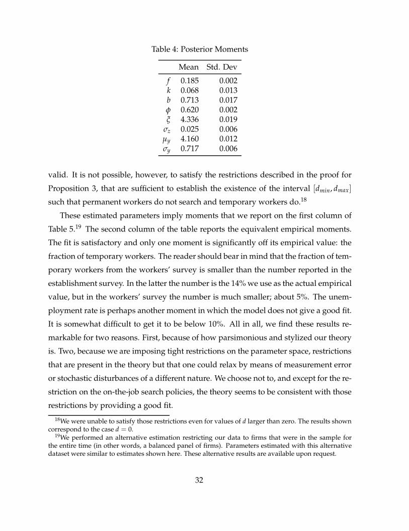
Table 4: Posterior Moments

Mean Std. Dev

f 0.185 0.002k 0.068 0.013b 0.713 0.017φ 0.620 0.002ξ 4.336 0.019

σz 0.025 0.006µy 4.160 0.012σy 0.717 0.006

valid. It is not possible, however, to satisfy the restrictions described in the proof for

Proposition 3, that are sufficient to establish the existence of the interval [dmin, dmax]

such that permanent workers do not search and temporary workers do.18

These estimated parameters imply moments that we report on the first column of

Table 5.19 The second column of the table reports the equivalent empirical moments.

The fit is satisfactory and only one moment is significantly off its empirical value: the

fraction of temporary workers. The reader should bear in mind that the fraction of tem-

porary workers from the workers’ survey is smaller than the number reported in the

establishment survey. In the latter the number is the 14% we use as the actual empirical

value, but in the workers’ survey the number is much smaller; about 5%. The unem-

ployment rate is perhaps another moment in which the model does not give a good fit.

It is somewhat difficult to get it to be below 10%. All in all, we find these results re-

markable for two reasons. First, because of how parsimonious and stylized our theory

is. Two, because we are imposing tight restrictions on the parameter space, restrictions

that are present in the theory but that one could relax by means of measurement error

or stochastic disturbances of a different nature. We choose not to, and except for the re-

striction on the on-the-job search policies, the theory seems to be consistent with those

restrictions by providing a good fit.

18We were unable to satisfy those restrictions even for values of d larger than zero. The results showncorrespond to the case d = 0.

19We performed an alternative estimation restricting our data to firms that were in the sample forthe entire time (in other words, a balanced panel of firms). Parameters estimated with this alternativedataset were similar to estimates shown here. These alternative results are available upon request.

32

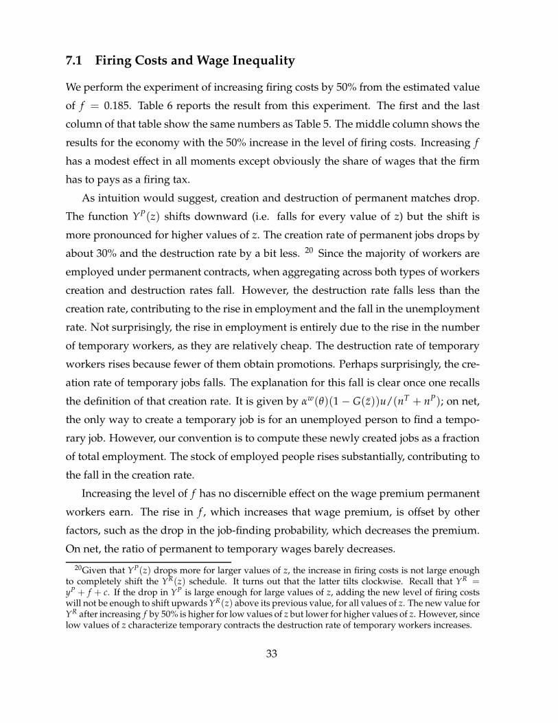
7.1 Firing Costs and Wage Inequality

We perform the experiment of increasing firing costs by 50% from the estimated value

of f = 0.185. Table 6 reports the result from this experiment. The first and the last

column of that table show the same numbers as Table 5. The middle column shows the

results for the economy with the 50% increase in the level of firing costs. Increasing f

has a modest effect in all moments except obviously the share of wages that the firm

has to pays as a firing tax.

As intuition would suggest, creation and destruction of permanent matches drop.

The function YP(z) shifts downward (i.e. falls for every value of z) but the shift is

more pronounced for higher values of z. The creation rate of permanent jobs drops by

about 30% and the destruction rate by a bit less. 20 Since the majority of workers are

employed under permanent contracts, when aggregating across both types of workers

creation and destruction rates fall. However, the destruction rate falls less than the

creation rate, contributing to the rise in employment and the fall in the unemployment

rate. Not surprisingly, the rise in employment is entirely due to the rise in the number

of temporary workers, as they are relatively cheap. The destruction rate of temporary

workers rises because fewer of them obtain promotions. Perhaps surprisingly, the cre-

ation rate of temporary jobs falls. The explanation for this fall is clear once one recalls

the definition of that creation rate. It is given by αw(θ)(1− G(z))u/(nT + nP); on net,

the only way to create a temporary job is for an unemployed person to find a tempo-

rary job. However, our convention is to compute these newly created jobs as a fraction

of total employment. The stock of employed people rises substantially, contributing to

the fall in the creation rate.

Increasing the level of f has no discernible effect on the wage premium permanent

workers earn. The rise in f , which increases that wage premium, is offset by other

factors, such as the drop in the job-finding probability, which decreases the premium.

On net, the ratio of permanent to temporary wages barely decreases.

20Given that YP(z) drops more for larger values of z, the increase in firing costs is not large enoughto completely shift the YR(z) schedule. It turns out that the latter tilts clockwise. Recall that YR =yP + f + c. If the drop in YP is large enough for large values of z, adding the new level of firing costswill not be enough to shift upwards YR(z) above its previous value, for all values of z. The new value forYR after increasing f by 50% is higher for low values of z but lower for higher values of z. However, sincelow values of z characterize temporary contracts the destruction rate of temporary workers increases.

33

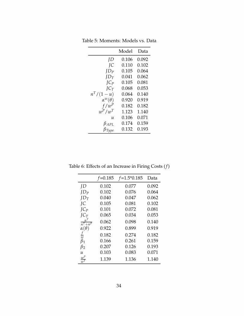
Table 5: Moments: Models vs. Data

Model Data

JD 0.106 0.092JC 0.110 0.102

JDP 0.105 0.064JDT 0.041 0.062JCP 0.105 0.081JCT 0.068 0.053

nT/(1− u) 0.064 0.140αw(θ) 0.920 0.919f /wP 0.182 0.182

wP/wT 1.123 1.140u 0.106 0.071

βAPL 0.174 0.159βType 0.132 0.193

Table 6: Effects of an Increase in Firing Costs ( f )

f =0.185 f =1.5*0.185 Data

JD 0.102 0.077 0.092JDP 0.102 0.076 0.064JDT 0.040 0.047 0.062JC 0.105 0.081 0.102JCP 0.101 0.072 0.081JCT 0.065 0.034 0.053

nT

nT+nP 0.062 0.098 0.140α(θ) 0.922 0.899 0.919fw 0.182 0.274 0.182β1 0.166 0.261 0.159β2 0.207 0.126 0.193u 0.103 0.083 0.071wP

wT 1.139 1.136 1.140

34

What are the implications of these changes for the shape of the wage distribution?

Figure 4 shows the wage distribution for the three cases discussed. The blue (solid) line

represents the density function of wages (using standard kernel-smoothing methods)

when the parameters are set to their quasi-posterior means. If we increase the level of

firing costs by 50%, the result is the red (dashed-dotted) line: lower mean wages, be-

cause of the larger fraction of temporary workers, and considerably larger inequality.21

0 0.2 0.4 0.6 0.8 1 1.2 1.4 1.6 1.80

0.2

0.4

0.6

0.8

1

1.2

1.4

1.6

1.8

2Firing Costs and the Wage Distribution

w

f(w

)

Baseline1.5*f

Figure 4: Wage distributions for different levels of firing costs.

7.2 The Welfare Implications of Temporary Contracts

We now provide some calculations of the changes in welfare that result from the intro-

duction of temporary contracts in economies where existing workers are protected by

firing costs. We do so by performing the following computational experiment. Given

the estimated parameters above (the baseline case), we force z to drop to a level in

21Inequality measured using the standard deviation rises by 21% and the mean of wages falls byroughly 6%.

35

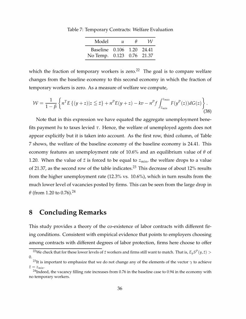
Table 7: Temporary Contracts: Welfare Evaluation

Model u θ W

Baseline 0.106 1.20 24.41No Temp. 0.123 0.76 21.37

which the fraction of temporary workers is zero.22 The goal is to compare welfare

changes from the baseline economy to this second economy in which the fraction of

temporary workers is zero. As a measure of welfare we compute,

W =1

1− β

{

nTE {(y + z)|z ≦ z}+ nPE(y + z)− kv− nP f∫ zmax

zmin

F(yP(z))dG(z)

}

.

(38)

Note that in this expression we have equated the aggregate unemployment bene-

fits payment bu to taxes levied τ. Hence, the welfare of unemployed agents does not

appear explicitly but it is taken into account. As the first row, third column, of Table

7 shows, the welfare of the baseline economy of the baseline economy is 24.41. This

economy features an unemployment rate of 10.6% and an equilibrium value of θ of

1.20. When the value of z is forced to be equal to zmin, the welfare drops to a value

of 21.37, as the second row of the table indicates.23 This decrease of about 12% results

from the higher unemployment rate (12.3% vs. 10.6%), which in turn results from the

much lower level of vacancies posted by firms. This can be seen from the large drop in

θ (from 1.20 to 0.76).24

8 Concluding Remarks

This study provides a theory of the co-existence of labor contracts with different fir-

ing conditions. Consistent with empirical evidence that points to employers choosing

among contracts with different degrees of labor protection, firms here choose to offer

22We check that for these lower levels of z workers and firms still want to match. That is, EySP(y, z) >0.

23It is important to emphasize that we do not change any of the elements of the vector γ to achievez = zmin.

24Indeed, the vacancy filling rate increases from 0.76 in the baseline case to 0.94 in the economy withno temporary workers.

36

ex-ante identical workers different contracts, and as a result, different wages. The rea-

son is match-quality that varies across worker-firm pairs and that is revealed at the

moment firms and workers meet. Firms offer permanent contracts to “good” matches,

as they risk losing the worker should they offer them a temporary contract. This risk

results from the different on-the-job search behavior by the two types of workers: in

equilibrium temporary workers search while permanent workers do not. Not-so-good

matches are given a temporary contract under which they work for a lower wage. Af-

ter one period, temporary workers have to be dismissed or promoted to permanent

status.

The existence of search and matching frictions implies that workers might work

temporarily in jobs with an inferior match quality, before transferring to better, and

more stable, matches. Our assumption of including a time-varying component in the

total productivity of a worker allows our environment to generate endogenous de-

struction rates that differ by type of contract. Our environment is simple enough to

deliver several analytical results regarding cut-off rules for the type of relationship

firms and workers begin and when and how they separate. Despite its simplicity, the

environment is rich in its implications.

One of these implications is that we can examine wage inequality from a different

perspective. To what extent do firing costs help shape the wage distribution? We find

that a substantial increase in inequality follows an increase in the level of firing costs.

This rise in inequality is due entirely to the increase in the fraction of temporary work-

ers, which earn relatively lower wages. It is not due to an increase in the “permanent

worker premium”, the ratio of the wage a permanent worker earns relative to that a

temporary worker.

Finally, it would be interesting to examine the role of minimal wage in shaping the

employment contract composition. Likely, the minimal wage may reduce the number

of temporary contracts and increase the unemployment. However, a thorough study

is left for future work.

37

References

[1] Aguirregabiria, V. and Alonso-Borrego, C.: 2009, “Labor Contracts and Flexibil-

ity: Evidence from a Labor Market Reform in Spain”, manuscript, University of

Toronto.

[2] Alonso-Borrego, C., J. Galdon-Sanchez, and J. Fernandez-Villaverde: 2002, “Eval-

uating Labor Market Reforms: A General Equilibrium Approach”, manuscript,

University of Pennsylvania.

[3] Alvarez, F. and M. Veracierto: 2000, “Labor Market Policies in an Equilibrium

Search Model,”, NBER Macroeconomics Annual, Vol. 14.

[4] Alvarez, F. and M. Veracierto: 2006, “Fixed-Term Employment Contracts in and

Equilibrium Search Model,”NBER Working Paper 12791.

[5] Bentolila S. and G. Bertola: 1990, “Firing Costs and Labour Demand: How Bad is

Eurosclerosis?”, Review of Economic Studies, 57, pp. 381-402.

[6] Blanchard, O. and A. Landier: 2002, “The Perverse Effects of Partial Labour Mar-

ket Reforms: Fixed-Term Contracts in France”, Economic Journal, 112(480), pp.

F214-F244.

[7] Bontemps, C., J-M. Robin, and G. J. van den Berg: 1999, “An Empirical Equi-

librium Search Model with Search on the Job and Heterogeneous Workers and

Firms”, International Economic Review, 40(4), pp. 1039-1074.

[8] Cahuc, P., F. Postel-Vinay and J.M. Robin: 2006,“Wage Bargaining with On-the-Job

Search: A Structural Econometric Model”, Econometrica, 74(2), pp. 323-364.

[9] Cahuc, P., F. Postel-Vinay: 2002, “Temporary Jobs, Employment Protection and

Labor Market Performance”, Labour Economics, 9(1), pp. 63-91.

38

[10] Cao, S. and D. Leung: 2010, “Stability versus Flexibility: The Role of Temporary

Employment in Labour Adjustment”, Bank of Canada Working Paper.

[11] Chernozhukov, V. and H. Hong: 2003, “An MCMC Approach to Classical Estima-

tion”, Journal of Econometrics , Vol. 115(2), pp. 293-346.

[12] Eckstein, Z. and K. Wolpin: 1990, “Estimating a Market Equilibrium Search Model

from a Panel Data on Individuals”, Econometrica, 58(4), pp. 783-808.

[13] Eckstein, Z. and G. J. van den Berg: 2007, “Empirical Labor Search: A Survey”,

Journal of Econometrics, 136(2), pp. 531-564.

[14] Faccini, R.: 2008, “Reassessing Labor Market Reforms: Temporary Contracts as a

Screening Device”, manuscript, European University Institute.

[15] Flinn, C., and J. Mabli: 2009, “On-the-Job Search, Minimum Wages and Labor

Market Outcomes in an Equilibrium Bargaining Framework”, manuscript, New

York University.

[16] Hopenhayn, H. and R. Rogerson: 1993, “Job Turnover and Policy Evaluation: A

General Equilibrium Analysis”, Journal of Political Economy, 101(5), pp. 915-938.

[17] Mortensen D., and C. Pissarides: 1994, “Job Creation and Job Destruction in the

Theory of Unemployment”, Review of Economic Studies, 61(3), pp.397-415.

[18] Smith, E.: 2007, “Limited Duration Employment”, Review of Economic Dynamics,

10(3), pp. 444-471.

[19] Venn, D.: 2009, “Legislation, Collective Bargaining and Enforcement: Updating

the OECD Employment Protection Indicators”, OECD Social, Employment and Mi-

gration Working Papers, 89.

[20] Wasmer, E.: 1999, “Competition for Jobs in a Growing Economy and the Emer-

gence of Dualism”, Economic Journal, 109(457), pp. 349-371.

39

[21] Zhang, M.: 2008, “Cyclical Behavior of Unemployment and Job Vacancies: A

Comparison between Canada and the United States,”, The B.E. Journal of Macroe-

conomics: Vol. 8 : Iss. 1 (Topics), Article 27.

40

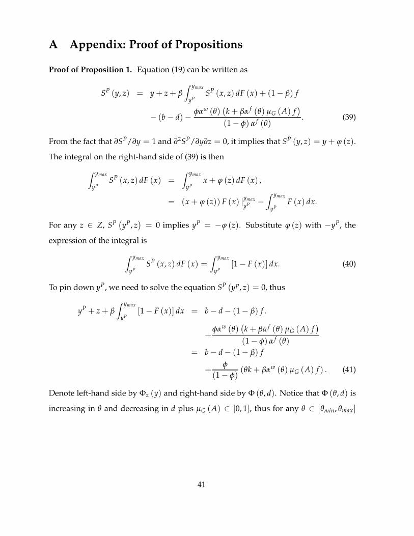
A Appendix: Proof of Propositions

Proof of Proposition 1. Equation (19) can be written as

SP (y, z) = y + z + β∫ ymax

yPSP (x, z) dF (x) + (1− β) f

− (b− d)−φαw (θ)

(

k + βα f (θ) µG (A) f)

(1− φ) α f (θ). (39)

From the fact that ∂SP/∂y = 1 and ∂2SP/∂y∂z = 0, it implies that SP (y, z) = y + ϕ (z).

The integral on the right-hand side of (39) is then

∫ ymax

yPSP (x, z) dF (x) =

∫ ymax

yPx + ϕ (z) dF (x) ,

= (x + ϕ (z)) F (x) |ymax

yP −∫ ymax

yPF (x) dx.

For any z ∈ Z, SP(

yP, z)

= 0 implies yP = −ϕ (z). Substitute ϕ (z) with −yP, the

expression of the integral is

∫ ymax

yPSP (x, z) dF (x) =

∫ ymax

yP[1− F (x)] dx. (40)

To pin down yP, we need to solve the equation SP (yp, z) = 0, thus

yP + z + β∫ ymax

yP[1− F (x)] dx = b− d− (1− β) f .

+φαw (θ)

(

k + βα f (θ) µG (A) f)

(1− φ) α f (θ)

= b− d− (1− β) f

+φ

(1− φ)(θk + βαw (θ) µG (A) f ) . (41)

Denote left-hand side by Φz (y) and right-hand side by Φ (θ, d). Notice that Φ (θ, d) is

increasing in θ and decreasing in d plus µG (A) ∈ [0, 1], thus for any θ ∈ [θmin, θmax]

41

and d ∈ [dmin, dmax],

b− dmax +φ

1− φθmink− (1− β) f < Φ (θ, d)

< b− dmin +φ

1− φ(θmaxk + βαw (θmax) f )− (1− β) f .

Φz (y) is increasing in y and z. If inequalities (22) and (23) holds then for given θ, d and

z, we must have

Φz (ymin) ≤ Φzmax (ymin) < Φ (θ, d) < Φzmin(ymax) ≤ Φz (ymax) .

We can conclude there is a unique solution yP (z) ∈ (ymin, ymax) for equation (41) by

the intermediate value theorem. That is, yP (z) exists for any z ∈ [zmin, zmax].

Similarly, equation (20) can be rewritten as

SR (y, z) = y + z + β∫ ymax

yP[1− F (x)] dx− c− β f − (b− d)

−φαw (θ)

(

k + βα f (θ) µG (A) f)

(1− φ) α f (θ). (42)

Following the same argument for the condition SP(

yP, z)

= 0, the above equation

yields the cut-off value by solving:

yR + z+ β∫ ymax

yP[1− F (x)] dx = b− d+

φαw (θ)(

k + βα f (θ) µG (A) f)

(1− φ) α f (θ)+ c+ β f . (43)

Comparing equations (41) and (43), we get

yR = yP + c + f .

Then assumption 2 guarantees the existence of yP ∈ (ymin, ymax − c− f ) which implies

yR< ymax exists as well.

Proof of Proposition 2. Step 1. Ey JP (y, z) and Ey JT (y, z) are both strictly increasing

in z. From the surplus sharing rule, it is sufficient to show that SP (y, z) and ST (y, z)

42

are strictly increasing in z. Substitute equation (40) into (39), we obtain

SP (y, z) = y + z + β∫ ymax

yP(z)[1− F (x)] dx + (1− β) f − (b− d)

−φαw (θ)

(

k + βα f (θ) µG (A) f)

(1− φ) α f (θ). (44)

Take the derivative of SP with respect to z, we get

∂SP (y, z)

∂z= 1− β

(

1− F(

yP (z)))

yP′ (z) . (45)

From equation (41), the implicit function theorem implies that

yP′ (z) = −1

1− β (1− F (yP))< 0. (46)

Plug (46) into (45), we get ∂SP/∂z > 0. Similarly, the total surplus of a temporary

contract can be rewritten as

ST (y, z) = y + z− b + β (1− αw)∫ ymax

yP(z)+c+ f[1− F (x)] dx. (47)

The derivative of ST with respect to z is given by

∂ST (y, z)

∂z= 1− β (1− αw)

[

1− F(

yP (z))]

yP′ (z) > 0.

Step 2. Ey JP (y, z) and Ey JT (y, z) are strictly convex. By the separability of y and z,

it suffices to prove that SP and STare convex in z. Twice differentiate SP with respect

to z, and get∂2SP (y, z)

∂z2 = β

[

F′(

yP′)2−(

1− F(

yP))

yP′′

]

.

Since yP′′ = βF′yP′/[

1− β(

1− F(

yP))]2

< 0 and F′ > 0, it must be the case that

∂2SP (y, z) /∂z2> 0. Similarly, ∂2ST (y, z) /∂z2

> 0.

These two steps guarantee that if Ey JP (y, z) = Ey JT (y, z) holds, the cut-off value z

43

is unique. The last step is to verify the single crossing property. That is, if

Ey JP (y, zmin) < Ey JT (y, zmin) ,

Ey JP (y, zmax) > Ey JT (y, zmax)

hold, then the cut-off value z exists. Denote

∆θ,d (z) =Ey JP (y, z)− Ey JT (y, z)

1− φ

= β∫ ymax

yP[1− F (x)] dx− β (1− αw (θ))

∫ ymax

yR[1− F (x)] dx + d

−

[

11− φ

− (1− β)

]

f −φ

(1− φ)(θk + βαw (θ) µG (A) f ) .

= b−1

1− φf − yP − z + (E (y) + z) d

−β (1− αw (θ))∫ ymax

yR(z)[1− F (x)] dx.

The last equality is derived by replacing β∫ ymax

yP [1− F (x)] dx with equation (41). No-

tice that equation (41) defines an implicit function yP (z, θ, µG, d). Totally differentiating

(41) yields

∂yP

∂θ=

φ (k + βµG f αw′ (θ))

(1− φ) [1− β (1− F (yP))]> 0,

∂yP

∂µG=

φβ f αw (θ)

(1− φ) [1− β (1− F (yP))]> 0,

∂yP

∂d=

−1[1− β (1− F (yP))]

< 0.

Then

∆θ,d (zmin) ≤ b−1

1− φf − yP (zmin, θmin, 0, d)− zmin, (48)

and

∆θ,d (zmax) ≥ b−1

1− φf − yP (zmax , θmax, 1, d)− zmax (49)

−β (1− αw (θmin))∫ ymax

ymin

[1− F (x)] dx.

44

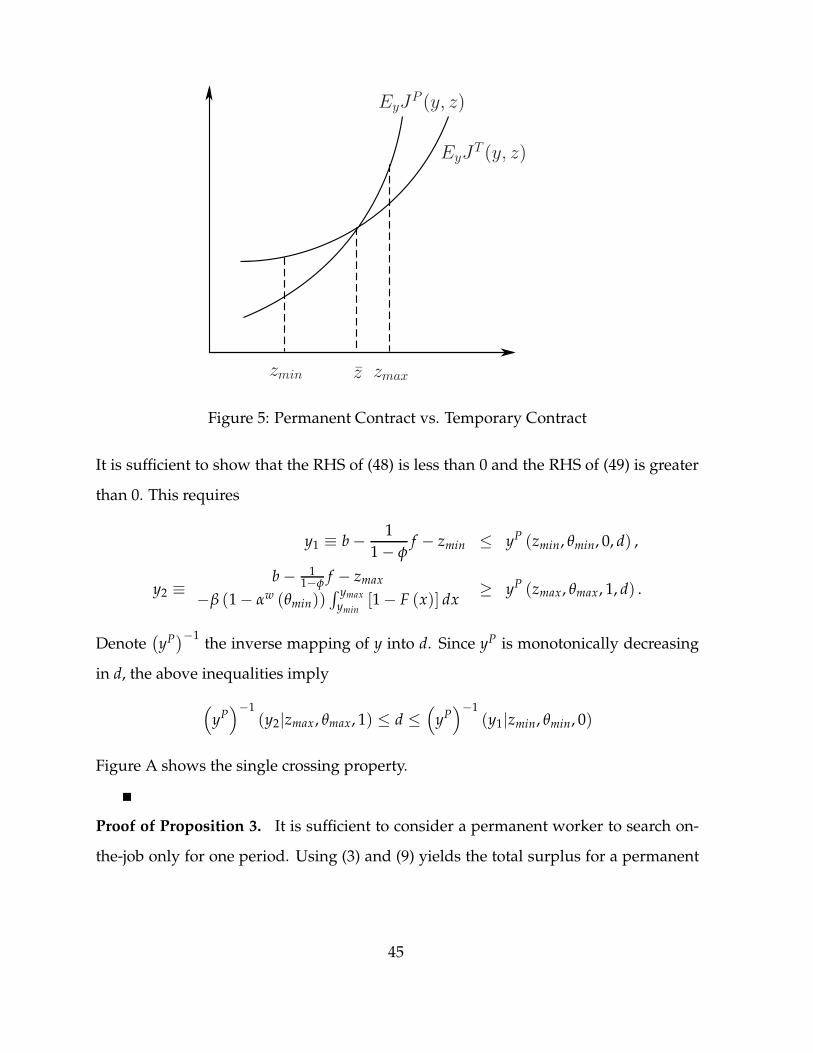
zmin z zmax

EyJP (y, z)

EyJT (y, z)

Figure 5: Permanent Contract vs. Temporary Contract

It is sufficient to show that the RHS of (48) is less than 0 and the RHS of (49) is greater

than 0. This requires

y1 ≡ b−1

1− φf − zmin ≤ yP (zmin, θmin, 0, d) ,

y2 ≡b− 1

1−φ f − zmax

−β (1− αw (θmin))∫ ymax

ymin[1− F (x)] dx

≥ yP (zmax, θmax, 1, d) .

Denote(

yP)−1 the inverse mapping of y into d. Since yP is monotonically decreasing

in d, the above inequalities imply

(

yP)−1

(y2|zmax , θmax, 1) ≤ d ≤(

yP)−1

(y1|zmin, θmin, 0)

Figure A shows the single crossing property.

Proof of Proposition 3. It is sufficient to consider a permanent worker to search on-

the-job only for one period. Using (3) and (9) yields the total surplus for a permanent

45

match of:

SPs (y, z) = JP

s (y, z)− (Q− f ) + VPs (y, z)−U

= y + z + [1− (1− αw (θ))] β f − (b− d) (50)

+β(1− αw(θ)∫ ymax

ymin

max(

SP (y, z) , 0)

dF (x)

If the permanent worker does not search, the total surplus SP (y, z) is given by equation

(19). What we need to show is

SP(y, z) ≥ SPs (y, z)

for any y and z ≥ z. Using (19), (50) and the fact (40), the above inequality holds if and

only if

d ≥φ

1− φ(θk + βαw (θ) µG (A) f )− βαw (θ)

(

∫ ymax

yP[1− F (x)] dx− f

)

. (51)

Denote the right hand side of (51) by Λ.

Λ ≤φ

1− φ(θmaxk + βαw (θmax) f )− βαw (θmin)

(

∫ ymax

yP(zmin,θmax,1,dmin)[1− F (x)] dx− f

)

.

Because d ≥ dmin, if

dmin = max

0,φ

1−φ (θmaxk + βαw (θmax) f )

−βαw (θmin)(

∫ ymax

yP(zmin,θmax,1,dmin)[1− F (x)] dx− f

)

≡ d3

inequality (51) holds. Similar argument can show that the newly promoted worker

will have no incentive to search.

We now show that temporary workers have an incentive to search on the job. Sup-

pose temporary workers do not search for one period. Using (5) and (14) generates the

46

surplus as:

STn = y + z + β

∫ ymax

ymin

max(

SR (x, z) , 0)

dF (x)

− (b− d)−φ

1− φθ(

k + βα f (θ) µG (A) f)

(52)

If temporary workers do search then the surplus is defined by equation (21). Then

ST(y, z) ≥ STn (y, z) requires

d ≤φ

1− φ(θk + βαw (θ) µG (A) f )− βαw(θ)

∫ ymax

yR[1− F(x)]dx. (53)

The right hand side of (51) denoted by Λ must not less than

φ

1− φθmink− βαw(θmax)

∫ ymax

yR(zmax,θmin,0,dmax)[1− F(x)]dx. (54)

Then for any d ≤ dmax, if

dmax =φ

1− φθmink− βαw(θmax)

∫ ymax

yR(zmax,θmin,0,dmax)[1− F(x)]dx

≡ d4

temporary workers have an incentive to search on the job.

Combine conditions in Proposition 2, we have dmin = max (d1, d3) and dmax ≡

min (d2, d4).

Proof of Proposition 4. The equilibrium condition for z is Ey JP (y, z) = Ey JT (y, z). By

using the sharing rule (16) and equations (19) and (21), it implies that

β∫ ymax

yP(1− F (x)) dx−

[

11− φ

− (1− β)

]

f −φ (θk + βαw (θ) (1− G (z)) f )

(1− φ)

+ d− β (1− αw)∫ ymax

yR(1− F (x)) dx = 0 (55)

47

where yP ≡ yP (z) and yR ≡ yR (z) = yP + c + f . From equation (25), we have

yP + z + β∫ ymax

yP(1− F (x)) dx + (1− β) f

− (b− d)−φ (θk + βαw (θ) (1− G (z)) f )

(1− φ)= 0. (56)

Denote the left hand sides of equations (55) and (56) by Π(

yP, z)

. Totally differentiate

Π, we get

D(yP,z)Π =

[

1− β(

1− F(

yP))

1 + φ1−φ αwβ f G′ (z)

−β[

1− F(

yP)

− (1− αw)(

1− F(

yR))] φ

1−φ αwβ f G′ (z)

]

,

and

D f Π =

1− β− φ1−φ αwβ (1− G (z))

−[

11−φ − (1− β)

]

+ β (1− αw)(

1− F(

yR))

−φ

1−φ αwβ (1− G (z))

,

DαwΠ =

− φ

(1−φ)α f

[

k + βα f (1− G (z)) f]

∫ ymax

yR (1− F (x)) dx− φ

(1−φ)α f

[

k + βα f (1− G (z)) f]

,

DcΠ =

[

0β (1− αw)

(

1− F(

yR))

]

.

The determinant of matrix D(yP,z)Π is

∣

∣

∣D(yP,z)Π

∣

∣

∣= β

[

1− F(

yP)

− (1− αw)(

1− F(

yR))]

+[

1− β (1− αw)(

1− F(

yR))]

[

φ

1− φαwβ f G′ (z)

]

> 0,

since F(

yP)

< F(

yR)

and G′ (z) > 0. Apply the implicit function theorem, we can

calculate the following:dz

d f= −

a1 + a2∣

∣

∣D(yP,z)Π

∣

∣

∣

,

where

a1 = β[

1− F(

yP)

− (1− αw)(

1− F(

yR))]

(

1− β−φ

1− φαwβ (1− G (z))

)

48

and

a2 =[

1− β(

1− F(

yP))]

{

−

[

11− φ

− (1− β)

]

+β (1− αw)(

1− F(

yR))

+φ

1− φαwβ (1− G (z))

}

.

Observe that the numerator (a1 + a2) is decreasing in φ. When φ = 0, the numerator

becomes

a1 + a2 = β (1− β)[

1− F(

yP)

− (1− αw)(

1− F(

yR))]

−β[

1− β(

1− F(

yP))] [

1− (1− αw)(

1− F(

yR))]

.

Because 1 − β < 1 − β(

1− F(

yP))

and 1 − F(

yP)

− (1− αw)(

1− F(

yR))

< 1 −

(1− αw)(

1− F(

yR))

, we must have a1 + a2 < 0. Hence, for any φ, dz/d f > 0.

dz

dαw= −

a3∣

∣

∣D(yP,z)Π

∣

∣

∣

,

where

a3 = β[

1− F(

yP)

− (1− αw)(

1− F(

yR))]

{

−φ

(1− φ) α f

[

k + βα f (1− G (z)) f]

}

+[

1− β(

1− F(

yP))]

{

∫ ymax

yR(1− F (x)) dx

−φ

(1− φ) α f

[

k + βα f (1− G (z)) f]

}

.

Again, a3 is decreasing in φ. When φ→ 0, a3 →[

1− β(

1− F(

yP))] ∫ ymax

yR (1− F (x)) dx >

0, while φ→ 1, a3 → −∞. Therefore there exists φ such that{

dzdαw < 0 when φ < φdz

dαw > 0 when φ > φ

dz

dc= −

[

1− β(

1− F(

yP))]

β (1− αw)(

1− F(

yR))

∣

∣

∣D(yP,z)Π

∣

∣

∣

< 0.

49

Proof of Proposition 5. Suppose φ→ 0, equation (41) implies

dyP

d f= −

1− β−φ

1−φ αwβ (1− G (z)) +φ

1−φ αwβ f G′ (z) dzd f

1− β (1− F (yP))

< 0,

dyP

dαw= −

−φ

(1−φ)α f

[

k + βα f (1− G (z)) f]

+φ

1−φ αwβ f G′ (z) dzdαw

1− β (1− F (yP))

> 0,

dyP

dc= −

φ1−φ αwβ f G′ (z) dz

dc

1− β (1− F (yP))→ 0+.

Use these facts and combine equation (43), we derive

dyR

d f=

βF(

yP)

− φ1−φ αwβ

[

(1− G (z))− f G′ (z) dzd f

]

1− β (1− F (yP))> 0,

dyR

dαw=

dyP

dαw> 0,

dyR

d f= 1 +

φ1−φ αwβ f G′ (z) dz

dc

1− β (1− F (yP))> 0.

Proof of Proposition 6. The job creation rule is obtained by equation (17). Substitute

equations (19) and (21) into (17), we get

E (y + z)− b (1− d)−∫ z

zmin

d (E (y) + z) dG (z) + (1− β) (1− G (z)) f

−β + φαw (θ) (1− G (z))

(1− φ) βα f (θ)

[

k + β f (1− G (z)) α f (θ)]

+ β (1− αw (θ))∫ z

zmin

∫ ymax

yP(z)+c+ f(1− F (x)) dxdz

+ β∫ zmax

z

∫ ymax

yP(z)(1− F (x)) dxdz = 0 (57)

Denote the left hand side of equation (57) by h and differentiate it with respect to θ, f

50

and c, one gets:

∂h

∂θ= −βαw′

∫ z

zmin

∫ ymax

yP(z)+c+ f(1− F (x)) dxdz

−k[

φ (1− G (z)) α f αw′ − [β + φαw (θ) (1− G (z))] α f ′]

(1− φ) β(

α f)2

−β + φαw (1− G (z))

(1− φ)(1− G (z)) αw′

< 0,

due to αw′ (θ) > 0 and α f ′ (θ) < 0,

∂h

∂ f= (1− β) (1− G (z))−

β + φαw (1− G (z))

(1− φ)(1− G (z))

−β (1− αw)∫ z

zmin

(

1− F(

yR (z)))

dz.

∂h/∂ f is negative provided that β > 1/2. Hence

dθ

d f= −

∂h/∂ f

∂h/∂θ< 0.

Finally, since∂h

∂c= −β (1− αw)

∫ z

zmin

(

1− F(

yR (z)))

dz < 0,

we can conclude thatdθ

dc= −

∂h/∂c

∂h/∂θ< 0.

51

B Model Solution and Estimation

This section describes some technical aspects of the solution and estimation algorithmsthat produce the results shown in section 7. The model described can be defined as afunction Ξ : Γ → Y, where γ ∈ Γ ⊂ R

nγ , and y ∈ Y ⊂ RnM. An element in the set

Y can be thought of an endogenous variable (e.g. the unemployment rate) that is anoutcome of the model. The estimation procedure uses a statistical criterion functionthat minimizes the deviations of model-implied moments - weighted appropriately -from empirical moments.

Empirical moments are given by the means of time series that have a model-impliedmoment as a counterpart. Given a vector of time series of length T denoted by YT ={

Y1T, . . . , YnM

T

}

define the vector MnM×1 as having typical element mj = (y(γ) − YjT)

with j = 1, . . . , nM and YjT = (1/T)∑

Tt=1 yt. We construct the statistical criterion func-

tion,

H(γ, YT) = M(γ, YT)′W(γ, YT)M(γ, YT) (58)

We sensibly choose the matrix W(γ, YT) to be the inverse of the variance matrix ofYT. In our application nM = 13 and nγ = 8, since the parameter vector of interest isgiven by γ = ( f , b, φ, ξ, k, µy , µz, σy). In principle one can obtain an estimate of γ by:

γ = argminγ

H(γ, YT).

Minimizing the function H(γ, YT) by means of standard minimization routines e.g.any optimizer in the family of Newton-type methods, is seldom an easy task. Prob-lems abound, and they include non-differentiabilities, flat areas, and local minima. Toobtain estimates of γ we employ a Markov Chain Monte Carlo method (MCMC) thattransforms the function H(γ, YT) into a proper density function. This transformationis given by:

p(γ, YT) =eH(γ,YT)

∫

ΓeH(γ,YT)dγ

(59)

where π(γ) is a prior distribution (or weight function) over the parameter space. Thisdistribution can be uniform which implies a constant π(γ) and we assume so in theestimation. Chernozhukov and Hong (2003) label p(γ, YT) a quasi-posterior densitybecause it is not a posterior density function in a true Bayesian sense; there is no up-dating. It is, however, a proper density function with well-defined moments and as aresult we can define, for instance, the quasi-posterior mean as:

γ =∫

Γγp(γ, YT)dγ (60)

In practice, the way we compute the quasi-posterior mean is by a Monte Carlo

52

procedure. Markov Chain Monte Carlo amounts to simulating a Markov Chain thatconverges to the quasi-posterior distribution. Beginning with an initial guess for theparameter vector γ0, we iterate on the following algorithm:

1. Draw a candidate vector γi from a distribution q(γi|γi−1).

2. Compute eH(γi,YT).

3. If pA = eH(γi,YT)

eH(γi−1,YT)≥ 1, accept γi.

4. Else, accept γi with probability pA.

5. Set i ← i + 1 and return to Step 1.

Repeating these 5 steps and generating a long sequence of draws for γ yields asample of large size, hopefully drawn from the quasi posterior density p(γ, YT).25

Any moment of interest (means, standard deviations, quantiles, etc. . . ) can be read-ily computed. To evaluate the function eH(γ, YT) one needs to solve for the modelcounterparts of the empirical series in YT. For a given γi in the sequence of simulateddraws, we obtain a model solution using the following steps:

1. We begin with guesses for θ, and z.26

2. Find the surplus functions SP, SR and ST by substituting and combining equa-tions (19), (20), (21), (42), (44), and (47).

3. Update θ using equation (17). Using the functional form for the matching func-tion specified above, θ is given by:

θ =

(

(

Φ

k

)ξ

− 1

)1ξ

and

Φ =∫ zmax

zmin

[

IAEySP (y, z) + (1− IA)EyST (y, z)]

dG (z) (1− φ)β

−β f µG(A).

There are two important things to consider in this step. First, the initial guess of θis important. Not all values of θ converge. Second, due to the degree of nonlinear-ity in our problem, we dampen the speed of updating θ by heavily weighting theprevious value. We set the updated value θNEW to be equal to λθOLD + (1− λ)θwhere λ is 0.9 (updating is slow).

25We used 5,000 simulations and discarded the first 1,000.26We hope it is clear to the reader the implicit dependence of these variables on γi.

53

4. Update z by solving the two-equation system defined by equations (55) and (56),which solve for z and yP(z).

5. Iterate on the previous two steps until the sequences of θ and z have converged.

6. Having obtained z and θ we can update the employment measures - both tempo-rary and permanent - using the steady-state versions of equations (32) and (33).These are given by:

nP =

(

u + nT)

αw (θ) (1− G (z))

1−∫ zmax

zmin[1− F (yP (z))] dG (z)

+(1− αw (θ))

∫ zzmin

[

1− F(

yR (z))]

dG (z) nT

1−∫ zmax

zmin[1− F (yP (z))] dG (z)

.

and,

nT =uαw (θ) G (z)

1− αw (θ) G (z).

All integrals throughout are evaluated using quadrature. With values for θ, z, nT ,nP (and clearly u as a byproduct), one can compute wages and simulate histories ofworkers to fit regression equation (37). In addition, it is easy to compute other mo-ments. In what follows we summarize how we compute the measures of turnover forthe different groups of workers.

• Job destruction rate for all workers:

JD =∫ zmax

zmin

F(YP(z))dG(z)nP

nP + nT+ (1− αw)

1G(z)

∫ z

zmin

F(YR(z))dG(z)nT

nP + nT

• Job creation rate for all workers:

JC =u

nT + nPαw

• Job destruction rate for permanent workers:

JDP =∫ zmax

zmin

F(YP(z))dG(z)nP

nP + nT

• Job creation rate for permanent workers:

JCP = αw(1− G(z))nT + u

nP + nT+ (1− αw)

∫ z

zmin

(1− F(YR(z)))dG(z)nT

nP + nT

54

• Job destruction rate for temporary workers:

JDT = (1− αw)nT

nT + nP+ αw(1− G(z))

nT

nP + nT

• Job destruction rate for temporary workers:

JCT = αwG(z)u

nP + nT

55