Math. Program., Ser. ADOI 10.1007/s10107-012-0583-2

FULL LENGTH PAPER

Fixed-charge transportation on a path: optimization,LP formulations and separation

Mathieu Van Vyve

Received: 16 May 2011 / Accepted: 12 July 2012© Springer and Mathematical Optimization Society 2012

Abstract In the fixed-charge transportation problem, the goal is to optimallytransport goods from depots to clients when there is a fixed cost associated to trans-portation or, equivalently, to opening an arc in the underlying bipartite graph. Wefurther motivate its study by showing that it is both a special case and a strong relax-ation of the big-bucket multi-item lot-sizing problem, and a generalization of a simplevariant of the single-node flow set. This paper is essentially a polyhedral analysis ofthe polynomially solvable special case in which the associated bipartite graph is a path.We give a O(n3)-time optimization algorithm and a O(n2)-size linear programmingextended formulation. We describe a new class of inequalities that we call “path-modular” inequalities. We give two distinct proofs of their validity. The first one isdirect and crucially relies on sub- and super-modularity of an associated set function.The second proof is by showing that the projection of the extended linear programmingformulations onto the original variable space yields exactly the polyhedron describedby the path-modular inequalities. Thus we also show that these inequalities suffice todescribe the convex hull of the set of feasible solutions.

Keywords Mixed-integer programming · Lot-sizing · Transportation ·Convex hull · Extended formulation

Mathematics Subject Classification (2000) 68Q25 · 90C11 · 90C27 · 90C35 ·90B05 · 90B06

This text presents research results of the Belgian Program on Interuniversity Poles of Attraction initiatedby the Belgian State, Prime Minister’s Office, Science Policy Programming. The scientific responsibilityis assumed by the author.

M. Van Vyve (B)CORE, voie du Roman Pays 34 bte L1.03.01, 1348 Louvain-la-Neuve, Belgiume-mail: mathieu.vanvyve@uclouvain.be

123

M. Van Vyve

1 Introduction

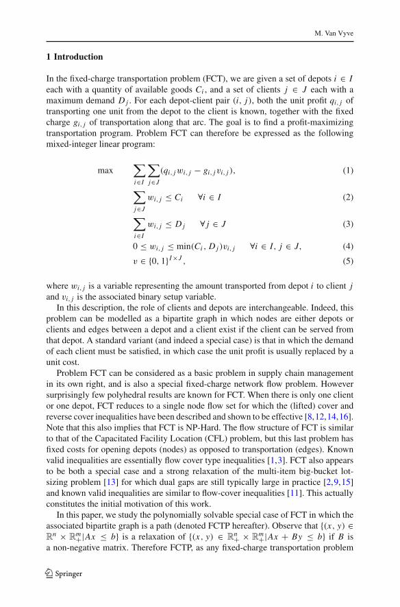
In the fixed-charge transportation problem (FCT), we are given a set of depots i ∈ Ieach with a quantity of available goods Ci , and a set of clients j ∈ J each with amaximum demand D j . For each depot-client pair (i, j), both the unit profit qi, j oftransporting one unit from the depot to the client is known, together with the fixedcharge gi, j of transportation along that arc. The goal is to find a profit-maximizingtransportation program. Problem FCT can therefore be expressed as the followingmixed-integer linear program:

max∑

i∈I

∑

j∈J

(qi, jwi, j − gi, jvi, j ), (1)

∑

j∈J

wi, j ≤ Ci ∀i ∈ I (2)

∑

i∈I

wi, j ≤ D j ∀ j ∈ J (3)

0 ≤ wi, j ≤ min(Ci , D j )vi, j ∀i ∈ I, j ∈ J, (4)

v ∈ {0, 1}I×J , (5)

where wi, j is a variable representing the amount transported from depot i to client jand vi, j is the associated binary setup variable.

In this description, the role of clients and depots are interchangeable. Indeed, thisproblem can be modelled as a bipartite graph in which nodes are either depots orclients and edges between a depot and a client exist if the client can be served fromthat depot. A standard variant (and indeed a special case) is that in which the demandof each client must be satisfied, in which case the unit profit is usually replaced by aunit cost.

Problem FCT can be considered as a basic problem in supply chain managementin its own right, and is also a special fixed-charge network flow problem. Howeversurprisingly few polyhedral results are known for FCT. When there is only one clientor one depot, FCT reduces to a single node flow set for which the (lifted) cover andreverse cover inequalities have been described and shown to be effective [8,12,14,16].Note that this also implies that FCT is NP-Hard. The flow structure of FCT is similarto that of the Capacitated Facility Location (CFL) problem, but this last problem hasfixed costs for opening depots (nodes) as opposed to transportation (edges). Knownvalid inequalities are essentially flow cover type inequalities [1,3]. FCT also appearsto be both a special case and a strong relaxation of the multi-item big-bucket lot-sizing problem [13] for which dual gaps are still typically large in practice [2,9,15]and known valid inequalities are similar to flow-cover inequalities [11]. This actuallyconstitutes the initial motivation of this work.

In this paper, we study the polynomially solvable special case of FCT in which theassociated bipartite graph is a path (denoted FCTP hereafter). Observe that {(x, y) ∈R

n × Rm+|Ax ≤ b} is a relaxation of {(x, y) ∈ R

n+ × Rm+|Ax + By ≤ b} if B is

a non-negative matrix. Therefore FCTP, as any fixed-charge transportation problem

123

Fixed-charge transportation on a path: LP formulations

defined on a class of subgraphs of the complete bipartite graph, is a relaxation of FCT.It can therefore be hoped that polyhedral results for FCTP will be helpful in solvingthe more general FCT, or give theoretical insight for deriving strong inequalities forFCT.

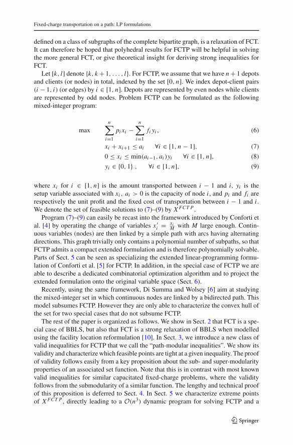
Let [k, l] denote {k, k+ 1, . . . , l}. For FCTP, we assume that we have n+ 1 depotsand clients (or nodes) in total, indexed by the set [0, n]. We index depot-client pairs(i − 1, i) (or edges) by i ∈ [1, n]. Depots are represented by even nodes while clientsare represented by odd nodes. Problem FCTP can be formulated as the followingmixed-integer program:

maxn∑

i=1

pi xi −n∑

i=1

fi yi , (6)

xi + xi+1 ≤ ai ∀i ∈ [1, n − 1], (7)

0 ≤ xi ≤ min(ai−1, ai )yi ∀i ∈ [1, n], (8)

yi ∈ {0, 1} , ∀i ∈ [1, n], (9)

where xi for i ∈ [1, n] is the amount transported between i − 1 and i, yi is thesetup variable associated with xi , ai > 0 is the capacity of node i , and pi and fi arerespectively the unit profit and the fixed cost of transportation between i − 1 and i .We denote the set of feasible solutions to (7)–(9) by X FCT P .

Program (7)–(9) can easily be recast into the framework introduced by Conforti etal. [4] by operating the change of variables x ′i = xi

M with M large enough. Contin-uous variables (nodes) are then linked by a simple path with arcs having alternatingdirections. This graph trivially only contains a polynomial number of subpaths, so thatFCTP admits a compact extended formulation and is therefore polynomially solvable.Parts of Sect. 5 can be seen as specializing the extended linear-programming formu-lation of Conforti et al. [5] for FCTP. In addition, in the special case of FCTP we areable to describe a dedicated combinatorial optimization algorithm and to project theextended formulation onto the original variable space (Sect. 6).

Recently, using the same framework, Di Summa and Wolsey [6] aim at studyingthe mixed-integer set in which continuous nodes are linked by a bidirected path. Thismodel subsumes FCTP. However they are only able to characterize the convex hull ofthe set for two special cases that do not subsume FCTP.

The rest of the paper is organized as follows. We show in Sect. 2 that FCT is a spe-cial case of BBLS, but also that FCT is a strong relaxation of BBLS when modelledusing the facility location reformulation [10]. In Sect. 3, we introduce a new class ofvalid inequalities for FCTP that we call the “path-modular inequalities”. We show itsvalidity and characterize which feasible points are tight at a given inequality. The proofof validity follows easily from a key proposition about the sub- and super-modularityproperties of an associated set function. Note that this is in contrast with most knownvalid inequalities for similar capacitated fixed-charge problems, where the validityfollows from the submodularity of a similar function. The lengthy and technical proofof this proposition is deferred to Sect. 4. In Sect. 5 we characterize extreme pointsof X FCT P , directly leading to a O(n3) dynamic program for solving FCTP and a

123

M. Van Vyve

linear-programming extended formulations with O(n2) nonnegative variables, O(n2)

inequality constraints and O(n2) non-zero coefficients. We characterize its projectiononto the original variable space in Sect. 6. We show that the inequalities we obtainare precisely the path-modular inequalities, thereby showing that they are sufficient todescribe the convex hull of X FCT P . Section 7 shows that the path-modular inequali-ties introduced in this paper can explain some facets of the fixed-charge transportationproblem on complete bipartite graph (FCT). We conclude by discussing future researchon the topic.

Notation. Throughout this paper we use the following notation: [k, l] = {k, k +1, . . . , l}, N = [1, n], E and O denote the even and odd integers respectively, eidenotes the unit vector with component i equal to 1 and all others components equalto 0 and 1 denotes the all-ones vector.

2 Fixed-charge transportation and big-bucket multi-item lot-sizing

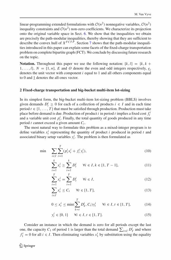
In its simplest form, the big-bucket multi-item lot-sizing problem (BBLS) involvesgiven demands Di

t ≥ 0 for each of a collection of products i ∈ I and in each timeperiod t ∈ {1, . . . , T } that must be satisfied through production. Production must takeplace before demand is due. Production of product i in period t implies a fixed cost f i

tand a variable unit cost pi

t . Finally, the total quantity of goods produced in any timeperiod t cannot exceed a given amount Ct .

The most natural way to formulate this problem as a mixed-integer program is todefine variables xi

t representing the quantity of product i produced in period t andassociated binary setup variables yi

t . The problem is then formulated as

min∑

i∈I

T∑

t=1

(pit xi

t + f it yi

t ), (10)

k∑

t=1

xit ≥

k∑

t=1

Dit ∀i ∈ I, k ∈ [1, T − 1], (11)

T∑

t=1

xit =

T∑

t=1

Dit ∀i ∈ I, (12)

∑

i∈I

xit ≤ Ct ∀t ∈ [1, T ], (13)

0 ≤ xit ≤ min(

T∑

k=t

Dik, Ct )yi

t ∀i ∈ I, t ∈ [1, T ], (14)

yit ∈ {0, 1} ∀i ∈ I, t ∈ [1, T ]. (15)

Consider an instance in which the demand is zero for all periods except the lastone, the capacity C1 of period 1 is larger than the total demand

∑i∈I Di

T and wheref i1 = 0 for all i ∈ I . Then eliminating variables xi

1 by substitution using the equality

123

Fixed-charge transportation on a path: LP formulations

constraints (12), we obtain:

min∑

i∈I

T∑

t=2

((pit − pi

1)xit + f i

t yit )+ constant,

T∑

t=2

xit ≤ Di

T ∀i ∈ I,

∑

i∈I

xit ≤ Ct ∀t ∈ [2, T ],

0 ≤ xit ≤ min(Di

T , Ct )yit ∀i ∈ I, t ∈ [2, T ],

yit ∈ {0, 1} ∀i ∈ I, t ∈ [2, T ].

This last problem is exactly a fixed-charge transportation problem with set of depots{2, . . . , T } and set of clients I . Therefore FCT is a special case of BBLS and one haslittle hope to solve BBLS efficiently if one cannot solve FCT efficiently.

Furthermore, we now show that, besides being a special case of BBLS, FCT is also astrong relaxation of BBLS. Improving the formulation (11)–(15), the stronger facilitylocation reformulation [10] of BBLS is obtained by defining variables zi

t,k representingthe quantity of product i produced in period t to satisfy demand in period k:

min∑

i∈I

T∑

t=1

(T∑

k=t

pit zi

t,k + f it yi

t

), (16)

k∑

t=1

zit,k = Di

k ∀i ∈ I, k ∈ [1, T ], (17)

∑

i∈I

T∑

k=t

zit,k ≤ Ct ∀t ∈ [1, T ], (18)

0 ≤ zit,k ≤ min(Ct , Di

k)yit ∀i ∈ I, k, t ∈ [1, T ], (19)

yit ∈ {0, 1} ∀i ∈ I, t ∈ [1, T ]. (20)

Firstly, because∑

i∈I∑T

t=1∑T

k=t zit,k sums to the constant

∑i∈I

∑Tk=1 Di

k byconstraints (17), we can replace the equality constraint (17) by a ≤ constraint if wereplace pi

t by pit −M in the objective (with M large enough). This will not modify the

set of optimal solutions. Secondly, we replace variables yit by variables yi

t,k together

with constraints yit,k = yi

t,k+1 for all k < T .

min∑

i∈I

T∑

t=1

(T∑

k=t

((pit − M)zi

t,k + f it yi

t,T

), (21)

k∑

t=1

zit,k ≤ Di

k ∀i ∈ I, k ∈ [1, T ], (22)

123

M. Van Vyve

∑

i∈I

T∑

k=t

zit,k ≤ Ct ∀t ∈ [1, T ], (23)

0 ≤ zit,k ≤ min(Ct , Di

k)yit,k ∀i ∈ I, k, t ∈ [1, T ], (24)

yit,k ∈ {0, 1} ∀i ∈ I, t ∈ [1, T ], (25)

yit,k−1 = yi

t,k ∀i ∈ I, t ∈ [1, T ], k ∈ [2, T ], (26)

Relaxing the last constraint, we obtain exactly a fixed-charge transportation problemwith depots {1, . . . , T } and clients I ×{1, . . . , T } in which depot t cannot serve client(i, k) if t > k (i.e. the bipartite graph is not complete unless backlogging was allowed).This shows that BBLS is equivalent to FCT, but with setup costs on families of arcs(instead of individual arcs) having the same variable cost.

These tight links between BBLS and FCT motivate the hope that a better under-standing of the polyhedral structure of the convex hull of solutions to FCT may helpin solving BBLS more efficiently.

3 Path-modular inequalities

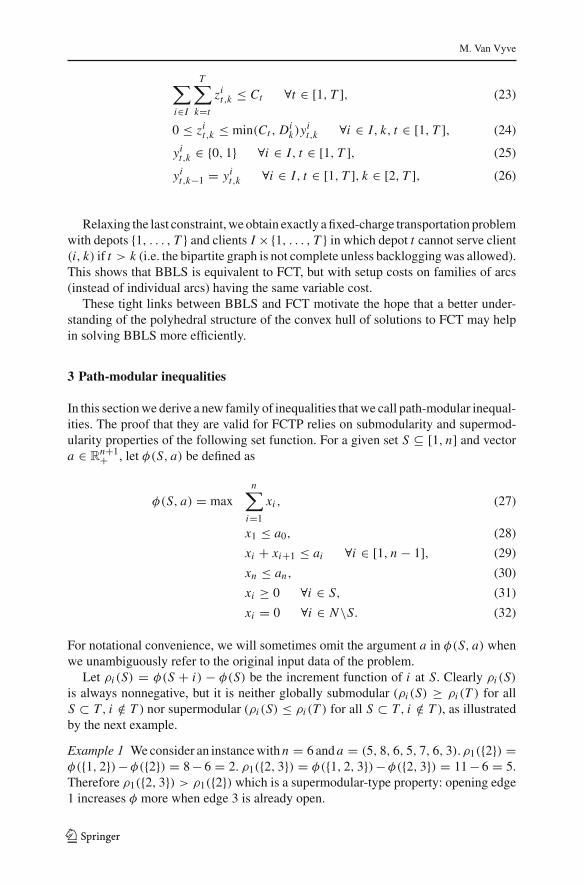
In this section we derive a new family of inequalities that we call path-modular inequal-ities. The proof that they are valid for FCTP relies on submodularity and supermod-ularity properties of the following set function. For a given set S ⊆ [1, n] and vectora ∈ R

n+1+ , let φ(S, a) be defined as

φ(S, a) = maxn∑

i=1

xi , (27)

x1 ≤ a0, (28)

xi + xi+1 ≤ ai ∀i ∈ [1, n − 1], (29)

xn ≤ an, (30)

xi ≥ 0 ∀i ∈ S, (31)

xi = 0 ∀i ∈ N\S. (32)

For notational convenience, we will sometimes omit the argument a in φ(S, a) whenwe unambiguously refer to the original input data of the problem.

Let ρi (S) = φ(S + i) − φ(S) be the increment function of i at S. Clearly ρi (S)

is always nonnegative, but it is neither globally submodular (ρi (S) ≥ ρi (T ) for allS ⊂ T, i /∈ T ) nor supermodular (ρi (S) ≤ ρi (T ) for all S ⊂ T, i /∈ T ), as illustratedby the next example.

Example 1 We consider an instance with n = 6 and a = (5, 8, 6, 5, 7, 6, 3). ρ1({2}) =φ({1, 2})−φ({2}) = 8− 6 = 2. ρ1({2, 3}) = φ({1, 2, 3})−φ({2, 3}) = 11− 6 = 5.Therefore ρ1({2, 3}) > ρ1({2}) which is a supermodular-type property: opening edge1 increases φ more when edge 3 is already open.

123

Fixed-charge transportation on a path: LP formulations

But ρ1(∅) = φ({1}) − φ(∅) = 5 − 0 = 5. Therefore ρ1({2}) < ρ1(∅) which issubmodular-like.

However, as the next proposition shows, we are still able to characterize the sub-and super-modularity of φ. In a nutshell, it tells us that φ exhibits supermodularitywhen we keep on opening edges of the same parity as the edge i under consideration.Conversely, it tells us also that φ exhibits submodularity when we keep on openingedges of the opposite parity compared to the edge i under consideration. Note that,broadly speaking, this is also the case for the single-node flow set and associated flowcover inequalities: in that case each edge is at an odd distance from any other one, sothat the associated max-flow function is completely submodular.

Proposition 1 Let S ⊂ T ⊆ N and i ∈ N\T be given.

(i) If (T \S) ⊆ E and i ∈ E, then ρi (T ) ≥ ρi (S).(ii) If (T \S) ⊆ O and i ∈ O, then ρi (T ) ≥ ρi (S).

(iii) If (T \S) ⊆ E and i ∈ O, then ρi (T ) ≤ ρi (S).(iv) If (T \S) ⊆ O and i ∈ E, then ρi (T ) ≤ ρi (S).

This result is a corollary of a slightly more general theorem. We differ the fairlytechnical proof of these results to the next section to keep the text readable.

We now define the path-modular inequalities. Let L be a subinterval [l, l ′] ofN , let L = OL ∪ EL be the partition of L into odd and even numbers, and letL = ( j1, j2, . . . , j|L|) be a permutation of L . Let O jk

L = { j1, . . . , jk} ∩ OL and

let E jkL = { j1, . . . , jk−1} ∩ EL . We call the following inequality the (l, l ′,L)-path-

modular inequality:

∑

i∈L

xi ≤ φ(OL)+∑

i∈EL

ρi (OL ∪ EiL\Oi

L)yi−∑

i∈OL

ρi (OL ∪ EiL\Oi

L)(1−yi ) (33)

The following proposition characterizes for which values of y (or equivalently whichedges are opened and closed) a given path-modular inequality can be tight. Broadlyspeaking, all path-modular inequalities are tight at points with exactly either all oddor all even edges open. For a fixed subpath L = [l, l ′], the path-modular inequalitiesdiffer in the order in which even edges are opened and odd edges are closed to go fromthe all-odd-edges open to the all-even-edges open situations. The result will also play akey role in showing that the path-modular inequalities are identical to the inequalitiesobtained by projection.

Proposition 2 Let an interval L = [l, l ′] and a permutation L = ( j1, j2, . . . , j|L|)of L be given. For each k ∈ [0, |L|], there exists a point (xk, yk) ∈ X FCT P which istight for the corresponding (l, l ′,L)-path-modular inequality, satisfying

yk =∑

i∈OL

ei +k∑

l=1

e jl (mod 2) (34)

and at which the inequality reduces to∑

i∈N xi ≤ φ(Y k) where Y k = {i ∈ N :yk

i = 1}.

123

M. Van Vyve

Proof We first prove that the right-hand side of the path-modular inequality reducesto φ(Y k) for yk defined according to (34). The proof of this claim is by inductionon k.

For k = 0, Y 0 = OL by definition and the right-hand side of (33) is equal toφ(OL) because y0

i = 0 for i ∈ EL and y0i = 1 for i ∈ OL . Therefore the claim holds.

So let us assume that the claim is true for k − 1 and k > 0. If jk is even, thenY k = Y k−1 + { jk}. Moreover the right-hand side of (33) is equal to φ(Y k−1) +ρ jk (OL ∪ E jk

L \O jkL ) by the induction hypothesis. This last expression is itself equal to

φ(Y k−1)+ ρ jk (Yk−1) = φ(Y k−1 + jk) = φ(Y k). If jk is odd, then Y k = Y k−1\{ jk}.

Moreover the right-hand side of (33) is equal to φ(Y k−1)− ρ jk (OL ∪ E jkL \ O jk

L ) =φ(Y k−1)− ρ jk (Y

k−1 − jk) = φ(Y k−1 − jk) = φ(Y k). Therefore the claim holds.Now, for yk defined according to (34), the inequality reduces to

∑i∈N xi ≤ φ(Y k).

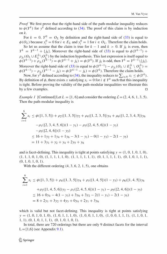
By definition of φ, there exists x satisfying xi = 0 for i /∈ Y k such that this inequalityis tight. Before proving the validity of the path-modular inequalities we illustrate thisby a few examples. � Example 1 [Continued] Let L = [1, 6] and consider the ordering L=(2, 4, 6, 1, 3, 5).Then the path-modular inequality is

6∑

i=1

xi ≤ φ({1, 3, 5})+ ρ2({1, 3, 5})y2 + ρ4({1, 2, 3, 5})y4 + ρ6({1, 2, 3, 4, 5})y6

−ρ1({2, 3, 4, 5, 6})(1− y1)− ρ3({2, 4, 5, 6})(1− y3)

−ρ5({2, 4, 6})(1− y5)

≤ 16+ 1y2 + 1y4 + 1y6 − 3(1− y1)− 0(1− y3)− 2(1− y5)

= 11+ 3y1 + y2 + y4 + 2y5 + y6

and is facet-defining. This inequality is tight at points satisfying y = (1, 0, 1, 0, 1, 0),

(1, 1, 1, 0, 1, 0), (1, 1, 1, 1, 1, 0), (1, 1, 1, 1, 1, 1), (0, 1, 1, 1, 1, 1), (0, 1, 0, 1, 1, 1),

(0, 1, 0, 1, 0, 1).With the different ordering (4, 3, 6, 2, 1, 5), one obtains

6∑

i=1

xi ≤ φ({1, 3, 5})+ ρ4({1, 3, 5})y4 + ρ3({1, 4, 5})(1− y3)+ ρ6({1, 4, 5})y6

+ρ2({1, 4, 5, 6})y2 − ρ1({2, 4, 5, 6})(1− y1)− ρ5({2, 4, 6})(1− y5)

≤ 16+ 0y4 − 4(1− y3)+ 3y6 + 3y2 − 2(1− y1)− 2(1− y5)

= 8+ 2y1 + 3y2 + 4y3 + 0y4 + 2y1 + 3y6

which is valid but not facet-defining. This inequality is tight at points satisfyingy = (1, 0, 1, 0, 1, 0), (1, 0, 1, 1, 1, 0), (1, 0, 0, 1, 1, 0), (1, 0, 0, 1, 1, 1), (1, 1, 0, 1,

1, 1), (0, 1, 0, 1, 1, 1), (0, 1, 0, 1, 0, 1).In total, there are 720 orderings but there are only 9 distinct facets for the interval

L= [1,6] (see Appendix 9.1).

123

Fixed-charge transportation on a path: LP formulations

The proof of the validity of the path-modular inequalities directly follows fromProposition 1.

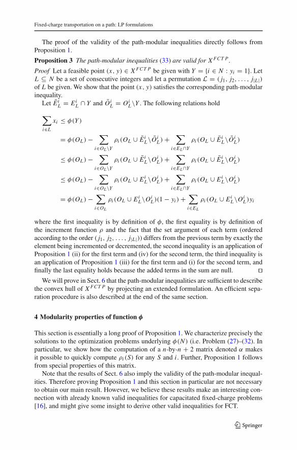
Proposition 3 The path-modular inequalities (33) are valid for X FCT P .

Proof Let a feasible point (x, y) ∈ X FCT P be given with Y = {i ∈ N : yi = 1}. LetL ⊆ N be a set of consecutive integers and let a permutation L = ( j1, j2, . . . , j|L|)of L be given. We show that the point (x, y) satisfies the corresponding path-modularinequality.

Let E iL = Ei

L ∩ Y and OiL = Oi

L\Y . The following relations hold

∑

i∈L

xi ≤ φ(Y )

= φ(OL)−∑

i∈OL\Yρi (OL ∪ E i

L\OiL)+

∑

i∈EL∩Y

ρi (OL ∪ E iL\Oi

L)

≤ φ(OL)−∑

i∈OL\Yρi (OL ∪ E i

L\OiL)+

∑

i∈EL∩Y

ρi (OL ∪ E iL\Oi

L)

≤ φ(OL)−∑

i∈OL\Yρi (OL ∪ Ei

L\OiL)+

∑

i∈EL∩Y

ρi (OL ∪ EiL\Oi

L)

= φ(OL)−∑

i∈OL

ρi (OL ∪ EiL\Oi

L)(1− yi )+∑

i∈EL

ρi (OL ∪ EiL\Oi

L)yi

where the first inequality is by definition of φ, the first equality is by definition ofthe increment function ρ and the fact that the set argument of each term (orderedaccording to the order ( j1, j2, . . . , j|L|)) differs from the previous term by exactly theelement being incremented or decremented, the second inequality is an application ofProposition 1 (ii) for the first term and (iv) for the second term, the third inequality isan application of Proposition 1 (iii) for the first term and (i) for the second term, andfinally the last equality holds because the added terms in the sum are null. �

We will prove in Sect. 6 that the path-modular inequalities are sufficient to describethe convex hull of X FCT P by projecting an extended formulation. An efficient sepa-ration procedure is also described at the end of the same section.

4 Modularity properties of function φ

This section is essentially a long proof of Proposition 1. We characterize precisely thesolutions to the optimization problems underlying φ(N ) (i.e. Problem (27)–(32). Inparticular, we show how the computation of a n-by-n + 2 matrix denoted α makesit possible to quickly compute ρi (S) for any S and i . Further, Proposition 1 followsfrom special properties of this matrix.

Note that the results of Sect. 6 also imply the validity of the path-modular inequal-ities. Therefore proving Proposition 1 and this section in particular are not necessaryto obtain our main result. However, we believe these results make an interesting con-nection with already known valid inequalities for capacitated fixed-charge problems[16], and might give some insight to derive other valid inequalities for FCT.

123

M. Van Vyve

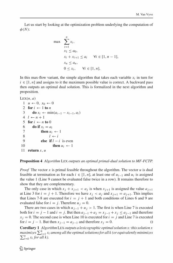
Let us start by looking at the optimization problem underlying the computation ofφ(N ):

maxn∑

i=1

xi ,

x1 ≤ a0,

xi + xi+1 ≤ ai ∀i ∈ [1, n − 1],xn ≤ an,

0 ≤ xi , ∀i ∈ [1, n],In this max-flow variant, the simple algorithm that takes each variable xi in turn fori ∈ [1, n] and assigns to it the maximum possible value is correct. A backward passthen outputs an optimal dual solution. This is formalized in the next algorithm andproposition.

Lex(n, a)

1 u ← 0, x0 ← 02 for i ← 1 to n3 do xi ← min(ai−1 − xi−1, ai )

4 l ← n + 15 for i ← n to 06 do if xi = ai

7 then ui ← 18 l ← i9 else if l − i is even

10 then ui ← 111 return x, u

Proposition 4 Algorithm Lex outputs an optimal primal-dual solution to MF-FCTP.

Proof The vector x is primal feasible throughout the algorithm. The vector u is dualfeasible at termination as for each i ∈ [1, n], at least one of ui−1 and ui is assignedthe value 1 (Line 9 cannot be evaluated false twice in a row). It remains therefore toshow that they are complementary.

The only case in which x j + x j+1 < a j is when x j+1 is assigned the value a j+1at Line 3 for i = j + 1. Therefore we have x j < a j and x j+1 = a j+1. This impliesthat Lines 7-8 are executed for i = j + 1 and both conditions of Lines 6 and 9 areevaluated false for i = j . Therefore u j = 0.

There are two cases in which u j−1 + u j > 1. The first is when Line 7 is executedboth for i = j − 1 and i = j . But then a j−1 + a j = x j−1 + x j ≤ a j−1 and thereforex j = 0. The second case is when Line 10 is executed for i = j and Line 7 is executedfor i = j − 1. But then x j−1 = a j−1 and therefore x j = 0. � Corollary 1 Algorithm Lex outputs a lexicographic optimal solution x: this solution xmaximizes

∑ki=1 xi among all the optimal solutions for all k (or equivalently minimizes∑n

i=k xi for all k).

123

Fixed-charge transportation on a path: LP formulations

Proof For k < n, Lex(k, a) assigns the same values to x1, . . . , xk as Lex(n, a). Itremains to note that by Proposition 4 Lex(k, a) outputs a solution that maximizes∑k

i=1 xi . � Let us define the following set of values for i ∈ [1, n] and j ∈ [0, n + 1] :

αi, j =⎧⎨

⎩

0 if j = i,min(ai−1 − αi−1, j , ai ) if j < i,min(ai − αi+1, j , ai−1) if j > i,

assuming α0,0 = αn+1,n+1 = 0. Lex precisely outputs xi = αi,0. Let Rev- Lex be thesame algorithm as Lex but starting from xn+1 = 0 and working in decreasing order ofi . Rev- Lex yields another optimal solution, but one that is lexicographically reverse.The value for x output by Rev- Lex is αi,n+1.

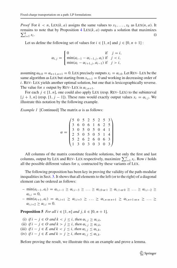
For each j ∈ [1, n], one could also apply Lex (resp. Rev- Lex) to the subinterval[ j + 1, n] (resp. [1, j − 1]). These runs would exactly output values xi = αi, j . Weillustrate this notation by the following example.

Example 1 [Continued] The matrix α is as follows:

α =

⎛

⎜⎜⎜⎜⎜⎜⎝

5 0 5 2 5 2 5 33 6 0 6 1 6 2 53 0 5 0 5 0 4 12 5 0 5 0 5 1 45 2 6 2 6 0 6 31 3 0 3 0 3 0 3

⎞

⎟⎟⎟⎟⎟⎟⎠

All columns of the matrix constitute feasible solutions, but only the first and lastcolumns, output by Lex and Rev- Lex respectively, maximize

∑ni=1 xi . Row i holds

all the possible different values for xi contructed by these variants of Lex.

The following proposition has been key in proving the validity of the path-modularinequalities in Sect. 3. It shows that all elements to the left (or to the right) of a diagonalelement can be ordered as follows:

– min(ai−1, ai ) = αi,i−1 ≥ αi,i−3 ≥ . . . ≥ αi,0 or 1 ≥ αi,1 or 0 ≥ . . . ≥ αi,i−2 ≥αi,i = 0,

– min(ai+1, ai ) = αi,i+1 ≥ αi,i+3 ≥ . . . ≥ αi,n or n+1 ≥ αi,n+1 or n ≥ . . . ≥αi,i+2 ≥ αi,i = 0.

Proposition 5 For all i ∈ [1, n] and j, k ∈ [0, n + 1],(i) if i − j ∈ O and k < j ≤ i , then αi, j ≥ αi,k ,

(ii) if i − j ∈ O and k > j ≥ i , then αi, j ≥ αi,k ,(iii) if i − j ∈ E and k < j ≤ i , then αi, j ≤ αi,k ,(iv) if i − j ∈ E and k > j ≥ i , then αi, j ≤ αi,k .

Before proving the result, we illustrate this on an example and prove a lemma.

123

M. Van Vyve

Example 1 [Continued] On the second row of α, starting from position (2, 3), we walkto the right skipping one element at each step, then walk back to the diagonal elementthrough the skipped elements to obtain (6, 6, 5, 2, 1, 0). This is indeed a decreasingsequence.

Lemma 1 1. αi,0 isa. monotonously increasing with ai ,b. monotonously increasing with ai−t for t odd,c. monotonously decreasing with ai−t for t even,

2. αi,n+1 isa. monotonously increasing with ai−1,b. monotonously increasing with ai+t for t even,c. monotonously decreasing with ai+t for t odd,

Proof We start with trivial observations:

– O1: min(a, b) is increasing with a or b if a does not depend on b and conversely,– O2: a −min(b, a) is increasing in a if b is independent of a.– O3: A decreasing function of an increasing (resp. decreasing) function is decreas-

ing (resp. increasing).

α1,0 = min(a0, a1) is increasing with a0 and a1. α2,0 = min(a1 − α1,0, a2) isincreasing with a2 by O1, increasing with a1 by O2 and decreasing with a0 by O3.α3,0 = min(a2 − α2,0, a3) is increasing with a3 by O1, increasing with a2 by O2,decreasing with a1 by O3 and increasing with a0 by O3.

Iterating this argument yields 1(a), 1(b) and 1(c). Cases 2 are similar to case 1. � Proof of Proposition 5 Case (i). Let the two vectors a j , ak ∈ R

n+1 be defined asfollows:

a jl =

{0 if l = k − 1or l = j − 1,

al otherwiseak

l ={

0 if l = k − 1,

al otherwise

so that ak is obtained from a j by increasing the j − 1th component.

Claim 1 αi, j is the value for xi output by Lex(n, a j ). Indeed, regardless of the valuesassigned to x1, . . . , x j−1, Lex(n, a j ) will set x j = 0 = α j, j , then xi = min(ai−1 −xi−1, ai ) = min(ai−1 − αi−1, j , ai ) = αi, j by induction on i .

Claim 2 αi,k is the value for xi output by Lex(n, ak). Indeed, regardless of the valuesassigned to x1, . . . , xk−1, Lex(n, ak) will set xk = 0 = αk,k , then xi = min(ai−1 −xi−1, ai ) = min(ai−1 − αi−1,k, ai ) = αi,k by induction on i .

Now, Lemma 1 case 1.c applies so that the value for xi output by Lex(n, a j ) islarger than the value for xi output by Lex(n, ak), or equivalently αi, j ≥ αi,k . Theother cases are similar. �

The next lemma characterizes ρi (N − i) or what can be gained in φ by openingarc i when all the other arcs are open. The result then easily generalizes to ρi (S) forgeneral S by introducing new notation only.

123

Fixed-charge transportation on a path: LP formulations

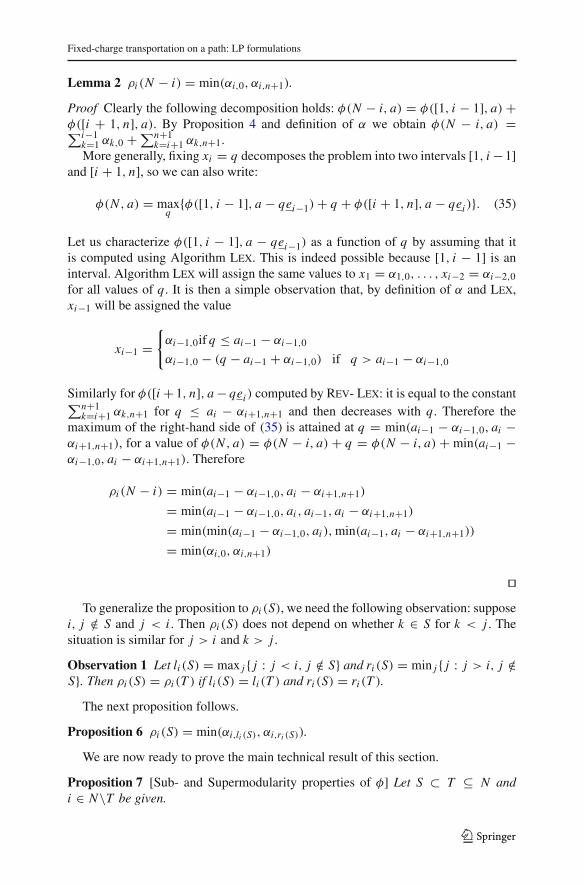
Lemma 2 ρi (N − i) = min(αi,0, αi,n+1).

Proof Clearly the following decomposition holds: φ(N − i, a) = φ([1, i − 1], a)+φ([i + 1, n], a). By Proposition 4 and definition of α we obtain φ(N − i, a) =∑i−1

k=1 αk,0 +∑n+1k=i+1 αk,n+1.

More generally, fixing xi = q decomposes the problem into two intervals [1, i −1]and [i + 1, n], so we can also write:

φ(N , a) = maxq{φ([1, i − 1], a − qei−1)+ q + φ([i + 1, n], a − qei )}. (35)

Let us characterize φ([1, i − 1], a − qei−1) as a function of q by assuming that itis computed using Algorithm Lex. This is indeed possible because [1, i − 1] is aninterval. Algorithm Lex will assign the same values to x1 = α1,0, . . . , xi−2 = αi−2,0for all values of q. It is then a simple observation that, by definition of α and Lex,xi−1 will be assigned the value

xi−1 ={

αi−1,0if q ≤ ai−1 − αi−1,0

αi−1,0 − (q − ai−1 + αi−1,0) if q > ai−1 − αi−1,0

Similarly for φ([i + 1, n], a− qei ) computed by Rev- Lex: it is equal to the constant∑n+1k=i+1 αk,n+1 for q ≤ ai − αi+1,n+1 and then decreases with q. Therefore the

maximum of the right-hand side of (35) is attained at q = min(ai−1 − αi−1,0, ai −αi+1,n+1), for a value of φ(N , a) = φ(N − i, a) + q = φ(N − i, a) + min(ai−1 −αi−1,0, ai − αi+1,n+1). Therefore

ρi (N − i) = min(ai−1 − αi−1,0, ai − αi+1,n+1)

= min(ai−1 − αi−1,0, ai , ai−1, ai − αi+1,n+1)

= min(min(ai−1 − αi−1,0, ai ), min(ai−1, ai − αi+1,n+1))

= min(αi,0, αi,n+1)

� To generalize the proposition to ρi (S), we need the following observation: suppose

i, j /∈ S and j < i . Then ρi (S) does not depend on whether k ∈ S for k < j . Thesituation is similar for j > i and k > j .

Observation 1 Let li (S) = max j { j : j < i, j /∈ S} and ri (S) = min j { j : j > i, j /∈S}. Then ρi (S) = ρi (T ) if li (S) = li (T ) and ri (S) = ri (T ).

The next proposition follows.

Proposition 6 ρi (S) = min(αi,li (S), αi,ri (S)).

We are now ready to prove the main technical result of this section.

Proposition 7 [Sub- and Supermodularity properties of φ] Let S ⊂ T ⊆ N andi ∈ N\T be given.

123

M. Van Vyve

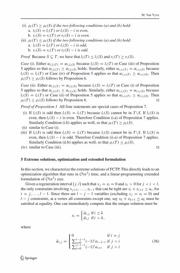
(i) ρi (T ) ≥ ρi (S) if the two following conditions (a) and (b) hold:a. li (S) = li (T ) or li (S)− i is even,b. ri (S) = ri (T ) or ri (S)− i is even.

(ii) ρi (T ) ≤ ρi (S) if the two following conditions (a) and (b) hold:a. li (S) = li (T ) or li (S)− i is odd,b. ri (S) = ri (T ) or ri (S)− i is odd.

Proof Because S ⊆ T , we have that li (T ) ≤ li (S) and ri (T ) ≥ ri (S).

Case (i). Either αi,li (T ) = αi,li (S) because li (S) = li (T ) or Case (iii) of Proposition5 applies so that αi,li (T ) ≥ αi,li (S) holds. Similarly, either αi,ri (T ) = αi,ri (S) becauseli (S) = li (T ) or Case (iv) of Proposition 5 applies so that αi,ri (T ) ≥ αi,ri (S). Thenρi (T ) ≥ ρi (S) follows by Proposition 6.

Case (ii). Either αi,li (T ) = αi,li (S) because li (S) = li (T ) or Case (i) of Proposition5 applies so that αi,li (T ) ≤ αi,li (S) holds. Similarly, either αi,ri (T ) = αi,ri (S) becauseli (S) = li (T ) or Case (ii) of Proposition 5 applies so that αi,ri (T ) ≤ αi,ri (S). Thenρi (T ) ≤ ρi (S) follows by Proposition 6. � Proof of Proposition 1 All four statements are special cases of Proposition 7.

(i) If li (S) is odd then li (S) = li (T ) because li (S) cannot be in T \S. If li (S) iseven, then li (S) − i is even. Therefore Condition (i.a) of Proposition 7 applies.Similarly Condition (i.b) applies as well, so that ρi (T ) ≥ ρi (S).

(ii) similar to Case (i).(iii) If li (S) is odd then li (S) = li (T ) because li (S) cannot be in T \S. If li (S) is

even, then li (S) − i is odd. Therefore Condition (ii.a) of Proposition 7 applies.Similarly Condition (ii.b) applies as well, so that ρi (T ) ≤ ρi (S).

(iv) similar to Case (iii). �

5 Extreme solutions, optimization and extended formulation

In this section, we characterize the extreme solutions of FCTP. This directly leads to anoptimization algorithm that runs in O(n3) time, and a linear-programming extendedformulation of O(n2) size.

Given a regeneration interval [ j, l] such that x j = xl = 0 and xi > 0 for j < i < l,the only constraints involving x j+1, . . . , xl−1 that can be tight are xi + xi+1 ≤ ai , fori = j, . . . , l − 1. Since there are l − j − 1 variables (excluding x j = xl = 0) andl − j constraints, at a vertex all constraints except one, say xk + xk+1 ≤ ak must besatisfied at equality. One can immediately compute that the unique solution must be

xi ={

αi, j if i ≤ kαi,l if i > k,

where

αi, j =⎧⎨

⎩

0 if i = j∑i− j−1t=0 (−1)t ai−1−t if j < i∑ j−i−1t=0 (−1)t ai+t if j > i

(36)

123

Fixed-charge transportation on a path: LP formulations

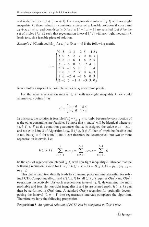
and is defined for i, j ∈ [0, n + 1]. For a regeneration interval [ j, l] with non-tightinequality k, these values xi constitute a piece of a feasible solution if constraintxk + xk+1 ≤ ak and bounds xi ≥ 0 for i ∈ [ j + 1, l − 1] are satisfied. Let F be theset of triples ( j, l, k) such that regeneration interval [ j, l] with non-tight inequality kleads to such a feasible piece of solution.

Example 1 [Continued] αi, j for i, j ∈ [0, n + 1] is the following matrix

α =

⎛

⎜⎜⎜⎜⎜⎜⎜⎜⎜⎜⎝

0 5 −3 3 −2 5 −1 25 0 8 2 7 0 6 33 8 0 6 1 8 2 53 −2 6 0 5 −2 4 12 7 −1 5 0 7 1 45 0 8 2 7 0 6 31 6 −2 4 −1 6 0 32 −3 5 −1 4 −3 3 0

⎞

⎟⎟⎟⎟⎟⎟⎟⎟⎟⎟⎠

Row i holds a superset of possible values of xi at extreme points.

For the same regeneration interval [ j, l] with non-tight inequality k, we couldalternatively define x ′ as

x ′i ={

αi, j if i ≤ kαi,l if i > k

In this case, the solution is feasible if x ′k + x ′k+1 ≤ ak only, because by construction ofα the other constraints are feasible. But note that x and x ′ will be identical whenever( j, k, l) ∈ F as this condition guarantees that xi is assigned the value ai−1 − xi−1and not ai in Line 3 of Algorithm Lex. If ( j, k, l) /∈ F , then x ′ might be feasible andx not, but x ′i = 0 for some i , and it can therefore be decomposed into two or moreregeneration intervals. Let

H( j, l, k) =k∑

i= j+1

piαi, j +l−1∑

i=k+1

piαi,l −l−1∑

i= j+1

fi

be the cost of regeneration interval [ j, l] with non-tight inequality k. Observe that thefollowing recursion is valid for k > j : H( j, l, k + 1) = H( j, l, k)+ pk+1(αk+1,l −αk+1, j ).

This characterization directly leads to a dynamic programming algorithm for solv-ing FCTP. Computing all αi, j and H( j, k, l) for all ( j, k, l) requires O(n2) and O(n3)

operations respectively. For each regeneration interval [ j, l], determining the mostprofitable and feasible non-tight inequality k and its associated profit H( j, l, k) canthen be performed in O(n) time. A standard O(n2) recursion for optimally decom-posing the interval [0, n + 1] into regeneration intervals completes the algorithm.Therefore we have the following proposition:

Proposition 8 An optimal solution of FCTP can be computed in O(n3) time.

123

M. Van Vyve

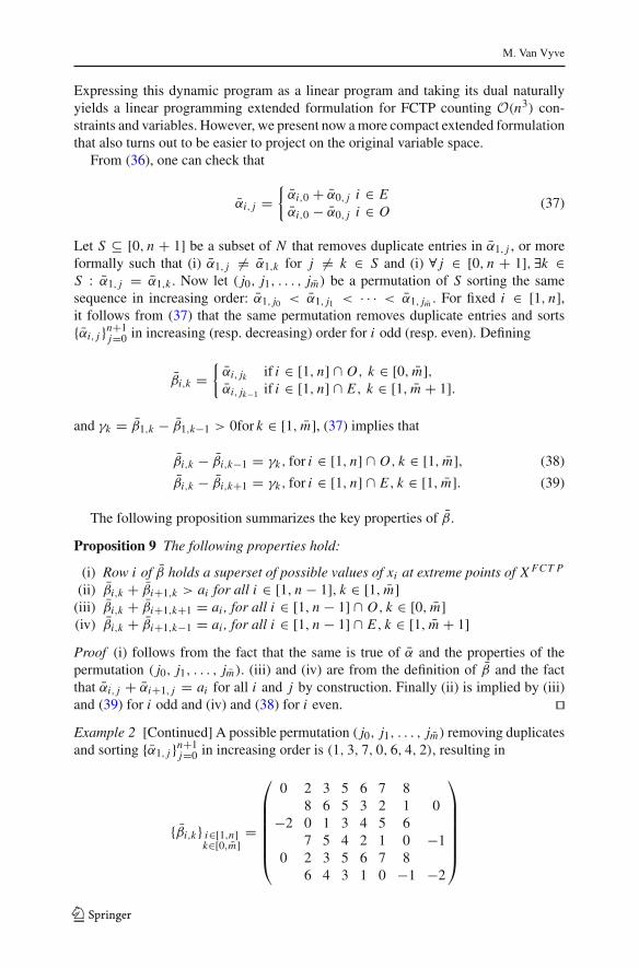
Expressing this dynamic program as a linear program and taking its dual naturallyyields a linear programming extended formulation for FCTP counting O(n3) con-straints and variables. However, we present now a more compact extended formulationthat also turns out to be easier to project on the original variable space.

From (36), one can check that

αi, j ={

αi,0 + α0, j i ∈ Eαi,0 − α0, j i ∈ O

(37)

Let S ⊆ [0, n + 1] be a subset of N that removes duplicate entries in α1, j , or moreformally such that (i) α1, j �= α1,k for j �= k ∈ S and (i) ∀ j ∈ [0, n + 1], ∃k ∈S : α1, j = α1,k . Now let ( j0, j1, . . . , jm) be a permutation of S sorting the samesequence in increasing order: α1, j0 < α1, j1 < · · · < α1, jm . For fixed i ∈ [1, n],it follows from (37) that the same permutation removes duplicate entries and sorts{αi, j }n+1

j=0 in increasing (resp. decreasing) order for i odd (resp. even). Defining

βi,k ={

αi, jk if i ∈ [1, n] ∩ O, k ∈ [0, m],αi, jk−1 if i ∈ [1, n] ∩ E, k ∈ [1, m + 1].

and γk = β1,k − β1,k−1 > 0for k ∈ [1, m], (37) implies that

βi,k − βi,k−1 = γk, for i ∈ [1, n] ∩ O, k ∈ [1, m], (38)

βi,k − βi,k+1 = γk, for i ∈ [1, n] ∩ E, k ∈ [1, m]. (39)

The following proposition summarizes the key properties of β.

Proposition 9 The following properties hold:

(i) Row i of β holds a superset of possible values of xi at extreme points of X FCT P

(ii) βi,k + βi+1,k > ai for all i ∈ [1, n − 1], k ∈ [1, m](iii) βi,k + βi+1,k+1 = ai , for all i ∈ [1, n − 1] ∩ O, k ∈ [0, m](iv) βi,k + βi+1,k−1 = ai , for all i ∈ [1, n − 1] ∩ E, k ∈ [1, m + 1]Proof (i) follows from the fact that the same is true of α and the properties of thepermutation ( j0, j1, . . . , jm). (iii) and (iv) are from the definition of β and the factthat αi, j + αi+1, j = ai for all i and j by construction. Finally (ii) is implied by (iii)and (39) for i odd and (iv) and (38) for i even. � Example 2 [Continued] A possible permutation ( j0, j1, . . . , jm) removing duplicatesand sorting {α1, j }n+1

j=0 in increasing order is (1, 3, 7, 0, 6, 4, 2), resulting in

{βi,k} i∈[1,n]k∈[0,m]

=

⎛

⎜⎜⎜⎜⎜⎜⎝

0 2 3 5 6 7 88 6 5 3 2 1 0

−2 0 1 3 4 5 67 5 4 2 1 0 −1

0 2 3 5 6 7 86 4 3 1 0 −1 −2

⎞

⎟⎟⎟⎟⎟⎟⎠

123

Fixed-charge transportation on a path: LP formulations

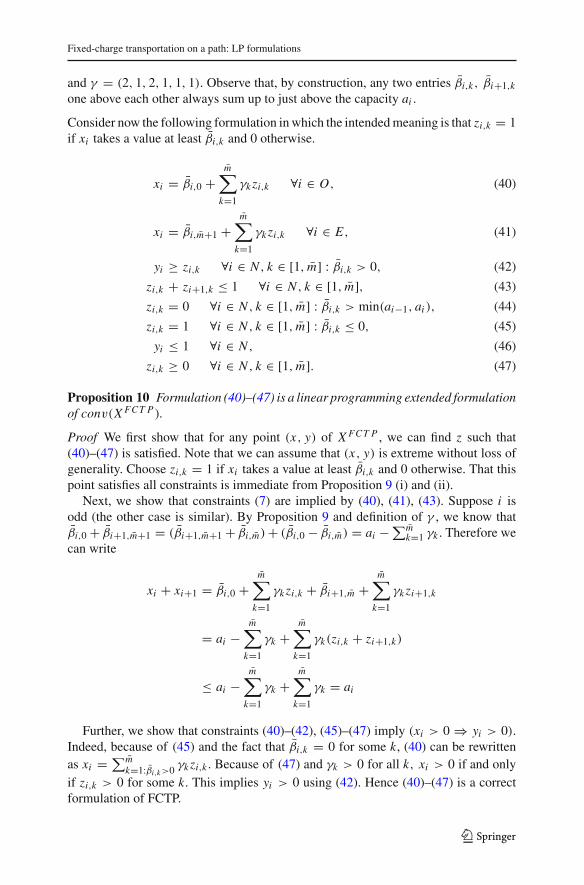
and γ = (2, 1, 2, 1, 1, 1). Observe that, by construction, any two entries βi,k, βi+1,k

one above each other always sum up to just above the capacity ai .

Consider now the following formulation in which the intended meaning is that zi,k = 1if xi takes a value at least βi,k and 0 otherwise.

xi = βi,0 +m∑

k=1

γk zi,k ∀i ∈ O, (40)

xi = βi,m+1 +m∑

k=1

γk zi,k ∀i ∈ E, (41)

yi ≥ zi,k ∀i ∈ N , k ∈ [1, m] : βi,k > 0, (42)

zi,k + zi+1,k ≤ 1 ∀i ∈ N , k ∈ [1, m], (43)

zi,k = 0 ∀i ∈ N , k ∈ [1, m] : βi,k > min(ai−1, ai ), (44)

zi,k = 1 ∀i ∈ N , k ∈ [1, m] : βi,k ≤ 0, (45)

yi ≤ 1 ∀i ∈ N , (46)

zi,k ≥ 0 ∀i ∈ N , k ∈ [1, m]. (47)

Proposition 10 Formulation (40)–(47) is a linear programming extended formulationof conv(X FCT P ).

Proof We first show that for any point (x, y) of X FCT P , we can find z such that(40)–(47) is satisfied. Note that we can assume that (x, y) is extreme without loss ofgenerality. Choose zi,k = 1 if xi takes a value at least βi,k and 0 otherwise. That thispoint satisfies all constraints is immediate from Proposition 9 (i) and (ii).

Next, we show that constraints (7) are implied by (40), (41), (43). Suppose i isodd (the other case is similar). By Proposition 9 and definition of γ , we know thatβi,0 + βi+1,m+1 = (βi+1,m+1 + βi,m)+ (βi,0 − βi,m) = ai −∑m

k=1 γk . Therefore wecan write

xi + xi+1 = βi,0 +m∑

k=1

γk zi,k + βi+1,m +m∑

k=1

γk zi+1,k

= ai −m∑

k=1

γk +m∑

k=1

γk(zi,k + zi+1,k)

≤ ai −m∑

k=1

γk +m∑

k=1

γk = ai

Further, we show that constraints (40)–(42), (45)–(47) imply (xi > 0⇒ yi > 0).Indeed, because of (45) and the fact that βi,k = 0 for some k, (40) can be rewrittenas xi =∑m

k=1:βi,k>0 γk zi,k . Because of (47) and γk > 0 for all k, xi > 0 if and onlyif zi,k > 0 for some k. This implies yi > 0 using (42). Hence (40)–(47) is a correctformulation of FCTP.

123

M. Van Vyve

It remains to see that, by the change of variables z′i,k = −zi,k and y′i = −yi for ieven and z′i,k = zi,k and y′i = yi for i odd, each constraint (42), (43) becomes a boundon a difference of two variables. The matrix associated to this modified constraintsystem is therefore a network flow matrix and therefore extreme points of (40)–(47)have y and z integer-valued. The result follows. �

At the end of Sect. 2, we argued that BBLS can be modelled as FCT with additionalconstraints equalizing some setup variables. Therefore we are interested in studyingthe polyhedral impact of the addition this type of constraints. The following corollarysheds some light on this question for FCTP.

Corollary 2 conv(X FCT P ) intersected with constraints of the form yi − y j ≤ dwhere i and j have the same parity and d is integral is an integral polyhedron.

Note that each constraint (26) links the setup variables of two arcs incident to the samenode, and therefore of two arcs that are at an odd distance from each other. Thereforethe corollary does not apply.

6 Projection

A linear programming extended formulation automatically leads to a characterizationof the convex hull of the solution in the original space of variables through projection.Indeed, testing if a point (x∗, y∗) satisfying y∗ ≤ 1 belongs to conv(X FCT P ) isequivalent to testing whether the following LP in variables z is feasible:

max 0,∑

k∈Ki

γk zi,k = x∗i ∀i ∈ N , (�i )

zi,k ≤ y∗i ∀i ∈ N , k ∈ Ki , (δi,k)

zi,k + zi+1,k ≤ 1 ∀i ∈ [1, n − 1], k ∈ Ki ∩ Ki+1, (ρi,k)

zi,k ≥ 0 ∀i ∈ N , k ∈ Ki ,

where Ki = {k ∈ [1, m] : 0 < βi,k ≤ min(ai−1, ai )}. Through LP duality, this isequivalent to testing whether the following LP is bounded:

minn∑

i=1

x∗i �i +n∑

i=1

∑

k∈Ki

y∗i δi,k +n−1∑

i=1

∑

k∈Ki∩Ki+1

ρi,k,

γk�i + δi,k + ρi−1,k + ρi,k ≥ 0 ∀i ∈ N , k ∈ Ki ,

ρi,k = 0 ∀i /∈ [1, n − 1]or k /∈ Ki ∩ Ki+1,

δ, ρ ≥ 0.

Dividing the constraint by γk and rescaling δi,k and ρi,k by γk , one obtains the equiv-alent LP

123

Fixed-charge transportation on a path: LP formulations

minn∑

i=1

x∗i �i +n∑

i=1

∑

k∈Ki

γk y∗i δi,k +n−1∑

i=1

∑

k∈Ki∩Ki+1

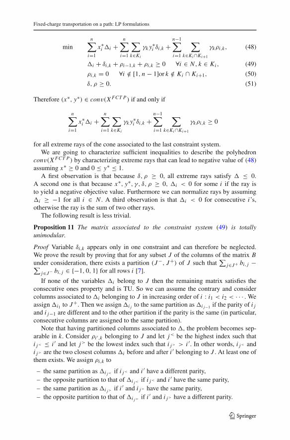
γkρi,k, (48)

�i + δi,k + ρi−1,k + ρi,k ≥ 0 ∀i ∈ N , k ∈ Ki , (49)

ρi,k = 0 ∀i /∈ [1, n − 1]or k /∈ Ki ∩ Ki+1, (50)

δ, ρ ≥ 0. (51)

Therefore (x∗, y∗) ∈ conv(X FCT P ) if and only if

n∑

i=1

x∗i �i +n∑

i=1

∑

k∈Ki

γk y∗i δi,k +n−1∑

i=1

∑

k∈Ki∩Ki+1

γkρi,k ≥ 0

for all extreme rays of the cone associated to the last constraint system.We are going to characterize sufficient inequalities to describe the polyhedron

conv(X FCT P ) by characterizing extreme rays that can lead to negative value of (48)assuming x∗ ≥ 0 and 0 ≤ y∗ ≤ 1.

A first observation is that because δ, ρ ≥ 0, all extreme rays satisfy � ≤ 0.A second one is that because x∗, y∗, γ, δ, ρ ≥ 0, �i < 0 for some i if the ray isto yield a negative objective value. Furthermore we can normalize rays by assuming�i ≥ −1 for all i ∈ N . A third observation is that �i < 0 for consecutive i’s,otherwise the ray is the sum of two other rays.

The following result is less trivial.

Proposition 11 The matrix associated to the constraint system (49) is totallyunimodular.

Proof Variable δi,k appears only in one constraint and can therefore be neglected.We prove the result by proving that for any subset J of the columns of the matrix Bunder consideration, there exists a partition (J−, J+) of J such that

∑j∈J+ bi, j −∑

j∈J− bi, j ∈ {−1, 0, 1} for all rows i [7].

If none of the variables �i belong to J then the remaining matrix satisfies theconsecutive ones property and is TU. So we can assume the contrary and considercolumns associated to �i belonging to J in increasing order of i : i1 < i2 < · · · . Weassign �i1 to J+. Then we assign �i j to the same partition as �i j−1 if the parity of i j

and i j−1 are different and to the other partition if the parity is the same (in particular,consecutive columns are assigned to the same partition).

Note that having partitioned columns associated to �, the problem becomes sep-arable in k. Consider ρi ′,k belonging to J and let j< be the highest index such thati j< ≤ i ′ and let j> be the lowest index such that i j> > i ′. In other words, i j< andi j> are the two closest columns �i before and after i ′ belonging to J . At least one ofthem exists. We assign ρi,k to

– the same partition as �i j< if i j< and i ′ have a different parity,– the opposite partition to that of �i j< if i j< and i ′ have the same parity,– the same partition as �i j> if i ′ and i j> have the same parity,– the opposite partition to that of �i j> if i ′ and i j> have a different parity.

123

M. Van Vyve

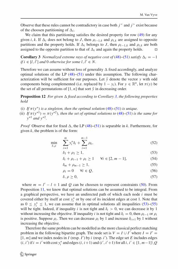
Observe that these rules cannot be contradictory in case both j< and j> exist becauseof the choosen partitioning of �i .

We claim that this partitioning satisfies the desired property for row (49) for anygiven i, k. If �i does not belong to J , then ρi−1,k and ρi,k are assigned to oppositepartitions and the property holds. If �i belongs to J , then ρi−1,k and ρi,k are bothassigned to the opposite partition to that of �i and again the property holds. � Corollary 3 Normalized extreme rays of negative cost of (48)–(51) satisfy �i = −1if i ∈ [l, l ′] and 0 otherwise for some l, l ′ ∈ N.

Therefore we can assume without loss of generality � fixed accordingly, and analyzeoptimal solutions of the LP (48)–(51) under this assumption. The following char-acterization will be sufficient for our purposes. Let y denote the vector y with oddcomponents being complemented (i.e. replaced by 1 − yi ). For y ∈ R

n , let π(y) bethe set of all permutations of [1, n] that sort y in decreasing order.

Proposition 12 For given � fixed according to Corollary 3, the following propertieshold

(i) If π(y∗) is a singleton, then the optimal solution (48)–(51) is unique.(ii) If π(y∗1) = π(y∗2), then the set of optimal solutions to (48)–(51) is the same for

y∗1 and y∗2.

Proof Observe that for fixed �, the LP (48)–(51) is separable in k. Furthermore, forgiven k, the problem is of the form:

minδ,ρ

m∑

i=1

y∗i δi +m−1∑

i=1

ρk, (52)

δ1 + ρ1 ≥ 1, (53)

δi + ρi−1 + ρi ≥ 1 ∀i ∈ [2, m − 1], (54)

δm + ρm−1 ≥ 1, (55)

ρi = 0 ∀i ∈ Q, (56)

δ, ρ ≥ 0, (57)

where m = l ′ − l + 1 and Q can be choosen to represent constraints (50). FromProposition 11, we know that optimal solutions can be assumed to be integral. Froma graphical perspective, we have an undirected path of which each node i must becovered either by itself at cost y∗i or by one of its incident edges at cost 1. Note thatas 0 ≤ y∗i ≤ 1, we can assume that in optimal solutions all inequalities (53)–(55)will be tight. Indeed, if inequality i is not tight and δi > 0, we can decrease it by 1without increasing the objective. If inequality i is not tight and δi = 0, then ρi−1 or ρi

is positive. Suppose ρi . Then we can decrease ρi by 1 and increase δi+1 by 1 withoutincreasing the objective.

Therefore the same problem can be modelled as the more classical perfect matchingproblem in the following bipartite graph. The node set is V = I ∪ I ′ where I = I ′ =[1, m] and we index nodes in I (resp. I ′) by i (resp. i ′). The edge set E includes edges(i, i ′) if i = i ′with cost y∗i and edges (i, i+1) and (i ′, i ′+1) for all i, i ′ ∈ [1, m−1]\Q

123

Fixed-charge transportation on a path: LP formulations

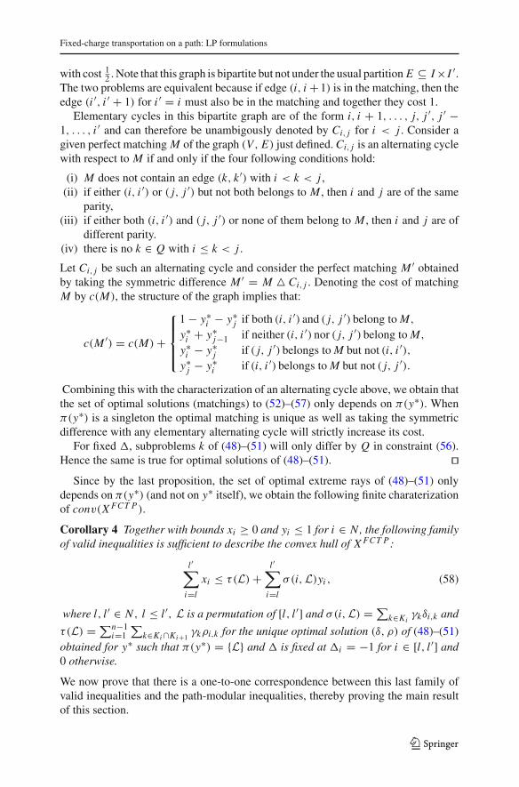
with cost 12 . Note that this graph is bipartite but not under the usual partition E ⊆ I× I ′.

The two problems are equivalent because if edge (i, i +1) is in the matching, then theedge (i ′, i ′ + 1) for i ′ = i must also be in the matching and together they cost 1.

Elementary cycles in this bipartite graph are of the form i, i + 1, . . . , j, j ′, j ′ −1, . . . , i ′ and can therefore be unambigously denoted by Ci, j for i < j . Consider agiven perfect matching M of the graph (V, E) just defined. Ci, j is an alternating cyclewith respect to M if and only if the four following conditions hold:

(i) M does not contain an edge (k, k′) with i < k < j ,(ii) if either (i, i ′) or ( j, j ′) but not both belongs to M , then i and j are of the same

parity,(iii) if either both (i, i ′) and ( j, j ′) or none of them belong to M , then i and j are of

different parity.(iv) there is no k ∈ Q with i ≤ k < j .

Let Ci, j be such an alternating cycle and consider the perfect matching M ′ obtainedby taking the symmetric difference M ′ = M � Ci, j . Denoting the cost of matchingM by c(M), the structure of the graph implies that:

c(M ′) = c(M)+

⎧⎪⎪⎨

⎪⎪⎩

1− y∗i − y∗j if both (i, i ′) and ( j, j ′) belong to M,

y∗i + y∗j−1 if neither (i, i ′) nor ( j, j ′) belong to M,

y∗i − y∗j if ( j, j ′) belongs to M but not (i, i ′),y∗j − y∗i if (i, i ′) belongs to M but not ( j, j ′).

Combining this with the characterization of an alternating cycle above, we obtain thatthe set of optimal solutions (matchings) to (52)–(57) only depends on π(y∗). Whenπ(y∗) is a singleton the optimal matching is unique as well as taking the symmetricdifference with any elementary alternating cycle will strictly increase its cost.

For fixed �, subproblems k of (48)–(51) will only differ by Q in constraint (56).Hence the same is true for optimal solutions of (48)–(51). �

Since by the last proposition, the set of optimal extreme rays of (48)–(51) onlydepends on π(y∗) (and not on y∗ itself), we obtain the following finite charaterizationof conv(X FCT P ).

Corollary 4 Together with bounds xi ≥ 0 and yi ≤ 1 for i ∈ N, the following familyof valid inequalities is sufficient to describe the convex hull of X FCT P :

l ′∑

i=l

xi ≤ τ(L)+l ′∑

i=l

σ(i,L)yi , (58)

where l, l ′ ∈ N , l ≤ l ′, L is a permutation of [l, l ′] and σ(i,L) =∑k∈Ki

γkδi,k and

τ(L) =∑n−1i=1

∑k∈Ki∩Ki+1

γkρi,k for the unique optimal solution (δ, ρ) of (48)–(51)obtained for y∗ such that π(y∗) = {L} and � is fixed at �i = −1 for i ∈ [l, l ′] and0 otherwise.

We now prove that there is a one-to-one correspondence between this last family ofvalid inequalities and the path-modular inequalities, thereby proving the main resultof this section.

123

M. Van Vyve

Proposition 13 Together with bounds xi ≥ 0 and yi ≤ 1 for i ∈ N, the path-modularinequalities are sufficient to describe the convex hull of X FCT P .

Proof Let l, l ′ ∈ N , l ≤ l ′ and a permutation L of [l, l ′] be given. Consider any of the|l ′ − l+2| points (xk, yk) of Proposition 2 for the ordering ( j1, j2, . . . , jn) = L. Sucha point lies on the boundary of conv(X FCT P ), and therefore a separation algorithmthat maximizes the violation will output a valid inequality that is tight at this point.Consider now the LP (48)–(51) with � fixed at �i = −1 for l ≤ i ≤ l ′ and 0 otherwise.This LP actually determines a valid inequality of the form

∑l ′i=l xi ≤ π0+∑l ′

i=l πi yi

maximizing the violation. Now observe that the permutation L sorts yk in decreasingorder for any k. Therefore the corresponding inequality (58) is tight at (xk, yk) for anyk. By Proposition 2, this is also the case for the path-modular inequality associated to(l, l ′,L). As these |l ′ − l + 2| points are affinely independent, these two inequalitiesare identical. �

We now turn to the question of separating a point (x∗, y∗) with x∗i ≥ 0 and y∗i ≤ 1for all i ∈ N from the polyhedron defined by the path-modular inequalities. It followsdirectly from Proposition 12 that the ordering maximizing the violation sorts y∗ indecreasing order. Moreover this ordering is independent of L .

Computing all αi, j can be done in O(n2) by n calls to Lex and n calls toRev- Lex. Finally, for each L and given the ordering L, computing each coefficient ofthe path-modular inequality can be done in constant time provided li (OL ∪ Ei

L\OiL)

and ri (OL ∪ EiL\Oi

L) are available. Because, for L = [k, p],

li (OL ∪ EiL\Oi

L) = max(

k, li (ON ∪ EiN\Oi

N ))

and

ri (OL ∪ EiL\Oi

L) = min(

p, ri (ON ∪ EiN\Oi

N ))

computing these can be done once for all L in O(n2) operations. To summarize, wehave proved the following result:

Proposition 14 The separation problem associated with the path-modular inequali-ties can be solved in O(n3) time.

In practice, it is unlikely that path-modular inequalities for very large intervals L will benecessary. So it is interesting to consider separating “short” path-modular inequalities.In fact, a similar analysis yields the following result.

Proposition 15 The separation problem associated with the path-modular inequali-ties with |L| ≤ k can be solved in O(n2 + k2n) time.

7 Facets of small instances

Appendix 9.1 lists all facets of Example 1 and give their construction as path-modularinequalities.

We also enumerated all facets of an instance of a fixed-charge transportation prob-lem (2)–(5) of size 3×2 with data C = [4, 5, 3] and D = [8, 6]. There are 136 facets,

123

Fixed-charge transportation on a path: LP formulations

of which 19 are trivial (one of the inequalities (2)–(5). Seven facets correspond to flowcover or path-modular inequalities of length 2 (they are identical in this case). Six facetsare facets of a single-node flow relaxation of size 3 (flow cover, lifted flow cover orother inequalities). Eight facets are path-modular inequalities of size 3 and three facetsare path-modular inequalities of size 4. The other 93 facets have edges with non-zerocoefficients that are not stars (flow covers) or paths (path-modular inequalities).

This indicates that the path-modular inequalities capture some of the combinatorialstructure of this more general problem as well.

8 Conclusion

This paper is a polyhedral analysis of the Fixed-Charge Transportation problem onPaths (FCTP). The aim of this study is to improve our ability to solve the Fixed-ChargeTransportation problem on general bipartite graphs, and the even more general BigBucket Lot-Sizing problem.

For FCTP, we characterize extreme points, we give a O(n3) algorithm and twocompact linear programming extended formulations. We describe a new family ofvalid inequalities that are shown to describe the convex hull of the solutions to FCTP,and that can be separated in O(n3) time. We also report computational results showingthat the extended formulation is most efficient for solving instances of FCTP becausenot too many additional variables and constraints are necessary in practice. Theseexperiments also illustrate that “short” path-modular inequalities are usually sufficientto obtain excellent bounds. Finally, we show through an example that a number offacet-defining inequalities for FCT are path-modular inequalities of path relaxations.

This work can be pursued in many directions. Among the 93 unexplained facetsdiscussed in Sect. 7, 4 of them seem to generalize path-modular inequalities for cycles.Indeed, they have coefficients 0 or 1 for variables xi , and their support correspondsto a cycle of size 4 (instead of a path for path-modular inequalities). Moreover thecoefficients of variables yi are exactly of the form (33) for some permutation of theedges, with the set functions φ and ρi naturally interpreted for cycles. This wouldcomplete the study of fixed-charge transportation on graphs of node degree at most 2.

This in turns raises the question of generalizing path-modular inequalities to othergraph structures. In particular, it would be nice to be able to describe a family of inequal-ities that subsumes path-modular (paths) and simple flow-cover inequalities (stars).

Another question is whether path-modular inequalities can be adapted to deal withcapacities on the edges and/or setup variables on the nodes. From the point of viewof [4], a generalization of our work would be to study mixing sets linked by a path ofwhich each edge is arbitrarily directed.

From a computational point of view, we would like to improve the running timeof the separation algorithm for path-modular inequalities. In particular one could tryto exploit the similarity between two inequalities associated to intervals differing byone element. If one wants to use the present work to better solve general fixed-chargetransportation problems, the crucial step will be to determine path relaxations thatgenerate violated path-modular inequalities. This is not a trivial task.

Acknowledgments The author is grateful to L.A. Wolsey for commenting an earlier version of this text.

123

M. Van Vyve

9 Appendix

9.1 Facets of Example 1

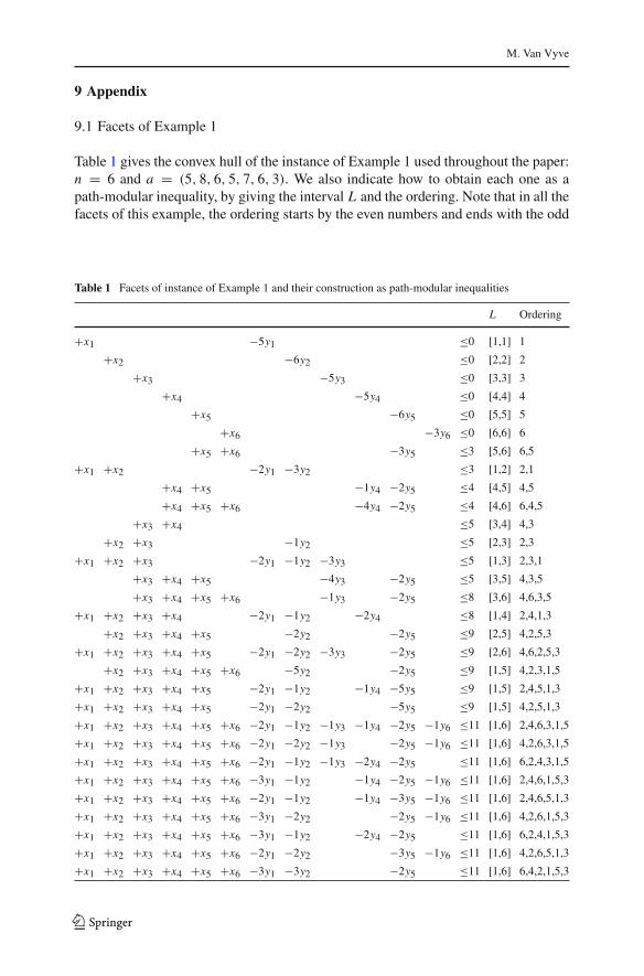
Table 1 gives the convex hull of the instance of Example 1 used throughout the paper:n = 6 and a = (5, 8, 6, 5, 7, 6, 3). We also indicate how to obtain each one as apath-modular inequality, by giving the interval L and the ordering. Note that in all thefacets of this example, the ordering starts by the even numbers and ends with the odd

Table 1 Facets of instance of Example 1 and their construction as path-modular inequalities

L Ordering

+x1 −5y1 ≤0 [1,1] 1

+x2 −6y2 ≤0 [2,2] 2

+x3 −5y3 ≤0 [3,3] 3

+x4 −5y4 ≤0 [4,4] 4

+x5 −6y5 ≤0 [5,5] 5

+x6 −3y6 ≤0 [6,6] 6

+x5 +x6 −3y5 ≤3 [5,6] 6,5

+x1 +x2 −2y1 −3y2 ≤3 [1,2] 2,1

+x4 +x5 −1y4 −2y5 ≤4 [4,5] 4,5

+x4 +x5 +x6 −4y4 −2y5 ≤4 [4,6] 6,4,5

+x3 +x4 ≤5 [3,4] 4,3

+x2 +x3 −1y2 ≤5 [2,3] 2,3

+x1 +x2 +x3 −2y1 −1y2 −3y3 ≤5 [1,3] 2,3,1

+x3 +x4 +x5 −4y3 −2y5 ≤5 [3,5] 4,3,5

+x3 +x4 +x5 +x6 −1y3 −2y5 ≤8 [3,6] 4,6,3,5

+x1 +x2 +x3 +x4 −2y1 −1y2 −2y4 ≤8 [1,4] 2,4,1,3

+x2 +x3 +x4 +x5 −2y2 −2y5 ≤9 [2,5] 4,2,5,3

+x1 +x2 +x3 +x4 +x5 −2y1 −2y2 −3y3 −2y5 ≤9 [2,6] 4,6,2,5,3

+x2 +x3 +x4 +x5 +x6 −5y2 −2y5 ≤9 [1,5] 4,2,3,1,5

+x1 +x2 +x3 +x4 +x5 −2y1 −1y2 −1y4 −5y5 ≤9 [1,5] 2,4,5,1,3

+x1 +x2 +x3 +x4 +x5 −2y1 −2y2 −5y5 ≤9 [1,5] 4,2,5,1,3

+x1 +x2 +x3 +x4 +x5 +x6 −2y1 −1y2 −1y3 −1y4 −2y5 −1y6 ≤11 [1,6] 2,4,6,3,1,5

+x1 +x2 +x3 +x4 +x5 +x6 −2y1 −2y2 −1y3 −2y5 −1y6 ≤11 [1,6] 4,2,6,3,1,5

+x1 +x2 +x3 +x4 +x5 +x6 −2y1 −1y2 −1y3 −2y4 −2y5 ≤11 [1,6] 6,2,4,3,1,5

+x1 +x2 +x3 +x4 +x5 +x6 −3y1 −1y2 −1y4 −2y5 −1y6 ≤11 [1,6] 2,4,6,1,5,3

+x1 +x2 +x3 +x4 +x5 +x6 −2y1 −1y2 −1y4 −3y5 −1y6 ≤11 [1,6] 2,4,6,5,1,3

+x1 +x2 +x3 +x4 +x5 +x6 −3y1 −2y2 −2y5 −1y6 ≤11 [1,6] 4,2,6,1,5,3

+x1 +x2 +x3 +x4 +x5 +x6 −3y1 −1y2 −2y4 −2y5 ≤11 [1,6] 6,2,4,1,5,3

+x1 +x2 +x3 +x4 +x5 +x6 −2y1 −2y2 −3y5 −1y6 ≤11 [1,6] 4,2,6,5,1,3

+x1 +x2 +x3 +x4 +x5 +x6 −3y1 −3y2 −2y5 ≤11 [1,6] 6,4,2,1,5,3

123

Fixed-charge transportation on a path: LP formulations

numbers. This means that these facets are all tight at a point where all edges are open.There are instances of FCTP for which path-modular inequalities are facets and donot satisfy this property.

References

1. Aardal, K.: Capacitated facility location: separation algorithms and computational experience. Math.Program. A 81, 149–175 (1998)

2. Akartunal, K., Miller, A.J.: A Computational analysis of lower bounds for big bucket productionplanning problems. Optimization. http://www.optimization-online.org/DB_FILE/2007/05/1668.pdf(2007)

3. Carr, R., Fleischer, L., Leung, V., Phillips, C.: Strengthening integrality gaps for capacitated networkdesign and covering problems. In: Proceedings of the 11th Annual ACM-SIAM Symposium on DiscreteAlgorithms, pp. 106–115 (2000)

4. Conforti, M., Di Summa, M., Eisenbrand, F., Wolsey, L.A.: Network formulations of mixed-integerprograms. Math. Oper. Res. 34, 194–209 (2009)

5. Conforti, M., Wolsey, L.A., Zambelli, G.: Projecting an extended formulation for mixed-integer coverson bipartite graphs. Math. Oper. Res. 35, 603–623 (2010)

6. Di Summa, M., Wolsey, L.A.: Mixing sets linked by bidirected paths. CORE Discussion Paper 2010/61,Louvain-la-Neuve (2010)

7. Ghouila-Houri, A.: Caracterisation des matrices totalement unimodulaires. CR Acad. Sci. Paris 254,1192–1194 (1962)

8. Gu, Z., Nemhauser, G.L., Savelsbergh, M.W.P.: Lifted flow cover inequalities for mixed 0–1 integerprograms. Math. Program. A 85, 439–467 (1999)

9. Jans, R., Degraeve, Z.: Improved lower bounds for the capacitated lot sizing problem with setup times.Oper. Res. Lett. 32, 185–195 (2004)

10. Krarup, J., Bilde, O.: Plant location, set covering and economic lotsizes: an O(mn) algorithm forstructured problems. In: Collatz, L. (ed.) Optimierung bei Graphentheoretischen und GanzzahligenProbleme, pp. 155–180. Birkhauser Verlag, Basel (1977)

11. Miller, A.J., Nemhauser, G.L., Savelsbergh, M.W.P.: On the polyhedral structure of a multi-item pro-duction planning model with setup times. Math. Program. 94(2–3), 375–405 (2003)

12. Padberg, M.W., van Roy, T.J., Wolsey, L.A.: Valid linear inequalities for fixed charge problems. Oper.Res. 33, 842–861 (1985)

13. Trigeiro, W.W., Thomas, L.J., McClain, J.O.: Capacitated lot sizing with setup times. Manage. Sci.35(3), 353–366 (1989)

14. van Roy, T.J., Wolsey, L.A.: Solving mixed integer programming problems using automatic reformu-lation. Oper. Res. 33, 45–57 (1987)

15. Van Vyve, M., Wolsey, L.A.: Approximate extended formulations. Math. Programm. B 105, 501–522(2006)

16. Wolsey, L.A.: Submodularity and valid inequalities in capacitated fixed charge networks. Oper. Res.Lett. 8(3), 119–124 (1989)

123