Five Ways in Which Computational Modeling Can Help Advance

Topics in Cognitive Science 12 (2020) 925–941© 2019 The Authors. Topics in Cognitive Science published by Wiley Periodicals, Inc. on behalf of CognitiveScience SocietyISSN:1756-8765 onlineDOI: 10.1111/tops.12474

This article is part of the topic “Learning Grammatical Structures: Developmental, Cross-species and Computational Approaches,” Carel ten Cate, Clara Levelt, Judit Gervain, ChrisPetkov, and Willem Zuidema (Topic Editors). For a full listing of topic papers, see http://onlinelibrary.wiley.com/journal/10.1111/(ISSN)1756-8765/earlyview

Five Ways in Which Computational Modeling Can HelpAdvance Cognitive Science: Lessons From Artificial

Grammar Learning

Willem Zuidema,a Robert M. French,b Raquel G. Alhama,c Kevin Ellis,d

Timothy J. O’Donnell,e Tim Sainburg,f Timothy Q. Gentnerg

aInstitute for Logic, Language and Computation, University of AmsterdambLEAD-CNRS, University of Burgundy,

cMax Planck Institute for PsycholinguisticsdDepartment of Brain and Cognitive Sciences, MIT

eDepartment of Linguistics, McGill UniversityfDepartment of Psychology, University of California San Diego

gDepartment of Psychology & Division of Biological Sciences, University of California San Diego

Received 19 April 2018; received in revised form 17 June 2019; accepted 24 June 2019

Abstract

There is a rich tradition of building computational models in cognitive science, but modeling,

theoretical, and experimental research are not as tightly integrated as they could be. In this paper,

we show that computational techniques—even simple ones that are straightforward to use—can

greatly facilitate designing, implementing, and analyzing experiments, and generally help lift

research to a new level. We focus on the domain of artificial grammar learning, and we give five

concrete examples in this domain for (a) formalizing and clarifying theories, (b) generating stim-

uli, (c) visualization, (d) model selection, and (e) exploring the hypothesis space.

Correspondence should be sent to Willem Zuidema, Institute for Logic, Language and Computation,

University of Amsterdam, 1098 XG Amsterdam, The Netherlands. E-mail: [email protected]

This is an open access article under the terms of the Creative Commons Attribution License, which

permits use, distribution and reproduction in any medium, provided the original work is properly cited.

http://onlinelibrary.wiley.com/journal/10.1111/(ISSN)1756-8765/earlyview

http://onlinelibrary.wiley.com/journal/10.1111/(ISSN)1756-8765/earlyview

mailto:

Keywords: Computational modeling; Neural networks; Formal grammars; Bayesian modeling;

Artificial language learning; Artificial grammar learning

1. Introduction

Computer models have given us a better understanding of everything from the evolu-

tion of stars to the evolution of the human eye, from chemical reactions in the ozone

layer to animal mating behavior, and much more. Over the years many computational

models have been developed for the study of cognition. The first computer model (Roche-

ster et al., 1956) of category learning had of a total of 69 “artificial neurons” and cranked

out its calculations at the rate of 5,000 computations/second (compared to 93 9 1015

computations/second for the fastest computer today). Many models have been developed

since, contributing to a better understanding of some of the processes underlying human

cognition. If nothing else, they revealed human cognition to be far more difficult to simu-

late computationally than had been previously suspected.

Despite this long history in cognitive science, computational modeling is not uncontro-

versial. Computational modeling sometimes appears as an inward looking field—a

domain separated from experimental research, where obscure technical details dominate,

hungry for data but seldom giving something back. Modeling, in that view, is a post hoc

process, taking place after data collection and, at best, providing an implementation of

explanatory theories of experimental results.

However, this is not how things need to be. Computational techniques, even simple

ones that are straightforward to use, can greatly facilitate designing, implementing, and

analyzing experiments, and generally help lift research to a new level. In this paper, we

give five concrete examples of how computational models can help design and implement

experiments, as well as help in analyzing and interpreting the results. We focus on the

domain of Artificial Grammar Learning (AGL), a field that employs artificial language

stimuli to systematically manipulate certain factors to test for language learning. AGL is

a particularly illustrative case because the design of artificial stimuli capturing particular

features of natural language, while ruling out other interpretations, is particularly chal-

lenging. It is also a field where many of the same types of debates have happened as in

cognitive science at large, and where many of the different computational modeling para-

digms have been applied (e.g., Alhama & Zuidema, 2017, 2019; Culbertson et al., 2013;

Frank et al., 2010; French et al., 2011; Gagliardi et al., 2017; Kemp et al., 2007; Kirby

et al., 2015; Marcus et al., 1999; Pearl et al., 2010; Perruchet et al., 2006; Wonnacott,

2011).

In the remainder of this paper, we will discuss our examples in an order that roughly

follows the experimental cycle. We start where, ideally, all research starts, with rival the-

ories on the cognitive processes underlying grammar learning. In Section 2, we discuss

how models can be used to formalize and clarify theories. In Section 3, we shift to imple-

mentations of concrete experiments. As computational tools for generating stimuli,

926 W. Zuidema et al. / Topics in Cognitive Science 12 (2020)

presenting stimuli, and recording responses are well-known, we focus on the use of com-

putational techniques for selecting and randomizing stimuli and for avoiding confounds in

the experimental design. When the data are collected, the next task is to analyze and

report the results. In Section 4, we discuss modern computational techniques, such as

those coming out of the deep learning field, that go beyond such standard reporting and

visualization techniques, and offer great insight into the cognitive systems under study. In

Section 5, we discuss the use of model selection techniques for exploratory data analysis

that allows one to uncover patterns in the data not easily discernible without computa-

tional modeling techniques. Finally, in Section 6, we discuss how a system based on

Bayesian Program Learning can be used to explore a space of hypotheses, by generating

and visualizing alternative hypotheses on strategies that participants in an AGL experi-

ment might follow.

2. Formalization

One of the most important uses of computational techniques is to define formal,

explanatory models. In this section, we will illustrate the benefits of having a formal and

computationally implemented model available, using the “word segmentation” phe-

nomenon, from artificial language learning, as our running example. We know that chil-

dren as young as 2 months of age can segment “words” from a continuous syllable or

image stream devoid of any markers indicating word boundaries and that they can do this

without recourse to semantics. How?

There are two main, and conflicting, views of how infants do this. The first says that

they have a mechanism that is sensitive to the probabilities of hearing one syllable and

expecting it to be followed by another (i.e., Transitional Probabilities). Boundaries

between words are where these probabilities are lowest. Another view says that infants

remember hearing certain pairs of syllables (“chunks”) better than other pairs because

they occurred more frequently in the syllable stream. They automatically build internal

representations of these frequently heard pairs and incorporate these internal representa-

tions to build larger syllable chunks.Both views make intuitive sense and rely on a body of empirical work. Formal model-

ing can help in evaluating which of the views provide a better explanation for the empiri-

cal record as a whole, by first making both views more precise, by evaluating whether

they qualitatively reproduce the data equally well, and by deriving new testable predic-

tions.

The Transitional Probability view has been formalized by the well-known Simple

Recurrent Network (SRN) of Elman (1990). Formalizing the alternate Implicit Chunk

Recognition view has yielded a model called TRACX2 (initially introduced by French &

Cottrell, 2014, and based on an earlier version of the same architecture: TRACX; French

et al., 2011). Both models can be used to fulfill the task of segmenting sequences of

sounds, images, movements, and so on into “words,” in a bottom-up manner. And both

the SRN and TRACX2, it turns out, can successfully reproduce existing data when tested

W. Zuidema et al. / Topics in Cognitive Science 12 (2020) 927

on syllable streams such as those used in early infant artificial language learning experi-

ments (e.g., see Mareschal & French, 2017).

We will not discuss details of SRNs or TRACX2 here (Fig. 1 gives a succinct descrip-

tion of TRACX2). One important aspect of both models is that they receive information

item-by-item and try to integrate the new information with information from previous

items in a compressed representation: the hidden layer. SRNs are typically trained to pre-

dict the next item based on their output; TRACX2, in contrast, attempts to reproduce the

current input based on its output.

TRACX2 is thus a recurrent, autoencoder network (“recurrent” means that it processes

sequences item-by-item, and information from previous time steps stays in the network

through recurrent connections; “Autoencoder” means that it is trained to produce on out-

put what appears on input).

Crucially, if TRACX2 is successful (low reproduction error), much of the compressed rep-

resentation will be maintained for the next time step. If the reproduction error is high, most of

the compressed representation is discarded. Key to understanding the model’s behavior is the

observation that if at time t, the reproduction error (Dt) is small, this could only have occurred

if the network has seen the two items together on input many times (otherwise Dt could not

be small).1 In lay terms, this means that as you experience short subsequences of items (audi-

tory, visual, tactile) over and over again, these items become bound to each other more and

more strongly into a chunk until we no longer perceive its component parts.

In the process of building a formal model, we are forced to become much more pre-cise about the principles that we believe underlie the phenomenon of interest. And for-

mal, explanatory models offer more benefits. Crucially, the availability of a

computational implementation allows us to derive new, testable predictions. TRACX2

makes testable predictions about what should occur when the number of words in the

(1 – Δ)*Hid

Δ*RHS

RHSLHS

Hid 0 1<Δ <

Fig. 1. Architecture and information flow in TRACX2. Let S be the sequence of phonemes, syllables,

images, or movements be designated by S = {S1, S2, . . ., St, St+1, . . ., Sn}, where each Si is a vector repre-

senting the ith phoneme, syllable, and so on in the sequence. At time t + 1, the right-hand bank (RHS) of

input units is filled with the next input: RHSt+1 = St+1 The left-hand bank (LHS) of input units is filled with

a blend of the right-hand input and the hidden unit activations at the previous time step:

LHSt+1 = (1 � Dt) 9 Hidt + Dt) 9 RHSt. Dt is the hyperbolic tangent (tanh) of the absolute value of the

maximum error across all output nodes at time t, Hidt are the hidden unit activations at time t and RHSt is

the activation across the right-hand bank of input nodes at time t.


syllable stream increases, when the length of words increases, when word frequencies in

the input stream follow a Zipfian distribution, when syllable data are replaced by visual

data, and so on. All of these predictions can, and have been, tested (Frank et al., 2010;

Kurumada, Meylan, & Frank, 2013; Mareschal & French, 2017).

One major difference in predictions derived from SRNs and TRACX2 is worth consid-

ering in some more detail: the predictions about backward transitional probabilities. To

illustrate what is meant by backward TPs, consider the domain of letters (rather than syl-

lables) and words, specifically the letter pair “ez” in French, as in “Parlez-vous franc�ais?”The letter “e” is followed by a “z” only 3% of the time (forward TP = 0.03). However,

“z” is preceded by an “e” 84% of the time (backward TP = 0.84). Both adults (Perruchet

& Desaulty, 2008) and infants (Pelucchi et al., 2009) can use backward transitional prob-

abilities to segment syllable streams. This leads to a prediction—namely, that SRN mod-

els, which implement forward TPs, should fail on these data, but TRACX, based on its

memory of chunks of syllables seen on input, should have no problem with backward

TPs. This is precisely what happens when the models are tested on these data.

Another key property of implemented, computational models is that we can modify the

parameters at will, potentially discovering unexpected new behaviors that, indirectly, lead

to new predictions. We refer to this as probing the model. The TRACX2 architecture has

a number of parameters that can be probed. One of the key parameters that was modified

in TRACX2 was the rate at which it learns. By varying the learning rate (i.e., the amount

that the synapses are modified on each presentation of new data on input), Mareschal and

French (2017) were able to closely model the evolution of chunking in 2-month-old, 5-

month-old, and 8-month-old infants (Slone & Johnson, 2015).

In conclusion, a key use of computational techniques is to build formal, explanatory mod-

els for a real-world phenomenon, P. Most useful models satisfy at least five fundamental cri-

teria—namely, (a) they are based on principles thought to undergird P, (b) they are able to

qualitatively reproduce data generated by P, (c) they provide a human-understandable expla-

nation of P, (d) they make testable predictions about new data generated by P, and (e) they

can be “probed,” by which means that the parameters of the model can be modified and the

results of those modifications can be used to make further predictions (Cleeremans & French,

1996). Such models help bring research to a new level, by suggesting new directions for

empirical research and by helping us choose between alternative theoretical positions.

The precision that comes with formalizing models also makes them sometimes vulner-

able to criticism, as not all design choices can always be supported with independent evi-

dence; even this vulnerability is, however, a strength rather than a weakness, as the

choices are at least made explicit. The process of formalization is already helpful in our

understanding of the real differences between alternative accounts.

3. Generating stimuli

The key component of AGL experiments is the use of artificial language stimuli, for

which we choose its basic units and the rules to combine them. Generating stimuli that


contain only the regularities of interest is, usually, not at all trivial. In this section, we

discuss how computational techniques can help (a) avoid implicit biases, (b) prevent con-

founds, and (c) allow for more complex studies.

Let us begin with (a). When manually selecting the stimuli, there is no principled way

to ensure that the implicit knowledge of the researchers is not biasing the stimuli selec-

tion. Researchers possess very specialized knowledge, in addition to their awareness of

the goals of the experiment. In some cases, they can even predict the responses to each

stimulus: Forster (2000) showed that researchers can accurately predict lexical decision

reaction times of participants after screening test items. Applying automatic randomiza-

tion procedures is required to remove the bias.

As for (b), it is clearly difficult to generate stimuli that only have systematic variability

on the dimension under study, and unfortunately, confounds are often discovered after the

experiment has already been done. For instance, one of the seminal papers in AGL (Mar-

cus et al. 1999), aimed to uncover the acquisition of grammar-like structures in infants,

but the initial experiment was found to contain another systematic variation at the level

of phonetic features that could have guided the results, and thus a second experiment had

to be reported. Similarly, Pe~na et al. (2002) investigated the learnability of nonadjacent

dependencies between syllables, but a phonological pattern (Onnis et al., 2005; Seiden-

berg et al., 2002) as well as the insertion of silent pauses (Perruchet et al., 2006) was

shown to influence the results.

Computational models do not fully guarantee that there will be no confounds in the

stimuli—after all, the type of patterns we want to rule out need to be prespecified—but

they do capture the usual suspects. As an example, Beckers et al. (2016) present four

measures for characterizing auditory stimuli based on certain forms of overlap between

training and test stimuli that are deemed to be highly salient.

Finally, point (c): using computational techniques can lift our experiments to the next

level, since hand-crafting the stimuli unnecessarily constrains the complexity of the

experiment. To illustrate this, we briefly discuss an AGL experiment that could not have

been carried out without the help of computational techniques. Elazar et al. (unpublished

data) aimed to study whether the statistical relations between syllables in participants’

native language (L1) influence their segmentation of an unknown (artificial) language.

The experiment involved two conditions: one in which participants were familiarized with

an artificial language made of words that were statistically consistent with L1, and

another in which they were inconsistent. Consistency was defined in terms of the fre-

quency of stimulus bigrams in L1.

The authors computed several statistics from a corpus of L1: the frequencies of sylla-

ble bigrams within words, transitional probabilities, and relative frequencies of onset syl-

lables. These statistics were then used to select candidate stimuli. Given a candidate

triplet of the form ABC (where A, B, and C are consonant–vowel syllables), the summed

frequency of the bigrams AB and BC should be higher than a threshold s1 for consistent

words (and lower than s2 for inconsistent words), but AB, BC, and ABC should not be

actual words in L1. For instance, “nibemo” might be a consistent word, since both “nibe”


and “bemo” are frequent bigrams in the L1 of the study (Spanish), but they are not words

in that language and neither is “nibemo.”

Both consistent and inconsistent words are made of the same syllables, and the sylla-

bles occupy the same position in the triplet (A, B, or C), but for each consistency class,

only triplets which do not have overlapping syllable bigrams are selected. This means

that, to find eight words of each consistency class, the number of triplet candidates

amounts to 83 = 512 for one class and 8 9 7 9 6 = 336 for the other. From all these tri-

plet candidates, eight words need to be selected for each consistency class, so that each

syllable appears only once in each set. Therefore, before applying the frequency con-

straints for each consistency class, there are336

8

� �candidate sets, a number that goes

over three quadrillion.

Solving this problem thus entails navigating a huge space of possibilities, from which

only a few meet all the constraints. Fortunately, computer scientists have developed algo-

rithms for these type of problems, known as constraint satisfaction problems. The use of

a simple algorithm of this kind (backtracking) makes it possible to search this vast space

of possibilities in order to find a set of words that satisfy all of the constraints. This com-

putational technique was also applied to the generation of the foils in the experiment,

which had similar characteristics. In this way, the authors managed to select stimuli

required for a study that could not have been carried out without the use of such compu-

tational techniques (both for the computation of the frequencies in L1 and for the final

selection of the stimuli).

4. Synthesis and visualization

Well-designed AGL studies can provide powerful tools to investigate explicit cognitive

capacities related to processing different grammatical patterns or rules, and when applied

in comparative model organisms, they have the potential to reveal explicit neurobiologi-

cal mechanisms. However, often overlooked is the domain specificity of these cognitive

capacities, and how they may (or may not) interact with the elements that constitute AGL

sequences. Many studies investigate whether humans or nonhuman animals can learn

“ABB,” “XYX,” or “AnBn” patterns, but the way in which our X’s, Y’s, A’s, and B’s

are instantiated—as auditory or visual signals, as tones or speech-like stimuli, as vocaliza-

tions of their own or of another species, as alarm calls or as social signals—might be cru-

cial depending on the cognitive mechanisms involved.

Indeed, patterns in the real world often differ from the sequences used in AGL studies

in that the former comprise high-dimensional and temporally continuous elements that

are poorly described by discrete, well-defined categorical representations. As AGL studies

mature, it is incumbent on the field to better understand the relationship between real-

world categories and grammatical (or other) sequencing rules in order to make AGL tasks

less artificial, but this is not always easy. For comparative AGL studies with birdsong,


for example, creating naturalistic acoustic sequences typically requires experienced

humans able to identify hundreds of unique categories of song syllables or motifs, and

different people rarely agree on all the segmentation and categorization decisions.

To address these challenges, computational models can be of great help, in particular

techniques for dimensionality reduction and generative modeling. Dimensionality reduc-tion refers to the ability to project very high-dimensional signals into a low-dimensional

space, while preserving the local structure and similarity of the original high-dimensional

representations. The underlying assumption of dimensionality reduction is that the origi-

nal high-dimensional space is sparsely filled, and that most of its structure can be retained

by projecting local relationships onto a lower dimensional space. When prior knowledge

exists about how to reduce dimensionality (as in the case of human speech), it should be

used, of course. For many natural signals, however, the information allowing dimension-

ality reduction is not available. Fortunately, many modern algorithms, such as Principal

Component Analysis (PCA), t-Distributed Stochastic Neighbor Embedding (t-SNE), and

the convolutional autoencoder, that we will discuss here, do not require prior knowledge

of relevant dimensions and can be used to project high-dimensional stimuli in a low-di-

mensional space based upon the structure of the full signal distribution.

Generative modeling refers to a style of models that can generate new data, and proba-

bility distributions over possible outcomes (which in turn can be used to define the likeli-

hood of the model producing data identical to empirically observed data). In our quest to

design behavioral and physiological experiments that exploit the rich feature spaces of

natural signals, we are greatly aided by such generative models, especially if there are

parameters we can manipulate that regulate the likelihood of the observed data. Autoen-

coders (such as also introduced in Fig. 1) are an attractive tool for this purpose because

they also produce a generative model of the input data. In other words, while classical

dimensionality reduction techniques map data from the original high-dimensional space

(X) to a low-dimensional space (Z), generative models such as autoencoders can also do

this the other way around (from Z to X) and generate new stimuli that closely resemble

the original stimuli. Due to this property, autoencoders can be used to simultaneously

gain insight into the distributional properties of complex natural signals in a low-dimen-

sional space, and to generate systematically (smoothly) varying stimuli in the original

high-dimensional signal space.

As an example, Sainburg et al. (unpublished data) trained a convolutional autoencoder

on a large sample of 1,024-dimensional spectrographic representation (32 9 32, fre-

quency 9 time bins) of syllables from a birdsong corpus. Each original syllable is pro-

jected onto a 2D space (Fig. 2A) where each colored dot represents a single syllable

from a bird’s song. Conversely, every point in this low-dimensional space corresponds to

a “song-like” syllable, whether produced by the bird or not. Sampling systematically from

the 2D space (black grid in Fig. 2A) and projecting each point back through the network,

produces systematically varying stimuli in the original high-dimensional input space

(Fig. 2B). High-dimensional stimuli generated from the network in this, or other system-

atic ways, can be used for behavioral or physiological playback experiments. For exam-

ple, in one behavioral task, we computed the perceptual similarity between generated


syllables from a 2D grid in a low-dimensional manifold and used a same–different two-alternative choice task to map perceptual similarity onto that grid (Fig. 2C).

Combining dimensionality reduction with density-based unsupervised classification

techniques can reveal unbiased decision boundaries between putative signal categories

that follow the distributional statistics of the high-dimensional inputs. An example of this

Fig. 2. Neural network projections of birdsong vocalizations into a 2D latent space. (A) A scatter plot where

each point in 2D space represents a syllable sung by a Cassin’s vireo (library acquired from Hedley, 2016).

Colors denote hand labeled syllable categories, which tend to cluster in the low-dimensional space. The

5 9 5 grid in the lower right quadrant marks the locations of samples drawn from the 2D space. (B) Spectro-

grams of synthetically generated syllables, corresponding points in the 5 9 5 grid in (A), where each spectro-

gram is produced by projecting the 2D points into the decoder network. (C) A similar uniform grid, sampled

from a 2D plane of a different neural network trained on European starling song. Signals generated from each

point in the grid are presented to a different starling trained on a same-different operant conditioning task.

Distances between points on the grid, and thus the overall warping, reflect an empirically measured similarity

between neighboring syllables. (D) A plot of transitions between syllable clusters in a 2D space similar to

(A) but from a single European starling; transitions between sequential elements are shown as lines. Line

color shows the relative time of a syllable transition within a bout; later transitions are darker.


is shown in Fig. 2A, where each point is color coded according to the output of an unbi-

ased density-based classifier (McInnes & Healy, 2017) that has discretized the songs of

several birds (in this case Cassin’s vireos). Large libraries of natural vocal signals dis-

cretized in this way can be used to directly measure and compare longer timescale

sequential properties (Fig. 2D), such as transition statistics, across large corpora from

diverse taxa.

In sum, dimensionality reduction is a powerful tool for discovering structure in distri-

butions in an unbiased manner. Similarly, generative modeling can provide an unbiased

method for quantitatively controlled sampling from natural signal distributions. When

combined, these two techniques provide a powerful framework for visualizing and pro-

ducing sequences of naturally varying, but categorically well-defined, signals that can be

patterned by grammatical or other rules. These techniques decrease reliance upon an ex-

perimenter’s a priori knowledge and assumptions, replacing qualitative perceptual intu-

ition with a quantifiable stimulus space, rendering AGL studies more realistic and

ultimately more powerful.

5. Model selection

When an artificial grammar experiment is performed and all the data are gathered, we

would like to know which of the (often many) plausible hypotheses best explain the data.

Before analyzing the data, however, we distinguish between two types of data analysis:

confirmatory and exploratory. In a confirmatory data analysis, ideally we follow a prereg-

istered protocol to minimize the degrees of freedom of the analysis and maximize its sta-

tistical power. These protocols specify how we cluster the data and measure the statistical

significance of observed differences between conditions or the goodness of fit of alterna-

tive hypotheses. Techniques for doing this are, of course, part of the standard toolbox of

experimental scientists (although preregistration and Bayesian data analysis are still less

popular than they perhaps should be).

In exploratory data analysis, by contrast, we have much more freedom, as long as we

indicate clearly that we are in an exploratory phase. It is in this phase that computational

modeling can be most useful, in particular, through model selection. If we specify our

hypotheses in terms of concrete computational models, we can compute how well each of

them fits the complete pattern of data: not just the main dependent variables, such as

“fraction of positive responses” or “percent correct” in a block of trials, but also the kind

of errors made, the reaction times, and the evolution of responses over time.

A simple example is the exploratory data analysis in Van Heijningen et al. (2009)

which studied the ability of zebra finches to detect a “context-free” pattern in an artificial

grammar learning experiment. Birds were trained in a Go–NoGo paradigm to respond to

stimuli with an AnBn pattern and reject stimuli with a (AB)n pattern (or vice versa). Data

were gathered to establish whether the birds had, indeed, acquired an AnBn “rule,” but the

results proved inconclusive at the population level. Then to explore the data further, the

authors defined a number of simple computational models that implemented alternative


hypotheses on what individual birds could have acquired. These models included the

hypothesis that birds had acquired a rule to look for the BA transition and, if detected,

reject the stimulus (NoGo). For each stimulus, the model computes the likelihood of per-

forming a “NoGo” as:

P Action ¼ NoGojAcquired Rule ¼ not � BAð Þ¼ ð1��Þ if stimulus contains BA

� otherwise

� ð1Þ

where � is a “noise” parameter that specifies how likely it is that a bird performs a “Go”

despite having internalized a rule that prescribes “NoGo.” The likelihood of the entire

data sequence of one bird during the test phase under the given hypothesis is simply the

product of likelihoods of each stimulus–response pair. Van Heijningen et al. computed

for each bird the likelihoods under each of a range of different hypotheses and concluded

that for none of the birds the AnBn hypothesis was the maximum likelihood hypothesis.

Although the models in Van Heijningen et al. were very simple (they could be imple-

mented with a single line of code), they allowed the authors to highlight a pattern in the

data that remained hidden in the population-level analyses. Their approach to highlighting

individual differences between birds was subsequently applied successfully to bird learn-

ing abilities in the visual domain (Ravignani et al., 2015).

A more complex example of the use of a model selection approach in artificial lan-

guage learning can be found in a series of papers by Frank et al. (2010), French et al.

(2011), and Alhama and Zuidema (2017). These papers evaluated three very different and

rather complex models on the same set of data from human subjects, collected in an

online experiment by Frank et al. (2010). Frank et al. propose to look at how perfor-

mance of human participants (measured with a forced choice task) improves or degrades

with three manipulations: varying sentence length, varying number of tokens, and varying

vocabulary size. They find that their favored model, the Bayesian Lexical Model (with a

“forgetting” option), does give a better correlation to the human data than a number of

baselines they define. French and Cottrell (2014) and Alhama and Zuidema (2017), in

turn claimed that their own models gave even higher correlations. The outcome of this

debate is not yet settled. For the current paper it suffices to observe that the combination

of (a) a formalization of alternative theories as computational models, (b) a common

dataset, and (c) a common model selection criterion allows us to perform detailed, quanti-tative comparisons of different theoretical explanations for the collected data.

Where van Heijningen et al. used likelihood and Frank et al. used correlation as the

sole criterion, many other criteria for evaluating goodness of fit are proposed in the litera-

ture. Many of these alternatives behave somewhat similarly to likelihood, or use likeli-

hood as one component (and add an extra component to favor simpler models over more

complex ones, or favor models that are otherwise a priori already more probable). Which

criterion to use depends on why model selection is being done in the first place (explo-

ration, confirmation), the nature of the hypotheses set one is considering (e.g., for choos-

ing between 10 discrete hypotheses one needs different methods than for selecting


optimal parameters on a continuous scale), as well as personal taste (see Claeskens, 2016

for a good overview). Ultimately, the results of these analyses are most convincing if

multiple criteria point in the same direction, and most revealing if the criteria allow us to

distinguish between competing models and highlight qualitative differences between them

(Alhama et al., 2015).

6. Exploring the hypothesis space

In the previous section we considered “Bayesian model selection” as a way for the sci-

entist to choose between multiple hypotheses about observable data. In this section we

generalize this notion and show that we can also use Bayesian concepts to explore an

entire space of hypotheses. We consider the case of an AGL learner exposed to different

word forms, for example, those in Gerken (2010) and Marcus et al. (1999), and discov-

ering rules or regularities in that input.

First, we need to formalize this situation, and we do this using formal grammars to

describe the rules, and Bayesian tools to describe the learning problem. The grammarsare context-sensitive rewrite rules (Chomsky & Halle, 1968), as commonly used in gener-

ative phonology. Each rewrite rule is a function that both inputs and outputs a sequence

of phonemes. These rewrites are written as “input ! output/left_right,” which means that

“input” gets rewritten to “output” whenever “left” is to the left and “right” is to the right.

Rules can refer to sets of phonemes by writing down vectors of phonological features;

rules can also bind variables to phonemes or syllables.

In the Bayesian learning setup, we (a) place a prior distribution over grammars, for

example, a distribution that puts more probability mass on shorter or simpler grammars;

(b) equip each grammar with a likelihood model that specifies exactly how likely a gram-

mar is to produce a given utterance; and then (c) use Bayes’s rule to work backwards

from the utterances to the grammar that was likely to produce them. A simple and intu-

itive prior over grammars is one which penalizes longer grammars and favors parsimo-

nious grammars, for example, defining P(grammar) / exp(�# symbols in grammar). An

example of a likelihood model, and the one we use here, is just to count the number of

extra bits or symbols needed to encode an utterance given the grammar. We can think of

Bayes rule as a recipe for scoring how well a grammar explains AGL stimuli. In practice,

the space of all grammars is infinite and combinatorial, so we also need an efficient pro-

cedure for searching the space of grammars.

Using this framing and the mathematical tools from Program Synthesis (e.g., Ellis

et al., 2015, unpublished data), we can study how the human mind deals with the trade-

off between grammars that are a priori probable (the prior prefers small grammars; “par-

simony”) and grammars that assign high likelihood to the utterances (and therefore clo-

sely “fit the data”). For example, a learner could infer a grammar that just memorized the

utterances (perfect fit but poor parsimony) or it could infer a grammar that can generate

every possible word (parsimonious but a poor fit).


Even for the simple word forms used in AGL experiments, there is a massive space of

possible grammars that learners could explore. In classic model selection, we use our

computational tools to produce a single best grammar—a single hypothesis on the gram-

mar a child might acquire in such an experiment. But what that optimal grammar is will

depend on how the child solves the trade-off between parsimony and fit to data, and we

often do not know exactly how those competing criteria are weighted. The formalization

above, however, allows for an even more interesting analysis: We can explore the entire

space of possible grammars and visualize all those grammars that are optimal solutions to

the trade-off given some weight; that is, we search for the set of grammars that are not

worse than another grammar along the two competing axes.

This set is called the Pareto front (Mattson & Messac, 2005). Intuitively, grammars

on the pareto front are ones which an ideal Bayesian learner prefers, independent of howthe learner decides to relatively weight the prior and likelihood. Fig. 3 visualizes the Par-

eto fronts for two AGL experiments as the number of example words provided to the

learner is varied. What these Pareto fronts show is (a) the set of grammars entertained by

the learner, and (b) how the learner weighs these grammars against each other as mea-

sured by the prior (parsimony) and the likelihood (fit to the data).

As an example of how the Pareto front visualizes the space of possible generalizations,

consider the left Pareto front in Fig. 3 (aab, 1 example). Here the learner has seen a sin-

gle word, [vefefe]. Some grammars living on the Pareto frontier are as follows:

• A grammar that generates every possible word: In the lower right-hand corner

of Fig. 3 is the grammar labeled “surface=underlying,” which just says that every

word (a “surface pronunciation”) is represented (“underlyingly”) literally how it is

pronounced. The observed word [vefefe] is represented as /vefefe/, which has six

symbols, giving a fit to the data of �6.

Fig. 3. Pareto fronts for the ABB (Marcus et al., 1999) learning problem for either one example word (left)

or three example words (right). Rightward on x-axis corresponds to more parsimonious grammars and upward

on y-axis corresponds to grammars that best fit the data, so the best grammars live in the upper right corners

of the graphs. Red shade: ground truth grammar. Pink shade: shares structure with ground truth grammar.

White shade: incorrect generalizations. As the number of examples increases, the Pareto fronts develop a

sharp kink around the ground truth grammar, which indicates a stronger preference for the correct grammar.


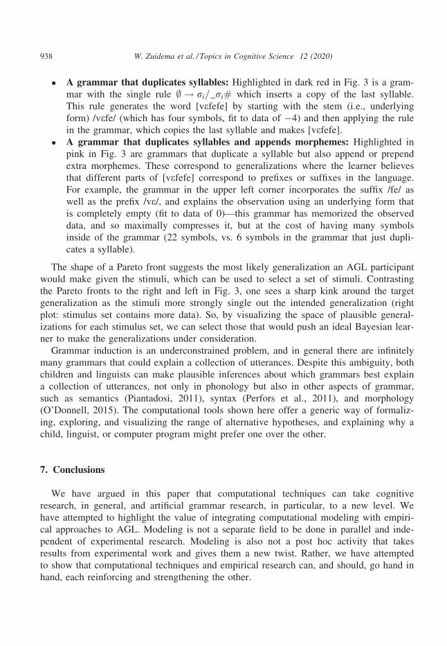
• A grammar that duplicates syllables: Highlighted in dark red in Fig. 3 is a gram-

mar with the single rule ; ! ri= ri# which inserts a copy of the last syllable.

This rule generates the word [vefefe] by starting with the stem (i.e., underlying

form) /vefe/ (which has four symbols, fit to data of �4) and then applying the rule

in the grammar, which copies the last syllable and makes [vefefe].

• A grammar that duplicates syllables and appends morphemes: Highlighted in

pink in Fig. 3 are grammars that duplicate a syllable but also append or prepend

extra morphemes. These correspond to generalizations where the learner believes

that different parts of [vefefe] correspond to prefixes or suffixes in the language.

For example, the grammar in the upper left corner incorporates the suffix /fe/ as

well as the prefix /ve/, and explains the observation using an underlying form that

is completely empty (fit to data of 0)—this grammar has memorized the observed

data, and so maximally compresses it, but at the cost of having many symbols

inside of the grammar (22 symbols, vs. 6 symbols in the grammar that just dupli-

cates a syllable).

The shape of a Pareto front suggests the most likely generalization an AGL participant

would make given the stimuli, which can be used to select a set of stimuli. Contrasting

the Pareto fronts to the right and left in Fig. 3, one sees a sharp kink around the target

generalization as the stimuli more strongly single out the intended generalization (right

plot: stimulus set contains more data). So, by visualizing the space of plausible general-

izations for each stimulus set, we can select those that would push an ideal Bayesian lear-

ner to make the generalizations under consideration.

Grammar induction is an underconstrained problem, and in general there are infinitely

many grammars that could explain a collection of utterances. Despite this ambiguity, both

children and linguists can make plausible inferences about which grammars best explain

a collection of utterances, not only in phonology but also in other aspects of grammar,

such as semantics (Piantadosi, 2011), syntax (Perfors et al., 2011), and morphology

(O’Donnell, 2015). The computational tools shown here offer a generic way of formaliz-

ing, exploring, and visualizing the range of alternative hypotheses, and explaining why a

child, linguist, or computer program might prefer one over the other.

7. Conclusions

We have argued in this paper that computational techniques can take cognitive

research, in general, and artificial grammar research, in particular, to a new level. We

have attempted to highlight the value of integrating computational modeling with empiri-

cal approaches to AGL. Modeling is not a separate field to be done in parallel and inde-

pendent of experimental research. Modeling is also not a post hoc activity that takes

results from experimental work and gives them a new twist. Rather, we have attempted

to show that computational techniques and empirical research can, and should, go hand in

hand, each reinforcing and strengthening the other.


In particular, we have discussed how computational modeling techniques can be used

for clarifying theories: the process of formalization forces us to specify details of our the-

ories that would otherwise have remained vague, and the formalized (and implemented)

models allow us to potentially derive unexpected consequences from our assumptions—as

discussed in Section 2, using the example of the phenomenon of “word segmentation” in

artificial language learning experiments.

In addition, we discussed the role models play in suggesting new experiments: We can

use computational models to derive new, testable predictions (Sections 2 and 4), to gener-

ate stimuli for experiments (Sections 3 and 4), and even to generate new, testable

hypotheses (Section 6).

Finally, we pointed to the useful function of models to give us novel insights about

experimental data: by providing visualization techniques that show structure not visible

with standard techniques (Section 4), and by allowing us to test the goodness of fit of a

range of alternative models to the data (Section 5).

Acknowledgments

W.Z. is funded by the Gravitation Program “Language in Interaction” of the Nether-

lands Organization for Scientific Research (Gravitation Grant 024.001.006). K.E. is

funded by a NSF GRFP grant. T.S. is also funded by a NSF GRFP grant (2017216247).

The work reported by R.M.F was funded in part by a grant (ORA-10-056) from the

French National Research Agency (ANR) and the ESRC of the United Kingdom. We

thank NVIDIA for donating a GPU to T.Q.G. in this work.

Note

1. In this case, the contribution of the hidden unit activations, which constitute the

network’s internal representation of the two items on input at time t, to RHSt+1 will

be large, because tanh(Dt) will be close to zero; conversely, if Dt is large, meaning

that the items on input have not been seen together often, the hidden layer’s contri-

bution to LHS at time t + 1 will be relatively small because tanh(Dt) will be close

to 1, meaning that 1 � tanh(Dt) will be close to zero).

References

Alhama, R. G., Scha, R., & Zuidema, W. (2015). How should we evaluate models of segmentation in

artificial language learning? In N. A. Taatgen, M. K. van Vugt, J. P. Borst & K. Mehlhorn (Eds.),

Proceedings of 13th international conference on cognitive modeling (pp. 172–173). Groningen, The

netherlands: University of Groningen


Alhama, R. G., & Zuidema, W. (2017). Segmentation as Retention and Recognition: The R&R model. In G.

Gunzelmann, A. Howes, T. Tenbrink, & E. Davelaar (Eds.), Proceedings of the 39th Annual Conferenceof the Cognitive Science Society (pp. 1531–1536). Austin, TX: Cognitive Science Society

Alhama, R. G., & Zuidema, W. (2019). A review of computational models of basic rule learning: The

neural-symbolic debate and beyond. Psychonomic Bulletin & Review, 26(4), 1174–1194.Beckers, G. J. L., Berwick, R. C., Okanoya, K., & Bolhuis, J. J. (2016). What do animals learn in artificial

grammar studies? Neuroscience & Biobehavioral Reviews, 81, 238–246.Chomsky, N., & Halle, M. (1968). The sound pattern of English. New York: Harper & Row.

Claeskens, G. (2016). Statistical model choice. Annual Review of Statistics and Its Application, 3, 233–256.

Cleeremans, A., & French, R. M. (1996). From chicken squawking to cognition: Levels of description and

the computational approach in psychology. Psychologica Belgica, 36, 5–29.Culbertson, J., Smolensky, P., & Wilson, C. (2013). Cognitive biases, linguistic universals, and constraint-

based grammar learning. Topics in Cognitive Science, 5(3), 392–424.Ellis, K., Solar-Lezama, A., & Tenenbaum, J. (2015). In C. Cortes, N. D. Lawrence, D. D. Lee , M.

Sugiyama, & R. Garnett (Eds.), Advances in neural information processing systems 28: AnnualConference on Neural Information Processing Systems 2015, December 7-12, 2015 (pp. 973–981).Montreal, Quebec, Canada.

Elman, J. L. (1990). Finding structure in time. Cognitive Science, 14(2), 179–211.Forster, K. I. (2000). The potential for experimenter bias effects in word recognition experiments. Memory &

Cognition, 28(7), 1109–1115.Frank, M. C., Goldwater, S., Griffiths, T. L., & Tenenbaum, J. B. (2010). Modeling human performance in

statistical word segmentation. Cognition, 117(2), 107–125.French, R. M., Addyman, C., & Mareschal, D. (2011). TRACX: A recognition-based connectionist

framework for sequence segmentation and chunk extraction. Psychological Review, 118(4), 614–636.French, R. M., & Cottrell, G. (2014). TRACX 2.0: A memory-based, biologically-plausible model of

sequence segmentation and chunk extraction. In P. Bello,M. Guarini, M. McShane, & B. Scassellati

(Eds.), Proceedings of the 36th Annual Conference of the Cognitive Science Society (pp. 2216–2221).Austin, TX: Cognitive Science Society.

Gagliardi, A., Feldman, N. H., & Lidz, J. (2017). Modeling statistical insensitivity: Sources of suboptimal

behavior. Cognitive Science, 41(1), 188–217.Gerken, L. (2010). Infants use rational decision criteria for choosing among models of their input. Cognition,

115(2), 362–366.Hedley, R. W. (2016). Complexity, predictability and time homogeneity of syntax in the songs of cassin’s

vireo (vireo cassinii). PLoS ONE, 11(4), e0150822.Kemp, C., Perfors, A., & Tenenbaum, J. B. (2007). Learning overhypotheses with hierarchical bayesian

models. Developmental Science, 10(3), 307–321.Kirby, S., Tamariz, M., Cornish, H., & Smith, K. (2015). Compression and communication in the cultural

evolution of linguistic structure. Cognition, 141, 87–102.Kurumada, C., Meylan, S. C., & Frank, M. C. (2013). Zipfian frequency distributions facilitate word

segmentation in context. Cognition, 127(3), 439–453.Marcus, G. F., Vijayan, S., Rao, S. B., & Vishton, P. M. (1999). Rule learning by seven-month-old infants.

Science, 283(5398), 77–80.Mareschal, D., & French, R. M. (2017). TRACX2: A connectionist autoencoder using graded chunks to

model infant visual statistical learning. Philosophical Transactions of the Royal Society B: BiologicalSciences, 372(1711), 20160057.

Mattson, C. A., & Messac, A. (2005). Pareto frontier based concept selection under uncertainty, with

visualization. Optimization and Engineering, 6(1), 85–115.McInnes, L., & Healy, J. (2017). Accelerated hierarchical density based clustering. In Data mining

workshops (ICDMW), 2017 IEEE international conference on (pp. 33–42). New Orleans, LA: IEEE.


O’Donnell, T. J. (2015). Productivity and reuse in language: A theory of linguistic computation and storage.Cambridge, MA: The MIT Press.

Onnis, L., Monaghan, P., Richmond, K., & Chater, N. (2005). Phonology impacts segmentation in online

speech processing. Journal of Memory and Language, 53(2), 225–237.Pearl, L., Goldwater, S., & Steyvers, M. (2010). Online learning mechanisms for bayesian models of word

segmentation. Research on Language and Computation, 8(2–3), 107–132.Pelucchi, B., Hay, J. F., & Saffran, J. R. (2009). Learning in reverse: Eight-month-old infants track backward

transitional probabilities. Cognition, 113(2), 244–247.Pe~na, M., Bonatti, L. L., Nespor, M., & Mehler, J. (2002). Signal-driven computations in speech processing.

Science, 298(5593), 604–607.Perfors, A., Tenenbaum, J. B., & Regier, T. (2011). The learnability of abstract syntactic principles.

Cognition, 118(3), 306–338.Perruchet, P., & Desaulty, S. (2008). A role for backward transitional probabilities in word segmentation?

Memory & Cognition, 36(7), 1299–1305.Perruchet, P., Peereman, R., & Tyler, M. D. (2006). Do we need algebraic-like computations? A reply to

Bonatti, Pe~na, Nespor, and Mehler (2006). Journal of Experimental Psychology: General, 135(3), 461.Piantadosi, S. T. (2011). Learning and the language of thought. Unpublished doctoral dissertation,

Massachusetts Institute of Technology.

Ravignani, A., Westphal-Fitch, G., Aust, U., Schlumpp, M. M., & Fitch, W. T. (2015). More than one way to

see it: Individual heuristics in avian visual computation. Cognition, 143, 13–24.Rochester, N., Holland, J., Haibt, L., & Duda, W. (1956). Tests on a cell assembly theory of the action of

the brain, using a large digital computer. IRE Transactions on Information Theory, 2(3), 80–93.Seidenberg, M. S., MacDonald, M. C., & Saffran, J. R. (2002). Does grammar start where statistics stop?

Science, 298(5593), 553–554.Slone, L., & Johnson, S. P. (2015). Statistical and chunking processes in adults visual sequence learning. In

SRCD biannual conference. Philadelphia, PA.

Van Heijningen, C. A. A., De Visser, J., Zuidema, W., & Ten Cate, C. (2009). Simple rules can explain

discrimination of putative recursive syntactic structures by a songbird species. Proceedings of the NationalAcademy of Sciences, 106(48), 20538–20543.

Wonnacott, E. (2011). Balancing generalization and lexical conservatism: An artificial language study with

child learners. Journal of Memory and Language, 65(1), 1–14.


Documents

Five Ways in Which Computational Modeling Can Help Advance