Embed Size (px)
Citation preview
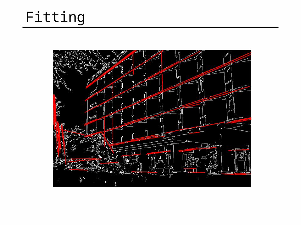
Fitting
Fitting
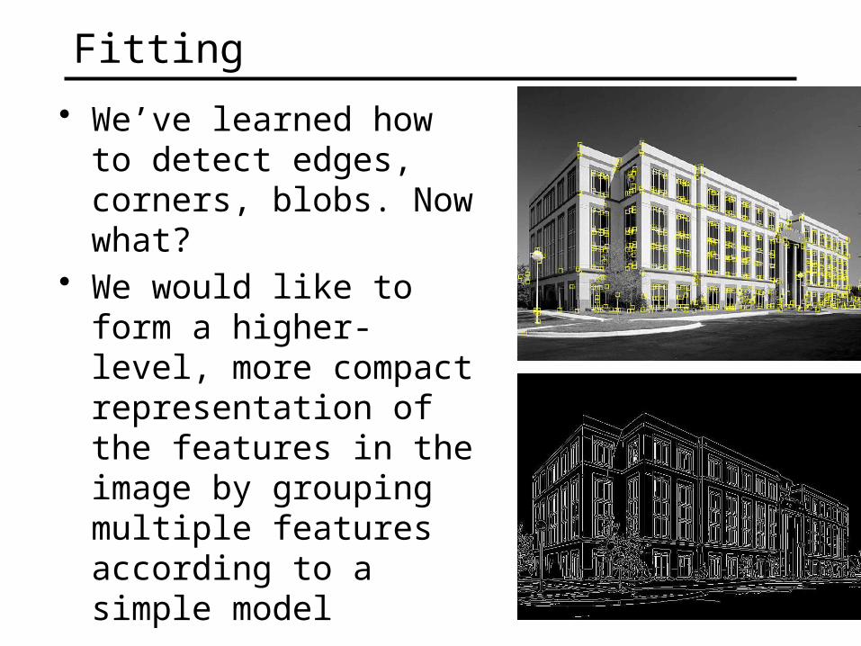
• We’ve learned how to detect edges, corners, blobs. Now what?
• We would like to form a higher-level, more compact representation of the features in the image by grouping multiple features according to a simple model
Source: K. Grauman
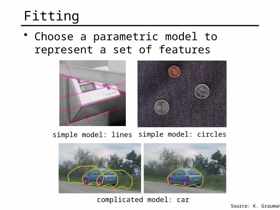
Fitting• Choose a parametric model to represent a
set of features
simple model: lines simple model: circles
complicated model: car
Fitting: Issues
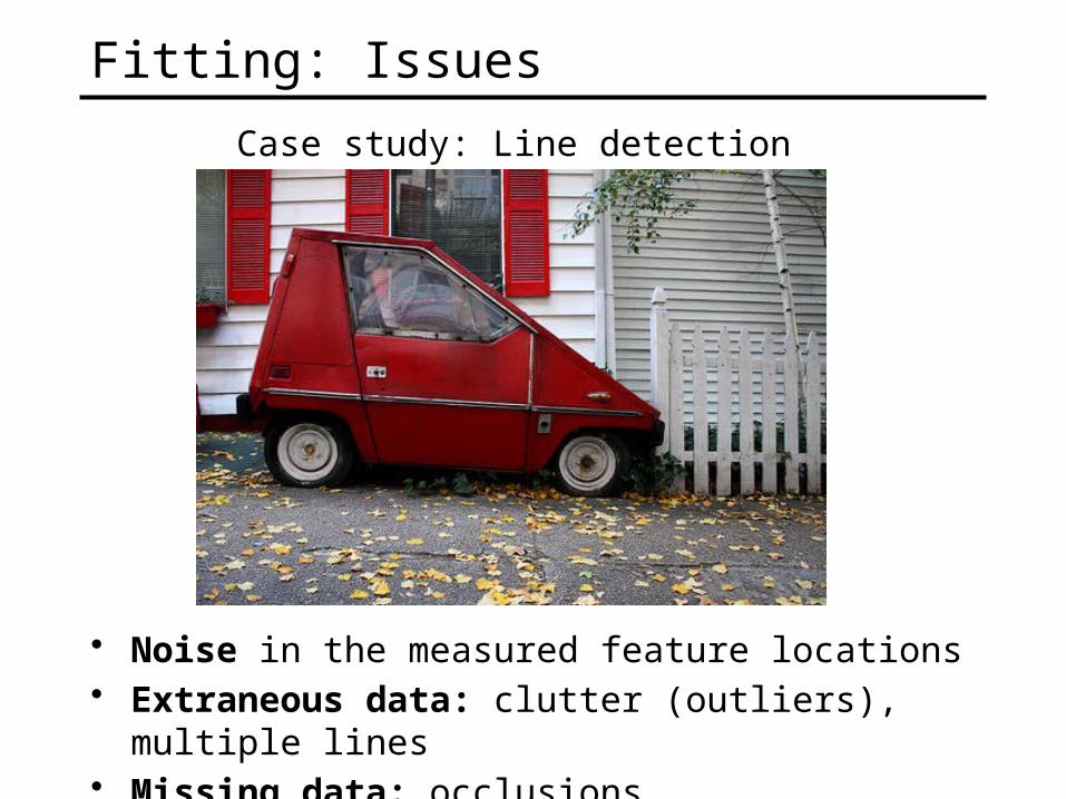
• Noise in the measured feature locations• Extraneous data: clutter (outliers), multiple lines• Missing data: occlusions
Case study: Line detection
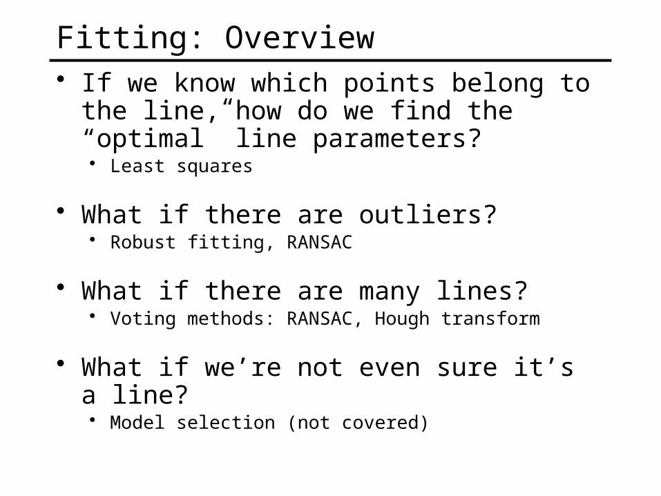
Fitting: Overview• If we know which points belong to the line,
how do we find the “optimal” line parameters?• Least squares
• What if there are outliers?• Robust fitting, RANSAC
• What if there are many lines?• Voting methods: RANSAC, Hough transform
• What if we’re not even sure it’s a line?• Model selection (not covered)
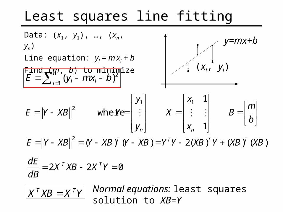
Least squares line fittingData: (x1, y1), …, (xn, yn)
Line equation: yi = m xi + b
Find (m, b) to minimize
022 YXXBXdB
dE TT
b
mB
x
x
X
y
y
YXBYE
nn 1
1
where11
2
Normal equations: least squares solution to XB=Y
n
i ii bxmyE1
2)((xi, yi)
y=mx+b
YXXBX TT
)()()(2)()(2
XBXBYXBYYXBYXBYXBYE TTTT
Problem with “vertical” least squares• Not rotation-invariant• Fails completely for vertical lines
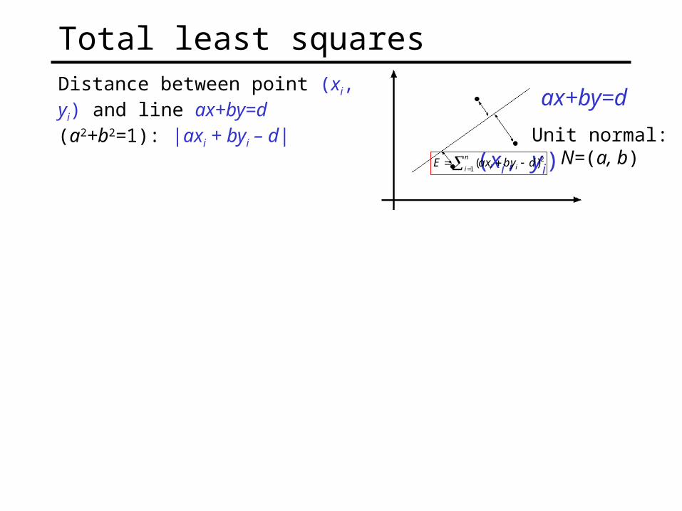
Total least squaresDistance between point (xi, yi) and line ax+by=d (a2+b2=1): |axi + byi – d|
n
i ii dybxaE1
2)( (xi, yi)
ax+by=d
Unit normal: N=(a, b)
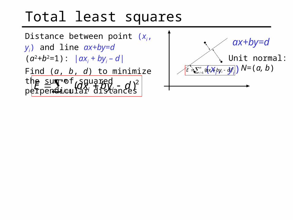
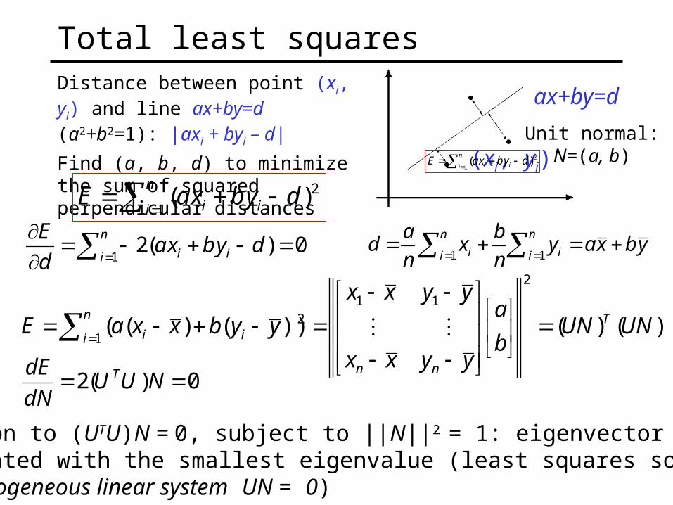
Total least squaresDistance between point (xi, yi) and line ax+by=d (a2+b2=1): |axi + byi – d|
Find (a, b, d) to minimize the sum of squared perpendicular distances
n
i ii dybxaE1
2)( (xi, yi)
ax+by=d
n
i ii dybxaE1
2)(
Unit normal: N=(a, b)
Total least squaresDistance between point (xi, yi) and line ax+by=d (a2+b2=1): |axi + byi – d|
Find (a, b, d) to minimize the sum of squared perpendicular distances
n
i ii dybxaE1
2)( (xi, yi)
ax+by=d
n
i ii dybxaE1
2)(
Unit normal: N=(a, b)
0)(21
n
i ii dybxad
Eybxay
n
bx
n
ad
n
i i
n
i i 11
)()())()((
2
11
1
2 UNUNb
a
yyxx
yyxx
yybxxaE T
nn
n
i ii
0)(2 NUUdN
dE T
Solution to (UTU)N = 0, subject to ||N||2 = 1: eigenvector of UTUassociated with the smallest eigenvalue (least squares solution to homogeneous linear system UN = 0)
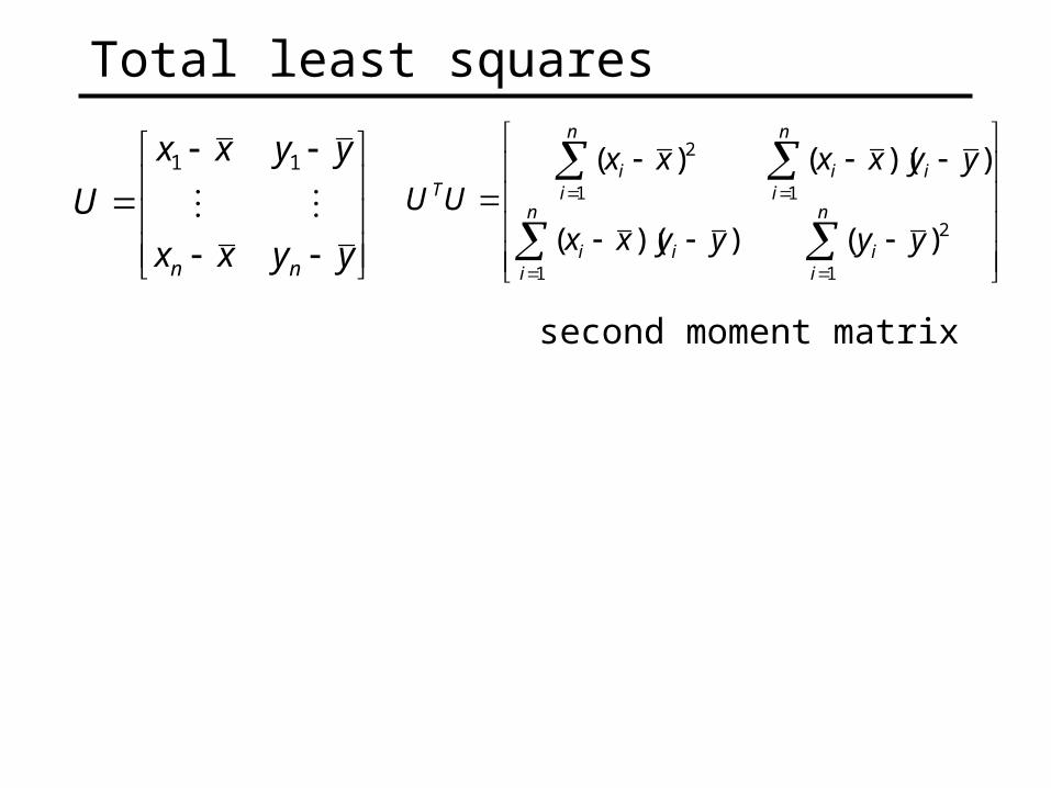
Total least squares
yyxx
yyxx
U
nn
11
n
ii
n
iii
n
iii
n
ii
T
yyyyxx
yyxxxxUU
1
2
1
11
2
)())((
))(()(
second moment matrix
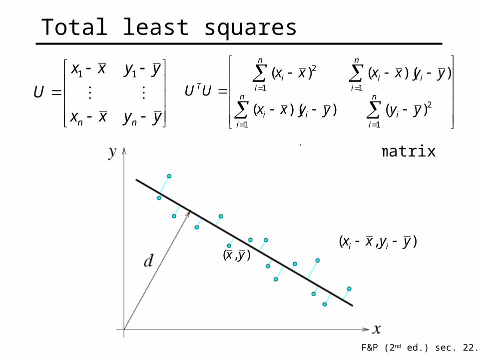
Total least squares
yyxx
yyxx
U
nn
11
n
ii
n
iii
n
iii
n
ii
T
yyyyxx
yyxxxxUU
1
2
1
11
2
)())((
))(()(
),( yx
N = (a, b)
second moment matrix
),( yyxx ii
F&P (2nd ed.) sec. 22.1
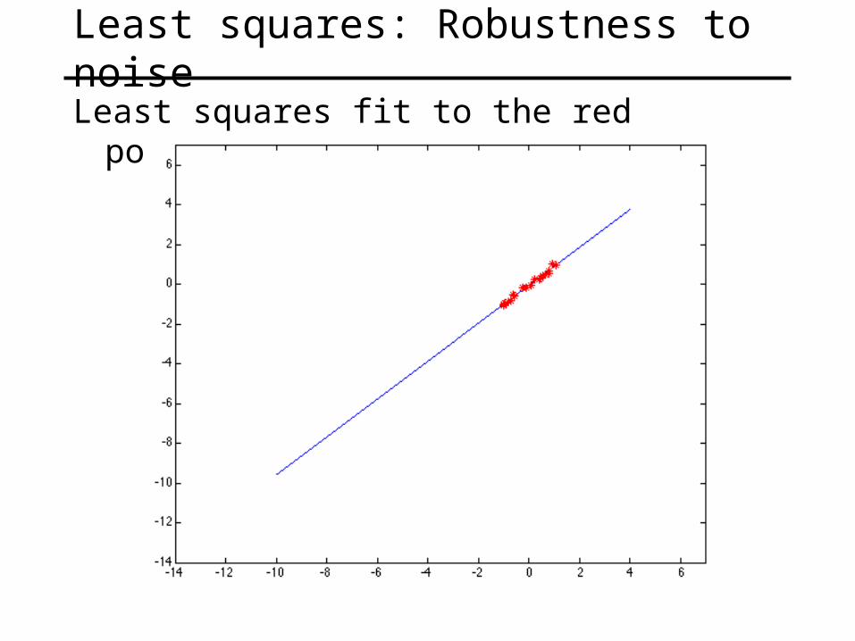
Least squares: Robustness to noise
Least squares fit to the red points:
Least squares: Robustness to noise
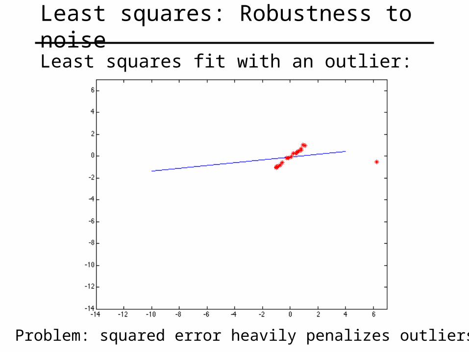
Least squares fit with an outlier:
Problem: squared error heavily penalizes outliers
Robust estimators
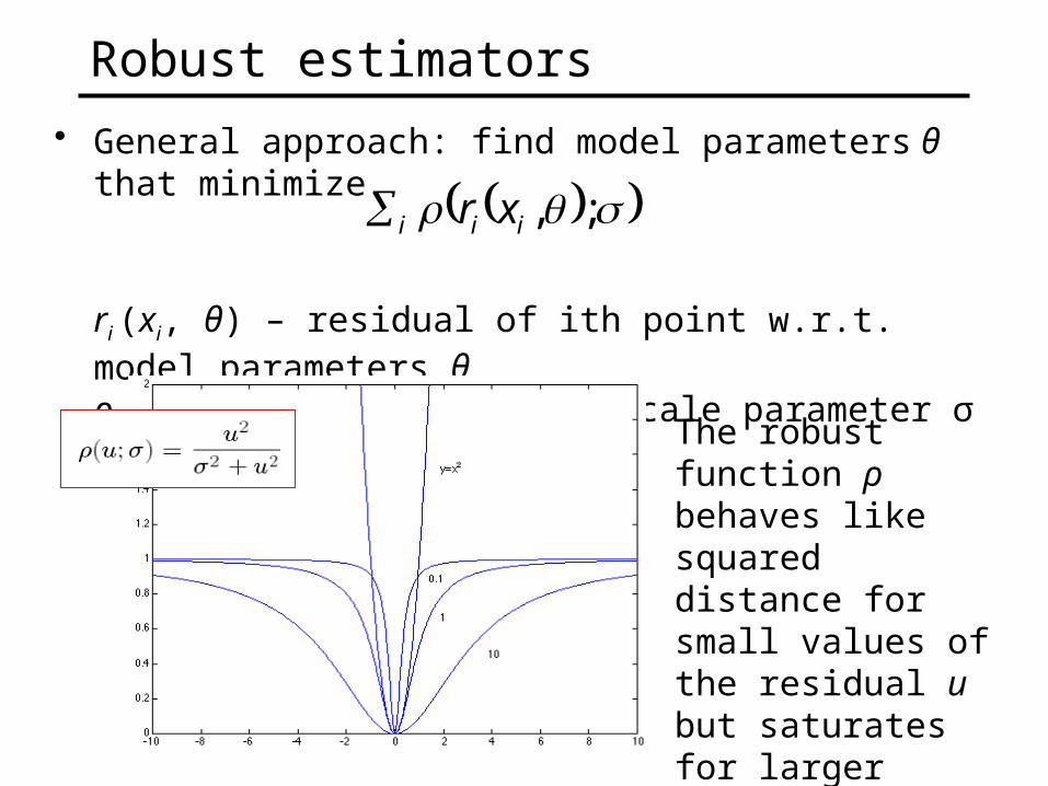
• General approach: find model parameters θ that minimize
ri (xi, θ) – residual of ith point w.r.t. model parameters θρ – robust function with scale parameter σ
;,iii xr
The robust function ρ behaves like squared distance for small values of the residual u but saturates for larger values of u
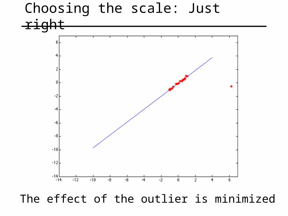
Choosing the scale: Just right
The effect of the outlier is minimized
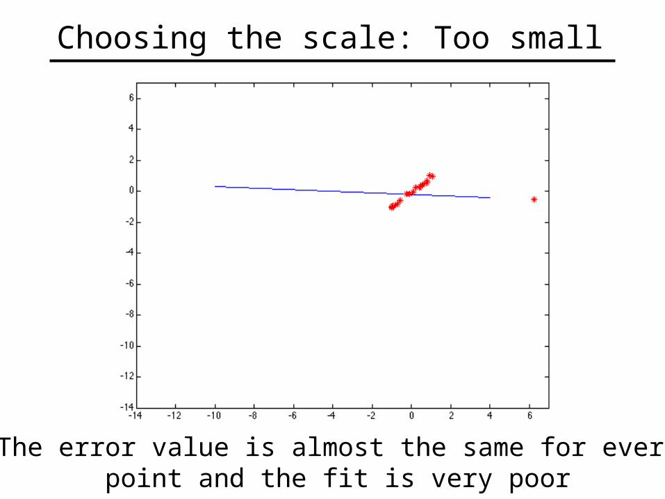
The error value is almost the same for everypoint and the fit is very poor
Choosing the scale: Too small
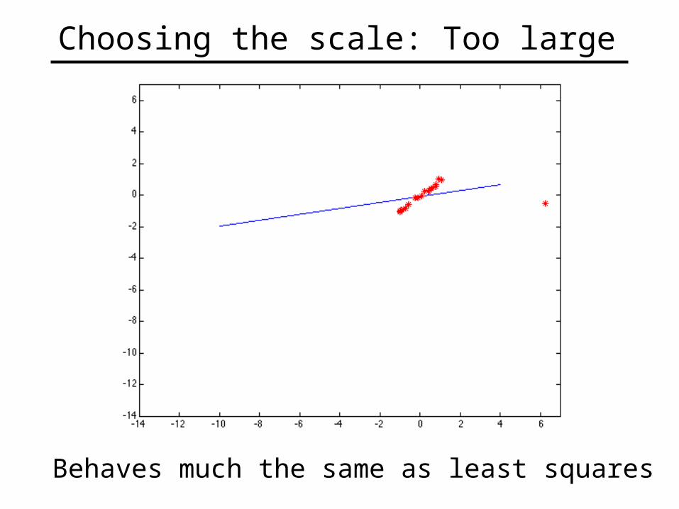
Choosing the scale: Too large
Behaves much the same as least squares
Robust estimation: Details• Robust fitting is a nonlinear optimization
problem that must be solved iteratively• Least squares solution can be used for
initialization• Scale of robust function should be chosen
adaptively based on median residual
RANSAC• Robust fitting can deal with a few outliers –
what if we have very many?• Random sample consensus (RANSAC):
Very general framework for model fitting in the presence of outliers
• Outline• Choose a small subset of points uniformly at random• Fit a model to that subset• Find all remaining points that are “close” to the model and
reject the rest as outliers• Do this many times and choose the best model
M. A. Fischler, R. C. Bolles. Random Sample Consensus: A Paradigm for Model Fitting with Applications to Image Analysis and Automated Cartography. Comm. of the ACM, Vol 24, pp 381-395, 1981.
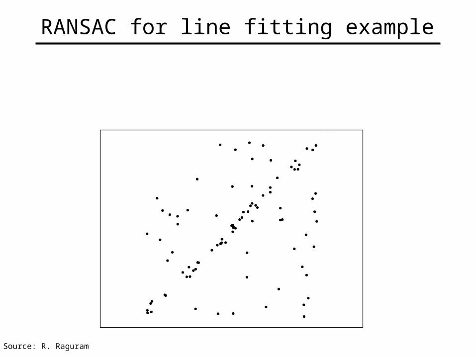
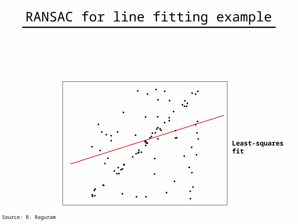
RANSAC for line fitting example
Source: R. Raguram
RANSAC for line fitting example
Least-squares fit
Source: R. Raguram

RANSAC for line fitting example
1. Randomly select minimal subset of points
Source: R. Raguram
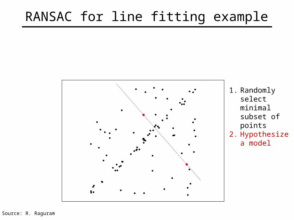
RANSAC for line fitting example
1. Randomly select minimal subset of points
2. Hypothesize a model
Source: R. Raguram
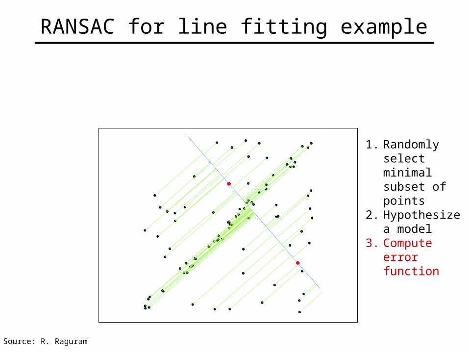
RANSAC for line fitting example
1. Randomly select minimal subset of points
2. Hypothesize a model
3. Compute error function
Source: R. Raguram
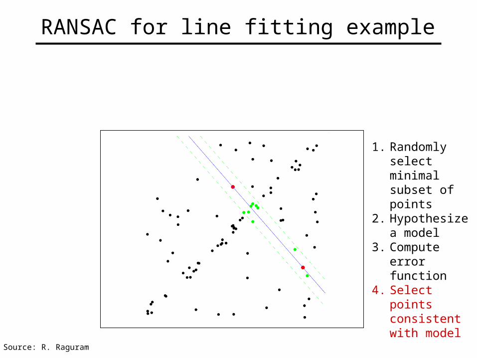
RANSAC for line fitting example
1. Randomly select minimal subset of points
2. Hypothesize a model
3. Compute error function
4. Select points consistent with model
Source: R. Raguram
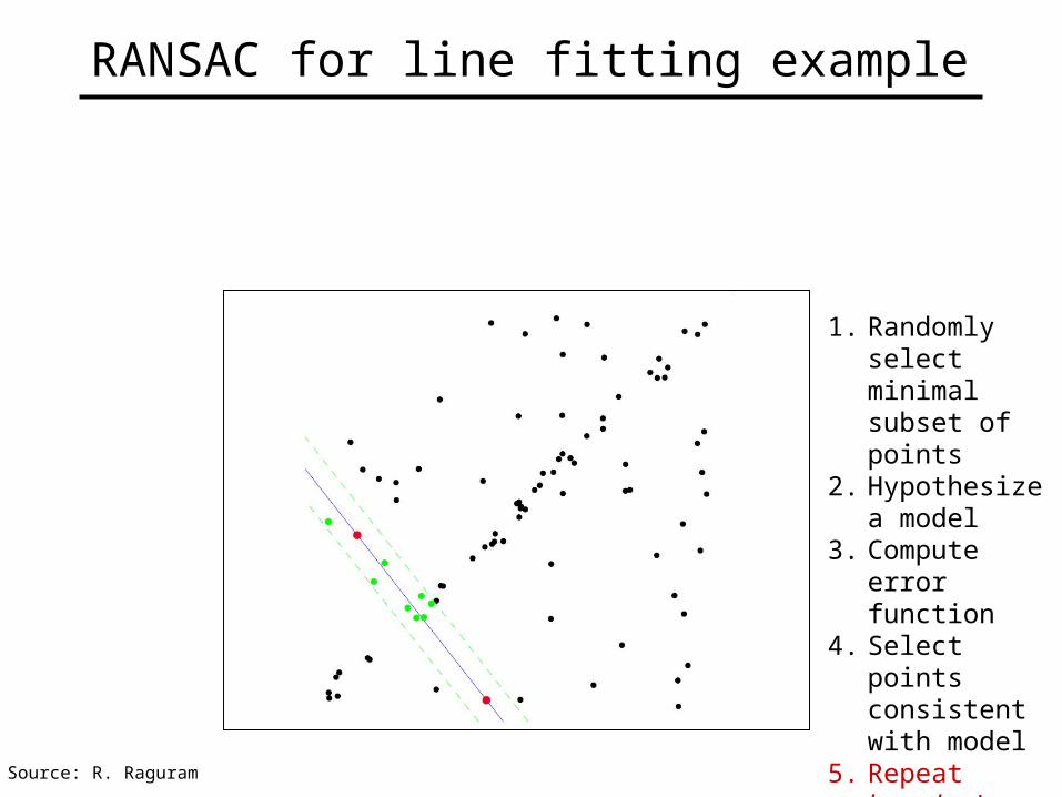
RANSAC for line fitting example
1. Randomly select minimal subset of points
2. Hypothesize a model
3. Compute error function
4. Select points consistent with model
5. Repeat hypothesize-and-verify loop
Source: R. Raguram
30
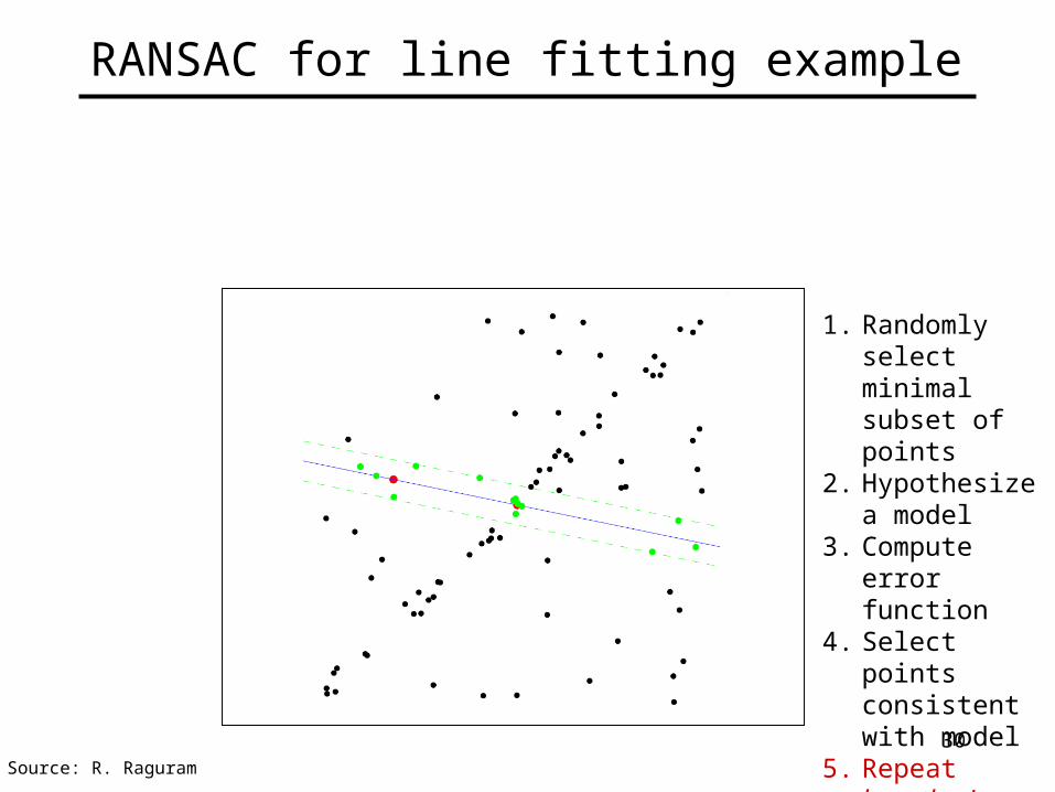
RANSAC for line fitting example
1. Randomly select minimal subset of points
2. Hypothesize a model
3. Compute error function
4. Select points consistent with model
5. Repeat hypothesize-and-verify loop
Source: R. Raguram
31
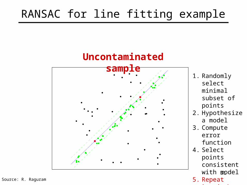
RANSAC for line fitting example
1. Randomly select minimal subset of points
2. Hypothesize a model
3. Compute error function
4. Select points consistent with model
5. Repeat hypothesize-and-verify loop
Uncontaminated sample
Source: R. Raguram
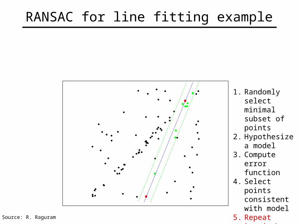
RANSAC for line fitting example
1. Randomly select minimal subset of points
2. Hypothesize a model
3. Compute error function
4. Select points consistent with model
5. Repeat hypothesize-and-verify loop
Source: R. Raguram
RANSAC for line fitting
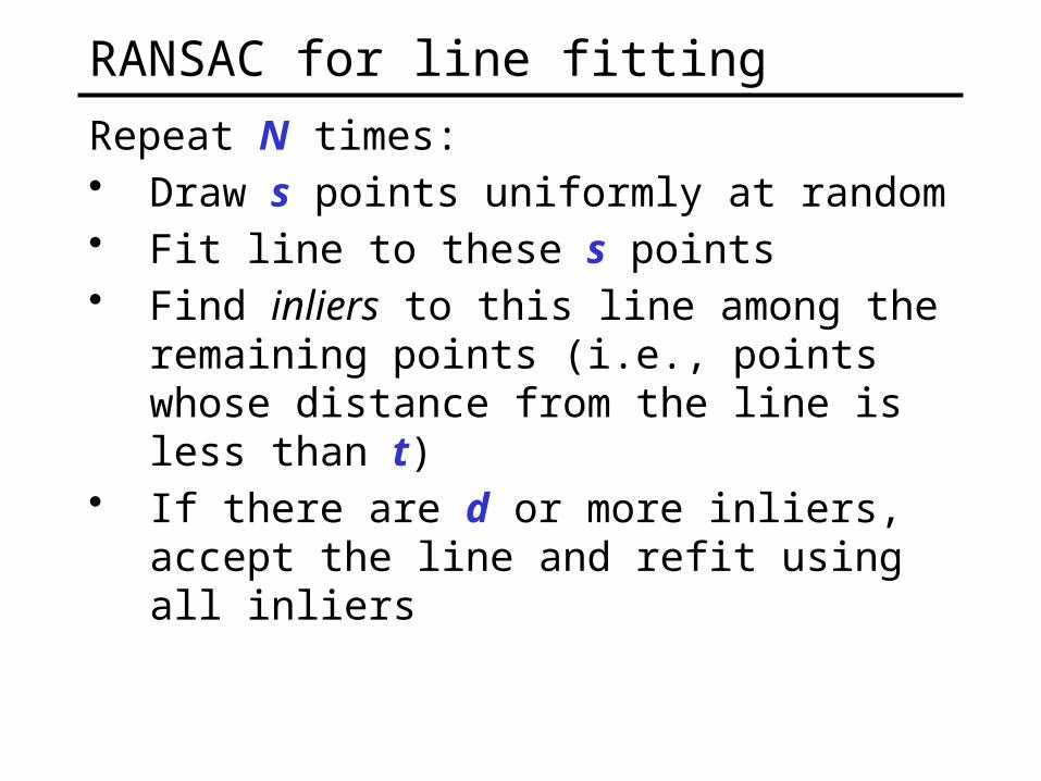
Repeat N times:• Draw s points uniformly at random• Fit line to these s points• Find inliers to this line among the remaining
points (i.e., points whose distance from the line is less than t)
• If there are d or more inliers, accept the line and refit using all inliers
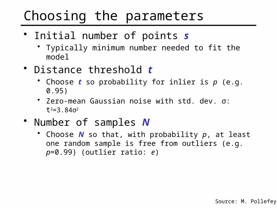
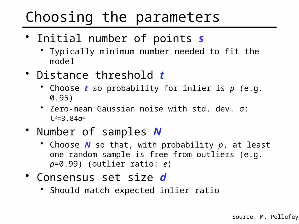
Choosing the parameters• Initial number of points s
• Typically minimum number needed to fit the model
• Distance threshold t• Choose t so probability for inlier is p (e.g. 0.95) • Zero-mean Gaussian noise with std. dev. σ: t2=3.84σ2
• Number of samples N• Choose N so that, with probability p, at least one random
sample is free from outliers (e.g. p=0.99) (outlier ratio: e)
Source: M. Pollefeys
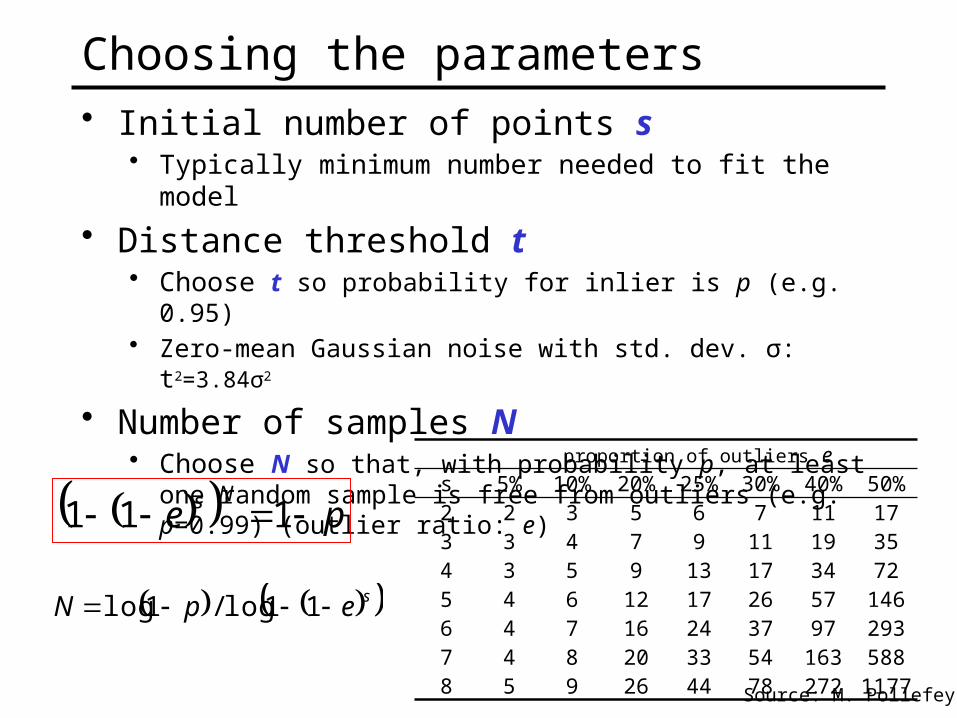
Choosing the parameters
sepN 11log/1log
peNs 111
proportion of outliers es 5% 10% 20% 25% 30% 40% 50%2 2 3 5 6 7 11 173 3 4 7 9 11 19 354 3 5 9 13 17 34 725 4 6 12 17 26 57 1466 4 7 16 24 37 97 2937 4 8 20 33 54 163 5888 5 9 26 44 78 272 1177
Source: M. Pollefeys
• Initial number of points s• Typically minimum number needed to fit the model
• Distance threshold t• Choose t so probability for inlier is p (e.g. 0.95) • Zero-mean Gaussian noise with std. dev. σ: t2=3.84σ2
• Number of samples N• Choose N so that, with probability p, at least one random
sample is free from outliers (e.g. p=0.99) (outlier ratio: e)
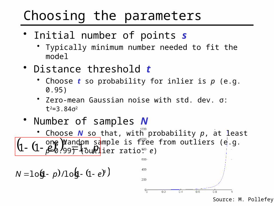
Choosing the parameters
peNs 111
Source: M. Pollefeys
sepN 11log/1log
• Initial number of points s• Typically minimum number needed to fit the model
• Distance threshold t• Choose t so probability for inlier is p (e.g. 0.95) • Zero-mean Gaussian noise with std. dev. σ: t2=3.84σ2
• Number of samples N• Choose N so that, with probability p, at least one random
sample is free from outliers (e.g. p=0.99) (outlier ratio: e)
Choosing the parameters• Initial number of points s
• Typically minimum number needed to fit the model
• Distance threshold t• Choose t so probability for inlier is p (e.g. 0.95) • Zero-mean Gaussian noise with std. dev. σ: t2=3.84σ2
• Number of samples N• Choose N so that, with probability p, at least one random
sample is free from outliers (e.g. p=0.99) (outlier ratio: e)
• Consensus set size d• Should match expected inlier ratio
Source: M. Pollefeys
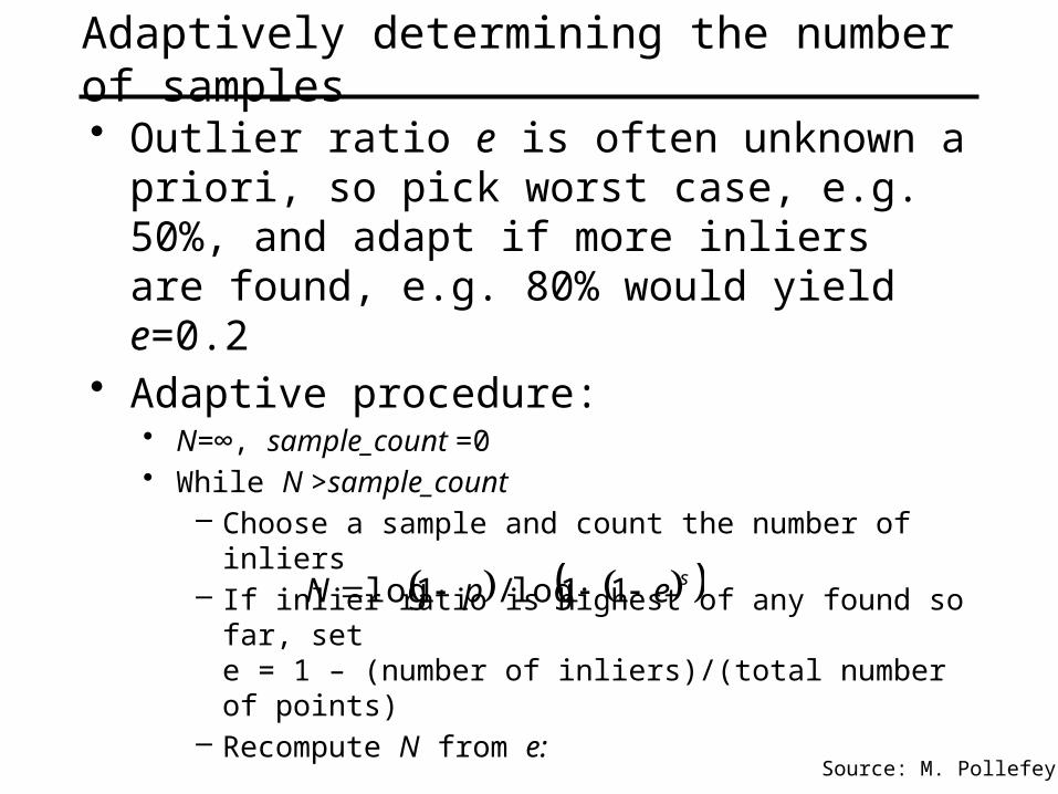
Adaptively determining the number of samples
• Outlier ratio e is often unknown a priori, so pick worst case, e.g. 50%, and adapt if more inliers are found, e.g. 80% would yield e=0.2
• Adaptive procedure:• N=∞, sample_count =0• While N >sample_count
– Choose a sample and count the number of inliers– If inlier ratio is highest of any found so far, set
e = 1 – (number of inliers)/(total number of points)– Recompute N from e:
– Increment the sample_count by 1
sepN 11log/1log
Source: M. Pollefeys
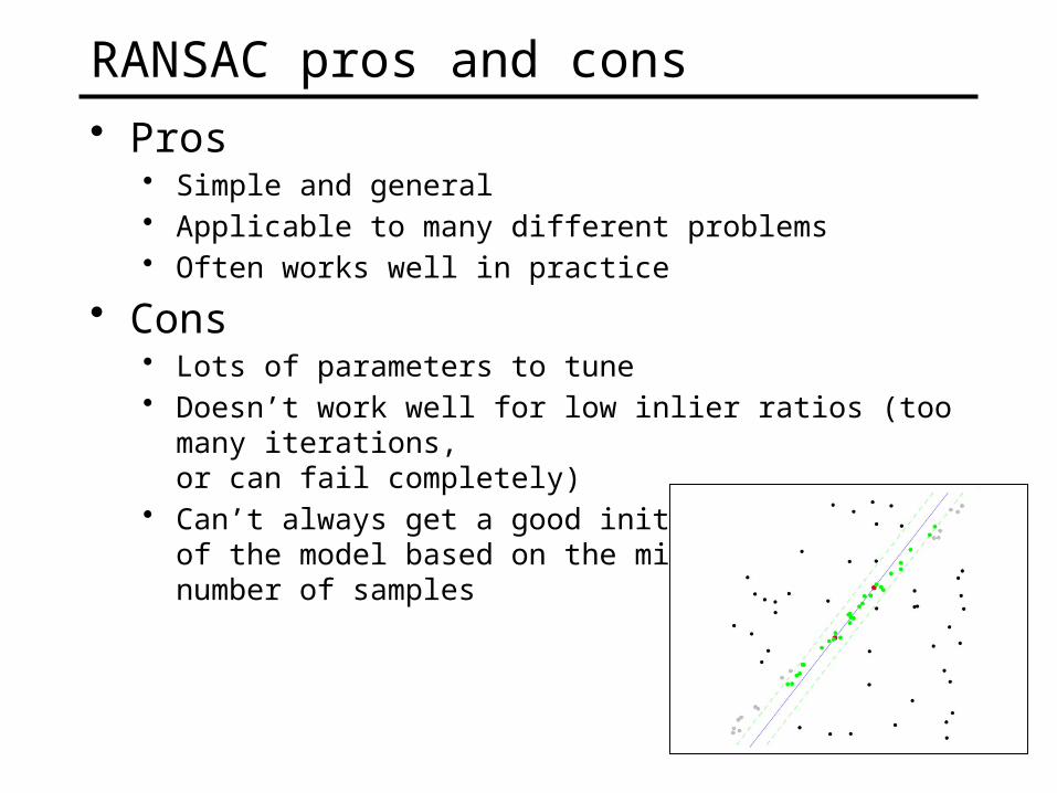
RANSAC pros and cons• Pros
• Simple and general• Applicable to many different problems• Often works well in practice
• Cons• Lots of parameters to tune• Doesn’t work well for low inlier ratios (too many iterations,
or can fail completely)• Can’t always get a good initialization
of the model based on the minimum number of samples