Embed Size (px)
Citation preview

Fitting Primitive Shapes to Point Clouds for Robotic Grasping
S E R G I O G A R C Í A
Master of Science Thesis Stockholm, Sweden 2009
Fitting Primitive Shapes to Point Clouds for Robotic Grasping
S E R G I O G A R C Í A
Master’s Thesis in Computer Science (30 ECTS credits) at the School of Electrical Engineering Royal Institute of Technology year 2009 Supervisor at CSC was Danica Kragic Examiner was Danica Kragic TRITA-CSC-E 2009:131 ISRN-KTH/CSC/E--09/131--SE ISSN-1653-5715 Royal Institute of Technology School of Computer Science and Communication KTH CSC SE-100 44 Stockholm, Sweden URL: www.csc.kth.se
iii
Abstract
Due to the growth of service robots in the last few years, made it possiblethat robots can carry out human tasks. Houseworks that for humans wouldseem as common and simple as grasping, moving and interacting with objects,are a challenge both mechanically and computationally in robotics.
Therefore, considering the process of grasping objects by robotic machines,this thesis introduces an algorithm that makes the identification of complexobjects easier by using a set of geometric primitive shapes already known tothe robot. Thus, taking as input the point clouds which define the 3D objectsonce they have been scanned, an algorithm based on the iterative methodRANSAC has been developed. The proposed algorithm is able to fit a set ofprimitive shapes to an incomplete and noisy point cloud.
By splitting input point clouds into smaller sets, the suggested algorithmattempts to find the primitive shape that best fits each of these divisions inorder to simplify the 3D objects. Consequently, a robot will be able to recognizeunknown objects without the need of having previously stored objects in itsdatabase. The huge amount of possible grasps that can be applied to an objectis therefore reduced to just a few based on the division into primitive shapes.
Additionally, this thesis explains how each of the estimation algorithmshave been designed, as well as evaluates the performance of these under differentnoise conditions.

Acknowledgements
First of all, I would like to express my gratitude to the CVAP department atKTH for allowing me to develop this project with them. Thanks to JeannetteBohg for her patience, dedication and support throughout the developmentof the thesis. Thanks to Javier Romero González for helping me to find thisthesis and spend his time every time that I asked him for any problem. Thanksalso to Kai Hübner, Carl Barck-Holst, Albert Pla and Oscar Rubio Martin forcollaborating in my thesis with their ideas and knowledges.
I would also like to thank to Jorge Sánchez de Nova, who has been myworkmate during this thesis, for his indispensable help, advice and suggestions.
My infinite thankfulness to my father and mother that made feasible mystudies in a foreign country. My gratitude also to my sister for helping me withthe thesis report. I cannot forget to my girlfriend for all her support and formaking possible our relationship despite the distance.
Finally, I am also very thankful to all the friends that I have met duringmy stay in Sweden, with whom I have spent great times and because withoutthem this experience had not been the same.
v

Acronyms
PACO-PLUS Perception, Action and COgnition
RANSAC RANdom SAmple Consensus
MATLAB MATrix LABoratory
MSS Minimal Sample Set
CS Consensus Set
RN Random Noise
RNIM Random Noise with Incomplete Model
SN Surface Noise
SNIM Surface Noise with Incomplete Model
MSAC M-estimator SAmple and Consensus
MLESAC Maximum Likelihood Estimation SAmple Consensus
PROSAC PROgressive SAmple Consensus
MVBB Minimum Volume Bounding Box
ICP Iterative Closest Point
MEE Mean Estimated Error
CVAP Computer Vision and Active Perception laboratory
PSDA Primitive Shape Decomposition Algorithm
vii

Contents
Contents viii
1 Introduction 11.1 PACO-PLUS Project . . . . . . . . . . . . . . . . . . . . . . . . . . . 11.2 Primitive Shapes . . . . . . . . . . . . . . . . . . . . . . . . . . . . . 21.3 Simplification of the Object Database . . . . . . . . . . . . . . . . . 2
2 Related Work 52.1 Related Articles . . . . . . . . . . . . . . . . . . . . . . . . . . . . . . 52.2 The BoxDecomposition Algorithm . . . . . . . . . . . . . . . . . . . 62.3 The RANSAC Algorithm . . . . . . . . . . . . . . . . . . . . . . . . 7
2.3.1 RANSAC nomenclature . . . . . . . . . . . . . . . . . . . . . 92.3.2 RANSAC variations . . . . . . . . . . . . . . . . . . . . . . . 9
3 Fitting Primitive Shapes to Point Clouds 113.1 RANSAC in MatLab . . . . . . . . . . . . . . . . . . . . . . . . . . . 11
3.1.1 Main loop phase . . . . . . . . . . . . . . . . . . . . . . . . . 123.1.2 Primitive shape estimation function . . . . . . . . . . . . . . 123.1.3 Primitive shape error function . . . . . . . . . . . . . . . . . 13
3.2 Primitive shapes estimation algorithms . . . . . . . . . . . . . . . . . 133.2.1 Sphere estimation algorithm . . . . . . . . . . . . . . . . . . . 133.2.2 Cylinder estimation algorithm . . . . . . . . . . . . . . . . . . 153.2.3 Cone estimation algorithm . . . . . . . . . . . . . . . . . . . 183.2.4 Box estimation algorithm . . . . . . . . . . . . . . . . . . . . 21
4 Experimental Evaluation 254.1 Test scenarios . . . . . . . . . . . . . . . . . . . . . . . . . . . . . . . 254.2 How the tests are evaluated . . . . . . . . . . . . . . . . . . . . . . . 264.3 Test results . . . . . . . . . . . . . . . . . . . . . . . . . . . . . . . . 27
4.3.1 Sphere algorithm evaluation . . . . . . . . . . . . . . . . . . . 274.3.2 Cylinder algorithm evaluation . . . . . . . . . . . . . . . . . . 324.3.3 Cone algorithm evaluation . . . . . . . . . . . . . . . . . . . . 364.3.4 Box algorithm evaluation . . . . . . . . . . . . . . . . . . . . 40
viii
Contents ix
5 Primitive Shape Decomposition Algorithm 475.1 BoxDecomposition Phase . . . . . . . . . . . . . . . . . . . . . . . . 485.2 RANSAC Phase . . . . . . . . . . . . . . . . . . . . . . . . . . . . . 495.3 Evaluation Phase . . . . . . . . . . . . . . . . . . . . . . . . . . . . . 515.4 Reconstruction Phase . . . . . . . . . . . . . . . . . . . . . . . . . . 525.5 Conclusions . . . . . . . . . . . . . . . . . . . . . . . . . . . . . . . . 52
6 Conclusion and Future Work 536.1 Conclusion . . . . . . . . . . . . . . . . . . . . . . . . . . . . . . . . 536.2 Future Work . . . . . . . . . . . . . . . . . . . . . . . . . . . . . . . 53
References 55

Chapter 1
Introduction
Nowadays, research in the field of robotics is increasingly developing due to thehuman needs. In the past, industrial robots were created with the aim of executingsimple and monotonous tasks which were very difficult to carry out by humans.However, over the last few years, the robotics field has undergone an importantchange motivated by the development of the software into the machines. This factleads to many researchers focus their knowledges on building robots which can carryout human tasks such as speaking, walking or grasping objects. Thereby, more andmore robots are designed to make life easier for humans.
1.1 PACO-PLUS ProjectRegarding robot grasping, several universities in the world are collaborating onan ambitious project called PACO-PLUS [1]. This project was founded by theEuropean Commission on 1st of February 2006 and is planned to run until 2010.The aim of the project is based on designing and building cognitive robots capableof developing perceptual, behavioral and cognitive tasks in order to incorporatethem in the daily life. The robot systems, which are being building for this project,will learn how to operate, interact and communicate in the real world with humansand other entities.
Figure 1.1: PACO-PLUS Project
Within the framework of object recognition, this master thesis has been devel-oped at the CVAP department of KTH, with the aim of developing a method thatallows robots to reconstruct objects in order to be able to grasp them. The method
1
2 CHAPTER 1. INTRODUCTION
may be integrated in the grasp planning process as a helpful tool to simplify theobject database of a robot.
1.2 Primitive Shapes
Since ancient times, humans have felt the need to represent the environment thatsurrounds them. Leonardo Da Vinci, René Descartes, Blaise Pascal or GaspardMonge, are some examples of humanists who devoted their life to studying geometricproperties in order to obtain new methods which allow them to represent the realityfaithfully.
Taking a look around us, we can observe lots of objects which could be modelledby using a set of geometric shapes such as spheres, cylinders, cones and cuboids.These geometrical shapes are known as primitive shapes, since any object can berepresented as a combination of these four shapes. With the aid of a specific soft-ware, the primitive shapes can be processed to make more complex shapes puttingthem together.
In the Computer Vision field there are several methods that work with primitiveshapes to reconstruct incomplete point clouds, which have been obtained with rangescanners or stereo cameras. These data points usually suffer from occlusion ornoise that either could not be perceived during acquisition or have adverse materialproperties that hinder the scanning device. Nevertheless, this thesis is not aimed toreconstruct perfectly objects with primitive shapes, but it is focused on simplifyingobjects by using a set of primitive shapes.
1.3 Simplification of the Object Database
To be able to achieve correct grasps on objects, robots need to know some propertiesabout these ones. However, because of the huge amount of different shapes in theworld, store all of them in a database would be an impossible task. A possiblesolution to solve this problem is to create a method that transforms any object intoa set of known shapes. This set would be composed of primitive shapes because oftheir geometric qualities, which have already been mentioned above.
Thus, testing the best grasp start positions and pre-grasp shapes for each primi-tive shape by using a planning simulator [10], we could build a small database basedon these four shapes. Thereby, splitting any unknown object into primitive shapes,the information about the grasps and pre-grasp shapes of this one will be knownwithout the need to store it previously in the database.
In order to be able to carry out these ideas, a software which comprises thefollowing steps has to be developed.
1. Transform an input object into a three-dimensional point cloud (scanningprocess).
1.3. SIMPLIFICATION OF THE OBJECT DATABASE 3
2. Make a first division of the point cloud into its main parts (the BoxDecompo-sition algorithm [8]).
3. Design a program that finds primitive shapes in point clouds.
4. Fit each division to the most similar primitive shape.
5. Obtain an output model composed of these primitive shapes.
Therefore, the general goal of this thesis is to design an algorithm capable offulfilling these steps. Despite the fact that both the first step and the secondone have already been implemented, this report is going to show an algorithmthat integrates all these main goals in one program, known as the Primitive ShapeDecomposition Algorithm.

Chapter 2
Related Work
2.1 Related Articles
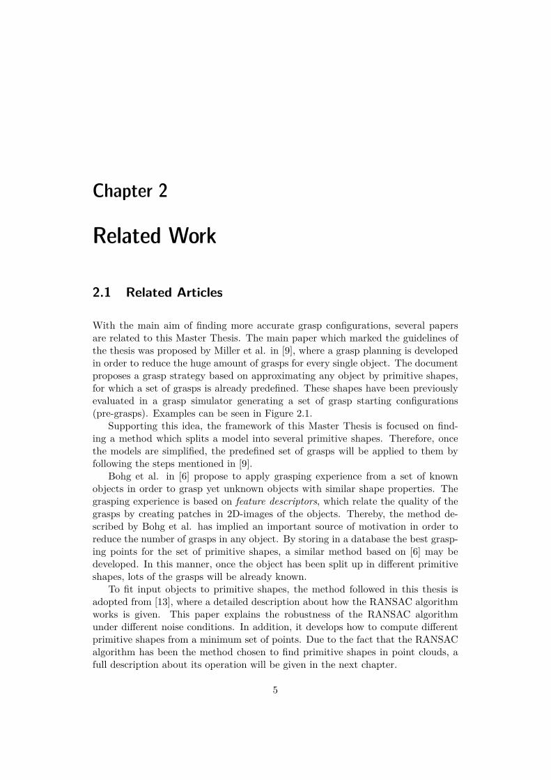
With the main aim of finding more accurate grasp configurations, several papersare related to this Master Thesis. The main paper which marked the guidelines ofthe thesis was proposed by Miller et al. in [9], where a grasp planning is developedin order to reduce the huge amount of grasps for every single object. The documentproposes a grasp strategy based on approximating any object by primitive shapes,for which a set of grasps is already predefined. These shapes have been previouslyevaluated in a grasp simulator generating a set of grasp starting configurations(pre-grasps). Examples can be seen in Figure 2.1.
Supporting this idea, the framework of this Master Thesis is focused on find-ing a method which splits a model into several primitive shapes. Therefore, oncethe models are simplified, the predefined set of grasps will be applied to them byfollowing the steps mentioned in [9].
Bohg et al. in [6] propose to apply grasping experience from a set of knownobjects in order to grasp yet unknown objects with similar shape properties. Thegrasping experience is based on feature descriptors, which relate the quality of thegrasps by creating patches in 2D-images of the objects. Thereby, the method de-scribed by Bohg et al. has implied an important source of motivation in order toreduce the number of grasps in any object. By storing in a database the best grasp-ing points for the set of primitive shapes, a similar method based on [6] may bedeveloped. In this manner, once the object has been split up in different primitiveshapes, lots of the grasps will be already known.
To fit input objects to primitive shapes, the method followed in this thesis isadopted from [13], where a detailed description about how the RANSAC algorithmworks is given. This paper explains the robustness of the RANSAC algorithmunder different noise conditions. In addition, it develops how to compute differentprimitive shapes from a minimum set of points. Due to the fact that the RANSACalgorithm has been the method chosen to find primitive shapes in point clouds, afull description about its operation will be given in the next chapter.
5
6 CHAPTER 2. RELATED WORK
Besides the RANSAC algorithm, there is another iteration method to alignfree-form shapes known as ICP algorithm. This method was developed by Besl andMcKay in [4] and it tries to find the transformation between a point cloud and somereference surfaces in several iterations. In each iteration, the algorithm selects theclosest points as correspondences and computes the transformation for minimizingthe square errors between each of the reference surfaces and the model which isbeing estimated. In [11] Rusinkiewicz and Levoy describe some efficient variants ofthe ICP algorithm. Although this algorithm fulfills the requirements of fitting pointclouds to primitive shapes, the decision of using RANSAC instead of ICP was dueto the fact that the first one works better under hard noise conditions.
In [12] the use of primitives shapes is suggested to reconstruct incomplete pointclouds. The proposed method decomposes a point cloud into several primitiveshapes by using the RANSAC algorithm. Afterwards a Primitive adherence phaseis applied together with a Primitive connectivity phase. The Primitive adherencephase creates an energy function that assigns any closed surface a cost according tohow well the surface adheres to a given set of primitive shapes. In the Primitive con-nectivity phase a method is applied that ensures which surface parts correspondingto a single primitive, form a connected subset of the reconstructed surface. There-fore, regarding the Master Thesis, the most helpful part in the mentioned documentis the Primitive adherence phase, since once the RANSAC algorithm has found thebest candidate form for each primitive shape, a decision criterion is necessary todecide which primitive shape fits the point cloud best.
(a) (b) (c) (d)
Figure 2.1: Grasp generation points on primitive shapes. Picture copied from [9]
2.2 The BoxDecomposition AlgorithmDue to the wide range of models existing in the real world and the numerous grapsthat can be applied to them, it is inconceivable to store all this in a database. Inorder to make the search for good grasps much more efficient, Hübner et al. proposedin [8] to split up point clouds (coming for example from stereo cameras) into boxesto reduce the number of grasps. The BoxDecomposition algorithm is a fit-and-splitmethod where an input model is divided into cuboids, thereby the grasping task is
2.3. THE RANSAC ALGORITHM 7
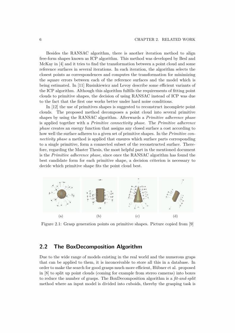
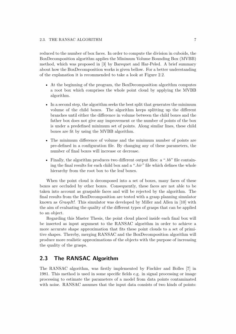
reduced to the number of box faces. In order to compute the division in cuboids, theBoxDecomposition algorithm applies the Minimum Volume Bounding Box (MVBB)method, which was proposed in [3] by Barequet and Har-Peled. A brief summaryabout how the BoxDecomposition works is given bellow. For a better understandingof the explanation it is recommended to take a look at Figure 2.2.
• At the beginning of the program, the BoxDecomposition algorithm computesa root box which comprises the whole point cloud by applying the MVBBalgorithm.
• In a second step, the algorithm seeks the best split that generates the minimumvolume of the child boxes. The algorithm keeps splitting up the differentbranches until either the difference in volume between the child boxes and thefather box does not give any improvement or the number of points of the boxis under a predefined minimum set of points. Along similar lines, these childboxes are fit by using the MVBB algorithm.
• The minimum difference of volume and the minimum number of points arepre-defined in a configuration file. By changing any of these parameters, thenumber of final boxes will increase or decrease.
• Finally, the algorithm produces two different output files: a “.bb” file contain-ing the final results for each child box and a “.hir” file which defines the wholehierarchy from the root box to the leaf boxes.
When the point cloud is decomposed into a set of boxes, many faces of theseboxes are occluded by other boxes. Consequently, these faces are not able to betaken into account as graspable faces and will be rejected by the algorithm. Thefinal results from the BoxDecomposition are tested with a grasp planning simulatorknown as GraspIt!. This simulator was developed by Miller and Allen in [10] withthe aim of evaluating the quality of the different types of grasps that can be appliedto an object.
Regarding this Master Thesis, the point cloud placed inside each final box willbe inserted as input argument to the RANSAC algorithm in order to achieve amore accurate shape approximation that fits these point clouds to a set of primi-tive shapes. Thereby, merging RANSAC and the BoxDecomposition algorithm willproduce more realistic approximations of the objects with the purpose of increasingthe quality of the grasps.
2.3 The RANSAC AlgorithmThe RANSAC algorithm, was firstly implemented by Fischler and Bolles [7] in1981. This method is used in some specific fields e.g. in signal processing or imageprocessing to estimate the parameters of a model from data points contaminatedwith noise. RANSAC assumes that the input data consists of two kinds of points:
8 CHAPTER 2. RELATED WORK
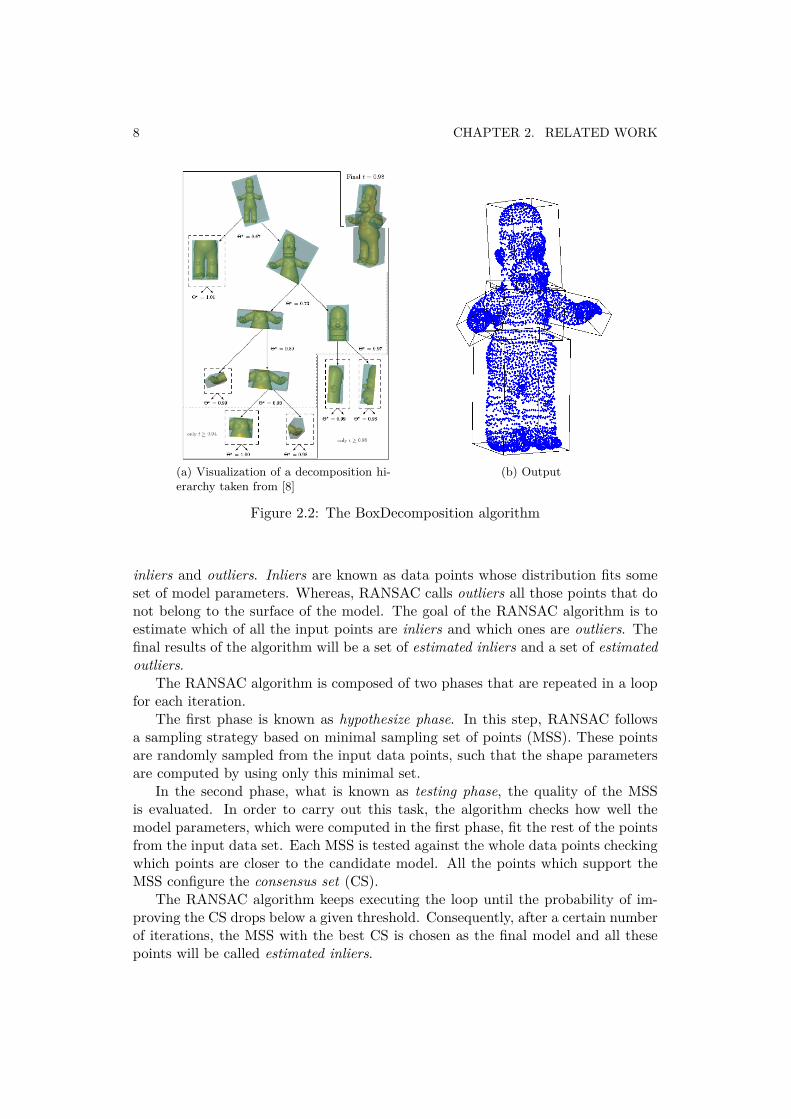
(a) Visualization of a decomposition hi-erarchy taken from [8]
(b) Output
Figure 2.2: The BoxDecomposition algorithm
inliers and outliers. Inliers are known as data points whose distribution fits someset of model parameters. Whereas, RANSAC calls outliers all those points that donot belong to the surface of the model. The goal of the RANSAC algorithm is toestimate which of all the input points are inliers and which ones are outliers. Thefinal results of the algorithm will be a set of estimated inliers and a set of estimatedoutliers.
The RANSAC algorithm is composed of two phases that are repeated in a loopfor each iteration.
The first phase is known as hypothesize phase. In this step, RANSAC followsa sampling strategy based on minimal sampling set of points (MSS). These pointsare randomly sampled from the input data points, such that the shape parametersare computed by using only this minimal set.
In the second phase, what is known as testing phase, the quality of the MSSis evaluated. In order to carry out this task, the algorithm checks how well themodel parameters, which were computed in the first phase, fit the rest of the pointsfrom the input data set. Each MSS is tested against the whole data points checkingwhich points are closer to the candidate model. All the points which support theMSS configure the consensus set (CS).
The RANSAC algorithm keeps executing the loop until the probability of im-proving the CS drops below a given threshold. Consequently, after a certain numberof iterations, the MSS with the best CS is chosen as the final model and all thesepoints will be called estimated inliers.
2.3. THE RANSAC ALGORITHM 9
RANSAC algorithm is capable of finding models even if the 50% of the inputdata set is contaminated by noise points. This fact was demonstrated by Zuliani in[16], and moreover it will be shown in the Experimental Evaluation Chapter (4) foreach primitive shape.
2.3.1 RANSAC nomenclatureA summary of the main RANSAC parameters is given in this subsection. Thenomenclature is based on [16].
• D: It is the input data set which is composed of N points D = {p1, p2, ...pN}.This set represents all data points which will be evaluated by RANSAC.
• MSS: Minimal Sample Set. It is the necessary set of points to compute theparameters which define a model. These points are randomly sampled fromthe input dataset D.
• k: This value defines the cardinality of the MSS. The cardinality of a modelis the minimal number of points that are necessary to compute it.
• Theta: It is the set of parameters that defines a model obtained by applyingthe estimation function to the MSS. Depending on the nature of the modelthat is estimated, these parameters can be the radius, center, hight, width,directional vector, etc.
• δ: Error Threshold. It is responsible for judging which points from D belongto the estimated model. The error of each point with regard to the MSS iscompared with this threshold to form the CS.
• CS: Consensus Set. Set of points of all those elements in D which are consis-tent with the evaluated model. All those points whose error (with regard tothe estimated model) is under the value of δ will be labeled as CS elements.
• J: CS Cost. Parameter which evaluates the cost of a CS regarding the errorof all the points to the estimated model. This value is calculated by MSAC, avariation of RANSAC implemented by Torr and Zissermann in [15], to measurethe quality of the obtained CSs.
2.3.2 RANSAC variationsIn order to improve the original RANSAC algorithm, some variations have beenproposed. Two modifications of RANSAC are implemented by Torr et al. in [15]called MSAC and MLESAC. In contrast to the original formulation of RANSACproposed by Fischler and Bolles in [7], where the ranking of a CS was nothing butits cardinality, in these variations, besides the cardinality of the CS, they take intoaccount the quality of this set by computing its likelihood. Therefore in MSAC theCS is evaluated according to how the estimated inliers fit to the estimated model by

10 CHAPTER 2. RELATED WORK
using M-estimators. By contrast, MLESAC sorts out the CSs by computing theirlikelihoods, choosing as the best CS that one which maximizes the likelihood of thesolution. The MSAC variation has been applied in this Master Thesis to improvethe choice of the final solution.
In [14] Tordoff gives a modification of MLESAC, known as Guided-MLESAC.This algorithm uses the input information in order to make guided sampling basedon other knowledge from the images instead of making iterative random sampling.
In a similar way, Chum in [5] proposes the PROSAC algorithm as a variation ofRANSAC. This algorithm exploits the linear ordering defined on the set of corre-spondences by a similarity function used in establishing tentative correspondences.PROSAC is faster than RANSAC and converges toward it in the worst case.
Chapter 3
Fitting Primitive Shapes to Point Clouds
3.1 RANSAC in MatLab
In this section is going to be introduced how RANSAC works in Matlab [2]. For thispurpose, when a program is designed in Matlab to be able to use it together with theRANSAC algorithm, some configurations parameters have to be set at the beginningof the program. In the configuration part, the user defines the performance of theprogram according to the purpose for which is going to be executed. Once theseoptions have been set, the RANSAC algorithm is run along with the D pointsand the configuration settings. Both of them are used as input arguments for theRANSAC core program.
When the main program (the RANSAC core function) gets started, the config-uration settings are evaluated according to our requirements. Furthermore, in thestarting phase two important Matlab functions, which are related with the modelthat we want to find, are defined. The first one is called the estimation function(Subsection 3.1.2), which is the program responsible for computing the primitiveshape from the MSS given. The second one is known as the error function (Sub-section 3.1.3), which is the program in charge of checking how good the candidatemodel (previously computed by the estimation function) is with regard to the pointcloud. Thereby, if a new primitive shape wants to be found in a point cloud, it isonly necessary to create these two functions.
Once the set up phase is over, the RANSAC algorithm needs to know the cardi-nality of the MSS (k). This value is defined in the estimation function of each model.Therefore, the estimation function is called at the beginning of the RANSAC corealgorithm with the aim of defining the cardinality of the minimal sample set (MSS).
Besides the k value, an error threshold is set. This threshold is defined in theerror function and its value depends on the shape that we want to find. Thus, allthose points (from D) whose error with respect to the estimated shape is under theerror threshold will be selected as estimated inliers.
11
12 CHAPTER 3. FITTING PRIMITIVE SHAPES TO POINT CLOUDS
3.1.1 Main loop phase
The main loop starts sampling the minimal sample set (MSS) and the main param-eters which define the shape (Theta):
The MSS represents a subset of points taken randomly from the input set ofpoints (D). The size of the MSS is defined by k (cardinality of the shape).
When the MSS has been obtained, this set is sent to the estimation function inorder to compute the candidate shape. The output of the estimation function willbe contained in Theta. The parameters of this set define the candidate shape thatis going to be evaluated.
Once the Theta is computed, the evaluation of this one has to be carried out.For this purpose, RANSAC calls to the error function to determine the error of eachpoint of D with regard to the candidate shape. This error represents the distancefrom the surface of the shape to the points. Therefore, a different error is obtainedfor each point of D. In order to decide which points might belong to the surface,every single error is compared with the threshold, creating a consensus set (CS).
With the aim of obtaining the quality of the CS, the cost of this one is estimatedtaking into account the error of all the points to the estimated model. The parameterthat defines the quality of the CS is known as J.
Therefore, when the CS and J have been computed, an evaluation criterionfor these parameters is executed in order to compare the old values with the newones. If any of them is improved, the algorithm will update the old values by thenew ones, otherwise the new values will be preserved. In case that the improvedparameter was the number of CS points, a new number of iterations is calculated(these conditions are fixed at the beginning of the loop).
The main loop will keep executing until either the maximum number of iterationshas been exceeded or the maximum number of no updates is over.
Finally, once the main loop has finished, the RANSAC algorithm gives backthe results to the program which called it previously. These results will containthe parameters of the winning MSS (estimated shape) and the set of points of D(estimated inliers) that best fits into the desired shape.
3.1.2 Primitive shape estimation function
In order to be able to estimate a new geometric shape with the RANSAC algorithm,an estimation program based on the new shape have to be created. In Matlabthis program is implemented by a function which computes the new model from aminimal set of points (MSS).
To estimate the primitive shapes, four estimation functions were designed. Eachfunction consists of a Matlab program that by using k points computes the param-eters of a primitive shape. The mathematical calculations used for each primitiveshape are described in detail in Section 3.2.
The parameters defining the primitive shape are stored in an array known asTheta. This set of data is the output argument of the estimation function and will
3.2. PRIMITIVE SHAPES ESTIMATION ALGORITHMS 13
be evaluated in the error function with the purpose of checking the feasibility of thecandidate shape.
3.1.3 Primitive shape error function
For each estimation program an error function must be created. The main aim ofthis function is the evaluation of Theta.
Once Theta has been obtained by the estimation algorithm, the error functionwill evaluate the quality of the estimated candidate shape with regard to the Dset of points. For this task, the error of each point of D is computed regardingthe candidate shape. The program takes Theta (input argument) and generates anerror vector (output argument) that consists of the distances from each point to thesurface of the estimated shape.
The algorithm used to compute the quality of the estimated model varies ac-cording to the geometrical features of the primitive shape.
The mathematical calculations utilized for each primitive shape are describedin detail in Section 3.2.
3.2 Primitive shapes estimation algorithms
3.2.1 Sphere estimation algorithm
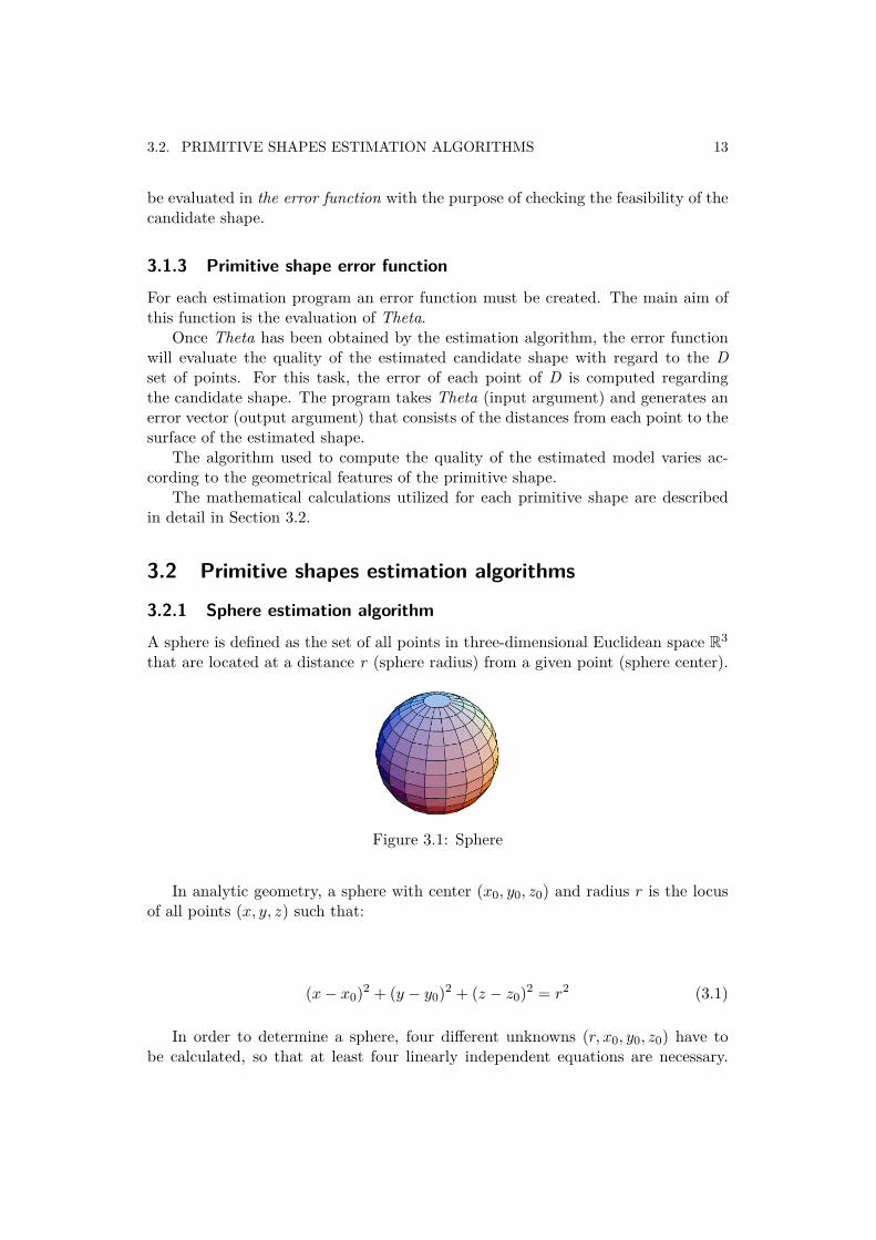
A sphere is defined as the set of all points in three-dimensional Euclidean space R3
that are located at a distance r (sphere radius) from a given point (sphere center).
Figure 3.1: Sphere
In analytic geometry, a sphere with center (x0, y0, z0) and radius r is the locusof all points (x, y, z) such that:
(x− x0)2 + (y − y0)2 + (z − z0)2 = r2 (3.1)
In order to determine a sphere, four different unknowns (r, x0, y0, z0) have tobe calculated, so that at least four linearly independent equations are necessary.
14 CHAPTER 3. FITTING PRIMITIVE SHAPES TO POINT CLOUDS
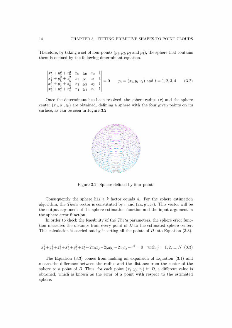
Therefore, by taking a set of four points (p1, p2, p3 and p4), the sphere that containsthem is defined by the following determinant equation.
∣∣∣∣∣∣∣∣∣x2
0 + y20 + z20 x0 y0 z0 1x2
1 + y21 + z21 x1 y1 z1 1x2
3 + y23 + z23 x3 y3 z3 1x2
4 + y24 + z24 x4 y4 z4 1
∣∣∣∣∣∣∣∣∣ = 0 pi = (xi, yi, zi) and i = 1, 2, 3, 4 (3.2)
Once the determinant has been resolved, the sphere radius (r) and the spherecenter (x0, y0, z0) are obtained, defining a sphere with the four given points on itssurface, as can be seen in Figure 3.2
Figure 3.2: Sphere defined by four points
Consequently the sphere has a k factor equals 4. For the sphere estimationalgorithm, the Theta vector is constituted by r and (x0, y0, z0). This vector will bethe output argument of the sphere estimation function and the input argument inthe sphere error function.
In order to check the feasibility of the Theta parameters, the sphere error func-tion measures the distance from every point of D to the estimated sphere center.This calculation is carried out by inserting all the points of D into Equation (3.3).
x2j+y2j+z2j +x2
0+y20 +z20−2x0xj−2y0yj−2z0zj−r2 = 0 with j = 1, 2, ..., N (3.3)
The Equation (3.3) comes from making an expansion of Equation (3.1) andmeans the difference between the radius and the distance from the center of thesphere to a point of D. Thus, for each point (xj , yj , zj) in D, a different value isobtained, which is known as the error of a point with respect to the estimatedsphere.
3.2. PRIMITIVE SHAPES ESTIMATION ALGORITHMS 15
3.2.2 Cylinder estimation algorithm
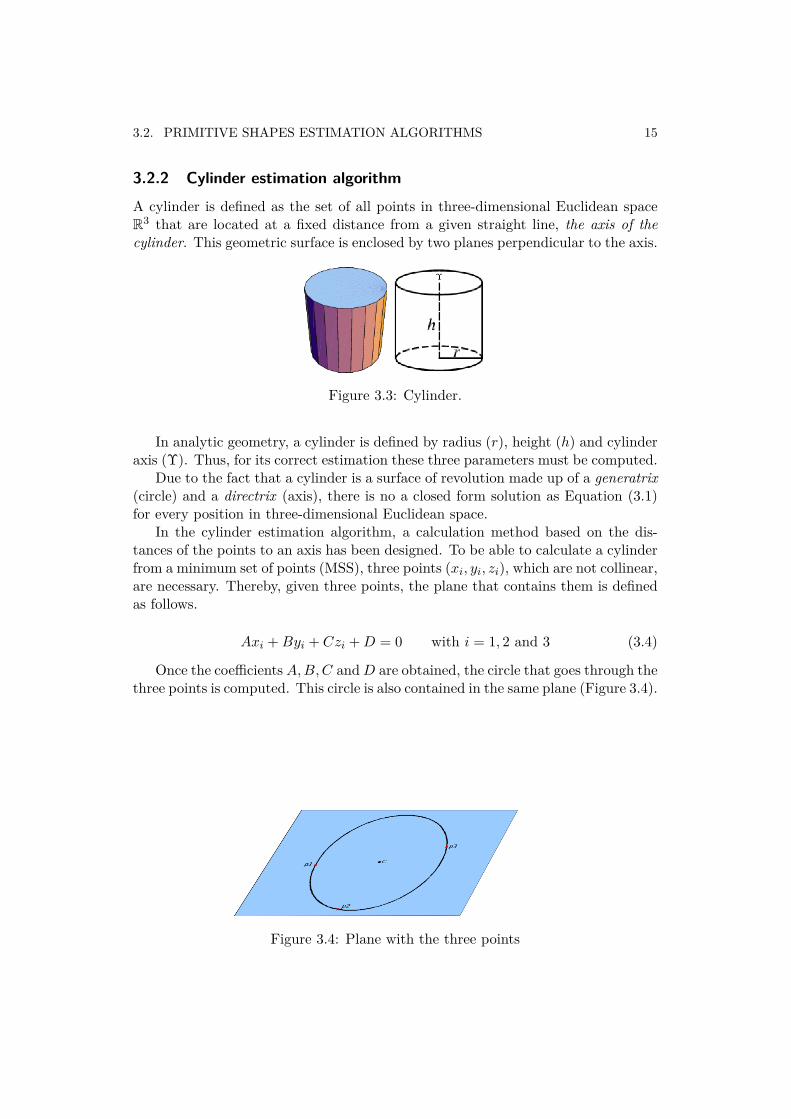
A cylinder is defined as the set of all points in three-dimensional Euclidean spaceR3 that are located at a fixed distance from a given straight line, the axis of thecylinder. This geometric surface is enclosed by two planes perpendicular to the axis.
Figure 3.3: Cylinder.
In analytic geometry, a cylinder is defined by radius (r), height (h) and cylinderaxis (Υ). Thus, for its correct estimation these three parameters must be computed.
Due to the fact that a cylinder is a surface of revolution made up of a generatrix(circle) and a directrix (axis), there is no a closed form solution as Equation (3.1)for every position in three-dimensional Euclidean space.
In the cylinder estimation algorithm, a calculation method based on the dis-tances of the points to an axis has been designed. To be able to calculate a cylinderfrom a minimum set of points (MSS), three points (xi, yi, zi), which are not collinear,are necessary. Thereby, given three points, the plane that contains them is definedas follows.
Axi +Byi + Czi +D = 0 with i = 1, 2 and 3 (3.4)
Once the coefficients A,B,C andD are obtained, the circle that goes through thethree points is computed. This circle is also contained in the same plane (Figure 3.4).
Figure 3.4: Plane with the three points
16 CHAPTER 3. FITTING PRIMITIVE SHAPES TO POINT CLOUDS
Both the radius (r) and the center c = (x0, y0, z0) are obtained by solving thefollowing equations.
d(p1, c) = d(p2, c) = d(p3, c) = r (3.5)
with d(pi, c) =√
(xi − x0)2 + (yi − y0)2 + (zi − z0)2 (3.6)
Therefore, r is designated as the cylinder radius, whereas the cylinder axis isachieved by taking the normal vector of the plane ( ~Un) (previously estimated) andthe center of the circle (x0, y0, z0). These are the necessary parameters to set upthe equation of the straight line Υ which is normal to the plane and goes throughthe center.
Υ ≡
x = x0 + tAy = y0 + tBz = z0 + tC
being ~un = (A,B,C) (3.7)
As a result of these equations, the cylinder cardinality k is 3. Therefore, theTheta vector that describes the cylindrical shape is comprised of three elements ~Un,c and r. The first two define the cylinder axis whereas the last one is the cylinderradius.
By using the radius and the axis of the cylinder, the distance of any point tothe cylindrical surface can be computed. This method will be used to estimate theerror of each point of D to the surface of the cylinder, which is based on computingthe minimum distance (dminj) between each point of D and the cylinder axis.
dminj = | ~un × ~cpD|| ~un|
pD a point of D (3.8)
By subtracting the estimated cylinder radius from these minimum distances, theerror vector Ej is obtained for each point (xj , yj , zj) in D.
Ej = (dminj − r) with Ej ∈ E = [E1, E2, ..., Ej , ...EN ] (3.9)
Once all the errors Ej have been computed, those points whose error is underthe error threshold (δ) will be selected as surface points.
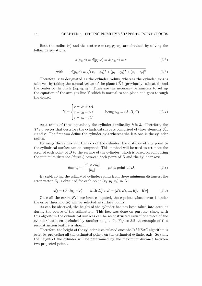
As can be observed, the height of the cylinder has not been taken into accountduring the course of the estimation. This fact was done on purpose, since, withthis algorithm the cylindrical surfaces can be reconstructed even if one piece of thecylinder has been occluded by another shape. In Figure 3.5 an example of thisreconstruction feature is shown.
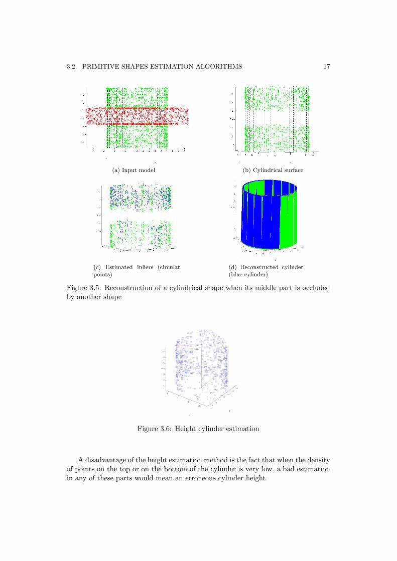
Therefore, the height of the cylinder is calculated once the RANSAC algorithm isover, by projecting all the estimated points on the estimated cylinder axis. So that,the height of the cylinder will be determined by the maximum distance betweentwo projected points.
3.2. PRIMITIVE SHAPES ESTIMATION ALGORITHMS 17
(a) Input model (b) Cylindrical surface
(c) Estimated inliers (circularpoints)
(d) Reconstructed cylinder(blue cylinder)
Figure 3.5: Reconstruction of a cylindrical shape when its middle part is occludedby another shape
−2
0
2
4
−3
−2
−1
0
1
2
3
1
2
3
4
5
6
7
y
x
z
Figure 3.6: Height cylinder estimation
A disadvantage of the height estimation method is the fact that when the densityof points on the top or on the bottom of the cylinder is very low, a bad estimationin any of these parts would mean an erroneous cylinder height.
18 CHAPTER 3. FITTING PRIMITIVE SHAPES TO POINT CLOUDS
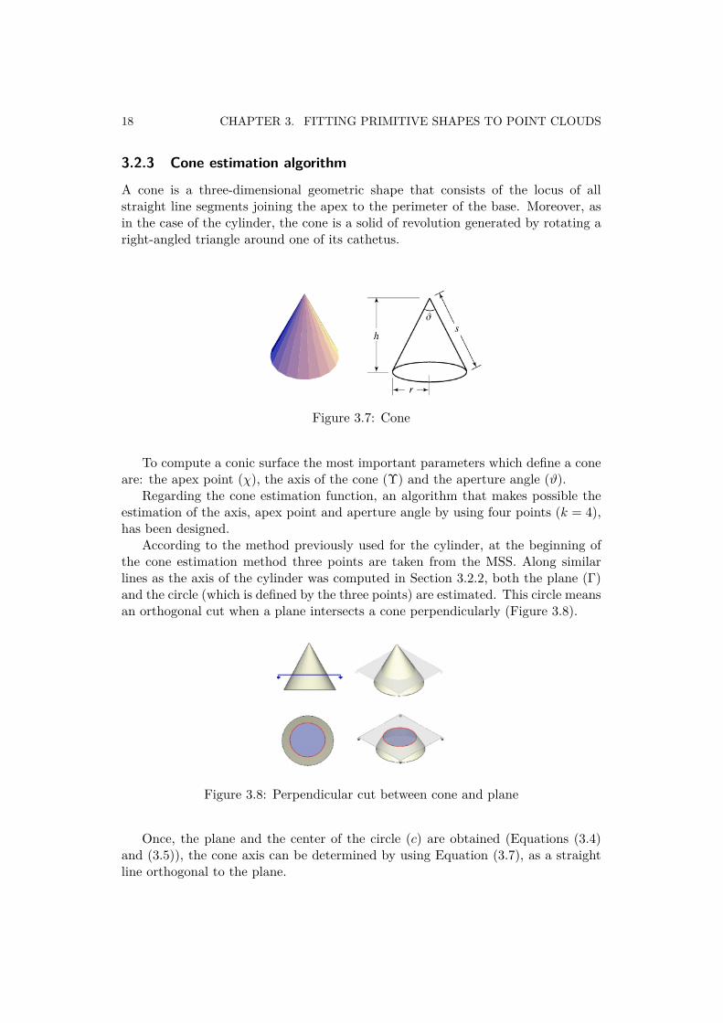
3.2.3 Cone estimation algorithm
A cone is a three-dimensional geometric shape that consists of the locus of allstraight line segments joining the apex to the perimeter of the base. Moreover, asin the case of the cylinder, the cone is a solid of revolution generated by rotating aright-angled triangle around one of its cathetus.
Figure 3.7: Cone
To compute a conic surface the most important parameters which define a coneare: the apex point (χ), the axis of the cone (Υ) and the aperture angle (ϑ).
Regarding the cone estimation function, an algorithm that makes possible theestimation of the axis, apex point and aperture angle by using four points (k = 4),has been designed.
According to the method previously used for the cylinder, at the beginning ofthe cone estimation method three points are taken from the MSS. Along similarlines as the axis of the cylinder was computed in Section 3.2.2, both the plane (Γ)and the circle (which is defined by the three points) are estimated. This circle meansan orthogonal cut when a plane intersects a cone perpendicularly (Figure 3.8).
Figure 3.8: Perpendicular cut between cone and plane
Once, the plane and the center of the circle (c) are obtained (Equations (3.4)and (3.5)), the cone axis can be determined by using Equation (3.7), as a straightline orthogonal to the plane.
3.2. PRIMITIVE SHAPES ESTIMATION ALGORITHMS 19
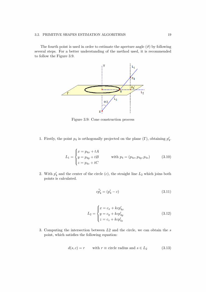
The fourth point is used in order to estimate the aperture angle (ϑ) by followingseveral steps. For a better understanding of the method used, it is recommendedto follow the Figure 3.9.
Figure 3.9: Cone construction process
1. Firstly, the point p4 is orthogonally projected on the plane (Γ), obtaining p′4.
L1 =
x = p4x + tAy = p4y + tBz = p4z + tC
with p4 = (p4x, p4y, p4z) (3.10)
2. With p′4 and the center of the circle (c), the straight line L2 which joins bothpoints is calculated.
~cp′4 = (p′4 − c) (3.11)
L2 =
x = cx + kcp′4xy = cy + kcp′4yz = cz + kcp′4z
(3.12)
3. Computing the intersection between L2 and the circle, we can obtain the spoint, which satisfies the following equation:
d(s, c) = r with r ≡ circle radius and s ∈ L2 (3.13)
20 CHAPTER 3. FITTING PRIMITIVE SHAPES TO POINT CLOUDS
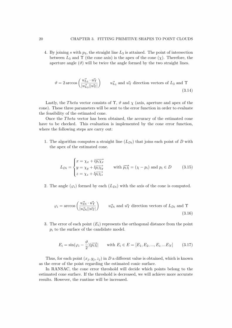
4. By joining s with p4, the straight line L3 is attained. The point of intersectionbetween L3 and Υ (the cone axis) is the apex of the cone (χ). Therefore, theaperture angle (ϑ) will be twice the angle formed by the two straight lines.
ϑ = 2 arccos(~uL3 · ~uΥ| ~uL3 || ~uΥ|
)~uL3 and ~uΥ direction vectors of L3 and Υ
(3.14)
Lastly, the Theta vector consists of Υ, ϑ and χ (axis, aperture and apex of thecone). These three parameters will be sent to the error function in order to evaluatethe feasibility of the estimated cone.
Once the Theta vector has been obtained, the accuracy of the estimated conehave to be checked. This evaluation is implemented by the cone error function,where the following steps are carry out:
1. The algorithm computes a straight line (LDi) that joins each point of D withthe apex of the estimated cone.
LDi =
x = χx + l−−→piχxy = χy + l−−→piχyz = χz + l−−→piχz
with −→piχ = (χ− pi) and pi ∈ D (3.15)
2. The angle (ϕi) formed by each (LDi) with the axis of the cone is computed.
ϕi = arccos(~uDi · ~uΥ| ~uDi|| ~uΥ|
)~uDi and ~uΥ direction vectors of LDi and Υ
(3.16)
3. The error of each point (Ei) represents the orthogonal distance from the pointpi to the surface of the candidate model.
Ei = sin(ϕi −ϑ
2)|−→piχ| with Ei ∈ E = [E1, E2, ..., Ei, ...EN ] (3.17)
Thus, for each point (xj , yj , zj) in D a different value is obtained, which is knownas the error of the point regarding the estimated conic surface.
In RANSAC, the cone error threshold will decide which points belong to theestimated cone surface. If the threshold is decreased, we will achieve more accurateresults. However, the runtime will be increased.
3.2. PRIMITIVE SHAPES ESTIMATION ALGORITHMS 21
3.2.4 Box estimation algorithm
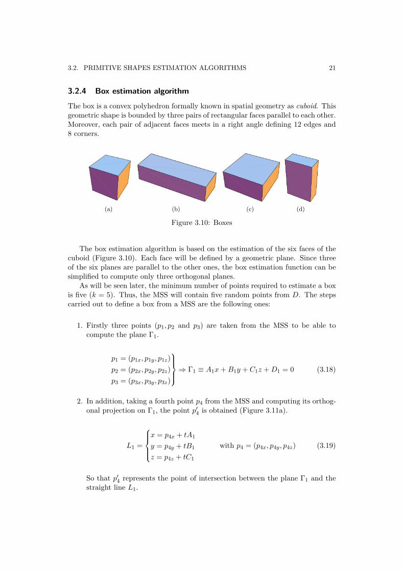
The box is a convex polyhedron formally known in spatial geometry as cuboid. Thisgeometric shape is bounded by three pairs of rectangular faces parallel to each other.Moreover, each pair of adjacent faces meets in a right angle defining 12 edges and8 corners.
(a) (b) (c) (d)
Figure 3.10: Boxes
The box estimation algorithm is based on the estimation of the six faces of thecuboid (Figure 3.10). Each face will be defined by a geometric plane. Since threeof the six planes are parallel to the other ones, the box estimation function can besimplified to compute only three orthogonal planes.
As will be seen later, the minimum number of points required to estimate a boxis five (k = 5). Thus, the MSS will contain five random points from D. The stepscarried out to define a box from a MSS are the following ones:
1. Firstly three points (p1, p2 and p3) are taken from the MSS to be able tocompute the plane Γ1.
p1 = (p1x, p1y, p1z)p2 = (p2x, p2y, p2z)p3 = (p3x, p3y, p3z)
⇒ Γ1 ≡ A1x+B1y + C1z +D1 = 0 (3.18)
2. In addition, taking a fourth point p4 from the MSS and computing its orthog-onal projection on Γ1, the point p′4 is obtained (Figure 3.11a).
L1 =
x = p4x + tA1
y = p4y + tB1
z = p4z + tC1
with p4 = (p4x, p4y, p4z) (3.19)
So that p′4 represents the point of intersection between the plane Γ1 and thestraight line L1.
22 CHAPTER 3. FITTING PRIMITIVE SHAPES TO POINT CLOUDS
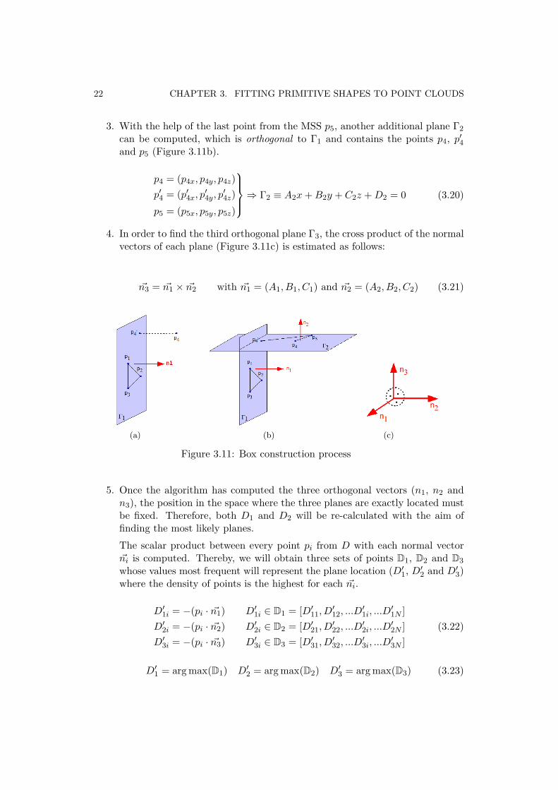
3. With the help of the last point from the MSS p5, another additional plane Γ2can be computed, which is orthogonal to Γ1 and contains the points p4, p′4and p5 (Figure 3.11b).
p4 = (p4x, p4y, p4z)p′4 = (p′4x, p′4y, p′4z)p5 = (p5x, p5y, p5z)
⇒ Γ2 ≡ A2x+B2y + C2z +D2 = 0 (3.20)
4. In order to find the third orthogonal plane Γ3, the cross product of the normalvectors of each plane (Figure 3.11c) is estimated as follows:
~n3 = ~n1 × ~n2 with ~n1 = (A1, B1, C1) and ~n2 = (A2, B2, C2) (3.21)
(a) (b) (c)
Figure 3.11: Box construction process
5. Once the algorithm has computed the three orthogonal vectors (n1, n2 andn3), the position in the space where the three planes are exactly located mustbe fixed. Therefore, both D1 and D2 will be re-calculated with the aim offinding the most likely planes.The scalar product between every point pi from D with each normal vector~ni is computed. Thereby, we will obtain three sets of points D1, D2 and D3whose values most frequent will represent the plane location (D′1, D′2 and D′3)where the density of points is the highest for each ~ni.
D′1i = −(pi · ~n1) D′1i ∈ D1 = [D′11, D′12, ...D
′1i, ...D
′1N ]
D′2i = −(pi · ~n2) D′2i ∈ D2 = [D′21, D′22, ...D
′2i, ...D
′2N ]
D′3i = −(pi · ~n3) D′3i ∈ D3 = [D′31, D′32, ...D
′3i, ...D
′3N ]
(3.22)
D′1 = arg max(D1) D′2 = arg max(D2) D′3 = arg max(D3) (3.23)
3.2. PRIMITIVE SHAPES ESTIMATION ALGORITHMS 23
By calculating the new values of D1 and D2, the RANSAC algorithm will savelots of iterations. Consequently, the overall runtime will be decreased.
Mode RunTime (s)With D′1 & D′2 19.6552With D1 & D2 53.1721
In one RANSAC iteration are estimated three orthogonal planes by using a MSSwith k = 5, so the Theta vector will be made up of Γ′1, Γ′2 and Γ′3.
Γ′1 ≡ A1x+B1y + C1z +D′1 = 0Γ′2 ≡ A2x+B2y + C2z +D′2 = 0Γ′3 ≡ A3x+B3y + C3z +D′3 = 0
⇒ Γ′1 ⊥ Γ′2 ⊥ Γ′3 (3.24)
In order to evaluate the error of the Theta vector regarding the whole pointcloud D, an error function, which consists of two steps, has been developed:
1. Firstly, every point belonging to the point cloud is inserted in each one of thethree plane equations. In this manner, a point pi generates three differenterror values E1i, E2i and E3i, which mean how far the point is from each ofthe planes.
E1i = A1pix +B1piy + C1piz +D′1; E1i ∈ E1 = [E11, E12, ...E1i, ...E1N ]E2i = A2pix +B2piy + C2piz +D′2; E2i ∈ E2 = [E21, E22, ...E2i, ...E2N ]E3i = A3pix +B3piy + C3piz +D′3; E3i ∈ E3 = [E31, E32, ...E3i, ...E3N ]
(3.25)
2. Secondly, despite the fact that three errors are obtained for each point pi,solely the lowest value will represent the real error of the point with regard tothe surface of the box.
E = [min(E11, E21, E31),min(E12, E22, E32), ...min(E1i, E2i, E3i), ......min(E1N , E2N , E3N )]
(3.26)
As mentioned above, a box is defined by three pairs of rectangular faces placedopposite each other. Once the RANSAC algorithm has found the three main planes(faces), the search for the parallel planes have to be carried out. This task isimplemented in a similar way as the main planes were computed. Basing on thefact that the parallel planes have the same normal vectors as Γ′1, Γ′2 and Γ′3, theestimation process of these ones is simplified to the search of D4, D5 and D6 (theposition factors of the planes in the space).
24 CHAPTER 3. FITTING PRIMITIVE SHAPES TO POINT CLOUDS
Consequently, the scalar product between each normal vector and the pointcloud is computed again with the aim of finding the most frequent planes. Nev-ertheless, this time the point cloud consists only of those points which were notestimated as inliers of the already estimated planes.
Even though this method works correctly in ideal conditions (low noise environ-ments), the results of the tests have shown that the method fails when the amountof noise in the point cloud is considerable. Thus, a noise filter has been applied toimprove the results in hard noise conditions.
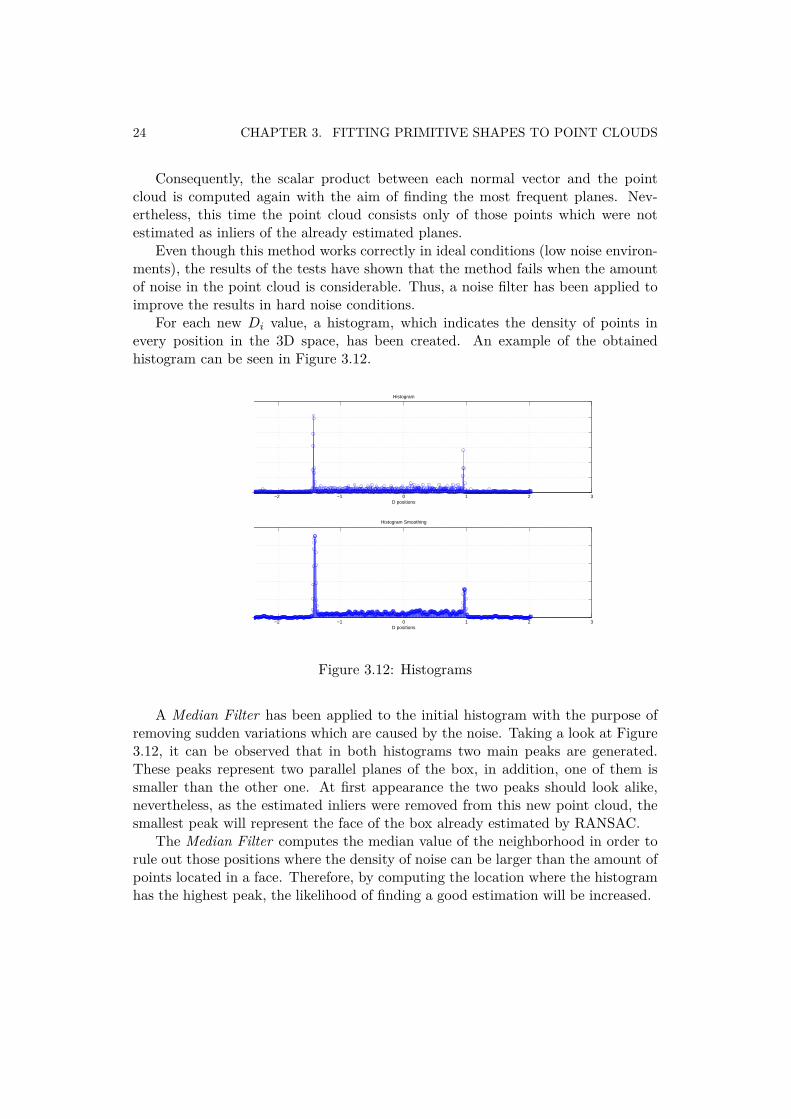
For each new Di value, a histogram, which indicates the density of points inevery position in the 3D space, has been created. An example of the obtainedhistogram can be seen in Figure 3.12.
−2 −1 0 1 2 3
Histogram
D positions
−2 −1 0 1 2 3
Histogram Smoothing
D positions
Figure 3.12: Histograms
A Median Filter has been applied to the initial histogram with the purpose ofremoving sudden variations which are caused by the noise. Taking a look at Figure3.12, it can be observed that in both histograms two main peaks are generated.These peaks represent two parallel planes of the box, in addition, one of them issmaller than the other one. At first appearance the two peaks should look alike,nevertheless, as the estimated inliers were removed from this new point cloud, thesmallest peak will represent the face of the box already estimated by RANSAC.
The Median Filter computes the median value of the neighborhood in order torule out those positions where the density of noise can be larger than the amount ofpoints located in a face. Therefore, by computing the location where the histogramhas the highest peak, the likelihood of finding a good estimation will be increased.
Chapter 4
Experimental Evaluation
In order to obtain the feasibility of the RANSAC designed algorithms, a set of test,whose main goal is to check the accuracy of the primitive shape detection whenfacing a point cloud that is corrupted by noise, has been programmed. These testsare based on the insertion of a primitive shape with an amount of noise as inputparameter in the RANSAC estimation.
With the aim of achieving more realistic results, these tests use different kindsof noise. Although there are many types of noise that could have been applied tothe test. It was eventually decided to use just two kinds of noise based on uniformdistribution functions. Since the approach is aimed at using it with point cloudsobtained from a stereo camera, the noise must be modeled accordingly.
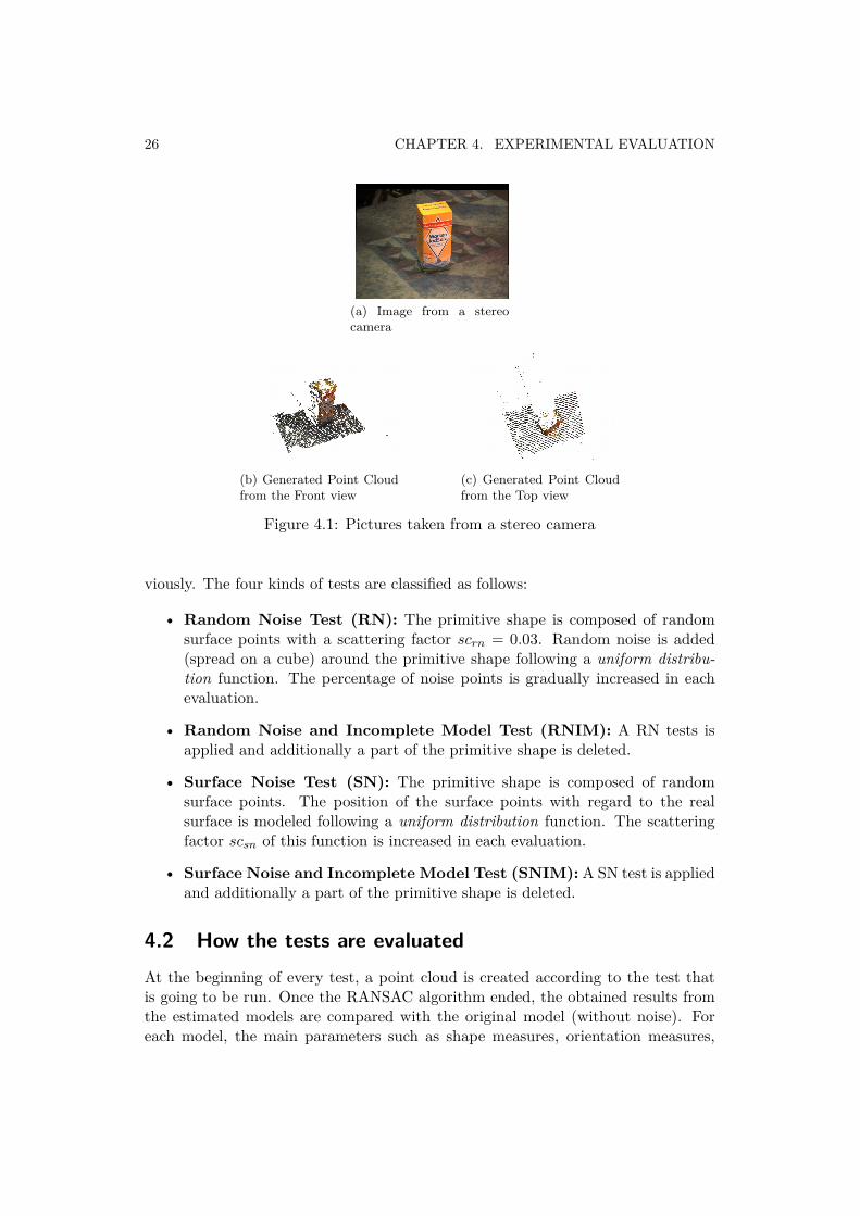
The first kind of noise used is called Random Noise (RN) that is spread outuniformly surrounded the primitive shape. The RN simulates the noise points ona model, which can be caused e.g. by errors in the stereo matching process. Anexample of a typical point cloud obtained from a stereo camera is given in Figure4.1.
The second kind of noise is called Surface Noise (SN). In this case, the uniformnoise distribution is applied to points on the surface of the primitive shape. Thisnoise defines the blurring of the model caused by a stereo camera on the surface ofthis one. In other words, the surface of the primitive shape is blurred by applyingthis kind of noise with the purpose of representing real models obtained from astereo camera. An example of an image with surface noise from a stereo camera isgiven in Figures 4.1b and 4.1c.
In addition to the different kinds of noise implemented, in two of the four tests,incomplete point clouds are used, because a camera can usually see only the frontside of the shape if not moved around it (as it shown in Figure 4.1a).
4.1 Test scenarios
To evaluate the feasibility of each primitive shape estimation algorithm with RANSAC,it was necessary to create four different scenarios based on the mentioned ones pre-
25
26 CHAPTER 4. EXPERIMENTAL EVALUATION
(a) Image from a stereocamera
(b) Generated Point Cloudfrom the Front view
(c) Generated Point Cloudfrom the Top view
Figure 4.1: Pictures taken from a stereo camera
viously. The four kinds of tests are classified as follows:
• Random Noise Test (RN): The primitive shape is composed of randomsurface points with a scattering factor scrn = 0.03. Random noise is added(spread on a cube) around the primitive shape following a uniform distribu-tion function. The percentage of noise points is gradually increased in eachevaluation.
• Random Noise and Incomplete Model Test (RNIM): A RN tests isapplied and additionally a part of the primitive shape is deleted.
• Surface Noise Test (SN): The primitive shape is composed of randomsurface points. The position of the surface points with regard to the realsurface is modeled following a uniform distribution function. The scatteringfactor scsn of this function is increased in each evaluation.
• Surface Noise and Incomplete Model Test (SNIM): A SN test is appliedand additionally a part of the primitive shape is deleted.
4.2 How the tests are evaluatedAt the beginning of every test, a point cloud is created according to the test thatis going to be run. Once the RANSAC algorithm ended, the obtained results fromthe estimated models are compared with the original model (without noise). Foreach model, the main parameters such as shape measures, orientation measures,
4.3. TEST RESULTS 27
runtimes and number of estimated inliers are checked. In order to achieve a greaternumber of results, a set of values has been defined for each kind of test.
For RN and RNIM tests, six percentages of noise versus surface points are set:
{10, 20, 30, 40, 50, 60} (%)
These percentages represent the amount of noise points that has been inserted in thepoint cloud. The remaining percentages define the points which model the surfaceof the primitive shape. As it can be seen, the amount of noise points is increasedin each evaluation.
For the SN and SNDI tests, six different scattering factors scsn are set:
scsn = {0.010, 0.050, 0.075, 0.100, 0125, 0.150}
The uniform function models the distance of the points to the real surface. Thescattering factor is increased in each iteration making the surface of the primitiveshape increasingly distorted.
By evaluating each element from the sets, the strength of the estimation meth-ods can be checked. In order to achieve more reliable results, each percentage orscattering factor has been evaluated ten times. Thereby, the results used in tablesand graphs are the average results of each evaluation.
Lastly, in the four tests, the total number of points, which define the point cloud,has been fixed to 1500.
4.3 Test results
4.3.1 Sphere algorithm evaluationIn order to evaluate the accuracy of the RANSAC method applied to a geometricsphere, the different scenarios mentioned above are going to be used. During thesimulations, a random center and a random radius have been set, these values arekept in the four tests.
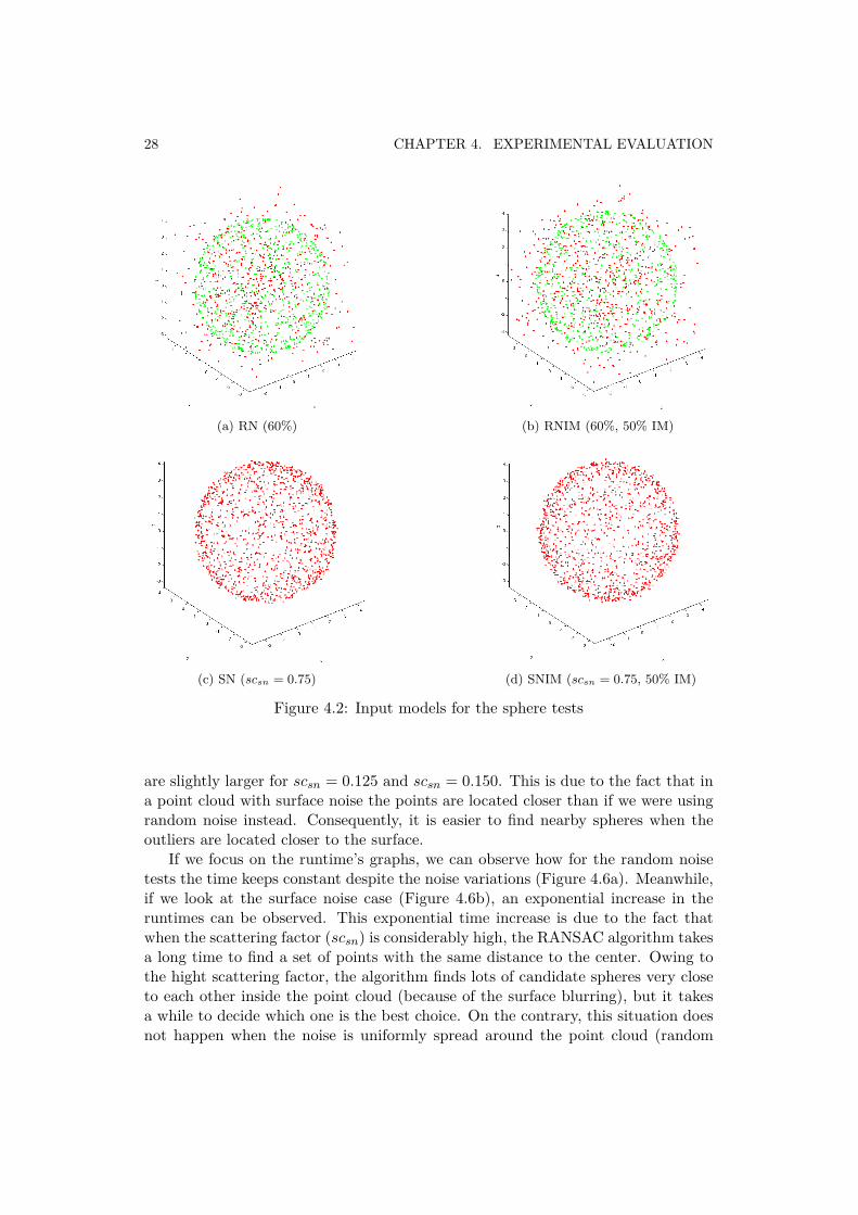
The input data points used in each test can be seen in Figure 4.2.Moreover, in Figures 4.3 and 4.4 several examples with the outputs of each test
are shown.For the representation of the incomplete models, 50% of the sphere has been
deleted in the RNIM and SNIM tests. This fact shows the reliability of the sphereestimation algorithm under hard occlusion conditions.
As we can see in Figure 4.5, the errors got for both the radius and center ofthe sphere are quite small, given to this method a big accuracy. Furthermore, if wefocus on the surface noise tests, it can be observed that the radius and center errors
28 CHAPTER 4. EXPERIMENTAL EVALUATION
(a) RN (60%) (b) RNIM (60%, 50% IM)
(c) SN (scsn = 0.75) (d) SNIM (scsn = 0.75, 50% IM)
Figure 4.2: Input models for the sphere tests
are slightly larger for scsn = 0.125 and scsn = 0.150. This is due to the fact that ina point cloud with surface noise the points are located closer than if we were usingrandom noise instead. Consequently, it is easier to find nearby spheres when theoutliers are located closer to the surface.
If we focus on the runtime’s graphs, we can observe how for the random noisetests the time keeps constant despite the noise variations (Figure 4.6a). Meanwhile,if we look at the surface noise case (Figure 4.6b), an exponential increase in theruntimes can be observed. This exponential time increase is due to the fact thatwhen the scattering factor (scsn) is considerably high, the RANSAC algorithm takesa long time to find a set of points with the same distance to the center. Owing tothe hight scattering factor, the algorithm finds lots of candidate spheres very closeto each other inside the point cloud (because of the surface blurring), but it takesa while to decide which one is the best choice. On the contrary, this situation doesnot happen when the noise is uniformly spread around the point cloud (random
4.3. TEST RESULTS 29
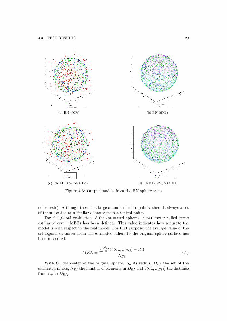
(a) RN (60%) (b) RN (60%)
(c) RNIM (60%, 50% IM) (d) RNIM (60%, 50% IM)
Figure 4.3: Output models from the RN sphere tests
noise tests). Although there is a large amount of noise points, there is always a setof them located at a similar distance from a central point.
For the global evaluation of the estimated spheres, a parameter called meanestimated error (MEE) has been defined. This value indicates how accurate themodel is with respect to the real model. For that purpose, the average value of theorthogonal distances from the estimated inliers to the original sphere surface hasbeen measured.
MEE =∑NEIj=1 (d(Co, DEIj)−Ro)
NEI(4.1)
With Co the center of the original sphere, Ro its radius, DEI the set of theestimated inliers, NEI the number of elements in DEI and d(Co, DEIj) the distancefrom Co to DEIj .
30 CHAPTER 4. EXPERIMENTAL EVALUATION
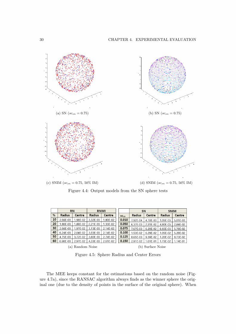
(a) SN (scsn = 0.75) (b) SN (scsn = 0.75)
(c) SNIM (scsn = 0.75, 50% IM) (d) SNIM (scsn = 0.75, 50% IM)
Figure 4.4: Output models from the SN sphere tests
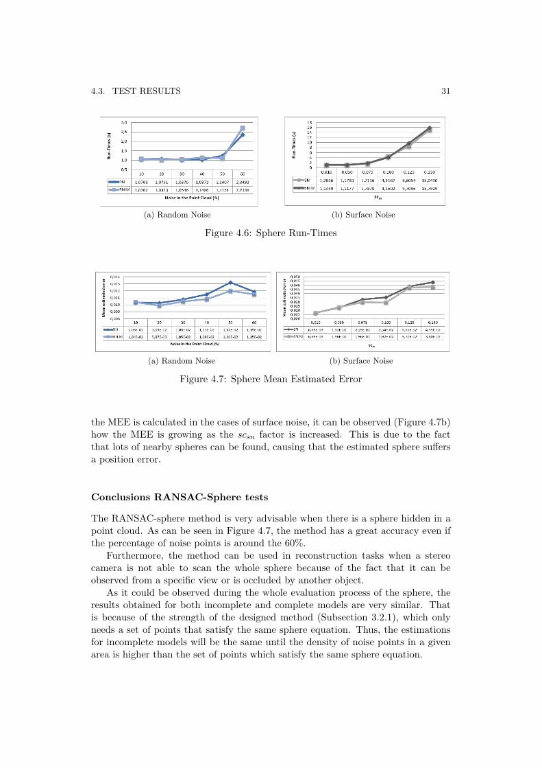
(a) Random Noise (b) Surface Noise
Figure 4.5: Sphere Radius and Center Errors
The MEE keeps constant for the estimations based on the random noise (Fig-ure 4.7a), since the RANSAC algorithm always finds as the winner sphere the orig-inal one (due to the density of points in the surface of the original sphere). When
4.3. TEST RESULTS 31
(a) Random Noise (b) Surface Noise
Figure 4.6: Sphere Run-Times
(a) Random Noise (b) Surface Noise
Figure 4.7: Sphere Mean Estimated Error
the MEE is calculated in the cases of surface noise, it can be observed (Figure 4.7b)how the MEE is growing as the scsn factor is increased. This is due to the factthat lots of nearby spheres can be found, causing that the estimated sphere suffersa position error.
Conclusions RANSAC-Sphere tests
The RANSAC-sphere method is very advisable when there is a sphere hidden in apoint cloud. As can be seen in Figure 4.7, the method has a great accuracy even ifthe percentage of noise points is around the 60%.
Furthermore, the method can be used in reconstruction tasks when a stereocamera is not able to scan the whole sphere because of the fact that it can beobserved from a specific view or is occluded by another object.
As it could be observed during the whole evaluation process of the sphere, theresults obtained for both incomplete and complete models are very similar. Thatis because of the strength of the designed method (Subsection 3.2.1), which onlyneeds a set of points that satisfy the same sphere equation. Thus, the estimationsfor incomplete models will be the same until the density of noise points in a givenarea is higher than the set of points which satisfy the same sphere equation.
32 CHAPTER 4. EXPERIMENTAL EVALUATION
4.3.2 Cylinder algorithm evaluation
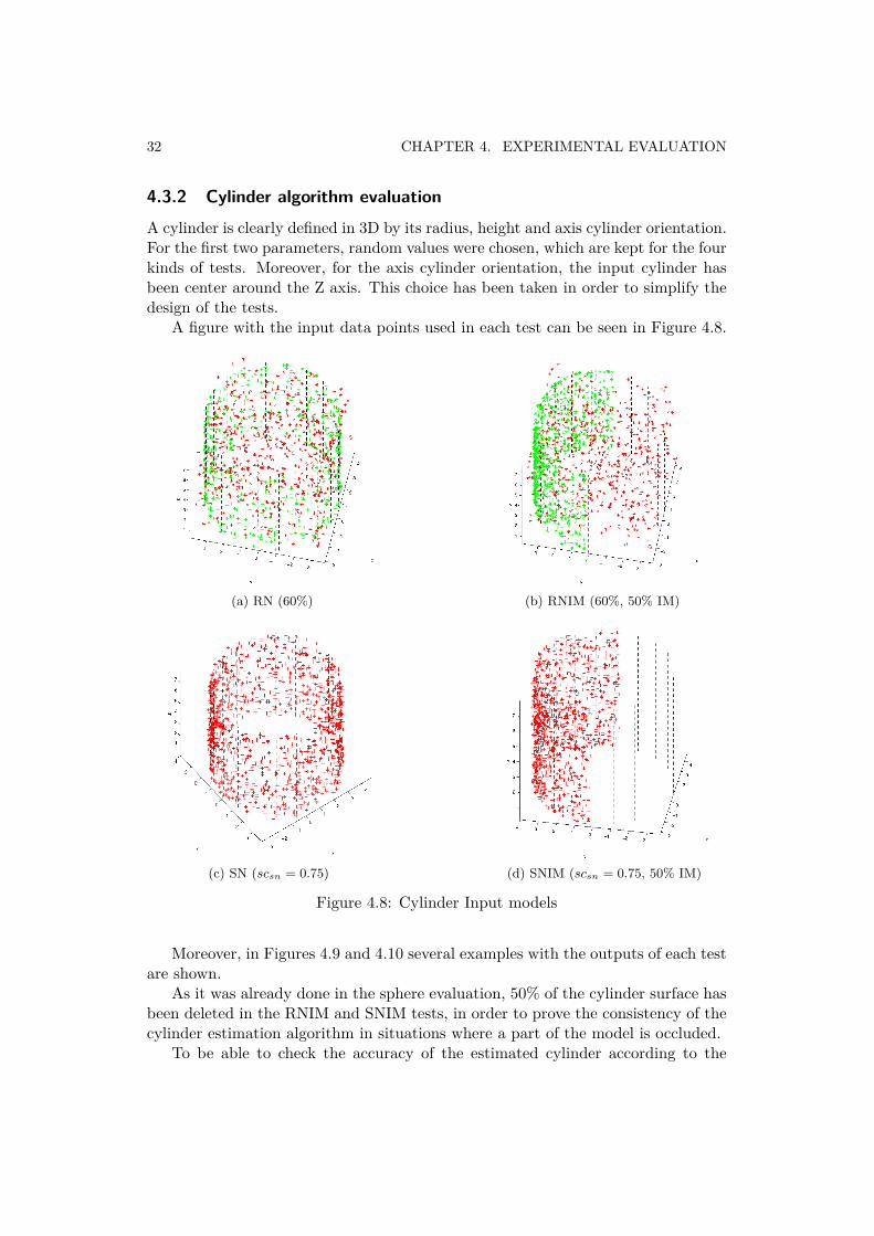
A cylinder is clearly defined in 3D by its radius, height and axis cylinder orientation.For the first two parameters, random values were chosen, which are kept for the fourkinds of tests. Moreover, for the axis cylinder orientation, the input cylinder hasbeen center around the Z axis. This choice has been taken in order to simplify thedesign of the tests.
A figure with the input data points used in each test can be seen in Figure 4.8.
(a) RN (60%) (b) RNIM (60%, 50% IM)
(c) SN (scsn = 0.75) (d) SNIM (scsn = 0.75, 50% IM)
Figure 4.8: Cylinder Input models
Moreover, in Figures 4.9 and 4.10 several examples with the outputs of each testare shown.
As it was already done in the sphere evaluation, 50% of the cylinder surface hasbeen deleted in the RNIM and SNIM tests, in order to prove the consistency of thecylinder estimation algorithm in situations where a part of the model is occluded.
To be able to check the accuracy of the estimated cylinder according to the
4.3. TEST RESULTS 33
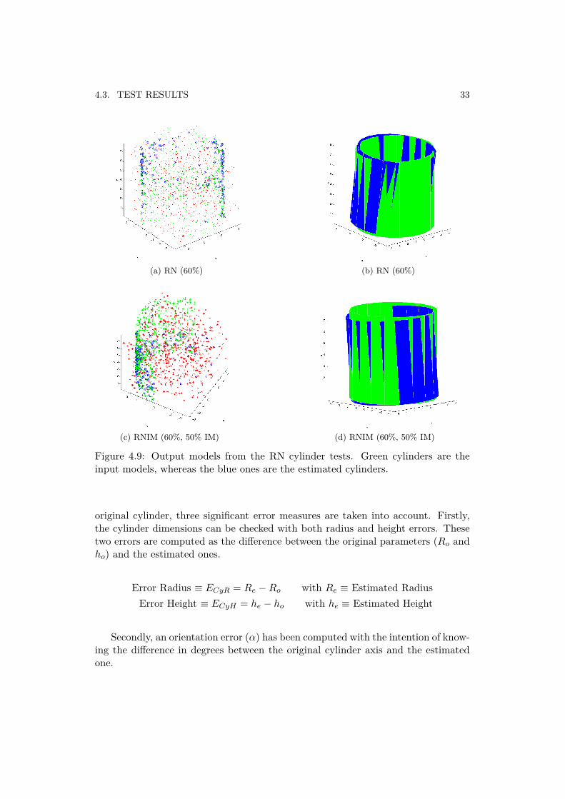
(a) RN (60%) (b) RN (60%)
(c) RNIM (60%, 50% IM) (d) RNIM (60%, 50% IM)
Figure 4.9: Output models from the RN cylinder tests. Green cylinders are theinput models, whereas the blue ones are the estimated cylinders.
original cylinder, three significant error measures are taken into account. Firstly,the cylinder dimensions can be checked with both radius and height errors. Thesetwo errors are computed as the difference between the original parameters (Ro andho) and the estimated ones.
Error Radius ≡ ECyR = Re −Ro with Re ≡ Estimated RadiusError Height ≡ ECyH = he − ho with he ≡ Estimated Height
Secondly, an orientation error (α) has been computed with the intention of know-ing the difference in degrees between the original cylinder axis and the estimatedone.
34 CHAPTER 4. EXPERIMENTAL EVALUATION
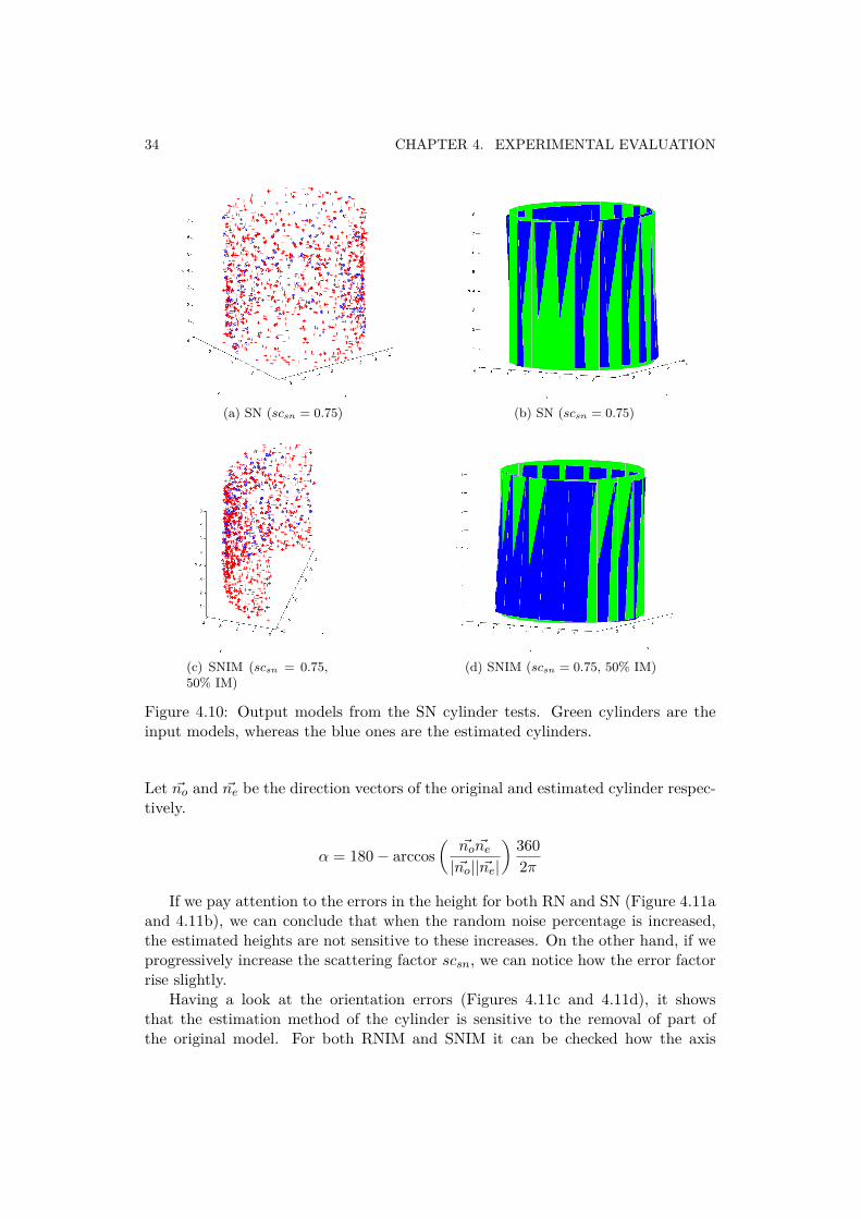
(a) SN (scsn = 0.75) (b) SN (scsn = 0.75)
(c) SNIM (scsn = 0.75,50% IM)
(d) SNIM (scsn = 0.75, 50% IM)
Figure 4.10: Output models from the SN cylinder tests. Green cylinders are theinput models, whereas the blue ones are the estimated cylinders.
Let ~no and ~ne be the direction vectors of the original and estimated cylinder respec-tively.
α = 180− arccos(~no ~ne| ~no|| ~ne|
) 3602π
If we pay attention to the errors in the height for both RN and SN (Figure 4.11aand 4.11b), we can conclude that when the random noise percentage is increased,the estimated heights are not sensitive to these increases. On the other hand, if weprogressively increase the scattering factor scsn, we can notice how the error factorrise slightly.
Having a look at the orientation errors (Figures 4.11c and 4.11d), it showsthat the estimation method of the cylinder is sensitive to the removal of part ofthe original model. For both RNIM and SNIM it can be checked how the axis
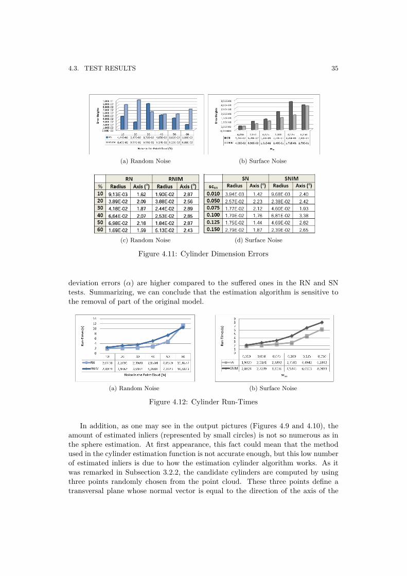
4.3. TEST RESULTS 35
(a) Random Noise (b) Surface Noise
(c) Random Noise (d) Surface Noise
Figure 4.11: Cylinder Dimension Errors
deviation errors (α) are higher compared to the suffered ones in the RN and SNtests. Summarizing, we can conclude that the estimation algorithm is sensitive tothe removal of part of the original model.
(a) Random Noise (b) Surface Noise
Figure 4.12: Cylinder Run-Times
In addition, as one may see in the output pictures (Figures 4.9 and 4.10), theamount of estimated inliers (represented by small circles) is not so numerous as inthe sphere estimation. At first appearance, this fact could mean that the methodused in the cylinder estimation function is not accurate enough, but this low numberof estimated inliers is due to how the estimation cylinder algorithm works. As itwas remarked in Subsection 3.2.2, the candidate cylinders are computed by usingthree points randomly chosen from the point cloud. These three points define atransversal plane whose normal vector is equal to the direction of the axis of the
36 CHAPTER 4. EXPERIMENTAL EVALUATION
cylinder. Since the points which define the primitive shape are randomly located onits surface, it is very unlikely to take three points exactly positioned on a transversalplane to the original cylinder. In spite of this fact, for the cylinder estimation, thenumber of estimated inliers is not so important. Insomuch, with a small set ofestimated inliers, a cylinder very similar to the original one can be reconstructed.
Paying attention to the runtimes graphs (Figure 4.12), we can check the time risecaused when noise conditions are increased. This did not happen in the case of ran-dom noise in the sphere evaluation, where the runtimes were held constant despiteincreasing the percentage of noise, because of the fact that the sphere algorithm isstronger to noise environments.
Conclusions RANSAC-Cylinder tests
The models obtained by the cylinder estimation algorithm are more sensitive tonoise when the model required to be estimated is incomplete. This is due to thefact that the set of points which defines the cylinder surface is smaller and thus,the noise points located in the region of the space where a part of the cylinder hasbeen removed may influence a deviation on the axis of this one.
Therefore, if the estimation of the axis suffers a small variation (with regardto the original one), the set of points will suffer it as well. Despite this fact, thealgorithm for computing the distances from points to an axis was finally chosenbecause of its good properties to rebuild cylindrical objects partially incomplete.
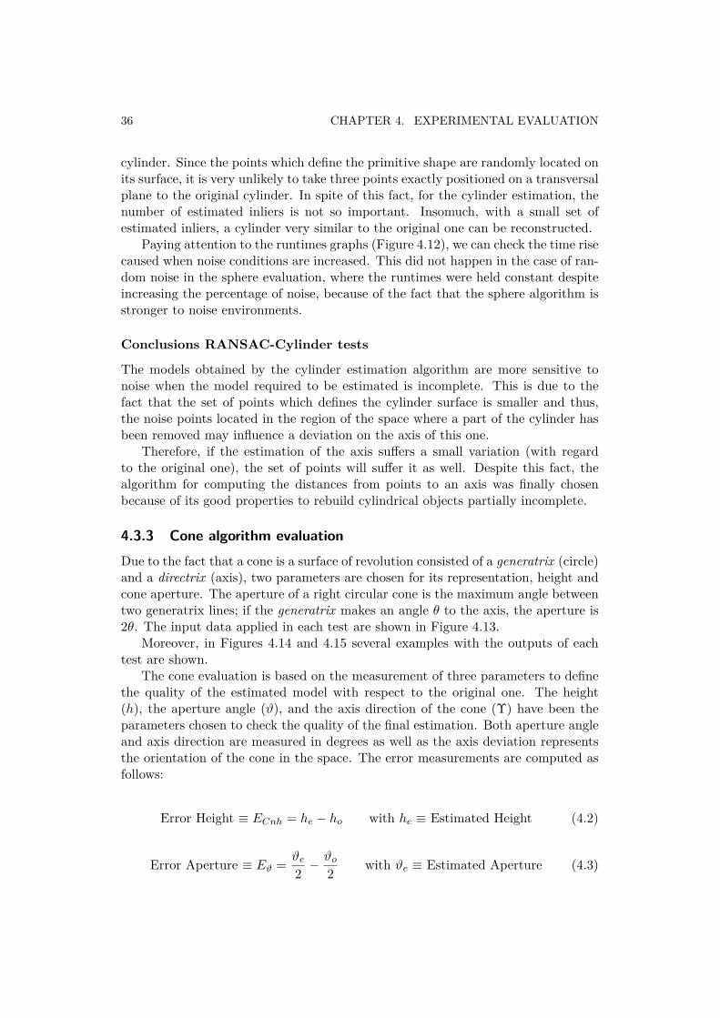
4.3.3 Cone algorithm evaluationDue to the fact that a cone is a surface of revolution consisted of a generatrix (circle)and a directrix (axis), two parameters are chosen for its representation, height andcone aperture. The aperture of a right circular cone is the maximum angle betweentwo generatrix lines; if the generatrix makes an angle θ to the axis, the aperture is2θ. The input data applied in each test are shown in Figure 4.13.
Moreover, in Figures 4.14 and 4.15 several examples with the outputs of eachtest are shown.
The cone evaluation is based on the measurement of three parameters to definethe quality of the estimated model with respect to the original one. The height(h), the aperture angle (ϑ), and the axis direction of the cone (Υ) have been theparameters chosen to check the quality of the final estimation. Both aperture angleand axis direction are measured in degrees as well as the axis deviation representsthe orientation of the cone in the space. The error measurements are computed asfollows:
Error Height ≡ ECnh = he − ho with he ≡ Estimated Height (4.2)
Error Aperture ≡ Eϑ = ϑe2− ϑo
2with ϑe ≡ Estimated Aperture (4.3)
4.3. TEST RESULTS 37
(a) RN (60%) (b) RNIM (60%, 50% IM)
(c) SN (scsn = 0.75) (d) SNIM (scsn = 0.75, 50%IM)
Figure 4.13: Cone Input models
To compute the correct cone orientation, the axis direction of the original cone hasbeen compared with the axis direction of the estimated cone.
Error Axis ≡ EΥ = Υe −Υo with Υe ≡ Estimated Axis (4.4)
In a similar way as was done for the cylinder, the height of the estimated cone iscomputed by projecting all the estimated inliers on the estimated cone axis. Once,all the points have been projected on the axis, the distance between those twopoints whose projections are more distant from each other will define the height ofthe estimated cone (Figure 3.6).
Regarding the height graphs (Figures 4.16a and 4.16b), we can observe as underthe same noise conditions, those tests where 50% of the original cone is deleted(RNIM and SNIM), the estimated cones have higher error values. Consequently,the estimations are more accurate when a greater amount of information about thesurface of the model is provided.
38 CHAPTER 4. EXPERIMENTAL EVALUATION
(a) RN (60%) (b) RN (60%)
(c) RNIM (60%, 50% IM) (d) RNIM (60%, 50% IM)
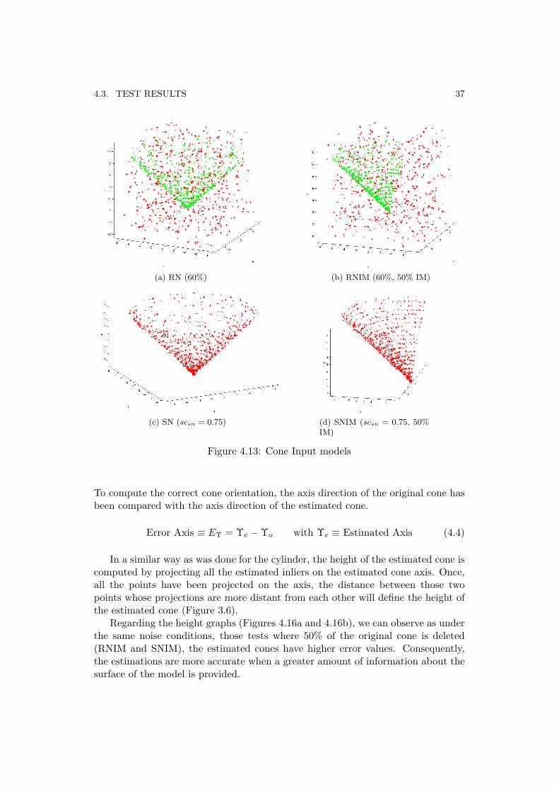
Figure 4.14: Output models from the RN cone tests. Green cones are the inputmodels, whereas the blue ones are the estimated cones.
Similarly, for the aperture and axis orientation errors (Figures 4.16c and 4.16d)we can find the same conclusions. Nevertheless, paying attention in these two mea-surements, we can realize that if the noise value is increased, the error measurementsdo not rise in the same way, but the errors keep constant around a central value.This fact indicates the strength of the estimation cone algorithm under differentnoise environments.
In Figure 4.17 the runtimes are very similar in the RN tests and SN tests. Thesevalues are much higher than the obtained for the sphere and cylinder because of thecomplexity of the estimation cone algorithm (Subsection 3.2.3). The rise in timecaused by increased noise is a consequence of the RANSAC algorithm. When thenoise conditions are significantly high, the algorithm is not capable of finding a set ofestimated inliers good enough which allows to leave the main loop (Subsection 3.1.1).Thereby, the estimation process will keep running until the maximum number ofiterations has been reached. This fact could hardly be appreciated in the sphere and
4.3. TEST RESULTS 39
(a) SN (scsn = 0.75) (b) SN (scsn = 0.75)
(c) SNIM (scsn = 0.75, 50% IM) (d) SNIM (scsn = 0.75, 50% IM)
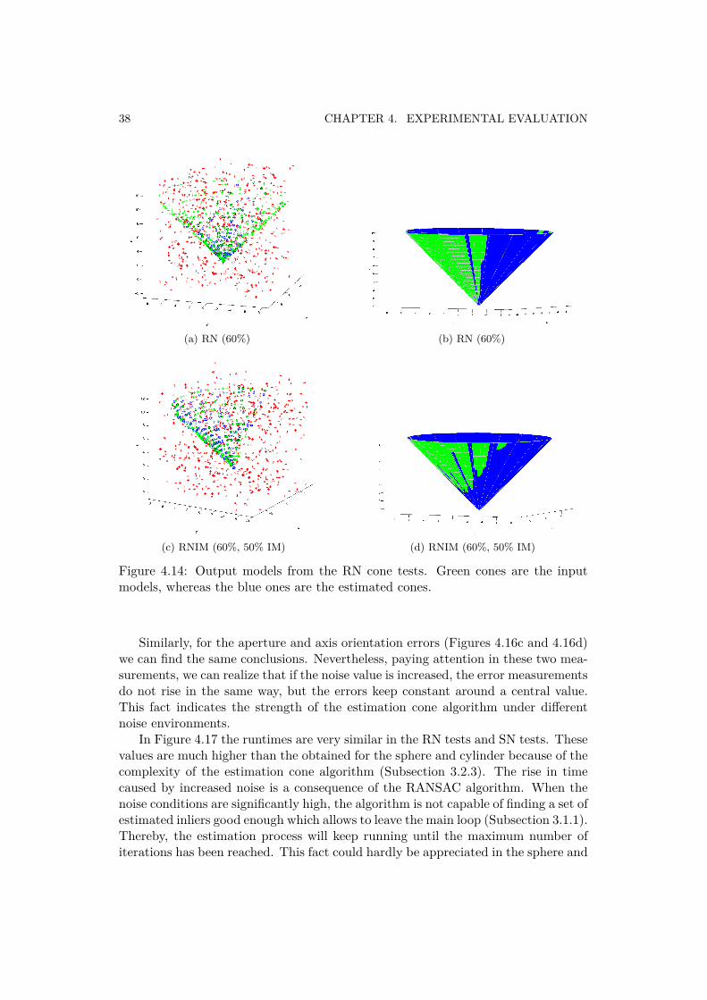
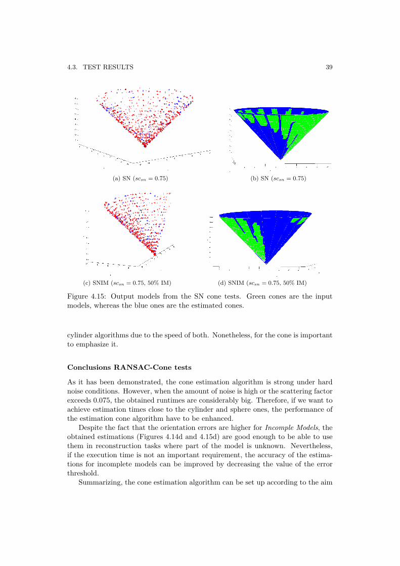
Figure 4.15: Output models from the SN cone tests. Green cones are the inputmodels, whereas the blue ones are the estimated cones.
cylinder algorithms due to the speed of both. Nonetheless, for the cone is importantto emphasize it.
Conclusions RANSAC-Cone tests
As it has been demonstrated, the cone estimation algorithm is strong under hardnoise conditions. However, when the amount of noise is high or the scattering factorexceeds 0.075, the obtained runtimes are considerably big. Therefore, if we want toachieve estimation times close to the cylinder and sphere ones, the performance ofthe estimation cone algorithm have to be enhanced.
Despite the fact that the orientation errors are higher for Incomple Models, theobtained estimations (Figures 4.14d and 4.15d) are good enough to be able to usethem in reconstruction tasks where part of the model is unknown. Nevertheless,if the execution time is not an important requirement, the accuracy of the estima-tions for incomplete models can be improved by decreasing the value of the errorthreshold.
Summarizing, the cone estimation algorithm can be set up according to the aim
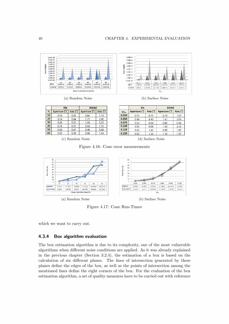
40 CHAPTER 4. EXPERIMENTAL EVALUATION
(a) Random Noise (b) Surface Noise
(c) Random Noise (d) Surface Noise
Figure 4.16: Cone error measurements
(a) Random Noise (b) Surface Noise
Figure 4.17: Cone Run-Times
which we want to carry out.
4.3.4 Box algorithm evaluation
The box estimation algorithm is due to its complexity, one of the most vulnerablealgorithms when different noise conditions are applied. As it was already explainedin the previous chapter (Section 3.2.4), the estimation of a box is based on thecalculation of six different planes. The lines of intersection generated by theseplanes define the edges of the box, as well as the points of intersection among thementioned lines define the eight corners of the box. For the evaluation of the boxestimation algorithm, a set of quality measures have to be carried out with reference
4.3. TEST RESULTS 41
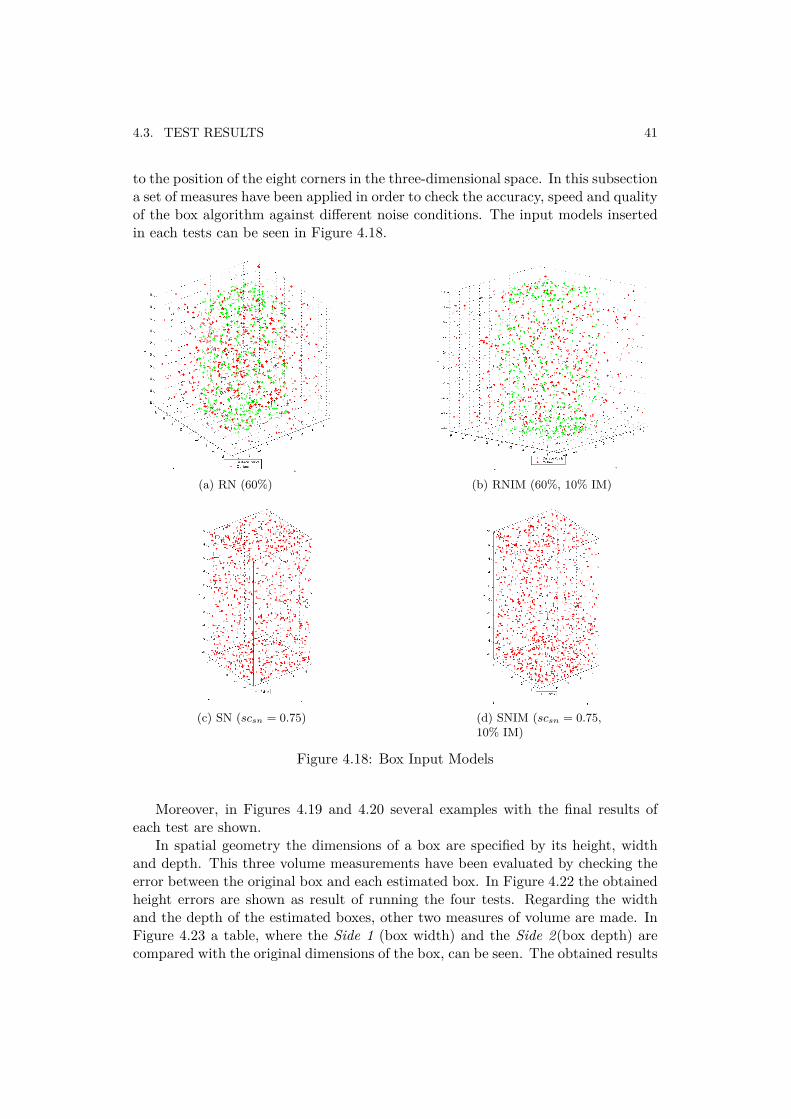
to the position of the eight corners in the three-dimensional space. In this subsectiona set of measures have been applied in order to check the accuracy, speed and qualityof the box algorithm against different noise conditions. The input models insertedin each tests can be seen in Figure 4.18.
(a) RN (60%) (b) RNIM (60%, 10% IM)
(c) SN (scsn = 0.75) (d) SNIM (scsn = 0.75,10% IM)
Figure 4.18: Box Input Models
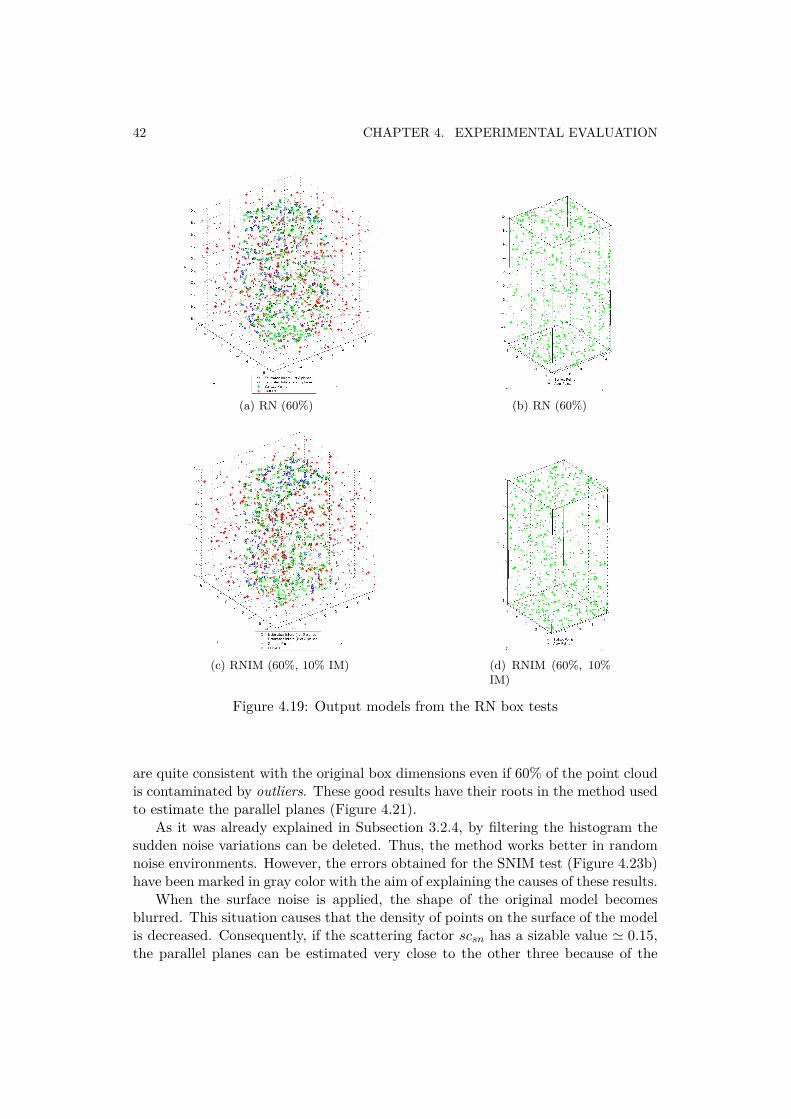
Moreover, in Figures 4.19 and 4.20 several examples with the final results ofeach test are shown.
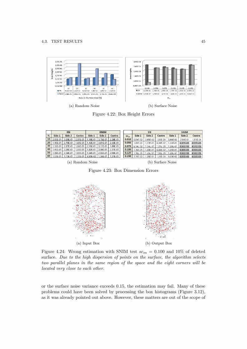
In spatial geometry the dimensions of a box are specified by its height, widthand depth. This three volume measurements have been evaluated by checking theerror between the original box and each estimated box. In Figure 4.22 the obtainedheight errors are shown as result of running the four tests. Regarding the widthand the depth of the estimated boxes, other two measures of volume are made. InFigure 4.23 a table, where the Side 1 (box width) and the Side 2(box depth) arecompared with the original dimensions of the box, can be seen. The obtained results
42 CHAPTER 4. EXPERIMENTAL EVALUATION
(a) RN (60%) (b) RN (60%)
(c) RNIM (60%, 10% IM) (d) RNIM (60%, 10%IM)
Figure 4.19: Output models from the RN box tests
are quite consistent with the original box dimensions even if 60% of the point cloudis contaminated by outliers. These good results have their roots in the method usedto estimate the parallel planes (Figure 4.21).
As it was already explained in Subsection 3.2.4, by filtering the histogram thesudden noise variations can be deleted. Thus, the method works better in randomnoise environments. However, the errors obtained for the SNIM test (Figure 4.23b)have been marked in gray color with the aim of explaining the causes of these results.
When the surface noise is applied, the shape of the original model becomesblurred. This situation causes that the density of points on the surface of the modelis decreased. Consequently, if the scattering factor scsn has a sizable value ' 0.15,the parallel planes can be estimated very close to the other three because of the
4.3. TEST RESULTS 43
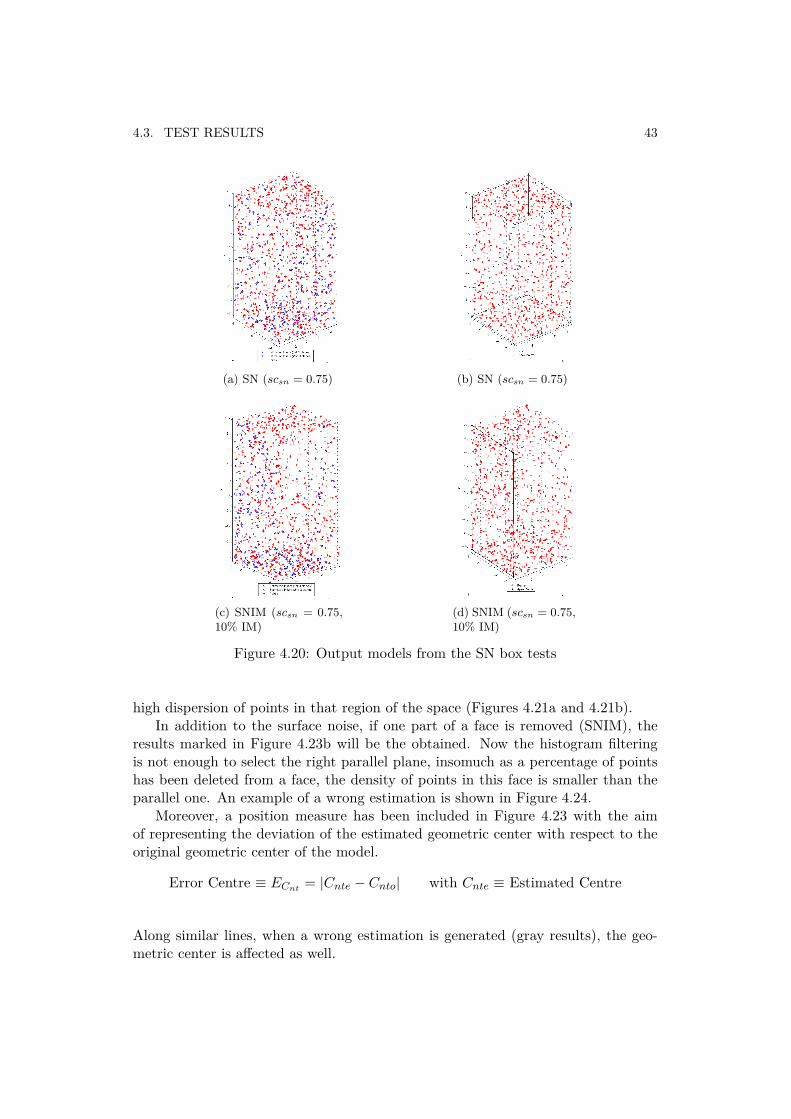
(a) SN (scsn = 0.75) (b) SN (scsn = 0.75)
(c) SNIM (scsn = 0.75,10% IM)
(d) SNIM (scsn = 0.75,10% IM)
Figure 4.20: Output models from the SN box tests
high dispersion of points in that region of the space (Figures 4.21a and 4.21b).In addition to the surface noise, if one part of a face is removed (SNIM), the
results marked in Figure 4.23b will be the obtained. Now the histogram filteringis not enough to select the right parallel plane, insomuch as a percentage of pointshas been deleted from a face, the density of points in this face is smaller than theparallel one. An example of a wrong estimation is shown in Figure 4.24.
Moreover, a position measure has been included in Figure 4.23 with the aimof representing the deviation of the estimated geometric center with respect to theoriginal geometric center of the model.
Error Centre ≡ ECnt = |Cnte − Cnto| with Cnte ≡ Estimated Centre
Along similar lines, when a wrong estimation is generated (gray results), the geo-metric center is affected as well.
44 CHAPTER 4. EXPERIMENTAL EVALUATION
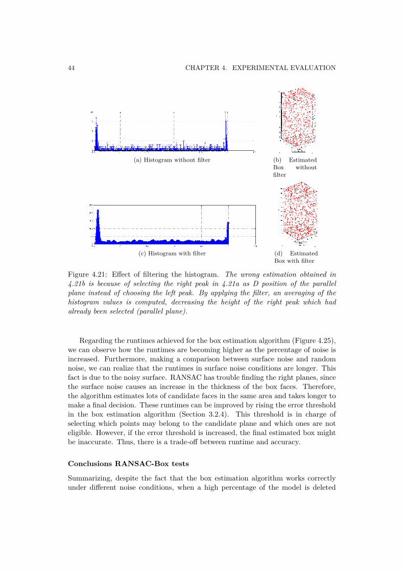
(a) Histogram without filter (b) EstimatedBox withoutfilter
(c) Histogram with filter (d) EstimatedBox with filter
Figure 4.21: Effect of filtering the histogram. The wrong estimation obtained in4.21b is because of selecting the right peak in 4.21a as D position of the parallelplane instead of choosing the left peak. By applying the filter, an averaging of thehistogram values is computed, decreasing the height of the right peak which hadalready been selected (parallel plane).
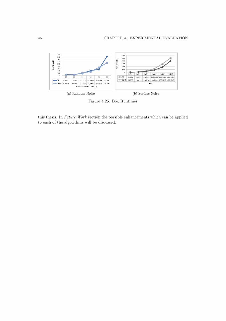
Regarding the runtimes achieved for the box estimation algorithm (Figure 4.25),we can observe how the runtimes are becoming higher as the percentage of noise isincreased. Furthermore, making a comparison between surface noise and randomnoise, we can realize that the runtimes in surface noise conditions are longer. Thisfact is due to the noisy surface. RANSAC has trouble finding the right planes, sincethe surface noise causes an increase in the thickness of the box faces. Therefore,the algorithm estimates lots of candidate faces in the same area and takes longer tomake a final decision. These runtimes can be improved by rising the error thresholdin the box estimation algorithm (Section 3.2.4). This threshold is in charge ofselecting which points may belong to the candidate plane and which ones are noteligible. However, if the error threshold is increased, the final estimated box mightbe inaccurate. Thus, there is a trade-off between runtime and accuracy.
Conclusions RANSAC-Box tests
Summarizing, despite the fact that the box estimation algorithm works correctlyunder different noise conditions, when a high percentage of the model is deleted
4.3. TEST RESULTS 45
(a) Random Noise (b) Surface Noise
Figure 4.22: Box Height Errors
(a) Random Noise (b) Surface Noise
Figure 4.23: Box Dimension Errors
(a) Input Box (b) Output Box
Figure 4.24: Wrong estimation with SNIM test scsn = 0.100 and 10% of deletedsurface. Due to the high dispersion of points on the surface, the algorithm selectstwo parallel planes in the same region of the space and the eight corners will belocated very close to each other.
or the surface noise variance exceeds 0.15, the estimation may fail. Many of theseproblems could have been solved by processing the box histograms (Figure 3.12),as it was already pointed out above. However, these matters are out of the scope of
46 CHAPTER 4. EXPERIMENTAL EVALUATION
(a) Random Noise (b) Surface Noise
Figure 4.25: Box Runtimes
this thesis. In Future Work section the possible enhancements which can be appliedto each of the algorithms will be discussed.
Chapter 5
Primitive Shape DecompositionAlgorithm
In this chapter, the algorithm that implements the decomposition of an object inseveral primitive shapes is going to be introduced. For this purpose, the RANSACcore algorithm, the primitive shape estimation algorithms and the BoxDecomposi-tion algorithm have been joined together in a single program called The PrimitiveShape Decomposition Algorithm (PSDA). In previous chapters the different partsthat configure the PSDA have been mentioned. However, the whole operation planis going to be discussed in this chapter.
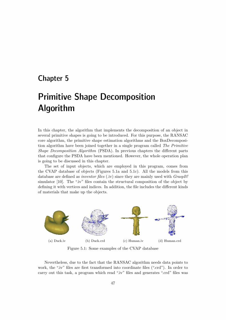
The set of input objects, which are employed in this program, comes fromthe CVAP database of objects (Figures 5.1a and 5.1c). All the models from thisdatabase are defined as inventor files (.iv) since they are mainly used with GraspIt!simulator [10]. The “.iv” files contain the structural composition of the object bydefining it with vertices and indices. In addition, the file includes the different kindsof materials that make up the objects.
(a) Duck.iv (b) Duck.crd (c) Human.iv (d) Human.crd
Figure 5.1: Some examples of the CVAP database
Nevertheless, due to the fact that the RANSAC algorithm needs data points towork, the “.iv” files are first transformed into coordinate files (“.crd”). In order tocarry out this task, a program which read “.iv” files and generates “.crd” files was
47
48 CHAPTER 5. PRIMITIVE SHAPE DECOMPOSITION ALGORITHM
designed. The “.crd” file contains the three-dimensional coordinates of the surfacepoints of a model (Figures 5.1b and 5.1d).
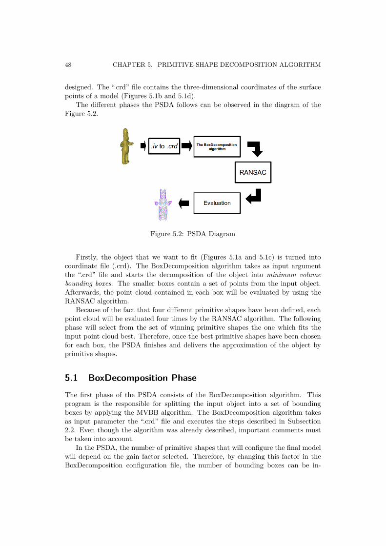
The different phases the PSDA follows can be observed in the diagram of theFigure 5.2.
Figure 5.2: PSDA Diagram
Firstly, the object that we want to fit (Figures 5.1a and 5.1c) is turned intocoordinate file (.crd). The BoxDecomposition algorithm takes as input argumentthe “.crd” file and starts the decomposition of the object into minimum volumebounding boxes. The smaller boxes contain a set of points from the input object.Afterwards, the point cloud contained in each box will be evaluated by using theRANSAC algorithm.
Because of the fact that four different primitive shapes have been defined, eachpoint cloud will be evaluated four times by the RANSAC algorithm. The followingphase will select from the set of winning primitive shapes the one which fits theinput point cloud best. Therefore, once the best primitive shapes have been chosenfor each box, the PSDA finishes and delivers the approximation of the object byprimitive shapes.
5.1 BoxDecomposition Phase
The first phase of the PSDA consists of the BoxDecomposition algorithm. Thisprogram is the responsible for splitting the input object into a set of boundingboxes by applying the MVBB algorithm. The BoxDecomposition algorithm takesas input parameter the “.crd” file and executes the steps described in Subsection2.2. Even though the algorithm was already described, important comments mustbe taken into account.
In the PSDA, the number of primitive shapes that will configure the final modelwill depend on the gain factor selected. Therefore, by changing this factor in theBoxDecomposition configuration file, the number of bounding boxes can be in-
5.2. RANSAC PHASE 49
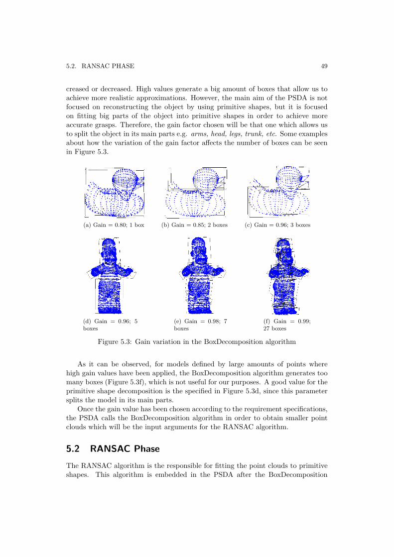
creased or decreased. High values generate a big amount of boxes that allow us toachieve more realistic approximations. However, the main aim of the PSDA is notfocused on reconstructing the object by using primitive shapes, but it is focusedon fitting big parts of the object into primitive shapes in order to achieve moreaccurate grasps. Therefore, the gain factor chosen will be that one which allows usto split the object in its main parts e.g. arms, head, legs, trunk, etc. Some examplesabout how the variation of the gain factor affects the number of boxes can be seenin Figure 5.3.
(a) Gain = 0.80; 1 box (b) Gain = 0.85; 2 boxes (c) Gain = 0.96; 3 boxes
(d) Gain = 0.96; 5boxes
(e) Gain = 0.98; 7boxes
(f) Gain = 0.99;27 boxes
Figure 5.3: Gain variation in the BoxDecomposition algorithm
As it can be observed, for models defined by large amounts of points wherehigh gain values have been applied, the BoxDecomposition algorithm generates toomany boxes (Figure 5.3f), which is not useful for our purposes. A good value for theprimitive shape decomposition is the specified in Figure 5.3d, since this parametersplits the model in its main parts.
Once the gain value has been chosen according to the requirement specifications,the PSDA calls the BoxDecomposition algorithm in order to obtain smaller pointclouds which will be the input arguments for the RANSAC algorithm.
5.2 RANSAC PhaseThe RANSAC algorithm is the responsible for fitting the point clouds to primitiveshapes. This algorithm is embedded in the PSDA after the BoxDecomposition
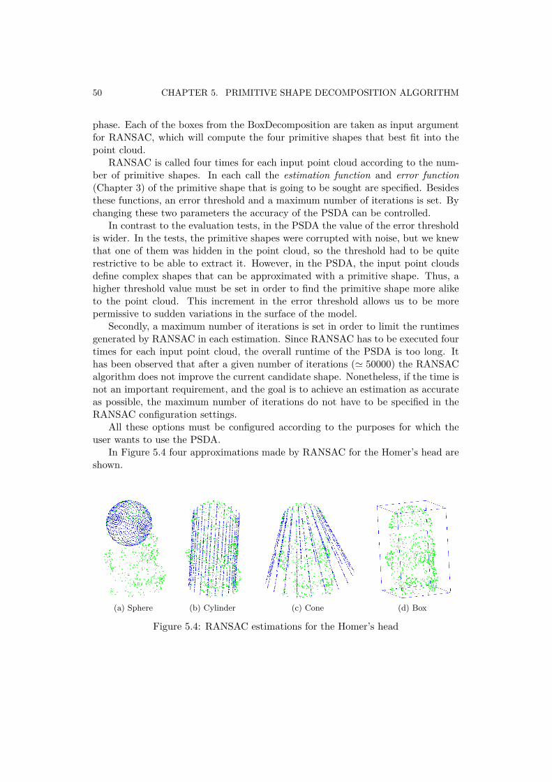
50 CHAPTER 5. PRIMITIVE SHAPE DECOMPOSITION ALGORITHM
phase. Each of the boxes from the BoxDecomposition are taken as input argumentfor RANSAC, which will compute the four primitive shapes that best fit into thepoint cloud.
RANSAC is called four times for each input point cloud according to the num-ber of primitive shapes. In each call the estimation function and error function(Chapter 3) of the primitive shape that is going to be sought are specified. Besidesthese functions, an error threshold and a maximum number of iterations is set. Bychanging these two parameters the accuracy of the PSDA can be controlled.
In contrast to the evaluation tests, in the PSDA the value of the error thresholdis wider. In the tests, the primitive shapes were corrupted with noise, but we knewthat one of them was hidden in the point cloud, so the threshold had to be quiterestrictive to be able to extract it. However, in the PSDA, the input point cloudsdefine complex shapes that can be approximated with a primitive shape. Thus, ahigher threshold value must be set in order to find the primitive shape more aliketo the point cloud. This increment in the error threshold allows us to be morepermissive to sudden variations in the surface of the model.
Secondly, a maximum number of iterations is set in order to limit the runtimesgenerated by RANSAC in each estimation. Since RANSAC has to be executed fourtimes for each input point cloud, the overall runtime of the PSDA is too long. Ithas been observed that after a given number of iterations (' 50000) the RANSACalgorithm does not improve the current candidate shape. Nonetheless, if the time isnot an important requirement, and the goal is to achieve an estimation as accurateas possible, the maximum number of iterations do not have to be specified in theRANSAC configuration settings.
All these options must be configured according to the purposes for which theuser wants to use the PSDA.
In Figure 5.4 four approximations made by RANSAC for the Homer’s head areshown.
(a) Sphere (b) Cylinder (c) Cone (d) Box
Figure 5.4: RANSAC estimations for the Homer’s head
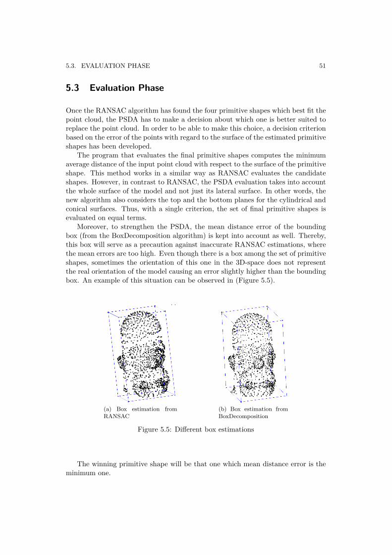
5.3. EVALUATION PHASE 51
5.3 Evaluation Phase
Once the RANSAC algorithm has found the four primitive shapes which best fit thepoint cloud, the PSDA has to make a decision about which one is better suited toreplace the point cloud. In order to be able to make this choice, a decision criterionbased on the error of the points with regard to the surface of the estimated primitiveshapes has been developed.
The program that evaluates the final primitive shapes computes the minimumaverage distance of the input point cloud with respect to the surface of the primitiveshape. This method works in a similar way as RANSAC evaluates the candidateshapes. However, in contrast to RANSAC, the PSDA evaluation takes into accountthe whole surface of the model and not just its lateral surface. In other words, thenew algorithm also considers the top and the bottom planes for the cylindrical andconical surfaces. Thus, with a single criterion, the set of final primitive shapes isevaluated on equal terms.
Moreover, to strengthen the PSDA, the mean distance error of the boundingbox (from the BoxDecomposition algorithm) is kept into account as well. Thereby,this box will serve as a precaution against inaccurate RANSAC estimations, wherethe mean errors are too high. Even though there is a box among the set of primitiveshapes, sometimes the orientation of this one in the 3D-space does not representthe real orientation of the model causing an error slightly higher than the boundingbox. An example of this situation can be observed in (Figure 5.5).
(a) Box estimation fromRANSAC
(b) Box estimation fromBoxDecomposition
Figure 5.5: Different box estimations
The winning primitive shape will be that one which mean distance error is theminimum one.
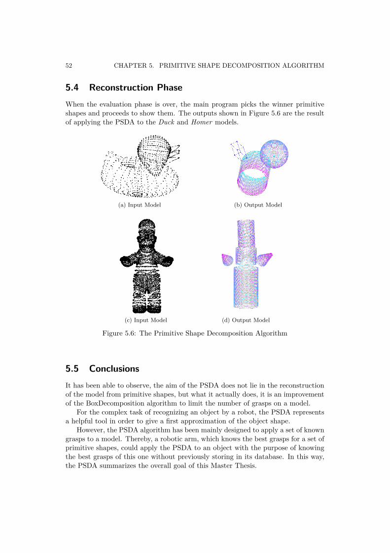
52 CHAPTER 5. PRIMITIVE SHAPE DECOMPOSITION ALGORITHM
5.4 Reconstruction PhaseWhen the evaluation phase is over, the main program picks the winner primitiveshapes and proceeds to show them. The outputs shown in Figure 5.6 are the resultof applying the PSDA to the Duck and Homer models.
(a) Input Model (b) Output Model
(c) Input Model (d) Output Model
Figure 5.6: The Primitive Shape Decomposition Algorithm
5.5 ConclusionsIt has been able to observe, the aim of the PSDA does not lie in the reconstructionof the model from primitive shapes, but what it actually does, it is an improvementof the BoxDecomposition algorithm to limit the number of grasps on a model.
For the complex task of recognizing an object by a robot, the PSDA representsa helpful tool in order to give a first approximation of the object shape.
However, the PSDA algorithm has been mainly designed to apply a set of knowngrasps to a model. Thereby, a robotic arm, which knows the best grasps for a set ofprimitive shapes, could apply the PSDA to an object with the purpose of knowingthe best grasps of this one without previously storing in its database. In this way,the PSDA summarizes the overall goal of this Master Thesis.
Chapter 6
Conclusion and Future Work
6.1 Conclusion
At the beginning of this thesis, a method that tries to solve the problem of findingsuitable graps for unknown objects was proposed. To be able to carry out this task,a program capable of implementing all the proposed goals was created. The PSDAmakes an attempt to integrate several algorithm into one, with the final purpose ofbeing embedded into robotic machines.
The present Master Thesis may be structured in two parts. First, four estima-tion algorithms have been designed to extract primitive shapes from data points.The algorithms are based on RANSAC, which is the base platform to run these es-timation programs. Second, the PSDA represents an algorithm that takes as inputdata the results obtained from the BoxDecomposition and applies the RANSACalgorithm.
In the evaluation chapter (Chapter 4), the quality of each of the estimationalgorithms was evaluated by applying four kind of noise scenarios. The resultsobtained in the tests have allowed us to realize that these estimation algorithmscan be used in reconstruction tasks where the reconstructed point clouds are notwell defined.
Finally, the PSDA tries to coordinate all the algorithms. Even though this finalalgorithm works quite well, there are many parts that still have to be improved.Thereby, some of these improvements will be mentioned in the Future Work sectionwith the purpose of optimizing the speed and the reliability of the algorithm.
6.2 Future Work
In the RANSAC algorithm, a pre-filter phase would have to be incorporated inorder to reduce the amount of possible candidate estimations. Thus, all thoseiterations where the estimated shapes are too big or too small would be rejected,causing an essential enhancement in the RANSAC runtimes. Moreover, insteadof having a fixed error threshold from the beginning of the program, an threshold
53
54 CHAPTER 6. CONCLUSION AND FUTURE WORK
value that varies according to the size of the candidate shape would produce moreaccurate results. However, since the core of the RANSAC algorithm was alreadyimplemented in Matlab, we did not want to modify this part of the program butsolely the estimation algorithms which describe the primitive shapes. Therefore, fora future implementation of this RANSAC version, all these issues have to be keptin mind.
Regarding the PSDA, maybe, the BoxDecomposition is not the best algorithmto split point clouds. This algorithm is based on MVBB and does not take intoaccount the size of the model. Consequently, sometimes the BoxDecompositiongenerates results as seen in Figures 5.3e and 5.3f, where the Homer’s feet are groupedtogether into the same minimum bounding box. This situation produces that theRANSAC algorithm fits only one foot instead of creating a primitive shape withboth feet. One possible solution to the problem might be that RANSAC searchesfor several primitive shapes in the same point cloud. But then, how many primitiveshapes should be searched in the same point cloud?, Would this solution increasesignificantly the overall runtime? Therefore, as can be thought, the PSDA is acomplex algorithm that must be examined carefully.
References
[1] The PACO-PLUS Project. URL: http://www.paco-plus.org/, November2006.
[2] The RANSAC toolbox for Matlab. URL:"http://vision.ece.ucsb.edu/ zuliani",November 2006.
[3] Gill Barequet and Sariel Har-Peled. Efficiently approximating the minimum-volume bounding box of a point set in three dimensions. J. Algorithms,38(1):91–109, 2001.
[4] Paul J. Besl and Neil D. Mckay. A method for registration of 3-d shapes.IEEE Transactions on Pattern Analysis and Machine Intelligence, 14(2):239–256, February 1992.
[5] Ondrej Chum and Jiri Matas. Matching with prosac - progressive sampleconsensus. In CVPR ’05: Proceedings of the 2005 IEEE Computer SocietyConference on Computer Vision and Pattern Recognition (CVPR’05) - Volume1, pages 220–226, Washington, DC, USA, 2005. IEEE Computer Society.
[6] J. Bohg et al. Applying shape context in robotic grasping.URL:"http://www.csc.kth.se/ bohg", 2009.
[7] Martin A. Fischler and Robert C. Bolles. Random sample consensus: aparadigm for model fitting with applications to image analysis and automatedcartography. pages 726–740, 1987.
[8] K. Huebner, S. Ruthotto, and D. Kragic. Minimum volume bounding box de-composition for shape approximation in robot grasping. In IEEE InternationalConference on Robotics and Automation, 2008., pages 1628–1633, 2008.
[9] A. T. Miller, S. Knoop, H. Christensen, and P. K. Allen. Automatic graspplanning using shape primitives. In Proceedings of the IEEE InternationalConference on Robotics and Automation, 2003, volume 2, pages 1824–1829,2003.
[10] Andrew Tesch Miller. Graspit!: a versatile simulator for robotic grasping. PhDthesis, New York, NY, USA, 2001. Adviser-Allen, Peter K.
55
56 REFERENCES
[11] Szymon Rusinkiewicz and Marc Levoy. Efficient variants of the icp algorithm.In Proceedings of the Third Intl. Conf. on 3D Digital Imaging and Modeling,pages 145–152, 2001.
[12] Ruwen Schnabel, Patrick Degener, and Reinhard Klein. Completion and re-construction with primitive shapes. Computer Graphics Forum, 28(2):503–512.
[13] Ruwen Schnabel, Roland Wahl, and Reinhard Klein. Efficient ransac for point-cloud shape detection. Computer Graphics Forum, 26(2):214–226, June 2007.
[14] Ben J. Tordoff. Guided-mlesac: Faster image transform estimation by usingmatching priors. IEEE Trans. Pattern Anal. Mach. Intell., 27(10):1523–1535,2005. Member-Murray, David W.
[15] P. H. S. Torr and A. Zisserman. Mlesac: a new robust estimator with applica-tion to estimating image geometry. Comput. Vis. Image Underst., 78(1):138–156, 2000.
[16] Marco Zuliani. RANSAC for Dummies. MathWorks,URL:"http://www.mathworks.com", November 2008.

TRITA-CSC-E 2009:131 ISRN-KTH/CSC/E--09/131--SE
ISSN-1653-5715
www.kth.se