Embed Size (px)
Citation preview

Panel Data Linear Models
Fitting Panel Data Linear Models in Stata
Gustavo Sanchez
Senior StatisticianStataCorp LP
Puebla, Mexico
Gustavo Sanchez (StataCorp) June 22-23, 2012 1 / 42
Panel Data Linear Models
Outline
Outline
Brief introduction to panel data linear models
Fixed and Random effects models
Fitting the model in Stata
Specifying the panel structure
Regression output
Testing and accounting for serial correlation andheteroskedasticity
Panel Unit root tests - Model in first differences
Dynamic panel linear models
Gustavo Sanchez (StataCorp) June 22-23, 2012 2 / 42

Panel Data Linear Models
Introduction to Panel Data Linear Models
Brief Introduction to Panel Data Linear Models
Gustavo Sanchez (StataCorp) June 22-23, 2012 3 / 42

Panel Data Linear Models
Introduction to Panel Data Linear Models
One-way error component model
One-way error component model
Yit = α + X 1it ∗ β1 + ... + XK
it ∗ βK + εit
Yit = α + X 1it ∗ β1 + ... + XK
it ∗ βK + µi + νit
i = 1, ...,N
j = 1, ...,T
Gustavo Sanchez (StataCorp) June 22-23, 2012 4 / 42

Panel Data Linear Models
Introduction to Panel Data Linear Models
One-way error component model - Fixed effects
Fixed Effects Models
Yit = α + X 1it ∗ β1 + ...+ XK
it ∗ βK + µi + νit
Some Relevant Assumptions
The non-observable individual effects are represented byfixed parameters
The explanatory variables in X are independent of theidiosyncratic error term but they are not independent ofthe individual fixed effects
The idiosyncratic error term νit is iid(0, σ2ν)
Gustavo Sanchez (StataCorp) June 22-23, 2012 5 / 42

Panel Data Linear Models
Introduction to Panel Data Linear Models
One-way error component model - Fixed effects
Fixed Effects Models
Let’s assume that we have only one explanatory variable:
Yit = α + Xit ∗ β + µi + νit
Let’s take the average in time:
Yi . = α + Xi . ∗ β + µi + νi .
Let’s take the difference between those two equations:
Yit − Yi . = (Xit − Xi .) ∗ β + (νit − νi .)
This ”within transformation” is the basis for the fixed effectsestimator.
The FE beta estimates could be obtained by using OLS in thelatest equation
Gustavo Sanchez (StataCorp) June 22-23, 2012 6 / 42

Panel Data Linear Models
Introduction to Panel Data Linear Models
One-way error component model - Random effects
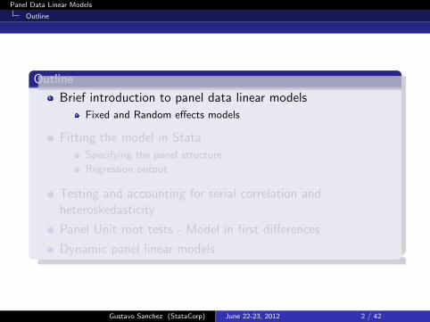
Random Effects Models
Yit = α + X 1it ∗ β1 + ...+ XK
it ∗ βK + µi + νit
Some Relevant Assumptions
The non-observable individual effects are iid(0,σ2µ)
The explanatory variables in X are independent of theidiosyncratic error term and they are also independent ofthe individual random effects (i.e. Cov(Xk
it , µi ) = 0)
The idiosyncratic error term νit is iid(0, σ2ν)
Gustavo Sanchez (StataCorp) June 22-23, 2012 7 / 42
Panel Data Linear Models
Introduction to Panel Data Linear Models
One-way error component model - Random effects
Random Effects Models
Yit = α + X 1it ∗ β1 + ...+ XK
it ∗ βK + µi + νit
Some Relevant Assumptions
The non-observable individual effects are iid(0,σ2µ)
The explanatory variables in X are independent of theidiosyncratic error term and they are also independent ofthe individual random effects (i.e. Cov(Xk
it , µi ) = 0)
The idiosyncratic error term νit is iid(0, σ2ν)
Gustavo Sanchez (StataCorp) June 22-23, 2012 7 / 42

Panel Data Linear Models
Fitting the model in Stata
Fitting the model in Stata
Gustavo Sanchez (StataCorp) June 22-23, 2012 8 / 42

Panel Data Linear Models
Fitting the model in Stata
Empirical example
Model for aggregate consumption
consumoit = α+pibit ∗β1 +pibit−1 ∗β2 + irateit ∗β3 +µi + νit
Data
World Bank public online data on:
consumo: Final consumption expenditure (Y2000=100)pib: Gross domestic product (Y2000=100)irate deposit interest rate
Example 1: 1980-2010 for 122 countries
Example 2: 2003-2010 for 104-108 countries :Source:http://databank.worldbank.org/data/Home.aspx
Gustavo Sanchez (StataCorp) June 22-23, 2012 9 / 42
Panel Data Linear Models
Fitting the model in Stata
Empirical example - Specifying the panel structure in Stata
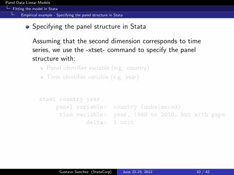
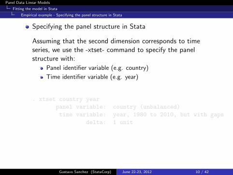
Specifying the panel structure in Stata
Assuming that the second dimension corresponds to timeseries, we use the -xtset- command to specify the panelstructure with:
Panel identifier variable (e.g. country)
Time identifier variable (e.g. year)
. xtset country year
panel variable: country (unbalanced)
time variable: year, 1980 to 2010, but with gaps
delta: 1 unit
Gustavo Sanchez (StataCorp) June 22-23, 2012 10 / 42
Panel Data Linear Models
Fitting the model in Stata
Empirical example - Specifying the panel structure in Stata
Specifying the panel structure in Stata
Assuming that the second dimension corresponds to timeseries, we use the -xtset- command to specify the panelstructure with:
Panel identifier variable (e.g. country)
Time identifier variable (e.g. year)
. xtset country year
panel variable: country (unbalanced)
time variable: year, 1980 to 2010, but with gaps
delta: 1 unit
Gustavo Sanchez (StataCorp) June 22-23, 2012 10 / 42

Panel Data Linear Models
Fitting the model in Stata
Empirical example - Fixed effects
Fixed effects linear model
. xtreg lconsumo lpib lirate,fe
Fixed-effects (within) regression Number of obs = 2901Group variable: country Number of groups = 122
R-sq: within = 0.9368 Obs per group: min = 11between = 0.9943 avg = 23.8overall = 0.9929 max = 31
F(2,2777) = 20586.83corr(u_i, Xb) = 0.3537 Prob > F = 0.0000
lconsumo Coef. Std. Err. t P>|t| [95% Conf. Interval]
lpib .9399169 .0052705 178.34 0.000 .9295824 .9502514lirate -.0041257 .002125 -1.94 0.052 -.0082925 .000041_cons 1.218756 .1274414 9.56 0.000 .9688669 1.468646
sigma_u .16078074sigma_e .07814221
rho .80892226 (fraction of variance due to u_i)
F test that all u_i=0: F(121, 2777) = 93.89 Prob > F = 0.0000
Gustavo Sanchez (StataCorp) June 22-23, 2012 11 / 42

Panel Data Linear Models
Testing and accounting for serial correlation and heteroskedasticity
Testing and accounting for serial correlation andheteroskedasticity
http://www.stata.com/support/faqs/stat/panel.html
Gustavo Sanchez (StataCorp) June 22-23, 2012 12 / 42

Panel Data Linear Models
Testing and accounting for serial correlation and heteroskedasticity
Empirical example - Test for autocorrelation
Test for autocorrelation: Wooldridge (2002, pag. 2823)derives a simple test for autocorrelation in panel-data models.
Regress the pooled (OLS) model in first difference and predictthe residualsRegress the residuals on its first lag and test the coefficient onthose lagged residuals
Drukker (2003) implements the test with the user-writtencommand -xtserial-
. xtserial lconsumo lpib lirate if e(sample)
Wooldridge test for autocorrelation in panel dataH0: no first-order autocorrelation
F( 1, 121) = 103.854Prob > F = 0.0000
Gustavo Sanchez (StataCorp) June 22-23, 2012 13 / 42

Panel Data Linear Models
Testing and accounting for serial correlation and heteroskedasticity
Empirical example - Test for heteroskedasticity
Test for heteroskedasticity: Poi and Wiggins (2001) suggestan LR test for panel-level heteroskedasticity:
iterated GLS with heteroskedastic panels produces MLE.
Thus, we can use a LR test with-xtgls, igls panels(heteroskdastic)- versus -xtgls, igls-
. quietly xtgls lconsumo lpib lirate, panels(heterosk) igls
. estimates store hetero
. quietly xtgls lconsumo lpib lirate, igls
. estimates store homosk
. local df = e(N_g) - 1
.
. lrtest hetero homosk , df(`df´)
Likelihood-ratio test LR chi2(121)= 3428.91(Assumption: homosk nested in hetero) Prob > chi2 = 0.0000
Gustavo Sanchez (StataCorp) June 22-23, 2012 14 / 42

Panel Data Linear Models
Testing and accounting for serial correlation and heteroskedasticity
One-way linear AR(1) model
Linear model with first order autoregressive error term-xtregar-:
Yit = α + X 1it ∗ β1 + ...+ XK
it ∗ βK + µi + νit
νit = ρ ∗ νit−1 + ηit ; η is iid(0, σ2η)
Some Relevant Assumptions
Fixed effects: The non-observable individual effects (µi )are represented by fixed parameters and may be correlatedwith the covariates in X.Random effects: The non-observable individual effects areassumed to be independent of the idiosyncratic error term andthey are also independent of the covariates in X. The µi
are iid(0,σ2µ)
Gustavo Sanchez (StataCorp) June 22-23, 2012 15 / 42

Panel Data Linear Models
Testing and accounting for serial correlation and heteroskedasticity
Empirical example - Fixed effects AR(1) model
Fit model accounting for autocorrelation
. xtregar lconsumo lpib lirate, fe
FE (within) regression with AR(1) disturbances Number of obs = 2779Group variable: country Number of groups = 122
R-sq: within = 0.9631 Obs per group: min = 10between = 0.9941 avg = 22.8overall = 0.9930 max = 30
F(2,2655) = 34634.76corr(u_i, Xb) = -0.2531 Prob > F = 0.0000
lconsumo Coef. Std. Err. t P>|t| [95% Conf. Interval]
lpib .9887413 .0037579 263.11 0.000 .9813726 .99611lirate -.000825 .0021888 -0.38 0.706 -.0051168 .0034668_cons .0431147 .015465 2.79 0.005 .01279 .0734394
rho_ar .82953965sigma_u .15647357sigma_e .04443063rho_fov .92538831 (fraction of variance because of u_i)
F test that all u_i=0: F(121,2655) = 9.24 Prob > F = 0.0000
Gustavo Sanchez (StataCorp) June 22-23, 2012 16 / 42
Panel Data Linear Models
Testing and accounting for serial correlation and heteroskedasticity
Feasible Generalized Least Squares (FGLS)
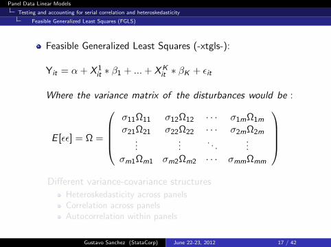
Feasible Generalized Least Squares (-xtgls-):
Yit = α + X 1it ∗ β1 + ...+ XK
it ∗ βK + εit
Where the variance matrix of the disturbances would be :
E [εε] = Ω =
σ11Ω11 σ12Ω12 · · · σ1mΩ1m
σ21Ω21 σ22Ω22 · · · σ2mΩ2m...
.... . .
...σm1Ωm1 σm2Ωm2 · · · σmmΩmm
Different variance-covariance structures
Heteroskedasticity across panelsCorrelation across panelsAutocorrelation within panels
Gustavo Sanchez (StataCorp) June 22-23, 2012 17 / 42

Panel Data Linear Models
Testing and accounting for serial correlation and heteroskedasticity
Feasible Generalized Least Squares (FGLS)
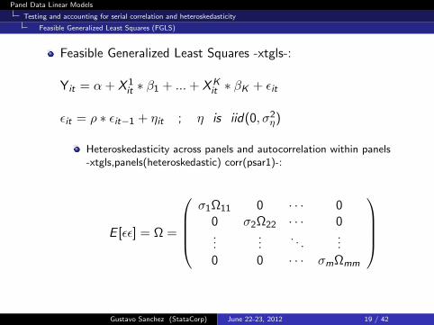
Feasible Generalized Least Squares -xtgls-:
Yit = α + X 1it ∗ β1 + ...+ XK
it ∗ βK + εit
Heteroskedasticity across panels -xtgls,panels(heteroskedastic)-:
E [εε] = Ω =
σ1I 0 · · · 00 σ2I · · · 0...
.... . .
...0 0 · · · σmI
Gustavo Sanchez (StataCorp) June 22-23, 2012 18 / 42
Panel Data Linear Models
Testing and accounting for serial correlation and heteroskedasticity
Feasible Generalized Least Squares (FGLS)
Feasible Generalized Least Squares -xtgls-:
Yit = α + X 1it ∗ β1 + ...+ XK
it ∗ βK + εit
εit = ρ ∗ εit−1 + ηit ; η is iid(0, σ2η)
Heteroskedasticity across panels and autocorrelation within panels-xtgls,panels(heteroskedastic) corr(psar1)-:
E [εε] = Ω =
σ1Ω11 0 · · · 0
0 σ2Ω22 · · · 0...
.... . .
...0 0 · · · σmΩmm
Gustavo Sanchez (StataCorp) June 22-23, 2012 19 / 42

Panel Data Linear Models
Testing and accounting for serial correlation and heteroskedasticity
Empirical example - Fit model accounting for heteroskedasticity
Fit model accounting for heteroskedasticity
. xtgls lconsumo lpib lirate,panels(heterosk) nolog
Cross-sectional time-series FGLS regression
Coefficients: generalized least squaresPanels: heteroskedasticCorrelation: no autocorrelation
Estimated covariances = 122 Number of obs = 2901Estimated autocorrelations = 0 Number of groups = 122Estimated coefficients = 3 Obs per group: min = 11
avg = 23.77869max = 31
Wald chi2(2) = 1352635Prob > chi2 = 0.0000
lconsumo Coef. Std. Err. z P>|z| [95% Conf. Interval]
lpib .9720376 .000853 1139.53 0.000 .9703657 .9737094lirate .0193624 .0013921 13.91 0.000 .016634 .0220908_cons .4192768 .0215707 19.44 0.000 .376999 .4615545
.
Gustavo Sanchez (StataCorp) June 22-23, 2012 20 / 42

Panel Data Linear Models
Testing and accounting for serial correlation and heteroskedasticity
Empirical example - Fit model accounting for autocorrelation and heteroskedasticity
Fit model accounting for autocorrelation andheteroskedasticity
. xtgls lconsumo lpib lirate,panels(heterosk) corr(psar1) nolog force
Cross-sectional time-series FGLS regression
Coefficients: generalized least squaresPanels: heteroskedasticCorrelation: panel-specific AR(1)
Estimated covariances = 122 Number of obs = 2901Estimated autocorrelations = 122 Number of groups = 122Estimated coefficients = 3 Obs per group: min = 11
avg = 23.77869max = 31
Wald chi2(2) = 255484.88Prob > chi2 = 0.0000
lconsumo Coef. Std. Err. z P>|z| [95% Conf. Interval]
lpib .957914 .0019214 498.54 0.000 .9541481 .96168lirate -.0009035 .0009393 -0.96 0.336 -.0027444 .0009375_cons .7854506 .0472898 16.61 0.000 .6927643 .8781369
.
Gustavo Sanchez (StataCorp) June 22-23, 2012 21 / 42
Panel Data Linear Models
Panel unit root tests - Model in first differences
Panel unit root tests - Model in first differences
Gustavo Sanchez (StataCorp) June 22-23, 2012 22 / 42

Panel Data Linear Models
Panel unit root tests - Model in first differences
Empirical example - Plot variables in log-levels
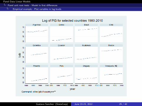
Command lines to plot the the variables in levels (per panel)
. xtline lconsumo if country==9 | country==25 | country==28 ///> | country==42 | country==44 | country==61 | country==87 ///> | country==146 | country==176 | country==179 | country==238 ///> | country==241, name(lconsumo) ///> byopts(t1title("Log of Consumo for selected countries 1980-2010") ///> note("Command: xtline lconsumo if country==**,[options]"))
.
Gustavo Sanchez (StataCorp) June 22-23, 2012 23 / 42

Panel Data Linear Models
Panel unit root tests - Model in first differences
Empirical example - Plot variables in log-levels
Gustavo Sanchez (StataCorp) June 22-23, 2012 24 / 42
Panel Data Linear Models
Panel unit root tests - Model in first differences
Empirical example - Plot variables in log-levels
Gustavo Sanchez (StataCorp) June 22-23, 2012 25 / 42

Panel Data Linear Models
Panel unit root tests - Model in first differences
Empirical example - Plot variables in log-levels
Gustavo Sanchez (StataCorp) June 22-23, 2012 26 / 42

Panel Data Linear Models
Panel unit root tests - Model in first differences
Panel unit root - Fisher-type test
Fisher-type Test (xtunitroot fisher)
Ho: All the panels have unit rootsH1: At least one panel does not have unit roots (N finite),or some panels do not have unit roots (N →∞)
Allows unbalanced panels and gaps in any panel
Performs Dickey-Fuller or Phillips-Perron test for each panel
Combines p-values from the panel specific unit root tests
Four different tests reported in the output.
All tests are for T →∞P is for finite N
Z, L*, and PM are are valid for N finite or infinite
Gustavo Sanchez (StataCorp) June 22-23, 2012 27 / 42

Panel Data Linear Models
Panel unit root tests - Model in first differences
Empirical example - Panel unit root - Fisher-type test
Panel unit root Fisher type test for consumption
. xtunitroot fisher lconsumo if e(sample),dfuller lags(1)
Fisher-type unit-root test for lconsumoBased on augmented Dickey-Fuller tests
Ho: All panels contain unit roots Number of panels = 122Ha: At least one panel is stationary Avg. number of periods = 22.68
AR parameter: Panel-specific Asymptotics: T -> InfinityPanel means: IncludedTime trend: Not includedDrift term: Not included ADF regressions: 1 lag
Statistic p-value
Inverse chi-squared(244) P 121.6417 1.0000Inverse normal Z 12.7187 1.0000Inverse logit t(614) L* 12.5789 1.0000Modified inv. chi-squared Pm -5.5389 1.0000
P statistic requires number of panels to be finite.Other statistics are suitable for finite or infinite number of panels.
Gustavo Sanchez (StataCorp) June 22-23, 2012 28 / 42

Panel Data Linear Models
Panel unit root tests - Model in first differences
Empirical example - Panel unit root - Fisher-type test
Panel unit root Fisher type test for gross domestic product
. xtunitroot fisher lpib if e(sample),dfuller lags(1)
Fisher-type unit-root test for lpibBased on augmented Dickey-Fuller tests
Ho: All panels contain unit roots Number of panels = 122Ha: At least one panel is stationary Avg. number of periods = 22.68
AR parameter: Panel-specific Asymptotics: T -> InfinityPanel means: IncludedTime trend: Not includedDrift term: Not included ADF regressions: 1 lag
Statistic p-value
Inverse chi-squared(244) P 97.1014 1.0000Inverse normal Z 11.9780 1.0000Inverse logit t(604) L* 12.5444 1.0000Modified inv. chi-squared Pm -6.6498 1.0000
P statistic requires number of panels to be finite.Other statistics are suitable for finite or infinite number of panels.
Gustavo Sanchez (StataCorp) June 22-23, 2012 29 / 42

Panel Data Linear Models
Panel unit root tests - Model in first differences
Empirical example - Panel unit root - Fisher-type test
Panel unit root Fisher type test for interest rate
. xtunitroot fisher lirate if e(sample),dfuller lags(1)
Fisher-type unit-root test for lirateBased on augmented Dickey-Fuller tests
Ho: All panels contain unit roots Number of panels = 122Ha: At least one panel is stationary Avg. number of periods = 22.68
AR parameter: Panel-specific Asymptotics: T -> InfinityPanel means: IncludedTime trend: Not includedDrift term: Not included ADF regressions: 1 lag
Statistic p-value
Inverse chi-squared(244) P 256.2905 0.2819Inverse normal Z 2.9384 0.9984Inverse logit t(609) L* 2.2199 0.9866Modified inv. chi-squared Pm 0.5564 0.2890
P statistic requires number of panels to be finite.Other statistics are suitable for finite or infinite number of panels.
Gustavo Sanchez (StataCorp) June 22-23, 2012 30 / 42

Panel Data Linear Models
Panel unit root tests - Model in first differences
Empirical example - Model in first difference
Model in first difference
. xtreg D.lconsumo D.lpib D.lirate, fe vsquish
Fixed-effects (within) regression Number of obs = 2637Group variable: country Number of groups = 122
R-sq: within = 0.3177 Obs per group: min = 9between = 0.7577 avg = 21.6overall = 0.3552 max = 29
F(2,2513) = 585.16corr(u_i, Xb) = -0.0126 Prob > F = 0.0000
D.lconsumo Coef. Std. Err. t P>|t| [95% Conf. Interval]
lpibD1. .8089838 .0236943 34.14 0.000 .7625214 .8554462
lirateD1. -.0034948 .0022693 -1.54 0.124 -.0079447 .0009551
_cons .0051172 .0012508 4.09 0.000 .0026646 .0075699
sigma_u .00820494sigma_e .04523059
rho .03185848 (fraction of variance due to u_i)
F test that all u_i=0: F(121, 2513) = 0.60 Prob > F = 0.9998
Gustavo Sanchez (StataCorp) June 22-23, 2012 31 / 42

Panel Data Linear Models
Panel unit root tests - Model in first differences
Empirical example - Serial correlation and heteroskedasticity tests for the model in first difference
Serial correlation test for the model in first difference
. xtserial dlconsumo dlpib dlirate
Wooldridge test for autocorrelation in panel dataH0: no first-order autocorrelation
F( 1, 121) = 0.333Prob > F = 0.5647
Heteroskedasticity test for the model in first difference
. lrtest hetero homosk , df(`df´)
Likelihood-ratio test LR chi2(121)= 2582.04(Assumption: homosk nested in hetero) Prob > chi2 = 0.0000
Gustavo Sanchez (StataCorp) June 22-23, 2012 32 / 42

Panel Data Linear Models
Panel unit root tests - Model in first differences
Empirical example - FE model in first difference with robust standard errors
FE model in first difference with robust standard errors
. xtreg D.lconsumo D.lpib D.lirate, fe robust vsquish
Fixed-effects (within) regression Number of obs = 2637Group variable: country Number of groups = 122
R-sq: within = 0.3177 Obs per group: min = 9between = 0.7577 avg = 21.6overall = 0.3552 max = 29
F(2,121) = 241.80corr(u_i, Xb) = -0.0126 Prob > F = 0.0000
(Std. Err. adjusted for 122 clusters in country)
RobustD.lconsumo Coef. Std. Err. t P>|t| [95% Conf. Interval]
lpibD1. .8089838 .0371275 21.79 0.000 .7354802 .8824874
lirateD1. -.0034948 .001886 -1.85 0.066 -.0072286 .000239
_cons .0051172 .0013755 3.72 0.000 .0023942 .0078403
sigma_u .00820494sigma_e .04523059
rho .03185848 (fraction of variance due to u_i)
Gustavo Sanchez (StataCorp) June 22-23, 2012 33 / 42

Panel Data Linear Models
Panel unit root tests - Model in first differences
Empirical example - FGLS Model in first difference accounting for heteroskedasticity
FGLS model in first difference accounting forheteroskedasticity
. xtgls D.lconsumo D.lpib D.lirate, panels(heterosk) nolog
Cross-sectional time-series FGLS regression
Coefficients: generalized least squaresPanels: heteroskedasticCorrelation: no autocorrelation
Estimated covariances = 122 Number of obs = 2637Estimated autocorrelations = 0 Number of groups = 122Estimated coefficients = 3 Obs per group: min = 9
avg = 21.61475max = 29
Wald chi2(2) = 4586.70Prob > chi2 = 0.0000
D.lconsumo Coef. Std. Err. z P>|z| [95% Conf. Interval]
lpibD1. .7983589 .0118107 67.60 0.000 .7752104 .8215073
lirateD1. -.0043501 .0008465 -5.14 0.000 -.0060092 -.002691
_cons .0042671 .0004889 8.73 0.000 .0033089 .0052253
Gustavo Sanchez (StataCorp) June 22-23, 2012 34 / 42

Panel Data Linear Models
Dynamic panel linear models
Dynamic Panel Linear Models
Gustavo Sanchez (StataCorp) June 22-23, 2012 35 / 42

Panel Data Linear Models
Dynamic panel linear models
Dynamic Panel Linear Model
Yit =
p∑j=1
δj ∗ Yit−j +K∑
k=1
X kit ∗ βk + εit ; εit = µi + νit
Basic problems
Yit is a function of µi ⇒ Yit−1 is a function of µi . Thus,OLS is biased because corr(εit ,Yit−1) 6= 0.
The within transformation for FE wipes out µi . However,(εi ) contains εit−1, which is in turn correlated with Yit−1.
The fixed effects estimator is then biased of order O(1/T) andinconsistent for large N and fixed T
Gustavo Sanchez (StataCorp) June 22-23, 2012 36 / 42

Panel Data Linear Models
Dynamic panel linear models
Arellano-Bond Arellano-Bover/Blundell-Bond
Arellano-Bond GMM-IV estimator
The formulation departs from a fixed effects specification butthe model is fitted in first differences and, therefore, the fixedeffects are removed from the estimation.
The estimator is based on a matrix of instruments constructedwith the exogenous variables, and also with subsets of thelagged values of the levels of dependent variable and of thelevels of the endogenous or predetermined variables.
Arellano-Bover/Blundell-Bond GMM system estimator
They extend the model to a system containing the equation infirst differences and also an equation in levels.The new matrix of instruments is constructed includinginstruments in levels for the equation in differences andinstruments in first differences for the equation in levels.
Gustavo Sanchez (StataCorp) June 22-23, 2012 37 / 42
Panel Data Linear Models
Dynamic panel linear models
Empirical example
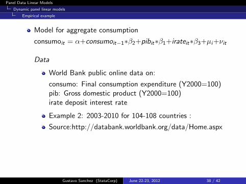
Model for aggregate consumption
consumoit = α+consumoit−1∗β2+pibit∗β1+irateit∗β3+µi+νit
Data
World Bank public online data on:
consumo: Final consumption expenditure (Y2000=100)pib: Gross domestic product (Y2000=100)irate deposit interest rate
Example 2: 2003-2010 for 104-108 countries :
Source:http://databank.worldbank.org/data/Home.aspx
Gustavo Sanchez (StataCorp) June 22-23, 2012 38 / 42

Panel Data Linear Models
Dynamic panel linear models
Empirical example
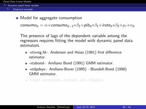
Model for aggregate consumption
consumoit = α+consumoit−1∗β2+pibit∗β1+irateit∗β3+µi+νit
The presence of lags of the dependent variable among theregressors requires fitting the model with dynamic panel dataestimators.
-xtivreg,fd-: Anderson and Hsiao (1981) first differenceestimator.
-xtabond-: Arellano Bond (1991) GMM estimator.
-xtdpdsys-: Arellano-Bover (1995) - Blundell-Bond (1998)GMM estimator.
-xtdpd- generalizes -xtabond- and -xtdpdsys-.
Gustavo Sanchez (StataCorp) June 22-23, 2012 39 / 42

Panel Data Linear Models
Dynamic panel linear models
Empirical example
Model for aggregate consumption
consumoit = α+consumoit−1∗β2+pibit∗β1+irateit∗β3+µi+νit
The presence of lags of the dependent variable among theregressors requires fitting the model with dynamic panel dataestimators.
-xtivreg,fd-: Anderson and Hsiao (1981) first differenceestimator.
-xtabond-: Arellano Bond (1991) GMM estimator.
-xtdpdsys-: Arellano-Bover (1995) - Blundell-Bond (1998)GMM estimator.
-xtdpd- generalizes -xtabond- and -xtdpdsys-.
Gustavo Sanchez (StataCorp) June 22-23, 2012 39 / 42

Panel Data Linear Models
Dynamic panel linear models
Empirical example - Arellano-Bond
Arellano-Bond
. xtabond lconsumo lpib lirate ,lags(1) maxldep(4) vsquish
Arellano-Bond dynamic panel-data estimation Number of obs = 550Group variable: country Number of groups = 104Time variable: year
Obs per group: min = 1avg = 5.288462max = 6
Number of instruments = 21 Wald chi2(3) = 5583.65Prob > chi2 = 0.0000
One-step results
lconsumo Coef. Std. Err. z P>|z| [95% Conf. Interval]
lconsumoL1. .2003175 .036051 5.56 0.000 .1296588 .2709762lpib .7843574 .0394084 19.90 0.000 .7071183 .8615965
lirate -.0109575 .0032787 -3.34 0.001 -.0173837 -.0045313_cons .2193715 .3215974 0.68 0.495 -.4109479 .8496908
Instruments for differenced equationGMM-type: L(2/5).lconsumoStandard: D.lpib D.lirate
Instruments for level equationStandard: _cons
Gustavo Sanchez (StataCorp) June 22-23, 2012 40 / 42

Panel Data Linear Models
Dynamic panel linear models
Empirical example - Arellano-Bover/Blundell-Bond
Arellano-Bover/Blundell-Bond
. xtdpdsys lconsumo lpib lirate ,lags(1) maxldep(4) vsquish
System dynamic panel-data estimation Number of obs = 658Group variable: country Number of groups = 108Time variable: year
Obs per group: min = 1avg = 6.092593max = 7
Number of instruments = 27 Wald chi2(3) = 16278.38Prob > chi2 = 0.0000
One-step results
lconsumo Coef. Std. Err. z P>|z| [95% Conf. Interval]
lconsumoL1. .3169481 .0290153 10.92 0.000 .2600791 .373817lpib .6010134 .0288126 20.86 0.000 .5445417 .6574852
lirate .0010375 .003142 0.33 0.741 -.0051206 .0071957_cons 1.834053 .17602 10.42 0.000 1.48906 2.179046
Instruments for differenced equationGMM-type: L(2/5).lconsumoStandard: D.lpib D.lirate
Instruments for level equationGMM-type: LD.lconsumoStandard: _cons
Gustavo Sanchez (StataCorp) June 22-23, 2012 41 / 42

Panel Data Linear Models
Summary
Summary
Brief introduction to panel data linear models
Fitting the model in Stata
Testing and accounting for serial correlation andheteroskedasticity
Panel Unit root tests - Model in first differences
Dynamic panel linear models
Gustavo Sanchez (StataCorp) June 22-23, 2012 42 / 42

Panel Data Linear Models
References
References
Anderson and Hsiao 1981. Estimation of dynamic models with errorcomponents. Journal of the American Statistical Association 76:598—606
Arellano, M. and S. Bond. 1991. Some tests of specification for panel data:Monte Carlo evidence and an application to employment equations. TheReview of Economic Studies 58: 277—297.
Arellano, M. and O. Bover. 1995. Another look at the instrumental variableestimation of error-components models. Journal of Econometrics 68: 29—51.
Blundell, R. and S. Bond. 1998. Initial conditions and moment restrictions indynamic panel data models. Journal of Econometrics 87: 115—43.
Drukker, D. M. 2003. Testing for serial correlation in linear panel-data models.Stata Journal 3: 168—177.
Poi and Wiggins 2001. http://www.stata.com/support/faqs/stat/panel.html
Wooldridge, J. M. 2002. Econometric Analysis of Cross Section and PanelData. Cambridge, MA: MIT Press
World Bank DataBank http://databank.worldbank.org/data/Home.aspx
Gustavo Sanchez (StataCorp) June 22-23, 2012 43 / 42


![[ME] Multilevel Mixed Effects - Stata · PDF file[XT] Stata Longitudinal-Data/Panel-Data Reference Manual [ME] Stata Multilevel Mixed-Effects Reference Manual [MI] Stata Multiple-Imputation](https://img.pdfslide.us/doc/110x75/5a78a96c7f8b9a7b698e4b38/me-multilevel-mixed-effects-stata-xt-stata-longitudinal-datapanel-data-reference.jpg)
![[ME] Multilevel Mixed Effects - Survey Design · 2016. 2. 16. · Stata, , Stata Press, Mata, , and NetCourse are registered trademarks of StataCorp LP. Stata and Stata Press are](https://img.pdfslide.us/doc/110x75/6119d35ebac5e41ff76887ce/me-multilevel-mixed-effects-survey-design-2016-2-16-stata-stata-press.jpg)