Fishing for the Right Words: Decision Rules for Human

Fishing for the Right Words: Decision Rules for HumanForaging Behavior in Internal Search Tasks

Andreas Wilke,a,b John M. C. Hutchinson,a,c Peter M. Todd,a,d

Uwe Czienskowskia

aCenter for Adaptive Behavior and Cognition, Max Planck Institute for Human DevelopmentbCenter for Behavior, Evolution and Culture, UCLA Department of Anthropology

cState Museum of Natural History GorlitzdSchool of Informatics and Cognitive Science Program, Indiana University

Received 25 February 2008; received in revised form 30 September 2008; accepted 21 October 2008

Abstract

Animals depleting one patch of resources must decide when to leave and switch to a fresh patch.

Foraging theory has predicted various decision mechanisms; which is best depends on environmental

variation in patch quality. Previously we tested whether these mechanisms underlie human decision

making when foraging for external resources; here we test whether humans behave similarly in a cog-

nitive task seeking internally generated solutions. Subjects searched for meaningful words made from

random letter sequences, and as their success rate declined, they could opt to switch to a fresh sequence.

As in the external foraging context, time since the previous success and the interval preceding it had a

major influence on when subjects switched. Subjects also used the commonness of sequence letters as

a proximal cue to patch quality that influenced when to switch. Contrary to optimality predictions,

switching decisions were independent of whether sequences differed little or widely in quality.

Keywords: Optimal foraging theory; Marginal Value Theorem; Patch leaving; Decision rule; Rule of

thumb; Ecological rationality; Information foraging; Information scent; Patchy environment;

Aggregation; Human bevioral ecology

1. Introduction

When should we move on to greener pastures? Humans and other animals face decisions

of this type in a variety of common domains. Whenever resources are distributed in space or

time, and a local source can be depleted faster than it replenishes, it is important to decide

when one could do better by switching to a different source. This is particularly clear in the

Correspondence should be sent to Andreas Wilke, Center for Adaptive Behavior and Cognition, Max Planck

Institute for Human Development, Lentzeallee 94, 14195 Berlin, Germany. E-mail: [email protected]

Cognitive Science 33 (2009) 497–529Copyright � 2009 Cognitive Science Society, Inc. All rights reserved.ISSN: 0364-0213 print / 1551-6709 onlineDOI: 10.1111/j.1551-6709.2009.01020.x

case of clumpy distributions of food items: foraging woodpeckers must decide when to give

up looking for grubs in one tree and fly off to another, and people searching for blackberries

must assess whether there are any more ripe berries easy to reach on the current plant or if it

is better to move to the next.

In addition to these traditional types of foraging in patchy environments studied by bio-

logists and anthropologists (e.g., Bell, 1991; Winterhalder & Smith, 1981), humans spend

much of their time seeking information resources that are also often structured in patches.

These information patches may be found internally, in one’s memory, or externally, such as

in an office or library, in the minds of friends and family, or on the Web. The information

that a forager is looking for comes in variable quantities that are concealed in remembered

semantic categories, piles of papers, file drawers, bookshelves, libraries, computer files, the

heads of different colleagues, or online data collections, all of which can differ in how long

it takes to get from one ‘‘location’’ to another and in the rate at which each provides infor-

mation (e.g., Pirolli & Card, 1999; Sandstrom, 1994, 1999).

How can the information seeker decide when a particular patch is unlikely to yield

anything else useful very quickly and that it is better to move on to another? Like animals

maximizing their rate of energy intake, optimal information foragers might maximize the

long-term rate of valuable information gained per unit time, given the constraints of the task

environment they face (e.g., the information returns of different sources and the costs of

finding and accessing them). Pirolli and Card (1997) suggested, using an evolutionary

ecological perspective to study information-gathering strategies, ‘‘treating adaptations to

the flux of information in the cultural environment in much the same manner as biologists

study adaptations to the flux of energy in the physical environment’’ (p. 643). This also fits

within the broader study of ecological rationality, the adaptive fit of decision mechanisms to

the information structure of particular environments (Gigerenzer, Todd, & the ABC

Research Group, 1999; Todd & Gigerenzer, 2007).

Here we adopt this approach to study the question of what mechanisms people have for

moving through a succession of cognitive information-foraging tasks: seeking anagrams in a

‘‘patch’’ of letters. As with the feeding-patch and web-search paradigms, reward rate declines

with time spent in each patch, so that at some point it is better to switch to the next patch

despite the ‘‘travel’’ costs. Do people use similar rules when rewards are produced by think-

ing and searching in internal memory rather than by exploring the external environment? To

find out, we first review prior work from the biology, anthropology, and psychology litera-

tures on foraging behavior and patch time allocation in humans and other animals, and then

describe our previous study on the rules people use to decide when to switch from one (exter-

nal) fishing pond to another (Hutchinson, Wilke, & Todd, 2008). Next we introduce our inter-

nal-foraging anagram task used here. We show that people use the same main cues to make

patch-leaving decisions in both of these very different types of domain.

1.1. From models of optimal foraging to decision rules in discrete resource environments

The adaptive problem of finding resources is crucial for all animals. Natural resources are

often distributed in fairly distinct patches (i.e., local areas with high probability of resource

498 A. Wilke et al. ⁄ Cognitive Science 33 (2009)

encounter that are surrounded by other areas where the probability of resource encounter is

at or near zero). Animals feeding on such resources need to make decisions not only on

where to forage but also on how long they should forage in a particular patch. At what point

is it better to leave a patch and travel to a new one? If a bird has found nearly all the berries

on a bush, staying longer on that bush is wasteful because too much time is lost in finding

the next berry: it is better to move to another bush where the initial gain rate is higher.

Conversely it is wasteful to leave too early, because then too much time is taken up with

traveling to new bushes. What the bird needs is a decision rule determining the appropriate

moment of departure from the patch.

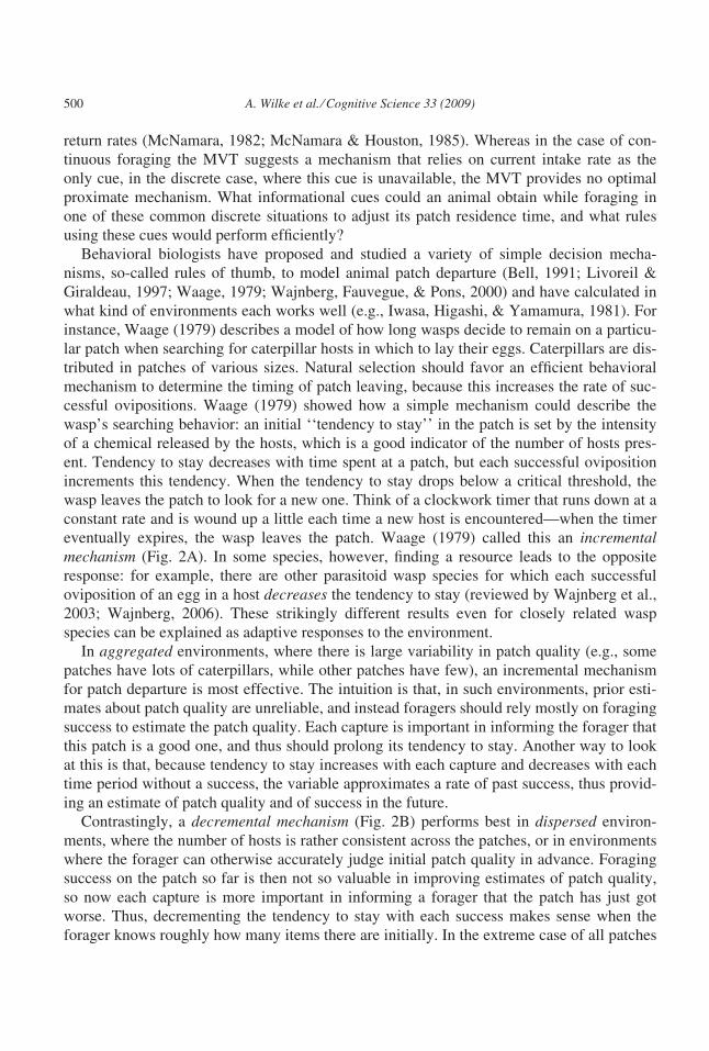
Classical optimal foraging theory addresses the patch-leaving decision that would maxi-

mize the bird’s fitness. Specifically, Charnov’s Marginal Value Theorem (MVT; Charnov,

1976) states that the optimal strategy for each individual is to leave a patch when the instan-

taneous rate of return (e.g., of food) from the current patch falls below the mean return rate

from the environment when following the optimal strategy. When an animal first enters a

rich patch, gains from exploiting it are high, because the resources are initially plentiful and

easy to find. As time passes, however, the forager depletes non-renewing resources and it

takes longer and longer to find the next item. This declining rate of resource gain can be

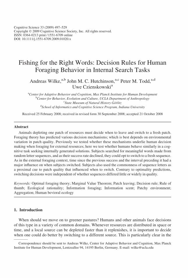
represented by a graph in which the gain curve levels off (Fig. 1). When the travel time

between patches is taken into account, the optimal time to leave can be computed.

Whereas the qualitative predictions of the MVT have often been verified (e.g., Stephens

& Krebs, 1986), its assumptions about the information available to foragers may be unrealis-

tic: animals do not necessarily have complete knowledge of the abundance and distribution

of resources in the habitat (e.g., when exploring a new environment), so they do not know

the maximum mean rate of return in that environment. Furthermore, for many animals, for-

aging involves finding discrete items that are encountered stochastically, so that the instanta-

neous return rate translates to a probability that is only indirectly estimated from recent

Fig. 1. The Marginal Value Theorem. The concave-down shape of the gain curve arises, for instance, from

resource depletion; where the tangent AB touches the gain curve defines the optimal patch residence time Topt

(adapted from Charnov, 1976).

A. Wilke et al. ⁄ Cognitive Science 33 (2009) 499

return rates (McNamara, 1982; McNamara & Houston, 1985). Whereas in the case of con-

tinuous foraging the MVT suggests a mechanism that relies on current intake rate as the

only cue, in the discrete case, where this cue is unavailable, the MVT provides no optimal

proximate mechanism. What informational cues could an animal obtain while foraging in

one of these common discrete situations to adjust its patch residence time, and what rules

using these cues would perform efficiently?

Behavioral biologists have proposed and studied a variety of simple decision mecha-

nisms, so-called rules of thumb, to model animal patch departure (Bell, 1991; Livoreil &

Giraldeau, 1997; Waage, 1979; Wajnberg, Fauvegue, & Pons, 2000) and have calculated in

what kind of environments each works well (e.g., Iwasa, Higashi, & Yamamura, 1981). For

instance, Waage (1979) describes a model of how long wasps decide to remain on a particu-

lar patch when searching for caterpillar hosts in which to lay their eggs. Caterpillars are dis-

tributed in patches of various sizes. Natural selection should favor an efficient behavioral

mechanism to determine the timing of patch leaving, because this increases the rate of suc-

cessful ovipositions. Waage (1979) showed how a simple mechanism could describe the

wasp’s searching behavior: an initial ‘‘tendency to stay’’ in the patch is set by the intensity

of a chemical released by the hosts, which is a good indicator of the number of hosts pres-

ent. Tendency to stay decreases with time spent at a patch, but each successful oviposition

increments this tendency. When the tendency to stay drops below a critical threshold, the

wasp leaves the patch to look for a new one. Think of a clockwork timer that runs down at a

constant rate and is wound up a little each time a new host is encountered—when the timer

eventually expires, the wasp leaves the patch. Waage (1979) called this an incrementalmechanism (Fig. 2A). In some species, however, finding a resource leads to the opposite

response: for example, there are other parasitoid wasp species for which each successful

oviposition of an egg in a host decreases the tendency to stay (reviewed by Wajnberg et al.,

2003; Wajnberg, 2006). These strikingly different results even for closely related wasp

species can be explained as adaptive responses to the environment.

In aggregated environments, where there is large variability in patch quality (e.g., some

patches have lots of caterpillars, while other patches have few), an incremental mechanism

for patch departure is most effective. The intuition is that, in such environments, prior esti-

mates about patch quality are unreliable, and instead foragers should rely mostly on foraging

success to estimate the patch quality. Each capture is important in informing the forager that

this patch is a good one, and thus should prolong its tendency to stay. Another way to look

at this is that, because tendency to stay increases with each capture and decreases with each

time period without a success, the variable approximates a rate of past success, thus provid-

ing an estimate of patch quality and of success in the future.

Contrastingly, a decremental mechanism (Fig. 2B) performs best in dispersed environ-

ments, where the number of hosts is rather consistent across the patches, or in environments

where the forager can otherwise accurately judge initial patch quality in advance. Foraging

success on the patch so far is then not so valuable in improving estimates of patch quality,

so now each capture is more important in informing a forager that the patch has just got

worse. Thus, decrementing the tendency to stay with each success makes sense when the

forager knows roughly how many items there are initially. In the extreme case of all patches


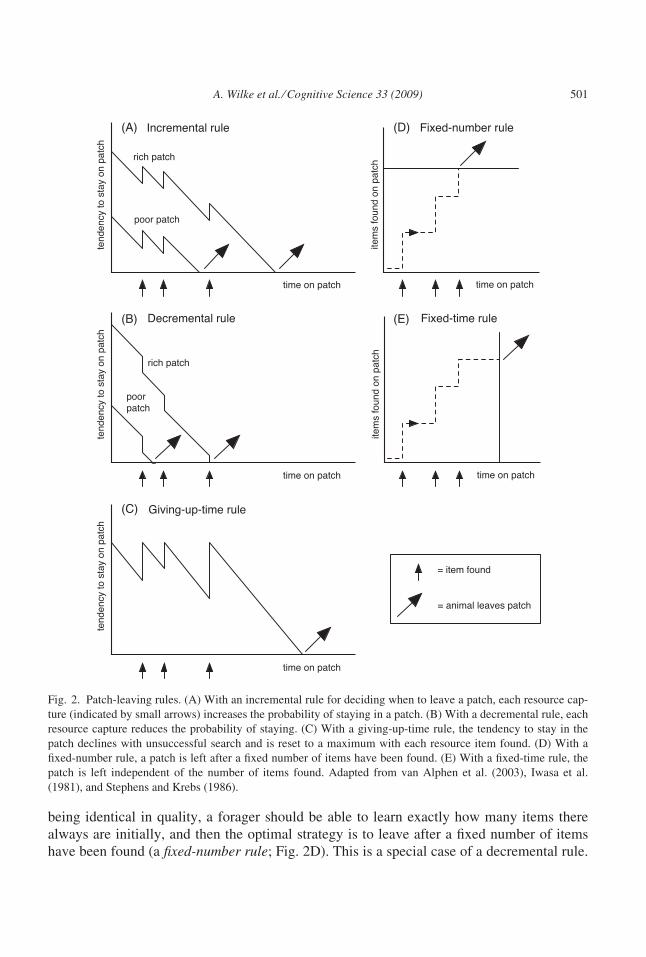
being identical in quality, a forager should be able to learn exactly how many items there

always are initially, and then the optimal strategy is to leave after a fixed number of items

have been found (a fixed-number rule; Fig. 2D). This is a special case of a decremental rule.

Fig. 2. Patch-leaving rules. (A) With an incremental rule for deciding when to leave a patch, each resource cap-

ture (indicated by small arrows) increases the probability of staying in a patch. (B) With a decremental rule, each

resource capture reduces the probability of staying. (C) With a giving-up-time rule, the tendency to stay in the

patch declines with unsuccessful search and is reset to a maximum with each resource item found. (D) With a

fixed-number rule, a patch is left after a fixed number of items have been found. (E) With a fixed-time rule, the

patch is left independent of the number of items found. Adapted from van Alphen et al. (2003), Iwasa et al.

(1981), and Stephens and Krebs (1986).


When the number of items present initially is known perfectly, the number of captures

allows accurate calculation of the number left, which determines the expected success rate

were the forager to remain, and thus whether it is better to leave.

Another special case is the point along the continuum between aggregated and dispersed

environments where items are randomly distributed over patches according to a Poisson dis-

tribution. At this balance point between environments where the optimal rule is incremental

or decremental, the optimum is instead a fixed-time rule, to leave after a fixed time regard-

less of foraging success (Fig. 2E).

In other empirical work, Krebs, Ryan, and Charnov (1974) modeled patch departure in

birds using a giving-up-time rule (i.e., the tendency to stay in a patch declines with unsuc-

cessful search, and it is reset to the maximum with each resource item found; see Fig. 2C).

Compatible with this rule (although also with others), a bird’s mean giving-up time (interval

on the patch without a capture prior to departure) did not differ significantly between patch

types differing in their initial quantity of resources. This rule, like the incremental rule,

works best when patches vary widely in quality and patches are hard to assess in advance.

This is because both rules use past success rate to judge future success rate, rather than rely-

ing on prior judgments of patch quality. With the incremental rule, past success rate is

judged from number of captures and time spent, whereas with a giving-up-time rule, the

interval without a capture provides the estimate of current rate of capture. Interval without a

capture or between earlier captures could be used as cues in more complex rules, but the

classic giving-up-time rule specifies switching whenever the interval without a capture

exceeds a fixed threshold.

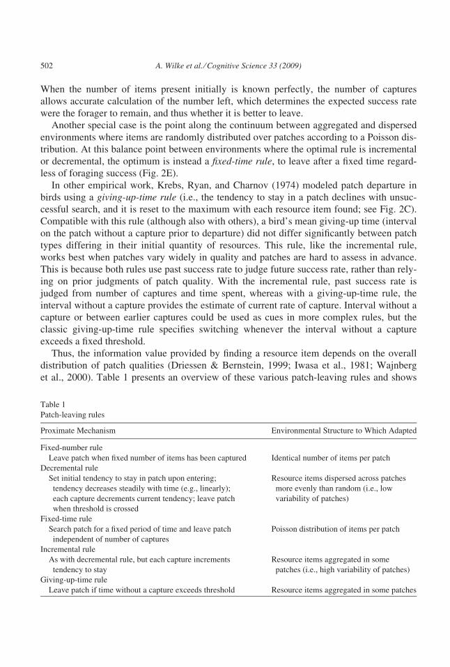
Thus, the information value provided by finding a resource item depends on the overall

distribution of patch qualities (Driessen & Bernstein, 1999; Iwasa et al., 1981; Wajnberg

et al., 2000). Table 1 presents an overview of these various patch-leaving rules and shows

Table 1

Patch-leaving rules

Proximate Mechanism Environmental Structure to Which Adapted

Fixed-number rule

Leave patch when fixed number of items has been captured Identical number of items per patch

Decremental rule

Set initial tendency to stay in patch upon entering;

tendency decreases steadily with time (e.g., linearly);

each capture decrements current tendency; leave patch

when threshold is crossed

Resource items dispersed across patches

more evenly than random (i.e., low

variability of patches)

Fixed-time rule

Search patch for a fixed period of time and leave patch

independent of number of captures

Poisson distribution of items per patch

Incremental rule

As with decremental rule, but each capture increments

tendency to stay

Resource items aggregated in some

patches (i.e., high variability of patches)

Giving-up-time rule

Leave patch if time without a capture exceeds threshold Resource items aggregated in some patches


how the environmental continuum maps onto a continuum of optimal strategies plus the

giving-up-time rule.

1.2. Prior work on human patch-leaving behavior in biology, anthropology, and psychology

Behavioral ecologists have applied the theory detailed above to a wide range of animals,

particularly birds and parasitoid insects (e.g., Nonacs, 2001; Wajnberg, 2006). However,

besides our own work (Hutchinson et al., 2008) described below, we know of only one

paper from this discipline examining patch leaving in humans (Hart & Jackson, 1986).

That neatly involved subjects foraging for sultanas suspended on a series of artificial trees.

Biological anthropology provides a rich body of findings on foraging decisions among

hunter-gatherers (e.g., Kelly, 1995; Winterhalder & Smith, 1981). Most of the work, how-

ever, deals with environmental variables and how they systematically relate to foragers’ diet

or how foragers arrive at subsistence decisions based on the available choice of resources.

Some studies on traditional foragers’ decision making also incorporated the logic of the

MVT (e.g., Burger, Hamilton, & Walker, 2005; Metcalfe & Barlow, 1992), but without

addressing patch leaving in terms of particular decision mechanisms.

In psychology, although there is work on visual search behavior (e.g., Gilchrist, North, &

Hood, 2001; Klein, 2000), group foraging (Goldstone & Ashpole, 2004; Goldstone,

Ashpole, & Roberts, 2005), and consumers as foragers (Rajala & Hantula, 2000; Smith &

Hantula, 2003), almost no research deals with the rules people utilize when deciding how

long to remain in one patch before moving to a different one. One exception is research on

task switching (e.g., changing from one television channel to another; see Wang, Busemey-

er, & Lang, 2006). However, this usually conceptualizes the problem as an interleaving

between two different and unrelated tasks (e.g., Rogers & Monsell, 1995). This possibility

of switching back and forth considerably changes the problem, becoming more akin to the

matching paradigm, especially when switching does not include a cost (e.g., travel time).

This is the case in the study by Payne, Duggan, and Neth (2007), who examined switching

between two anagram tasks very similar to those we use. Our experience of solving such

puzzles ourselves is that taking a break often facilitates finding solutions when coming back

to the problem (maybe the subconscious is working away in the meantime, or maybe a fresh

perspective helps; either would explain why the subjects switched almost as often in a con-

dition when total time at each patch was fixed); so there could even be an extra benefit to

switching when returning is allowed. Nevertheless, with or without returns, it is still usually

the case that past foraging success at the current patch should be used to estimate future

success rate if you remain.

Also directly relevant is research from operant experiments in which people make

repeated choices between a progressive-ratio schedule and a fixed-ratio schedule (e.g.,

Wanchisen, Tatham, & Hineline, 1992). Because choosing from the fixed-ratio schedule

resets the progressive-ratio schedule, the situation is analogous to patch leaving.

Research in this area also compared behavior against optimality predictions, but the

focus has been mainly on assessing species differences in the sensitivity to delayed

outcomes.


Some significant work on patch-leaving mechanisms is found in the area of information

foraging (Pirolli, 2005, 2007). In addition to the general problem of deciding when to give

up on a specific Web locality and move on to the next, Pirolli (2007) also discusses how

Internet users may assess the quality of an information source from proximal cues (e.g.,

words contained in links to search results). These cues are put together into an overall

assessment of search-path quality that Pirolli calls information scent. Although Pirolli does

not specify the exact rule people use to decide when to move to the next information patch,

he hypothesizes that information scent influences whether to leave or stay, similar to the

way that scent of caterpillar hosts determined the initial tendency to stay in our earlier

example (Waage, 1979).

1.3. Decision rules for external and internal search tasks

Given the lack of research on the mechanisms humans use to decide how best to exploit

patchy resources, along with the wealth of results on the mechanisms that other animals

should and do use, we pose the following questions in our research:

1. What kind of decision rules do humans use in patchy environments?

2. Are humans sensitive to environmental variation and can they adapt their patch-

leaving rules to the types of environments they face? Whereas most animals tend to

be specialists and thus could use hardwired rules adapted to how food naturally

occurs in their particular environment, humans are generalists. This means that

humans may have evolved to feed on some foods that are evenly dispersed across

patches and on some that are aggregated in a few high-quality patches amidst many

poor patches. Consequently, for food-related searches at least, humans may be able

to tell what kind of environment structure they are facing, and respond accordingly.

3. Do humans search for items in internal ‘‘cognitive’’ space using the same patch-

leaving rules that they use for items in external ‘‘physical’’ space? There is some rea-

son to believe that the mechanisms that evolved for the latter may have been co-opted

for use in cognitive domains as well (Hills, 2006; Hills, Todd, & Goldstone, 2008b).

4. What cues (e.g., the number of found resource items or the time interval between pre-

vious captures) do people use to assess the quality of a patch? Do people use some

cues to set an initial tendency to stay in a patch even prior to searching for individual

resource items?

To answer these questions we have designed two human experiments that differ in

whether search is external (e.g., for physical objects) or internal (e.g., for words ⁄ items in

memory), but for which the environmental parameters (e.g., travel times, mean reward rates)

are closely matched (Wilke, 2006; Wilke, Hutchinson, & Todd, 2004). In both experiments,

we varied the distribution of items across patches, to test whether humans can adapt their

rules appropriately.

In the first experiment, the Fishing Task (Hutchinson et al., 2008), subjects were

presented with a virtual landscape on a computer screen allowing them to ‘‘forage’’ at a


succession of ponds (i.e., patches). While remaining at a pond, a subject would attempt to

catch fish that appeared at stochastic intervals dependent on the number of fish left in that

pond; whenever the subject chose to leave a pond (e.g., because the fewer remaining fish

were taking longer to appear), it took a fixed amount of travel time to ‘‘walk’’ to the next

pond. All ponds looked the same, but the initial number of fish per pond varied according to

three different resource distributions (i.e., evenly dispersed, aggregated, Poisson). The

results showed that subjects used patch-leaving rules that are adaptive in an aggregated

environment, no matter which distribution they faced. Switching after a fixed number of

items (as predicted for the evenly dispersed environment) or switching after a fixed time (as

predicted for the Poisson environment) was not observed.

In the second experiment, the Word Puzzle Task presented here, foraging for fish was

replaced by finding solutions to a modified anagram puzzle. The set-up of this search over

patches of internally generated solutions was kept close to that of the Fishing Task, so that

we could address the differences between external and internal search, along with uncover-

ing the particular patch-leaving mechanisms used in this search domain.

2. Method

In our computer-based Word Puzzle Task, German-speaking subjects were presented

with a succession of letter sequences and asked to generate meaningful German words out

of each sequence in turn. They could use all or only some of the letters in a sequence as long

as they used each letter only once for each solution.

Subjects could generate words from each letter sequence for as long as they wanted and

were paid for each meaningful word found. Some valid solutions were more difficult to spot

than others, and there was only a finite number of solutions for each letter sequence, so sub-

jects needed to decide at what point they wanted to switch to a new sequence owing to the

diminishing returns from the current sequence (i.e., patch). Switching sequences was made

costly by including a constant time delay (i.e., the travel time) between sequences.

It was impossible to create resource distributions for this task that exactly mirrored

those in our Fishing Task, because we did not have control of when Word Puzzle solu-

tions ‘‘appeared’’ to our subjects. The best we could do was to manipulate the degree of

aggregation in sequence quality. First, we generated sequences at random and then gave

those sequences to an initial round of subjects (the ‘‘sequence-selection study’’). The

results confirmed that the number of available solutions correlated well with the rate at

which subjects found solutions, so we used the former as a measure of ‘‘quality’’ by

which sequences were ranked. By selecting from the ranking we constructed two

resource distributions. The ‘‘dispersed’’ environment was limited to sequences of med-

ium quality, whereas the ‘‘aggregated’’ environment used a mixture of high- and low-

quality sequences (see details below). Finally, a second round of subjects experienced

either the dispersed or the aggregated environment in the main experiment. Conditions in

the sequence-selection study and the main experiment were very similar (except where

mentioned below).


The resource environments that are usually considered in the animal literature assume

that the successful capture of one item is independent from finding another item. In the

Word Puzzle this assumption was liable to be violated, because finding one solution could

lead subjects to find more words that are closely associated forms of this original word (e.g.,

the plural or a different case of the word). To reduce this tendency, only singular nouns in

the nominative case were allowed as valid solutions. Furthermore, the minimum length of

an acceptable word was set to four letters so that subjects would not come up with the same

(easy) solutions for different sequences and switch before trying to find more sophisticated

words.

2.1. Sequence and wordlist generation

The length of the letter sequences was fixed at nine letters, always six consonants and

three vowels; our aim was that sequences would thus initially appear similar in difficulty,

and hence quality (even though they actually differed). Within each sequence, a letter could

appear only once. Letters with the lowest letter frequencies in the German language were

excluded, as this information could readily be utilized as a cue to the difficulty of a

sequence (i.e., the letters J, Q, X, and Y with letter frequencies of 0.27, 0.02, 0.04, and

0.08 percent, respectively; see Bauer, 2000). We generated a list of 70 distinct letter

sequences following the above criteria. No letters with German umlauts occurred within

these sequences.

A wordlist was compiled that contained all the possible meaningful word solutions from

the set of sequences. For this purpose, two professional linguistic lists were merged to pro-

duce one master list containing more than 235,000 words (Czienskowski, 2005a; for a

detailed description see Wilke, 2006). This merged list was subsequently shortened (e.g., by

taking out duplicates, words with duplicate letters, and words that were not four to nine let-

ters in length) and then compared against all the possible letter combinations created by

each of the 70 sequences. Letter combinations from a sequence that were also found in the

shortened word list were kept and put into a provisional solution list. This list was then

given to German native speakers for checking and correction (e.g., to ensure that entries

were singular nouns). The final list of meaningful word solutions had 1,149 entries.

2.2. Participants

Subjects participated in the sequence-selection study and the main experiment at the Max

Planck Institute for Human Development in Berlin, Germany. Subjects were German native

speakers who self-reported not suffering from dyslexia. To collect the data on sequence

quality, 26 subjects (13 women, 13 men) were presented with sequences in a structured-

random order (to ensure that all sequences were seen similarly often). For the main study,

60 subjects (31 women, 29 men) were each randomly assigned to either the dispersed or

aggregated environment. Average age was 25.3 years (SD = 3.6). Subjects were paid at the

end of the experiment dependent on the total number of solutions that they found (receiving

€0.20 per solution plus a show-up fee of €4.00).


2.3. Materials

All experimental materials, including instructions and training session, were presented on

a computer screen (Czienskowski, 2005b). Instructions were the same in both experimental

conditions and informed subjects about the composition of the letter sequences (e.g., length,

vowel-to-consonant ratio), what kind of words were valid solutions (i.e., German singular

nouns in the nominative case), and how they could move from one sequence to the next.

Subjects were also informed about special invalid cases such as the names of persons, geo-

graphical places, and verb infinitives. As a comprehension check, subjects worked through a

25-item quiz on these rules. Each quiz item was an example of a word they might type in

and subjects had to judge if it would be allowed. There was no penalty for making mistakes

on the quiz, but subjects had to correct their mistakes before being allowed to continue to

the training session.

Subjects were told that sequences varied in the number of valid solutions available. The

instructions stated that they could see an unlimited number of letter sequences, but that there

was no going back to an earlier sequence. As in the Fishing Task (Hutchinson et al., 2008),

subjects were informed that the timing of when they switched from one letter sequence to

the next would crucially influence their final payoff and that they should avoid two

extremes: switching too early or staying too long at each sequence.

2.4. Procedure

Subjects had to put aside their watches and cell phones so that they would have no access

to an external time-keeper. They worked through the onscreen instructions, the training

quiz, and an explanation of the screen set-up at their own pace. A 4 min training session fol-

lowed, which was identical to the main experiment. The order of sequences was constant in

the training session but randomly varied in the experimental part. Each letter sequence

appeared at the center of the screen and subjects then typed solutions into an entry field

located directly underneath the sequence (Fig. 3).

If subjects entered a solution that was in the word list, they received visual feedback in

the form of a green circle along with the announcement ‘‘Correct!’’ and the entry field was

automatically cleared to make way for a new entry. If they entered an invalid word, a red

circle and the word ‘‘Incorrect!’’ appeared instead, along with specific feedback about the

kind of error made (i.e., word entry too short, multiple use of the same letter, use of a letter

not in the sequence, invalid spelling out of umlauts, or word already entered for this

sequence). In all other cases, the entered word was reported to be not in our word list. Incor-

rect entries remained in the entry field to be edited or deleted. Subjects were informed that,

in case of erroneous rejections of valid solutions, they should continue with the experiment

anyhow. Each accepted solution was transferred to the word stack after entry (Fig. 3, right

side). This stack was emptied when subjects switched to a new sequence.

At any time, subjects could decide to switch to a new sequence by clicking on the red

‘‘New sequence?’’ button (Fig. 3, lower right). Upon clicking on the button, a bouncing ball

animation saying ‘‘Please wait!’’ appeared on an empty screen and subjects had to wait for


25 s. Then, the experimental screen reappeared showing a new letter sequence. The experi-

mental session continued for 60 min or until all 26 sequences available for that condition

had appeared.

Following the experimental session, subjects in the main experiment filled out a question-

naire and performed an additional estimation task. The onscreen questionnaire asked sub-

jects whether they came up with a particular strategy to determine their patch leaving and, if

yes, how they would describe it. Further questions asked subjects to rate (on a four-point

scale from none to very often) their use of three cues in determining when to switch to the

next letter sequence: the number of correct words found in the current sequence, the time

spent in the current sequence, and the time interval since the previous word was found.

The final estimation task provided us with information on how subjects initially assessed

the quality of a letter sequence before trying to find solutions. We presented subjects with

half of the sequences from the environment they had not seen. Subjects were asked for each

sequence to estimate rapidly how many solutions they would be able to find. The sequences

were presented in a random order and appeared sequentially. There was no time restriction

for answering, but each sequence was masked after a presentation of 10 s.

2.5. Quality of the wordlist and sequence selection

In the initial sequence-selection study, 35% (across participants, SD = 14%) of word

entries were incorrect. These invalid entries were analyzed and coded into five categories:

17% contained letters that were not part of the sequence or used a letter twice, 48% were

errors that violated our word criteria (e.g., plurals or nonnominative cases), 1% were repeti-

tion errors, 31% were nonsense words, and 3% were words that should have been allowed

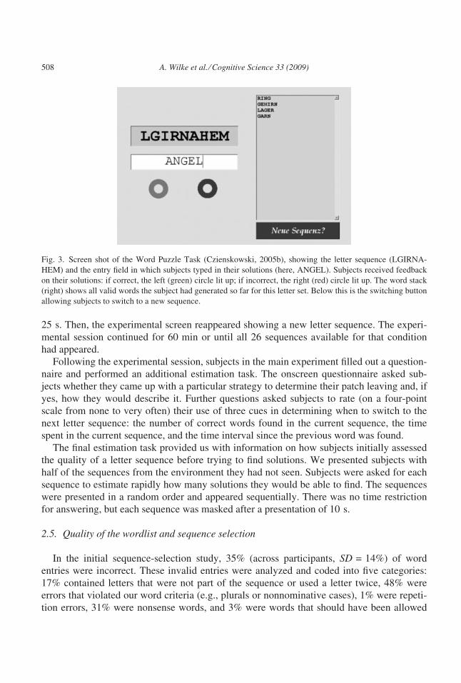
Fig. 3. Screen shot of the Word Puzzle Task (Czienskowski, 2005b), showing the letter sequence (LGIRNA-

HEM) and the entry field in which subjects typed in their solutions (here, ANGEL). Subjects received feedback

on their solutions: if correct, the left (green) circle lit up; if incorrect, the right (red) circle lit up. The word stack

(right) shows all valid words the subject had generated so far for this letter set. Below this is the switching button

allowing subjects to switch to a new sequence.


but were flagged as errors because the wordlist did not contain them. We believe that the last

category was small enough to avoid subjects getting frustrated by erroneous word rejections;

furthermore, wrongly rejected words from the initial experiment were included in the solu-

tion list for the main experiment.

We reserved 10 sequences for use in the training session. For each of the remaining

60 sequences, we computed the mean number of solutions subjects found (with each

sequence seen by at least five subjects) and correlated this with the actual number of solu-

tions for each sequence in our wordlist. This correlation was strong (r = .81, p < .0001). To

further ensure that subjects would experience a consistent association between number of

solutions still to be found and rate at which they were finding those solutions, for each

sequence we calculated an average slope for this relationship and then dropped eight

sequences with values that were atypical for sequences of that quality. To make up numbers,

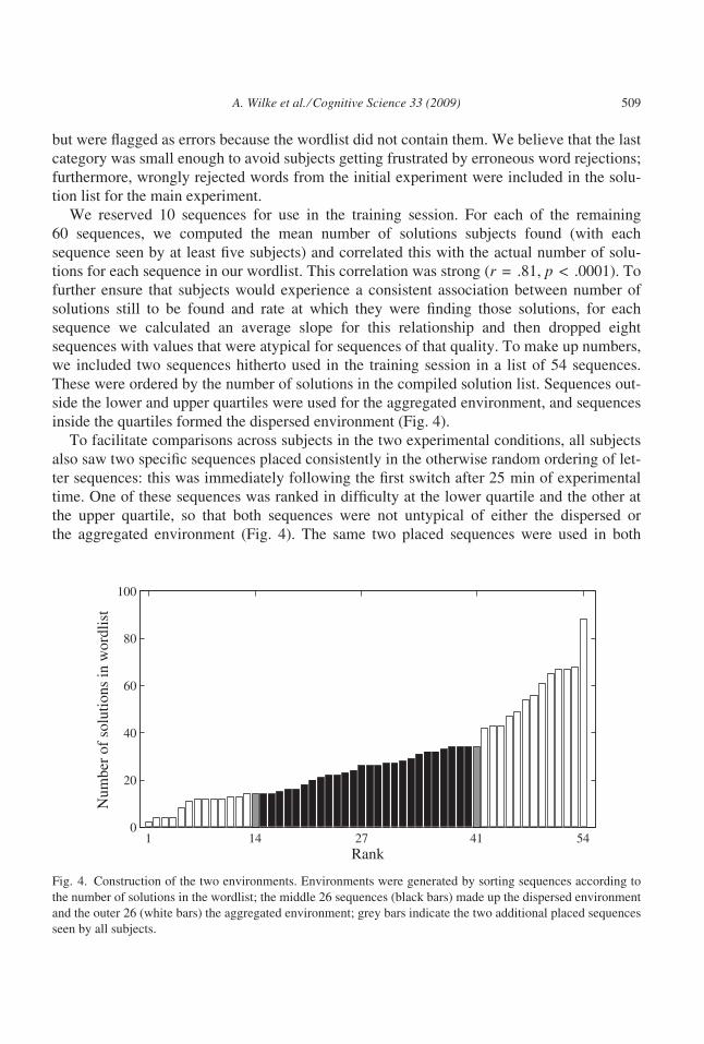
we included two sequences hitherto used in the training session in a list of 54 sequences.

These were ordered by the number of solutions in the compiled solution list. Sequences out-

side the lower and upper quartiles were used for the aggregated environment, and sequences

inside the quartiles formed the dispersed environment (Fig. 4).

To facilitate comparisons across subjects in the two experimental conditions, all subjects

also saw two specific sequences placed consistently in the otherwise random ordering of let-

ter sequences: this was immediately following the first switch after 25 min of experimental

time. One of these sequences was ranked in difficulty at the lower quartile and the other at

the upper quartile, so that both sequences were not untypical of either the dispersed or

the aggregated environment (Fig. 4). The same two placed sequences were used in both

Fig. 4. Construction of the two environments. Environments were generated by sorting sequences according to

the number of solutions in the wordlist; the middle 26 sequences (black bars) made up the dispersed environment

and the outer 26 (white bars) the aggregated environment; grey bars indicate the two additional placed sequences

seen by all subjects.


experimental conditions and appeared in a fixed order: the high-difficulty immediately fol-

lowed by the low-difficulty sequence.

3. Results

We expected that subjects would continue to gain in experience beyond the initial train-

ing session, and subsequent analyses reported below confirmed that the speed of finding

solutions and patterns of switching behavior changed over the course of the experimental

session. To focus our analyses on the strategies applied after subjects had learned about each

environment, we excluded sequences seen in the first 20 min of the experimental session

(cf. Hutchinson et al., 2008). This left a median of 13 sequences per subject for all further

analyses reported here (range: 4–20 sequences).

3.1. Initial analyses

Subjects stayed in each sequence for between 12 and 620 s (median: 138 s), and there

was no significant difference between environments in the geometric mean time (GLM of

log-transformed data; subject and sequence (both random factors) each nested within envi-

ronment (fixed); F[1,83] = 0.79, p = .38). However, residence time does show some sys-

tematic variation: subjects in the aggregated environment spent on average 1.7 times as long

on a sequence from the easy subset as on one from the difficult subset (GLM of log-trans-

formed data; subject and sequence random factors, sequence nested within subset (fixed);

F[1,27] = 52, p < .0001).

In our analogous Fishing Task experiment (Hutchinson et al., 2008), subjects usually left

patches too late, in the sense that they could have done better if they had left each patch

sooner; this mirrors an almost universal finding in studies of animal patch leaving (e.g.,

Nonacs, 2001). In that experiment, we could determine optimal patch-leaving times; here,

because gain curves and patch qualities are liable to vary across individuals, we compared

each individual’s performance against their possible performance if they had left each patch

earlier. We calculated the performance (number of solutions divided by the time spent,

including ‘‘travel time’’) a subject would have achieved when giving up after a proportion qof the time actually spent on each patch. Totaling across all sequences and subjects, perfor-

mance is highest when q is about .7, leading to a 10% advantage. If switching times had

been consistently .7 of those observed, 50 out of 60 subjects would have improved their

performance.

Each sequence that a subject saw resulted in a median of four solutions (maximum 20).

The median proportion of sequences that individual subjects left without finding a solution

was 9% in the dispersed environment and 15% in the aggregated environment. Individual

subjects discovered a median of 14% of the solutions in our wordlist for each sequence.

There were an appreciable number of erroneous entries, even after excluding sequences seen

in the first 20 min. The subject median was one error every 75 s of active searching, or

about one for every two solutions (see above for the kind of errors that subjects made).


The median giving-up time between entering the last correct solution for a sequence and

switching was 38 s. In our Fishing Task experiment (Hutchinson et al., 2008), we found a

strong bimodality in this interval, because subjects often switched right after catching a fish,

particularly when they had been waiting for a long time without success, as though they had

decided to switch then while waiting. However, such switching immediately after a success

was rare in the Word Puzzle experiment.

3.2. Estimation task

Theory predicts that any valid external cues to the quality of a patch should affect the

switching decision (e.g., van Alphen, Bernstein, & Driessen, 2003; Pirolli, 2007; Shaltiel &

Ayal, 1998; Waage, 1979). Such cues should be used by subjects when we asked them (at

the end of the experiment) to estimate quickly the number of solutions to sequences that

they had not already seen. These estimates averaged over subjects correlate well with,

although considerably underestimate, the number of available solutions for each sequence

(�rS = .48, averaging the correlations calculated separately for each environment). We found

that the mean letter frequency of the sequence’s constituent letters in the German language

correlates highly with the estimates (�rS = .65) and with the actual number of solutions

(rS = .70). Thus, letter frequency may be a cue that people use to judge fairly accurately the

relative number of solutions they are likely to find in a sequence.

3.3. Checking the form of the gain curve

The Word Puzzle was designed to instantiate the decelerating gain rate found in typical

foraging situations, such that it should on average take longer to find each successive solu-

tion in a letter-sequence patch. To test this assumption, we related IN, the interval preceding

the Nth solution, to N by fitting the following curvilinear function:

IN ¼ siqjNQj expðatÞ

(derived from linear regression of ln[I] against ln[N] and t; R2 = .78). We allowed the rela-

tionship to be affected by si, describing intersubject variation in their speed of finding solu-

tions, and by qj and Qj, describing variation between sequences in the form of the gain

curve (i and j index subjects and sequences, respectively). Values of si and qj are constrained

by the fitting procedure to be positive and all fitted values of Qj were above 0 (median 1.2);

this confirms that in all sequences finding each successive solution indeed tends to take pro-

gressively longer. The coefficient a quantifies how success rate changes with time t of start-

ing a sequence after the beginning of the experiment. Unsurprisingly, experience speeds up

the rate of finding solutions, F(1,3125) = 34.9, p < .0001, but the fitted value of a implies

that solutions are found at a rate only 1.19 times faster after 50 min than after 20 min.

However, for this particular task, it is possible that even though the return rate decelerates

on average, finding one solution may make it easier to find another similar word that is also

a solution. If that were the case, then, in contrast to the idealized assumptions typically used


in foraging theory, rewards would be clustered in time. We had tried to minimize this

within-patch clumpiness by allowing only nouns in the nominative singular. To examine

how much it nevertheless remained, we compared the time to find the first solution in a

patch, when the solution-clustering effect must be absent, with the interval between finding

the first and second solutions, when the effect could sometimes occur, resulting in very brief

intervals. There is indeed an excess of brief (2–4 s) intervals preceding the second solution

compared with the first, but their rate of occurrence is limited to about 10–15%, so this envi-

ronment does not appear to differ substantially from the usual assumptions of foraging

theory.

3.4. Exploratory graphs

An initial step in analyzing the decision mechanism was to visualize each individual’s

behavior in terms of three cues that theory suggests could be used to estimate sequence qual-

ity (and hence determine further staying time) from success so far at finding solutions:

the number N of solutions already found for this sequence, the time T already spent in the

sequence, and the interval I since finding the previous solution (or since starting

the sequence if no solutions have been found). Fig. 5 shows plots from a random sample of

individuals.

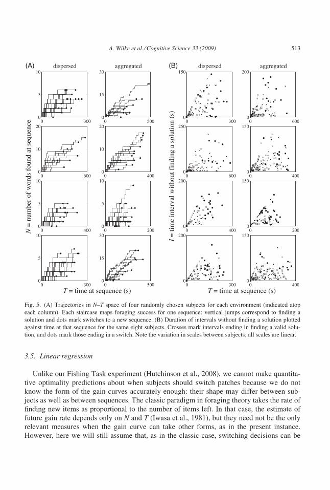
These plots directly translate subjects’ foraging behavior into the way that behavioral

ecologists have depicted the decision rules discussed above (Fig. 2). In Fig. 5A, each line

depicts one visited letter sequence, the vertical steps in these lines show the times at which

subjects entered a valid solution, and the dots mark when subjects hit the switch-sequence

button. For example, in the upper right plot, the topmost line shows a patch where this sub-

ject switched after finding 22 solutions in 481 s. A first inspection of these plots suggests

that the switching points often lie roughly around a straight line with positive slope. This

pattern would arise from a decision rule that, for instance, increments tendency to stay after

each successful capture. Such behavior is appropriate in an environment that is more aggre-

gated than Poisson (Table 1). We cannot tell whether the environments that we constructed

are more or less aggregated than Poisson (and therefore we cannot predict that one of our

environments favors a decremental rule and one an incremental rule), but we can predict

that the switching points in each environment should lie along lines differing in slope. This

is investigated more quantitatively below by fitting regression lines.

The giving-up-time rule (Fig. 2C) utilizes the interval since finding the previous solution.

We can assess whether switching decisions followed this rule by plotting the time intervals Iwithout finding a solution, either until finding the next solution (shown as crosses in

Fig. 5B, which plots I against time T spent at the sequence) or prior to switching (shown as

dots). If people were using a classic giving-up-time rule, then all the dots indicating time

between the final solution and the subsequent switch decision should (a) lie on a horizontal

line parallel to the T-axis and (b) fall consistently above the crosses showing intervals

between successive solutions. However, neither condition appears to hold. Typically, in

about half the sequences seen by a subject, at least one between-solution interval exceeded

the interval preceding switching.


3.5. Linear regression

Unlike our Fishing Task experiment (Hutchinson et al., 2008), we cannot make quantita-

tive optimality predictions about when subjects should switch patches because we do not

know the form of the gain curves accurately enough: their shape may differ between sub-

jects as well as between sequences. The classic paradigm in foraging theory takes the rate of

finding new items as proportional to the number of items left. In that case, the estimate of

future gain rate depends only on N and T (Iwasa et al., 1981), but they need not be the only

relevant measures when the gain curve can take other forms, as in the present instance.

However, here we will still assume that, as in the classic case, switching decisions can be

Fig. 5. (A) Trajectories in N–T space of four randomly chosen subjects for each environment (indicated atop

each column). Each staircase maps foraging success for one sequence: vertical jumps correspond to finding a

solution and dots mark switches to a new sequence. (B) Duration of intervals without finding a solution plotted

against time at that sequence for the same eight subjects. Crosses mark intervals ending in finding a valid solu-

tion, and dots mark those ending in a switch. Note the variation in scales between subjects; all scales are linear.


well summarized by the locus of points in N–T space at which switching has occurred

(Fig. 5A).

To describe this switching function, we fitted a straight regression line to the observed

values of N and T at switching (henceforth NS and TS); we used the function lme() in the

package nlme (version 3.1-66) of the statistical program r (Pinheiro & Bates, 2000; r Deve-

lopment Core Team, 2005). This function fits by maximizing restricted likelihood; for ran-

dom effects we calculated statistical significance by fitting the model with and without the

factor concerned, then computing the likelihood ratio; for fixed effects lme() provides

F-tests conditional on the random-effects variance. We set TS as the dependent variable

(i.e., swapping the axes in Fig. 5A), specified that error increases proportional to the fitted

values (as observed in our data and as expected from the applicability of Weber’s Law to

time intervals), and included subject as a random factor affecting both intercept and slope.

Initial analyses showed that as the experiment progressed subjects tended to switch earlier

for a given value of N, F(1,710) = 49.8, p < .0001, so we also included the time t since the

beginning of the experimental session at which a sequence was encountered.

Our prediction was that subjects facing the more aggregated environment will show

TS-versus-NS slopes that are more positive than subjects facing the more dispersed

environment, because in more aggregated environments finding an item is a more believable

indication that the patch is a very good one, and should thus increase the tendency to

remain. Conversely, in a more dispersed environment, finding an item is of more signifi-

cance in indicating that the number of items remaining in the patch has just got less, so the

tendency to remain may even decrement, generating a more negative or less positive rela-

tionship between TS and NS: see Section 1.1. (Note that considering TS-versus-NS slopes

rather than NS-versus-TS slopes avoids problems caused by the discontinuity in slope when

a line is vertical, as it would be for a fixed-time rule in NS-versus-TS space.) However, it

turned out that the environment had no significant influence on the slope (for the N · envi-

ronment factor, F(1,710) = 1.50, p = .22). The common slope was such that each solution

found would on average delay switching by a further 12.8 s. To give an idea of the goodness

of fit of this model, observed and predicted values differ by a median factor of 15%. If we

fit a line to the data for each individual subject [i.e., subject now a fixed factor interacting

with N; r-function lme() replaced by gls() accordingly], all but five of the 60 slopes are posi-

tive (and none of these five differ significantly from 0, p > .2; approximate t-tests; see Pin-

heiro & Bates, 2000, p. 90).

One possible explanation for these consistently positive slopes in both environments is

that subjects may decide when to switch using initially observable cues of sequence quality,

such as the mean letter frequency, rather than using their success at finding solutions. The

overall positive relationship would then be generated by between-sequence variation—that

is, subjects would stay longer in sequences that they had prejudged as being higher quality,

and consequently they would also generate more solutions for those sequences. Nevertheless

within each sequence it would then probably be optimal for subjects to apply a decremental

rule, ‘‘counting down’’ from expected total number of solutions as each solution is found

(Shaltiel & Ayal, 1998); this would tend to generate a negative relationship between TS and

NS—just the reverse of the incremental rule that adds more time in a patch with every


solution found. To investigate this possibility that looking across sequences masked the

mechanism that was being used within each sequence, we repeated the TS-versus-NS regres-

sion but included sequence as a factor affecting the intercept. This means that we are finding

the mean slope of the switching lines factoring out any influence (on initial tendency to stay)

of the initial quality cues provided by each sequence. Once again, there was no significant

difference in slope between environments, F(1,657) = 1.83, p = .17, and the pooled slope

was positive, confirming that subjects were not using a decremental rule (each solution

delayed switching by 13.5 s; for inclusion of N as a factor, F(1,658) = 200, p < .0001;

observed and predicted values differ by a median factor of 14%).

The fact that the points in the TS-versus-NS plane show a significant relationship does not

necessarily imply that it is N that directly determines TS. The same sort of positive relation-

ship can also be generated if subjects ignore N and T and use only I, the interval since the

previous solution, as a cue for when to switch (Fig. 2C). Both N ⁄ T and 1 ⁄ I can provide esti-

mates of current success rate. To try to disentangle which cues are involved (and whether

people might be using an incremental rule or a modified giving-up-time rule), we performed

the following additional regression analysis.

3.6. Cox proportional hazard model

The Cox proportional hazard model (Cox, 1972) was developed for analyzing survival

data when the outcome of interest is the time to an event (e.g., mortality following different

drug treatments). This method of analysis is now standard in studies of patch leaving in biol-

ogy (Wajnberg, 2006). Although it cannot model the exact form of the decision rules pre-

dicted by optimality theory (because they involve a threshold dependence on N, and this is

usually not consistent for all values of T), it appears able to disentangle which cues were

responsible for producing simulated data generated by such decision rules or by a giving-

up-time rule (Hutchinson et al., 2008).

Whereas the linear regression modeled a deterministic decision rule (i.e., leaving as soon

as a threshold is crossed), the Cox model assumes stochastic decision rules (i.e., various fac-

tors that increase or decrease the probability of patch leaving). Patch-leaving tendency is the

product of a baseline tendency to leave and a combined effect of all the other explanatory

variables zk:

hðT; zÞ ¼ h0ðTÞxi expXMk¼1

bkzkðTÞ !

Here, h is the rate of leaving the patch, h0 is the baseline hazard dependent on the time Tsince the subject entered the patch, xi is a ‘‘frailty’’ factor describing the random variation

between subjects in their tendency to leave (Therneau, Grambsch, & Pankratz, 2003; values

of xi are here assumed to be sampled from a gamma distribution), and bk are the regression

coefficients that give the relative contribution of the M covariates zk. A quantitative measure

of the effect of any particular covariate is then given by the expression exp(bk), the factor


by which the hazard changes with a unit increment of zk. If exp(bk) is >1, an increase in zk

would increase the patch-leaving tendency (i.e., the subject would leave the patch earlier),

while exp(bk) < 1 indicates that the patch-leaving tendency would decrease (i.e., the subject

stays longer at that patch).

We fitted Cox regression using the ‘‘survival’’ (version 2.20) package of the statistical

program r (Therneau, 1999). Data from both environments were analyzed together. We gen-

erated a list of covariates that might affect subjects’ patch-leaving tendency, excluding those

where the direction of causation behind any relationship might be reversed (i.e., with the

strategy affecting the covariate rather than the covariate affecting the strategy; for instance,

the number of solutions found for the preceding sequence might well affect the switching

from the current sequence, but strategies are likely to be consistent between successive

sequences, so any relationship could also be the product of the strategy affecting solutions

found for the preceding sequence; see Hutchinson et al., 2008). Statistical significance of

the frailties and other factors was calculated by analyses of deviance: DD(df) = )2 · (dif-

ference in integrated likelihoods) when adding factors providing df extra degrees of free-

dom; this is distributed as v2(df). We first removed the most nonsignificant (p > .05)

variables progressively, and then tested whether reintroducing each variable was significant

and whether they had interactions with environment and time. At intermediate stages, we

made plots such as those in Fig. 6A–D to examine which simple transformations of the

covariates best generated the linear relationship modeled by Cox regression (see Hutchinson

et al., 2008 for details). Such an approach increases the chance of a Type-I error, but most

terms in our final model are highly significant (Table 2).

How long into the experiment the particular sequence was encountered (t) had a signifi-

cant effect on switching tendency (p = .031), even though we excluded sequences appear-

ing within the first 20 min. Of greater statistical significance were the interactions between

the time of seeing the sequence and two other explanatory variables, mean letter frequency

and whether a solution had yet been found, described further below. In the version of the

model including these interaction terms, the tendency to switch decreased throughout the

experiment (supposing the same values of the other covariates).

We also checked whether a cue to a sequence’s quality could influence switching times,

as predicted by foraging theory. As described above, one such readily assessable cue is the

mean occurrence rate of letters in the sequence, f. This cue turned out to have a strong

negative relationship with the probability of switching sequences (p < .0001; Fig. 6A),

probably because it closely correlates with subjects’ immediate estimations of the number

of available solutions to that sequence (see above). We had expected that the influence of

letter frequency might be higher when first seeing a sequence than later on the same patch

when success rate had provided extra information, but the effect was nonsignificant (not

shown in Table 2; p = .07 based on relationship of Schoenfeld residuals to time T since

the patch was entered: Therneau, 1999, Equation 17) and if anything in the other direction.

Across patches, as the experiment proceeded, subjects put progressively more weight on

mean letter frequency (the ln[f] · t term). For instance, comparing two sequences with let-

ter frequencies at the quartiles of the distribution, subjects were only 1.07 times as likely

after 20 min of the experiment to leave the poor sequence compared to the rich (assuming


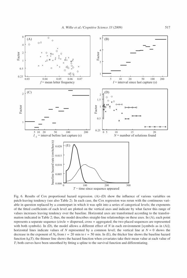
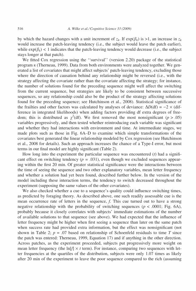
Fig. 6. Results of Cox proportional hazard regression. (A)–(D) show the influence of various variables on

patch-leaving tendency (see also Table 2). In each case, the Cox regression was rerun with the continuous vari-

able in question replaced by a counterpart in which it was split into a series of categorical levels; the exponents

of the fitted coefficients of each level are plotted on the vertical axes and indicate by what factor this range of

values increases leaving tendency over the baseline. Horizontal axes are transformed according to the transfor-

mation indicated in Table 2; thus, the model describes straight-line relationships on these axes. In (A), each point

represents a separate sequence (circle = dispersed, cross = aggregated; the two placed sequences are represented

with both symbols). In (D), the model allows a different effect of N in each environment [symbols as in (A)];

horizontal lines indicate values of N represented by a common level; the vertical line at N = 0 shows the

decrease in the exponent of N0 from t = 20 min to t = 50 min. In (E), the thicker line shows the baseline hazard

function h0(T); the thinner line shows the hazard function when covariates take their mean value at each value of

T; both curves have been smoothed by fitting a spline to the survival function and differentiating.


they had experienced equal success rates on both), whereas after 50 min the factor had

increased to 2.6.

The interval I since entering the previous correct solution (or, if no solution had been

found, since the sequence first appeared) was positively associated with the probability of

switching (p < .0001; Fig. 6B). We also tried including the interval since the previous word

entry whether correct or incorrect, but this was a less good predictor than I and, in combina-

tion, did not add significantly to the explanatory power (DD[1] = 1.6, p = .21). But I)1, the

interval preceding the previous correct solution, did also significantly increase the probabil-

ity of switching (p = .0001; Fig. 6C). The effects of I and I)1 were consistent over the

course of the experiment (for ln[I] · t, DD[1] = 0.11, p = .74; for �I)1 · t, DD[1]= 0.20,

p = .65). Switching tendency was a factor of 2.5 higher after 30 s since finding a solution

than after 5 s. The effect was smaller for the preceding interval: when I)1 was 30 s, switch-

ing tendency was 1.25 times higher than when I)1 was 5 s. There was no indication of a

nonadditive interaction between the effects of I and I)1 (e.g., an increase in interval duration

from I)1 to I triggering leaving).

In order to consider I)1 without ignoring periods before any solutions were found, it was

necessary to include a second variable N0 in addition to I)1 (with N0 = 1 and I)1 = 0 before

the first solution for a sequence was found, otherwise N0 = 0). Through the course of the

experiment, the coefficient (and direction of effect) of N0 changed significantly (N0 · t term,

p < .0001): 20 min into the experiment subjects were 2.3 times keener to switch before they

had found their first solution than they were after (assuming other covariates were identical),

whereas 50 min into the experiment they were 2.1 times keener to switch after finding their

first solution than before.

There was a marginally significant difference between environments in the influence of N(DD[1] = 3.7, p = .053). Whereas in the aggregated environment increasing N significantly

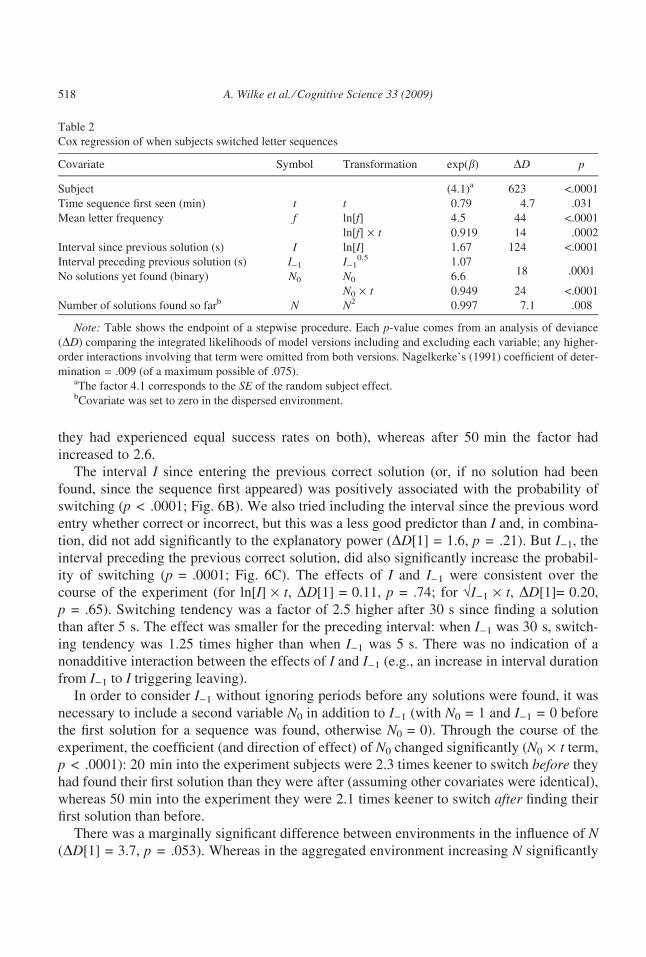
Table 2

Cox regression of when subjects switched letter sequences

Covariate Symbol Transformation exp(b) DD p

Subject (4.1)a 623 <.0001

Time sequence first seen (min) t t 0.79 4.7 .031

Mean letter frequency f ln[f] 4.5 44 <.0001

ln[f] · t 0.919 14 .0002

Interval since previous solution (s) I ln[I] 1.67 124 <.0001

Interval preceding previous solution (s) I)1 I)10.5 1.07

18 .0001No solutions yet found (binary) N0 N0 6.6

N0 · t 0.949 24 <.0001

Number of solutions found so farb N N2 0.997 7.1 .008

Note: Table shows the endpoint of a stepwise procedure. Each p-value comes from an analysis of deviance

(DD) comparing the integrated likelihoods of model versions including and excluding each variable; any higher-

order interactions involving that term were omitted from both versions. Nagelkerke’s (1991) coefficient of deter-

mination = .009 (of a maximum possible of .075).aThe factor 4.1 corresponds to the SE of the random subject effect.bCovariate was set to zero in the dispersed environment.


decreased leaving tendency (p = .008), there was no such effect in the dispersed environ-

ment (DD[1] = 0.4, p = .52; Fig. 6D). This fits a main prediction from optimality theory

that in a more aggregated environment captures should have a more incremental (or less

decremental) effect on tendency to stay (hence the more negative influence of N on leaving

tendency). However, note that the effect size is quite small: in the aggregated environment,

finding eight solutions decreased leaving tendency by a factor of only 0.80 compared with

having found just one solution. None of the other variables in Table 2 showed significant

interactions with environment (all p > .10) and nor did the frailties differ between environ-

ments, t(55) = 0.94, p = .35.

The form of the baseline hazard function h0(T) shows a maximum 50 s after a sequence is

first inspected (thick line in Fig. 6E), so that beyond 50 s, if nothing else were to change, sub-

jects would become progressively less likely to switch. This decline still exists but is delayed

if we take into account the changing mean values of the covariates (thinner line in Fig. 6E).

However, the decline is potentially an artifact generated by nonmultiplicative heterogeneity

in the form of the hazard function.

3.7. Analyses of placed sequences

Across subjects, there was no difference between environment in median NS, TS, or IS

for either the high- or low-difficulty placed sequences (all six p > .18; Mann–Whitney), but

this is not surprising given the considerable intersubject variation in skill and persistence. A

more revealing procedure is to test how much longer each subject spent on the second, eas-

ier sequence than on the first, and compare this between environments. Across both environ-

ments, 40 out of 60 subjects spent longer on the easier sequence (significantly different

from a 1:1 ratio, p = .013), with a median difference of 20 s. We expected subjects to be

more willing in the aggregated environment to increase residence time when a sequence

seemed easier, but there was no such difference in the median increase between environ-

ments, Mann–Whitney, U(30,30) = 912, p = .98. This is further evidence that subjects did

not seem sensitive to the difference in environment structure that we created.

In 44 out of 60 subjects, giving-up time IS was shorter with the easier sequence. This pro-

portion is significantly different from 1:1 (p < .0001). This emphasizes again that subjects

cannot be using a classic giving-up-time rule, although the result is not incompatible with

other more complex I-dependent rules.

3.8. Self-reports

After the main experiment, we asked all 60 subjects to rate how often they used each of

the three cues, N, T, and I, in determining their switching decisions (Table 3). For all three

cues, the modal response was 3 on the four-point scale (i.e., ‘‘often’’), so it is more reveal-

ing to compare within subjects whether their rating of one cue was higher than that of

another. Comparing ratings of the use of I and N, the value for I was higher in 28 subjects,

and lower in 10 subjects, which is significantly different from 1:1 (p = .005). Comparing

ratings of the use of I and T, the value for I was higher in 27 subjects, and lower in 12


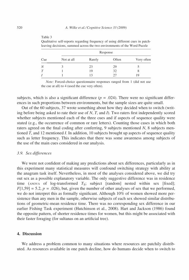
subjects, which is also a significant difference (p = .024). There were no significant differ-

ences in such proportions between environments, but the sample sizes are quite small.

Out of the 60 subjects, 37 wrote something about how they decided when to switch (writ-

ing before being asked to rate their use of N, T, and I). Two raters first independently scored

whether subjects mentioned each of the three cues and if aspects of sequence quality were

stated (e.g., the occurrence of common or rare letters). Counting those cases in which both

raters agreed on the final coding after conferring, 9 subjects mentioned N, 8 subjects men-

tioned T, and 12 mentioned I. In addition, 10 subjects brought up aspects of sequence quality

such as letter frequency. This indicates that there was some awareness among subjects of

the use of the main cues considered in our analysis.

3.9. Sex differences

We were not confident of making any predictions about sex differences, particularly as in

this experiment many statistical measures will confound switching strategy with ability at

the anagram task itself. Nevertheless, in most of the analyses considered above, we did try

out sex as a possible explanatory variable. The only suggestive difference was in residence

time (anova of log-transformed TS; subject [random] nested within sex [fixed];

F[1,59] = 5.2, p = .026), but, given the number of other analyses of sex that we performed,

we do not interpret this as formally significant. Although 10% of women showed more per-

sistence than any men in the sample, otherwise subjects of each sex showed similar distribu-

tions of geometric-mean residence time. There was no corresponding sex difference in our

earlier Fishing Task experiment (Hutchinson et al., 2008). Hart and Jackson (1986) found

the opposite pattern, of shorter residence times for women, but this might be associated with

their faster foraging (for sultanas on an artificial tree).

4. Discussion

We address a problem common to many situations where resources are patchily distrib-

uted. As resources available in one patch decline, how do humans decide when to switch to

Table 3

Qualitative self-reports regarding frequency of using different cues in patch-

leaving decisions, summed across the two environments of the Word Puzzle

Cue

Response

Not at all Rarely Often Very often

N 3 23 29 5

T 1 19 32 8

I 1 13 27 19

Note: Forced-choice questionnaire responses ranged from 1 (did not use

the cue at all) to 4 (used the cue very often).


a fresh patch? Our earlier research used a computer game to investigate when people switch

from one pond depleted of fish to another undepleted one, comparing behavior with rules

from theoretical work on animal foraging (the Fishing Task; see Hutchinson et al., 2008).

Here we test whether similar mechanisms are used in a puzzle task with a similar patch

structure, but in which the items sought are internally generated solutions (i.e., words con-

structed from provided letter sequences) rather than items in the external environment.

4.1. The cues that influence switching

To facilitate comparison with the Fishing Task, where there were no cues to the quality

of each pond when initially encountered, we had attempted to make each letter sequence

appear at first glance equally easy (equal length, same ratio of vowels to consonants, rarest

letters omitted). Despite this, the mean rate of occurrence of the letters in German, averaged

over all letters in the sequence, was a good predictor of the number of solutions available.

Mean letter frequency also predicted both subjects’ snap estimates of number of solutions

and their willingness to switch sequences, so probably letter frequency is one cue influenc-

ing the switching decision. While these correlations could be due to some confounding

aspect of sequence quality, several self-reports spontaneously mentioned that the presence

of particular common or rare letters influenced persistence.

Similarly, Pirolli (2005, 2007) explained persistence in exploring Websites in terms of

proximal cues (which he termed information scent) to the quality of items in a patch. How-

ever, that search situation was rather different from ours in that some items (Websites) were

more valuable than others, and these were the items chosen first via the indications of infor-

mation scent. Thus for Web-search patches, it was probably the declining quality of the suc-

cessive individual items rather than the directly estimated initial quality of the patch itself

that determined when people switched.

In the Fishing Task, the most important cues that people used to decide when to switch

were cues to patch quality provided by recent foraging success, specifically the time since

finding the previous solution (I) and the interval between finding the previous two solutions

(I)1). We found strong effects of both of these cues in the Word Puzzle Task as well. Their

importance compared to other cues was supported by subjects’ self-reports. Note that in nei-

ther experiment did the subjects always switch once a threshold time without a success had

been exceeded, so the classic giving-up-time rule is too simplistic to account for our sub-

jects’ behavior. Rather, the Cox regression suggested a quantitative influence of I and I)1 on

the tendency to switch. In part, this quantitative effect may reflect averaging over subjects,

and we cannot yet say precisely how these interval cues are utilized.

It might seem unsurprising that a long wait for the next solution would trigger switch-

ing—mounting impatience seems a natural call to action. However, in the idealized patch-

leaving scenario modeled by behavioral ecologists, an organism would be better off to

ignore this information if instead proper use were made of two other cues: the total number

of solutions found (N) and the total time spent (T) so far in the current patch. Together these

yield a longer-term measure of success rate. Unlike in the Fishing Task, where there was no

evidence of an effect of N, in the Word Puzzle Task tendency to switch did significantly


decrease as N increased, although the effect was weak and apparent only in the aggregated

environment.

One consequence of the dependency of switching tendency on I and I)1 is the positive

relationship that we observed between the number of solutions NS found for a sequence and

the time TS spent on that sequence. The pattern is highly consistent across subjects. The

positive direction of this relationship is adaptive in an aggregated environment in which the

quality of sequences is unpredictable (specifically, less predictable than if posterior proba-

bilities of qualities followed a Poisson distribution). However, if sequence quality is some-

what (but not completely) predictable we expect a negative relationship, generated by

decreasing the tendency to stay with each new solution found. The fact that subjects have

access to, and apparently use, the reliable letter-frequency cue to quality would imply that

sequence quality is rather predictable. Thus, the positive NS-versus-TS slopes that subjects

actually generate may well be nonadaptive in this particular task.

Some comparison is due with the results of Payne et al. (2007) who also assessed the cues

that subjects used to switch between anagram tasks. Their experiment differed in returns to

the same patch being allowed, the number of patches being restricted to two, and in not

allowing the subjects much time to learn about the environment (10 or 15 min duration).

Nevertheless, it is not unreasonable that in both situations subjects might use similar ways

to assess future returns in the current patch, which is one half of the equation about when to

switch. Like us, Payne et al. (2007) observed behavior inconsistent with a fixed-T or a fixed-

N rule, or with a classic giving-up-time rule (as in our experiment, visits often had an inter-

solution interval longer than IS). Instead they fitted a model based on a combination of Tand N, with the fitted coefficient of N positive (i.e., an incremental rule). Payne et al. (2007)

were struck that giving-up times were longer in the harder patches (also evident in our data;

48 of our 60 subjects showed a negative rS between IS and number of solutions in our word

list), and by the ability of their model to generate such a pattern. However, this pattern is a

natural outcome of many rules incorporating an influence of T or N: all it implies is that sub-

jects put some reliance on prior expectations about sequence difficulty, so that they do not

fully believe that gain rate has declined so soon (in terms of T or N) in a poor patch, and

consequently persist (whereas the same gain rate in a good patch would arise later). A vari-

ety of rules have this property, and Payne et al. do not assess whether a rule involving I and

T, for instance, could explain their data better. Nor did they investigate the influence of prior

assessment of sequence quality (e.g., from letter frequency).

4.2. The (absent) effect of environment structure

Predictability of sequence quality depends not only on the reliability of the immediate

cues to quality but also on how much sequence quality varies across the environment

encountered. In the Word Puzzle Task, sequence quality and the form of the gain curve

depend on each individual subject’s knowledge and abilities, so it is difficult to quantify the

variation of sequence quality. Instead we manipulated this variation to create environments

differing in their degree of aggregation ⁄ dispersion. This manipulation made very little dif-

ference either to the relationship between NS and TS, or to the difference in time spent in the


easy and difficult placed sequences, or to the quantitative influences of letter frequency,

I, and I)1 on switching tendency. The only between-environment difference was a margin-

ally significant difference in whether N was incorporated in the decision; the difference was

in the predicted direction but minor in effect. One possible reason for this lack of difference

between the two environments is that the letter-frequency cue might have made both simi-

larly predictable, although we would expect some residual difference given that letter fre-

quency is an imperfect guide to ease of solutions. We also found this surprising absence of

influence of environment structure in the Fishing Task, where we established precise varia-

tion in resources across patches without any immediate cues to quality. For that task, we

could make quantitative predictions that the form of the switching policy should have chan-

ged dramatically given the large differences in patch-quality variation—but it did not.

4.3. Why apply I-dependent decision rules independent of the environment?

Humans are intelligent animals and well adapted in other ways to cope with a great diver-

sity of food types; some of these foods are liable to be dispersed more evenly across suitable

sites than others. So we expected humans to be sensitive to this aspect of the environment,

even though the few tests of such sensitivity in other animals have not clearly supported it

(reviewed in Hutchinson et al., 2008).

One class of explanation for the insensitivity we instead found is that reliably assessing

the variation of patch quality in the environment requires visiting a number of patches, espe-

cially if patch quality is not immediately recognizable but can only be imperfectly estimated

from the foraging success experienced before switching. Consequently, in unfamiliar situa-

tions such as in our experiments (at least as long as they remain unfamiliar), it may pay to

use a rule that is robust across a range of environments. Rules based on intervals since the

previous capture can have this property (Hutchinson et al., 2008) and they are also robust to

unexpected deteriorations of a patch (e.g., if all prey hide).

Another related adaptive explanation is that these rules perform particularly well with

aggregated distributions, and it has been argued that aggregated distributions of prey items

are more common in nature than dispersed distributions (e.g., Taylor, Woiwod, & Perry,

1978). Plants and animals rarely, if ever, are distributed in a purely random manner in their

natural environment, partly because individual organisms are not independent from one

another: whereas mutual attraction leads to aggregation for some species, mutual repulsion

leads to regularity (dispersed environments) in other species (Taylor, 1961). But these devi-

ations from randomness may more often be in the direction of aggregation as it can offer

considerable ecological benefits (e.g., Krause & Ruxton, 2002). Such advantages can arise

through responses to physical environments (e.g., resource availability or light), reproduc-

tive behavior (e.g., clumped placement of offspring), mutual attraction to other individuals

of the same species (e.g., for mating opportunities), interactions with other species (e.g., par-

asite or predator avoidance), or group foraging behavior (e.g., capturing prey types impossi-

ble for a single individual to catch). As humans have been hunters and gatherers for

about 99% of our species’ history (Tooby & DeVore, 1987), it could well be that our

(evolved) psychology is adapted to assume such aggregated resource distributions as the


environmental default, an assumption that would have offered a selective advantage under

ancestral conditions. However, whether resources are aggregated in space (i.e., are patchy)

is a related but distinct issue to whether the distribution of items across patches is aggre-

gated (e.g., suppose that fish form shoals—patches—but all are of uniform size): much of

the evidence for the predominance of aggregated distributions is based on counts per ran-

dom quadrat and thus might reflect merely patchiness itself (Rodrıgues-Girones & Vasquez,

1997). So more work would be required to establish that foods consumed by hunter-gather-

ers are most commonly aggregated in distribution across what they might perceive as

suitable patches worth searching.

But what really matters in this context is the remaining uncertainty in patch quality once

immediate cues to quality have been assessed. It is probably often the case in foraging situa-

tions that there are immediate cues to patch quality that considerably reduce this uncertainty

even if prey are aggregated in a minority of patches, and foragers ought to be able to learn

quite readily through experience which cues can make their immediate estimates of patch

quality reliable. Such a cue was available and was utilized in the Word Puzzle Task, thus

making patch quality more predictable. Therefore, the switching rule’s consistent depen-

dence on I and I)1 does not seem adequately explained as an adaptive best-guess that the

environment is aggregated, as the evident predictability of patch quality in this situation

makes other rules superior.

Another sort of explanation for the rule consistency across environments is that perhaps

humans use general search processes that are subject to carry-over influences from one

search task to another, limiting their ability to adapt to different environments. Along these

lines, Hills, Todd, and Goldstone (2007) and Hills et al. (2008b) showed that behavioral

search tendencies can be primed within individuals who perform a succession of search

tasks. Subjects who first perform a spatial search task in a patchy resource environment later

behave as if resources are also more densely clumped in an abstract cognitive search task

(very similar to the Word Puzzle Task used here). These results are in accordance with the

claim that much of human goal-directed cognition can be understood as a descendent of

animal foraging behavior (see Hills, 2006). However, this explanation depends on subjects

having been primed by earlier encounters with aggregated environments.

A similar but broader explanation proposes that our subjects are applying a simple gen-

eral-purpose learning rule that is adaptive in other contexts beyond search (as discussed in

Hutchinson et al., 2008). In the context of a simultaneous choice between two stable

options, it is sensible that humans and other animals prefer the one that provides shorter

delays to reinforcement. If they attempt to apply this principle to the two options of switch-

ing and staying, I and I)1 might reasonably provide the estimate of future delays to rein-

forcement under the staying option (while experience of travel time between patches and of

the subsequent wait till the first capture at a new patch provides an estimate for the switch-

ing option). The win-stay behavior that this general rule produces is adaptive in many con-

texts, but not in the situation as here of depleting patches with good prior knowledge of how

many items the patch contains, when at some point win-shift behavior instead becomes

appropriate. Thus, this learning rule would lead subjects to rely on I and I)1 and miss the

usefulness of N and T.


4.4. Similarities and differences between strategies in the Fishing Task and Word PuzzleTask

The idea that patch-switching behavior in both of our experiments is driven by a general

learning rule evolved for other contexts must be compared against other possibilities,

including that people have a range of domain-specific patch-switching rules (but maybe

failed to deploy them in our experiments), and that people have a more general patch-

switching rule that can be modified from environment to environment. This comparison will

require more experimental data, and the results will be relevant to the ongoing discussion

regarding the extent of the modular nature of the human mind (Barrett & Kurzban, 2006).

However, our two experiments already establish that similar rules dependent on I and I)1

are used in two rather different patch-switching contexts. With the Fishing Task we made it

evident to subjects that the experimental problem was analogous to a real foraging task,

whereas in the Word Puzzle Task there were no such obvious connections. In the Fishing

Task, items had to be found in the external environment, which required minimal cognitive

effort since the fish were usually not difficult to spot once they appeared. With the Word

Puzzle, solutions had to be generated internally with considerable cognitive effort, probably

by a mixture of generating bigrams or syllables out of the provided letter sequence and

searching in memory for words containing such syllables (Hills, Goldstone, & Todd,

2008a).

In addition, the strategies applied in the two experiments were similar in generating

patch-residence times that were considerably longer than optimal—people switched too

late. This is a pattern common also to most studies of animal patch switching (Nonacs,

2001) and to a study in which humans foraged for sultanas on artificial trees (Hart &

Jackson, 1986). Part of the reason could be that foragers allow for risks associated with

moving between patches, which though not present in the experimental setting often may

be present in nature; such risks would dictate staying longer in each patch. Hutchinson

et al. (2008) also consider a different explanation based on subjects short-sightedly mini-

mizing delay to the very next item alone and thereby preferring the next item in the

same patch rather than in a new one, thus ignoring the extra advantage from switching

that comes from the succession of short intercapture intervals following the first capture

on a fresh patch.

In one conspicuous respect, behavior in the Fishing Task differed from that in the

Word Puzzle: in the former, subjects often (20% of patches) switched within 4 s of find-

ing a fish, with the tendency to do so stimulated by long waits before that fish (I)1) and

the preceding one. One explanation that Hutchinson et al. (2008) proposed for this non-

adaptive behavior was the so-called Concorde Effect or sunk-cost fallacy (Arkes &

Ayton, 1999): during a long wait subjects may have decided to switch directly after the

next capture, rather than immediately, through an illogical reluctance not to ‘‘waste’’ the

time already spent waiting. An alternative explanation is that switching straight after a

capture can be optimal in the common natural situation of an overdispersed timing of

captures, for instance, when a capture makes neighboring prey hide or when prey are

spread out within a patch. In contrast, the phenomenon of switching straight after a


capture was almost absent in the Word Puzzle (only 3.5% switches within 4 s of a cap-

ture). We propose that the reason is that finding one solution tends to provide ideas for

another, so that with this task the timing of captures is aggregated within a patch, rather

than overdispersed. Thus, this aspect of switching strategy appears responsive to relevant

differences in the environment. It is puzzling, therefore, why Payne et al. (2007) did

often observe switching directly after finding a solution in an anagram task very similar

to ours, especially as they took fewer precautions to avoid clustering of solutions; they

related the phenomenon to a general tendency to switch tasks after subgoal completion,

so as to avoid disturbing interruptions.

4.5. Further directions

Given the considerable intersubject variation revealed in both of our experiments, future

studies might profitably use within-subject designs to address why subjects are rather insen-

sitive to environmental variation. To what extent do people adhere to previously used deci-

sion rules when the environment they are in changes so that a different patch-leaving rule

becomes ecologically rational? For instance, in a similar experiment involving an external

foraging task (Mata, Wilke, & Czienskowski, unpublished data), when key environmental

parameters—such as the travel time between resource patches—were changed, both youn-

ger and older adults were able to adapt their strategy parameters and to follow explicit strat-

egy instructions. But on the other hand, Hills et al.’s (2008b) results on priming between

search tasks suggest that even considerable task-environment changes may not lead to

changes in behavior.

We believe that there are many contexts in everyday life where patch structure gen-

erates a problem analogous to the Word Puzzle and Fishing Task experiments, which

may be solved by similar strategies—whether or not those strategies are specific to

patch-switching. The patches might be real locations such as shops or towns, or virtual

locations, as Pirolli et al. have considered with the search for information across Web

pages. These patches may be renewing rather than depleting and may be foraged by

cooperating groups instead of competing individuals (Giraldeau & Caraco, 2000). Or

the patches might be a set of different tasks (Payne et al., 2007); for instance, consider

how one decides when to stop tidying the house and start cutting firewood or go off

shopping. In all of these cases, the patches are defined by the external environment

(even if the items in the patch are then sought internally, as in the Word Puzzle Task);

but patches can also be internally defined and cognitively constructed. For instance, in

the Word Puzzle Task subjects could decide to try to think first of words starting with

one letter from the sequence, then words starting with another letter, thereby creating

an additional internal level of patch-leaving decisions. This patchiness may be a gen-

eral feature of accessing memory using a succession of association cues, one after

another. Further methodologies, along with refinements in the methodology reported

here, will allow exploration of these various different patch-foraging contexts, including

possible hierarchical patch structures, and of the decision rules humans use to respond

to them.


Acknowledgments

We are very grateful to Gregor Caregnato, Julia Ksenski, and Julian Marewski for their

help in conducting this research, and to Clark Barrett, Willem Frankenhuis, Rui Mata,

Stephen Payne, Peter Pirolli, and an anonymous reviewer for their thoughtful comments on

the manuscript. Florian Richter (Technical University of Chemnitz) and Stefan Bordag

(University of Leipzig) provided generous help in compiling word lists. The first author was

supported by Research Fellowship WI 3215 ⁄ 1-1 from the German Research Foundation

(DFG) and the Owen F. Aldis Scholarship Fund from the International Society for Human

Ethology (ISHE). The research was approved by the Ethics Committee of the Max Planck

Institute for Human Development.

References

van Alphen, J. J. M., Bernstein, C., & Driessen, G. (2003). Information acquisition and time allocation in insect

parasitoids. Trends in Ecology and Evolution, 18, 81–87.

Arkes, H. R., & Ayton, P. (1999). The sunk cost and Concorde effects: Are humans less rational than lower ani-

mals? Psychological Bulletin, 125, 591–600.

Barrett, H. C., & Kurzban, R. (2006). Modularity in cognition: Framing the debate. Psychological Review, 113,

628–647.

Bauer, F. L. (2000). Entzifferte Geheimnisse. Berlin: Springer.

Bell, W. J. (1991). Searching behaviour: The behavioural ecology of finding resources. New York: Chapman

and Hall.

Burger, O., Hamilton, M. J., & Walker, R. (2005). The prey as patch model: Optimal handling of resources with

diminishing returns. Journal of Archaeological Science, 32, 1147–1158.

Charnov, E. L. (1976). Optimal foraging, the Marginal Value Theorem. Theoretical Population Biology, 9, 129–

136.

Cox, D. R. (1972). Regression models and life tables. Biometrics, 38, 67–77.

Czienskowski, U. (2005a). WordListGenerator [computer software]. Berlin: Max Planck Institute for Human

Development.

Czienskowski, U. (2005b). The Word Puzzle experiment [computer software]. Berlin: Max Planck Institute for

Human Development.

Driessen, G., & Bernstein, C. (1999). Patch departure mechanisms and optimal host exploitation in an insect par-

asitoid. Journal of Animal Ecology, 68, 445–459.

Gigerenzer, G., Todd, P. M., & the ABC Research Group (1999). Simple heuristics that make us smart. New

York: Oxford University Press.

Gilchrist, I. D., North, A., & Hood, B. (2001). Is visual search really like foraging? Perception, 30,

1459–1464.

Giraldeau, L.-A., & Caraco, T. (2000). Social foraging theory. Princeton, NJ: Princeton University Press.

Goldstone, R. L., & Ashpole, B. C. (2004). Human foraging behavior in a virtual environment. PsychonomicBulletin and Review, 11, 508–514.

Goldstone, R. L., Ashpole, B. C., & Roberts, M. E. (2005). Knowledge of resources and competitors in human

foraging. Psychonomic Bulletin and Review, 12, 81–87.

Hart, P. J. B., & Jackson, P. H. (1986). The influence of sex, patch quality, and travel time on foraging decisions

by young adult Homo sapiens L. Ethology and Sociobiology, 7, 71–89.

Hills, T. T. (2006). Animal foraging and the evolution of goal-directed cognition. Cognitive Science, 30, 3–41.


Hills, T. T., Todd, P. M., & Goldstone, R. L. (2007). Priming and conservation between spatial and cognitive

search. In D. S. McNamara & J. G. Trafton (Eds), Proceedings of the twenty-ninth annual conference of theCognitive Science Society (pp. 359–364). Mahwah, NJ: Erlbaum.

Hills, T. T., Goldstone, R. L., & Todd, P. M. (2008a). Evidence for generalized cognitive search processes at

multiple levels in a hierarchical problem solving task. In B. C. Love, K. McRae & V. M. Sloutsky (Eds),

Proceedings of the thirtieth annual conference of the Cognitive Science Society (p. 1656). Mahwah, NJ:

Erlbaum.

Hills, T. T., Todd, P. M., & Goldstone, R. L. (2008b). Search in internal and external spaces: Evidence for gener-

alized cognitive search processes. Psychological Science, 19, 802–808.

Hutchinson, J. M. C., Wilke, A., & Todd, P. M. (2008). Patch leaving in humans: Can a generalist adapt its rules

to dispersal of items across patches? Animal Behaviour, 75, 1331–1349.

Iwasa, Y., Higashi, M., & Yamamura, N. (1981). Prey distribution as a factor determining the choice of optimal

foraging strategy. American Naturalist, 117, 710–723.

Kelly, R. L. (1995). The foraging spectrum. Washington, DC: Smithsonian Institution Press.

Klein, R. M. (2000). Inhibition of return. Trends in Cognitive Sciences, 4, 138–147.

Krause, J., & Ruxton, G. D. (2002). Living in groups. Oxford, England: Oxford University Press.

Krebs, J. R., Ryan, J. C., & Charnov, E. L. (1974). Hunting by expectation or optimal foraging? A study of patch

use by chickadees. Animal Behaviour, 22, 953–964.

Livoreil, B., & Giraldeau, L.-A. (1997). Patch departure decisions by spice finches foraging singly or in groups.

Animal Behaviour, 54, 967–977.

McNamara, J. M. (1982). Optimal patch use in a stochastic environment. Theoretical Population Biology, 21,

269–288.

McNamara, J. M., & Houston, A. I. (1985). Optimal foraging and learning. Journal of Theoretical Biology, 117,

231–249.

Metcalfe, D., & Barlow, K. R. (1992). A model for exploring the optimal trade-off between field processing and

transport. American Anthropologist, 94, 340–356.

Nagelkerke, N. J. D. (1991). A note on a general definition of the coefficient of determination. Biometrika, 78,

691–692.

Nonacs, P. (2001). State dependent behavior and the marginal value theorem. Behavioral Ecology, 12, 71–83.

Payne, S. J., Duggan, G. B., & Neth, H. (2007). Discretionary task interleaving: Heuristics for time allocation in

cognitive foraging. Journal of Experimental Psychology: General, 136, 370–388.

Pinheiro, J. C., & Bates, D. M. (2000). Mixed-effects models in S and S-Plus. New York: Springer.

Pirolli, P. (2005). Rational analyses of information foraging on the Web. Cognitive Science, 29, 343–373.

Pirolli, P. (2007). Information foraging theory: Adaptive interaction with information. New York: Oxford

University Press.

Pirolli, P., & Card, S. (1997). The evolutionary ecology of information foraging. (Tech. Rep. No. UIR-R97-01).

Palo Alto, CA: Xerox PARC.

Pirolli, P., & Card, S. (1999). Information foraging. Psychological Review, 106, 643–675.

r Development Core Team (2005). r: A language and environment for statistical computing. Vienna, r Founda-

tion for Statistical Computing.

Rajala, A. K., & Hantula, D. A. (2000). Towards a behavioral ecology of consumption: Delay-reduction effects

on foraging in a simulated Internet mall. Managerial and Decision Economics, 21, 145–158.

Rodrıgues-Girones, M. A., & Vasquez, R. A. (1997). Density-dependent patch exploitation and acquisition of

environmental information. Theoretical Population Biology, 52, 32–42.

Rogers, R. D., & Monsell, S. (1995). Costs of a predictable switch between simple cognitive tasks. Journal ofExperimental Psychology: General, 124, 207–231.

Sandstrom, P. E. (1994). An optimal foraging approach to information seeking and use. Library Quarterly, 64,

414–449.

Sandstrom, P. E. (1999). Scholars as subsistence foragers. Bulletin of the American Society for InformationScience, 25, 17–20.


Shaltiel, L., & Ayal, Y. (1998). The use of kairomones for foraging decisions by an aphid parasitoid in small

host aggregations. Ecological Entomology, 23, 319–329.

Smith, C. L., & Hantula, D. A. (2003). Pricing effects on foraging in a simulated Internet shopping mall. Journalof Economic Psychology, 24, 653–674.

Stephens, D. W., & Krebs, J. R. (1986). Foraging theory. Princeton, NJ: Princeton University Press.

Taylor, L. R. (1961). Aggregation, variance and the mean. Nature, 189, 732–735.

Taylor, L. R., Woiwod, I. P., & Perry, J. N. (1978). The density-dependence of spatial behaviour and the rarity

of randomness. Journal of Animal Ecology, 47, 383–406.

Therneau, T. M. (1999). A package for survival analysis in S. Technical Report Mayo Foundation [accessed on

February 28, 2009]. Available at http://mayoresearch.mayo.edu/mayo/research/biostat/upload/survival.pdf

Therneau, T. M., Grambsch, P. M., & Pankratz, V. S. (2003). Penalized survival models and frailty. Journal ofComputational and Graphical Statistics, 12, 156–175.

Todd, P. M., & Gigerenzer, G. (2007). Environments that make us smart: Ecological rationality. CurrentDirections in Psychological Science, 16, 167–171.

Tooby, J., & DeVore, I. (1987). The reconstruction of hominid behavioral evolution through strategic modeling.

In W. G. Kinsey (Ed.), The evolution of primate behavior: Primate models (pp. 183–237). New York: New

York Suny University Press.

Waage, J. K. (1979). Foraging for patchily-distributed hosts by the parasitoid, Nemeritis canescens. Journal ofAnimal Ecology, 48, 353–371.

Wajnberg, E. (2006). Time allocation strategies in insect parasitoids: From ultimate predictions to proximate

behavioral mechanisms. Behavioral Ecology and Sociobiology, 60, 589–611.

Wajnberg, E., Fauvegue, X., & Pons, O. (2000). Patch leaving decision rules and the marginal value theorem:

An experimental analysis and a simulation model. Behavioral Ecology, 11, 577–586.

Wajnberg, E., Gonsard, P.-A., Tabone, E., Curty, C., Lezcano, N., & Colazza, S. (2003). A comparative analysis

of patch-leaving decision rules in a parasitoid family. Journal of Animal Ecology, 72, 618–626.

Wanchisen, B. A., Tatham, T. A., & Hineline, P. N. (1992). Human choice in ‘‘counterintuitive’’ situations:

Fixed- versus progressive-ratio schedules. Journal of the Experimental Analysis of Behavior, 58, 67–85.

Wang, Z., Busemeyer, J. R., & Lang, A. (2006). Grazing or staying tuned: A stochastic dynamic model of chan-

nel changing behavior. In R. Sun (Ed.), Proceedings of the twenty-eighth annual conference of the CognitiveScience Society (pp. 870–875). Mahwah, NJ: Erlbaum.

Wilke, A. (2006). Evolved responses to an uncertain world [accessed on February 28, 2009]. PhD Thesis, Free

University of Berlin. Available at http://www.diss.fu-berlin.de/2006/14/indexe.html

Wilke, A., Hutchinson, J. M. C., & Todd, P. M. (2004). Testing simple rules for human foraging in patchy envi-

ronments. In K. Forbes, D. Genter & T. Regier (Eds), Proceedings of the twenty-sixth annual conference ofthe Cognitive Science Society (p. 1656). Mahwah, NJ: Erlbaum.

Winterhalder, B., & Smith, E. A. (1981). Hunter-gatherer foraging strategies: Ethnographic and archaeologicalanalyses. Chicago: University of Chicago Press.


Documents

Fishing for the Right Words: Decision Rules for Human