Embed Size (px)
Citation preview

FISCAL POLICY IN SOUTH AFRICA: AN INTERTEMPORAL
CGE ANALYSIS
Margaret Chitiga, Ramos Mabugu, Hélène Maisonnave and Véronique Robichaud
For an Equitable Sharing of National Revenue

OUTLINE OF THE PRESENTATION
• Aims and Objectives• Methodology• Results• Conclusion
2Workshop Name
Date 2011

AIMS AND OBJECTIVES
• New Growth Plan involves accelerated investment program in social and economic infrastructure and general government spending
• These expansionary fiscal strategies raise a number of critical policy questions:– composition of spending – financing strategies (taxation or increased debt)
• How would these policies and their financing affect the South African economy in the short, medium and long run?
• CGE analysis in a forward-looking perspective3
Workshop NameDate 2011

METHODOLOGY - JUSTIFICATION
• CGE analysis that allows taking into account all the linkages between productive sectors, demand, international trade and macroeconomic constraints
• As measures are known in advance, a forward-looking behaviour (for firms and households) is more suitable
• Impact of infrastructure on economic growth is taken into account
4Workshop Name
Date 2011

METHODOLOGY - OVERVIEW
• Multi-sector analysis (19 industries and commodities)
• Intertemporal framework: all current and future prices are known and affect firms investment decision and households consumption pattern
• Taxation options: many tax instruments are explicitly modelled to allow for a wide variety of policy responses
5Workshop Name
Date 2011

METHODOLOGY - FIRMS
• Representative firm in each industry that combines labour, capital and intermediate inputs to produce composite commodities that can be sold either locally or exported.
• Constant returns to scale technology • Competitive environment in the good markets, as
well as in factor markets.
6Workshop Name
Date 2011

METHODOLOGY - FIRMS
• Nested structure:
7Workshop Name
Date 2011
Total output
Value added Total intermediate cons.
Capital Labour Int. cons. by commodity
Leontief
LeontiefCES

METHODOLOGY - FIRMS
• Nested structure:
8Workshop Name
Date 2011
Total output
Value added Total intermediate cons.
Capital Labour Int. cons. by commodity
j
tj
j
tjtj io
CI
v
VAXST
,,, ,min
VAj
VAj
VAjINF
tjVAjtj
VAj
VAj
INFttj KDLDBKDVA
1
,,, 1
ji
tjitj aij
DICI
,
,,, min

METHODOLOGY - FIRMS
9Workshop Name
Date 2011
VAj
VAj
VAjINF
tjVAjtj
VAj
VAj
INFttj KDLDBKDVA
1
,,, 1
Public infrastructure:
METHODOLOGY - FIRMS
10Workshop Name
Date 2011
VAj
VAj
VAjINF
tjVAjtj
VAj
VAj
INFttj KDLDBKDVA
1
,,, 1
Public infrastructure: INFt
INFt
INFt INDKDKDn 1)1( 1

METHODOLOGY - FIRMS
• Standard static optimization problem yields the first order conditions:
11Workshop Name
Date 2011
tjjtj XSTvVA ,,
tjjtj XSTioCI ,, VAj
tj
tj
VAj
VAj
tj
tj
WTI
RTI
KD
LD
,
,
,
,
1
tjjitji CIaijDI ,,,,

METHODOLOGY - FIRMS
• Intertemporal optimization: the representative forward-looking firm maximizes the actualized value of profits net of investment expenditures:
subject to:– Profits
12Workshop Name
Date 2011
T
t
Ttjttjtj
t
t
INDPKKDrir1
,,,1
1max
tjtji
tjititjtjttjtjtjtj KDttikDIPCLDttiwwXSPPKDr ,,,,,,,,,,, )1(

METHODOLOGY - FIRMS
– Capital stock accumulation:
– Adjustment cost function (Hayashi 1982):
13Workshop Name
Date 2011
tjtjjtj INDKDKDn ,,1, 1)1(
tjtj
tjjTtj IND
KD
INDIND ,
,
,, 2
1

METHODOLOGY - FIRMS
From the first order conditions, we find:– Optimum level of investment:
– Desired future capital stock:
14Workshop Name
Date 2011
tbus
tbusbusttbus KD
INDPKq
,
,, 1
2
1,
1,11,1,,1, 2
111
tbus
tbusbusttbustbusttbusbustbus KD
INDPKttikrirqq

METHODOLOGY - HOUSEHOLDS
• Finite number of infinitely-lived households• The representative household makes
consumption and savings decisions • It derives its current income from wages and
profits paid by firms, and pays income tax. • It maximizes an intertemporal utility function
subject to a sequence of budget constraints and an intertemporal solvency constraint.
15Workshop Name
Date 2011

METHODOLOGY - HOUSEHOLDS
• The intertemporal utility function is additively separable, features a constant rate of time preference and an instantaneous logarithmic utility function that is weakly separable and defined over aggregate consumption CTH.
from which we derive the trade-off between consumption in two consecutive periods (Euler equation):
16Workshop Name
Date 2011
T
tt
t
HCTHu
1
ln1
1max
ttH
t irCTHCTH 111

METHODOLOGY - HOUSEHOLDS
• Based on the optimal path for aggregate consumption consumption expenditures, the representative household allocates in each period these expenditures among the available commodities (Ci).
• A Linear Expenditure System (LES) function is used as the aggregator function to specify the relation between aggregate consumption and the quantities of various commodities consumed by the representative household.
17Workshop Name
Date 2011
ijtij
MINtijt
LESiti
MINtititi PCCCTHPCCPCC ,,,,,,

METHODOLOGY - GOVERNMENT
• The government collects various direct and indirect taxes:– Income taxes (firms and households)– Taxes on production and on factors of production– Import duties and export taxes– Taxes on commodities
• It receives and pays transfers, and consumes goods and services (current and investment).
• It also pays interest on the public domestic and foreign debt for which interests rates can differ and are exogenous
18Workshop Name
Date 2011

METHODOLOGY - GOVERNMENT
• The government finances the excess of its current and investment expenditures over its revenue by issuing bonds (SG).
• A positive balance implies that the government would reimburse part of its debt, whereas a negative balance would increase it.
19Workshop Name
Date 2011
PUBt
ROWt
DOMtt
agngtGVTagngtt ITINTINTGTRYGSG ,,
t
DOMt
ROWt
ROWt
DOMtt
DOMt
DOMt
ROWt
ROWt
TOTt
SGDebtDebt
INTINTSGDebtirDebtirDebtn
111 1

METHODOLOGY - CLOSURES
• Small open economy hypothesis (world prices are given)• Constant current account balance• Fixed repartition between domestic and foreign debt• Nominal exchange rate is the numéraire
20Workshop Name
Date 2011

RESULTS-SIMULATIONS
• Two simulations:– Increased current public spending
• 10% in 2011 and 2012 • 2% in 2013,2014 and 2015• back to BAU in 2016
– Increased public investment • 10% in 2011 and 2012 • 2% in 2013,2014 and 2015• back to BAU in 2016
21Workshop Name
Date 2011

RESULTS-SIMULATIONS
• Under three financing mechanisms:– Increased income tax rate on households’ income– Increased indirect tax rate on commodities– Increased debt
• Caveats:– Public investment in infrastructure is assumed to increase total factor
productivity– But public current spending does not affect productivity (period of
increased spending is assumed too short to significantly impact productivity)
22Workshop Name
Date 2011

RESULTS-SIMULATION 1
• Increased public expenditures has little impact on GDP, regardless of the timeframe.
23Workshop Name
Date 2011
Direct tax financing Indirect tax financing Debt financing2011 2015 2025 2011 2015 2025 2011 2015 2025
GDP 1.18% 0.07% -0.10% -0.54% -0.42% -0.23% 1.14% 0.04% -0.12%
GDP deflator 1.19% 0.38% 0.11% -0.56% 0.15% 0.16% 1.15% 0.35% 0.10%
Real GDP -0.01% -0.31% -0.20% 0.02% -0.57% -0.39% -0.01% -0.32% -0.21%
Real consumption -1.07% -0.71% -0.24% -1.65% -0.81% -0.40% -1.09% -0.74% -0.27%
Real investment -5.56% -0.77% -0.05% -2.54% -1.27% -0.28% -5.69% -0.81% -0.07%
Debt 0.00% 0.00% 0.00% 0.00% 0.00% 0.00% 0.00% 1.97% 2.08%
Gov. expenditures 5.92% 1.22% 0.03% 6.23% 1.36% 0.07% 5.91% 1.43% 0.25%
Increase in tax rate 2.65% 0.63% 0.06% 1.01% 0.26% 0.04% n.a. n.a. n.a.

RESULTS-SIMULATION 1
• Affects negatively real investment, especially in the short run and under direct tax and debt financing.
24Workshop Name
Date 2011
Direct tax financing Indirect tax financing Debt financing2011 2015 2025 2011 2015 2025 2011 2015 2025
GDP 1.18% 0.07% -0.10% -0.54% -0.42% -0.23% 1.14% 0.04% -0.12%
GDP deflator 1.19% 0.38% 0.11% -0.56% 0.15% 0.16% 1.15% 0.35% 0.10%
Real GDP -0.01% -0.31% -0.20% 0.02% -0.57% -0.39% -0.01% -0.32% -0.21%
Real consumption -1.07% -0.71% -0.24% -1.65% -0.81% -0.40% -1.09% -0.74% -0.27%
Real investment -5.56% -0.77% -0.05% -2.54% -1.27% -0.28% -5.69% -0.81% -0.07%
Debt 0.00% 0.00% 0.00% 0.00% 0.00% 0.00% 0.00% 1.97% 2.08%
Gov. expenditures 5.92% 1.22% 0.03% 6.23% 1.36% 0.07% 5.91% 1.43% 0.25%
Increase in tax rate 2.65% 0.63% 0.06% 1.01% 0.26% 0.04% n.a. n.a. n.a.

RESULTS-SIMULATION 1
• Implies increased income tax rates by 2.65 or increased indirect tax rates by 1 (temporary tax)
25Workshop Name
Date 2011
Direct tax financing Indirect tax financing Debt financing2011 2015 2025 2011 2015 2025 2011 2015 2025
GDP 1.18% 0.07% -0.10% -0.54% -0.42% -0.23% 1.14% 0.04% -0.12%
GDP deflator 1.19% 0.38% 0.11% -0.56% 0.15% 0.16% 1.15% 0.35% 0.10%
Real GDP -0.01% -0.31% -0.20% 0.02% -0.57% -0.39% -0.01% -0.32% -0.21%
Real consumption -1.07% -0.71% -0.24% -1.65% -0.81% -0.40% -1.09% -0.74% -0.27%
Real investment -5.56% -0.77% -0.05% -2.54% -1.27% -0.28% -5.69% -0.81% -0.07%
Debt 0.00% 0.00% 0.00% 0.00% 0.00% 0.00% 0.00% 1.97% 2.08%
Gov. expenditures 5.92% 1.22% 0.03% 6.23% 1.36% 0.07% 5.91% 1.43% 0.25%
Increase in tax rate 2.65% 0.63% 0.06% 1.01% 0.26% 0.04% n.a. n.a. n.a.

RESULTS-SIMULATION 1
• Debt financing mechanism implies greater debt-to GDP ratio, even in the very long run
26Workshop Name
Date 2011
2011
2012
2013
2014
2015
2016
2017
2018
2019
2020
2021
2022
2023
2024
2025
2026
2027
2028
2029
2030
2031
2032
2033
2034
2035
2036
2037
2038
2039
2040
2041
2042
2043
2044
2045
2046
2047
2048
2049
2050
2051
2052
2053
2054
2055
2056
2057
2058
2059
2060
0.98
0.985
0.99
0.995
1
1.005
1.01
1.015
1.02
1.025
1.03BAU SIM1-direct tax SIM1-indirect tax SIM1-Debt

Direct tax financing Indirect tax financing Debt financing
2011 2015 2025 2011 2015 2025 2011 2015 2025
GDP 0.02% 0.15% 0.17% -0.22% 0.16% 0.26% 0.02% 0.15% 0.17%
GDP deflator 0.02% -0.34% -0.27% -0.22% -0.33% -0.25% 0.02% -0.34% -0.27%
Real GDP 0.00% 0.49% 0.44% 0.00% 0.49% 0.51% 0.00% 0.49% 0.44%
Real consumption 0.07% 0.30% 0.37% -0.09% 0.23% 0.37% 0.07% 0.30% 0.38%
Real investment -0.21% 0.89% 0.51% 0.46% 1.12% 0.79% -0.25% 0.88% 0.51%
Debt 0.00% 0.00% 0.00% 0.00% 0.00% 0.00% 0.00% 0.17% -0.15%
Gov. expenditures 0.73% 0.07% -0.07% 0.76% 0.06% -0.10% 0.73% 0.08% -0.08%
Increase in tax rate 0.34% -0.03% -0.11% 0.13% -0.01% -0.04% n.a. n.a. n.a.
RESULTS-SIMULATION 2
• Increased public investment has greater impact on GDP, especially in the long run (TFP effect)
27Workshop Name
Date 2011

Direct tax financing Indirect tax financing Debt financing
2011 2015 2025 2011 2015 2025 2011 2015 2025
GDP 0.02% 0.15% 0.17% -0.22% 0.16% 0.26% 0.02% 0.15% 0.17%
GDP deflator 0.02% -0.34% -0.27% -0.22% -0.33% -0.25% 0.02% -0.34% -0.27%
Real GDP 0.00% 0.49% 0.44% 0.00% 0.49% 0.51% 0.00% 0.49% 0.44%
Real consumption 0.07% 0.30% 0.37% -0.09% 0.23% 0.37% 0.07% 0.30% 0.38%
Real investment -0.21% 0.89% 0.51% 0.46% 1.12% 0.79% -0.25% 0.88% 0.51%
Debt 0.00% 0.00% 0.00% 0.00% 0.00% 0.00% 0.00% 0.17% -0.15%
Gov. expenditures 0.73% 0.07% -0.07% 0.76% 0.06% -0.10% 0.73% 0.08% -0.08%
Increase in tax rate 0.34% -0.03% -0.11% 0.13% -0.01% -0.04% n.a. n.a. n.a.
RESULTS-SIMULATION 2
• Stimulates real consumption (especially in the longer run)
28Workshop Name
Date 2011

Direct tax financing Indirect tax financing Debt financing
2011 2015 2025 2011 2015 2025 2011 2015 2025
GDP 0.02% 0.15% 0.17% -0.22% 0.16% 0.26% 0.02% 0.15% 0.17%
GDP deflator 0.02% -0.34% -0.27% -0.22% -0.33% -0.25% 0.02% -0.34% -0.27%
Real GDP 0.00% 0.49% 0.44% 0.00% 0.49% 0.51% 0.00% 0.49% 0.44%
Real consumption 0.07% 0.30% 0.37% -0.09% 0.23% 0.37% 0.07% 0.30% 0.38%
Real investment -0.21% 0.89% 0.51% 0.46% 1.12% 0.79% -0.25% 0.88% 0.51%
Debt 0.00% 0.00% 0.00% 0.00% 0.00% 0.00% 0.00% 0.17% -0.15%
Gov. expenditures 0.73% 0.07% -0.07% 0.76% 0.06% -0.10% 0.73% 0.08% -0.08%
Increase in tax rate 0.34% -0.03% -0.11% 0.13% -0.01% -0.04% n.a. n.a. n.a.
RESULTS-SIMULATION 2
• Affects real investment negatively in the short run, but positively in the medium and long run
29Workshop Name
Date 2011

Direct tax financing Indirect tax financing Debt financing
2011 2015 2025 2011 2015 2025 2011 2015 2025
GDP 0.02% 0.15% 0.17% -0.22% 0.16% 0.26% 0.02% 0.15% 0.17%
GDP deflator 0.02% -0.34% -0.27% -0.22% -0.33% -0.25% 0.02% -0.34% -0.27%
Real GDP 0.00% 0.49% 0.44% 0.00% 0.49% 0.51% 0.00% 0.49% 0.44%
Real consumption 0.07% 0.30% 0.37% -0.09% 0.23% 0.37% 0.07% 0.30% 0.38%
Real investment -0.21% 0.89% 0.51% 0.46% 1.12% 0.79% -0.25% 0.88% 0.51%
Debt 0.00% 0.00% 0.00% 0.00% 0.00% 0.00% 0.00% 0.17% -0.15%
Gov. expenditures 0.73% 0.07% -0.07% 0.76% 0.06% -0.10% 0.73% 0.08% -0.08%
Increase in tax rate 0.34% -0.03% -0.11% 0.13% -0.01% -0.04% n.a. n.a. n.a.
RESULTS-SIMULATION 2
• Would require small tax increase in the short run but translate into tax reduction in the longer term
30Workshop Name
Date 2011
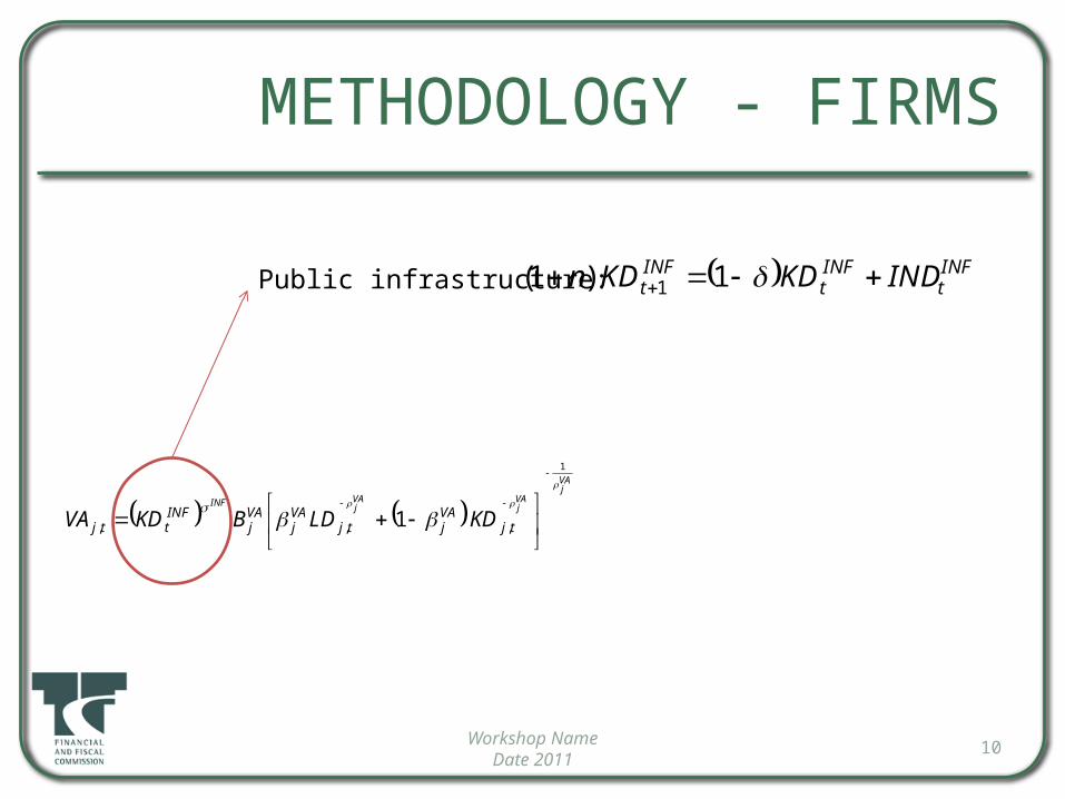
RESULTS-SIMULATION 2
• Although the debt-to-GDP ratio is above that of BAU in the short term, it would be below in the long run because of economic growth
31Workshop Name
Date 2011
20112013
20152017
20192021
20232025
20272029
20312033
20352037
20392041
20432045
20472049
20512053
20552057
20590.98
0.99
1
1.01
1.02
1.03
1.04
BAU SIM2-direct tax SIM2-indirect tax SIM2-Debt

RESULTS-SIMULATION 2
• Different values of elasticity would change the amplitude of the impact on GDP by less than 1%.
32Workshop Name
Date 2011
2011
2012
2013
2014
2015
2016
2017
2018
2019
2020
2021
2022
2023
2024
2025
2026
2027
2028
2029
2030
2031
2032
2033
2034
2035
2036
2037
2038
2039
2040
2041
2042
2043
2044
2045
2046
2047
2048
2049
2050
2051
2052
2053
2054
2055
2056
2057
2058
2059
99.4
99.6
99.8
100
100.2
100.4
100.6
100.8
101
101.2
BAU 0.1-direct tax 0.1-indirect tax0.1-Debt 0.3-direct tax 0.3-indirect tax0.3-Debt 0.6-direct tax 0.6-indirect tax0.6-Debt

RESULTS-SIMULATION 2
• Similar conclusion for the debt-to-GDP ratio
33Workshop Name
Date 2011
2011
2012
2013
2014
2015
2016
2017
2018
2019
2020
2021
2022
2023
2024
2025
2026
2027
2028
2029
2030
2031
2032
2033
2034
2035
2036
2037
2038
2039
2040
2041
2042
2043
2044
2045
2046
2047
2048
2049
2050
2051
2052
2053
2054
2055
2056
2057
2058
2059
0.970000000000001
0.975000000000001
0.980000000000001
0.985000000000001
0.990000000000001
0.995000000000001
1
1.005
BAU 0.1-direct tax 0.1-indirect tax0.1-Debt 0.3-direct tax 0.3-indirect tax0.3-Debt 0.6-direct tax 0.6-indirect tax0.6-Debt

CONCLUSIONS
• Current expenditures:– Increase in current expenditures has little impact on the economy– Including TFP impact would significantly change the results.
(Would a 5-year increase be sufficient to impact TFP?)– Debt financing would require future intervention in order to go
back to the initial debt-to-GDP ratio.
34Workshop Name
Date 2011

CONCLUSIONS
• Investment expenditures:– Short term public investment in infrastructure would affect TFP– Positive impact on macroeconomic impacts, especially in the
medium run– Reduces the debt-to-GDP ratio, regardless of the financing
mechanism (economic growth).
35Workshop Name
Date 2011