Fiscal policy in a monetary union:

Optimal policy and cross-country spillovers

Thomas Bourany∗

Master thesis – Economics and Public Policy

Sciences-Po – École Polytechnique – Ensae

November 2017

Abstract

What are the effects of fiscal policy in a monetary union? This article explores the role of gov-

ernment spending, the optimal policy design and the various spillovers of public spending shocks in an

integrated union. To this purpose, we develop a two-countries model with "large economies", updating

the conclusions at stake in "small open economy" models, and providing a general framework where coun-

tries differ on many aspects – home-bias, agents preferences, price rigidities and labor supply. We show

first that interaction effects and structural heterogeneity matter for optimal policy: the clear separation

between central bank stabilizing the union and fiscal policies stabilizing country-specific shocks will not

hold in this setting. Our second set of results is to identify the main transmission mechanisms of fiscal

policy, with first a trade channel, through relative prices, and second a monetary response from the union

central bank. Our main conclusion is that spillovers of fiscal policy shocks crucially depend on the central

bank mandate and the second channel largely dominates the first in this setting. This framework provides

arguments supporting coordination between union central bank and fiscal authorities in the context of

the European Monetary Union.

∗thomas.bourany@sciencespo.frI would like to thank my supervisor Jean-Baptiste Michau for his patient and encouraging support and his helpfulcomments all throughout this work. I would also like to thank all my professors and past advisors for giving methe will to continue in this field, and my classmates for their advice. All errors are mine.

1

1 Introduction

The recent crisis has revealed that one of the major challenges of European Union is fiscal.

If one hope to complete the EU, in particular in Eurozone, its main currency and monetary

union, one would have to rethink the role of fiscal policy. According to the "Five Presidents’

Report", the Euro Area needs to introduce an advisory European Fiscal Board "coordinating and

complementing national fiscal councils", before implementing a "common stabilisation function"

with budgetary instruments. When monetary policy fails to stabilize large adverse shocks in

situation of liquidity trap, such fiscal framework would strengthen the policy responses, while

leaving idiosyncratic national shocks to the member states.

However, such clear-cut separation between asymmetric vs. aggregate stabilization – per-

formed at country vs. union-level – may fail to address several issues at stake: the European

crisis has shown powerful cross-country transmission channels, due to trade and financial inte-

gration. In particular, fiscal policy may react to shocks originated from neighboring countries or

may itself imply policy spillovers on the rest of the Union.

This papers addresses these two questions: what are the transmission channels of gov-

ernment spending shocks and should fiscal policy be used to stabilize asymmetric shocks in a

monetary union? The contribution is this paper is thus twofold: we first identify the cross-

country spillovers of fiscal policy, and then determine the optimal policy in this monetary union.

To this purpose, I develop a two-countries DSGE model with two large economies: I advocate

that Small-Open-Economy models fail to identify cross-country transmission channels due to the

lack of interaction effects: shock in one country affects the other country’s decisions, which in

turn amplifie the original shock, and so on. Moreover, I provide a general framework where the

two countries differ on many aspects: home-bias, agents preferences, price rigidities, labor sup-

ply, etc. As cross-country effects are not symmetrical anymore, the consequences of an aggregate

shock or central bank policy may affect one country more severely than the other.

With these two characteristics, I provide a more accurate vision of the spillovers of govern-

ment spending, and how interact the two countries’ households, local fiscal authorities and the

union-central bank. I choose to focus on a tractable New-Keynesian model, adding governments

that provide public goods to representative households. This very general environment differs

from the preexisting literature mainly to account for structural heterogeneity and interaction

effects.

2

This paper offers both normative and positive analyses. First, we establish general results

about optimal policies – at the first and second best – and we build upon this analysis to discuss

policy implications for the EMU. The main message is that country structural heterogeneity

complicate the welfare investigation and require a greater cooperation between the different

stabilisation instruments. In particular, both the first-best allocation and the union loss function

display novel "wedges" and "weights" depending on home-bias and labor supply elasticity. Using

this welfare criterion for policy analysis, the optimal policy for central bank and national fiscal

authorities reduces fourfold the welfare loss in case of asymmetric supply shocks. Fiscal policies

can reduce trade imbalances and relative price differential that overload labor markets of one

country. Moreover, we show that optimal policy can be replicated by means of simple monetary

and fiscal policy rules – where central bank follows the standard Taylor principle and government

spendings react to terms-of-trade and output gaps. The presence of structural heterogeneity

provide a rationale for cooperation: to reach the optimum, the central bank should account for

government spending adjustment and conversely.

Second, we turn to more positive implications and identify spillovers of fiscal policy shocks.

The main result is the presence of two transmission channels: public spending in one country

results in domestic inflationary pressures: This policy distorts terms-of-trade, as foreign goods

are relatively cheaper, and private consumption for domestic-good decreases. This first trade

channel appears both in small-open economy and large economy framework. The key insight

when focusing on large-economies is to understand the impact of monetary policy reaction. In

small-open economy, the domestic country, being negligible, has no impact on the union, while

with two large economies, the effects of government purchases affects the union inflation: the

central bank will therefore react to spending shocks, raising interest rate. As a result, this

interest hike affects negatively the foreign country, where consumption decreases, output gap

widens and prices fall. Therefore, the fiscal policy in a country may have a deflationary impact

on its neighbor through central bank reaction. Such transmission channel is at the heart of

our result and undermine common assessments from the small-open economy framework. The

spillovers of fiscal policy of one country for its neighbors show a positive trade effect due to

distorted terms-of-trade and a negative impact of central bank reaction, the second being much

stronger in this setting.

3

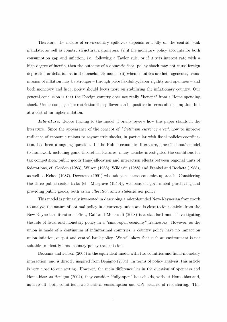
Therefore, the nature of cross-country spillovers depends crucially on the central bank

mandate, as well as country structural parameters: (i) if the monetary policy accounts for both

consumption gap and inflation, i.e. following a Taylor rule, or if it sets interest rate with a

high degree of inertia, then the outcome of a domestic fiscal policy shock may not cause foreign

depression or deflation as in the benchmark model, (ii) when countries are heterogeneous, trans-

mission of inflation may be stronger – through price flexibility, labor rigidity and openness – and

both monetary and fiscal policy should focus more on stabilizing the inflationary country. Our

general conclusion is that the Foreign country does not really "benefit" from a Home spending

shock. Under some specific restriction the spillover can be positive in terms of consumption, but

at a cost of an higher inflation.

Literature : Before turning to the model, I briefly review how this paper stands in the

literature. Since the appearance of the concept of "Optimum currency area", how to improve

resilience of economic unions to asymmetric shocks, in particular with fiscal policies coordina-

tion, has been a ongoing question. In the Public economics literature, since Tiebout’s model

to framework including game-theoretical features, many articles investigated the conditions for

tax competition, public goods (mis-)allocation and interaction effects between regional units of

federations, cf. Gordon (1983), Wilson (1986), Wildasin (1988) and Frankel and Rockett (1988),

as well as Kehoe (1987), Devereux (1991) who adopt a macroeconomics approach. Considering

the three public sector tasks (cf. Musgrave (1959)), we focus on government purchasing and

providing public goods, both as an allocation and a stabilization policy.

This model is primarily interested in describing a microfounded New-Keynesian framework

to analyze the nature of optimal policy in a currency union and is close to four articles from the

New-Keynesian literature. First, Galí and Monacelli (2008) is a standard model investigating

the role of fiscal and monetary policy in a "small-open economy" framework. However, as the

union is made of a continuum of infinitesimal countries, a country policy have no impact on

union inflation, output and central bank policy. We will show that such an environment is not

suitable to identify cross-country policy transmission.

Beetsma and Jensen (2005) is the equivalent model with two countries and fiscal-monetary

interaction, and is directly inspired from Benigno (2004). In terms of policy analysis, this article

is very close to our setting. However, the main difference lies in the question of openness and

Home-bias: as Benigno (2004), they consider "fully-open" households, without Home-bias and,

as a result, both countries have identical consumption and CPI because of risk-sharing. This

4

restriction changes the general result, as trade transmission channel is absent. For this reason,

the gains from stabilization of asymmetric shocks by fiscal policy are likely to be underestimated.

Hence, we differ from this model, and adopt a more general setting.

Nevertheless, they also study country heterogeneity on policy tradeoffs, focusing on nominal

rigidities. They conclude that monetary policy should implement a weighted-average inflation

targeting rule, with more weight on the region with higher degree of price stickiness. We obtain a

similar – but more general – result with weighted average, the weight accounting for supply-side

factors: price stickiness but also labor-supply elasticity and agent preferences. In a different

fashion, Liu and Pappa (2008) emphasize the importance of dissimilarity in trading structures –

tradable/non-tradable sector – for macroeconomic coordination.

This paper also stand in the literature focusing on the effects of government spending and

fiscal multipliers. Christiano, Eichenbaum and Rebelo (2011), Galí, López-Salido and Vallés

(2007) and Farhi and Werning (2012b) emphasize the importance of either non-separable prefer-

ences, presence of credit-constrained households or the absence of monetary reaction – at the ZLB

– to generate high fiscal multipliers: inflationary public spending, in situation of positive wealth

effects of labor supply or liquidity trap, reduces real interest rate and consumption reacts posi-

tively. In a currency union however, these effects are strikingly different, due to terms-of-trade

distortion. When government spending appreciates terms-of-trade, this dampens consumption

and the multiplier can be lower than one. Most of our result are analogous to the analysis of

Farhi and Werning (2012b), but our framework display the interaction effects and implications

from structural heterogeneity, absent from the small-economy model of their article.

Several articles such as Correia, Farhi, Nicolini and Teles (2013), Farhi, Gopinath and

Itskhoki (2014), Farhi and Werning (2012a), also discussed innovative actions for government in-

tervention. Using distortive taxes, government can "mimic" the path on interest rate or exchange

rate, or fiscal-union can provide insurance via contingent transfers to cover against asymmetric

shocks. However, distortive taxation can undermine greatly the positive impact of government

spending, as discussed in Drautzburg and Uhlig (2015). Ferrero (2009) use a framework similar

to Galí and Monacelli (2008) but including distortive taxation and government debt. However,

I choose to focus solely on government spending policy, as taxes are always slower to react for

stabilization motives.

5

Considering the research question and motivation we draw inspiration from the recent

article by Blanchard, Erceg and Lindé (2017). This article also measure the effect of a fiscal ex-

pansion in the "Core" economies of Euro Area to improve economic outcomes of the "Periphery"

using a medium and a large-scale DSGE model, they show that trade channel is at the center

of the mechanism, along with the lack of reaction by central bank – i.e. liquidity trap here. As

they use quantitative models with a large number of features, it can be relevant to describe the

transmission channels with a relatively simple and tractable model.

A last word on the empirical relevance of the two channels of fiscal policy in a currency

union. As described in Beetsma and Giuliodori (2011) a fiscal shock can be followed by a rise

in output and consumption but a reduction in trade-balance. This characterizes the "leakage

effect" we describe, due to terms-of-trade distortions. Carlino and Inman (2013) also study the

spillover of state-deficit policy in United States in terms of employment. This question is also

addressed in Hebous and Zimmermann (2013), who use "Global VAR" to study the spillover of

a fiscal shock in Euro Area, and compare unilateral vs. coordinated fiscal actions and show that

the latter have much larger effect. We can also consider evidences from Poghosyan et al. (2014)

on how fiscal transfers can smooth regional shock in established federation.

The rest of the paper is organized as follow: the next section develop the two-country

DSGE model. In the third section, we step aside to determine the optimal allocation at the

first-best. The efficient allocation is necessary to understand what kind of policy trade-offs the

economy faces in presence of nominal rigidities and how to derive the welfare criterion, as we

shall see in the fourth section and the fifth, where we derive the optimal policy by mean of simple

rule. The sixth and seventh chapters present the policy experiments, the effects of the models

subject to respectively technology shock and fiscal policy shocks. The last develop on the role

for structural heterogeneity, which is the main rationale of this paper for cooperation between

the union central banks and fiscal authorities.

6

2 A two-countries DSGE model

In this model, the currency union is a closed system made of two countries (Home and Foreign) of

identical "unit" size. The "Home" economy is denoted with standard variables, while Foreign is

denoted with stars (*). As presented in introduction, the two countries are not isomorphic, and

that explains why the following formulas might be slightly heavier than in Small-Open Economy

models. Here are the main features of the model:

Households

Each country is made of a representative-household maximizing utility E0∑∞

t=0 βtU(Ct, Gt, Nt)

positive in private (Ct) or public (Gt) consumption and negative in labor supply (Nt).

Consumption Ct (or C∗t ) are subject to Home-bias. As a CES aggregator, it is composed

of domestic (CH,t) or imported (CF,t) goods, with the Home-goods share represented by an index

α. If α < 1/2, this reflects a Home-bias, while α, α*→ 1/2 represents full openness. Note that the

bias may be different for the foreign country (if α < α*, Home is less open).

Goods produced in each country (CJ,t, J = H,F ) are made of a continuum of varieties

(again CES aggregators) and where ε represents elasticity of substitution across varieties.

Household face a budget constraint (j representing Home or Foreign – with ∗):

∫ 1

0CjH,t(i)PH,t(i)di+

∫ 1

0CjF,t(i)PF,t(i)di+ Et{Qt,t+1D

jt+1} ≤ D

jt +W j

t Njt − T

jt

where PH,t & PF,t represent production prices at Home and Abroad, Djt+1 the payoff of the

Household portfolio, Qt,t+1 the stochastic discount factor for one-period ahead nominal payoff,

W jt the nominal wage and T jt the lump-sum tax. Here we suppose that law of one price holds

and PH,t(i) = P ∗H,t(i).

The first-step optimization yields demand-schedules where consumption levels are in-

versely related to prices, and we then define aggregate price indices and CPI (consumer price

index Pt and P ∗t ) are Cobb-Doublas depending on openness α (or α*).

The union economy is a Currency-Union and exchange rate is pegged. Terms-of-trade

variable is key and defined as St =PF,tPH,t

. The Real-Exchange Rate follows: Rt =P ∗tPt

= S(1−α−α*)t

7

Household utility is separable and logarithmic in consumption of private and public goods

and CRRA in labor: U(Ct, Gt, Nt) ≡ (1− Γ) log(Ct) + Γ log(Gt)− N1+ϕt

1+ϕ , where Γ ∈ [0, 1) is the

weight attached to public goods and ϕ the disutility of labor supply by household (i.e. the inverse

of Frisch elasticity). These two parameters are heterogeneous across countries: the "taste" of

household for public good (e.g. Social service, Health or Education) can differ i.e. Γ∗ 6= Γ, as

well as disutility of working (e.g. due to labor supply constraints) i.e. ϕ∗ 6= ϕ.

Deriving a second-step optimization, we obtain the two standards relations describing

Household behavior: Euler equation (LHS) and Consumption-Leisure tradeoff (RHS):

Qt,t+1 = β( PtPt+1

)( CtCt+1

)CtN

ϕt = (1− Γ)

Wt

Pt

In this union, financial markets are complete, i.e. this currency union is perfectly fi-

nancially integrated as there exists a full set of state-contingent Arrow-Debreu securities traded

across countries. The stochastic-discount factor are equalized between Home and Foreign. This

leads to:

Ct+1

Ct=C∗t+1

C∗t

(Rt+1

Rt

)⇒ Ct = ϑ0C

∗t Rt = ϑ0C

∗t S1−α−α*

t

ϑ0 represents NFA position differentials: this parameter introduces a wedge between Home and

Foreign consumption due to heterogeneous preferences. The determination will be discussed

latter, but ϑ0 will intuitively stand for the asymmetry in private/public goods preferences (and

directly, government size) under the ratio : ϑ0 = 1−Γ1−Γ∗ . This value will be consistent with a

null-trade-balance at steady-state between the two countries1.

Government and monetary policy

The currency-union is a monetary-union. There is a single Central-bank and short term

interest-rate it that apply to both Home and Foreign countries.

Governments produce public goods Gt (or G∗t ) in the two countries2. Public goods are

produced from a CES aggregation of intermediary goods bought to firms. The public good output

is entirely consumed by Households, either at Home or Abroad: the Home Household can consume

"Foreign" public goods with a share αG (and "Home" public goods with a share 1− αG). Again,

1This wedge is consistent with a feature developed in Liu and Pappa (2008) introducing such a wedge toaccount for asymmetry in trading structures between the two countries. In their article, ϑ0 is the ratio of tradablesector shares, while ours is the ratio of private sectors

2The optimal level of "government purchase" will be in the center of our normative analysis in the next section

8

Foreign household may consume a different share of Home public goods (αG* 6= αG). Therefore,

government spending Gt can be represented by a Cobb-Douglas function with parameter αG.

Demand schedules for public goods and government price indices are similar to private goods,

but depending on "government openness"3.

Government purchase is financed through lump-sum taxes and government has a bal-

anced budget. Here, we abstract from central features for fiscal multiplier determination (namely

debt issuance and taxes adjustment) and these points might deserve extensions.

Firms and production

A continuum of firms is producing intermediary goods under monopolistic-competition in

each country. The technology is linear in labor Nt, and subject to productivity shocks At. This

TFP (At or A∗t ) follow an AR(1) process with persistence ρa ∈ [0, 1] and white-noisy shocks {εat }.

Aggregation of firms output using CES technology yield the standard Yt = AtNt ∆t, where

∆t is the coefficient of price dispersion.

Marginal cost is defined as real wages Wt/PH,t, accounting for employment subsidy τ and

divided by the marginal productivity. Because production is linear, all firms have the same

marginal cost.MCt = (1− τ)

Wt

PH,t

Nt

Yt= (1− τ)

Wt

Pt

Nt

Yt(St)

α

Here, terms of trade impact positively marginal costs as real wage – relatively to consumer prices

– are appreciated when terms of trade are depreciated, increasing the cost.4.

Prices are subjects to Calvo-Yun rigidities, with a share θ of firms not allowed to reset

their prices. Price stickiness θ is heterogeneous between Home and Abroad (i.e. θ 6= θ∗), and

firms resetting prices face profit-maximization problem. First-order condition yields the optimal

price level as a function of marginal cost and mark-up (M = εε−1), and as a result, under flexible

price we obtainM−1 = MCt ∀t.

Log-linearization of the main relations

We will approximate the main equations of this model around the Steady-State. For each variable

Zt, this log-deviation is denoted zt ≡ lnZt − lnZ = zt − z where Z represent the steady-state

value and zt its log-value.

3This parameter that will be important for transmission of inflation from one country to the other4Note that this formula is similar for the Foreign country, adding stars to the other variables, with τ 6= τ∗

9

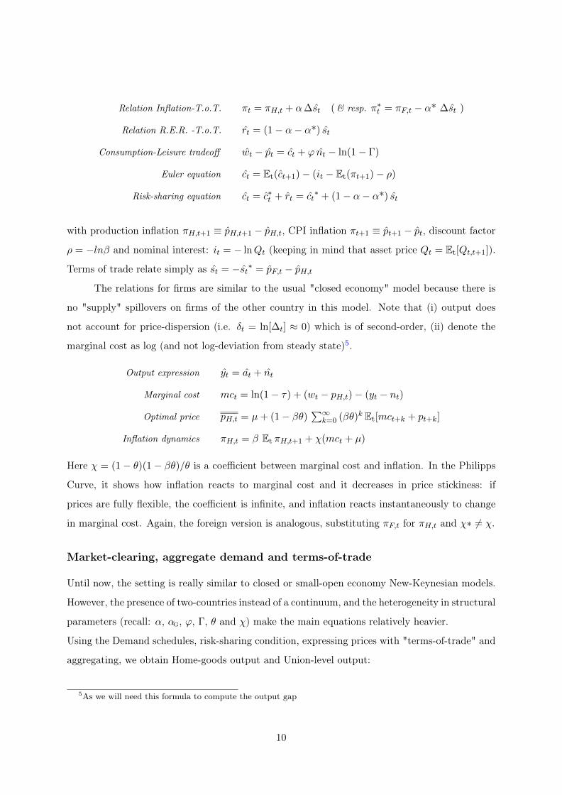
Relation Inflation-T.o.T. πt = πH,t + α∆st (& resp. π∗t = πF,t − α* ∆st )

Relation R.E.R. -T.o.T. rt = (1− α− α*) st

Consumption-Leisure tradeoff wt − pt = ct + ϕ nt − ln(1− Γ)

Euler equation ct = Et(ct+1)− (it − Et(πt+1)− ρ)

Risk-sharing equation ct = c∗t + rt = ct∗ + (1− α− α*) st

with production inflation πH,t+1 ≡ pH,t+1 − pH,t, CPI inflation πt+1 ≡ pt+1 − pt, discount factor

ρ = −lnβ and nominal interest: it = − lnQt (keeping in mind that asset price Qt = Et[Qt,t+1]).

Terms of trade relate simply as st = −st∗ = pF,t − pH,t

The relations for firms are similar to the usual "closed economy" model because there is

no "supply" spillovers on firms of the other country in this model. Note that (i) output does

not account for price-dispersion (i.e. δt = ln[∆t] ≈ 0) which is of second-order, (ii) denote the

marginal cost as log (and not log-deviation from steady state)5.

Output expression yt = at + nt

Marginal cost mct = ln(1− τ) + (wt − pH,t)− (yt − nt)

Optimal price pH,t = µ+ (1− βθ)∑∞

k=0 (βθ)k Et[mct+k + pt+k]

Inflation dynamics πH,t = β Et πH,t+1 + χ(mct + µ)

Here χ = (1− θ)(1− βθ)/θ is a coefficient between marginal cost and inflation. In the Philipps

Curve, it shows how inflation reacts to marginal cost and it decreases in price stickiness: if

prices are fully flexible, the coefficient is infinite, and inflation reacts instantaneously to change

in marginal cost. Again, the foreign version is analogous, substituting πF,t for πH,t and χ∗ 6= χ.

Market-clearing, aggregate demand and terms-of-trade

Until now, the setting is really similar to closed or small-open economy New-Keynesian models.

However, the presence of two-countries instead of a continuum, and the heterogeneity in structural

parameters (recall: α, αG, ϕ, Γ, θ and χ) make the main equations relatively heavier.

Using the Demand schedules, risk-sharing condition, expressing prices with "terms-of-trade" and

aggregating, we obtain Home-goods output and Union-level output:

5As we will need this formula to compute the output gap

10

YH,t =[(1− α) + ϑ−1

0 α∗]Sαt Ct + (1− αG)SαG

t Gt + αG*S1−αG*t G∗t

YW,t ≡ YH,t + YF,t = SWH,C

t Ct + SWF,C

t C∗t + SWH,G

t Gt + SWF,G

t G∗t

where the variables SWH,C

t , SWF,C

t , SWH,G

t and SWF,G

t are functions6 of terms-of-trade and shift

aggregate demand due to price differentials. For example, for Home-consumption, this wedge

decreases exponentially (with power 1 − α) when terms of trade are appreciated (i.e. St < 1)

and increases logarithmically (power α) when depreciated (i.e. St > 1). Intuitively, this explains

why, when Home-goods are relatively cheaper (St > 1), the Home-household consume more of its

own goods, increasing demand for Home-production. This effect comes directly from Home-bias

in consumption is undermined if country are more open. Therefore, with balanced terms-of-trade

(St = 1), SW·,·t collapse to 1 and YW,t = Ct + C∗t +Gt +G∗t .

When log-linearized around a symmetric steady-state, we use some specific notations.

To avoid multiplying the parameters, the steady-state demand aggregates can be expressed as

share of world output (Yw = C+C∗+G+G∗) and are denoted γC , γC*, γG and γG* respectively for

C,C∗, G,G∗ over Yw. However, we also make the assumption (A1) that the two countries have

the same size (unity). As a result, steady-state demand should not be higher that country size

and we will suppose symmetry in steady-state output (which is not as restrictive as homogeneity)

and we have Y = Y ∗ = 1/2Yw. These two points will slightly constrain parameters values but

the formula obtained is reduced to:

1/2 yH,t = (1− α) γC ct + α∗ γC* c

∗t + (1− αG) γG gt + αG* γG* g

∗t + ω st

where ω is a parameter7 increasing in openness and zero in complete autarky. Once again, this

represents the distortion implied by terms of trade differences: if terms of trade are depreciated,

home goods are relatively cheaper for all the agents, increasing demand for Home-goods by a

factor ω8. Note that ω = ω∗ this effect is symmetric on Home and Foreign.

We know from the previous section that "Home goods" are consumed by the "World-

household" with a share9 {(1−α) γC +α∗ γC*}. As we will need it in a latter section, we introduce

a new notation with the parameter ΞH ≡ (1− α) γC +α∗ γC* and ΞF ≡ (1− α∗) γ

C* +αγC .

6For example for Home consumption: SWH,Ct ≡ (1− α)Sαt + αS1−α

t , and other functions are similar.7This parameter is defined as ω ≡ (1− α)αγC +(1− α∗)α∗ γ

C* +(1− αG)αG γG +(1− αG*)αG* γG*8For example, if the Home-household is completely open, the terms of trade appreciation (st negative) will

dampen the home-good demand, both in quantity (large share of foreign goods consumed) and price (demandschedule strongly affected by relative prices)

9A share (1− α) γC domestically and α∗ γC* imported by the Foreign household.

11

Using this new parameter, we make another assumption (A2). Because of the risk-

sharing condition, the two households – in Home and Foreign – should consume the same amount,

modulo a term-of-trade difference. Therefore, the share of home-good ΞH in the world-household

basket should be equivalent to the share of Home-consumption i.e. γC = C/Y w as described

above (and similarly for the Foreign country: ΞF = γC*). Manipulating the terms, we obtain

necessary the following restriction α∗ γC* = αγC . The intuition behind this constraint is an equal

size private-goods trade between the two countries at steady-state. The two countries should

consume the same amount of imported consumption goods at steady-state. If one country run

a trade surplus for some time, he will save more, and consume more in the future (Home and

Foreign) goods. In absence of other shocks, this adjustment will bring trade back to a "balanced"

equilibrium. This second condition on parameters (implied by the risk-sharing assumption), is

relatively stronger, but it is still valid to preserve heterogeneity.

Euler equations and Philipps Curve

We will recall and extend the main equations driving demand and supply in such a New-Keynesian

model. First, the dynamic (forward-looking) Euler equations at Home10 and at the Union-

level11 rewrites:ct = Et(ct+1)− (it − Et(πH,t+1)− ρ) + α Et(∆st+1) (1)

cw,t = Et cw,t+1 − {(γC + γC*)[it − ρ]− (ΞH Et πH,t+1 + ΞF Et πF,t+1)}

Aside the usual determinants of consumption (real interest rate, future consumption), the Home-

consumption is also driven by terms-of-trade depending on openness α. Furthermore, the union-

level equation, which is a key relation for Union-central-bank mandate shows the standard Euler

equation, showing union-level inflation with weights ΞH and ΞF (i.e. share in the union con-

sumption bundle).

Second, we turn to the supply-side and Philipps-Curve. Using descriptions of output,

technology and labor-consumption trade-off, we obtain the formula determining marginal cost

for producing Home-goods12:

mct = ln(1− τ

1− Γ

)+[1 + 2ΞHϕ

]ct + 2ϕ

[(1− αG) γG gt + αG* γG* g

∗t

]+[

α+ 2ϕ(ω − α∗ γC*(1− α− α∗))

]st − (1 + ϕ)at

10And similarly in the Foreign country, using Foreign parameters and an opposite sign for terms-of-trade11Aggregating simply with: cw,t ≡ γC ct + γ

C* c∗t

12Again, this formula hold symmetrically for the foreign country, changing parameter values, and sign for st

12

In this relation, marginal cost is function of real wages, as households request higher wages when

they can consume more or work supplementary hours. As a result, aggregate demand has a direct

effect on marginal costs: higher consumption at Home or Abroad, higher government spending

or terms-of-trade depreciation, through a rise of export, will all imply a higher work effort and

disutility of labor (by a factor ϕ). Another indirect effect of terms-of-trade depreciation appears

through the "relative price" of real wage, especially in "open" economy (high α). Concretely,

wages are chosen by workers on account of CPI level, increasing in terms-of-trade. Therefore,

the more open the country and the more depreciated the relative prices, the higher the requested

wages and costs for firms, compared to producer level PH,t. Finally, productivity and employment

subsidy both reduce marginal costs as in the usual setting.

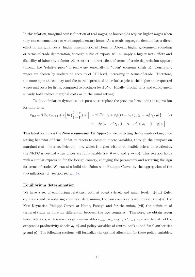
To obtain inflation dynamics, it is possible to replace the previous formula in the expression

for inflations:

πH,t = β Et πH,t+1 + χ[

ln(1− τ

1− Γ

)+[1 + 2ΞHϕ

]ct + 2ϕ

{(1− αG) γG gt + αG* γG* g

∗t

}(2)

+[α+ 2ϕ(ω − α∗ γ

C*(1− α− α∗))]st − (1 + ϕ)at

]This latest formula is theNew Keynesian Philipps-Curve, reflecting the forward-looking price

setting behavior of firms. Inflation reacts to common macro variables, through their impact on

marginal cost – by a coefficient χ – i.e. which is higher with more flexible prices. In particular,

the NKPC is vertical when prices are fully-flexible (i.e. θ → 0 and χ→∞). This relation holds

with a similar expression for the foreign country, changing the parameters and reverting the sign

for terms-of-trade. We can also build the Union-wide Philipps Curve, by the aggregation of the

two inflations (cf. section section 4).

Equilibrium determination

We have a set of equilibrium relations, both at country-level, and union level: (i)-(iii) Euler

equations and risk-sharing condition determining the two countries consumption, (iv)-(vi) the

New Keynesian Philipps Curves at Home, Foreign and for the union, (vii) the definition of

terms-of-trade as inflation differential between the two countries. Therefore, we obtain seven

linear relations, with seven endogenous variables πw,t, πH,t, πF,t, ct, c∗t , cw,t, st given the path of the

exogenous productivity shocks at, a∗t and policy variables of central bank it and fiscal authorities

gt and g∗t . The following sections will formalize the optimal allocation for these policy variables.

13

3 Efficiency and optimal policy

In this section, I follow closely the normative analysis made in Galí and Monacelli (2008). The

aim is to determine the socially-optimal allocation of resources in a no-distortion-economy. We

first analyze the decision of a Social Planner weighting the two countries equally – what we call

a cooperating optimum – and then the decision of two Social Planners, one for each country

– what we call a Nash-bargaining allocation. Third, we show how the cooperating equilibrium

can be decentralized in a flexible-price economy. This cooperating optimum will constitute the

benchmark for policy analysis in presence of nominal rigidities.

Social-planner allocation – cooperating optimum

The cooperating optimal allocation is solving the social planner’s problem. The union’s planner

seeks to maximize the weighted sum of Household utility ωHUH(Ct, Nt, Gt) +ωFUF (C∗t , N∗t , G

∗t )

subject to both resource constraints of the two countries, YJ,t = CJ,t + C∗J,t + GJ,t + G∗J,t for

J = H,F and technological constraint: YJ,t = AJt NJt

Drawing the constrained optimization problem, we derive optimality conditions as the

allocation equalizing the marginal disutility of producing a good with the marginal utility of

consuming the good by the four agents (as public or private good, and at Home or Foreign).

This implies: −∂UW∂YH

= ∂UW∂CH

= ∂UW∂C∗

H= ∂UW

∂GH= ∂UW

∂G∗H

and similarly for the foreign good. We obtain

eight conditions, along with the constraints, and we obtain uniquely the allocation:

CH,t = ωH (1− Γ)(1− α)Atη− ϕ

1+ϕ C∗F,t = ωF (1− Γ∗)(1− α∗)A∗t η∗− ϕ∗

1+ϕ∗

C∗H,t = ωF (1− Γ∗)α∗At η− ϕ

1+ϕ CF,t = ωH (1− Γ)αA∗t η∗− ϕ∗

1+ϕ∗

GH,t = ωH Γ(1− αG)At η− ϕ

1+ϕ G∗F,t = ωF Γ∗(1− αG*)A∗t η∗− ϕ∗

1+ϕ∗

G∗H,t = ωF Γ∗ αG* At η− ϕ

1+ϕ GF,t = ωH ΓαG A∗t η∗

− ϕ∗1+ϕ∗

Nt = η1

1+ϕ η =ωH (1− Γ)(1− α) + ωF (1− Γ∗)α∗ + ωH Γ(1− αG) + ωF Γ∗ αG*

N∗t = η∗ 1

1+ϕ η∗ =ωF (1− Γ∗)(1− α∗) + ωH (1− Γ)α + ωF Γ∗(1− αG*) + ωH ΓαG

We define a new parameter η (and resp. η∗) as "preferences" for Home (resp. Foreign)

goods. The important point here is that labor supply is only function of structural parameters

(this new η and labor disutility ϕ) and is consequently a function of the "tastes" of the four

agents (Home/Foreign, Household/Government).

14

As a result, the optimal allocation of consumption in each country relies on the pref-

erences of both countries. For example, Home consumption of Home goods CH,t depends on

Foreign country tastes α* and αG* (by household or government) through Nt and η. If these

preferences are "high", for instance due to "cultural" reasons, labor supply adjusts to satisfy

both Households, and in particular as exports to Foreign. Because of increasing marginal labor

disutility, this will, in some ways, "crowd-out" Home-consumption. Such phenomenon would not

appear without heterogeneous preferences (i.e. η 6= η∗) as the import/export motives will cancel

out due to symmetry. Furthermore, such "crowding-out effect" of consumption is strengthened

with an inelastic labor supply (and a small ϕ).

If we assume "perfect" coordination, with a social-planner weighting equally the two coun-

tries (ωH = ωF = 1), we could contrast our result with Galí and Monacelli (2008). As in their

framework, the diverse aggregates are determined by productivity (At or A∗t ). However, in our

general setting, the optimal level of output, and by extension consumption, public good provision

and terms-of-trade, relies heavily on "preferences" η and labor rigidity ϕ.

The terms-of-trade term St is worth commenting: in this cooperating optimum, if the tastes

differ between Home and Foreign (η 6= η∗), the ratio displays St a long-run price differential

between the two countries, even in absence of productivity differential. This permanent "un-

balanced" terms-of-trade arise in a cooperating equilibrium especially because agents interiorize

both Home and Foreign resource and technological constraints.

To end this section, we need to know if this cooperating allocation is consistent with the

hypothesis of "union-risk-sharing", as discussed in point 9 of the previous section. Recall that

we obtained Ct = ϑ0C∗t S1−α−α*

t . In this case, the value of the "risk-sharing-wedge" ϑ0 should

be consistent with both a long-run terms-of-trade level and efficient allocation.

This yields a wedge of the form: ϑ0 = 1−Γ1−Γ∗ , weighting relative preferences for private goods

between the two countries (essentially because risk-sharing happens only between Households,

but not governments). Therefore, if Γ > Γ∗, the Home-household have higher preference for

public goods, and ϑ0 < 1 the private consumption will always be higher in the foreign country

than at Home, consistent with intuitions as well as structural parameter heterogeneity.

15

Social-planner allocation – Nash-bargaining allocations

We now consider an allocation where the two countries do not coordinate. Formally, this implies

the existence of two social planners, each of them maximizing the utility of the Household in "its"

country, taking into account its resource and technological constraints, and the one of the world

economy. The main result of this section is that there exists an infinite number of allocations

that are optimal from this point of view. The main point to remember is that, in this setting,

the demand schedule for Home and Foreign goods may not interiorize the resource/technology

constraints of both Home and Foreign countries. As a result, this may cause misallocation of

public goods – relatively to the cooperating case – because of productivity differentials.

Decentralization and flexible-price equilibrium

We want to know how the union can reach (cooperating-)optimality in a decentralized equilib-

rium. In an equilibrium under flexible price, i.e. absent nominal rigidities (and denoted with

upper bar), monopolistic competition is the only remaining distortion. For the production to

reach optimum level, marginal cost should equal firm’s mark-up, i.e.:

M−1 =ε− 1

ε= MCt = (1− τ)

Wt

Pt(St)

α Nt

YH,t

Replacing all the variables known and rearranging, we now suppose that (i) employment

subsidy counterbalances monopolistic competition by setting τ = 1ε and (ii) governments provide

the optimal level of public good, as described above. As a result, we obtain:

η = (1− Γ)(1− α) + (1− Γ∗)α* +Γ(1− αG) + Γ∗ αG*

which is exactly the definition of the term η we stated above. Note that, performing exactly

symmetrical computation for the Foreign country, we obtain an analogous result.

Therefore, decentralized equilibrium can reach optimal allocation. What do we learn then

on the link between preferences η and firms’ marginal costs? First, decentralization is optimal

only when both governments purchase the right amount of public goods and do not "crowd out"

private consumption by "overloading" the two countries’ labor supply. As we detailed above,

public goods provision must account for preferences η and labor disutility ϕ. In such situation,

Households set appropriately their labor supply and marginal cost naturally equals firms mark-

up. Under the two conditions concerning employment subsidy and optimal allocation of public

goods, the flexible-price equilibrium reaches optimality, as shown in Galí and Monacelli (2008).

16

Before returning to the log-linearized version of our model, we find more convenient to make

another assumption (A3). To simplify the result, we make the hypothesis that η = η∗ = 1.

Without this assumption, structural heterogeneity can lead to persistent differences in output,

labor supply, consumptions and terms-of-trade, implying a persistent increase in the market

share of one country. This is inconsistent with (A1) the assumption of equal size we made in

the previous section and to the idea of log-linearization around a symmetric steady-state (where

St = 1). Therefore, we will rule out this case, and set η = η∗ = 1. Rearranging the terms, we

obtain a new constraint on the structural parameters for preferences:

(α∗ − α) + Γ(α− αG) = Γ∗(α*−αG*)

This equation makes the preferences between the two countries closer, i.e. more homogenous.

Said differently, Home and Foreign Households should not have "too different" tastes in order to

impose unitary labor supply and equal size in each country.

What intuition lies behind this assumption? If asymmetry exists in one parameter, for

example, if private consumption home-bias is much stronger at Home than in Foreign (α < α∗),

it should be offset by other heterogeneities: either Foreign household should have high preferences

for public goods and higher Home-bias in public goods, or Home Household have lower preferences

for Public goods. Without such condition, then either Households will not be satisfied with the

binding resources constraint – because of the unitary labor supply – or the optimal allocation

exceed the limited capacity of one country. As a consequence, this condition will impose that

trade-balance is null at steady-state. For example, a trade surplus of private consumption goods

should be balanced by a trade deficit of public consumption.

This constraint is automatically satisfied in two common situations: (i) the two households

have the same home-bias (α = α∗) and government buys only domestic goods (αG = αG* = 0) –

case met almost-everywhere in the open-economy literature – or (ii) the two households have the

same home-bias (α = α∗), the same preferences for public goods (Γ = Γ∗), and each government

have the same Home-bias (αG = αG*). We argue here that we can still preserve heterogeneity

in preferences and keep such constraint satisfied, in order to analyze how heterogeneity affects

transmission of fiscal shocks, when the two policies have diverging optimal allocation paths.

With this simplification, it is easy to rewrite optimal allocation, which is now much closer

to the one described in Galí and Monacelli (2008)

17

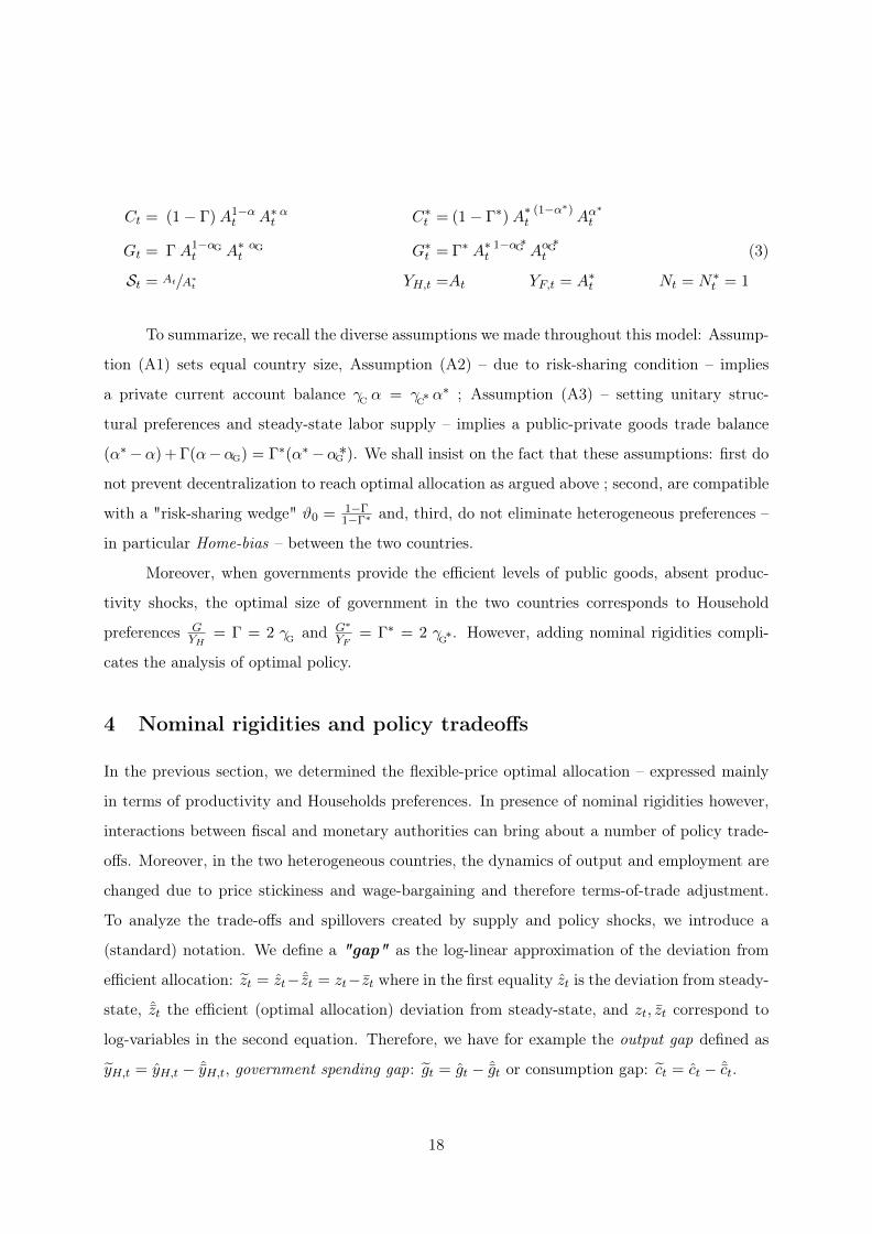
Ct = (1− Γ)A1−αt A∗ αt C∗t = (1− Γ∗)A

∗ (1−α∗)t Aα

∗t

Gt = ΓA1−αGt A∗ αG

t G∗t = Γ∗ A∗ 1−αG*t AαG*

t (3)

St = At/A∗t YH,t =At YF,t = A∗t Nt = N∗t = 1

To summarize, we recall the diverse assumptions we made throughout this model: Assump-

tion (A1) sets equal country size, Assumption (A2) – due to risk-sharing condition – implies

a private current account balance γC α = γC* α

∗ ; Assumption (A3) – setting unitary struc-

tural preferences and steady-state labor supply – implies a public-private goods trade balance

(α∗−α) + Γ(α−αG) = Γ∗(α∗−αG*). We shall insist on the fact that these assumptions: first do

not prevent decentralization to reach optimal allocation as argued above ; second, are compatible

with a "risk-sharing wedge" ϑ0 = 1−Γ1−Γ∗ and, third, do not eliminate heterogeneous preferences –

in particular Home-bias – between the two countries.

Moreover, when governments provide the efficient levels of public goods, absent produc-

tivity shocks, the optimal size of government in the two countries corresponds to Household

preferences GYH

= Γ = 2 γG and G∗

YF= Γ∗ = 2 γ

G*. However, adding nominal rigidities compli-

cates the analysis of optimal policy.

4 Nominal rigidities and policy tradeoffs

In the previous section, we determined the flexible-price optimal allocation – expressed mainly

in terms of productivity and Households preferences. In presence of nominal rigidities however,

interactions between fiscal and monetary authorities can bring about a number of policy trade-

offs. Moreover, in the two heterogeneous countries, the dynamics of output and employment are

changed due to price stickiness and wage-bargaining and therefore terms-of-trade adjustment.

To analyze the trade-offs and spillovers created by supply and policy shocks, we introduce a

(standard) notation. We define a "gap" as the log-linear approximation of the deviation from

efficient allocation: zt = zt− ˆzt = zt−zt where in the first equality zt is the deviation from steady-

state, ˆzt the efficient (optimal allocation) deviation from steady-state, and zt, zt correspond to

log-variables in the second equation. Therefore, we have for example the output gap defined as

yH,t = yH,t − ˆyH,t, government spending gap: gt = gt − ˆgt or consumption gap: ct = ct − ˆct.

18

Policy trade-offs at country level

We can now express the equilibrium relations to underline the policy trade-offs each economy

faces under sticky prices. First, we start with inflation dynamics. Considering firms’ marginal

cost, we know that it equals firm’s mark-up in flexible-price equilibria. Subtracting the efficient

level from the previous formula (mct = mct−mct = mct+µ) and thanks to the relation between

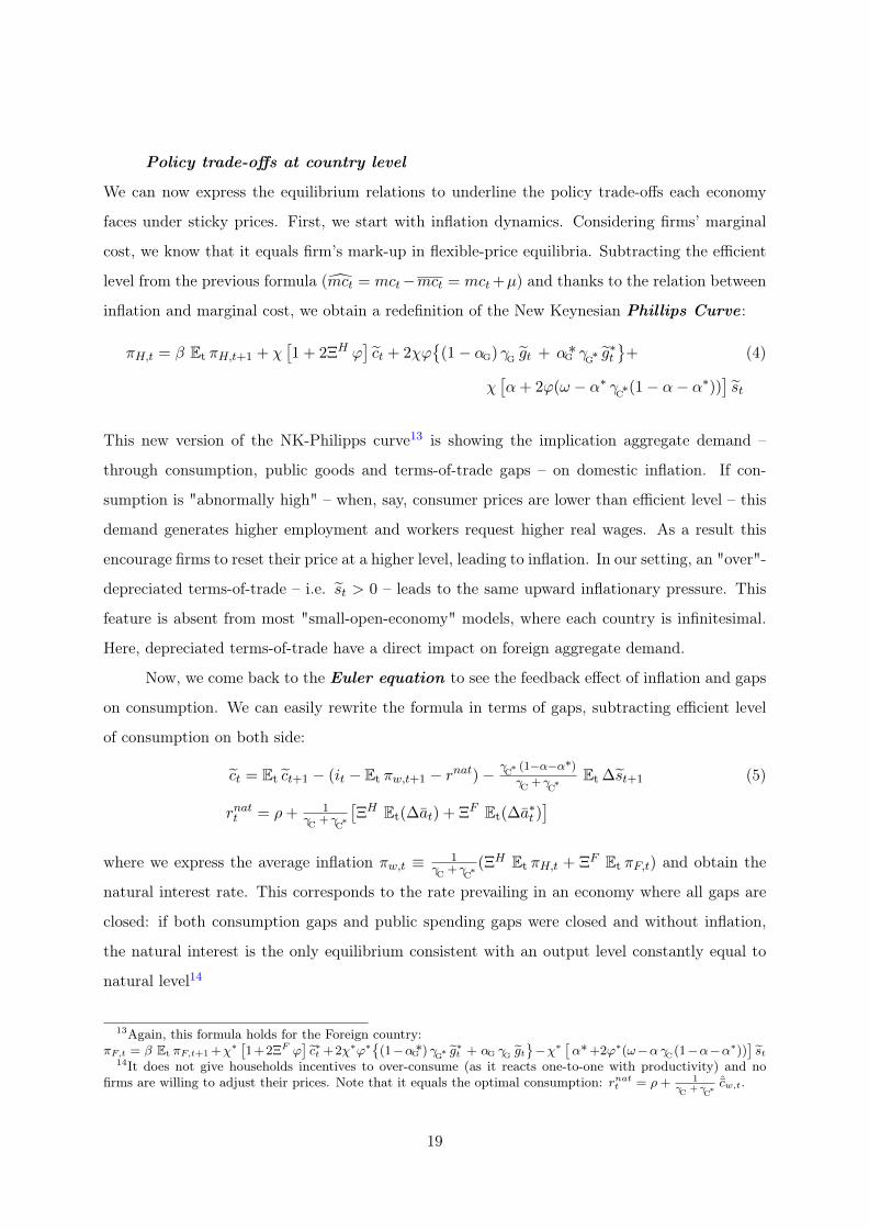
inflation and marginal cost, we obtain a redefinition of the New Keynesian Phillips Curve :

πH,t = β Et πH,t+1 + χ[1 + 2ΞH ϕ

]ct + 2χϕ

{(1− αG) γG gt + αG* γG* g

∗t

}+ (4)

χ[α+ 2ϕ(ω − α∗ γ

C*(1− α− α∗))]st

This new version of the NK-Philipps curve13 is showing the implication aggregate demand –

through consumption, public goods and terms-of-trade gaps – on domestic inflation. If con-

sumption is "abnormally high" – when, say, consumer prices are lower than efficient level – this

demand generates higher employment and workers request higher real wages. As a result this

encourage firms to reset their price at a higher level, leading to inflation. In our setting, an "over"-

depreciated terms-of-trade – i.e. st > 0 – leads to the same upward inflationary pressure. This

feature is absent from most "small-open-economy" models, where each country is infinitesimal.

Here, depreciated terms-of-trade have a direct impact on foreign aggregate demand.

Now, we come back to the Euler equation to see the feedback effect of inflation and gaps

on consumption. We can easily rewrite the formula in terms of gaps, subtracting efficient level

of consumption on both side:

ct = Et ct+1 − (it − Et πw,t+1 − rnat)−γC* (1−α−α*)

γC

+ γC*

Et ∆st+1 (5)

rnatt = ρ+ 1γC

+ γC*

[ΞH Et(∆at) + ΞF Et(∆a

∗t )]

where we express the average inflation πw,t ≡ 1γC

+ γC*

(ΞH Et πH,t + ΞF Et πF,t) and obtain the

natural interest rate. This corresponds to the rate prevailing in an economy where all gaps are

closed: if both consumption gaps and public spending gaps were closed and without inflation,

the natural interest is the only equilibrium consistent with an output level constantly equal to

natural level14

13Again, this formula holds for the Foreign country:πF,t = β Et πF,t+1 +χ∗ [1+2ΞF ϕ

]c∗t +2χ∗ϕ∗{(1−αG*) γ

G* g∗t + αG γG gt

}−χ∗ [α* +2ϕ∗(ω−αγC(1−α−α∗))

]st

14It does not give households incentives to over-consume (as it reacts one-to-one with productivity) and nofirms are willing to adjust their prices. Note that it equals the optimal consumption: rnatt = ρ+ 1

γC

+ γC*

ˆcw,t.

19

Policy trade-offs at union-level

We now turn to Union-level trade offs, especially relevant for union-wide monetary authorities.

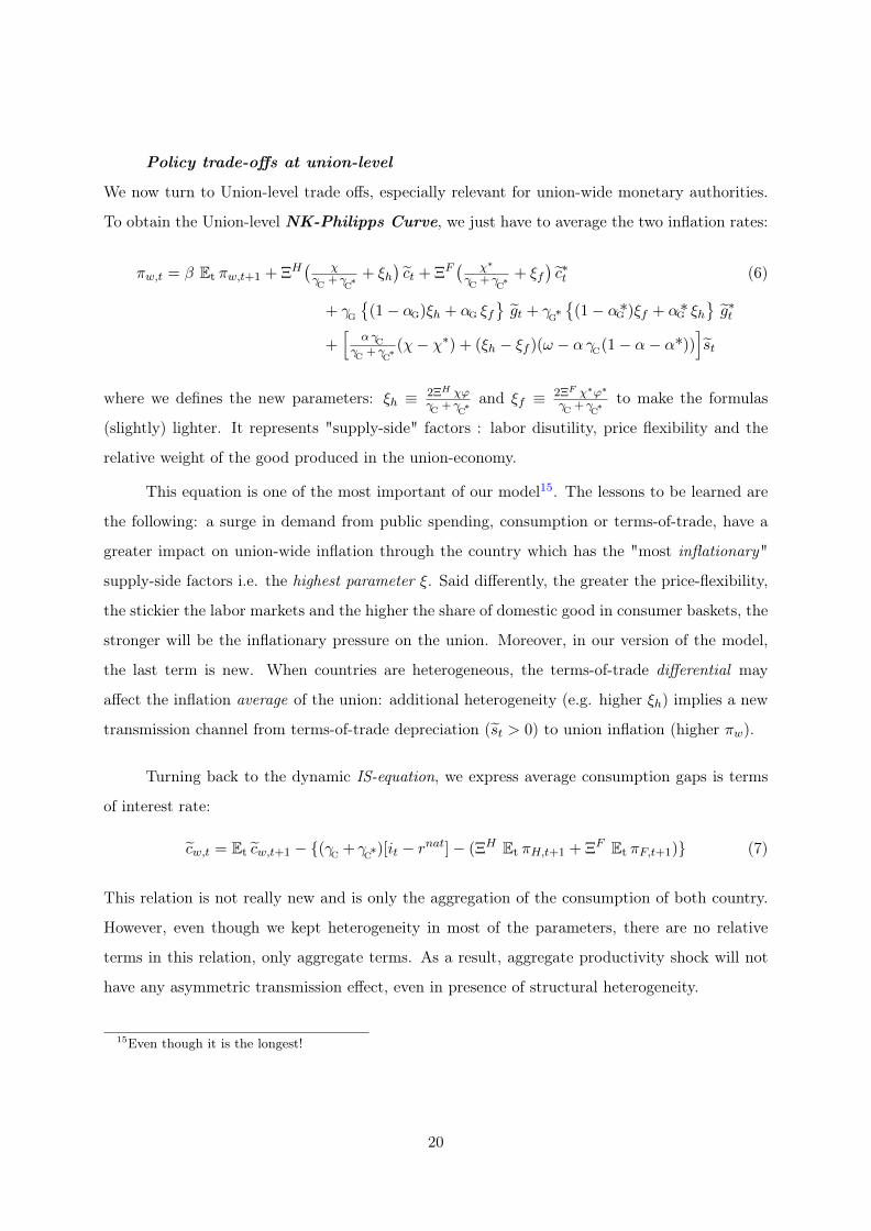
To obtain the Union-level NK-Philipps Curve, we just have to average the two inflation rates:

πw,t = β Et πw,t+1 + ΞH( χγC

+ γC*

+ ξh)ct + ΞF

( χ∗

γC

+ γC*

+ ξf)c∗t (6)

+ γG{

(1− αG)ξh + αG ξf}gt + γ

G*

{(1− αG*)ξf + αG* ξh

}g∗t

+[

αγC

γC

+ γC*

(χ− χ∗) + (ξh − ξf )(ω − αγC(1− α− α*))]st

where we defines the new parameters: ξh ≡ 2ΞH χϕγC

+ γC*

and ξf ≡ 2ΞF χ∗ϕ∗

γC

+ γC*

to make the formulas

(slightly) lighter. It represents "supply-side" factors : labor disutility, price flexibility and the

relative weight of the good produced in the union-economy.

This equation is one of the most important of our model15. The lessons to be learned are

the following: a surge in demand from public spending, consumption or terms-of-trade, have a

greater impact on union-wide inflation through the country which has the "most inflationary"

supply-side factors i.e. the highest parameter ξ. Said differently, the greater the price-flexibility,

the stickier the labor markets and the higher the share of domestic good in consumer baskets, the

stronger will be the inflationary pressure on the union. Moreover, in our version of the model,

the last term is new. When countries are heterogeneous, the terms-of-trade differential may

affect the inflation average of the union: additional heterogeneity (e.g. higher ξh) implies a new

transmission channel from terms-of-trade depreciation (st > 0) to union inflation (higher πw).

Turning back to the dynamic IS-equation, we express average consumption gaps is terms

of interest rate:

cw,t = Et cw,t+1 − {(γC + γC*)[it − rnat]− (ΞH Et πH,t+1 + ΞF Et πF,t+1)} (7)

This relation is not really new and is only the aggregation of the consumption of both country.

However, even though we kept heterogeneity in most of the parameters, there are no relative

terms in this relation, only aggregate terms. As a result, aggregate productivity shock will not

have any asymmetric transmission effect, even in presence of structural heterogeneity.

15Even though it is the longest!

20

In conclusion, it has to be highlighted that government spending can only play a role

through inflation. Consumption/saving decisions are not related to government policies – as

there is no distortive taxes in this setting. However, as shown in the Philipps Curve, government

purchases imposes an extra demand, boosting employment, wage bargaining and raising marginal

costs and inflation. In a second step, this inflation have an influence on consumption and terms-

of-trade, initiating differential between the two countries with the presence of heterogeneity.

In contrast, Central Bank can have a direct impact on consumption of agents, by manip-

ulating the union interest rate. Households interiorize the monetary reaction: they expect the

monetary policy to be more or less aggressive vis-a-vis inflation. As a result, they are influenced

in their consumption, even though interest rate does not change! This effect will be at the center

of policy spillovers, i.e. the responses of Foreign variables after shocks to Home variables. This

analysis will be the topic of the following section.

5 Optimal fiscal and monetary policy with nominal rigidities

In this section and the next, we derive and compute the optimal policy, i.e. the monetary-fiscal

policy mix that would maximize the Union household welfare. For policy evaluation, we derive

a welfare criterion, i.e. the second-order Taylor approximation of Household utility function

in each country. We then consider Utilitarian welfare function aggregating equally the two

utilities. However, if the welfare function provides some insights, the full characterization of the

optimal policy under commitment is relatively heavy16 and provides almost no relevant economic

intuitions. Therefore, we choose not the expose it here. Instead, we choose to expose how fiscal

and monetary policy can replicate the optimal policy using simple monetary and fiscal rules.

Welfare loss function

The second order approximation of the utility function of both Households yields the following

synthetic expression, with t.i.p. the terms independent of policy (namely productivity shocks)

and O(‖ξ‖3) terms of third or higher order:

16Seven additional (and really long...) equations, including five non-instructive Lagrange multipliers, for eachequilibrium relations of the model

21

W =

∞∑t=0

βt Et(Lwt ) + t.i.p. + O(‖ξ‖3) (8)

Lwt = ε2χ π

2H,t + ε

2χ∗ π2F,t + γC c 2

t + γC* c

∗ 2t + γG g 2

t + γG* g

∗ 2t + ω s 2

t

(cw,polt )2 + (gw,polt )2 + (sw,polt )2 + cw,polt · gw,polt + cw,polt · sw,polt + gw,polt · sw,polt

where the terms denoted by "w,pol" are defined as weighted average of variables at Home and inthe Foreign country. They are represented using vectors (and quadratic terms are thus productof two vectors) and account for the countries heterogeneity, in particular agents tastes and labordisutility. As a result, we defined "w,pol", the "policy average" as follow:

cw,polt ≡Ml

cw,Ht

cw,Ft

gw,polt ≡Ml

gw,Ht

gw,Ft

sw,polt ≡Ml

2ω st

−2ω st

where cw,H/Ft (resp. g

w,H/Ft and ± 2ω st) are the gaps in union-consumption (resp. public

spending and terms-of-trade) that affects supply of Home/Foreign goods. Therefore, differences

in labor supply elasticity are included in Ml. More formally:

Ml ≡

√2ϕ 0

0√

2ϕ∗

cw,Ht ≡ γC (1− α) ct + γC* α* c∗t

cw,Ft ≡ γC*(1− α*) c∗t + γC α ct

gw,Ht ≡ γC (1− αG) gt + γG* αG* g

∗t

gw,Ft ≡ γC*(1− αG*) g∗t + γG αG gt

Welfare loss features quadratic terms and cross products, in inflation (i), in consumption and

public spending (ii), in weighted average of consumption and government spending (iii), and in

terms-of-trade (iv). We use a notation using matrices, slightly more convenient and synthetic17.

Inflations (i) appears in the loss function, as usual in the New-Keynesian framework be-

cause price dispersion distorts households consumption. The factor for inflation is increasing in

substitutability across goods (ε) and in price rigidity (i.e. decreasing in χ).

All the remaining terms show aggregate demand effects: "gaps" increase welfare loss

through labor demand, implying workers’ disutility. (ii) The first terms in consumption, govern-

ment spending and terms-of-trade gaps affect labor supply of both countries equally, according

to their weights in the economy (c.f. first line terms, with factors γC , ..., ω). These terms can be

gathered in simple "output gaps", rather standard in the literature.

However, another set of terms (iii), that we define as "policy-weighted average" (e.g. cw,polt )

17In particular, with vectors, it is easier to express cross-products in terms of union-level variable. However,we misused the notation and we should more rigorously note that quadratic terms cw,polt are in fact product ofmatrices, i.e. (cw,polt )2 = (cw,polt )T (cw,polt )

22

shows more intricate linkages between demand of the two countries: they depends on demand

effects direction toward Home or Foreign (i.e. cw,Ht vs. cw,Ft ), private sector size or government

size (i.e. γC , γG), openness (i.e. α, αG), and labor supply elasticity (i.e. ϕ, ϕ∗), included in

Ml. These variables are quadratic in consumption, in government spending gaps (the first two

terms denoted by "w,pol") or feature cross-product interactions between the two sets of aggregate

demand (the fourth term of the second line). In one way or another, these terms appear in most

of the welfare objectives highlighted in the open-economy literature.

However – and this is our last point – terms-of-trade gap (iv) should deserve a closer look.

In small-open-economy models, terms-of-trade gap does not appear in the welfare objective of the

Union due to the infinitesimal size of each country. The terms-of-trade distortions cancel each

other when aggregating, as described in Galí and Monacelli (2008). However, in a two countries

model, spillovers and feedback effects have a significant impact, as shown throughout this model,

and the difference in our welfare function (due to the more general setting) lies in these interaction

terms. In Beetsma and Jensen (2005), there is an interaction between government spending gap

and terms-of-trade, but not between consumption gap and terms-of-trade. Why? Mainly because

they set the model without Home-bias (cf. the literature review). Perfect openness and risk-

sharing lead to full equalization of consumption, canceling out such terms. Therefore, we show

that Home-bias can bring about union welfare loss due to this an interaction term between

consumption gap and terms-of-trade gap.

In conclusion, our formulation of the Union Welfare Loss is more general that in the

rest of the literature. It includes country heterogeneity. Therefore, if the policymaker consider

accurately Household utility – and especially when it comes about labor supply – what matters

is not the simple average of aggregate demand. The policy-relevant welfare criteria is an average

weighted by Home-bias and by labor supply elasticity. The benevolent social planner will choose

the appropriate policy minimizing this loss function.

Optimal policy - characterization and simple rules

To provide an analytical formulation for optimal policy in this environment, we should solve the

linear-quadratic optimization problem, i.e. minimizing the second-order Loss function, eq. (8),

subject to the first-order structural equations (domestically: two NK Phillips Curves in eq. (4),

two IS/Euler equations in eq. (5), and the two at Union level, in eq. (6) and in eq. (7)). This

optimization problem over the full set of policy instruments determines the optimal path of

central bank interest rate and both country government spending. However, the mathematical

23

characterization is relatively heavy and without important insights. Therefore, we choose not to

show it here. Following the simulation (cf. below), there are several main lessons to remember.

First, Central Bank considers the union as a whole when setting the interest rate, but

weighted for countries heterogeneity. This result is similar to Benigno (2004) – focusing on

price flexibility (here χ) – but another important parameter in our model is the degree of labor

disutility ϕ, representing labor supply responsiveness to demand shocks. The Taylor principle

still holds and central bank still reacts "more than one-to-one" to union inflationary pressure.

Second, the two fiscal policies should stabilize "relative" prices and output distortions.

In particular, the main goal of government spending in this setting is to counteract aggregate

demand changes that induce an "overloading" of the labor market of one country. Therefore,

when a country faces output gaps, fiscal policy should act in order to close it, but without causing

inflation at the Union level.

Third, from the previous comments, we could replace the optimal characterization by three

simple rules: for central bank and for the two fiscal authorities. This "fiscal rule" replication is

accurate (less than 10−10 differences), and the path of the main variables is perfectly replicated.

The monetary rule is a simple rule to follow the natural interest rate, react to inflation – standard

in the New Keynesian literature. The fiscal policy rule, however, is aimed at reacting to terms-

of-trade gaps (here each country should react to half of it) and consumption gaps:

it = rnatt + φπ πw,t

gt = −1/2ψs st − ψc ct

g∗t = +1/2ψs st − ψc c∗t

However, country structural heterogeneity, as we will see in section 8 makes the separation

between aggregate and relative stabilization much less clear: fiscal policy act against a negative

asymmetric supply shock and such policy can be transmitted to the other country through

relative-prices and trade, triggering a rising interest rate from Central Bank. As a consequence,

these two policies should work hand-in-hand.

24

6 Technology shocks, optimal policy and simple rules

To illustrate the model dynamics, we first run Impulse Response Functions (IRF), using Dynare

software, (cf. Adjemian et al. (2011)). The economy is hit by an exogenous productivity

(TFP) shock εat affecting an AR(1) technological process at and this shock is asymmetric,

hitting only the Home country. We simulate the model with three type of policy responses:

(1) a simple reaction of monetary policy to inflation and a passive fiscal policy (i.e. gt = g∗t = 0),

(2) the optimal policy of central bank and fiscal policy, under commitment, and (3) the replication

of optimal policy by three simple rules, as described above. The result is shown in fig. 1.

Before that, a word on the model calibration. We use standard value for structural

parameters. For now, we consider a symmetric equilibrium, where all the parameters are equal

between Home and the Foreign country. We choose a strong rigidity in price setting, i.e. θ = 0.91.

Only 9 % of firms reset their prices (average price duration: 11 quarters). This is equivalent to a

very flat slope for the Philipps Curve, i.e. χ = 0.009. This low level is consistent with structural

estimations made in Euro-area – cf. Smets and Wouters (2007). Such a slope for NKPC allows

us to highlight the demand effect implied by sluggish price adjustment. We can differentiate

between autarkic and "open" government purchases, and both calibration yield an import-to-

GDP ratio of around 30%, which is consistent with the data of most large Euro Area economies.

Table 1: Baseline – symmetric – structural parameters value

β 0.995025 Discount factor Autarkic governmentρ 0.005 Riskless return per period α 0.4 Openness in private consumptionϕ 3 Inverse Frisch elasticity αG 0 Openness in public consumptionχ 0.009 Slope of NKPC ω 0.18 Output–terms-of-trade elasticityθ 0.91165 Price stickinessρa, ρf 0.95 Persistence of shocksµ 1.2 Firm’s markup "Open" governmentε 6 Elasticity of substitution across goods α 0.35 Openness in private consumptionΓ, Γ∗ 0.25 Preference for public goods αG 0.25 Openness in public consumptionγC , γC* 0.375 Private consumption share ω 0.2175 Output–terms-of-trade elasticityΞH ,ΞF 0.375 Union demand for national goodγG , γG* 0.125 Government size

The result of the simulation is shown in the figure below. A productivity shock, increasing

the output of the (Home) economy is not followed by a rise in consumption. In our setting, the

terms-of-trade gap is also falling, because relative prices do not adjust as fast as productivity

difference: the Home terms-of-trade is over-appreciated compared to efficient level (i.e. st < 0).

As Home economy accounts for a large weight of the Union, central bank reacts to the change

25

in productivity, mimicking the decreasing natural interest rate. This drop, added to the terms-

of-trade gap, boosts Foreign consumption above the efficient level and therefore causes Foreign

inflation. Note that the mechanisms described above do not appear in small-open economy

models: union-level variables would not change due to the infinitesimal weight for each country.

Figure 1: Response to a 1% productivity shock

10 20 30 400

0.005

0.01

0.015Home TFP shock

10 20 30 40-10

-5

0

5 #10-4 Home inflation

10 20 30 40-5

0

5

10 #10-4 Foreign Inflation

10 20 30 40-10

-5

0

5 #10-3 Terms of trade gap

10 20 30 40-10

-5

0

5 #10-4 Home cons. gap

10 20 30 40-5

0

5

10 #10-4 Foreign cons. gap

10 20 30 40-3

-2

-1

0 #10-4 CB interest rate

10 20 30 40-2

0

2

4

6 #10-3 Home gov. spending

10 20 30 40-6

-4

-2

0

2 #10-3 Foreign spending

10 20 30 40-3

-2

-1

0 #10-4 Natural int. rate

10 20 30 40-4

-2

0

2 #10-3 Home output gap

10 20 30 40-2

0

2

4 #10-3 Foreign output gap

Optimal Policy (commitment & simple rules)Steady-state (flexible prices)CB response & Passive fiscal policy

Technology shock follows a AR(1) process, Central bank reacts to inflation under the rules detailed intable 2, and fiscal policy is either passive or follows optimal policy/fiscal rule

From the insights detailed in the previous section, what are the gains from optimal policy?

The monetary policy is similar in the two situations, and therefore, fiscal policy can constitute

another tool for stabilization. The role of government spending is to "reroute" aggregate demand

from the Foreign to the Home country. This prevents Foreign labor markets to be "overloaded"

and it reduces the output gap and the welfare loss of the union. Moreover, we compute the welfare

26

gains and the fiscal multiplier from this experiment. The fiscal policy stabilization can reduce

the welfare loss four-fold, from 8% consumption-equivalent to 2%. These results are computed

in the table 2: we compute the union welfare loss for each experiment in terms of consumption

equivalent. Moreover, we compute the fiscal multiplier for the fiscal policy as the integral of

output gaps18 over the integral of fiscal gap.

∆Yt∆Gt

≈YhYw

∑Tt=1 yt

GYw

∑Tt=1 gt

Fiscal multiplier (9)

In this experiment, the fiscal multiplier is rather small – around 0.68 – meaning that for 1 unit

of public spending, output rises by 0.68 on average. This ratio is smaller than 1 mainly because

consumption is slightly crowded-out after the shock hits (more on this in the next section). We

agree that the quantitative result (in terms of welfare and fiscal multipliers) is highly dependent

on the parameter calibration. Therefore, in fig. 6 in appendix, we provide numerical computation

of those values in function of three key parameters: openness α, labor supply elasticity ϕ and

price flexibility χ. Even though a complete analysis is impossible here, we could note three simple

facts: (i) the size of the fiscal multiplier does change much with openness, as would conclude

"small open economy" models, but welfare loss is much greater in autarky, (ii) complete price

rigidity (θ > 0.97) raises the spending multiplier much closer to one, (iii) labor inelasticity can

undermine greatly the effectiveness of government spending. We now turn to the main results of

this model: what would be transmission mechanisms from a government spending shock?

Table 2: Results: Spillovers of shocks, Welfare loss and Fiscal multipliers

Type of shock Monetary response Fiscal policy response Welfare loss Fiscal multiplier

TFP shock Inflation rule: φπ = 1.5 Passive 0.083 NATFP shock Optimal policy (commitment) Optimal policy (commitment) 0.026 0.678TFP shock Inflation rule: φπ = 1.5 Fiscal rule: ψs = 0.5 & ψc = 2.5 0.026 0.678Fiscal shock Inflation rule: φπ = 2 Passive (after the shock) 0.342 0.414Fiscal shock Taylor-rule: φπ = 1.1 & φc = 0.5 Passive (after the shock) 0.347 0.676Fiscal shock Inertial-Taylor-rule: φπ = 1.1, φc = 0.5 Passive (after the shock) 0.360 0.650

◦ Central Bank follows a simple policy rule: i∗t = rnatt + φπ πw,t + φc cw,tOr it may react with inertia: it = ρi it−1 + (1− ρi) i∗t (with ρi = 0.95)

◦ Fiscal policy is either passive: gt = 0 or follows a simple policy rule: gt = −1/2ψs st −ψc ct (and g∗t = +1/2ψs st −ψc c∗t )◦ Welfare loss is expressed as percent of consumption◦ Government spending multiplier is measured as the ratio of integrals of output gaps over spending gaps◦ Baseline calibration: countries Home and Foreign are symmetric.

18More precisely, we compute the difference in output gaps with or without fiscal policy intervention: the outputgap is negative in the two cases but greatly reduced when government spending is active.

27

7 Transmission of fiscal shocks

We should now analyze the transmission mechanisms from one country’s fiscal policy. We again

run the model, using the symmetric calibration using above. Now, the economy is hit by a fiscal

spending shock εft to the AR(1) "fiscal disturbance" process f εt that shifts up the national level

of public spending above its efficient level, i.e. gt > 0.

The economy response follows the model dynamics, but the spillover can be very different

depending on the policy response. First, we suppose that beside the fiscal spending shock, the

fiscal policy is passive: In the two countries, government are only concerned by closing the public

spending gap, i.e. gt = g∗t = 0 and securing the efficient level of public goods.

Second, we mainly consider the case where government purchase is "autarkic", i.e. purchase

only good from domestic production, with a complete Home-bias (αG = αG* = 0). At the end

of this section, we briefly consider the case of "open" government purchase to explain the main

differences in terms of spillovers.

Third, the central monetary authority follows a simplemonetary rule for setting the interest

rate. We will differentiate the response depending on the rules:

it = rnatt + φπ πw,t Inflation rule

it = rnatt + φπ πw,t + φc cw,t Taylor rule

it = ρi it−1 + (1− ρi) (rnatt + φπ πw,t + φc cw,t) Inertial (Taylor)-rule

We will differentiate alternative cases: Central Bank can react only to inflation (φπ = 2, following

the Taylor principle and φc = 0) – we call it inflation averse central bank. Monetary policy can

also react to both inflation and consumption gap (less strongly: φπ = 1.1 and φc = 0.5), i.e. the

well-known Taylor rule. We lastly consider the case of inertia in monetary policy, i.e. ρi = 0.95,

and we call it inertial response. We highlight the differences between these three cases in the

following impulse response functions and the results in terms of welfare loss and fiscal multiplier,

as defined in eq. (9), are summarized in table 2 above.

The 1% increase in government spending raises aggregate demand and there is a direct

impact on Home inflation through labor and wage bargaining, pushing marginal cost higher (cf.

the NKPC). This simply triggers the Union-wide inflation and central bank reaction. Depending

on the central bank mandate, the dynamics are the following:

28

(i) If the central-bank is inflation-adverse: More than the effective interest rate hike, the

key mechanism is the "threat" of interest rate rise, i.e. the strong hawkish central bank behavior

(high φπ) which is at the root of the Taylor principle. Therefore, on the short-run, inflationary

government spending results in a sharp drop of consumption – a "crowding-out" effect – common

in New-Keynesian models. However, the main difference here is that union-wide inflation –

which stays low at the union level around 0.05 % – and the strong monetary reaction affects both

Households, inducing a large (1%) union-wide negative consumption gap. The Foreign household

is hurt by the central bank response: highly depressed demand (consumption and output) and

deflation are the short-run spillovers of this fiscal policy shock. On the medium run, after the

price adjustment, Home inflation appreciates terms-of-trade and Foreign goods are relatively

cheaper. This shifts aggregate demand from Home to Foreign goods and this trade rebalancing

creates inflationary pressures on the Foreign country, leading to a term-of-trade reversal. To

summarize, under this setting, the spillovers are mainly negative due to monetary reaction and

it is difficult to conclude that Foreign country can "benefit" from Home government spending.

(ii) When the monetary policy follows a Taylor-rule: The Central Bank mandate now

includes both inflation and consumption gap, and even though the Union Inflation is ten time

higher, the union consumption is seven time smaller. The crowding-out effect in consumption is

significantly smaller, and it does not dampen Foreign consumption as much as before, nor does

it imply deflation. Note that all the differences appear at the Union-level. In particular, terms-

of-trade dynamics are identical. Interestingly, the higher inflation and smaller consumption gap

are implied by the "Taylor-rule" mandate, but the Central Bank effectively implement a sharp

increase in interest rate – five times higher than before. The key point is the internalization of the

central bank mandate by consumers. Again, as prices adjust – Home inflation and terms-of-trade

appreciation – Home consumption gap widen even more, because of Home-bias, and aggregate

demand is redirected toward Foreign goods, leading to the same terms-of-trade reversal.

To conclude, the change in the central bank mandate is key to understand how the Foreign

country benefit from Home fiscal shock. A more "balanced" mandate between consumption and

inflation prevents deflationary episode and implies positive output gap for the Foreign country.

29

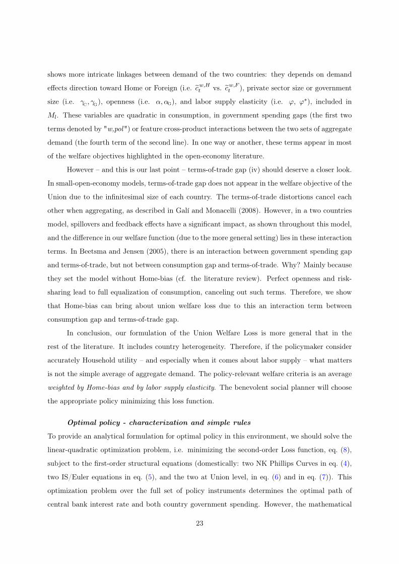
(iii) When central bank policy reacts with inertia: The slow pace of interest rate adjustment

on the short-run changes the dynamics, and this time, there is no consumption drop at the Union

level. Even more, the inflationary pressure and the slow pace of terms-of-trade adjustment lead

them to increase their consumption: as aggregate demand shift toward Foreign goods, inflation

rise. After several periods, with the adjustment of interest rate, both consumption and inflation

drop, especially for Home. As a result, the Foreign Household benefit again from the spending

shock when Central Bank takes time to adjust: for a similar level of inflation, the Foreign

consumption and output gaps are positive.

Figure 2: Response to a 1% spending shock

20 40 600

0.005

0.01

0.015Home spending shock

20 40 600

5

10 #10-4 Home inflation

20 40 60-2

0

2

4 #10-4 Foreign inflation

20 40 600

2

4

6 #10-4 Union inflation

20 40 60-1.5

-1

-0.5

0 #10-3 Terms of trade gap

20 40 600

2

4

6 #10-4 CB interest rate

20 40 60-2

-1

0

1

2 #10-3 Home cons. gap

20 40 60-2

-1

0

1

2 #10-3 Foreign cons. gap

20 40 60-1

-0.5

0

0.5

1 #10-3 Union cons. gap

20 40 600

1

2

3

4 #10-3 Home output gap

20 40 60-1

-0.5

0

0.5

1 #10-3 Foreign output gap

Inflation adverse responseSteady state (flexible price)Taylor rule responseInertial response

Fiscal shock & CB response

Public spending shock follows a AR(1) process, Central bank reacts to inflation under the rules detailedin table 2, and fiscal policy is passive after the shock, i.e. gt = g∗t = 0

30

In this type of model, the transmission of fiscal policy across the currency union depends exceed-

ingly on central bank mandate. This is also the case when we differentiate between "autarkic"

and "open" government spending. Previously, government spending was "autarkic", purchasing

only domestic goods, with a complete Home-bias (αG = αG* = 0). When considering an "open"

government (αG = αG* = 0.25, almost as open as private consumption), the main difference is the

extended transmission of inflation. Consequently, government demand affects directly the Foreign

NK-Philipps Curve. However, beside this minor difference, the dynamics are very much alike.

Concerning the role of central bank reaction for spillover effects, the main insight is analogous.

8 Structural heterogeneity: a rationale for policy cooperation

Our model presents heterogeneity in most parameters. Studying how it would affect spillovers

of Productivity or Government spending shocks is a long and monotonous task. Each parameter

may change slightly one particular channel, but a meticulous review would be mostly redundant.

However, some of the structural parameters – what we can call "supply-side factors" – are acting

in the same direction. In union-NKPC eq. (6), we collected them in a new parameter ξh for Home

and ξf for Foreign, defining it as ξh ≡ 2ΞHχϕγC

+ γC*

(and ξf ≡ 2ΞFχ∗ ϕ∗

γC

+ γC*

). It represents how structural

factors, such as labor supply elasticity, price rigidity and relative taste for Home/Foreign good,

affects inflation through the New-Keynesian Philipps Curve. More rigorously, low Frisch elasticity

(high ϕ), more flexible prices (low θ, high χ) and higher tastes for private goods (high ΞH), all

increases ξh, and, as a result, inflation at Home is relatively more reactive than in the Foreign

country. Such difference will have important implications for policy, and we try to provide a

succinct view on this issue. We use the following calibration19.

Table 3: Comparison and heterogeneity in structural parameters value

Parameter High value of ξ Low value of ξ Signification

ϕ 4 2 Inverse Frisch elasticityχ 0.012 0.007 Slope of NKPCθ 0.898 0.922 Price stickiness (measure of firms who can’t reset prices)Ξi 0.5 0.25 Union demand for Home goodα 0.2 0.3 Openness in private consumptionξi 0.064 0.0093 Inflationary effect of supply-side factors ξi ≡ 2Ξiχϕ

γC

+ γC*

19This calibration is motivated by empirical estimates: Frisch elasticity 1/ϕ vary between 0.25 and 0.5, whileestimate of the NKPC slope χ vary between 0.008 and 0.014. Our range of parameter value for calibration(0.007-0.012) can be justified by the absence of wages rigidities in this model

31

Figure 3: Response to a 1% productivity shock, comparison with two heterogeneous countries

10 20 30 400

0.005

0.01

0.015 Home TFP shock

10 20 30 40-8

-6

-4

-2

0

2 #10-4 Home inflation

10 20 30 40-2

0

2

4

6

8 #10-4 Foreign Inflation

10 20 30 40-4

-2

0

2

4 #10-4 Union inflation

10 20 30 40-10

-5

0

5 #10-3 Terms-of-trade gap

10 20 30 40-4

-3

-2

-1

0

1 #10-3 Home cons. gap

10 20 30 40-1

0

1

2

3

4 #10-3 Foreign cons. gap

10 20 30 40-2

-1

0

1

2 #10-4 Union cons. gap

10 20 30 40-10

-5

0

5 #10-4 CB interest rate

10 20 30 40-4

-3

-2

-1

0 #10-4 Natural rate

10 20 30 40-1

0

1

2

3 #10-3 Home gov. spending

10 20 30 40-3

-2

-1

0

1 #10-3 Foreign gov. spending

10 20 30 40-3

-2

-1

0

1 #10-3 Home output gap

10 20 30 40-1

0

1

2

3 #10-3 Foreign output gap

Optimal policy - high 9hSteady-state (flexible prices)Optimal policy - low 9h

Heterogeneous countries

TFP follows a AR(1) process. Countries have heterogeneous structural parameters, summarized byξh ≡ 2ΞHχϕ

γC

+ γC*. Monetary and fiscal policies are optimal (commitment). Results are shown in table 4

How heterogeneity affects the transmission of an asymmetric shock

As we discussed above, an asymmetric shock can have a very different impact on aggregate

variables depending on structural parameters. As we observe, an asymmetric productivity shock

have spillover effects on Union inflation and output gap and prevent central bank from following

Natural interest rate. We show two cases: in the first (a), Home economy has a high ξh and is

more affected by price changes: the deflationary episode it experiences after the supply-shock

have a faster influence on Union prices, which also adjust downward. Facing deflation at Union-

level, monetary policy reacts by cutting interest rate close to two time below the natural rate.

A contrario, in (b) when the Foreign country is more subject to inflationary pressure, the Union

inflation is pushed upward following the Home supply shock. This is because the terms-of-

trade gap worsen in favor of the Foreign country, which attracts the union aggregate demand.

32

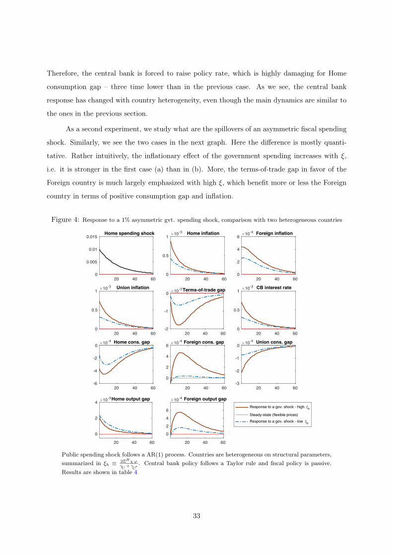
Therefore, the central bank is forced to raise policy rate, which is highly damaging for Home

consumption gap – three time lower than in the previous case. As we see, the central bank

response has changed with country heterogeneity, even though the main dynamics are similar to

the ones in the previous section.

As a second experiment, we study what are the spillovers of an asymmetric fiscal spending

shock. Similarly, we see the two cases in the next graph. Here the difference is mostly quanti-

tative. Rather intuitively, the inflationary effect of the government spending increases with ξ,

i.e. it is stronger in the first case (a) than in (b). More, the terms-of-trade gap in favor of the

Foreign country is much largely emphasized with high ξ, which benefit more or less the Foreign

country in terms of positive consumption gap and inflation.

Figure 4: Response to a 1% asymmetric gvt. spending shock, comparison with two heterogeneous countries

20 40 600

0.005

0.01

0.015 Home spending shock

20 40 600

0.5

1 #10-3 Home inflation

20 40 600

2

4

6 #10-4 Foreign inflation

20 40 600

0.5

1 #10-3 Union inflation

20 40 600

0.5

1 #10-3 CB interest rate

20 40 60-6

-4

-2

0 #10-4 Home cons. gap

20 40 60

0

2

4

6 #10-4 Foreign cons. gap

20 40 60-3

-2

-1

0 #10-4 Union cons. gap

20 40 60

0

2

4 #10-3 Home output gap

20 40 60

0

2

4

6

#10-4 Foreign output gapResponse to a gov. shock - high 9hSteady-state (flexible prices)Response to a gov. shock - low 9h

20 40 60-2

-1

0 #10-3 Terms-of-trade gap

Public spending shock follows a AR(1) process. Countries are heterogeneous on structural parameters,summarized in ξh ≡ 2ΞHχϕ

γC

+ γC*. Central bank policy follows a Taylor rule and fiscal policy is passive.

Results are shown in table 4

33

Table 4: Results: Spillovers of shocks, Welfare loss, Fiscal multipliers and country heterogeneity

Type of shock Parameter ξ Monetary Fiscal policy Welfare loss Fiscal multiplierHome Foreign response response Home Foreign

Home TFP shock High (0.064) Low (0.0093) Inflation rule Passive 0.012 NA NAHome TFP shock High (0.064) Low (0.0093) Optimal policy Optimal policy 0.010 0.956 0.3734Home TFP shock Low (0.0093) High (0.064) Optimal policy Optimal policy 0.010 0.3734 0.956Home fiscal shock High (0.064) Low (0.0093) Taylor rule Passive 0.038 0.643 NAHome fiscal shock Low (0.0093) High (0.064) Taylor rule Passive 0.034 0.617 NAUnion fiscal shock High (0.064) Low (0.0093) Taylor rule Passive 0.080 0.770 0.883

Notes: ◦ Central Bank follows a simple policy rule: i∗t = rnatt + φπ πw,t + φc cw,tOr it may react with inertia: it = ρi it−1 + (1− ρi) i∗t (with ρi = 0.95)

◦ Fiscal policy is either passive: gt = 0 or follows the optimal policy under commitment.◦ Welfare loss is expressed as percent of consumption◦ Government spending multiplier is measured as the ratio of integrals of output gaps over spending gaps◦ Calibration: Home (resp. Foreign) have either "low" (resp. high) or "high" (resp. low) parameter value ξh (resp. ξf )

How heterogeneity affects the transmission of an aggregate shock

This model was well suited to study asymmetric shock. However, heterogeneity in structural

parameters provides the two economies with different resilience to a common aggregate shock,

which, in turn, results in asymmetric spillovers. We should again study two types of common

shock: a productivity shock and spending shock.

Even though we do not show the graph, we argue that a common aggregate shock does not

produce asymmetric spillovers. As we described in eq. (7), the response to an aggregate shock

is simply a drop in natural interest rate and Central Bank nominal rate. This has an impact

on the Union-level Dynamic-IS equation, and this affects consumption at Home and Abroad

equally. Therefore, there is no spillover on inflation, neither in the individual countries, nor at

the Union-level. This is once more rooted in the Taylor principle, (and the "treat" of Central

Bank anti-inflation mandate). This is analogous to the simple "one country" NK model.

However, concerning a common (demand) fiscal common shock, the situation is very differ-

ent. We simulate a common fiscal shock, or equivalently a rise in government purchases affecting

both countries equally: the size of government is the same, and both fiscal shock are "autarkic":

AR(1) processes out of a passive fiscal mandate. This kind of experiment could be relevant, for

example, if the Currency Union is involved in a political conflict and should rise military spending

in all its region. The consequence is an asymmetric diffusion of inflation, higher in the region

with the highest parameter ξi. As we note in the following graph, when ξh is high, inflation is

higher at Home, even though government spending is the same, and this distorts terms-of-trade

for the benefit of the Foreign country, with a positive consumption gap.

34

Figure 5: Response to a 1% aggregate government spending shock, analysis with heterogeneity

20 40 600

0.005

0.01

0.015 Union spending shock

20 40 600

0.5

1

1.5 #10-3 Home inflation

20 40 600

0.5

1

1.5 #10-3 Foreign inflation

20 40 600

0.5

1

1.5 #10-3 Union inflation

20 40 60-2

0

2 #10-3 Terms of trade gap

20 40 600

0.5

1

1.5 #10-3 CB interest rate

20 40 60

-4

-2

0

2

#10-4 Home cons. gap

20 40 60

-4

-2

0

2

#10-4 Foreign cons. gap

20 40 60-3

-2

-1

0 #10-4 Union cons. gap

20 40 60

0

1

2

3 #10-3 Home output gap

20 40 60

0

1

2

3 #10-3 Foreign output gap

Response to an union shock - high 9hSteady-state (flexible prices)

Response to an union shock - low 9h

Spending shock follows a AR(1) process and hits both economies. Countries are heterogeneous on structuralparameters, summarized in ξh ≡ 2ΞHχϕ

γC

+ γC*. CB follows a Taylor rule and fiscal policy is passive.

Fiscal policy experiments – conclusion

There are plenty of policy experiments to be implemented. Concerning asymmetric fiscal shocks,

beside various types of spillovers, common characteristics remain. The general story is the

following: a fiscal shock brings about inflation and central bank reaction, worsening consumption

gap in the two countries. In different cases, the spillovers on Foreign consumption gap can be

positive: in such situation, Central Bank necessarily follows a rule that accounts for consumption

gap. When countries are heterogeneous, labor elasticity, openness and price flexibility change

quantitatively the transmission of inflation through terms-of-trade: Foreign country’ inflation

and consumption are much severely affected when structural parameter ξf is high. All these

experiments, as well as fig. 6 in appendix provide a clearer picture of the different effect on

welfare and fiscal multipliers and cross-country spillovers.

35

9 Conclusion

In this master thesis, we provided a two country DSGE model with "large economies" in a

monetary union. Our New-Keynesian framework emphasized the transmission channels due to

interactions between the two economies, their fiscal policies and a common central bank. In

particular, we allow for Home bias in consumption of private and public goods as well as for

heterogeneity in preferences and structural "supply-side" factors (share of goods production,

labor elasticity, price flexibility).

From this very general setting, we extracted many different results: we first determined the

cooperating optimal allocation at the first-best: private consumption and public spending should

follow the productivity of the two countries, weighted by structural preferences. Second, when

nominal rigidities exists, there exists policy trade-off, in terms of consumption gaps, inflation

and terms-of-trade gap. We determined how to achieve optimal policy by the mean of simple

rules: inflation rule for central bank policy and reaction to terms-of-trade and consumption gap

for fiscal authorities. Third, this environment was suitable to study many different experiments.

We analyzed the various implications of productivity and government spending shocks, and

spillover effects from one large country to the other. The reaction of the central bank is key

in this mechanism. An asymmetric positive supply shock (at Home), followed by a cut in the

union interest rate boost consumption and inflation in the Foreign country. An asymmetric

spending shock, a contrario, can create depression and deflation abroad if the central bank is

strongly inflation. Taylor-rule mandate, inertia in interest rate, "open"-government spending

and heterogeneity in country reliance to inflation can all induce more inflationary spillover in

the Foreign country. Finally, our model presented heterogeneity in most parameters and we

could study different policy implications. We could briefly note that fiscal policy effectiveness –

through government spending multipliers – can be greater when one country is more sensitive to

inflationary pressures.

This last observation brings about a key question: when one country experiences a supply or

demand shock, what are the gains from policy cooperation? We studied welfare gains when fiscal

policy was optimal – substantial gains due to labor inelasticity and trade imbalances between

the two countries. However, we did not study non-cooperative situations. For example, if Home

country experiences a supply shock, is the Foreign country willing to "help" the Home country

for stabilizing this shock? or would it "deviates" and let Home fiscal policy hold all the burden

of the fiscal adjustment? If we are able to compare the diverse outcomes, the answer to this

36

question would require an extended game-theoretical framework and in particular dynamic games

and recursive contracts. We consider this question relevant and would like to pursue on such

questions in the future.

There are plenty of different directions for future research: if the model included rather

heavy notations and cumbersome equilibrium relations (for the optimal policy) our framework

still abstracted from many features: realistic labor markets ; incomplete financial markets where

fiscal union could act as an insurance tool ; public sector with government debt and distortive

taxation, emphasizing the costs of policy intervention, and finally credit constraint and imperfect

consumption/saving decisions by households or firms. We plan to study some of these topics in

the future, in the context of monetary unions.

However, with our simple framework, we could describe many policy implications: we

showed the various transmission channels of supply and public demand shock, through cen-

tral bank reaction and trade spillovers, and how heterogeneity between the two countries could

transform an "asymmetric" issue – e.g. terms-of-trade or relative consumption gap – into an

"aggregate" one. This is a strong case for macroeconomic coordination between the national

fiscal authorities and the union central bank. We believe this article provide a clearer view on

these topics and can shed light on several policy issues in the context of European Union.

37

References

Adjemian, Stéphane, Houtan Bastani, Michel Juillard, Ferhat Mihoubi, George Perendia, Marco Ratto and

Sébastien Villemot (2011), ‘Dynare: Reference manual, version 4’.

Aguiar, Mark, Manuel Amador, Emmanuel Farhi and Gita Gopinath (2014), Coordination and crisis in monetary

unions, Working Paper 20277, National Bureau of Economic Research.

Baxter, Marianne and Robert G. King (1993), ‘Fiscal policy in general equilibrium’, The American Economic

Review 83(3), 315–334.

Beetsma, Roel and Henrik Jensen (2005), ‘Monetary and fiscal policy interactions in a micro-founded model of a

monetary union’, Journal of International Economics 67(2), 320 – 352.

Beetsma, Roel and Massimo Giuliodori (2011), ‘The effects of government purchases shocks: Review and estimates

for the eu*’, The Economic Journal 121(550), F4–F32.

Benigno, Pierpaolo (2004), ‘Optimal monetary policy in a currency area’, Journal of International Economics

63(2), 293 – 320.

Blanchard, Olivier, Christopher J Erceg and Jesper Lindé (2017), ‘Jump-starting the euro-area recovery: would

a rise in core fiscal spending help the periphery?’, NBER Macroeconomics Annual 31(1), 103–182.

Bordo, Michael D., Lars Jonung and Agnieszka Markiewicz (2013), ‘A fiscal union for the euro: Some lessons from

history’, CESifo Economic Studies 59(3), 449–488.

Carlino, Gerald A. and Robert P. Inman (2013), ‘Local deficits and local jobs: Can us states stabilize their own

economies?’, Journal of Monetary Economics 60(5), 517 – 530. Aggregate Implications of Local Public Finance.

Christiano, Lawrence, Martin Eichenbaum and Sergio Rebelo (2011), ‘When is the government spending multiplier

large?’, Journal of Political Economy 119(1), 78–121.

Correia, Isabel, Emmanuel Farhi, Juan Pablo Nicolini and Pedro Teles (2013), ‘Unconventional fiscal policy at

the zero bound’, The American Economic Review 103(4), 1172–1211.

Devereux, Michael B. (1991), ‘The terms of trade and the international coordination of fiscal policy’, Economic

Inquiry 29(4), 720–736.

Drautzburg, Thorsten and Harald Uhlig (2015), ‘Fiscal stimulus and distortionary taxation’, Review of Economic

Dynamics 18(4), 894 – 920.

Farhi, Emmanuel, Gita Gopinath and Oleg Itskhoki (2014), ‘Fiscal devaluations’, The Review of Economic Studies

81(2), 725–760.

Farhi, Emmanuel and Ivan Werning (2012a), Fiscal unions, Working Paper 18280, National Bureau of Economic

Research.

38

Farhi, Emmanuel and Iván Werning (2012b), Fiscal multipliers: Liquidity traps and currency unions, Working

Paper 18381, National Bureau of Economic Research.

Ferrero, Andrea (2009), ‘Fiscal and monetary rules for a currency union’, Journal of International Economics

77(1), 1 – 10.

Frankel, Jeffrey A and Katharine Rockett (1988), ‘International macroeconomic policy coordination when policy-

makers disagree on the model’, American Economic Review 78(3), 318–340.

Galí, Jordi and Tommaso Monacelli (2005), ‘Monetary policy and exchange rate volatility in a small open econ-

omy’, The Review of Economic Studies 72(3), 707–734.

Galí, Jordi and Tommaso Monacelli (2008), ‘Optimal monetary and fiscal policy in a currency union’, Journal of

International Economics 76(1), 116 – 132.

Galí, Jordi, J. David López-Salido and Javier Vallés (2007), ‘Understanding the effects of government spending

on consumption’, Journal of the European Economic Association 5(1), 227–270.

Gordon, Roger H. (1983), ‘An Optimal Taxation Approach to Fiscal Federalism’, The Quarterly Journal of

Economics 98(4), 567–586.

Hebous, Shafik and Tom Zimmermann (2013), ‘Estimating the effects of coordinated fiscal actions in the euro

area’, European Economic Review 58, 110 – 121.

Kehoe, Patrick J (1987), ‘Coordination of fiscal policies in a world economy’, Journal of Monetary Economics

19(3), 349–376.

Liu, Zheng and Evi Pappa (2008), ‘Gains from international monetary policy coordination: Does it pay to be

different?’, Journal of Economic Dynamics and Control 32(7), 2085 – 2117.

Michau, Jean-Baptiste (2014), Monetary and Fiscal Policy in a Liquidity Trap with Inflation Persistence. working

paper or preprint.

Oates, Wallace E. (1999), ‘An essay on fiscal federalism’, Journal of Economic Literature 37(3), 1120–1149.

Poghosyan, Tigran, Abdelhak Senhadji and Carlo Cottarelli (2014), ‘The role of fiscal transfers in smoothing

regional shocks’, Designing a European Fiscal Union: Lessons from the Experience of Fiscal Federations 34, 60.

Smets, Frank and Raf Wouters (2003), ‘An estimated dynamic stochastic general equilibrium model of the euro

area’, Journal of the European Economic Association 1(5), 1123–1175.

Wildasin, David E (1988), ‘Nash equilibria in models of fiscal competition’, Journal of public economics 35(2), 229–

240.

Wilson, John D. (1986), ‘A theory of interregional tax competition’, Journal of Urban Economics 19(3), 296–315.

39

Appendices

Structural parameters – heterogeneity and restrictions

In this model, we refer to a number of structural parameters. The definitions and how the diverse hypothesis

constrained the range of their value is referenced in the following list:

• Demand parameters:

α Share of foreign goods in Household consumption bundle, indice of "openness" [α 6= α∗] ; αG Share

of foreign goods in government spending, indice of "government openness" [αG 6= αG*] ; Γ Preference of

Household for public goods: [Γ 6= Γ∗] ; ε Elasticity of substitution across varieties of goods

γC , γC*, γG , γG* respectively, share of Home consumption, Foreign consumption, Home government spending,

Foreign government spending, in union aggregate demand ;

ω ≡ (1 − α)αγC +(1 − α∗)α∗ γC* +(1 − αG)αG γG +(1 − αG*)αG* γG*. It represents how demand for Home-

goods increases with a terms-of-trade depreciation (st > 0 ), and by symmetry it also shows how demand

for Foreign goods is dampened following the same depreciation. [ω = ω∗] It increases in openness of the

different agents, and equals zero in complete autarky ;

ΞH ≡ (1− α) γC +α∗ γC* and ΞF ≡ (1− α*) γ

C* +αγC Share of Home/Foreign-goods in union consumption

• Supply parameters:

ϕ Disutility of labor, inverse of the Frisch Elasticity [ϕ 6= ϕ∗] ; θ Degree of price stickiness [θ 6= θ∗] ; χ How

inflation reacts to a rise in marginal costs: χ = (1− θ)(1−βθ)/θ, decreasing in price stickiness and infinite

in flexible prices [χ 6= χ∗]

η = (1− Γ)(1− α) + (1− Γ∗)α∗ + Γ(1− αG) + Γ∗ αG* represents agent preferences for Home goods, and

as a result, is related to the structural labor supply at optimum N = ηϕ

1+ϕ and similarly for the foreign

country: η∗ ≡ (1− Γ∗)(1− α∗) + (1− Γ)α+ Γ∗(1− αG*) + ΓαG

ξh ≡ 2ΞHχϕγC

+ γC*

and similarly ξf ≡ 2ΞFχ∗ ϕ∗

γC

+ γC*

represents "supply-side" factors influencing the resilience of a

country to inflationary demand shocks.

• Parameters restrictions – assumptions

1. Equal size of the two countries, Y = Y ∗ = 1/2Yw, therefore shares of the different part of the economy

at steady-state are constrained as follow:

1/2 = γC(1− α) + γC* α

∗ + γG (1− αG) + γG* αG* = ΞH + γG (1− αG) + γ

G* αG*

= γC*(1− α*) + γC α+ γ

G* (1− αG*) + γG αG = ΞF + γG* (1− αG*) + γG αG

2. Risk-sharing condition implies that consumption is equalized, modulo terms-of-trade differences.

Holding at steady-state we therefore have this null long-run trade balance.

γC = ΞH & γC* = ΞF this implies α∗ γ

C* = αγC

3. Structural preferences yield an unitary labor supply η, we thus have a necessary condition for pref-

erence homogeneity of the form:

(α∗ − α) + Γ(α− αG) = Γ∗(α∗ − αG*)

40

Equilibrium relations with policy trade-offs

• Definition of terms of trade gaps:

∆st = πF,t − πH,t − (∆at −∆a∗t )

• Evolution of exogenous productivity shocks as AR(1) process

at+1 = ρa at + εat & a∗t+1 = ρa a∗t + εa

∗t

• Evolution of exogenous fiscal shocks as AR(1) process

f εt+1 = ρf fεt + εft & f∗εt+1 = ρf f

∗εt + εf∗t

• Evolution of monetary policy and natural interest rates:

it = ρi it−1 + (1− ρi) (rnatt + φπ πw,t + φc cw,t)

rnatt = ρ+ 1γC

+ γC*

[ΞH Et(∆at+1) + ΞF Et(∆a

∗t+1)

]• Fiscal policy rules

gt = −1/2ψs st − ψc ct + f εt & g∗t = +1/2ψ∗s st − ψ∗c c∗t + f∗εt

• Domestic New Keynesian Philipps Curve equation, at Home and in the Foreign country:

πH,t = β Et πH,t+1 + χ[1 + 2ΞH ϕ

]ct + 2χϕ

{(1− αG) γG gt + αG* γG* g

∗t

}+

χ[α+ 2ϕ(ω − α∗ γ

C*(1− α− α∗))]st

πF,t = β Et πF,t+1 + χ∗[1 + 2ΞF ϕ∗

]c∗t + 2χ∗ϕ∗

{(1− αG*) γ

G* g∗t + αG γG gt

}− χ∗

[α* +2ϕ∗(ω − αγC(1− α− α∗))

]st

• Union-level Philipps Curve

πw,t = β Et πw,t+1 + ΞH( χγC

+ γC*

+ ξh)ct + ΞF

( χ∗

γC

+ γC*

+ ξf)c∗t

+ γG{

(1− αG)ξh + αG ξf}gt + γ

G*

{(1− αG*)ξf + αG* ξh

}g∗t

+[

αγC

γC

+ γC*

(χ− χ∗) + (ξh − ξf )]st+1

• Domestic Euler equation, at Home and in the Foreign country:

ct = Et ct+1 − (it − rnat) + Et πw,t+1 −γC* (1−α−α*)

γC

+ γC*

Et ∆st+1

c∗t = Et c∗t+1 − (it − rnat) + Et πw,t+1 +

γC

(1−α−α*)

γC

+ γC*

Et ∆st+1

• Union-level Euler equation

cw,t = Et cw,t+1 − {(γC + γC*)[it − rnat]− (ΞH Et πH,t+1 + ΞF Et πF,t+1)}

41

Welfare, fiscal multiplier and effectiveness of optimal policy in

function of structural parameters

Figure 6: Results in terms of structural parameters

This graph displays the effectiveness of fiscal of policy in optimal policy – compared to thepassive situation – using two criterions: first the fiscal multiplier (output response to spending -orange) and second the relative loss (yellow) of the welfare loss in the non-intervention scenariocompared to optimum – and the welfare loss as the optimum (blue). These graph examine thesensitivity of these variables to change in (i) openness, (ii) price stickiness, (iii) labor supplyelasticity.For instance, the left graph displays that at the benchmark calibration (red dot) the fiscalmultiplier is 0.7, the welfare loss (blue) at optimum corresponds to 0.005% of consumption(very small!) and that the loss under passive policy is 2 times higher. When country is fullyopen α = 0.5, with more flexible prices (high χ) or labor supply is rigid (small Frisch elasticity),there is a smaller welfare loss at optimum and the fiscal multiplier is smaller (0.6 instead of0.7-0.8). Fiscal policy is particularly effective (in terms of welfare), when labor supply is rigidas it balances the labor demand between the two countries.

42

Figure 7: Results in terms of structural parameters

This graph displays the effectiveness of fiscal of policy in optimal policy – compared to thepassive situation – using two criterions: first the fiscal multiplier (output response to spending- orange for Home country, green for Foreign) and second the relative loss (yellow) of thenon-intervention scenario compared to optimum – and the welfare loss as the optimum (blue).These graph examine the sensitivity of these variables to change in (i) openness, (ii) pricestickiness, (iii) labor supply elasticity.The multipliers of the two countries are inversely related: for instance when Home is less openthan Foreign, its multipliers is substantially greater. In all graphs, the fiscal policy is moreeffective in terms of welfare when the two countries are asymmetric, i.e. the welfare loss is 70%higher when the policy is absent when the differential between the two countries is high.

Derivation of the Welfare-function

In this section, we state the Household utility function, approximated at the second order. The formula

is heavy due parameters heterogeneity. The various multiplicative factors are induced by interactions

between the two countries (structural parameters γi representing the weights of the aggregates in the

"Union economy"). Also, variable zt represents the usual New-Keynesian’s style price dispersion i.e.

zt ≡ ln∫ 1

0

(PH,t(i)PH,t

)−εdi.

43

U(Ct, Gt, Nt) = (1− Γ) ln(Ct) + Γ ln(Gt)− N1+ϕt

1+ϕ

' (1− Γ) ct + Γ gt − zt − 2[(1− α) γC ct + α* γC* c

∗t + (1− αG) γG gt + (1− αG*) γ

G* g∗t + ωst]

−((1−α) γ

C+2ϕ(1−α)2 γ

C2)

(ct)2 −

(α* γ

C* +2ϕα*2 γC*

2)

(c∗t )2

−((1−αG) γ

G+2ϕ(1−αG)2 γ

G2)

(gt)2 −

(αG* γG* +2ϕαG*

2 γG*

2)

(g∗t )2

−(ν+2ϕω2

)s 2t −

((1−α) γ

C(2α+4ωϕ)

)ct st −

(α* γ

C*(2(1−α*)+4ωϕ))c∗t st

−((1−αG) γ

G(2αG +4ωϕ)

)gt st −

(αG* γG*(2(1−αG*)+4ωϕ)

)g∗t st

− 4ϕ[(

(1−α) γCα* γ

C*

)ct c

∗t −

((1−α) γ

C(1−αG) γ

G

)ct gt −

((1−α) γ

CαG* γG*

)ct g

∗t

−(α* γ

C*(1−αG) γG

)c∗t gt −

(α* γ

C* αG* γG*

)c∗t g

∗t −

((1−αG) γ

C* αG* γG*

)gt g

∗t

]

We obtain a similar formula for the Foreign Household, replacing parameters by their "∗" equivalent, and

st by −st. We observe that this second order approximation includes first-order terms. Hopefully, these

terms cancel out when we consider the Union as a whole. This is because, as discussed in first section of

appendices (parameters restrictions), we have Γ = 2 γG and Γ∗ = 2 γG*. Therefore, we rewrite the loss

function as the negative utility:

Lwt = −Ut(Ct, Gt, Nt)− U∗t (C∗

t , G∗t , N

∗t )

= −(1− Γ) ln(Ct)− Γ ln(Gt) +N1+ϕ

t

1+ϕ − (1− Γ∗) ln(C∗t )− Γ∗ ln(G∗

t ) +N

∗(1+ϕ∗)t

1+ϕ∗

' zt + z∗t + [γCc 2t + γ

C* c∗ 2t + γ

Gg 2t + γ

G* g∗ 2t + ωs 2

t ]

+ 4 γCω((1−α)ϕ−αϕ∗) ctst + 4 γ

C* ω(α*ϕ−(1−α*)ϕ∗) c∗t st

+ 4 γGω((1−αG)ϕ−αG ϕ∗) gtst + 4 γ

G* ω(αG ϕ−(1−αG*)ϕ∗) g∗t st

+ 2 γC

2((1−α)2ϕ+α2ϕ∗) c 2t + 2 γC*

2(α*2 ϕ+(1−α*)2ϕ∗) c∗ 2t

+ 2 γG

2((1−αG)2ϕ+αG2 ϕ∗) g 2

t + 2 γG

2(αG*2 ϕ+(1−αG*)2ϕ∗) g∗ 2

t +

+ 2 γCγC*((1−α)α*ϕ+α(1−α*)ϕ∗) ct c

∗t + 2 γ

CγG((1−α)(1−αG)ϕ+ααG ϕ

∗) ct gt

+ 2 γCγG*((1−α)αG ϕ+α(1−αG)ϕ∗) ct g

∗t + 2 γ

C* γG (α*(1−αG)ϕ+(1−α)αG ϕ∗) c∗t gt

+ 2 γC* γG*(α*αG ϕ+(1−α*)(1−αG*)ϕ∗) c∗t g

∗t + 2 γ

GγG*((1−αG)αG*ϕ+αG(1−αG*)ϕ∗) gt g

∗t

As we see, this formula is rather cumbersome. Rearranging the terms, it is possible to express the Loss

function with vectors, and obtain a more compact formula, as shown in eq. (8). More, as shown in Galí

and Monacelli (2008), the term representing the price dispersion zt can be expressed as the square of

inflation.

44