Fiscal Policy and the Current Account

S. M. Ali Abbas, Jacques Bouhga-Hagbe, Antonio Fatás, Paolo Mauro, and Ricardo C. Velloso1

May 2011

Abstract

This paper examines the relationship between fiscal policy and the current account, drawing on a large sample of advanced, emerging and low-income economies and using a variety of statistical methods: panel regressions, an analysis of large fiscal policy and current account changes, and panel vector auto-regressions. On average, a strengthening in the fiscal balance by 1 percentage point of GDP is associated with a current account improvement of 0.3-0.4 percentage point of GDP. This association appears stronger in emerging and low-income economies; when the exchange rate is flexible (although this result does not survive in vector auto-regressions); the economies are more open; output is above potential; initial debt levels are above 90 percent of GDP; and using methods more robust to endogeneity issues. JEL Classification Numbers: E60, E61, E62, E65, C40, C01 Keywords: fiscal policy, external imbalances, current account, exchange rate Authors’ e-mail addresses: sabbas@imf.org, jbouhgahagbe@imf.org, antonio.fatas@insead.edu,

pmauro@imf.org, rvelloso@imf.org

1 The authors are grateful to Carlo Cottarelli for suggesting the topic and constructive comments, the IMF Economic Review editor and two anonymous referees, Philip Gerson and participants in the workshop on External Imbalances and Public Finances at the European Commission, November 2009 for helpful comments; and Junhyung Park for outstanding research support. Abbas, Mauro, and Velloso are in the IMF’s Fiscal Affairs Department. Bouhga-Hagbe is in the IMF’s Western Hemisphere Department. Fatás is Professor of Economics at INSEAD.

2

I. INTRODUCTION The relationship between fiscal policy and the current account has long attracted interest among academic economists and policymakers alike, from various angles. For example, the possible link between fiscal deficits and current account deficits has spurred many studies analyzing the “twin deficit” hypothesis, particularly for the case of the United States. For countries where current account imbalances are especially large, a relevant question has been to what extent fiscal adjustment can contribute to resolving external imbalances. Going forward, the implications of fiscal stimulus first, and fiscal adjustment later, for current account developments will no doubt continue to generate interest in the context of returning the global economy to strong, sustainable, and balanced growth as the effects of the 2008–09 crisis gradually abate. This paper analyzes the relationship between fiscal policy and the current account. The paper’s main contribution is in the breadth of its empirical investigation, in terms of both country coverage and variety of empirical techniques. Our sample includes about a hundred countries over several decades. The estimates distinguish among advanced and emerging/low-income countries; more and less open economies; fixed and floating exchange rate regimes, and country-years with small and large output gaps.2 To get a preview of the data, the paper begins with a series of panel regressions to generate broad estimates of the association between the current account and fiscal policy, the latter proxied by the cyclically-adjusted primary balance. The regressions also help identify factors affecting this association, such as exchange rate regime, level of financial and trade openness, whether the economy is below or above potential, level of initial public debt, and the revenue-expenditure mix of fiscal policy. This exercise is followed by an analysis of large changes in fiscal policy and the current account, using the well-known saving-investment accounting identity and event study methods, with a view to informing ongoing debates about the possible role of fiscal consolidation in correcting large imbalances in current-account deficit countries. The paper concludes with panel vector auto-regressions (VARs) using both annual and quarterly data in order to address endogeneity issues in our previous anslysis. The findings vary across techniques, yielding responsiveness estimates around 0.3 in the panel regressions and annual panel VARs, and 0.4-0.5 for the quarterly panel VARs. This association is stronger in emerging and low-income countries, more open economies, with flexible exchange rates, when output above potential or when initial debt levels are above 90 percent of GDP. These results suggest that changes in fiscal policy are indeed associated with changes in the current account, but the relationship is far less than one-for-one. In addition, the analysis of large episodes reveals a smaller responsiveness of the current account (in the range 0.1-0.2) and, for the most part, the emergence or unwinding of large current account imbalances is not closely associated with fiscal policy changes. The use of a range of techniques is important, given the unavoidable tradeoffs involved with any single methodology, sample of countries, or definition of fiscal policy. For example, studying the saving-investment accounting identity permits the inclusion of a large number of countries, but is subject to endogeneity concerns. The latter is attenuated with the use of cyclically-adjusted primary balances, but these raise other issues relating to the measurement of tax elasticities and potential output. Structural vector autoregressions with quarterly data on government

2 The paper is primarily analyzes association between changes in overall fiscal policy and the current account for an individual country. It does not delve into questions about the global transmission of fiscal policy shocks.

3

consumption can help avoid both endogeneity and measurement issues, while allowing a large sample of countries, but provide only a partial view of fiscal policy, by ignoring the tax side. By generating results across a spectrum of methods and samples, the paper provides insights that are more robust than those gleaned exclusively from one method. The rest of the paper is organized as follows. Section II reviews the theoretical and empirical literature. Section III presents results from the panel regressions. Section IV documents the relationship between fiscal and external balances for episodes of large changes in these balances. Section V reports the findings of the panel VAR analysis. Section VI concludes.

II. REVIEW OF THEORETICAL AND EMPIRICAL STUDIES Theoretical studies Fiscal policy and the current account are generally described as being bound by the following well-known identities:

CA = X () – M (Y,) + TP (1) CA = (Sp – Ip) + (Sg – Ig) (2)

where CA is the current account, X is exports of goods and services (decreasing in the real exchange rate, , where a higher denotes appreciation), M is imports of goods and services (decreasing in , but increasing in the national income, Y), and TP is transfer payments (remittances, net interest and profit receipts). Sp and Ip are private savings and investment, respectively; Sg and Ig are government savings and investment, so that Sg – Ig is equivalent to the government saving-investment balance (or fiscal balance, if there are no government transfers to the private sector). (1) and (2) also broadly describe the two major causal channels from fiscal policy to the current account, relating, respectively, to:

- Intratemporal trade (relative price changes): this channel works through the compositional effects of fiscal policy on aggregate demand—i.e. whether a fiscal policy change raises the demand for domestic (or nontradable) goods relative to foreign (or tradable) goods—and the impact thereof on the real exchange rate (the relative price of home to foreign goods) and the trade balance. Thus, increases in government spending (tax or debt-financed) if skewed towards home (or non-tradable goods), appreciates the real exchange rate and worsens the trade balance. The channel is highlighted well by both the Mundell-Fleming (1960) and dependent economy models (a la Salter, 1959).

- Intertemporal responses: this channel abstracts from differentiated goods and real

exchange rate misalignments, focusing instead on the intertemporal response of private agents to a given fiscal policy action in a one-commodity world. Now, a debt-financed fiscal impetus that seeks to worsen the trade balance, induces forward-looking agents to impute to their permanent incomes the offsetting future tax increases consistent with intertemporal government solvency. Hence, labor supply rises while private consumption falls, both effects seeking to improve the trade balance and pushing the economy towards a Ricardian outcome. The channel is articulated well in Obstfeld and Rogoff (1996) and Frenkel and Razin (1996).

4

The Mundell-Fleming (MF) model highlights well the workings of the relative price channel for a small open economy, as well as the importance of variables such as trade and financial openness, and monetary/exchange rate regime in determining the current account impact of fiscal policy changes. Under a flexible exchange rate regime, an expansionary fiscal shock raises the demand for home goods and money, inducing a nominal and real appreciation (effected via higher interest rates and arbitrage capital inflows) that crowds out net exports. However, if the capital account is relatively closed, a more enduring increase in interest rates results, crowding out investment, raising private savings, and thus softening the impact on the currency and trade balance. Under a fixed exchange rate regime, the central bank’s monetary accommodation in response to interest-rate-seeking capital inflows would reinforce the output multiplier while mitigating the net exports crowding out effect. However, this result hinges on whether and for how long a real appreciation can be forestalled via unsterilized (or even sterilized) interventions. In contrast to the relative price approach described above, intertemporal approaches take a longer-run view, and casting the current account as the excess of current domestic production over current domestic consumption of a single homogenous worldwide good (Frenkel and Razin, 1996). A key assumption in these forward-looking micro-founded models is that agents take into account future events in their current decisions (agents are Ricardian or near-Ricardian). An increase in debt-financed government spending, in this framework, works through the “future” to induce a higher saving and work effort response from private agents “today”: agents can foresee that the government must raise future taxes in order to offset the current fiscal deficit and ensure intertemporal solvency; these tax increases reduce the present value of future income (human wealth) and thus induce lower private consumption and higher labor supply in the present. The latter also raises the marginal product of capital, crowding in private investment. The current account deteriorates as long as the private saving increase (net of higher investment) does not offset the decline in public savings (Baxter, 1995). Risk premia also become important with forward-looking agents concerned about intertemporal solvency. Depending on whether the fiscal policy change under consideration exacerbates or attenuates debt sustainability concerns, a fiscal expansion can be contractionary or a fiscal contraction expansionary (Giavazzi and Pagano, 1990; 1996). In both eventualities, the fiscal policy-current account association weakens. New open economy models developed recently incorporate both the intertemporal and intratemporal dimensions as well as other advanced features such as risk premia, imperfect competition, sticky prices and policy reaction functions in an attempt to reconcile empirical puzzles found in the data: private consumption rising, real exchange depreciating (despite the trade balancing worsening) in response to a positive government spending shock. Perotti and Monacelli (2007) argue that private consumption could indeed rise in response to a government spending shock if agents needed to consume more to compensate for the misery of working harder and agents were unwilling to tilt consumption towards the future (small intertemporal elasticity of substitution). The real exchange rate depreciation is explained through international risk-sharing in complete financial markets;3 while the worsening of the trade balance occurs if consumption of foreign goods is relatively insensitive to the real depreciation (intratemporal elasticity of substitution between home and foreign goods is low). Ravn et al (2007) offer an

3 The marginal rate of substitution between the home and foreign country private consumption must be mirrored by the real exchange rate. Thus, a rise in current home private consumption (relative to the rest of the world) implies a real depreciation of the home currency.

5

alternative explanation for currency depreciation, grounded in deep habits: higher demand following the government spending shock induces firms to lower their markups to capture market share, thus, depreciating the domestic currency. Finally, Lane (2010) contends that “news that induces the government to provide fiscal impetus may also lead to a sell-off in currency markets.” Empirical Studies Previous empirical studies have generally found evidence suggesting that fiscal expansions worsen the current account. Estimates of the impact of 1 percentage point of GDP increase in the government deficit on the current account range between 0.2–0.7 percentage point of GDP, depending on the sample and techniques used (Appendix I). A few studies (mostly for large advanced economies) have also addressed the impact of fiscal policy on the real exchange rate, finding mixed effects. The methodologies used can be broadly grouped into three categories. The first category studies the impact of fiscal policy on external imbalances using causality tests and VARs. The second category analyzes the long-term correlation between indicators of fiscal policy and external imbalances, using cointegration techniques, and single or panel regressions techniques. The third category invokes the narrative approach to identify exogenous changes in fiscal policy and uses regression analysis to study their impact on external imbalances. The rest of this section presents a few key recent studies for each category, with the remaining studies summarized in Table 1. VAR Studies Studies using VARs have primarily looked at small samples of advanced economies. An important methodological choice in this setup is how to identify exogenous fiscal shocks. The preferred method in recent studies (e.g., Monacelli and Perotti, 2007; Beetsma et al, 2007) is to use changes in the log of real government consumption, because this measure is less affected by changes in GDP than is the case for alternatives such as the overall deficit/GDP ratio or the ratio of real government consumption to GDP. Indeed, this measure will also be used in the panel VAR section of this paper. On the whole, these studies have generally found evidence consistent with a small negative impact of fiscal expansions on the current account balance, except in large economies (like the United States), where the results are more mixed. For selected EU countries, Beetsma et al (2007) find that a government spending innovation of 1 percentage point of GDP worsens the trade balance by 0.5 percentage point of GDP upon impact and by 0.8 after two years. The real effective exchange rate appreciates (after a year), suggesting that the main short-term transmission channel upon impact is output, with the real exchange rate playing a greater role over longer horizons. For the United States, Monacelli and Perotti (2007) find that, following an increase in real government consumption by 1 percentage point of GDP, the trade balance stays around trend initially, but improves by 0.5 percentage points after about 3 years. They find stronger evidence in support of the twin deficits hypothesis (albeit only on impact) in the United Kingdom, Australia, and Canada. Similar results are obtained for the same countries by Corsetti and Muller (2006), who point out that the impact of fiscal shocks on the current account seems to be greater and longer-lasting in economies where total trade is higher as a share of GDP (Canada and the United Kingdom) than in economies where trade is a smaller share of GDP (US and Australia). Long-term Correlations and Panel Regressions

6

Studies involving large panels of countries are relatively rare. They are usually based upon panel regressions and find a statistically significant impact of fiscal variables on external imbalances. Abiad, Leigh, and Mody (2009) study determinants of the current account (in percent of GDP) for 135 countries (over 1975-2004) using a battery of random effects GLS regressions, and report a coefficient of 0.3 on the fiscal balance regressor (in percent of GDP) for the full sample. Mohammadi (2004) finds, for a sample of 20 advanced and 43 emerging and developing economies that a tax-financed spending increase is associated with a current account worsening of 0.16-0.29 percent of GDP (0.23-0.32 percent of GDP for developing countries, and 0-0.26 for advanced economies). If the spending is bond-financed, the current account balance worsens by 0.45-0.72 percent of GDP (0.55-0.81 percent of GDP for developing countries, and 0.22-0.50 for advanced economies). His estimated coefficients imply broadly symmetrical impact for fiscal expansions and contractions. Other important studies include IMF (2008), which applies panel techniques to both developing and advanced economies and finds that a 1 percentage point of GDP increase in government consumption is associated with an appreciation of the equilibrium real exchange rate of 2.5 to 3 percent. The actual impact on the current account could vary depending on the dynamic adjustment path of the actual real exchange rate toward the equilibrium; large current account worsenings can obtain if the real exchange rate appreciates above its equilibrium level (overshooting). Khalid and Guan (1999) use cointegration techniques in selected countries and find that the empirical evidence does not support any long-run relationship between the current account deficit and the fiscal deficit for advanced economies, while the data for developing countries does not reject such a relationship. However, their results suggest a causal relationship between the fiscal and current account balances for most countries in their sample, running from the budget balance toward the current account balance. Narrative Approach Romer and Romer (2007) investigate the impact of exogenous changes in the level of taxation on economic activity in the U.S. They use the narrative record, presidential speeches, executive-branch documents, and Congressional reports to identify the size, timing, and principal motivation for all major postwar tax policy actions. This narrative analysis allows them to distinguish tax policy changes resulting from exogenous legislative initiative (aimed, for example, at reducing an inherited budget deficit, or promoting long-run growth) from changes driven by prospective economic conditions, countercyclical actions, and government spending. Their estimates indicate that exogenous tax increases are highly contractionary, largely via a powerful negative effect on investment. Insofar as investment spending is an important current account determinant, the results point to a strong association between fiscal contraction and current account improvements. Using Romer-Romer data, Feyrer and Shambaugh (2009) estimate that one dollar of unexpected tax cuts in the U.S. worsens the U.S. current account deficit by 47 cents. A more recent dataset by Devries et al (2011) expands the narrative approach to identify action-based consolidations in 15 advanced economies. Evidence from that dataset suggests that the current account responds strongly to fiscal consolidation; implied response ratio is about 0.6 (Leigh et al, forthcoming). As the work is, as yet, unpublished, it is not possible to comment on the robustness of this result, and the extent to which it can be extrapolated to a larger group of countries.

7

III. PANEL REGRESSIONS OF CURRENT ACCOUNT ON FISCAL BALANCE We begin our empirical analysis with panel regressions on 88 non-oil exporting economies spanning the period 1970-2007.4 The distinction between advanced (30 countries) and emerging and low-income countries (58) is as per the IMF Fiscal Monitor (April 2011). The two key variables, the current account-to-GDP ratio and the cyclically-adjusted primary balance-to-potential GDP ratio, are derived from the IMF’s World Economic Outlook database (see below on derivation). Data quality was checked through reconciliation with IMF staff reports (with regard to the saving investment identity). For most advanced economies, the coverage starts from 1970; however, data on transition economies and many emerging and low-income economies is available for the post-1990 period only. The analysis discriminates country-years across several dimensions:

- Trade and financial openness: Trade openness is measured by the sum of imports and exports of goods and services (as a share of GDP), all from the WEO database. Financial openness is drawn from the Lane and Milesi-Ferretti (2006) dataset on the wealth of nations (2008 update) and defined as the sum of gross foreign financial assets and liabilities divided by GDP.

- Exchange rate regime: We use the IMF’s Annual Report on Exchange Arrangements and Exchange Rates classifications going back to 1990. The Report categorizes countries from 1 (“dollarized”) through 8 (fully floating). For our purposes, we include categories 1 through 3 (3 being adjustable peg) as fixed, and 7-8 (7 being managed float) as floating.

- Level of public indebtedness: We use the Abbas et al (2010) dataset on annual public debt-to-GDP ratios, effectively covering the entire IMF membership over 1970-2009.

- Output gap: This is defined as the percentage excess of actual over potential output, with the latter estimated using the Hodrick-Prescott filter. The output gaps were combined with a standard 1/0 elasticity assumption for revenues/expenditures to compute the cyclically-adjusted primary balance-to-GDP ratio, the main regressor.

The choice of the cyclically-adjusted primary balance-to-potential GDP ratio (CAPB) as the preferred measure of fiscal policy, as opposed to the headline fiscal balance, reflects the need to address the endogeneity problem that arises because shocks to the regressand (current account), especially due to growth, may be strongly correlated with headline fiscal balances.5 The resulting estimation bias is generally expected to be negative in advanced economies, with faster growth typically driving higher imports (weaker current accounts) and favorable automatic stabilizers and countercyclical fiscal policy (stronger headline balance). Denominator effects due to GDP scaling further aggravate this bias. In emerging and low-income countries, the direction of the bias is less easy to predict. Indeed in export-led economies, growth shocks would imply a co-movement in fiscal and external balances. Alternatively, financing constraints accompanying say, an adverse growth shock, could induce corrections in both fiscal and current account deficits.

4 In this section we restrict the analysis to non-oil exporting economies partly because of the strong association between the fiscal balance and the current account due to oil price changes simultaneously impacting tax revenues and exports but also because of data availability: the use of cyclically-adjusted primary balance reduces the sample of countries.

5 The cyclical adjustment was done using (i) an output gap measure obtained from HP filtering the real GDP series from the April 2009 vintage of the WEO database (smoothing parameter of 6.25); and (ii) an assumption that taxes/primary spending respond with a 1/0 elasticity to the output gap.

8

The choice of CAPB (which is scaled to potential GDP), while raising measurement issues in relation to tax elasticities and the output gap, helps attenuate the “automatic stabilizer and denominator” components of the bias noted above. Although the third component, which concerns the endogeneity of fiscal policy remains uncorrected, recent studies suggest that counter-cyclical fiscal policy is not the norm in Europe (Beetsma et al, 2009) while action-based fiscal consolidations in advanced economies, more generally, are at least as likely to happen in bad times as in good ones (Devries et al, 2011). This is particularly plausible in cases where weaker growth reveals underlying structural fiscal laxity and/or places binding financing constraints; the recent experience of peripheral European countries and emerging markets and low-income countries from earlier crises tends to support this view. Moreover, insofar as fiscal policy is subject to implementation lags, the share of say, a counter-cyclical fiscal expansion that is observed in the year in which the negative growth shock occurred, would likely be significantly less than 1. Overall, therefore, while we expect some endogeniety bias, we do not, a priori, expect to be large or systematically skewed in one direction. The regression results, obtained used fixed effects, are summarized in Table 1.6 The findings suggest that, on average, a strengthening in the cyclically-adjusted primary balance-to-potential GDP ratio (CAPB) of 1 percentage point is associated with an improvement in the current account-to-GDP ratio of about 0.3. The impact varies intuitively depending on the country-year characteristics noted above.

6 A constant and lagged per capita PPP GDP (from the World Economic Outlook database) were included in all regressions, while observations where the absolute value of the current account ratio or the CAPB ratio was above 20 percentage points were dropped.

9

1 2 3 4 5 6 7 8 9 10

Headline

regression

EMLICs vs

ADV

Trade

openness

Exchange

rate regime

FxER &

financial

openness

FLER &

financial

openness Output gap

Initial public

debt

Revenue

share in

fiscal

expansions

Revenue

share in

fiscal

contractions

0.049*** 0.036** 0.025 0.044 0.02 0.08 0.027 0.016 -0.017 0.039

[0.017] [0.018] [0.017] [0.043] [0.068] [0.055] [0.018] [0.018] [0.025] [0.025]

0.35*** 0.24*** 0.19*** 0.26*** 0.25*** 0.56*** 0.32*** 0.35*** 0.42*** 0.31***

[0.027] [0.051] [0.042] [0.061] [0.079] [0.072] [0.039] [0.033] [0.05] [0.054]

Interaction of CAPB with

dummy taking value of 1 if:

0.14**

[0.061]

0.24***

[0.052]

0.13*

[0.079]

0.11

[0.12]

-0.34***

[0.097]

0.036

[0.047]

-0.087*

[0.059]

-0.057

[0.065]

0.106*

[0.075]

Observations 1,908 1,908 1,908 1,110 473 631 1,908 1,745 894 944

R-squared 0.086 0.094 0.071 0.052 0.109 0.083 0.08 0.101 0.088

Number of countries 88 88 88 86 53 57 88 87 87 88

Number of observations 1908 1908 1908 1110 473 631 1908 1745 894 944

NB. Standard errors in square brackets; *** denotes significance at 1 percent; ** at 10 percent; and * at 20 percent levels.

d_capb<0 and revenue

share of d_capb >=0.19

d_capb>0 and revenue

share of d_capb >=0.42

Table 1 - Fixed Effects Regressions of Current account on Cyclicaly-Adjusted Primary Balance

Lagged per capita income

(US$ 000s)

Cyclicaly-adjusted primary

balance in percent of

potential GDP ("CAPB")

Emerging or low-income

country

High initial public debt

(>= 90 percent of GDP)

Output gap positive

FLER regime & high

financial openness

FxER regime & high

financial openness

Flexible exchange rate

regime (dummy = 0 for

fixed exchange rate)

High (-er than median of

63 percent of GDP) trade

openness

The coefficient on the CAPB in the overall regression is 0.35. It is significantly larger (0.38) for emerging and low-income economies than for advanced economies (0.24). A possible interpretation is that, in emerging and low-income countries, trade openness is higher while public spending includes a nontrivial share of foreign goods; so that the fiscal expansions are more likely to spill over into imports than is the case of advanced economies. Moreover, as noted in the review of theoretical studies, relative price effects in advanced economies have been documented to be counter-intuitive, with the exchange rate often depreciating in response to fiscal expansions (Monacceli and Perotti, 2006 and Ravn et al, 2007). Comparing across higher trade openness, the coefficient on CAPB is more than twice as large in more open economies than in less open ones. The difference is statistically significant at the 1 percent level. This result is intuitive, as in economies more open to international trade, a greater share of the additional demand stemming from a fiscal expansion would be met through imports.

10

Empirical regularity is also maintained for the role of exchange rate regimes, with the coefficient obtaining under flexible exchange rates higher by 0.13 percentage points than that yielded under fixed exchange rates. The Mundell-Fleming model predicts stronger fiscal policy output multipliers under fixed exchange rates, as the automatic monetary accommodation prevents (at least in the short term) the net exports crowding effect that would otherwise obtain under a flexible regime via higher interest rates and currency appreciation. Within the context of flexible exchange rates, we obtain a somewhat puzzling result on financial openness. It would generally be expected that the more financially integrated an economy, the faster the response of capital inflows to a fiscal expansion-induced increase in interest rates, and hence the stronger the resulting currency appreciation and crowding out of net exports. However, we get the opposite result, with more financially open economies registering a significantly weaker coefficient. The strength of the result (a divergence of 0.34 percentage points significant at the 1 percent level) suggests that a superior measurement of financial openness or classification of exchange rate regime would not explain it away. In fact, the puzzle has also been observed in other recent studies of the impact of fiscal expansions on the trade balance (Dellas et al, 2005) and the interest rate (Aisen and Hauner, 2009). These studies suggest that monetary accommodation and neo-Keynesian channels may play a stronger role than the traditional Mundell-Fleming framework envisages. For instance, as discussed in Spilimbergo et al (2009), if monetary policy were targeted at stabilizing interest rates (as opposed to stabilizing inflation or nominal demand), the output multiplier could double and the net export crowding out effect associated with fiscal expansions under flexible exchange rates significantly weakened. The association between fiscal policy and the current account also appears to be affected by the level of the output gap, albeit weakly. The direction is intuitive: when output is above its potential, a fiscal expansion is more likely to result in additional imports; on the other hand, when output is below potential, the additional demand stemming from a fiscal expansion is more likely to be met by increased production of domestic goods and services, rather than through imports.7 A high level of public indebtedness seems to weaken the fiscal policy-current account association, by 0.09 percentage points, although the significance level is low. The result is broadly in line with theoretical predictions that fiscal expansions at high debt levels, by accentuating debt sustainability concerns, can be contractionary, and result in a weaker association between fiscal and external balances. We explore different debt thresholds but find that the effect kicks in at a fairly high level – 90 percent of GDP – consistent with the finding in Reinhart and Rogoff (2010) that the contractionary effects of debt are not noticeable at levels below that. Finally, we look at whether the revenue-expenditure mix of changes in fiscal policy matters for the latter’s relationship with the current account. For this, we divide the sample into years in which there were fiscal expansions and years in which there were fiscal contractions, as measured by a change in the CAPB.8 Then, we compute, for each sub-sample, the median contribution of the change in revenue to the change in CAPB . We find this share to be 0.19 in fiscal expansions and 0.42 in fiscal contractions, suggesting that the revenue effort was twice as much during fiscal consolidations than during fiscal expansions (the median for the whole

7 An alternative interpretation could be in times of economic crisis, private consumption collapses much more than government consumption, which translates into a stronger current account, while the fiscal balances deteriorate. 8 We did not find any difference in the coefficient across fiscal expansions and contractions.

11

sample was 0.33). Next, we generate dummy variables that take the value of 1 if the revenue share is in excess of the relevant sub-sample median. The coefficients on the interaction regressors indicate, interestingly, that revenue-led contractions are associated with a sharper current account improvement than is the case for expansions. This appears intuitive, given (i) the high median revenue share in contractions (of 0.42); and (ii) the finding in Romer and Romer (2007) that tax increases exert a large negative impact on activity. If the tax increase and associated costs were seen to be very large, the favorable Ricardian offset from households (that would have otherwise supported imports) may be weakened. Moreover if the anticipated slowdown in output induced firms to reduce private investment, import demand would fall, producing an even stronger contraction in the current account. Overall, the panel regressions suggest that the current account registers an improvement of about 0.3 percentage point of GDP with every 1 percentage point (of potential GDP) improvement in the CAPB. However, this coefficient is lower for advanced economies, while varying intuitively with trade openness, choice of exchange rate regime, initial public debt and the revenue-expenditure composition of fiscal policy changes. We now turn to episodes of large increases and decreases in the current account and CAPB, to better understand the role fiscal policy can play in the correction of large imbalances.

IV. ANALYSIS OF LARGE CHANGES IN FISCAL AND EXTERNAL BALANCES In the previous analysis we pooled all fiscal policy changes, large and small, together. In this section we focus on large changes in fiscal policy or large changes in the current account balance to see if they generate a different correlation between the underlying variables. Using sub-samples of large episodes can help us better understand the link between external and internal rebalancing, a relevant policy question today in countries facing both large fiscal and current account deficits. The starting point for this analysis is setting the criteria for identification of large persistent changes in the current account and the CAPB. To this end, for each country, we extract episodes in which its current account or CAPB cumulatively improved (or worsened) by at least 2 percentage points of GDP while registering an average per annum improvement (worsening) of 1.5 percent of GDP.9 These criteria are consistent with the well-known methodology for advanced economies in Alesina and Ardagna (1998, 2009). For emerging markets and low-income countries, there are no benchmark criteria in the literature but given the significantly higher volatility of fiscal and external balances in these countries, it would appear that somewhat tighter criteria would be needed if the focus is to remain on truly large episodes. Accordingly, for emerging and low-income economies, we use a criterion of 3 percentage points of GDP for cumulative change and 2 percent of GDP average per annum change.10 The application of the above noted criteria yields four sets of episodes listed in Appendix II. As can be seen, we recover about 40 episodes per set in the case of advanced economies and 100 episodes per set in the case of emerging and low-income economies. Table 2 below presents the 9 No “reversals” during an episode were allowed. 10 The factor by which these criteria were tightened for emerging and low-income economies (relative to advanced economies) is of the order of 1.33 to 1.5. This is close to the multiple (1.4) by which the median country’s standard deviation for the current account (and CAPB) in the emerging and low-income countries sub-sample was higher than the median country’s standard deviation for the current account (and CAPB) in the advanced countries sub-sample.

12

corresponding summary saving-investment identity analysis. A number of interesting patterns emerge are discernible:

- The episodes in emerging and low-income economies are, on average, shorter than for advanced economies (by about half a year) but larger, by a factor of about 1.5. In advanced economies, the average change for the current account is 6.5 percent of GDP spanning over 2 years, and for the government saving-investment balance is around 6 percent of GDP spanning about 2.5 years. For emerging and low-income economies, the expansions and contractions are larger by a factor of 1.5, while the episodes shorter by about ½ a year.

- Large current account deteriorations and improvements are generally not reflected in

improvements in the government saving-investment balance (GSIB). This is clearly visible for advanced economies, where the entire action is in the private S-I balance (PSIB), with equal contributions from private saving and investment. For emerging and low-income countries, the GSIB contributes only about one-fourth of the change in the current account. The PSIB contribution in this case is notably led by changes in private saving.

- For large fiscal expansions and contractions, the corresponding (and scaled) current account change (reported in the final two columns) is generally in the 0.1-0.2 range, indicating weaker association than was observed in the panel regressions. The current account change is smaller for advanced economies, especially for fiscal expansions and this appears to be driven by differences in Ricardian offsets. For advanced economies, private savings offset about 40 percent of the fiscal impulse (large CAPB changes), but this share is about one-tenth for emerging economies. This could in part reflect myopia, or the existence to a greater extent of other factors that cause Ricardian equivalence to break down, such as shorter life spans/planning horizons and liquidity constrained households. It could also reflect the higher trade openness of emerging and low-income countries (as noted in section III) as well as the non-traditional behavior of real exchange rates during fiscal expansions in advanced economies, as documented in Monacelli and Perotti (2007) and Ravn et al (2007). Studying the individual episodes, we can, in fact, confirm that the real exchange rate response to fiscal policy changes is nil in advanced economies but supportive in emerging economies.

The reason why the current account changes are somewhat stronger during fiscal contractions may be due to the fact that large corrections are typically concentrated in bad times, i.e. when growth (and demand for imports) is falling, producing stronger co-movement between external and fiscal balances. Indeed, more than two-third of the large consolidations identified in Devries et al (2011) occur against a backdrop of declining growth. We find a similar pattern in our sample: of the 186 large fiscal consolidations, 100 started in the year that growth declined. On the other hand, 93 of the 166 fiscal expansions occurred despite rising growth. That three-fourths of the fiscal consolidations follow an increase in public debt in our sample suggests that debt sustainability concerns often trump the desirability of providing counter-cyclical fiscal impetus.

13

Table 2 – Summary of S-I Identity Analysis of Large Episodes (means; figures in percent of GDP, except for CAPB, which is percent of potential GDP)

Advanced Economies

Episode type

(no. of

episodes)

Duration

(years) Size

No. of

epis-

odes Sg Ig Sg-Ig Sp Ip Sp-Ip S I CA

ΔCA/ΔGSIB

(mean ; median)

ΔCA/ΔCAPB

(mean ; median)

CA- (45) 1.9 -6.8 45 0.2 0.1 0.2 -3.5 3.3 -6.8 -3.3 3.4 -6.8

CA+ (49) 2.2 6.5 49 -0.8 -0.3 -0.6 3.5 -3.5 7.1 2.6 -3.8 6.5

GSIB- (35) 2.5 -5.8 35 -5.7 0.0 -5.8 3.4 -2.7 6.3 -2.2 -2.7 0.5 -0.1 ; 0.1

GSIB+ (37) 2.4 5.9 37 5.0 -0.7 5.9 -3.4 1.7 -5.2 1.6 1.1 0.5 0.1 ; 0.2

CAPB- (37) 2.2 -5.4 37 -3.0 0.2 -3.1 2.3 -1.2 3.6 -0.7 -1.1 0.7 -0.1 ; 0.049

CAPB+ (39) 2.5 6.0 39 3.1 -0.4 3.5 -2.7 0.2 -2.9 0.3 -0.2 0.6 0.1 ; 0.2

Emerging and Low-Income Countries

Episode type

(no. of

episodes)

Duration

(years) Size

No. of

epis-

odes Sg Ig Sg-Ig Sp Ip Sp-Ip S I CA

ΔCA/ΔGSIB

(mean ; median)

ΔCA/ΔCAPB

(mean ; median)

CA- (105) 1.9 -8.2 105 -0.9 1.2 -2.1 -3.9 2.1 -5.9 -4.7 3.8 -8.2

CA+ (110) 1.7 8.3 110 1.2 -1.4 2.6 4.2 -1.1 5.3 5.4 -3.1 8.3

GSIB- (98) 1.7 -8.5 98 -5.6 2.8 -8.5 6.0 -0.6 6.6 0.4 2.2 -1.5 0.2 ; 0.1

GSIB+ (98) 2.0 8.1 98 5.4 -2.7 8.1 -4.6 1.3 -6.0 0.7 -1.7 1.8 0.2 ; 0.2

CAPB- (83) 1.7 -9.6 83 -3.4 0.6 -4.0 0.6 -1.5 2.1 -2.8 -0.3 -2.2 0.2 ; 0.2

CAPB+ (110) 1.9 9.2 110 2.9 -0.8 3.7 -1.1 0.5 -1.6 1.8 -0.7 2.4 0.3 ; 0.2 Notes: CA, GSIB, CAPB are abbreviations for current account, government saving-investment balance and cyclically-adjusted primary balance, respectively; “+” denotes improvement and “−”denotes worsening; Sg (Sp) denotes government (private) saving, and Ig (Ig) denotes government (private) investment, so that Sg-Ig (Sp-Ip) denotes the government (private) S-I balance. A complementary “event analysis” generates additional insights into the dynamics of large expansions and adjustments. Appendix III traces the paths of the key constituent variables of the S-I identity as well as fiscal balances for both advanced and emerging/low-income economies, revealing that large episodes are invariably reversals of earlier trends. This appears to be true, both for improvements and deteriorations. The charts also highlight the notably higher year-to-year volatility of emerging and low-income economies, including through the wider standard deviation bands around the mean trajectories. Equally interesting is Figure 1, which tracks the behavior of other key macro-fiscal variables before, during and after episodes of large CAPB improvements. To underline the contrast between advanced and developing economies, we show trajectories for both (with broken lines representing the latter group). An important difference between the two groups emerges in relation to the behavior of the real exchange rate, which is notably unsupportive of external adjustment in advanced economies. This pattern is consistent with several recent studies showing fiscal expansions to be associated with real depreciations in advanced economies (Monacelli and Perotti, 2007; Ravn et al, 2007). On the other hand, the public debt and growth charts bring out the common pattern of large CAPB improvements occurring on foot of a rapid increase in public indebtedness, rather than in the context of counter-cyclical demand management.

14

Figure 1 – Evolution of Key Variables Around Large Fiscal Consolidations (unbroken line for advanced economies; dashed line for developing economies; years on horizontal axis)

1/ Means for 2-3 year episodes; percentage point of GDP change from year 0 (the year after which consolidation begins).

2/ Percentage appreciation relative to year 0 level of the REER index (where up signifies appreciation).

3/ Percentage point difference in per annum real GDP growth rate from year 0.

Public debt

Current account balance Imports Cyclically-Adjusted Primary Balance

Real effective exchange rate 2/ Growth 3/

0.0

2.0

4.0

6.0

8.0

-2 -1 0 1 2 3

-30.0

-25.0

-20.0

-15.0

-10.0

-5.0

0.0

-2 -1 0 1 2 3

-1.0

0.0

1.0

2.0

3.0

4.0

-2 -1 0 1 2 3

-10.0

-5.0

0.0

5.0

10.0

-2 -1 0 1 2 3

-4.0

-2.0

0.0

2.0

4.0

-2 -1 0 1 2 3-4.0

-2.0

0.0

2.0

4.0

-2 -1 0 1 2 3

Finally, medians current account changes (scaled to CAPB changes) computed over several sub-samples suggest some support for patterns identified in the panel regressions, but also raise new questions (Table 2). For instance, current account changes are larger in economies more open to trade only in the case of large fiscal expansions. Fiscal contractions are characterized by larger private sector offsets in more open economies, resulting in smaller current account improvements. A possible interpretation could be that the relative price adjustments in the case of fiscal contractions may be more difficult to effect than the real appreciations associated with fiscal expansions. Insofar as trade openness exacerbates this asymmetry, we would observe the pattern of current account change noted above. With regard to exchange rate regime, the results are in line with the panel regressions: the current account changes are noticeably higher under floating exchange rates. However, we now have some more insight into where the puzzling result on financial openness (documented earlier) in the context of floating exchange rates comes from. The counter-intuitive result is driven mainly by fiscal contractions, where higher financial openness is associated with weaker current account improvements. A plausible explanation could be the role of market power in emerging and low-income country domestic debt markets which could cause interest rates to rise more sharply in response to increased government bond issuance (fiscal expansions) than to fall in response to lower government borrowing (fiscal contractions) (see Abbas and Sobolev, 2009). Insofar as financial openness augments this asymmetric interest-rate responsiveness, the size of fiscal expansion-linked currency appreciations would tend to be larger and the size of fiscal contraction-linked currency depreciations smaller.

15

Table 2 – Current Account Changes During Large Fiscal Policy Changes (median current account change = Δ current account ratio / Δ cyclically-adjusted primary balance ratio)

(number of episodes in brackets)Large CAPB

Improvements

Large CAPB

Worsenings

Less open to trade 1/ 0.27 (108) 0.10 (97)

More open to trade 0.16 (80) 0.21 (63)

Fixed exchange rate 0.06 (52) 0.01 (40)

Flexible exchange rate 0.33 (50) 0.34 (34)

FLERs and less financially open 2/ 0.41 (20) 0.28 (17)

FLERs and more financially open 0.16 (30) 0.39 (21)

Revenue share of CAPB change 3/:

lies between 0 and 0.25 0.07 (7)

0.25 and 0.5 0.09 (9)

0.5 and 0.75 0.31 (9)

0.75 and 1 0.58 (7)

3/ Advanced economies only.

1/ The threshold for trade openness was the sub-sample median, around 75 percent of GDP

for both large CAPB increases and decreases.

2/ The threshold for financial openness was the sub-sample median, around 150 percent of

GDP for both CAPB increases and decreases.

The results on the revenue share in large fiscal contractions echo those obtained earlier. More revenue-led consolidations appear to drive progressively weaker private sector offsets, strengthening the fiscal policy-current account association. Finally, Figure 2 documents the possible role of “over-heating” in determining the effectiveness of large fiscal consolidations for correcting external imbalances. The left panel plots the current account changes against the cumulative real exchange rate appreciation in the two years prior to the first year of consolidation. The right panel plots current account changes against the level of the output gap at the start of the episode. The results are intuitive and statistically significant: the current account changes are stronger the greater the degree of “overheating” at the start of the episode.

Figure 2 – Current Account Changes During Large Fiscal Consolidations – The Role of

Overheating

Current account change vs. prior real appreciation Current account change vs. output gap at year 0 (CA change is scaled to CAPB change) (CA change is scaled to CAPB change)

16

-2-1

01

2rr

_ca

b_in

c

-20 -10 0 10 20reerapp

-2-1

01

2rr

_ca

b_in

c

-4 -2 0 2 4Output Gap in percent

Slope of 0.14 (p-value 0.03) Slope of 0.02 (p-value 0.05)

Overall, we find that the median current account changes (scaled to CAPB changes) are notably lower (in the 0.1-0.2 region) than observed in the panel regressions with the whole sample. This indicates a limited role for fiscal policy in the correction of large imbalances. However, there is interesting variation across episodes which can be explained by factors already highlighted in section III: exchange rate regime, financial and trade openness, revenue-expenditure mix, public indebtedness and the degree of overheating. Given the broad patterns from section III on the entire sample, and supporting specific insights from section III on large episodes, we are in a position to turn to more refined econometric analysis, where issues of endogeneity can be better addressed.

V. PANEL VECTOR AUTO-REGRESSIONS To analyze the dynamic impact of fiscal policy changes on the current account, this section moves to a VAR specification. Understanding the dynamic effects of fiscal policy changes has been the focus of a recent literature starting with the work of Blanchard and Perotti (2002) or Fatás and Mihov (2001) among others. The main difficulty of this literature is to identify the exogenous changes in fiscal policy in order to estimate the impact of fiscal policy on macroeconomic variables. One of the most-used methods in the literature is the approach of Blanchard and Perotti (2002). By using information on cyclical elasticities of taxes and government spending, one can eliminate the automatic reaction of fiscal policy to the cycle and then estimate the impact that the exogenous component of fiscal policy has on output and other macroeconomic variables. Indeed, this approach inspired our invocation of changes in cyclically-adjusted primary balances as a proxy for exogenous changes in fiscal policy in the previous two sections. However, as the recent crisis has revealed, the computation of cyclically-adjusted primary balances raises some important methodological concerns. In particular, it is difficult to (i) capture the time-varying and state-dependent nature of tax elasticities (Sancak et al, 2010); (ii) filter out the impact of temporary asset-price movements on fiscal balances; and (iii) accurately measure potential output, and hence output gaps, in emerging and low-income countries undergoing rapid convergence or transition. For this reason, a group of researchers has attempted to address the endogeneity problem by focusing on the component of the budget that is less likely to react to changes in output: government consumption. Blanchard and Perotti (2002) make use of the assumption that government consumption does not react to changes in output within a quarter. In this section, we follow this approach and restrict our analysis to shocks in government consumption even if this

17

just provides a partial view on potential changes in fiscal policy. This approach has been followed by many of the recent empirical papers in the literature, including those looking at effects on the exchange rate and the current account (Corsetti et al, 2010, Beetsma et al, 2007 or Monacelli and Perotti, 2007). An alternative would be to follow the narrative approach of Romer and Romer (2007) applied to the analysis of the current account in Feyrer and Shambaugh (2009) or Bluedorn and Leigh (2011). But given our interest in a large sample of countries this is not feasible. In addition, there are concerns about the potential subjectivity in the definition of these events as well as about possible anticipation before the actual date when they are coded (Ravn et al, 2007). While the anticipation critique also applies to pre-announced changes in government spending, actual spending profiles are more likely to include an element of pure surprise, due to both unanticipated in-year policy changes, as well unexpected changes in seasonality. Regarding the frequency of the data, we perform two separate exercises. We start with a large sample of countries that uses annual data (see Appendix V for a list of countries and years). Clearly, the assumption that government consumption does not respond to GDP within a year is less justifiable than if we simply assumed that there is no reaction within a quarter. However, we are not the first looking at annual data. Recent papers in the literature such as Corsetti et al (2010) or Beetsma et al (2007) have made use of annual data. The motivation for using annual data is to look at a larger sample of countries over a longer time span. How restrictive is the assumption that government consumption does not react to output within a year? Corsetti et al (2010) discuss this issue in detail and, while it might be that during the 2008-09 crisis governments reacted quickly to economic conditions (maybe as fast as 5 to 8 months), this is more of the exception than the norm. Indeed, budgets are done on an annual basis and changes during the fiscal year are more cumbersome. In fact, the evidence from VARs that use quarterly data show that in response to output shocks the response of government consumption is small and insignificant over the first quarters (in most cases it remains insignificant at any horizon). In addition, Corsetti et al (2010) also justify the use of annual data on the grounds that spending shocks might be foreseeable. While we feel confident that the VAR using annual data provide useful insights into the effects of government consumption shocks, we later address the concerns with the use of annual data by building a database with quarterly data for a smaller number of countries, both advanced and emerging, and we repeat the panel VAR exercise on that sample. Our specification measures fiscal policy as the logarithm of real government consumption (denoted by lrgovcons). The key variable of interest remains the current account-to-GDP ratio (cagdp). Output shocks are controlled for by including the log of real GDP (lrgdp) or the output gap (gap) in the VAR. This specification is similar to the one used by Monacelli and Perotti (2007) or Beetsma et al (2007). We run panel VARs, removing individual country fixed effects through the Helmert transformation.11 This paper’s identification and ordering scheme follows that employed in Beetsma et al (2007). Specifically, letting tZ denote a vector containing the variables described above, the following

structural model is estimated:

11 The standard mean-differencing method to remove fixed effects would bias coefficient because of the correlation between lagged dependent variable regressors and fixed effects, The Helmert transformation avoids this problem by using forward mean-differencing (Arellano and Bond, 2005).

18

0 1 1 2 2t t t tA Z A Z A Z

where t is a vector of mutually uncorrelated innovations and the iA are coefficient matrices.12

We include three variables in our specification: , ,tZ lrgovcons cagdp lrgdp . By including

(log) real government consumption “first” we impose the assumption that government spending responds to the other variables with a delay of one year, while the other variables can react contemporaneously to changes in government consumption. The ordering of the other two variables is irrelevant to our results as we only analyze shocks to government consumption. We run this VAR for different subsamples and we also include in some of the cases the (log of the) real exchange rate. Results are presented in the form of the dynamic impulse response of the three variables to an increase in the log of real government consumption equivalent to the sample standard deviation. In our description of the results we focus on the response of the current account. Impulse responses are within a band representing a 90 percent confidence interval estimated using Monte Carlo simulations (with 500 iterations).13 The empirical findings suggest that a fiscal expansion (proxied here by an increase in government consumption) generally leads to a worsening in the current account balance, though there are differences in the duration or the impact depending on the country sample. Figure 1 shows the response to a shock to the log of real government consumption by one standard deviation. The first panel includes all countries in the sample. The shock amounts to an 8% increase in government consumption. Given that the average ratio of the government consumption to GDP ratio in this sample is about 16%, this implies a change in this ratio of about 1.3 percentage points, if the level of GDP remained the same. In the impulse response we see that GDP increases on impact although it does so by a small amount (implying that our estimated multiplier is small).14 Of course, if what we want is to understand how this change in government consumption affects the government balance we need to know how other components of the government budget are reacting to the shock (e.g. transfers or taxes). Given our focus on government consumption, we cannot measure these changes. However, the literature that has estimated VARs including taxes tend to estimate very small and insignificant responses of taxes to shocks to government spending.15 Using this result we will refer to changes in the government consumption to GDP ratio as if they are equivalent to changes in the government balance to GDP ratio. Although this is just an approximation, it allows us to compare our results from this exercise with the ones presented in previous sections of the paper.

12 The coefficients matrix 0A reflects contemporaneous relationships among the variables in tZ . It is not possible

to estimate 0A and therefore identify the innovations t without further assumptions. Therefore, we assume that

0A is a lower triangular matrix. 13 For the estimation of our panel VAR we use the Stata programs of Love and Ziccino (2006) available on their web site. The estimation method is GMM and the error bands are generated using Monte Carlo simulations.

14 If we were to correct the change in the consumption to GDP ratio by taken into account the GDP change, we would be looking at a change in this ratio by about 1.1 percentage points.

15 We are referring here to discretionary changes in taxes. Of course, taxes are likely to react to changes in output via automatic stabilizers, but given that response of output is small this will not represent a large change in the budget balance.

19

The effect on the current account upon impact is significant: during the year of the spending shock, for the full sample the results imply a deterioration in the current account by 0.35 percentage points of GDP. The response is similar for the next two years and then it fades away and gets closer to zero and insignificant by year 5. Although not reported, we have run the same regression just excluding oil exporters from the sample and the implied coefficient is smaller, at about 0.28 percentage point of GDP. To compare with our previous results, if we normalize the shock to one that changes the government consumption-to-GDP ratio by 1%, we obtain a current account multiplier of about 0.3. This magnitude is similar to the results obtained in the panel regressions. We also present in Appendix IV Figure 1 the results of running the same regression using only the emerging and low income countries (Panel B). Qualitatively the results are very similar except that the response of the current account is even more persistent and still significantly different from zero after year six. In terms of the size of the shock, we are looking at a similar change (about 9%). Given that the ratio of consumption to GDP in this sample is close to that of the full sample (about 15.3% of GDP), we are looking at a similar change in the government consumption to GDP ratio, of about 1.2-1.3 percentage points. The response of the current account is similar upon impact (0.35 percentage points) but it grows and reaches a level of 0.53 in the second and third years. If we translate these figures into a current account multiplier, we conclude that a 1 percentage point increase in the government consumption to GDP ratio worsens the current account by as much as 0.44 percentage points.16 The fact that the effect on the current account is larger for emerging and low-income countries is also consistent with our previous results. Panel C and D splits the sample according to how open the economy is in terms of trade. We establish a cutoff of 70% for the sum of exports and imports as a % of GDP.17 We find that while the shocks to government consumption are similar in size. The response of the current account is larger for economies that are less open to trade. But the persistence of the response is stronger for more open economies. In addition, the precision of the estimates worsens and the standard errors are wider than before so statistically these differences are not significant. Next we include an additional variable in our VAR: the log of the real exchange rate. Controlling for variations in the exchange rate can provide a more accurate picture of the response of the current account. Appendix IV Figure 2 provides the impulse responses for the 4 variable VAR both for the whole sample (Panel A) and for the sample of emerging and low income countries (Panel B). Introducing the real exchange rate does not significantly change the shape of the impulse responses. The current account still reacts negatively to a positive shock to government consumption in both the full sample and the sample of emerging and low income countries. The real exchange rate appreciates in response to the shock and the response is significant on impact.

16 If we exclude the oil exporters (not shown in the figure), in response to a 1 percentage point of GDP increase in government consumption, the current account worsens by 0.20 percentage point of GDP during the year of the shock and 0.24 percentage point of GDP one year after the shock. The impact gradually peters out and becomes insignificant after four years for the sample that excludes the oil exporters. The somewhat stronger response in a sample consisting of emerging and low-income countries only, compared with the full sample, is consistent with the view that the import content of government consumption is higher, and the relative price channel more important, in emerging and developing countries than is the case for advanced economies. 17 The cutoff is calculated for the average over the whole sample.

20

After the second year the response becomes insignificant and the confidence bands widen significantly. In terms of the magnitude of the response of the current account, overall we see a response which is in line with the one obtained in the previous exercise without the exchange rate. If we normalize the shock to a change in the government consumption to GDP of 1%, the current account responds contemporaneously by about 0.23 percentage points of GDP for both samples. In the case of emerging and low income countries the response increases to as much as 0.49 percentage points while in the case of advanced economies we see it reaching a maximum of about 0.37. From a statistical point of view the different between these estimates is not significant but it is interesting to see that after introducing the real exchange rate we obtain a result which remains consistent with the 3-variable panel VAR. From a theoretical point of view we could have expected that the introduction of the exchange rate had an impact on the estimated response of the current account but the results do not support this view. The response of the real exchange rate is similar for both samples. If we consider a 1 percentage point shock to the government consumption to GDP ratio, the real exchange rate appreciates by about 3% on impact. Interestingly, this is very similar to the estimates of IMF (2008). Panel Vector Auto-regressions (VARs) with quarterly data We now turn to our results using quarterly data. The use of quarterly data allows us to be more certain about our identifying assumption that government consumption does not react to output within a period. We have collected quarterly data for many advanced and emerging economies (see Appendix V, panel B for the list of countries and years), about half as many as in the annual data sample. Despite the large coverage, we have a much smaller number of countries than in the annual data exercise, about half. Finding quarterly data for emerging countries is a challenge and in many cases the length of the time series is short. Nevertheless, the panel VAR results are highly informative. We run a similar specification to the one we run for our annual data, initially with three variables (log of real government consumption, the current account to GDP balance and the output gap).18 The identifying assumption for the government consumption shock remains the same: both the current account and the output gap react contemporaneously to changes in government consumption but not the other one around. The difference, of course, is that we only need to assume that government consumption does not react to output within a quarter, as opposed to a year. Appendix IV Figure 3 presents the baseline specification for the full sample (Panel A) as well as the sample of emerging and low income countries (Panel B). Overall, we confirm the results using annual data. In response to a shock in government consumption, the current account worsens. From a quantitative point of view we have shocks that are smaller in size, because of the different frequency, but if we rescale the shocks to an implied change in the government consumption to GDP ratio of one percentage point, the response of the current account to GDP

18 The reason for including the output gap as opposed to real GDP is that with shorter time series our estimates were affected by the non-stationarity of the output series. Although the results were qualitatively similar over the first quarters, the responses were in many cases explosive after 5 or 10 quarters.

21

ratio is about 0.45 percentage points on impact and it goes up to 0.54. These multipliers are not far from what we obtained with annual data but slightly larger (for annual data we had 0.3). For the sample of emerging and low income countries we find a very similar effect. The effect on the current account to GDP ratio of a change in one percentage point of the government consumption to GDP ratio is about 0.51 on impact and it reaches a maximum of 0.54. Therefore, as it happened with the annual data analysis, it seems that the impact on the current account for emerging markets and low income countries is larger than for advanced economies (although the difference is small and insignificant). We also split the sample into countries with trade openness above the average and those below the average. This is presented in Panels C and D of Appendix IV Figure 1. Overall, we get, once again, similar qualitative responses of the current account in both samples. However, and unlike in the case of annual data, here we can see a stronger response of the current account for countries that are more open. In particular, if we compute the government consumption multiplier on the current account, we obtain 0.3 for less open economies and above 0.5 for economies that are more open. Although one should notice that the results for less open economies are more precisely estimated and remain significantly different from zero for a longer number of years. Finally, we look at the differences in response depending on the exchange rate arrangement. On theoretical grounds we expect that the response of the current account varies depending on whether a country has a fixed or a flexible exchange rate. In the traditional Mundell-Fleming model fiscal policy is more effective under fixed exchange rates because of the necessary accommodation of monetary policy. Under flexible exchange rates and under the extreme assumption that monetary policy does not accommodate the output effects of expansionary fiscal policy we have, following an increase in government spending, no effect on output because there is a one-to-one crowding out effect via net exports. Exchange rate arrangements are not always stable so we need to look at episodes where there is some persistence in the regime chosen. Here we follow Ilzetzki et al (2009) and we use the same periods that they label as fixed and flexible. Of course, we have a large number of years where none of these labels apply. The reason for using their classification as opposed to the one we used earlier in the paper is that we can then easily compare the results to theirs and, in addition, it allows us to include a larger number of years in the sample. We then run our panel VAR for each of the three samples (fixed, flexible and unclassified). We report in Appendix IV Figure 4 the response of the current account for each of the three samples. The size of the shock has been normalized to be equal to a 1% change in the ratio of government consumption to GDP. The standard errors are large for each of the three subsamples and the displayed responses are not statistically significant from each other. The estimates are similar and surprisingly we get a slightly larger response for the case of fixed exchange rate relative to flexible exchange rates. While this might be surprising we need to remind ourselves that the theoretical prediction that the response is larger under flexible exchange rates requires a certain behavior of monetary policy, for which we are not controlling. Ilzetzki et al (2007) find that the response is also similar across the two groups and the difference is statistically insignificant although their estimates show a slightly larger response of the current account in the case of flexible exchange rates. Interestingly, the response of the current account for the countries/years that have not been labeled as flexible or fixed exchange rates is as large or even larger on impact than for the other two groups.

22

VI. CONCLUSION

This paper has analyzed the relationship between fiscal policy and the current account. The paper’s contribution comes from the breadth of its empirical investigation, in terms of both empirical techniques and country coverage. Our sample includes all advanced economies and most emerging and low-income economies, spanning, in most cases, the last three decades. The use of different specifications and econometric techniques allows us to check for the robustness of key results. Across samples and specification we find consistently that a strengthening in the fiscal balance is associated with a current account improvement: specifically, a 1 percentage point of GDP fiscal tightening leads to a current account improvement of 0.3-0.5 percentage point of GDP. When we look at episodes of large current account adjustments we observe that the association between fiscal balances and the current account is weaker. We also explore the role that different macroeconomic factors have in shaping this response. Overall, we find a stronger response in emerging and low-income countries, when the economies are more open, when output is above potential or initial debt levels are high. We also find that when using methods that are more robust to robust to endogeneity issues, such as panel VARs, the responsiveness is higher. We explore the role of the exchange rate in the transmission of fiscal policy shocks to the current account. Overall we find mixed messages. The inclusion of the exchange rate in the VAR analysis does not seem to have a significant effect on the response of the current account. When it comes to the analysis of exchange rate regimes we also have mixed results. While in the panel analysis we find that the response of the current account is larger under flexible exchange rates, as one might expect, in the latter analysis using panel VAR techniques and quarterly data we find that the response of the current account is similar across all exchange rate regimes.

23

REFERENCES Abbas, S.M. Ali and Yuri Sobolev, 2009, “High and Volatile Yields in Tanzania: The Role

of Strategic Bidding and Auction Microstructure”, South African Journal of Economics, 77, pp. 257–281.

Abiad, Abdul, Daniel Leigh, and Ashoka Mody, 2009, “Financial Integration, Capital

Mobility, and Income Convergence,” Economic Policy, Vol. 24, No. 58, pp. 241–305. Adam, Christopher, and David Bevan, 2005, “Fiscal Deficits and Growth in Developing

Countries,” Journal of Public Economics, Vol. 89, No. 4. Alworth, Julian, and G. Arachi, 2007, “Taxation policy in EMU.” Paper presented at the EMU at 10 years Conference held in Brussels on November 26–27. Arellano, Manuel, and Olympia Bover, 1995, “Another Look at the Instrumental Variable

Estimation of Error Component Models,” Journal of Econometrics, Vol. 68, pp. 29–51. Backus, David, Patrick J. Kehoe, and Finn E. Kydland, 1994, “Dynamics of the Trade

Balance and the Terms of Trade: The J-Curve?” American Economic Review, Vol. 84, No. 1, pp. 84–103.

Baxter, Marianne, 1995, “International Trade and Business Cycles,” In: G. M. Grossmann

and K. Rogoff, Editors, Handbook of International Economics, Vol. 3, Amsterdam, North–Holland, pp. 1801–1864.

Beck, Stacie, and Cagay Coskuner, 2007, “Tax Effects on the Real Exchange Rate,” Review

of International Economics, Vol. 15, No. 5, pp. 854–868 (November). Bluedorn, John C. and Daniel and Leigh, 2011, “Revisiting the Twin Deficits hypothesis:

The Effect of Fiscal Consolidation on the Current Account, manuscript. Bussière, Matthieu, Marcel Fratzscher, and Gernot J. Müller, 2005, “Productivity Shocks,

Budget Deficits, and the Current Account,” European Central Bank Working Paper, No. 509.

Beetsma, Roel, Massimo Giuliodori, and Franc Klaassen, 2007, “The Effects of Public

Spending Shocks on Trade Balances and Budget Deficits in the European Union,” Journal of the European Economic Association, April–May 2008, Vol. 6, No. 2–3, pp. 414–23.

Bernheim, Douglas B.,1988, “Budget Deficits and the Balance of Trade,” Tax policy and the

Economy, Vol. 2, 1988, pp. 1–31. Chinn, Menzie D., 2005, “Getting Serious About the Twin Deficits,” Council on Foreign Relations Special Report.

24

Chinn, Menzie D., and Eswar S. Prasad, 2003, “Medium-Term Determinants of Current Accounts in Industrial and Developing Countries: An Empirical Exploration,” Journal of International Economics, Vol. 59, pp. 47–76.

Corsetti, Giancarlo, André Meier and Gernot J. Müller, 2010, “What determines government

spending multipliers?,” Unpublished manuscript. Corsetti, Giancarlo, and Gernot J. Müller, 2006, “Budget Deficits and Current Accounts:

Openness and Fiscal Persistence,” Economic Policy, Vol. 21 (October), No. 48, pp. 597–638.

Dewald, William G., and Michael Ulan, 1990, “The Twin-Deficit Illusion,” Cato Journal,

Vol. 9 (Winter), No. 3, pp. 689–707. Devries, Pete, Jaime Guajardo, Daniel Leigh, and Andrea Pescatori, 2011, “A New Action-

based Dataset of Fiscal Consolidation”, manuscript. Edwards, Sebastian, 1989, Real Exchange Rates, Devaluation, and Adjustment: Exchange

Rate Policy in Developing Countries (Cambridge, Massachusetts: MIT Press). Enders, Walter, and Bong-Soo Lee, 1990, “Current Account and Budget Deficits: Twins or

Distant Cousins?” Review of Economics and Statistics, Vol. 72, No. 3, pp. 373–81. Feyrer, James, and Jay Shambaugh, 2009, “Global Savings and Global Investment: The

Transmission of Identified Fiscal Shocks,” Dartmouth College and NBER (Cambridge, Massachusetts: National Bureau of Economic Research).

Frenkel, Jacob A., and Assaf Razin, 1996, Fiscal Policies and Growth in the World Economy

(Cambridge, Massachusetts: MIT Press). Giavazzi, F. and Pagano, M. (1990). “Can Severe Fiscal Contractions be Expansionary? Tales of Two Small European Countries,” in Blanchard, O. and Fischer, S. (eds.),

NBER Macroeconomics Annual 1990, MIT Press. Giavazzi, F. and Pagano, M. (1996). “Non-keynesian Effects of Fiscal Policy Changes: International Evidence and the Swedish Experience,” Swedish Economic Policy

Review, 3 (1), 67-103. Ilzetzki, Ethan, Enrique Mendoza, and Carlos A. Vegh, 2009, “How big (small?) are fiscal

multipliers?” Unpublished manuscript. International Monetary Fund, 2008, Exchange Rate Assessments: CGER Methodologies, IMF

Occasional Paper No. 261 (Washington: International Monetary Fund). Kawai, Masahiro, and Louis J. Maccini, 1995, “Twin Deficits versus Unpleasant Fiscal

Arithmetic in a Small Open Economy,” Journal of Money, Credit, and Banking, Vol. 27, pp. 639–58.

25

Kennedy, Mike, and Torsten Sløk, 2005, “Structural Policy Reforms and External Imbalances,” OECD Economics Department Working Paper, No. 415 (Paris: Organization for Economic Cooperation and Development).

Khalid, Ahmen M., and Teo W. Guan, 1999, “Causality Tests of Budget and Current

Account Deficits: Cross-Country Comparisons,” Empirical Economics, Vol. 24, 1999, pp. 389–402.

Kim, Soyoung, and Nouriel Roubini, 2008, “Twin Deficit and Twin Divergence? Fiscal

Policy, Current Account, and Real Exchange Rate in the U.S.,” Journal of Economic Literature, Vol. 74, pp. 362–383.

Kumhof, Michael, and Douglas Laxton, 2009, “Fiscal Deficits and Current Account

Deficits,” IMF Working Paper No. 09/237 (Washington: International Monetary Fund).

Lane, Philip R., and Gian M. Milesi-Ferretti, 2006, “The External Wealth of Nations Mark II:

Revised and Extended Estimates of Foreign Assets and Liabilities, 1970–2004,” IMF Working Paper No. 06/69 (Washington: International Monetary Fund).

Lane, Philip R., 2010, “External Imbalances and Fiscal Policy,” IIIS Discussion Paper

No. 314, Institute for International Integration Studies, Trinity College Dublin and CEPR.

Leigh, Daniel, 2008, “Achieving a Soft Landing: The Role of Fiscal Policy,” IMF Working

Paper No. 08/60 (Washington: International Monetary Fund). Love, Inessa and Lea Ziccino, (2006). "Financial Development and Dynamic Investment

Behaviour Evidence from Panel VAR," Quarterly Review of Economics and Finance, 46, 190-210.

Miller, Stephen M., and Frank S. Russek, 1989, “Are the Twin Deficits Really Related?”

Contemporary Policy Issues, Vol. 7 (October). Mohammadi, Hassan, 2004, “Budget Deficits and the Current Account Balance: New

Evidence from Panel Data,” Journal of Economics and Finance, Vol. 28, No. 1, (Spring), pp. 39–45.

Monacelli, Tommaso, and Roberto Perotti, 2007, “Fiscal Policy, the Trade Balance, and the

Real Exchange Rate: Implications for International Risk Sharing,” Università Bocconi, Milan, Italy.

Montiel, Peter J., 1999, In: Lawrence Hinkle and Peter J. Montiel, Editors, The Long-Run

Equilibrium Real Exchange Rate: Conceptual Issues and Empirical Research, pp. 219–263 (Oxford: Oxford University Press).

Mundell, Robert A., 1960, “The Monetary Dynamics of International Adjustment Under

Fixed and Flexbile Exchange Rates,” Quarterly Journal of Economics, Vol. 74 (May), No. 2, pp. 227–257.

26

Mundell, Robert A., 1960, “The Pure Theory of International Trade,” American Economic Review, Vol. 50 (March), pp. 67–110.

Normandin, Michel, 1999, “Budget Deficit Persistence and the Twin Deficits Hypothesis,”

Journal of International Economics, Vol. 49, pp. 171–193. Normandin, Michel, 2006, “Fiscal Policies, External Deficits, and Budget Deficits,” Cahier

de Recherche/Working Paper No. 06–32 (Montreal: CIRPÉE). Obstfeld, Maurice, and Kenneth Rogoff, 1995, “Exchange Rate Dynamics: Redux”, Journal

of Political Economy, Vol. 103, pp. 624–660. Obstfeld, Maurice, and Kenneth Rogoff, 1996, Foundations of International

Macroeconomics (Cambridge, Massachusetts: MIT Press). OECD, 2007, “Consumption Taxes: the Way of the Future?” October Policy Brief (Paris:

Organization for Economic Cooperation and Development). Piersanti, Giovanni, 2000, “Current Account Dynamics and Expected Future Budget

Deficits: Some International Evidence,” Journal of International Money and Finance, Vol. 19, pp. 255–271.

Ravn, Morten O., Stephanie Schmitt-Grohe, and Martin Uribe, 2007, “Pricing to Habits and

the Law of One Price,” American Economic Review, Papers and Proceedings, Vol. 97 (May), pp. 232–238.

Ravn, Morten O., Stephanie Schmitt-Grohe, and Martin Uribe, 2007, “Explaining the Effects

of Government Spending Shocks on Consumption and the Real Exchange Rate” (Durham, North Carolina: Duke University).

Romer, Christina D., and David H. Romer, forthcoming, “The Macroeconomic Effects of

Tax Changes: Estimates Based on a New Measure of Fiscal Shocks,” American Economic Review.

Roubini, Nouriel, 1988, “Current Account and Budget Deficits in an Intertemporal Model of

Consumption and Taxation Smoothing. A Solution to the Feldstein-Horioka Puzzle?” NBER Working Paper, No. 2773.

Salter, Wilfred A., 1959, “Internal and External Balance: The Role of Price and Expenditure

Effects,” Economic Record, Vol. 35, pp. 226–38. Sancak, Cemile, Ricardo Velloso and Jing Xing, 2010, “Tax Revenue Response to the

Business Cycle”, IMF Working Paper No. 10/71, Washington, DC. Summers, Lawrence H., 1986, “Debt Problems and Macroeconomic Policies,” NBER

Working Paper, No. 2061 (Cambridge, Massachusetts: National Bureau of Economic Research).

27

Truman, Edwin, 2004, “Budget and External Deficits: Same Family but Not Twins.” Prepared for the Federal Reserve Bank of Boston Annual Research Conference, June 14–16.

Tanzi, Vito, and Howell H. Zee, 2000, “Tax Policy for Emerging Markets – Developing

Countries,” IMF Working Paper No. 00/35 (Washington: International Monetary Fund).

28

Appendix I. Synthetic Summary of the Empirical Literature

Selected Papers Sample and Methodology Type of Fiscal ShockEffect on (Correlation With) the Current

AccountEffect on the Exchange Rate Comments

Papers using dynamic (VAR) specification or causality tests

This paper 124 countries, annual data, 1985-2007, panel VAR

1 percent increase in real government consumption.

The current account worsens by 0.3 pct of GDP on impact. The effects gradually peter out, becoming insignificant after 2-4 years.

The impact is longer-lasting in emerging countries than in advanced countries.

Monacelli and Perotti (2007) US, UK, Canada and Australia, quarterly data, 1975-2006, VAR

1 percent of GDP increase in government spending.

The trade balance deteriorates sharply (>0.6 pct. of GDP) in the UK (after 5 quarters) and Australia (after 3 quarters). It does not change significantly for the US and Canada.

By one year, the real effective exchange rate depreciates by 4 percent in the US and Australia, and by 2 percent in the UK and Canada. After 2 years, it starts appreciating in Canada.

The behavior of the trade balance follows that of investment. When the latter falls, the trade balance improves.

Beetsma et al (2007) 14 EU countries, annual data, 1970-2004, panel VAR 2/

1 percent of GDP increase in government spending.

The trade balance deteriorates by 0.5 percent of GDP on impact and by 0.8 percent of GDP after two years.

The real effective exchange rate appreciates, though with some delay (after a year).

The findings suggest that the main source of movement of the trade balance is an increase in output (and not the exchange rate) following the increase in public spending.

Corsetti and Miller (2006) Australia, Canada, the UK and the US, quarterly data, 1980-2006.

1 percent of GDP increase in government spending.

The trade balance deteriorates by 0.5 percent of GDP for the UK, 0.17 percent of GDP for Canada. No significant effect for the US and Australia.

The impact reaches -0.8 percent of GDP after 4 quarters for the UK but vanishes after 10 quarters. For Canada, the impact reaches 1 percent of GDP after 5 quarters and is persistent for extended period of time.

Normandin (2006) G7 countries, quarterly data, 1975-2001, causality tests, VAR.

One currency-unit tax cut.

No causality from the real CA (nominal deflated by CPI) to real budget balance (nominal deflated by CPI). VAR estimates suggest that the effect on the CA is not significantly different from zero, except for France and Germany.

Kim and Roubini (2004) US, quarterly data, 1973-2004, VAR

1 percent of GDP increase in government primary deficit.

The CA balance improves marginally (less than 0.1 pct of GDP) for about a year and the impact disappears thereafter.

Both the nominal and real exchange rates depreciate persistently

The improvement in the CA comes from the effects of higher savings and lower investments as interest rates rise.

29

Appendix I. Synthetic Summary of the Empirical Literature (continued)

Selected Papers Sample and Methodology Type of Fiscal ShockEffect on (Correlation With) the Current

AccountEffect on the Exchange Rate Comments

Normandin (1999) Us and Canada, quarterly data, 1950-1992, VAR.

Lump-sum tax cut that increases the real budget deficit (nominal adjusted by GDP deflator) by 1 unit.

The (real) CA balance deteriorates by 0.21-0.98 units for the US, and by 0.19-0.67 units for Canada.

Khalid and Guan (1999) 5 advanced economies (1950-94) and 5 developing countries (1955-93) annual time series. Cointegration and causality tests. 3/

No cointegration (long-run relation) between the CA and budget balance in advanced economies, but evidence does not reject such a relationship in developing countries. For most of the countries, evidence suggest a causal relationship.

UK and Australia (no causality in either direction). US, France, Egypt, and Mexico (causality from the budget balance to the CA balance). Canada, and India (causality in both directions).

Enders and Lee (1990) US, quarterly data, 1947-87, VAR.

Increase in real government spending (nominal adjusted for inflation) by one unit; increase in (real) government debt.

The (real) trade balance is not affected on impact, but worsens it by 0.002 units after 8-10 quarters;

The nominal exchange rate is initially volatile but depreciates after 9 -16 quarters.

Papers using single equations or panel regressions

This paper 124 countries, annual data, 1985-2007, panel regressions.

1 percent of GDP increase in government budget balance.

The CA balance improves by about 0.3 percent of GDP.

The improvement is stronger for emerging countries than for advanced ones. The improvement is smaller when one excludes oil exporters. The improvement is also larger when GDP is above potential than when it is below potential.

Abiad, Leigh, and Mody (2009) 135 countries, 1975-2004, 5-year averages, random effects generalized least squares (with clustered standard errors), panel regressions.

1 percent of GDP increase in the contemporaneous budget balance (in percent of GDP)

The current account improves by about 0.3 percent of GDP in the full sample regression. The coefficient becomes negative/insignificant in regressions with regional sub-samples of mostly advanced and emerging economies.

Use additional controls the impact of age dependency, net foreign assets-to-GDP and financial integration.

IMF (2008) 48 countries, annual data, 1980-2004, panel cointegration 1/

1 percent of GDP increase in government consumption.

The equilibrium real exchange rate appreciates by 2.5 to 3 percent.

The equilibrium real exchange rate could be significantly different from the actual real exchange rate (misalignment)

30

Selected Papers Sample and Methodology Type of Fiscal ShockEffect on (Correlation With) the Current

AccountEffect on the Exchange Rate Comments

Bussière and Fratzscher (2005) G7 and 21 OECD countries, annual data, 1960-2003, panel and country-specific time series regressions.

1 percent of GDP increase in the cyclically-adjusted primary budget balance.

No significant effect for the G7 panel and country regressions. Small and marginally significant increase (0.07 pct of GDP) on the on CA for the group of OECD countries.

Productivity seems to play a more significant role. A 1 percent increase in country-specific productivity decreases the CA balance by 0.15 pct of GDP.

Kennedy and Slok (2005) 14 OECD countries, annual data, 1982-2003, panel regressions

1 percent of GDP increase in government budget balance.

The CA balance improves by about 0.3 pct of GDP, once indicators of structural policy are included.

The REER only has a marginal effect on the CA. Indicators of structural policies capture changes in product market regulations, changes in stock market capitalization, FDI restrictiveness, employment protection legislation, changes in structural unemployment, and changes in trend participation rate.

Mohammadi (2004) 63 countries (20 advanced and 43 developing), annual data, 1975-98, panel regressions.

1 percent of GDP increase in government spending.

If the spending is tax-financed, the CA balance worsens by 0.16-0.29 percent of GDP (0.23-0.32 percent of GDP for developing countries, and 0.00-0.26 for advanced countries). If the spending is bond-financed, the CA balance worsens by 0.45-0.72 percent of GDP (0.55-0.81 percent of GDP for developing countries, and 0.22-0.50 for advanced countries).

An improvement in the budget balance by 1 percent of GDP improves the CA by 0.30-43 percent of GDP (0.33-49 percent of GDP for developing countries, and 0.21-0.24 percent of GDP).

Piersanti (2000) 17 OECD countries, annual data, 1970-1997 panel and country-specific time series regressions

1 percent of GDP increase in expected future government budget balance.

The CA balance improves for most countries. The improvement varies from about 0.02 pct of GDP to about 0.32 pct of GDP

Within the sample period, actual budget balances are assumed to be the best market estimates of the expected future government balance.

Chinn and Prasad (2000) 18 advanced and 71 developing countries, annual data, 1971-95, cross-section, Panel.

1 percent of GDP increase in government budget balance.

The CA balance improves by 0.25-0.46 percent of GDP in the cross-section regressions. The CA balance improves in the range 0.26-0.39 pct of GDP.

Panel regression suggest that the effect of the government balance is not statistically significant for advanced countries. Both panel and cross-section regressions suggest that the impact of the budget balance on the CA balance is larger in developing countries than in advanced ones.

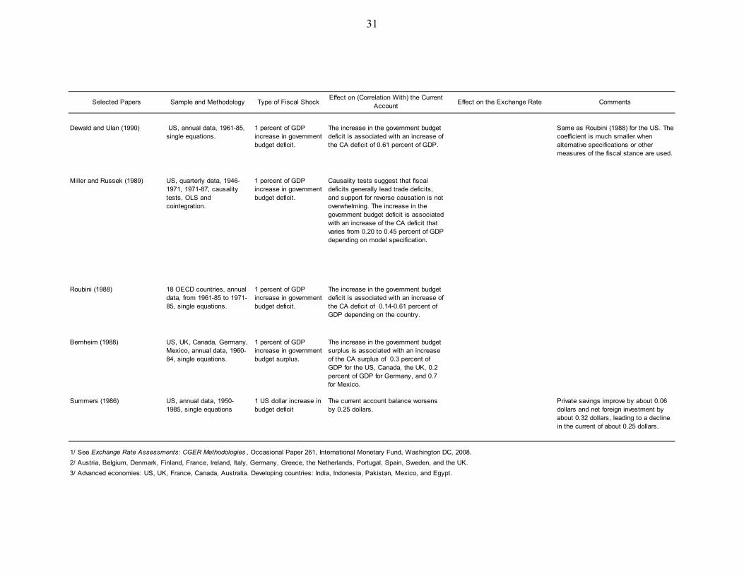
31

Selected Papers Sample and Methodology Type of Fiscal ShockEffect on (Correlation With) the Current

AccountEffect on the Exchange Rate Comments

Dewald and Ulan (1990) US, annual data, 1961-85, single equations.

1 percent of GDP increase in government budget deficit.

The increase in the government budget deficit is associated with an increase of the CA deficit of 0.61 percent of GDP.

Same as Roubini (1988) for the US. The coefficient is much smaller when alternative specifications or other measures of the fiscal stance are used.

Miller and Russek (1989) US, quarterly data, 1946-1971, 1971-87, causality tests, OLS and cointegration.

1 percent of GDP increase in government budget deficit.

Causality tests suggest that fiscal deficits generally lead trade deficits, and support for reverse causation is not overwhelming. The increase in the government budget deficit is associated with an increase of the CA deficit that varies from 0.20 to 0.45 percent of GDP depending on model specification.

Roubini (1988) 18 OECD countries, annual data, from 1961-85 to 1971-85, single equations.

1 percent of GDP increase in government budget deficit.

The increase in the government budget deficit is associated with an increase of the CA deficit of 0.14-0.61 percent of GDP depending on the country.

Bernheim (1988) US, UK, Canada, Germany, Mexico, annual data, 1960-84, single equations.

1 percent of GDP increase in government budget surplus.

The increase in the government budget surplus is associated with an increase of the CA surplus of 0.3 percent of GDP for the US, Canada, the UK, 0.2 percent of GDP for Germany, and 0.7 for Mexico.

Summers (1986) US, annual data, 1950-1985, single equations

1 US dollar increase in budget deficit

The current account balance worsens by 0.25 dollars.

Private savings improve by about 0.06 dollars and net foreign investment by about 0.32 dollars, leading to a decline in the current of about 0.25 dollars.

1/ See Exchange Rate Assessments: CGER Methodologies , Occasional Paper 261, International Monetary Fund, Washington DC, 2008.

2/ Austria, Belgium, Denmark, Finland, France, Ireland, Italy, Germany, Greece, the Netherlands, Portugal, Spain, Sweden, and the UK.

3/ Advanced economies: US, UK, France, Canada, Australia. Developing countries: India, Indonesia, Pakistan, Mexico, and Egypt.

32

Advanced Economies

Belgium 1999 (2, 4.5)

Czech Republic 1993 (3, 7.9)

Denmark 2005 (2, 3.3)

Estonia 1993 (1, 8.2) 2005 (2, 7.9) 1995 (2, 6.9) 2001 (3, 6.6)

Finland 1978 (2, 4.5) 2004 (1, 4.3) 2002 (1, 3.7)

Germany 1989 (2, 6) 1978 (2, 3.3)

Greece 1981 (2, 23.7) 2004 (3, 8.3) 1997 (3, 5.4) 1987 (3, 5.3) 1984 (1, 4)

Hong Kong SAR 1999 (1, 2.1)

Iceland 2002 (4, 26.9) 1997 (1, 5) 1994 (2, 3.7) 1999 (1, 3.5)

Ireland 1975 (4, 10.4) 1980 (1, 2.8)

Israel 1986 (1, 7.8) 1980 (2, 4.6) 2006 (1, 2.9)

Italy 1972 (2, 9.1) 1978 (3, 6.8)

Korea 1977 (3, 12.2) 1998 (4, 10.6) 1988 (3, 10.5) 2004 (2, 3.5)

Netherlands 1997 (1, 3.3)

New Zealand 1988 (1, 2.9) 1998 (1, 2.3)

Portugal 1980 (1, 11.7) 1995 (5, 10.1) 1986 (2, 5.3) 1993 (1, 2.6)

Singapore 1998 (2, 10.6) 2003 (1, 6.5) 1992 (1, 4.7) 1979 (1, 4.5) 1986 (1, 2.6) 1995 (1, 2.1)

Slovak Republic 1994 (2, 14.3) 2000 (1, 5)

Slovenia 2002 (2, 3.7)

Spain 1973 (1, 4)

Sweden 1978 (2, 3.1)

Switzerland 2000 (1, 4.4)

Emerging and Low-Income Countries

Afghanistan, I.R. of 2002 (1, 12)

Argentina 2002 (3, 6.8)

Benin 1994 (1, 3.4) 1996 (1, 3.2)

Bulgaria 2002 (5, 18)

Burkina Faso 1994 (3, 7.1) 1998 (2, 5.4) 1984 (1, 5.2)

Burundi 2005 (2, 15) 1997 (1, 6.7) 2002 (2, 5.9) 1995 (1, 5.5) 1999 (1, 3.5) 1991 (1, 3.2)

Cape Verde 1997 (2, 7.4) 2005 (2, 5.9) 2003 (1, 3)

Central African Rep. 2004 (1, 5.8)

Chile 1983 (1, 5.3) 1991 (2, 5)

China,P.R.: Mainland 1991 (2, 5.1)

Colombia 1991 (4, 8.7)

Congo, Dem. Rep. of 2003 (2, 11) 1996 (2, 8.4)

Côte d'Ivoire 2002 (3, 6.4) 2006 (1, 3.5)

Djibouti 2003 (4, 27) 1991 (1, 6.3) 1999 (1, 5.2)

Ethiopia 1998 (1, 5.4) 1995 (2, 4.5)

Gambia, The 2004 (1, 10) 1994 (2, 9.7) 1992 (1, 5.2)

Ghana 1995 (2, 12) 2003 (4, 12) 1998 (1, 6.7)

Hungary 1991 (2, 12) 1984 (2, 5.9)

Kyrgyz Republic 1997 (1, 13) 1994 (2, 12) 2004 (2, 8.1)

Lao People's Dem.Rep 2002 (3, 10) 2006 (1, 6.7) 1999 (1, 6.2)

Latvia 1994 (4, 14) 2005 (2, 10) 2002 (2, 6)

Liberia 2002 (1, 21) 2004 (2, 13) 2000 (1, 6.1)

Lithuania 2005 (2, 6.6)

Malawi 1993 (1, 15) 1990 (2, 8.7) 1998 (1, 7.8) 1988 (1, 7.7) 2000 (2, 7.1) 1984 (1, 6.1) 2003 (2, 4.3) 1996 (1, 3.8)

Malaysia 1987 (4, 16) 1999 (2, 7.8)

Maldives 2003 (1, 12) 1998 (1, 9.8) 1992 (1, 8.4) 1996 (1, 3.6)

Mali 2006 (1, 4.4)

Mauritania 2002 (3, 49) 2006 (1, 9.8)

Moldova 2004 (3, 14) 1995 (3, 13)

Mozambique 2006 (2, 16) 1985 (2, 11) 1997 (2, 8.4) 1990 (3, 7.1) 1988 (1, 3.7)

Pakistan 2003 (4, 9.6) 1973 (1, 8.6) 1992 (1, 3.5)

Philippines 2006 (2, 10) 2001 (1, 6.2) 1998 (1, 6) 1988 (2, 5) 1986 (1, 4.5) 1992 (1, 3.6)

Romania 2002 (5, 10) 1994 (2, 4.9) 1991 (1, 3.4)

Rwanda 1995 (2, 6.7) 2001 (2, 6.4) 2005 (1, 6)

São Tomé & Príncipe 1979 (3, 37) 2005 (1, 32) 1987 (2, 21) 1994 (1, 14) 1983 (1, 12) 2000 (1, 12) 2003 (1, 8.1) 1990 (2, 5) 1997 (1, 3.1)

Sierra Leone 1998 (2, 13) 1984 (6, 13) 1991 (2, 7.7) 1994 (2, 6.2)

St. Vincent & Grens. 2002 (2, 13) 2005 (2, 4.5)

Tajikistan 2005 (2, 8.4)

Tanzania 1996 (2, 7.7)

Thailand 1998 (7, 17) 1986 (4, 8.9) 1982 (1, 4.4)

Togo 1999 (1, 6) 1984 (2, 5) 1995 (2, 4.4)

Turkey 1998 (2, 4.5)

Uganda 1994 (2, 6.4) 1997 (2, 5.4) 1990 (1, 5) 1992 (1, 3.6)

Ukraine 2004 (3, 14)

Zambia 1980 (1, 6.5) 1983 (3, 6.2) 1988 (1, 4.2) 1991 (1, 3.9)

Appendix II – Listing of Large Episodes of Current Account and Fiscal Policy Changes Start years, followed by duration of episode and size of change in parenthesis

A. Current Account Deteriorations

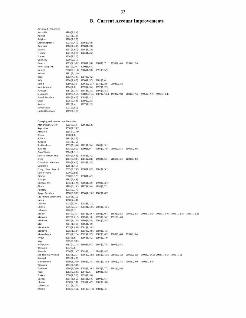
33

Advanced Economies

Australia 1999 (2, 3.4)

Austria 2001 (1, 3.5)

Belgium 1998 (1, 2.7)

Czech Republic 2003 (2, 4.7) 1996 (2, 4.5)

Denmark 1986 (2, 4.2) 1998 (1, 2.8)

Estonia 1997 (2, 6.7) 1994 (1, 2.8)

Finland 1991 (4, 9.4) 1983 (1, 2.2)

France 1974 (1, 2.1)

Germany 2000 (2, 3.7)

Greece 1985 (2, 10.2) 1978 (1, 9.6) 1980 (1, 7) 1990 (2, 4.6) 1993 (1, 2.4)

Hong Kong SAR 1997 (2, 10.7) 2000 (3, 6.3)

Iceland 2000 (2, 11.8) 2006 (1, 9.8) 1991 (3, 5.9)

Ireland 1981 (7, 12.9)

Israel 1982 (4, 12.3) 1987 (2, 4.2)

Italy 1974 (1, 6.7) 1976 (2, 5.5) 1981 (2, 4)

Korea 1980 (8, 16) 1996 (2, 15.7) 1975 (2, 8.5) 2002 (2, 3.2)

New Zealand 1984 (4, 8) 1999 (2, 3.4) 1997 (1, 2.5)

Portugal 1981 (5, 18.3) 1988 (1, 2.3) 1994 (1, 2.2)

Singapore 1980 (6, 15.5) 2000 (3, 11.6) 1987 (2, 10.4) 1993 (2, 9.8) 2004 (3, 7.6) 1996 (2, 7.2) 1990 (2, 3.4)

Slovak Republic 1998 (2, 6.3) 2005 (2, 3.1)

Spain 1976 (2, 4.9) 1969 (2, 3.3)

Sweden 1982 (2, 4) 1977 (1, 2.2)

Switzerland 2001 (6, 9.1)

United Kingdom 1989 (2, 3.3)

Emerging and Low-Income Countries

Afghanistan, I.R. of 2003 (2, 13) 2006 (1, 5.8)

Argentina 1998 (4, 13.7)

Armenia 1998 (4, 15.9)

Benin 1988 (1, 6)

Bolivia 1993 (1, 3.3)

Bulgaria 2001 (1, 3.2)

Burkina Faso 2005 (3, 14.8) 1982 (2, 5.4) 1988 (1, 3.1)

Burundi 1992 (3, 9.3) 1990 (1, 9) 2004 (1, 7.8) 2000 (2, 5.3) 1996 (1, 4.6)

Cape Verde 2004 (1, 11.1)

Central African Rep. 1998 (2, 4.8) 2005 (1, 3.2)

Chile 1984 (5, 10.1) 1981 (2, 8.8) 1998 (1, 5.1) 2005 (1, 3.4) 2003 (1, 3.2)

China,P.R.: Mainland 1989 (2, 4.2) 1993 (1, 3.3)

Colombia 1985 (1, 4.7)

Congo, Dem. Rep. of 2005 (3, 13.5) 1998 (1, 6.5) 2001 (2, 5.1)

Côte d'Ivoire 2000 (2, 9.5)

Djibouti 2000 (3, 12.1) 1998 (1, 4.1)

Ethiopia 1993 (2, 4.6)

Gambia, The 1996 (1, 12.5) 2005 (1, 3.5) 1990 (1, 3.4)

Ghana 1999 (4, 13.3) 1997 (1, 9.4) 1993 (2, 7.1)

Hungary 1993 (2, 7.4)

Kyrgyz Republic 1998 (3, 20.2) 1996 (1, 15.2) 2002 (2, 8.7)

Lao People's Dem.Rep 2005 (1, 7.2)

Latvia 1998 (2, 4.8)

Lesotho 2005 (2, 20.1) 2003 (1, 7.2)

Liberia 2006 (2, 36.7) 2003 (1, 12.6) 2001 (1, 10.1)

Lithuania 1998 (3, 7)

Malawi 1994 (2, 16.7) 1997 (1, 10.7) 1980 (1, 9.7) 1983 (1, 8.2) 2005 (2, 8.2) 2002 (1, 6.6) 1989 (1, 5.7) 1992 (1, 3.5) 1999 (1, 3.3)

Malaysia 1997 (2, 21.5) 1985 (2, 10.1) 1995 (1, 5.2) 1991 (1, 4.8)

Maldives 1993 (1, 12.8) 1999 (1, 5.5) 2001 (2, 5.3)

Mali 2001 (1, 7.3) 2005 (1, 4.5)

Mauritania 2005 (1, 45.8) 2001 (1, 14.2)

Moldova 1998 (1, 13.4) 1993 (2, 10.6) 2003 (1, 4.3)

Mozambique 1993 (4, 12.4) 2002 (2, 9.9) 1982 (3, 6.9) 1989 (1, 4.8) 1999 (1, 3.4)

Nepal 1998 (1, 5) 1996 (1, 4.2) 1994 (1, 3.9)

Niger 2005 (3, 10.3)

Philippines 1982 (4, 11.8) 1999 (2, 9.7) 1997 (1, 7.5) 1990 (2, 4.2)

Romania 1992 (2, 6)

Rwanda 2006 (2, 13.7) 2003 (2, 11.1) 1993 (2, 8.5)

São Tomé & Príncipe 1982 (1, 25) 1995 (2, 18.8) 1985 (1, 16.6) 2006 (1, 15) 2001 (2, 15) 1992 (2, 14.6) 2004 (1, 9.1) 1989 (1, 5)

Senegal 1993 (1, 4.2)

Sierra Leone 1990 (1, 16.9) 1996 (2, 15.1) 1981 (3, 10.8) 2000 (2, 7.2) 2005 (1, 3.9) 1993 (1, 3.4)

Tanzania 1994 (2, 10.5)

Thailand 1996 (2, 20.6) 2005 (2, 10.7) 1983 (3, 7.7) 1981 (1, 4.6)

Togo 1982 (2, 12.1) 1997 (2, 6) 1990 (1, 3.3)

Turkey 2000 (1, 5.7) 1993 (1, 3.6)

Uganda 1993 (1, 8.2) 1991 (1, 5.8) 1999 (2, 5.7)

Ukraine 1998 (2, 7.8) 2003 (1, 4.9) 2001 (1, 3.8)

Uzbekistan 2002 (5, 17.8)

Zambia 1986 (2, 16.6) 1981 (2, 11.8) 1989 (2, 4.1)

B. Current Account Improvements

34

Advanced Economies

Austria 1977 (2, 16.7) 1983 (4, 6.3) 2003 (1, 3.2)

Belgium 1979 (2, 4.3) 2003 (2, 3.9)

Canada 1974 (3, 7.2)

Czech Republic 1993 (2, 19.2)

Denmark 1973 (3, 5)

Estonia 1994 (2, 4) 1997 (2, 4)

Finland 1989 (4, 8.6) 1976 (4, 6.7) 1981 (2, 3.7) 1986 (1, 2.4)

Germany 2000 (2, 4.6) 1989 (2, 4.5)

Greece 1988 (1, 3.3)

Hong Kong SAR 1997 (1, 6.9) 1999 (2, 6.2) 1980 (3, 4.9)

Iceland 1984 (2, 6.4) 1992 (2, 3.5) 1973 (1, 3.5) 2000 (2, 3.5) 1976 (1, 2.4) 1978 (1, 2.3) 1982 (1, 2)

Ireland 2000 (2, 5) 1976 (2, 4.7)

Israel 1986 (4, 11.8) 1994 (2, 4.9) 1983 (1, 4.6) 1991 (1, 2.6)

Japan 1974 (2, 3.5) 1977 (1, 2.2)

Korea 1976 (2, 6.3)

Netherlands 1988 (2, 3.2)

Portugal 1985 (2, 3.8) 2003 (2, 3.7) 1992 (1, 2.3)

Singapore 1993 (5, 9.9)

Slovak Republic 1994 (3, 7.4) 1999 (1, 3.3)

Spain 1981 (1, 3.1)

Sweden 1987 (6, 14.3)

United Kingdom 1989 (4, 7.2) 2006 (2, 3.5)

United States 2000 (3, 6.1) 1974 (1, 3.5)

Emerging and Low-Income Countries

Bolivia 1986 (1, 6.3)

Bulgaria 2000 (2, 4.8)

Burkina Faso 2006 (1, 22.3) 1989 (2, 6) 1992 (1, 4.9)

Burundi 1995 (1, 4.2) 2002 (1, 3.3)

Cape Verde 1998 (2, 18.4) 1990 (4, 11.2)

Central African Rep. 1993 (1, 16.9) 1997 (1, 9.4) 1987 (1, 5.4) 1995 (1, 3.8)

Comoros 1993 (2, 8.6) 1997 (1, 4.3)

Djibouti 1980 (3, 16.4) 1991 (1, 9.4) 1989 (1, 6.7) 1985 (1, 5.3) 1998 (1, 3.4)

Dominica 1988 (2, 13.7) 1996 (3, 8.2) 1992 (2, 4.7)

Ethiopia 1997 (3, 6.8)

Gambia, The 2000 (1, 15.1) 1992 (3, 10.6) 1982 (1, 4.8) 1988 (1, 4.4)

Georgia 2004 (3, 14.1)

Guinea-Bissau 1994 (3, 22.2) 1980 (1, 20.2) 1986 (2, 14.9) 1990 (2, 13.7) 1983 (1, 4.9)

Guyana 1993 (5, 16) 1999 (4, 10.1)

Hungary 1999 (3, 8.4) 1990 (3, 7.2) 2004 (2, 4.4)

Kyrgyz Republic 1994 (1, 4)

Latvia 1993 (1, 5.5)

Lesotho 1993 (6, 18.8) 1984 (3, 11.8) 1981 (1, 3.3) 2001 (1, 3.3)

Lithuania 1997 (2, 4.7)

Madagascar 2006 (1, 40.7) 1997 (1, 4.2) 1988 (1, 3.9) 1990 (1, 3.2)

Malawi 1989 (3, 9.8) 2006 (1, 6.2) 1993 (1, 3.8)

Malaysia 1997 (3, 8.2)

Maldives 1990 (2, 25.8) 1979 (1, 15.2) 2004 (3, 7.5) 1982 (1, 6.2) 1988 (1, 5.9)

Mali 2006 (1, 34.4)

Mauritania 2006 (1, 36.8) 2002 (1, 8.9)

Moldova 1995 (2, 8) 2001 (1, 4.2)

Mongolia 2006 (1, 6.1) 1997 (1, 5.7)

Mozambique 1982 (1, 8.6) 1980 (1, 7.1) 2000 (2, 5.4) 1992 (2, 5.1)

Myanmar 1999 (1, 3.9)

Nicaragua 1995 (1, 6.7) 1993 (1, 5.6)

Niger 2006 (1, 40.8) 1980 (1, 4.1)

Poland 1988 (1, 9.6) 1985 (2, 5.5)

Romania 1993 (3, 7.9) 1989 (1, 7.2) 1991 (1, 5.7)

Rwanda 1995 (1, 6)

São Tomé & Príncipe 2005 (1, 50.2) 1981 (1, 16.9) 1997 (3, 13) 1988 (1, 9) 1983 (1, 6.8) 2002 (2, 6) 1993 (1, 3.8) 1986 (1, 3.6)

Senegal 2002 (2, 4.5) 1991 (2, 4) 2000 (1, 3.9)

Sierra Leone 1992 (3, 7.6) 1988 (2, 4.4) 2000 (2, 4.4)

St. Lucia 1998 (1, 5.7) 1985 (1, 3.4)

Tajikistan 2006 (1, 8.2) 1995 (1, 7.2)

Tanzania 1990 (3, 7)

Togo 1984 (3, 6.8) 2003 (3, 6.4) 1992 (1, 5.1)

Turkey 1990 (1, 3.8)

Uganda 1998 (2, 8.7)

Ukraine 2002 (2, 7.1) 1996 (1, 3.3)

Uzbekistan 1992 (1, 17.6) 1995 (1, 4.4)

Zambia 2006 (1, 21.4) 1987 (2, 9.9) 1981 (1, 9.6) 1995 (3, 7.6) 1984 (1, 6.4) 1999 (2, 4.3)

Ukraine 2002 (2, 7.1) 1996 (1, 3.3)

Uzbekistan 1992 (1, 17.6) 1995 (1, 4.4)

Zambia 2006 (1, 21.4) 1987 (2, 9.9) 1981 (1, 9.6) 1995 (3, 7.6) 1984 (1, 6.4) 1999 (2, 4.3)

C. Cyclically-Adjusted Primary Balance Deteriorations

35

Advanced Economies

Austria 1982 (1, 6.1) 1995 (2, 4.5) 1976 (1, 4.5) 2000 (1, 2.7) 2004 (1, 2.5)

Belgium 1983 (4, 7.3) 1981 (1, 4.7) 2005 (1, 2.2)

Canada 1992 (5, 8) 1985 (2, 4.3)

Czech Republic 1995 (2, 10.2) 2002 (2, 3.9)

Denmark 1982 (4, 12.3)

Finland 1995 (5, 12.2) 1980 (1, 2.5) 1983 (1, 2.2)

Germany 1988 (1, 2)

Greece 1989 (6, 12.1) 2004 (2, 4)

Hong Kong SAR 2001 (6, 12) 1995 (2, 6.1) 1990 (1, 2.6) 1998 (1, 2.4)

Iceland 1974 (2, 6.3) 2002 (4, 6.3) 1994 (3, 4.8) 1983 (1, 4.2)

Ireland 1978 (6, 11.6) 1986 (3, 9.5)

Israel 1984 (2, 16.9) 1980 (3, 11.1)

Italy 1990 (3, 5.3)

Korea 1999 (1, 2.5)

Netherlands 1990 (1, 3) 1992 (1, 2.5)

Portugal 1983 (2, 6.1) 1993 (2, 3.6) 1987 (1, 3.6) 1981 (1, 2.3) 1991 (1, 2.2)

Slovak Republic 1992 (2, 10.6) 1997 (2, 3.4)

Spain 1995 (2, 3.2)

Sweden 1993 (5, 12.2) 1982 (5, 9.4) 1980 (1, 3.2)

Emerging and Low-Income Countries

Argentina 2001 (3, 7)

Armenia 1994 (1, 8)

Bolivia 2002 (4, 12) 1985 (1, 7.4) 1993 (2, 4.5)

Brazil 1997 (2, 4.9) 1991 (1, 3.1)

Bulgaria 1993 (1, 7.8)

Burkina Faso 2005 (1, 21.6) 1988 (1, 7.6)

Burundi 1999 (1, 5.1) 1996 (1, 3.9) 2001 (1, 3.1)

Cape Verde 2000 (1, 13.3) 1994 (4, 13.2) 1986 (2, 6.4) 2002 (2, 5) 2006 (1, 3.7)

Central African Rep. 1990 (3, 14.2) 1994 (1, 10.8) 1998 (1, 7.2) 1996 (1, 6.2) 2000 (2, 4.1) 1988 (1, 3.3)

Comoros 1998 (1, 6.4) 1995 (2, 5.1) 1992 (1, 5) 1988 (1, 3)

Djibouti 1992 (4, 9.7) 1990 (1, 5.5) 1983 (2, 5.4) 1986 (1, 5.3) 1997 (1, 4.5) 1988 (1, 3.9)

Dominica 1999 (4, 13.1) 1990 (2, 8.8) 1994 (2, 4.7)

Ethiopia 2002 (2, 5.6) 1990 (2, 4.7) 2000 (1, 3.8)

Gambia, The 2001 (2, 12) 1985 (1, 8.2) 1995 (3, 7.9) 1987 (1, 6.9) 2006 (1, 5.8) 1983 (1, 4.7) 1999 (1, 3.5)

Georgia 1994 (1, 11.9) 2003 (1, 5.6)

Guinea 2003 (2, 5.6)

Guinea-Bissau 1992 (2, 20.7) 1997 (2, 15.3) 1981 (2, 12.4) 1984 (2, 11.9) 1988 (2, 6.9)

Guyana 1998 (1, 3.9)

Hungary 1993 (3, 9.3) 2006 (1, 4.7)

Kyrgyz Republic 1999 (3, 7.4) 1993 (1, 6.9) 1995 (1, 4.9)

Lao People's Dem.Rep 1998 (1, 3.5) 2003 (1, 3.1)

Latvia 1992 (1, 4.9)

Lesotho 1987 (6, 22.7) 2002 (5, 17.5) 1999 (2, 13.7) 1982 (2, 8.9) 1980 (1, 3.9)

Lithuania 1999 (3, 6.9)

Madagascar 2004 (2, 42.3) 1980 (8, 16.4) 1989 (1, 3.2)

Malawi 1980 (5, 12.2) 1994 (1, 9.9) 2001 (2, 7.6) 1987 (2, 5.8)

Maldives 1989 (1, 18.4) 1980 (2, 17.8) 1992 (2, 7) 1986 (2, 6.9) 1983 (1, 5.3)

Mali 2005 (1, 34.1) 1999 (1, 3.2)

Mauritania 2005 (1, 39.9) 2001 (1, 8.1) 2003 (1, 7.1) 1995 (1, 4)

Moldova 1992 (3, 28.9) 1997 (4, 11.4)

Mongolia 2002 (4, 11.3) 1998 (3, 9.2)

Mozambique 1986 (3, 6) 1990 (2, 5.7) 1983 (2, 5.3) 1981 (1, 4.3) 2002 (1, 3.8) 1994 (1, 3.7)

Myanmar 2000 (2, 4.7)

Nicaragua 1991 (2, 7.9) 1994 (1, 6.4) 2001 (1, 6.1)

Niger 2004 (2, 42.9) 1981 (3, 9.1) 1994 (2, 6.3) 1999 (1, 3.1)

Poland 1989 (1, 11.2)

Romania 1996 (3, 8.4) 1990 (1, 5.2) 1983 (1, 3.5)

Rwanda 1992 (3, 14.8) 1999 (1, 5.3)

São Tomé & Príncipe 2004 (1, 53.1) 1980 (1, 14.7) 2000 (2, 13) 1982 (1, 11.5) 1984 (2, 10.6) 1992 (1, 6.3)

Senegal 2001 (1, 4)

Sierra Leone 2002 (5, 32.5) 1990 (2, 6.5) 1998 (2, 4.3) 1995 (1, 3.9)

St. Lucia 1996 (2, 5.6) 1986 (1, 5.2) 1983 (2, 5.2) 2002 (1, 4.2)

Tajikistan 2005 (1, 6.2) 1996 (1, 4.6)

Togo 2000 (1, 4.9) 1993 (2, 4.7) 1996 (1, 3.1)

Turkey 1987 (3, 12.4) 1997 (4, 8.6) 1993 (1, 5)

Uganda 2000 (1, 6.9)

Ukraine 1994 (2, 5.6)

Uzbekistan 1993 (2, 13) 1996 (1, 5.8)

Zambia 2005 (1, 21.6) 1982 (2, 14.4) 1989 (4, 10.6) 1985 (2, 7.3) 1977 (1, 6.8) 1979 (2, 5.8) 2001 (1, 4)

D. Cyclically-Adjusted Primary Balance Improvements

36

Appendix III – Event Study of Large Changes in External and CAPB Balances in Advanced Economies

Current account Cyclically-adjusted Primary Balance Increases Declines Increases Declines

-10

-5

0

5

10

15

-3 -2 -1 0 1 2 3 4

Current Account

std mean std -

-8

-6

-4

-2

0

2

4

6

8

-3 -2 -1 0 1 2 3 4

Fiscal Balance

std mean std -

-8

-6

-4

-2

0

2

4

6

-3 -2 -1 0 1 2 3 4

SPB

std mean std -

-8

-6

-4

-2

0

2

4

6

8

-3 -2 -1 0 1 2 3 4

GSIB

std mean std -

-8

-6

-4

-2

0

2

4

6

8

-3 -2 -1 0 1 2 3 4

GS

std mean std -

-3

-2

-1

0

1

2

3

4

-3 -2 -1 0 1 2 3 4

GI

std mean std -

-10

-5

0

5

10

15

-3 -2 -1 0 1 2 3 4

PSIB

std mean std -

-10

-8

-6

-4

-2

0

2

4

6

8

10

12

-3 -2 -1 0 1 2 3 4

PS

std mean std -

-10

-8

-6

-4

-2

0

2

4

6

-3 -2 -1 0 1 2 3 4

PI

std mean std -

-15

-10

-5

0

5

10

-3 -2 -1 0 1 2 3 4

Current Account

std mean std -

-8

-6

-4

-2

0

2

4

6

8

-3 -2 -1 0 1 2 3 4

Fiscal Balance

std mean std -

-8

-6

-4

-2

0

2

4

6

-3 -2 -1 0 1 2 3 4

SPB

std mean std -

-8

-6

-4

-2

0

2

4

6

8

-3 -2 -1 0 1 2 3 4

GSIB

std mean std -

-8

-6

-4

-2

0

2

4

6

8

-3 -2 -1 0 1 2 3 4

GS

std mean std -

-3

-2

-1

0

1

2

3

-3 -2 -1 0 1 2 3 4

GI

std mean std -

-15

-10

-5

0

5

10

-3 -2 -1 0 1 2 3 4

PSIB

std mean std -

-12

-10

-8

-6

-4

-2

0

2

4

6

8

-3 -2 -1 0 1 2 3 4

PS

std mean std -

-6

-4

-2

0

2

4

6

8

10

-3 -2 -1 0 1 2 3 4

PI

std mean std -

-8

-6

-4

-2

0

2

4

6

8

-3 -2 -1 0 1 2 3 4

Current Account

std mean std -

-6

-4

-2

0

2

4

6

8

10

-3 -2 -1 0 1 2 3 4

Fiscal Balance

std mean std -

-6

-4

-2

0

2

4

6

8

10

-3 -2 -1 0 1 2 3 4

SPB

std mean std -

-8

-6

-4

-2

0

2

4

6

8

10

-3 -2 -1 0 1 2 3 4

GSIB

std mean std -

-8

-6

-4

-2

0

2

4

6

8

10

-3 -2 -1 0 1 2 3 4

GS

std mean std -

-2

-1

-1

0

1

1

2

-3 -2 -1 0 1 2 3 4

GI

std mean std -

-12

-10

-8

-6

-4

-2

0

2

4

6

8

-3 -2 -1 0 1 2 3 4

PSIB

std mean std -

-10

-8

-6

-4

-2

0

2

4

6

-3 -2 -1 0 1 2 3 4

PS

std mean std -

-6

-4

-2

0

2

4

6

-3 -2 -1 0 1 2 3 4

PI

std mean std -

-6

-4

-2

0

2

4

6

-3 -2 -1 0 1 2 3 4

Current Account

std mean std -

-10

-8

-6

-4

-2

0

2

4

6

-3 -2 -1 0 1 2 3 4

Fiscal Balance

std mean std -

-10

-8

-6

-4

-2

0

2

4

6

-3 -2 -1 0 1 2 3 4

SPB

std mean std -

-8

-6

-4

-2

0

2

4

6

-3 -2 -1 0 1 2 3 4

GSIB

std mean std -

-8

-6

-4

-2

0

2

4

6

-3 -2 -1 0 1 2 3 4

GS

std

-2

-1

-1

0

1

1

2

2

-3 -2 -1 0 1 2 3 4

GI

std mean std -

-8

-6

-4

-2

0

2

4

6

8

10

-3 -2 -1 0 1 2 3 4

PSIB

std mean std -

-8

-6

-4

-2

0

2

4

6

8

-3 -2 -1 0 1 2 3 4

PS

std mean std -

-6

-4

-2

0

2

4

6

-3 -2 -1 0 1 2 3 4

PI

std mean std -

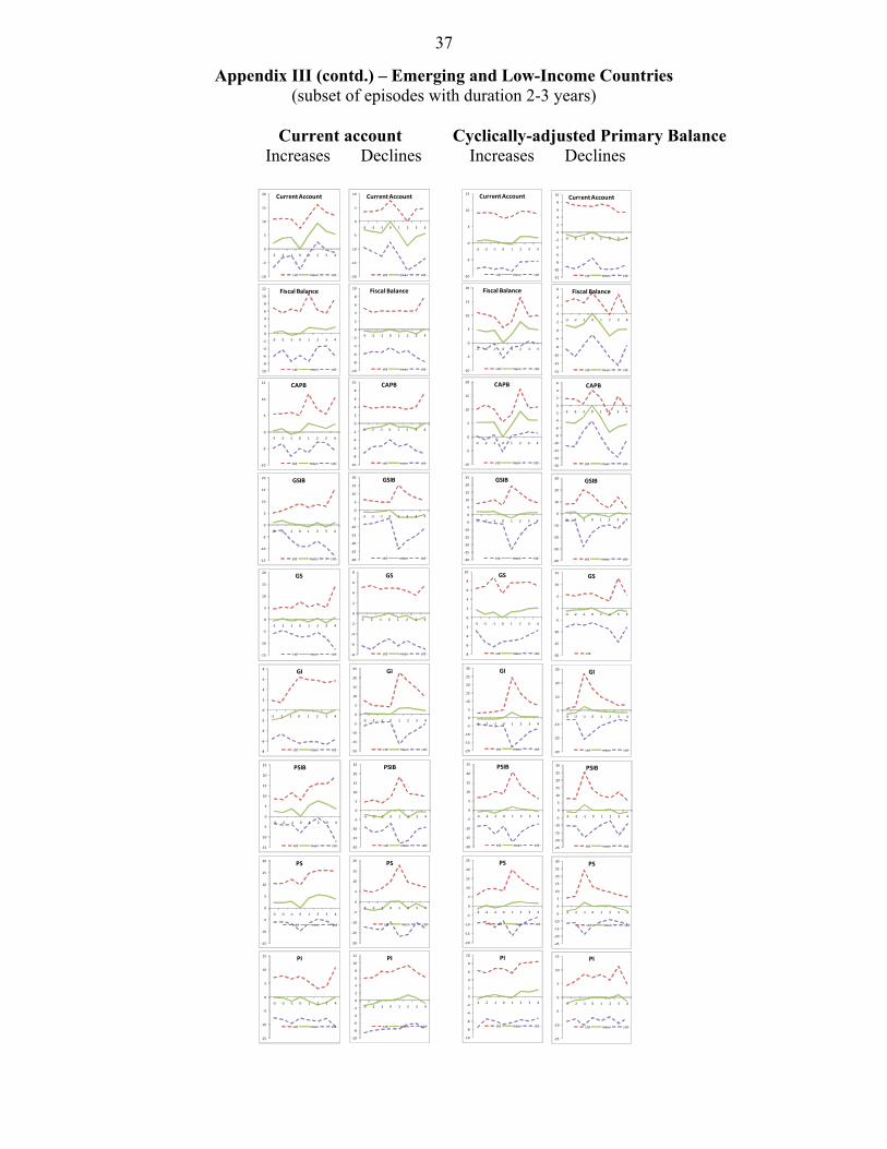
37

Appendix III (contd.) – Emerging and Low-Income Countries (subset of episodes with duration 2-3 years)

Current account Cyclically-adjusted Primary Balance Increases Declines Increases Declines

-10

-5

0

5

10

15

20

-3 -2 -1 0 1 2 3 4

Current Account

std mean std -

-10

-8

-6

-4

-2

0

2

4

6

8

10

12

-3 -2 -1 0 1 2 3 4

Fiscal Balance

std mean std -

-10

-5

0

5

10

15

-3 -2 -1 0 1 2 3 4

CAPB

std mean std -

-15

-10

-5

0

5

10

15

20

-3 -2 -1 0 1 2 3 4

GSIB

std mean std -

-15

-10

-5

0

5

10

15

20

-3 -2 -1 0 1 2 3 4

GS

std mean std -

-8

-6

-4

-2

0

2

4

6

8

-3 -2 -1 0 1 2 3 4

GI

std mean std -

-15

-10

-5

0

5

10

15

20

25

-3 -2 -1 0 1 2 3 4

PSIB

std mean std -

-15

-10

-5

0

5

10

15

20

-3 -2 -1 0 1 2 3 4

PS

std mean std -

-15

-10

-5

0

5

10

15

-3 -2 -1 0 1 2 3 4

PI

std mean std -

-20

-15

-10

-5

0

5

10

-3 -2 -1 0 1 2 3 4

Current Account

std mean std -

-10

-8

-6

-4

-2

0

2

4

6

8

10

-3 -2 -1 0 1 2 3 4

Fiscal Balance

std mean std -

-10

-8

-6

-4

-2

0

2

4

6

8

10

-3 -2 -1 0 1 2 3 4

CAPB

std mean std -

-30

-25

-20

-15

-10

-5

0

5

10

15

20

-3 -2 -1 0 1 2 3 4

GSIB

std mean std -

-8

-6

-4

-2

0

2

4

6

8

-3 -2 -1 0 1 2 3 4

GS

std mean std -

-20

-15

-10

-5

0

5

10

15

20

25

-3 -2 -1 0 1 2 3 4

GI

std mean std -

-20

-15

-10

-5

0

5

10

15

20

25

-3 -2 -1 0 1 2 3 4

PSIB

std mean std -

-20

-15

-10

-5

0

5

10

15

20

-3 -2 -1 0 1 2 3 4

PS

std mean std -

-10

-8

-6

-4

-2

0

2

4

6

8

10

12

-3 -2 -1 0 1 2 3 4

PI

std mean std -

-10

-5

0

5

10

15

-3 -2 -1 0 1 2 3 4

Current Account

std mean std -

-10

-5

0

5

10

15

20

-3 -2 -1 0 1 2 3 4

Fiscal Balance

std mean std -

-10

-5

0

5

10

15

20

-3 -2 -1 0 1 2 3 4

CAPB

std mean std -

-30

-25

-20

-15

-10

-5

0

5

10

15

20

25

-3 -2 -1 0 1 2 3 4

GSIB

std mean std -

-8

-6

-4

-2

0

2

4

6

8

10

-3 -2 -1 0 1 2 3 4

GS

std mean std -

-20

-15

-10

-5

0

5

10

15

20

25

30

-3 -2 -1 0 1 2 3 4

GI

std mean std -

-20

-15

-10

-5

0

5

10

15

20

25

-3 -2 -1 0 1 2 3 4

PSIB

std mean std -

-20

-15

-10

-5

0

5

10

15

20

25

-3 -2 -1 0 1 2 3 4

PS

std mean std -

-10

-8

-6

-4

-2

0

2

4

6

8

10

-3 -2 -1 0 1 2 3 4

PI

std mean std -

-12

-10

-8

-6

-4

-2

0

2

4

6

8

10

-3 -2 -1 0 1 2 3 4

Current Account

std mean std -

-14

-12

-10

-8

-6

-4

-2

0

2

4

6

-3 -2 -1 0 1 2 3 4

Fiscal Balance

std mean std -

-16

-14

-12

-10

-8

-6

-4

-2

0

2

4

6

-3 -2 -1 0 1 2 3 4

CAPB

std mean std -

-40

-30

-20

-10

0

10

20

30

-3 -2 -1 0 1 2 3 4

GSIB

std mean std -

-20

-15

-10

-5

0

5

10

15

-3 -2 -1 0 1 2 3 4

GS

std

-30

-20

-10

0

10

20

30

-3 -2 -1 0 1 2 3 4

GI

std mean std -

-25

-20

-15

-10

-5

0

5

10

15

20

25

30

-3 -2 -1 0 1 2 3 4

PSIB

std mean std -

-25

-20

-15

-10

-5

0

5

10

15

20

25

30

-3 -2 -1 0 1 2 3 4

PS

std mean std -

-15

-10

-5

0

5

10

15

-3 -2 -1 0 1 2 3 4

PI

std mean std -

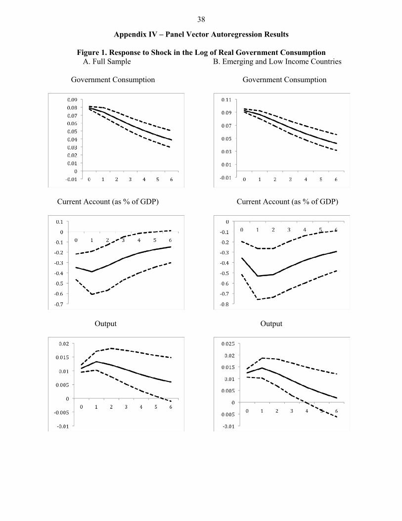
38

Appendix IV – Panel Vector Autoregression Results

Figure 1. Response to Shock in the Log of Real Government Consumption A. Full Sample B. Emerging and Low Income Countries Government Consumption Government Consumption

Current Account (as % of GDP) Current Account (as % of GDP)

Output Output

39

Figure 1. Response to Shock in the Log of Real Government Consumption (cont.)

C. More Open Economies D. Less Open Economies Government Consumption Government Consumption

Current Account (as % of GDP) Current Account (as % of GDP)

Output Output

40

Figure 2. Response to Shock in the Log of Real Government Consumption (4 variable VAR)

A. Full Sample B. Emerging and low-income countries

Government Consumption Government Consumption

Current Account (as % of GDP) Current Account (as % of GDP)

Real Exchange Rate Real Exchange Rate

Output Output

41

Figure 3. Response to Shock in the Log of Real Government Consumption Quarterly Data

A. Full Sample B. Emerging and Low Income Countries Government Consumption Government Consumption

Current Account (as % of GDP) Current Account (as % of GDP)

Output Gap Output Gap

42

Figure 3. Response to Shock in the Log of Real Government Consumption Quarterly Data (contd.)

C. More Open Economies D. Less Open Economies Government Consumption Government Consumption

Current Account (as % of GDP) Current Account (as % of GDP)

Output Gap Output Gap

43

Figure 4. Response of the Current Account to GDP ratio to a Shock in the Log of Real Government Consumption across different exchange rate regimes.

Quarterly Data

44

45

Appendix V – Panel Vector Autoregression Data Availability A. Annual Data

Country Start End Country Start EndAlbania 1990 2006 Czech Republic 1993 2006Algeria 1977 1991 Denmark 1975 2006Angola 1985 1998 Djibouti 1991 2006Antigua and Barb. 1977 2002 Dominica 1991 2005Argentina 1976 2006 Dom. Rep. 1968 2007Armenia 1993 2007 Ecuador 1976 2006Australia 1965 2006 Egypt 1977 2006Austria 1967 2006 El Salvador 1976 2006Bahamas, The 1977 1987 Eritrea 1992 2000Bahrain, Kingdom of 1980 1985 Estonia 1992 2006Bangladesh 1976 2006 Ethiopia 1981 2006Barbados 1991 2002 Fiji 1979 1995Belarus 1993 2007 Finland 1975 2006Belgium 1975 2006 France 1975 2006Belize 1984 2006 Gabon 1978 2004Benin 1974 2005 Gambia, The 1978 2004Bolivia 1976 2006 Georgia 1997 2007Bosnia & Herz. 2002 2007 Germany 1971 2006Botswana 1975 2006 Ghana 1975 2006Brazil 1975 2007 Greece 1976 2006Brunei Darussalam 2001 2006 Grenada 1977 1999Bulgaria 1980 2007 Guatemala 1977 2005Burkina Faso 1974 2001 Guinea 1986 2004Burundi 1985 1996 Guinea-Bissau 1982 2004Cambodia 1993 2006 Guyana 1977 2002Cameroon 1977 2004 Haiti 1971 1990Canada 1965 2005 Honduras 1974 2006Cape Verde 1986 2007 Hungary 1982 2006Chad 1977 1994 Iceland 1976 2006Chile 1975 2006 India 1975 2006China, Mainland 1982 2006 Indonesia 1981 2007China,Hong Kong 1998 2007 Iran, I.R. of 1976 2000Colombia 1968 2007 Ireland 1974 2005Comoros 1980 1995 Israel 1995 2006Congo, Republic of 1978 1996 Italy 1970 2006Costa Rica 1977 2007 Japan 1977 2005CÙte d'Ivoire 1975 2007 Jordan 1976 2006Croatia 1995 2007 Kazakhstan 1995 2007Cyprus 1976 1994 Korea 1976 2007

46

A. Annual Data (Cont.)

Country Start End Country Start EndKuwait 1995 2004 Rwanda 1976 2007Kyrgyz Republic 1993 2006 Saudi Arabia 1997 2003Lao PDR 2000 2001 Senegal 1974 2004Latvia 1992 2006 Seychelles 1984 2006Lebanon 2002 2007 Sierra Leone 1980 1995Lesotho 1975 2006 Singapore 2002 2005Libya 1977 1983 Slovak Republic 1993 2003Lithuania 1995 2006 Slovenia 1992 2007Luxembourg 1995 2006 Somalia 1977 1989Macedonia, FYR 1996 2006 South Africa 1961 2007Madagascar 1974 2005 Spain 1975 2006Malawi 1977 2002 Sri Lanka 1989 2002Malaysia 1974 2007 St. Kitts & Nev. 1980 2003Maldives 1995 2004 St. Vincent & G. 1978 2003Mali 1975 2006 Sudan 1977 2006Malta 1982 1993 Suriname 1990 1994Mauritania 1975 1992 Swaziland 1980 2006Mauritius 1980 2006 Sweden 1970 2006Mexico 1979 2006 Switzerland 1977 2005Moldova 1994 2007 Syria 1977 2006Morocco 1975 2006 Tajikistan 2002 2006Mozambique 1980 2006 Tanzania 1990 2006Namibia 1990 2006 Thailand 1975 2007Netherlands 1967 2006 Togo 1974 2005New Zealand 1972 2005 Trin.and Tobago 1975 2005Nicaragua 1977 2006 Tunisia 1976 2006Niger 1974 1999 Turkey 1998 2006Norway 1975 2006 Uganda 1982 2007Oman 1988 2004 Ukraine 1994 2007Pakistan 1976 2007 United Kingdom 1970 2006Panama 1980 2007 United States 1970 2005Papua New G. 1976 2005 Uruguay 1978 2007Paraguay 1989 2006 Vanuatu 1983 1995Peru 1977 2006 Venezuela 1974 2007Philippines 1977 2006 Vietnam 1996 2007Poland 1990 2007 Zambia 1978 2007Portugal 1975 2006 Zimbabwe 1977 1994Romania 1990 2007 Russia 1994 2007

47

B. Quarterly Data

Country Start End Country Start EndArgentina 1993q1 2010q3 Korea 1976q1 2010q3Australia 1970q1 2010q4 Latvia 1995q1 2010q4Austria 1988q1 2010q4 Lithuania 1995q1 2010q4Belgium 1980q1 2010q4 Luxembourg 1995q1 2010q3Brazil 1995q1 2010q3 Malaysia 1999q1 2006q4Bulgaria 1997q1 2010q4 Malta 2000q1 2010q4Canada 1970q1 2010q4 Netherlands 1988q1 2010q3Chile 1996q1 2010q3 New Zealand 1987q2 2010q4Colombia 1996q1 2007q4 Norway 1978q1 2010q4Croatia 2000q1 2010q3 Peru 1994q1 2010q2Cyprus 1995q1 2010q4 Philippines 1981q1 2010q1Czech Rep. 1996q1 2010q3 Poland 1995q1 2010q4Denmark 1990q1 2010q4 Portugal 1995q1 2010q3Estonia 1995q1 2010q3 Romania 2000q1 2010q4Finland 1975q1 2010q4 Russia 1995q1 2009q3France 1978q1 2010q4 Singapore 2003q1 2009q4Germany 1991q1 2010q4 Slovak Rep. 1997q1 2010q4Greece 2000q1 2010q3 Slovenia 1995q1 2010q4Hungary 1995q1 2010q4 South Africa 1970q1 2010q4Iceland 1997q1 2010q4 Spain 1995q1 2010q4India 2004q1 2009q3 Sweden 1993q1 2010q4Indonesia 1997q1 2010q4 Switzerland 1980q1 2010q3Ireland 1997q1 2010q4 Thailand 1993q1 2010q2Israel 1995q1 2010q3 Turkey 1998q1 2010q3Italy 1981q1 2010q4 U.K. 1970q1 2010q4Japan 1980q1 2010q4 United States 1970q1 2010q4