Fiscal Consolidation with Tax Evasion and Corruption

Evi Pappa∗ Rana Sajedi† Eugenia Vella‡

July 2, 2014

Abstract

Using cross country data we show that tax evasion and corruption are highly importantfor determining the size of the fiscal multiplier. We introduce these two features in a NewKeynesian model with search and matching frictions, in order to revisit the effects of tax andexpenditure based consolidations. VAR evidence for Italy suggests that expenditure basedconsolidations reduce tax evasion significantly, while tax based ones increase it. In the model,expenditure cuts reduce demand for both formal and informal goods, and, thus, tax evasion.Tax hikes induce agents to work and produce more in the informal sector, which is less pro-ductive, and so imply higher output and welfare losses. We use the model to assess the lossesfrom the recent fiscal consolidation plans in Italy, Spain, Portugal and Greece. Policy conclu-sions are sensitive to the model’s assumptions. Counterfactual exercises highlight the benefitof fighting tax evasion and corruption in economies undertaking fiscal consolidation.

JEL classification: E32, F41Keywords: DSGE model, matching frictions, shadow economy, corruption, fiscal consoli-

dation, VAR, policy analysis.

∗Corresponding author, European University Institute, e-mail: evi.pappa@eui.eu†European University Institute, e-mail: rana.sajedi@eui.eu‡Max Weber Programme, European University Institute, e-mail: eugenia.vella@eui.eu

1

1 Introduction

When there is an income tax, the just man will pay more and the unjust less on the same amount

of income. Plato, The Republic, Book I, 343-D

The recent fiscal crisis has excited renewed interest in research examining the macroeconomic

impacts of fiscal consolidations.1 Besides this increasing attention, two crucial aspects of political

economy, namely the presence of tax evasion and corruption, have been left unnoticed. This is

despite the fact that many countries undertaking such policies are characterized by high levels of

both.2 Tax evasion and corruption often coexist, in various forms, and possibly interact. Existing

evidence suggests a positive correlation between the two (Buehn and Schneider (2012)). At the

same time, there is growing evidence of a rise in tax evasion and corruption since the crisis. For

example, a recent report by the union of the technical staff of the Finance Ministry of Spain

(Gestha (2014)) calculates that the shadow economy has increased by 6.8 pp between 2008 and

2012, reaching 24.6% of GDP. Similarly, a Greek police special task force reported in 2013 that

the number of cases of public corruption increased by 33% between 2011 and 2012.3 The aim of

this paper is to consider these two features and to revisit the effects of expenditure based (EB)

and tax based (TB) fiscal consolidations on output, unemployment and welfare.

More specifically, we will consider tax evasion as synonymous with the shadow economy, which

comprises “all market-based, lawful production or trade of goods and services deliberately con-

cealed from public authorities in order to evade either payment of income, value added or other

taxes, or social security contributions; to get around certain labor market standards, such as

minimum wages, maximum working hours, or safety standards; or to avoid compliance with ad-

ministrative procedures, such as filling out paperwork”(Buehn and Schneider (2012), p.175-176).

Fiscal policy can affect the size of the shadow economy by exerting an impact on the incentives to

tax evade, both directly through the tax burden, and indirectly through its effects on the regular

economy. Thus, a fiscal consolidation can have a secondary effect on the economy by causing a

reallocation between the formal and informal sector. We will consider corruption as the embez-

zlement of public funds, the presence of which can have important implications for the ability of

governments to raise tax revenue, and so can alter the effects of fiscal consolidations.

Many authors have tried to assess whether EB and TB fiscal consolidations have different

effects. Using multi-year fiscal consolidation data for 17 OECD countries over the period 1980-

2005, Alesina et al. (2013) show that EB adjustments have been associated with mild and short-

lived recessions, and in many cases with no recession at all, while TB corrections have been followed

by deep and prolonged recessions. On the theoretical front, Erceg and Lindé (2013) demonstrate

via a two-country Dynamic Stochastic General Equilibrium (DSGE) model that, given the limited

accommodation by the central bank and the fixed exchange rates under a currency union, an EB

1The implementation of the Maastricht Treaty in the mid 1990s motivated a lot of research on the effects ofconsolidations. For examples, see the survey in Perotti (1996).

2See Figure 11 in Appendix A.3See http://greece.greekreporter.com/2013/04/02/greek-police-public-worker-corruption-soars/

2

consolidation depresses output by more than a TB one, but this is reversed in the long run as real

interest and exchange rates adjust towards their flexible price levels.

Nonetheless, there is strong evidence that the effects of fiscal policy are not yet fully under-

stood. Blanchard and Leigh (2013), BL (2013) hereafter, carry out an analysis of the impact of

the recent fiscal consolidations across 26 OECD countries. They regress the forecast errors of

output growth between 2010-2011 on the planned consolidation of public deficit, and find that the

forecasts of output growth implicitly underestimate the size of fiscal multipliers. As we demon-

strate in the next section, this implicit underestimation of fiscal multipliers is more pronounced

in countries with a higher shadow economy and/or corruption, suggesting that these two features

amplify the effects of fiscal consolidations.

Ideally, having data for tax evasion could help us understand how fiscal consolidations are

propagated. Luckily, the Italian National Institute of Statistics (ISTAT) has created and regularly

updated a time series of informal employment, consistent with international standards and, in

particular, with the 1993 System of National Accounts. Italy provides a fitting case for this study

for several reasons. First, there is abundant evidence of a large shadow economy in this country,

with estimates varying between 15% and 30% of GDP (see, for example, Boeri and Garibaldi

(2007), Ardizzi et al. (2012), Orsi et al. (2014) and Schneider and Buehn (2012)). Second, Busato

and Chiarini (2004) have shown that incorporating the underground economy in an RBC model

improves the fit of the model to the data for Italy. Last but not least, Italy also scores poorly in

international rankings of institutional quality: currently ranked 72nd among 176 countries with

a score of 42/100 in Transparency International’s Corruption Perception Index (CPI) and 25th

among the 27 EU members in the recently created index for the ‘Quality of Government’ (see

Charron et al. (2012)).4

We use the ISTAT data on shadow employment to assess the effects of TB and EB consolida-

tions at least in Italy. In particular, we incorporate the shadow employment series in an annual

VAR with government expenditure, tax revenues, a series for the debt-to-GDP ratio, and either

real GDP or the unemployment rate as a measure of economic activity. We identify EB and TB

consolidation shocks using sign restrictions: EB consolidations decrease the debt-to-GDP ratio

with a lag and leave tax revenues unchanged on impact, while TB consolidations also decrease

the debt-to-GDP ratio with a lag and leave government spending unchanged on impact. We

find that both types of shocks are contractionary, in terms of reducing output and increasing

unemployment. Moreover, TB consolidations cause a significant increase in tax evasion, while EB

consolidations reduce tax evasion significantly. Results are robust to the method used to identify

fiscal shocks, to the number of variables entering the VAR, and to alternative measures of the

fiscal instruments.

In order to understand the mechanisms which drive these results we introduce tax evasion and

corruption in a New Keynesian model with search and matching frictions and endogenous labor

force participation, and reassess the effects of fiscal consolidations. The economy is divided into

4The CPI is based on a cross-country survey assessing the degree of transparency in public administration.The latter index accounts for other pillars, such as protection of the rule of law, government effectiveness andaccountability, in addition to corruption.

3

a regular and an underground sector, and none of the transactions in the latter are recorded by

the government authorities. Firms can therefore hire labor in the underground markets to hide

part of their production and evade payroll taxes. Households may also evade personal income

taxation by reallocating their labor supply to the underground sector, but without being entitled

to unemployment benefits whilst searching in this sector. In each period of time, there is a positive

probability that irregular employment is detected, in which case the match is dissolved and the

firm pays a fine. Following Erceg and Lindé (2013), we specify either labor tax rates or government

consumption expenditure to react to the deviation of the debt-to-GDP ratio from a target value.

Fiscal consolidation occurs when the target value of debt is hit by an exogenous negative shock.

The model is calibrated to the Italian economy over the period 1982-2006.

According to our model, the presence of tax evasion and corruption amplifies the negative

effects of TB consolidations on output, while it mitigates those of EB consolidations. The pres-

ence of corruption implies that a bigger increase in distortionary taxation is needed to achieve

consolidation, and this amplifies the negative effects of tax hikes. Tax evasion increases the output

losses after a TB consolidation because both workers and firms, in their effort to avoid taxation,

reallocate more resources to the underground sector, increasing ineffi ciencies arising from the fact

that this sector is less productive, and also because tax evasion implies that a higher increase of the

tax rate is required to meet the debt target. On the other hand, government spending cuts induce

a fall in tax evasion. Spending cuts generate a negative demand effect that affects both formal

and informal production. Rather than observing a reallocation of labor supply and labor demand

between the two sectors, the EB consolidation induces unemployed jobseekers in both sectors to

leave the labor force. Labor demand is also contracted and as a result both formal and informal

employment fall. Since reductions in government consumption crowd-in private consumption and

decrease the labor supply, EB consolidations typically involve welfare gains, whereas TB consol-

idations are costly in terms of welfare. Relative to standard models, tax evasion and corruption

increase the size of the wealth effect from reductions in government spending and therefore in-

duce smaller output losses and even higher welfare gains from spending cuts, while their presence

implies higher output and welfare losses from TB consolidations.

Given the model’s ability to match the empirical findings, we also analyse, through the lens of

our model, the actual consolidation plans in Southern European countries (Greece, Italy, Spain,

Portugal) that are characterized by both high corruption and tax evasion. We calibrate our model

for different economies and show how the recent fiscal consolidations affect tax evasion in each

country according to our model. We then assess the size of output, unemployment and welfare

losses from the simulated consolidations. The higher levels of the debt-to-GDP ratio in Italy and

Greece imply that the required changes in deficit are larger in these countries. As a result, the

model predicts that the output losses and increases in unemployment and the shadow economy

are more pronounced in Greece and Italy. In terms of welfare, results depend on the assumptions

one is willing to accept about the composition of spending and population in these economies. If

we assume government spending to be unproductive and agents identical in the economy, Italy

stands out as the Southern European country most negatively affected by fiscal austerity, the

other three countries gain from fiscal consolidations in terms of welfare. If we are willing to

4

accept that a big part of the population is financially constrained in these economies, then fiscal

consolidations imply welfare losses in all countries, with Greece standing out as the biggest loser.

Finally, if we believe that parts of the spending cuts involve utility enhancing goods, then again

the model predicts welfare losses from the consolidations for all countries, with Spain suffering

the least because of its low debt burden.

Many policy discussions have been centered around combating both tax evasion and corruption.

For example, in May 2013, in Ljubljana, socialists and democrats in the European Parliament

organized an event focusing on corruption and tax evasion. We perform a counterfactual exercise

and study what would be the losses from fiscal consolidations if the Southern European countries

were capable of reducing the degree of corruption and tax evasion in their economies. We find

that both battles are worth fighting. A reduction in corruption and tax evasion mitigates the

losses from fiscal consolidations. Following the conclusions of our policy analysis we can humbly

paraphrase the quote of Plato: When there is a corrupt government and an income tax, both the

just and the unjust man will pay more, with the just man paying the lion’s share on the same

amount of income. Policymakers should realize this and take immediate action.

The remainder of the paper is organised as follows. In the next section we present empirical

evidence to motivate our work. In Section 3 we first present the workhorse model and then discuss

the main theoretical results. Section 4 presents the policy exercises and Section 5 concludes.

2 Empirical Evidence

In this section, we first extend the BL (2013) cross country regressions, exploiting the available

estimates for corruption and the share of shadow output in total GDP to investigate their effects on

fiscal policy outcomes. We then use the ISTAT data on shadow employment in Italy to run VAR

regressions to further examine the effects of EB and TB consolidations on output, unemployment

and shadow employment.

2.1 A First Look at the Data

To motivate our study, we replicate the BL (2013) regressions, controlling for the size of the

shadow economy and the extent of public corruption. For the size of the shadow economy we use

estimates from Elgin and Öztunalı(2012), while for corruption we use the Corruption Perception

Index (CPI) from Transparency International.5 We separate the 26 European countries considered

by BL (2013) into two groups with a high and low shadow economy, or corruption, respectively,

by using a two-mean clustering algorithm to endogenously group the countries.6 We then add,

5The results are robust to using other estimates, such as Schneider and Buehn (2012) for the shadow economy,or the World Bank’s Control of Corruption Index for corruption.

6The ‘high shadow economy’group comprises Belgium, Bulgaria, Cyprus, Greece, Hungary, Italy, Malta, Poland,Portugal, Romania, Slovenia and Spain, while the ‘low shadow economy’group includes Austria, Czech Republic,Denmark, Finland, France, Germany, Iceland, Ireland, Netherlands, Norway, Sweden, Switzerland, Slovakia andthe UK. The ‘high corruption’group comprises Bulgaria, Cyprus, Czech Republic, Greece, Hungary, Italy, Malta,Poland, Portugal, Romania, Slovakia, Slovenia and Spain, while the ‘low corruption’group includes Austria, Bel-gium, Denmark, Finland, France, Germany, Iceland, Ireland, Netherlands, Norway, Sweden, Switzerland, and theUK.

5

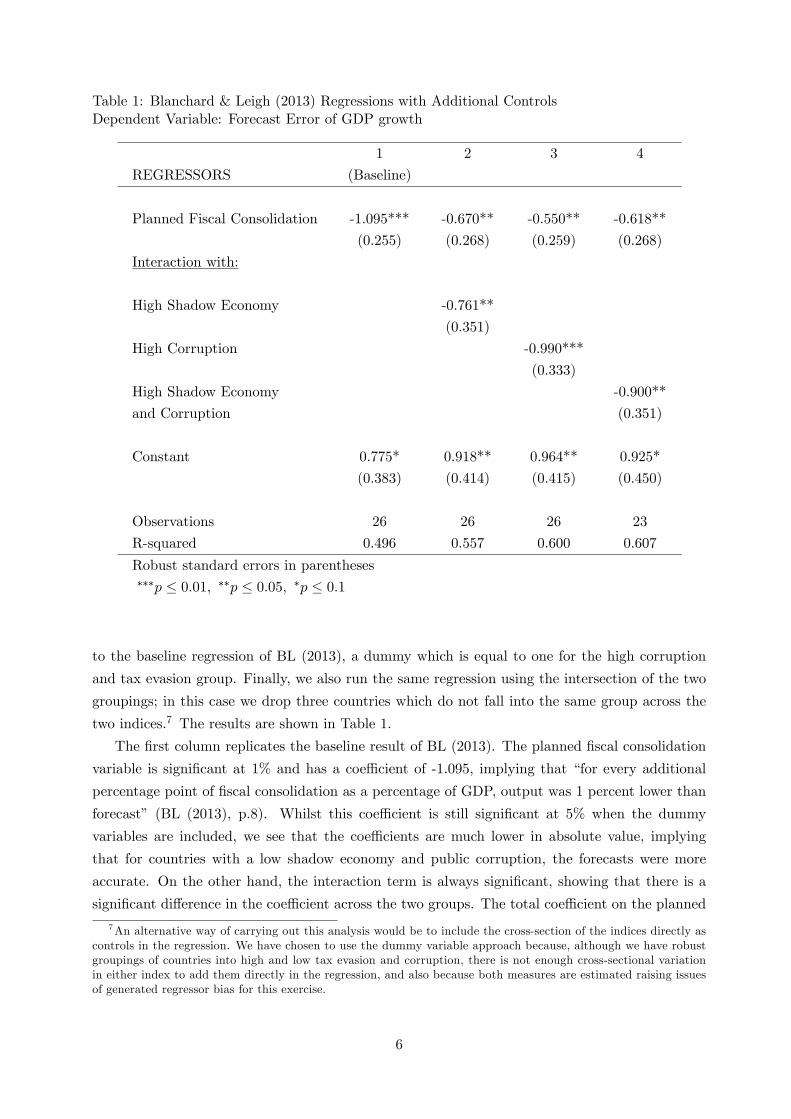
Table 1: Blanchard & Leigh (2013) Regressions with Additional ControlsDependent Variable: Forecast Error of GDP growth

1 2 3 4

REGRESSORS (Baseline)

Planned Fiscal Consolidation -1.095*** -0.670** -0.550** -0.618**

(0.255) (0.268) (0.259) (0.268)

Interaction with:

High Shadow Economy -0.761**

(0.351)

High Corruption -0.990***

(0.333)

High Shadow Economy -0.900**

and Corruption (0.351)

Constant 0.775* 0.918** 0.964** 0.925*

(0.383) (0.414) (0.415) (0.450)

Observations 26 26 26 23

R-squared 0.496 0.557 0.600 0.607

Robust standard errors in parentheses∗∗∗p ≤ 0.01, ∗∗p ≤ 0.05, ∗p ≤ 0.1

to the baseline regression of BL (2013), a dummy which is equal to one for the high corruption

and tax evasion group. Finally, we also run the same regression using the intersection of the two

groupings; in this case we drop three countries which do not fall into the same group across the

two indices.7 The results are shown in Table 1.

The first column replicates the baseline result of BL (2013). The planned fiscal consolidation

variable is significant at 1% and has a coeffi cient of -1.095, implying that “for every additional

percentage point of fiscal consolidation as a percentage of GDP, output was 1 percent lower than

forecast” (BL (2013), p.8). Whilst this coeffi cient is still significant at 5% when the dummy

variables are included, we see that the coeffi cients are much lower in absolute value, implying

that for countries with a low shadow economy and public corruption, the forecasts were more

accurate. On the other hand, the interaction term is always significant, showing that there is a

significant difference in the coeffi cient across the two groups. The total coeffi cient on the planned

7An alternative way of carrying out this analysis would be to include the cross-section of the indices directly ascontrols in the regression. We have chosen to use the dummy variable approach because, although we have robustgroupings of countries into high and low tax evasion and corruption, there is not enough cross-sectional variationin either index to add them directly in the regression, and also because both measures are estimated raising issuesof generated regressor bias for this exercise.

6

fiscal consolidation is -1.431 for the High Shadow Economy group, -1.540 for the High Corruption

group, and -1.518 for the High Shadow Economy and Corruption group. In all cases, this is well

above the baseline BL (2013) coeffi cient in absolute value, suggesting that the forecast errors were

significantly and systematically larger in these countries. In other words, the implicit underesti-

mation of fiscal multipliers is more pronounced in countries with a higher shadow economy and/or

corruption, suggesting that these two features amplify the effects of fiscal consolidations.

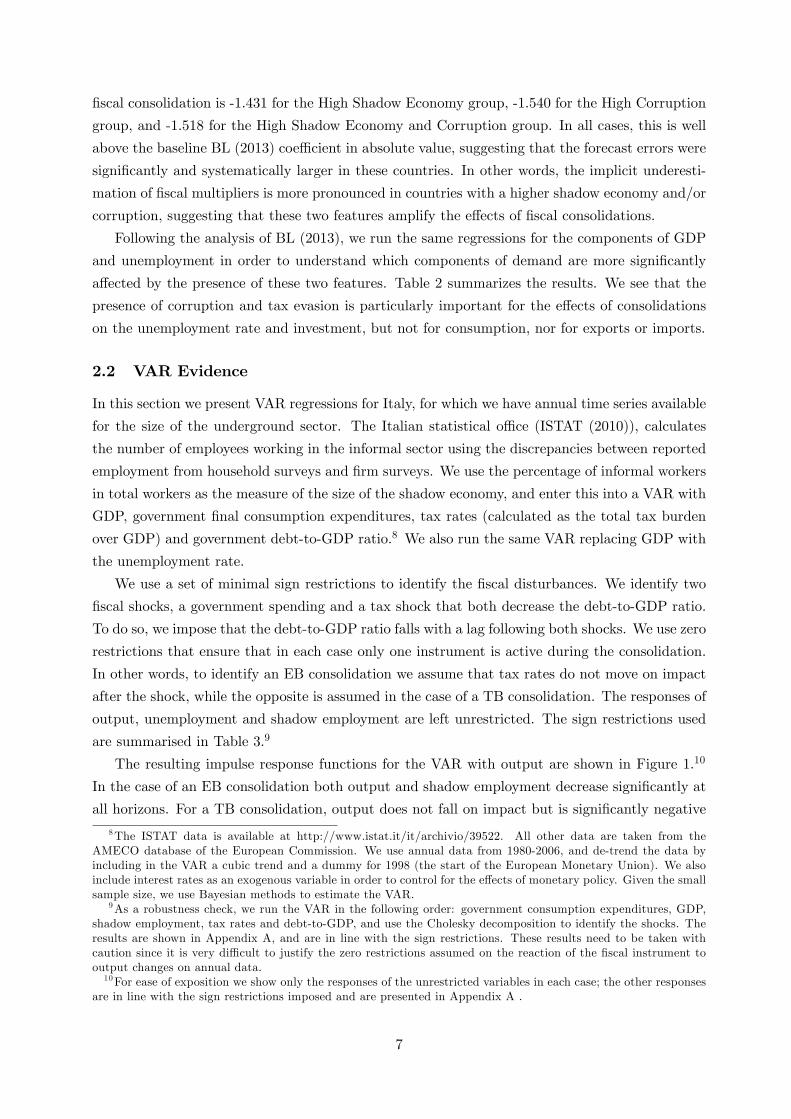
Following the analysis of BL (2013), we run the same regressions for the components of GDP

and unemployment in order to understand which components of demand are more significantly

affected by the presence of these two features. Table 2 summarizes the results. We see that the

presence of corruption and tax evasion is particularly important for the effects of consolidations

on the unemployment rate and investment, but not for consumption, nor for exports or imports.

2.2 VAR Evidence

In this section we present VAR regressions for Italy, for which we have annual time series available

for the size of the underground sector. The Italian statistical offi ce (ISTAT (2010)), calculates

the number of employees working in the informal sector using the discrepancies between reported

employment from household surveys and firm surveys. We use the percentage of informal workers

in total workers as the measure of the size of the shadow economy, and enter this into a VAR with

GDP, government final consumption expenditures, tax rates (calculated as the total tax burden

over GDP) and government debt-to-GDP ratio.8 We also run the same VAR replacing GDP with

the unemployment rate.

We use a set of minimal sign restrictions to identify the fiscal disturbances. We identify two

fiscal shocks, a government spending and a tax shock that both decrease the debt-to-GDP ratio.

To do so, we impose that the debt-to-GDP ratio falls with a lag following both shocks. We use zero

restrictions that ensure that in each case only one instrument is active during the consolidation.

In other words, to identify an EB consolidation we assume that tax rates do not move on impact

after the shock, while the opposite is assumed in the case of a TB consolidation. The responses of

output, unemployment and shadow employment are left unrestricted. The sign restrictions used

are summarised in Table 3.9

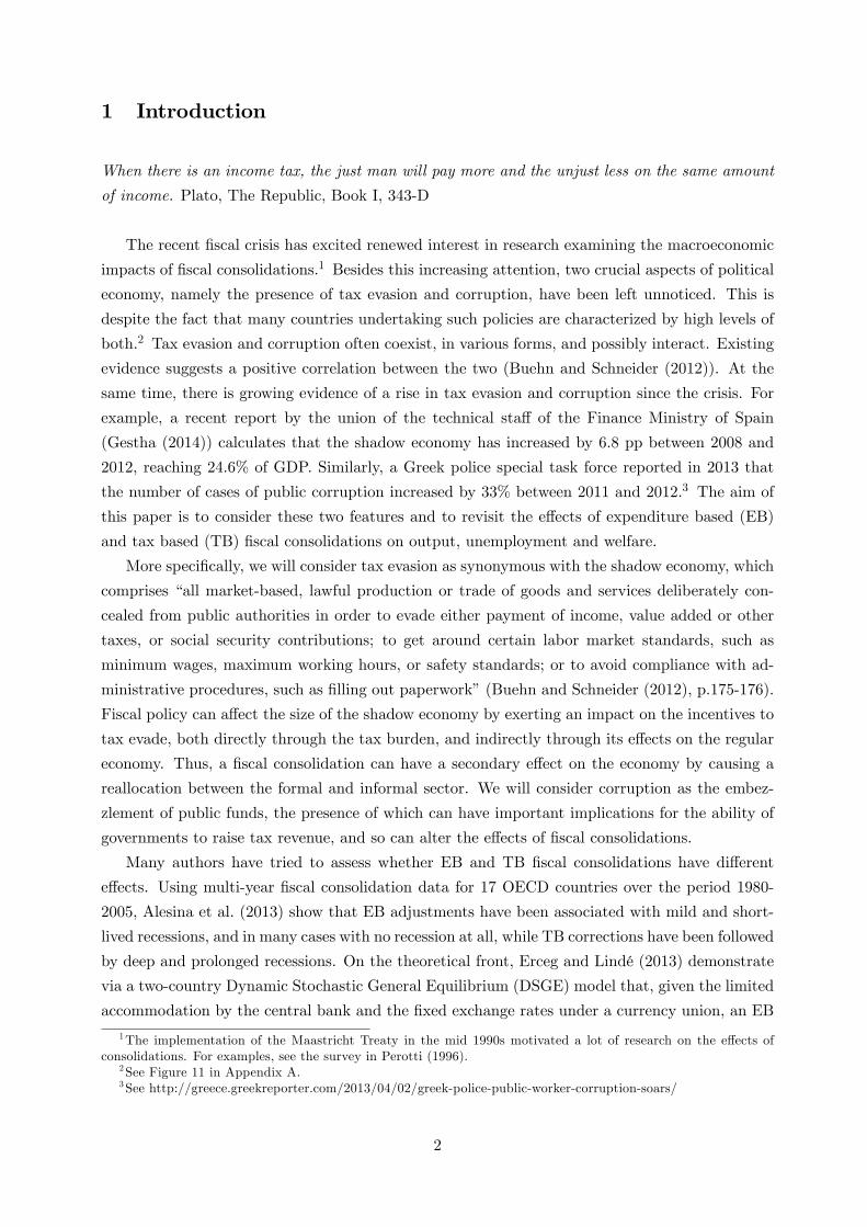
The resulting impulse response functions for the VAR with output are shown in Figure 1.10

In the case of an EB consolidation both output and shadow employment decrease significantly at

all horizons. For a TB consolidation, output does not fall on impact but is significantly negative

8The ISTAT data is available at http://www.istat.it/it/archivio/39522. All other data are taken from theAMECO database of the European Commission. We use annual data from 1980-2006, and de-trend the data byincluding in the VAR a cubic trend and a dummy for 1998 (the start of the European Monetary Union). We alsoinclude interest rates as an exogenous variable in order to control for the effects of monetary policy. Given the smallsample size, we use Bayesian methods to estimate the VAR.

9As a robustness check, we run the VAR in the following order: government consumption expenditures, GDP,shadow employment, tax rates and debt-to-GDP, and use the Cholesky decomposition to identify the shocks. Theresults are shown in Appendix A, and are in line with the sign restrictions. These results need to be taken withcaution since it is very diffi cult to justify the zero restrictions assumed on the reaction of the fiscal instrument tooutput changes on annual data.10For ease of exposition we show only the responses of the unrestricted variables in each case; the other responses

are in line with the sign restrictions imposed and are presented in Appendix A .

7

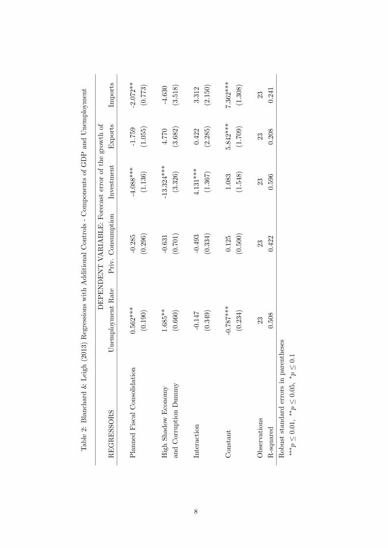
Table2:Blanchard&Leigh(2013)RegressionswithAdditionalControls-ComponentsofGDPandUnemployment

DEPENDENTVARIABLE:Forecasterrorofthegrowthof

REGRESSORS

UnemploymentRate

Priv.Consumption

Investment

Exports

Imports

PlannedFiscalConsolidation

0.562***

-0.285

-4.088***

-1.759

-2.072**

(0.190)

(0.296)

(1.136)

(1.055)

(0.773)

HighShadow

Economy

1.685**

-0.631

-13.324***

4.770

-4.630

andCorruptionDummy

(0.660)

(0.701)

(3.326)

(3.682)

(3.518)

Interaction

-0.147

-0.493

4.131***

0.422

3.312

(0.349)

(0.334)

(1.367)

(2.285)

(2.150)

Constant

-0.787***

0.125

1.083

5.842***

7.362***

(0.234)

(0.500)

(1.548)

(1.709)

(1.308)

Observations

2323

2323

23

R-squared

0.508

0.422

0.596

0.208

0.241

Robuststandarderrorsinparentheses

∗∗∗ p≤

0.0

1,∗∗p≤

0.05,∗ p≤

0.1

8

Table 3: Sign Restrictions

Variable: Govt Expenditure Tax Rate Debt-to-GDP

Shock: t = 0, 1 t = 0, 1 t = 2

Expenditure Cut — 0 —

Tax Hike 0 + —

in the long run, and there is a significant rise in shadow employment in the second period.

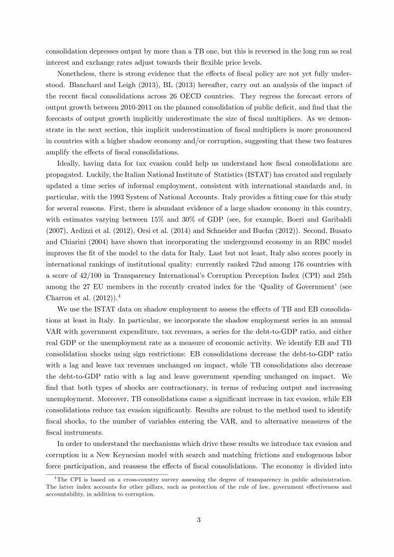
The results of the VAR with the unemployment rate are shown in Figure 2. We see that the

unemployment rate rises significantly after both types of consolidation, and, as before, shadow

employment falls in the case of an EB consolidation, and rises in the case of a TB consolidation.

We have also performed exercises, that we do not present here for economy of space, in which

we define the fiscal variables in the VAR as percentages of GDP, we replace GDP with a common

factor for economic activity and we include alternative series for the size of the shadow economy

provided by Elgin and Öztunah (2012). Results are robust to these changes.

Hence, the data robustly suggests that, for Italy, a consolidation through expenditure cuts

leads to a fall in shadow employment, whilst a consolidation through tax hikes increases shadow

employment. In the next section we construct a DSGE model with tax evasion and corruption and

try to replicate these empirical findings in order to understand the transmission of fiscal shocks

when the economy operates under such frictions.

3 The Model

We consider a DSGE model with search and matching frictions, endogenous labor decisions, and

sticky prices in the short run. Given that, in Section 2, we found no evidence that the presence

of corruption and tax evasion is important for understanding the effects of fiscal consolidation

on exports or imports, we consider a closed-economy model, thus, keeping the setup as simple

as possible. The economy is divided into the formal and the informal sector, and none of the

transactions occurring in the latter are recorded by government authorities. Firms therefore use

factors from underground markets to hide part of their production for tax evasion purposes. There

are two types of firms in the economy: (i) competitive intermediate firms that use capital and labor

to produce intermediate goods with two different technologies: one associated with the regular

sector and the other with the underground sector, and (ii) monopolistic competitive retailers that

use all intermediate varieties to produce differentiated retail goods, which are then aggregated

into a final consumption good. Price rigidities arise at the retail level, while search frictions

occur in the production of intermediate goods. In each period of time, intermediate firms face

a probability of being inspected by the fiscal authorities and convicted of tax evasion, in which

case they pay a penalty, and the employment match is terminated. There is a representative

household consisting of formal and informal employees, unemployed jobseekers and labor force

non-participants. Formal employment is subject to an income tax, whilst this tax is evaded by

9

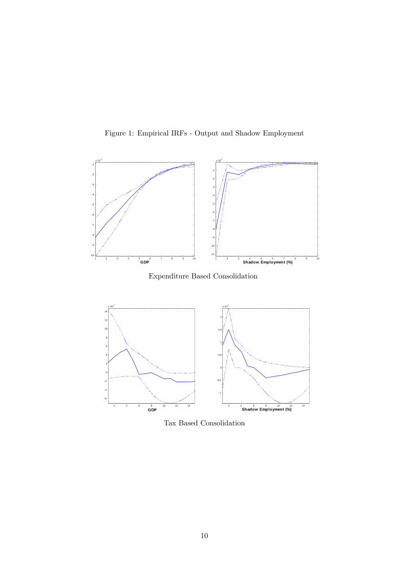
Figure 1: Empirical IRFs - Output and Shadow Employment

1 2 3 4 5 6 7 8 9 10­10

­9

­8

­7

­6

­5

­4

­3

­2

­1x 10­3

GDP1 2 3 4 5 6 7 8 9 10

­11

­10

­9

­8

­7

­6

­5

­4

­3

­2

­1

x 10­4

Shadow Employment (%)

Expenditure Based Consolidation

2 4 6 8 10 12 14

­6

­4

­2

0

2

4

6

8

10

12

14

x 10­3

GDP2 4 6 8 10 12 14

­1

­0.5

0

0.5

1

1.5

2

x 10­3

Shadow Employment (%)

Tax Based Consolidation

10

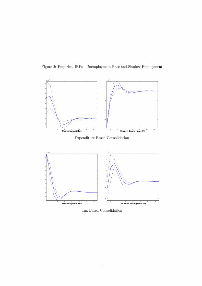
Figure 2: Empirical IRFs - Unemployment Rate and Shadow Employment

2 4 6 8 10 12 14

­2

0

2

4

6

8

10

12

14

x 10­4

Unemployment Rate2 4 6 8 10 12 14

­15

­10

­5

0

5x 10­4

Shadow Employment (%)

Expenditure Based Consolidation

2 4 6 8 10 12 14

­2

0

2

4

6

8

10

12

14

16

x 10­4

Unemployment Rate2 4 6 8 10 12 14

­6

­4

­2

0

2

4

6

8

x 10­4

Shadow Employment (%)

Tax Based Consolidation

11

the employees of the shadow economy. As well as their labor income, the household rents out

its private capital to the intermediate firms, and purchases the final consumption good. The

government collects taxes from the regular sector, embezzles a fraction of the revenues, and uses

the remainder to finance public expenditures and the provision of unemployment benefits.

3.1 Labor market

Following the literature on labor market frictions, we account for the imperfections and transaction

costs in the labor market by assuming that jobs are created through a matching function. For

j = F, I denoting the formal and informal sectors, we let υjt be the number of vacancies and ujt

the number of jobseekers in each sector. We assume matching functions of the form:

mjt = µj1(υjt )

µ2(ujt )1−µ2 (1)

where we allow for differences in the effi ciency of the matching process, µj1, in the two sectors. In

each sector we can define the probability of a jobseeker being hired, ψhjt , and of a vacancy being

filled, ψfjt , as well as the market tightness, θjt , as follows:

ψhjt ≡mjt

ujt, ψfjt ≡

mjt

υjt, θjt ≡

υjt

ujt

In each period, jobs in the formal sector are destroyed at a constant fraction, σF , and mFt new

matches are formed. The law of motion f formal employment, nFt , is thus given by:

nFt+1 = (1− σF )nFt +mFt (2)

In the informal sector there is an exogenous fraction of jobs destroyed in each period, σI , as well

as a probability that an informal employee might lose their job due to an audit, which we denote

by ρ. Therefore the law of motion of informal employment, nIt , is given by:

nIt+1 = (1− ρ− σI)nIt +mIt (3)

3.2 Households

The representative household is made up of a continuum of infinitely lived agents. The members

of the household derive utility from leisure, which corresponds to the fraction of members that

are out of the labour force, lt, and a consumption bundle, cct, defined as:

cct = [α1(ct)α2 + (1− α1)(gt)

α2 ]1α2 (4)

where gt denotes public consumption, which is taken as exogenous by the household, and

ct =[γ1(cFt )γ2 + (1− γ1)(cIt )

γ2] 1γ2 (5)

12

is the private consumption bundle, made up of the consumption goods produced in the formal

and informal sector. The elasticity of substitution between the private and public goods is given

by 11−α2

.11 Similarly, the elasticity of substitution between the formal and informal consumption

goods is given by 11−γ2

. The instantaneous utility function is given by:

U(cct, lt) =cc1−ηt

1− η + Φl1−ϕt

1− ϕ (6)

where η is the inverse of the intertemporal elasticity of substitution, Φ > 0 is the relative preference

for leisure, and ϕ is the inverse of the Frisch elasticity of labor supply.

At any point in time a fraction nFt (nIt ) of the representative household’s members are formal

(informal) employees. Campolmi and Gnocchi (2014), Brückner and Pappa (2012) and Bermper-

oglou et al. (2014) have added a labor force participation choice in New Keynesian models of

equilibrium unemployment. Following Ravn (2008), the participation choice is modelled as a

trade-off between the cost of giving up leisure and the prospect of finding a job. In particular, the

household chooses the fraction of the unemployed actively searching for a job, ut, and the fraction

which are out of the labor force and enjoying leisure, lt, so that:

nFt + nIt + ut + lt = 1 (7)

The household chooses the fraction of jobseekers searching in each sector: a share st of unemployed

looks for a job in the underground sector, while the remainder, (1− st), seek employment in theformal sector. That is, uIt ≡ stut and uFt ≡ (1− st)ut.

The household owns the capital stock, which evolves over time according to:

kt+1 = it + (1− δ)kt −ω

2

(kt+1

kt− 1

)2

kt (8)

where δ is a constant depreciation rate and ω2

(kt+1

kt− 1)2kt are adjustment costs.

The intertemporal budget constraint is given by:

(1 + τ ct)ct + it +Bt+1πt+1

Rt≤ rtkt + (1− τnt )wFt n

Ft + wIt n

It +$uFt +Bt + Πp

t − Tt (9)

where πt ≡ pt/pt−1 is the gross inflation rate, wjt , j = F, I , are the real wages in the two sectors, rt

is the real return to capital, $ denotes unemployment benefits, available only in the formal sector

(see Boeri and Garibaldi (2007)), Bt is the real government bond holdings, Rt is the gross nominal

interest rate, Πpt are the profits of the monopolistically competitive firms, discussed below, and τ

ct ,

τnt and Tt represent taxes on private consumption, labor income and lump-sum taxes respectively.

The household maximises expected lifetime utility subject to (1) for each j, (2), (3), (7), (8),

and (9). Taking as given njt , they choose ut, st (which together determine lt) and njt+1, as well as

ct, kt+1 and Bt+1.

11Recall the following limiting cases: when α2 approaches one, ct and gt are perfect substitutes. They are insteadperfect complements if α2 tends to minus infinity. α2 = 0 nests the Cobb-Douglas specification.

13

It is convenient to define the marginal value to the household of having an additional member

employed in the two sectors, as follows:

V hnF t = λctw

Ft (1− τnt )− Φl−ϕt + (1− σF )λnF t (10)

V hnI t = λctw

It − Φl−ϕt + (1− ρ− σI)λnI t (11)

where λnF t, λnI t and λct are the multipliers in front of (2), (3) and (9) respectively.12

3.3 Production

3.3.1 Intermediate goods firms

Intermediate goods are produced with two different technologies:

xFt = (AFt nFt )1−αF (kt)

αF (12)

xIt = (AItnIt )

1−αI (13)

where AFt > AIt denote total factor productivities. That is, we assume that the informal produc-

tion technology is less effi cient and uses labor inputs only (see e.g. Busato and Chiarini (2004)).

More importantly, since households consume a final good, we are also implicitly assuming that

the formal and informal goods are perfect substitutes. There is no differentiation between goods.

Final goods are produced with some intermediates that are not declared by the firms.

Firms maximize the discounted value of future profits, subject to (2) and (3), taking the

number of workers currently employed in each sector, njt , as given and choosing the number of

vacancies posted in the current period in each sector, υjt , so as to employ the desired number

of workers next period, njt+1. Here, firms adjust employment by varying the number of workers

(extensive margin) rather than the number of hours per worker (intensive margin). According to

Hansen (1985), most of the employment fluctuations arise from movements in this margin. Firms

also decide the amount of the private capital, kt , needed for production. They face a probability,

ρ , of being inspected by the fiscal authorities, convicted of tax evasion and forced to pay a penalty,

which is a fraction, γ , of their total revenues. Hence the problem of an intermediate firm is:

Q(njt ) = maxkt,υ

jt

(1− ργ) pxt (xFt + xIt )− (1 + τ st )w

Ft n

Ft − wIt nIt − rtkt − κFυFt − κIυIt + Et

[Λt,t+1Q(njt+1)

](14)

where pxt is the relative price of intermediate goods, τst is a payroll tax, κ

j is a cost associated

with posting a new vacancy in each sector j, and Λt,t+1 ≡ β Ucct+1

Ucct= β

(cct+1

cct

)−ηis a discount

12The first order conditions of the household’s problem and the derivations of equations (10) and (11) are presentedin the Appendix.

14

factor. The first-order conditions are:

rt = (1− ργ) pxt

(αFxFtkt

)(15)

κF

ψfFt= EtΛt,t+1

[(1− ργ) pxt+1(1− αF )

xFt+1

nFt+1

− (1 + τ st+1)wFt+1 +(1− σF )κF

ψfFt+1

](16)

κI

ψfIt= EtΛt,t+1

[(1− ργ) pxt+1(1− αI)

xIt+1

nIt+1

− wIt+1 +(1− ρ− σI)κI

ψfIt+1

](17)

According to (15)-(17), the net value of the marginal product of private capital should equal the

real rental rate and the marginal cost of opening a vacancy in each sector j should equal the

expected marginal benefit. The latter includes the net value of the marginal product of labor

minus the wage, augmented by the payroll tax in the formal sector, plus the continuation value.

Again for convenience we present the expected values of the marginal formal and informal job

for the intermediate firm:

V fnF t≡ ∂Q

∂nFt= (1− ργ) pxt (1− αF )

xFtnFt− (1 + τ st )w

Ft +

(1− σF )κF

ψfFt(18)

V fnI t≡ ∂Q

∂nIt= (1− ργ) pxt (1− αI)x

It

nIt− wIt +

(1− ρ− σI)κI

ψfIt(19)

3.3.2 Retailers

There is a continuum of monopolistically competitive retailers indexed by i on the unit interval.

Retailers buy intermediate goods and differentiate them with a technology that transforms one

unit of intermediate goods into one unit of retail goods, and thus the relative price of intermediate

goods, pxt , coincides with the real marginal cost faced by the retailers. Let yit be the quantity of

output sold by retailer i. The final consumption good can be expressed as:

yt =

[∫ 1

0(yit)

ε−1ε di

] εε−1

(20)

where ε > 1 is the constant elasticity of demand for retail goods. The final good is sold at its

price, pt =[∫ 1

0 p1−εit di

] 11−ε. The demand for each intermediate good depends on its relative price

and aggregate demand:

yit =

(pitpt

)−εyt (21)

Following Calvo (1983), we assume that in any given period each retailer can reset her price with

a fixed probability (1− χ). Hence, the price index is:

pt =[(1− χ)(p∗t )

1−ε + χ(pt−1)1−ε] 11−ε (22)

15

The firms that are able to reset their price, p∗it, choose it so as to maximize expected profits given

by:

Et

∞∑s=0

χsΛt,t+s(p∗it − pxt+s)yit+s

The resulting expression for p∗it is:

p∗it =ε

ε− 1

Et∑∞

s=0 χsΛt,t+sp

xt+syit+s

Et∑∞

s=0 χsΛt,t+syit+s

(23)

3.4 Government

The government’s expenditures consist of consumption purchases and unemployment benefits,

whilst their revenue comes from the collected fines and the payroll, consumption, and labor income

taxes, as well as the lump-sum taxes. The government deficit is therefore defined by:

DFt = gt +$uFt − (1− ξTR)TRt − ργpxt (xFt + xIt ) (24)

where TRt ≡ (τnt + τ st )wFt n

Ft + τ ctct +Tt represents the tax revenues and 0 ≤ ξTR < 1 denotes the

embezzlement rate in the presence of corruption in the economy.

The government budget constraint is defined by:

bt +DFtyt

= R−1t bt+1πt+1g

yt+1 (25)

where bt = Btytis the debt-to-GDP ratio and gyt+1 is the growth rate of GDP.

We assume transfers, Tt, , τ st , and τ ct are fixed at their steady-state level. Therefore the

government potentially has the following fiscal instruments Ψ ∈ g, τn, in line with Erceg andLindé (2013). Although we have tried to incorporate various types of distortionary taxation in our

framework, we present results for the varying labor tax only, since fiscal consolidations through

payroll tax hikes have very similar effects in our model and since consumption tax hikes, though

they have different effects from the other two types of taxes, do not constitute the major source

of tax revenues in any of the economies we study.

We consider each instrument separately, assuming that if one is active, the others remain fixed

at their steady-state levels. Following Erceg and Lindé (2013), we assume fiscal rules of the form:

Ψt = Ψ(1−βΨ0) ΨβΨ0t−1 exp(1− βΨ0)[βΨ1(bt − b∗t ) + βΨ2(∆bt+1 −∆b∗t+1)] (26)

where b∗t is the target value for this ratio and follows an AR(2) process:

log b∗t+1 − log b∗t = µb + ρ1(log b∗t − log b∗t−1)− ρ2 log b∗t + εbt (27)

where εbt is a white noise process with variance σε.

16

3.5 Closing the model

Monetary Policy There is an independent monetary authority that sets the nominal interest

rate as a function of current inflation according to the rule:

Rt = R expζπ(πt − 1) (28)

where R is the steady-state value of the nominal interest rate.

Goods Markets Total output must equal private and public demand. The resource constraint

for output is thus given by:

yt = ct + it + gt + κFυFt + κIυIt + ξTRTRt (29)

where the last term represents the resource costs in the economy due to corruption.13

The aggregate price index, pt, is given by (22) and (23). The return on private capital, rt,

adjusts so that the capital demanded by the intermediate goods firm, given by (15), is equal to

the stock held by the household.

Bargaining over wages Wages in both sectors are determined by ex post (after matching)

Nash bargaining. Workers and firms split rents and the part of the surplus they receive depends

on their bargaining power. For j = F, I we denote by ϑj ∈ (0, 1) the firms’bargaining power in

sector j. The Nash bargaining problem is to maximize the weighted sum of log surpluses:

maxwjt

(1− ϑj) log V h

njt + ϑj log V fnjt

where V h

njtand V f

njtare defined in equations (10), (11), (18) and (19). As shown in Appendix B.3,

wages are given by:

wFt =(1− ϑF )

(1 + τ st )

((1− ργ) pxt (1− αF )

xFtnFt

+(1− σF )κF

ψfFt

)+

ϑF

λct(1− τnt )

(Φl−ϕt −(1−σF )λnF t

)(30)

wIt = (1−ϑI)(

(1− ργ) pxt (1− αI)xIt

nIt+

(1− ρ− σI)κI

ψfIt

)+ϑI

λct

(Φl−ϕt − (1−ρ−σI)λnI t

)(31)

3.6 Calibration

We calibrate the model using annual data on the Italian economy over the period 1982-2006.14

Table 4 displays the values used for the different parameters. We calibrate the labor force partici-

pation and unemployment rate in the formal sector to match the observed average values from the

data. Thus we set offi cial labor force participation, lf = nF + uF , equal to 60% and the offi cial

13See Appendix B.2 for full derivations.14Details of the calibration exercise are in Appendix C.

17

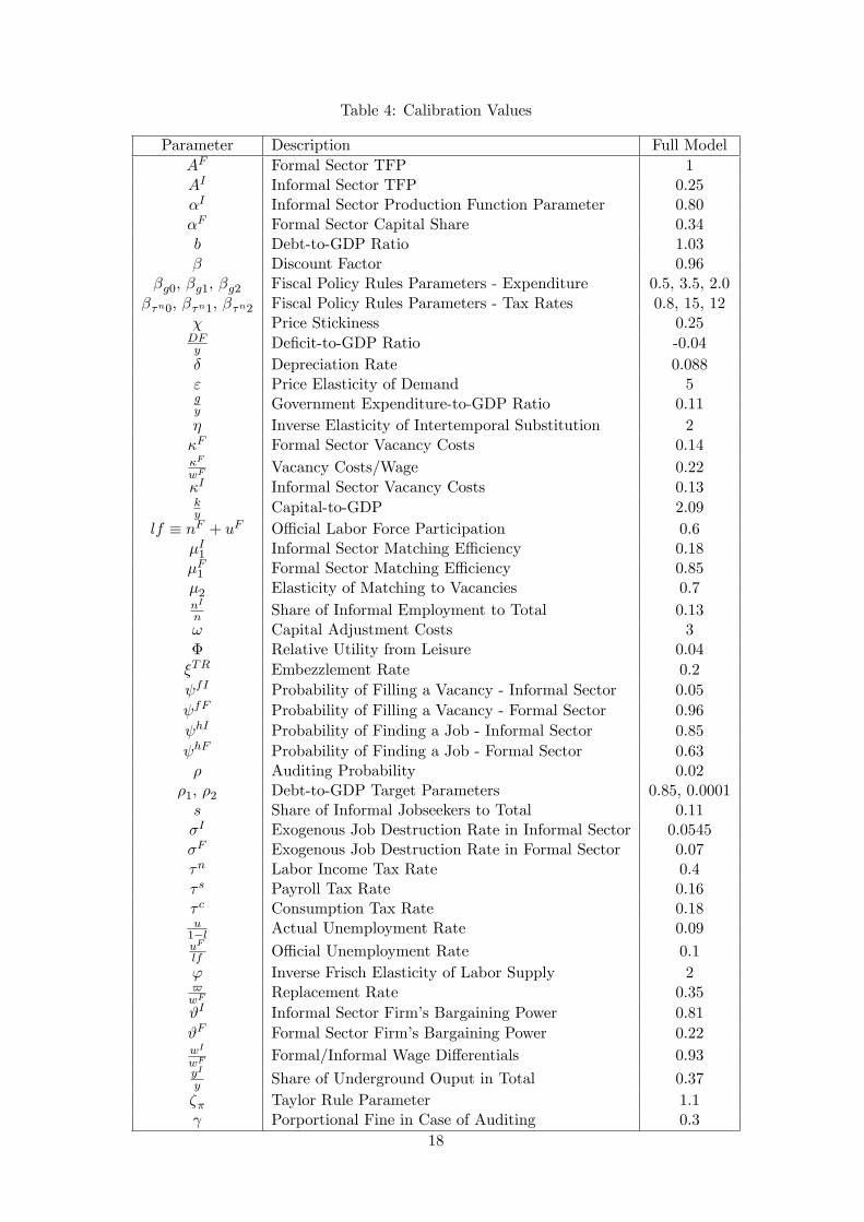
Table 4: Calibration Values

Parameter Description Full ModelAF Formal Sector TFP 1AI Informal Sector TFP 0.25αI Informal Sector Production Function Parameter 0.80αF Formal Sector Capital Share 0.34b Debt-to-GDP Ratio 1.03β Discount Factor 0.96

βg0, βg1, βg2 Fiscal Policy Rules Parameters - Expenditure 0.5, 3.5, 2.0βτn0, βτn1, βτn2 Fiscal Policy Rules Parameters - Tax Rates 0.8, 15, 12

χ Price Stickiness 0.25DFy Deficit-to-GDP Ratio -0.04δ Depreciation Rate 0.088ε Price Elasticity of Demand 5gy Government Expenditure-to-GDP Ratio 0.11η Inverse Elasticity of Intertemporal Substitution 2κF Formal Sector Vacancy Costs 0.14κF

wFVacancy Costs/Wage 0.22

κI Informal Sector Vacancy Costs 0.13ky Capital-to-GDP 2.09

lf ≡ nF + uF Offi cial Labor Force Participation 0.6µI1 Informal Sector Matching Effi ciency 0.18µF1 Formal Sector Matching Effi ciency 0.85µ2 Elasticity of Matching to Vacancies 0.7nI

n Share of Informal Employment to Total 0.13ω Capital Adjustment Costs 3Φ Relative Utility from Leisure 0.04ξTR Embezzlement Rate 0.2ψfI Probability of Filling a Vacancy - Informal Sector 0.05ψfF Probability of Filling a Vacancy - Formal Sector 0.96ψhI Probability of Finding a Job - Informal Sector 0.85ψhF Probability of Finding a Job - Formal Sector 0.63ρ Auditing Probability 0.02

ρ1, ρ2 Debt-to-GDP Target Parameters 0.85, 0.0001s Share of Informal Jobseekers to Total 0.11σI Exogenous Job Destruction Rate in Informal Sector 0.0545σF Exogenous Job Destruction Rate in Formal Sector 0.07τn Labor Income Tax Rate 0.4τ s Payroll Tax Rate 0.16τ c Consumption Tax Rate 0.18u

1−l Actual Unemployment Rate 0.09uF

lf Offi cial Unemployment Rate 0.1ϕ Inverse Frisch Elasticity of Labor Supply 2$wF

Replacement Rate 0.35ϑI Informal Sector Firm’s Bargaining Power 0.81ϑF Formal Sector Firm’s Bargaining Power 0.22wI

wFFormal/Informal Wage Differentials 0.93

yI

y Share of Underground Ouput in Total 0.37ζπ Taylor Rule Parameter 1.1γ Porportional Fine in Case of Auditing 0.3

18

unemployment rate to 10%. We fix the separation rate, σF , equal to 0.07. Since there is no exact

estimate for the value of the formal vacancy-filling probability, ψfF , in the literature, we use what

is considered as standard by setting it equal to 0.96. We set the matching elasticity with respect

to vacancies, µ2, equal to 0.7, close to the estimate for Italy in Peracchi and Viviano (2004).

The capital depreciation rate, δ, is set equal to 0.088. Following the literature, we set the

discount factor, β, equal to 0.96. The elasticity of demand for intermediate goods, ε, is set such

that the gross steady-state markup, εε−1 , is equal to 1.25, and the price of the final good is

normalized to one. The TFP parameter in the formal sector is normalized to one, AF = 1 and

the capital share αF = 0.34. The probability of audit and the fraction of total profits paid as a

fine in the event of an audit are set as follows: ρ = 0.02, which is close to the value used in Boeri

and Garibaldi (2007), and γ = 0.3. We set the vacancy costs in the formal sector κF = 0.14 and

the payroll tax rate τ s = 0.16, close to the value in Orsi et al. (2014).

In the informal sector, we assume that TFP is lower relative to the informal sector and set AI =

0.25. Using the ISTAT data, we set the share of underground employment to total employment

equal to 0.13. We set the value of αI equal to 0.8. We set the exogenous job destruction rate in

the informal sector σI = 0.0545 and set the probability of filling a vacancy in the informal sector

ψfI = 0.05 and the vacancy cost in the informal sector κI = 0.13.

Next, we set the replacement rate, $wF, equal to 0.35 close to the estimates in Martin (1996),

also used by Fugazza and Jacques (2004). Government spending as a share of GDP and the

tax rates are set as follows: gy = 11%, τn = 0.4, in line with Orsi et al. (2014), and τ c = 0.18.

The steady state debt-to-GDP ratio is taken from the data, b = 103%. We set the corruption

parameter ξTR = 0.2.

The intertemporal elasticity of substitution, 1η , is set equal to 0.5 and the inverse Frisch

elasticity, ϕ, equals 2. Finally, we set the inflation targeting parameter in the Taylor rule, ζπ = 1.1,

the capital adjustment costs ω = 3 and the price-stickiness parameter χ = 0.25. The fiscal policy

parameters are set so as to achieve a 5% drop in the debt-to-GDP target 10 periods after a debt

shock.

3.7 Results

We now present the impulse responses following a negative debt-target shock. We compare the

effects of a 5% reduction in the desired long-run debt target, which is achieved after 10 years,

either through a fall in consumption expenditure or a hike in the tax rates.

3.7.1 Benchmark Model

In order to understand how tax evasion and corruption affect the transmission of fiscal shocks,

we begin by analysing the response of the macroeconomy in a standard model where those two

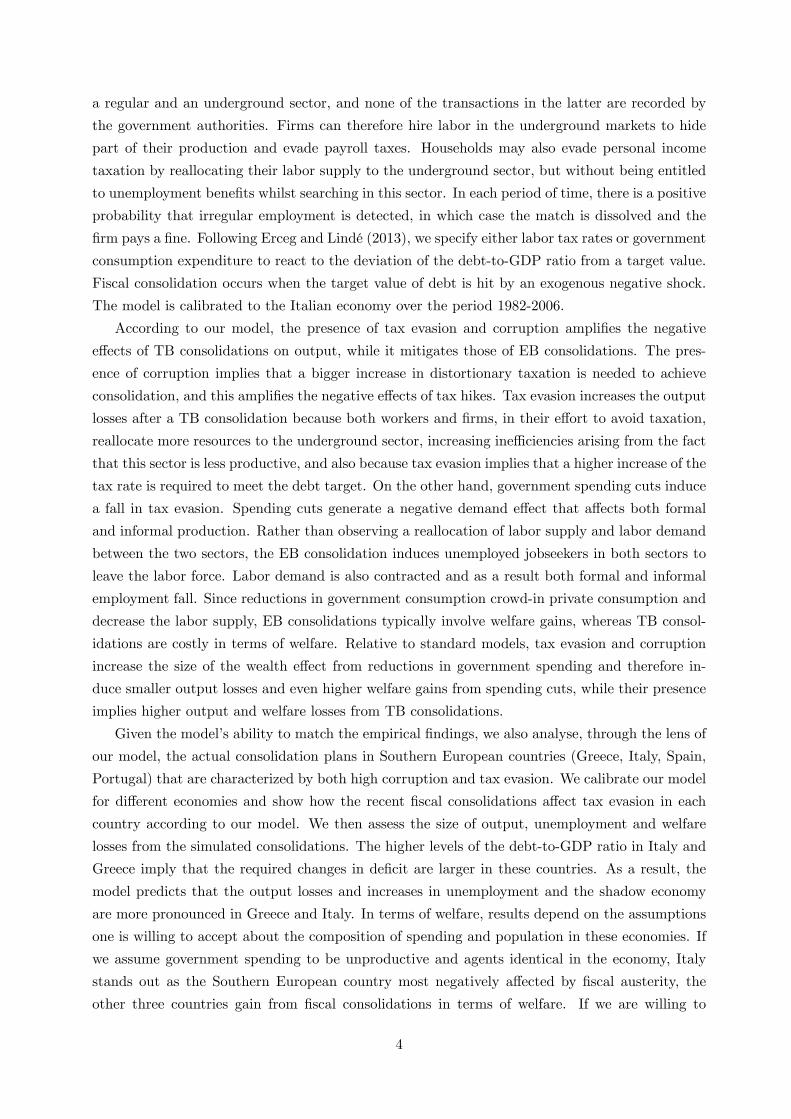
features are absent. The theoretical impulse responses are presented in Figure 3.

The consolidation carried out with a fall in government spending has two channels. First,

there is a negative demand effect, leading to a fall in labor demand, which is translated into

a fall in vacancies. Second, there is a positive wealth effect for the household, which increases

19

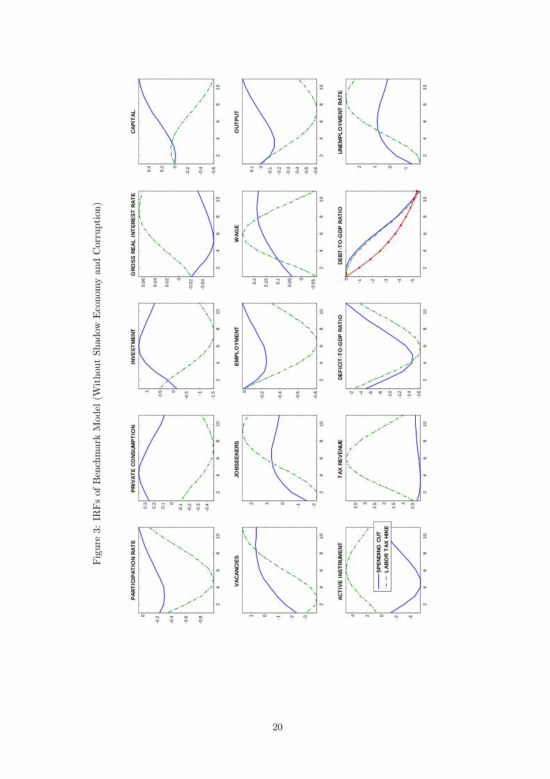
Figure3:IRFsofBenchmarkModel(WithoutShadow

EconomyandCorruption)

24

68

10

­0.8

­0.6

­0.4

­0.20

PART

ICIP

ATIO

N RA

TE

24

68

10

­0.4

­0.3

­0.2

­0.10

0.1

0.2

0.3

PRIV

ATE

CONS

UMPT

ION

24

68

10­1

.5­1

­0.50

0.51

INVE

STM

ENT

24

68

10

­0.0

4

­0.0

20

0.02

0.04

0.06

GRO

SS R

EAL

INTE

REST

RAT

E

24

68

10­0

.6

­0.4

­0.20

0.2

0.4

CAPI

TAL

24

68

10

­3­2­101

VACA

NCIE

S

24

68

10­2­1012

JOBS

EEKE

RS

24

68

10­0

.8

­0.6

­0.4

­0.20

EMPL

OYM

ENT

24

68

10

­0.0

50

0.050.

1

0.150.

2

WAG

E

24

68

10­0

.6

­0.5

­0.4

­0.3

­0.2

­0.10

0.1

OUT

PUT

24

68

10

­4­2024

ACTI

VE IN

STRU

MEN

T

24

68

10

0.51

1.52

2.53

3.5

TAX

REVE

NUE

24

68

10­1

6

­14

­12

­10­8­6­4­2

DEFI

CIT­

TO­G

DP R

ATIO

24

68

10

­5­4­3­2­10DE

BT­T

O­G

DP R

ATIO

24

68

10

­1012

UNEM

PLO

YMEN

T RA

TE

SPEN

DING

CUT

LABO

R TA

X HI

KE

20

consumption and investment and reduces labor force participation. Given the drop in both labor

demand and supply, employment falls and the wage increases. Output falls in the short run, but

increases in the medium and long run because of the increase in investment, which is translated

into an increase in the capital stock. The unemployment rate reflects the movement in the number

of jobseekers, which falls on impact, but then increases as employment adjusts.

When the fiscal consolidation is carried out through labor tax hikes, there is a negative wealth

effect for the household which reduces consumption. The fall in consumption induces a fall in

labor demand, expressed through a drop in vacancies. However, as the return from employment

falls, there is a substitution effect which outweighs the wealth effect, and there is again a decrease

in labor force participation. Employment and output fall, and the responses are significantly

larger and more persistent than in the case of spending cuts, given the delayed drop in investment

and, hence, capital.

Thus, the benchmark model confirms recent empirical evidence according to which EB con-

solidations are accompanied by mild and short-lived recessions, while TB consolidations lead to

more prolonged and deep recessions (see Alesina et al. (2013)).

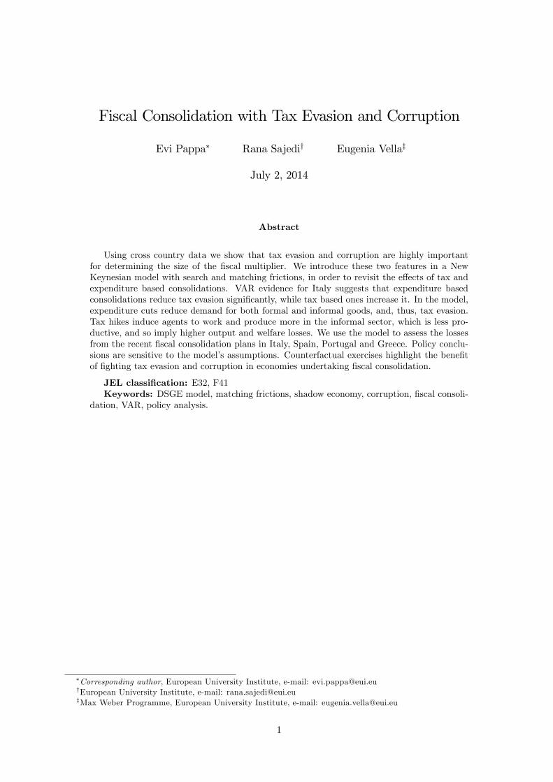
3.7.2 Model with Shadow Economy and Corruption

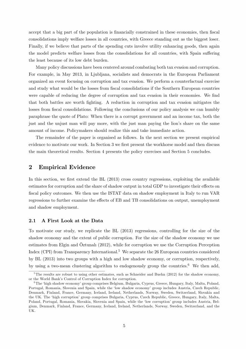
Next, we perform the same analysis for the economy with an underground sector and corruption.

Figure 4 depicts the formal sector and fiscal variables in this modified model, and Figure 5 shows

the underground sector.

First, we see from Figure 4 that the qualitative response of the formal sector is comparable

with that of the benchmark model. For the TB consolidation there is an additional channel

now at play as unemployed jobseekers reallocate their labor supply and the intermediate firms

reallocate their labor demand from the formal to the informal sector. Tax hikes provide direct

incentives for jobseekers to reallocate their search towards the underground sector because of the

higher tax rates associated with formal employment. At the same time, intermediate firms find it

profitable to reallocate the posted vacancies towards the underground sector because of the fall

in the informal wage, as shown in Figure 5. Consequently, employment and production in the

shadow economy increase.

The negative demand effect from spending cuts affects both formal and informal production.

Rather than observing a reallocation of labor supply and labor demand between the two sectors,

we see that unemployed jobseekers in both sectors decide to leave the labor force. Labor demand

is again contracted and as a result, formal and informal employment fall, replicating the responses

of the underground economy to a spending cut we observed for Italy in Subsection 2.2.

3.7.3 Comparisons and Sensitivity Analysis

Figure 6 shows the response of output, the unemployment rate and welfare for the benchmark

model and the model with tax evasion and corruption, for EB and TB consolidations separately, as

21

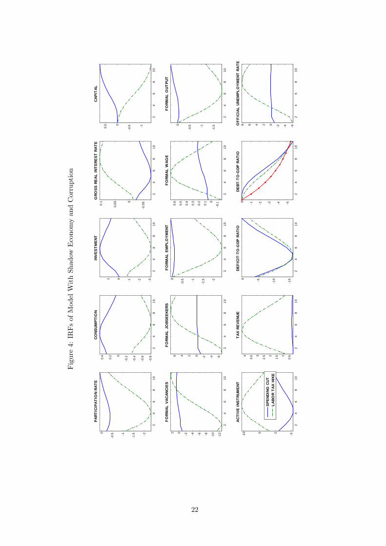
Figure4:IRFsofModelWithShadow

EconomyandCorruption

24

68

10

­2

­1.5­1

­0.50

PART

ICIP

ATIO

N RA

TE

24

68

10­0

.8

­0.6

­0.4

­0.20

0.2

0.4

CONS

UMPT

ION

24

68

10­3­2­101

INVE

STM

ENT

24

68

10

­0.0

50

0.050.

1G

ROSS

REA

L IN

TERE

ST R

ATE

24

68

10

­1

­0.50

0.5

CAPI

TAL

24

68

10

­12

­10­8­6­4­202

FORM

AL V

ACAN

CIES

24

68

10

­6­4­20246

FORM

AL J

OBS

EEKE

RS

24

68

10

­2

­1.5­1

­0.50

FORM

AL E

MPL

OYM

ENT

24

68

10

­0.10

0.1

0.2

0.3

0.4

0.5

0.6

FORM

AL W

AGE

24

68

10

­1.5­1

­0.50

FORM

AL O

UTPU

T

24

68

10­50510

ACTI

VE IN

STRU

MEN

T

24

68

10

0.51

1.52

2.53

3.54

TAX

REVE

NUE

24

68

10

­15

­10­50

DEFI

CIT­

TO­G

DP R

ATIO

24

68

10

­5­4­3­2­10DE

BT­T

O­G

DP R

ATIO

24

68

10­6­4­202468O

FFIC

IAL

UNEM

PLO

YM

ENT

RATE

SPEN

DING

CUT

LABO

R TA

X HI

KE

22

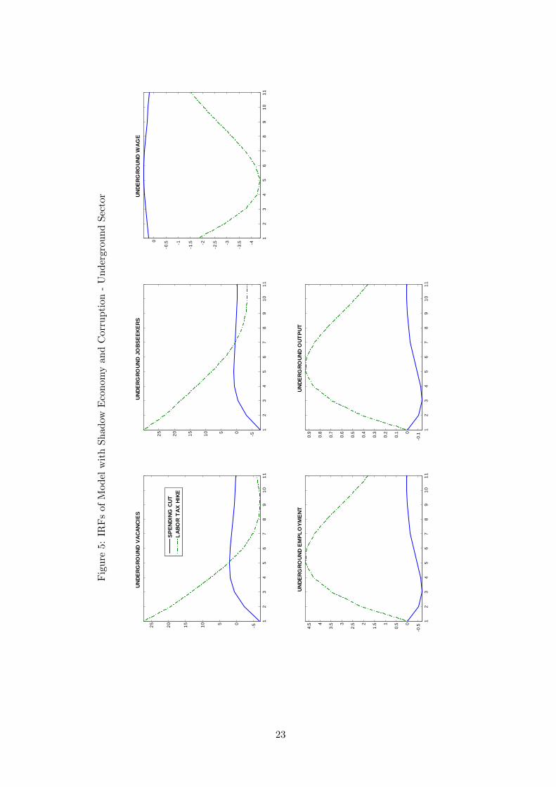
Figure5:IRFsofModelwithShadow

EconomyandCorruption-UndergroundSector

12

34

56

78

910

11

­50510152025

UNDE

RGRO

UND

VACA

NCIE

S

12

34

56

78

910

11

­50510152025

UNDE

RGRO

UND

JOBS

EEKE

RS

12

34

56

78

910

11

­4

­3.5­3

­2.5­2

­1.5­1

­0.50

UNDE

RGRO

UND

WAG

E

12

34

56

78

910

11

­0.50

0.51

1.52

2.53

3.54

4.5

UNDE

RGRO

UND

EMPL

OYM

ENT

12

34

56

78

910

11

­0.10

0.1

0.2

0.3

0.4

0.5

0.6

0.7

0.8

0.9

UNDE

RGRO

UND

OUT

PUT

SPEN

DING

CUT

LABO

R TA

X HI

KE

23

well as a mixed consolidation in which we allow both policy instruments to move simultaneously.15

We fix the relative contribution of expenditure cuts and revenue enhancements to the reduction

in deficit, based on the estimates of OECD (2012), which contains details of the recent fiscal

consolidation plans for many OECD countries. For Italy the reported share of expenditure cuts

in the consolidation plans is around 50%.

For spending cuts, shown in the top panel, we see that the presence of the shadow economy

yields smaller short run losses of output and decreases the unemployment rate at all horizons.

At the same time, consumption increases by more, and labor force participation falls by more,

relative to the benchmark case without tax evasion and corruption. This seems to suggest that

the presence of tax evasion and corruption amplifies the wealth effect. This is due to the fact

that, when tax evasion and corruption are present, the tax adjustments required to achieve a given

change in deficit are larger, and so, following a spending cut, taxes in the future are expected to

fall by more. The amplification of the wealth effect increases the crowding-in of the private sector

and reduces the negative demand effect of the fiscal contraction on output and unemployment.

We also see that in both models the EB consolidation implies welfare gains, and that allowing

for tax evasion and corruption increases welfare from EB consolidations. This is simply because

of the amplification of the wealth effect, which increases the crowding-in of private consumption

and the reduction of labor force participation.

For tax hikes, shown in the middle panel, we see that the presence of corruption and tax

evasion amplifies the output losses for many horizons, as the recession caused in the formal sector

is deeper. After the impact period, the rise in the offi cial unemployment rate is amplified. Finally,

we see that TB consolidation leads to welfare losses, because of the fall in consumption, which

are amplified by the presence of tax evasion and corruption.

For the mixed consolidation, depicted in the bottom panel, we see that, similarly to the case

of TB consolidation, the output losses and the increases in unemployment are amplified in the

presence of tax evasion and corruption. This is in line with the evidence from our extension of

the BL (2013) regressions in Section 2. Furthermore, the initial welfare gains are mitigated, but

this is reversed after 6 years.

Whilst the effects of TB consolidations are robust to a broad set of parameter values, the

effects of EB consolidations might depend crucially on some modelling assumptions. For instance,

spending cuts can result in welfare losses if government expenditures are assumed to be utility

enhancing. To investigate this, we conduct a sensitivity analysis by setting α1 = 0.85 and α2 =

−0.25, so that private and public spending are complements. Results from an EB consolidation

under this scenario are depicted in the top panel of Figure 7 in comparison to the case of wasteful

government spending.16 We see that output and unemployment effects are mitigated, while, as

expected, the response of welfare is reversed.

In addition, the presence of rule of thumb (ROT) consumers in the economy may imply smaller

15Welfare is computed as per-period steady state consumption equivalents. IRFs of all other variables are includedin Appendix A.16Note that, for comparison purposes, in all our exercises we adjust the parameters of the policy rules so that the

debt target is met after 10 years.

24

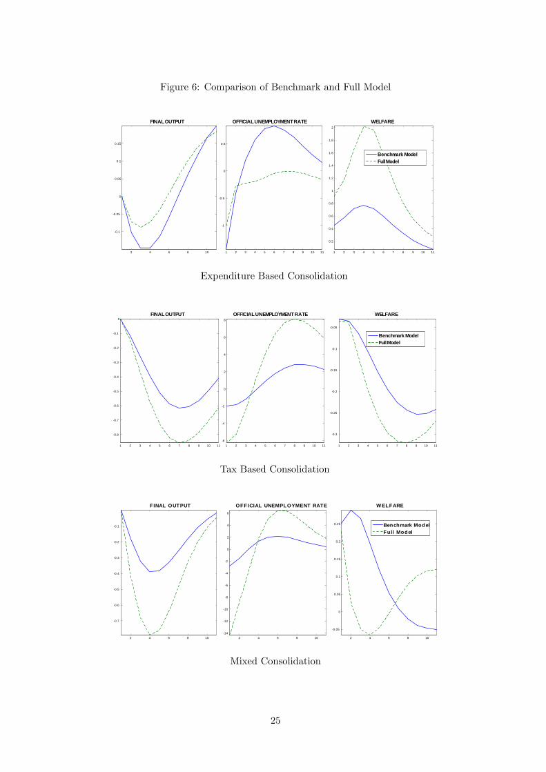
Figure 6: Comparison of Benchmark and Full Model

2 4 6 8 10

­0.1

­0.05

0

0.05

0.1

0.15

FINAL OUTPUT

1 2 3 4 5 6 7 8 9 10 11

­1

­0.5

0

0.5

OFFICIAL UNEMPLOYMENT RATE

1 2 3 4 5 6 7 8 9 10 11

0.2

0.4

0.6

0.8

1

1.2

1.4

1.6

1.8

2

WELFARE

Benchmark ModelFull Model

Expenditure Based Consolidation

1 2 3 4 5 6 7 8 9 10 11

­0.8

­0.7

­0.6

­0.5

­0.4

­0.3

­0.2

­0.1

0FINAL OUTPUT

1 2 3 4 5 6 7 8 9 10 11­6

­4

­2

0

2

4

6

8

OFFICIAL UNEMPLOYMENT RATE

1 2 3 4 5 6 7 8 9 10 11

­0.3

­0.25

­0.2

­0.15

­0.1

­0.05

WELFARE

Benchmark ModelFull Model

Tax Based Consolidation

2 4 6 8 10

­0.7

­0.6

­0.5

­0.4

­0.3

­0.2

­0.1

FINAL OUTPUT

2 4 6 8 10­14

­12

­10

­8

­6

­4

­2

0

2

4

6

OFFICIAL UNEMPLOYMENT RATE

2 4 6 8 10

­0.05

0

0.05

0.1

0.15

0.2

0.25

W ELFARE

Benchmark ModelFull Model

Mixed Consolidation

25

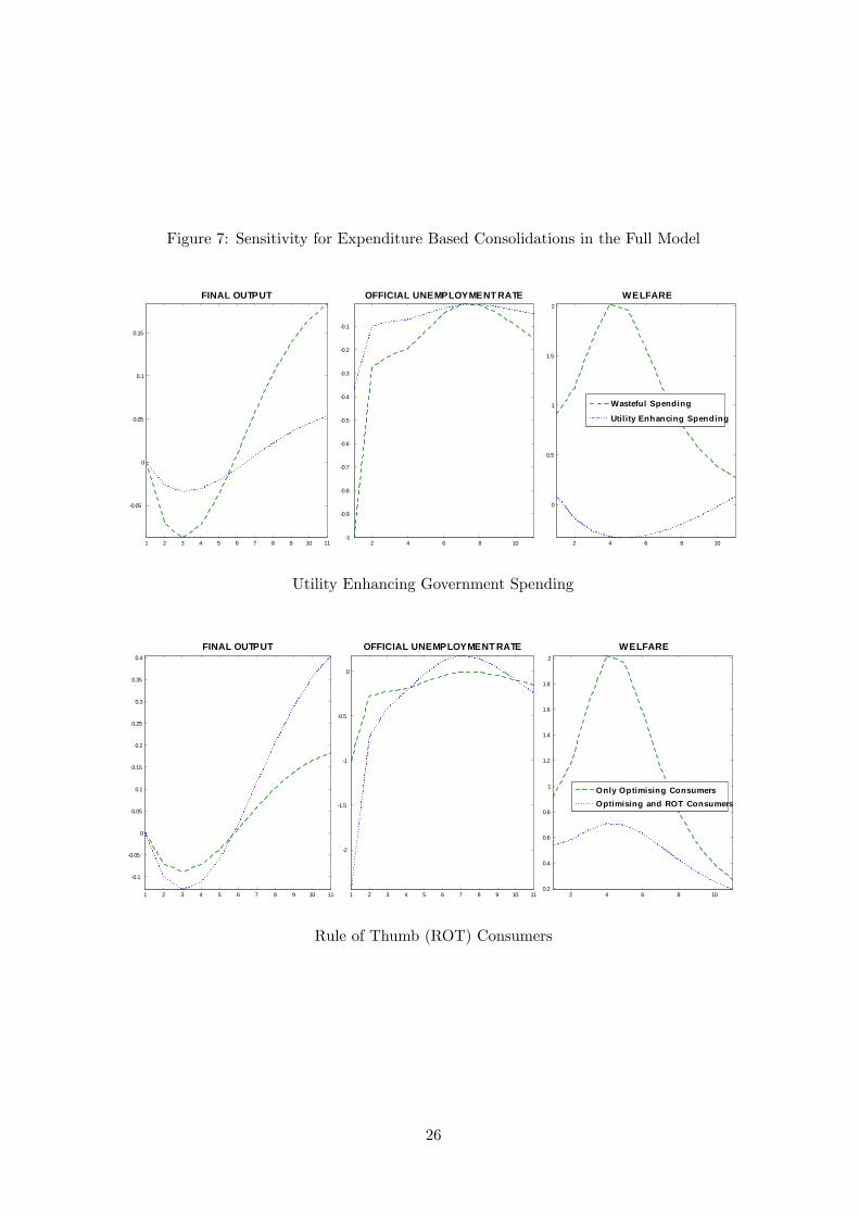
Figure 7: Sensitivity for Expenditure Based Consolidations in the Full Model

1 2 3 4 5 6 7 8 9 10 11

­0.05

0

0.05

0.1

0.15

FINAL OUTPUT

2 4 6 8 10­1

­0.9

­0.8

­0.7

­0.6

­0.5

­0.4

­0.3

­0.2

­0.1

OFFICIAL UNEMPLOYMENT RATE

2 4 6 8 10

0

0.5

1

1.5

2

WELFARE

Wasteful Spending

Utility Enhancing Spending

Utility Enhancing Government Spending

1 2 3 4 5 6 7 8 9 10 11

­0.1

­0.05

0

0.05

0.1

0.15

0.2

0.25

0.3

0.35

0.4

FINAL OUTPUT

1 2 3 4 5 6 7 8 9 10 11

­2

­1.5

­1

­0.5

0

OFFICIAL UNEMPLOYMENT RATE

2 4 6 8 100.2

0.4

0.6

0.8

1

1.2

1.4

1.6

1.8

2

WELFARE

Only Optimising ConsumersOptimising and ROT Consumers

Rule of Thumb (ROT) Consumers

26

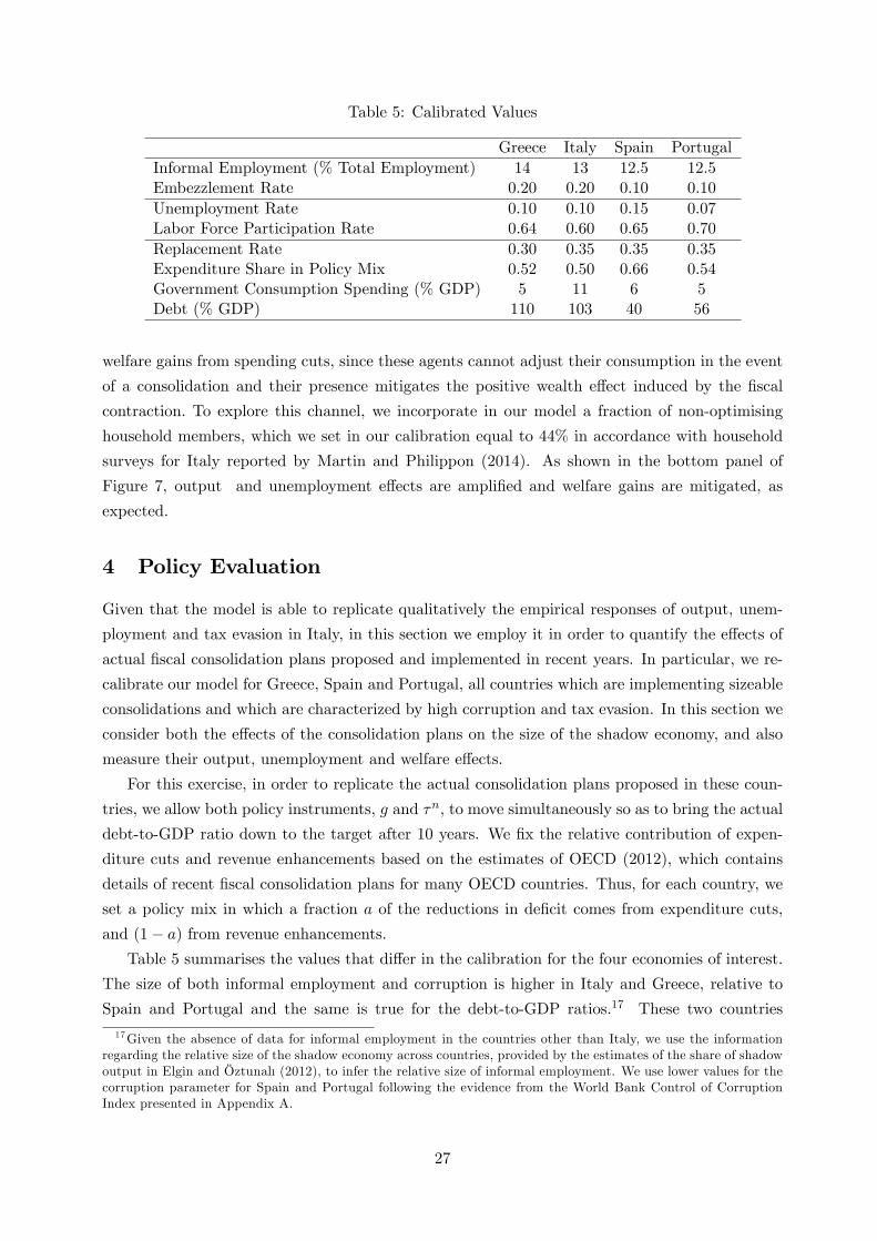
Table 5: Calibrated Values

Greece Italy Spain PortugalInformal Employment (% Total Employment) 14 13 12.5 12.5Embezzlement Rate 0.20 0.20 0.10 0.10Unemployment Rate 0.10 0.10 0.15 0.07Labor Force Participation Rate 0.64 0.60 0.65 0.70Replacement Rate 0.30 0.35 0.35 0.35Expenditure Share in Policy Mix 0.52 0.50 0.66 0.54Government Consumption Spending (% GDP) 5 11 6 5Debt (% GDP) 110 103 40 56

welfare gains from spending cuts, since these agents cannot adjust their consumption in the event

of a consolidation and their presence mitigates the positive wealth effect induced by the fiscal

contraction. To explore this channel, we incorporate in our model a fraction of non-optimising

household members, which we set in our calibration equal to 44% in accordance with household

surveys for Italy reported by Martin and Philippon (2014). As shown in the bottom panel of

Figure 7, output and unemployment effects are amplified and welfare gains are mitigated, as

expected.

4 Policy Evaluation

Given that the model is able to replicate qualitatively the empirical responses of output, unem-

ployment and tax evasion in Italy, in this section we employ it in order to quantify the effects of

actual fiscal consolidation plans proposed and implemented in recent years. In particular, we re-

calibrate our model for Greece, Spain and Portugal, all countries which are implementing sizeable

consolidations and which are characterized by high corruption and tax evasion. In this section we

consider both the effects of the consolidation plans on the size of the shadow economy, and also

measure their output, unemployment and welfare effects.

For this exercise, in order to replicate the actual consolidation plans proposed in these coun-

tries, we allow both policy instruments, g and τn, to move simultaneously so as to bring the actual

debt-to-GDP ratio down to the target after 10 years. We fix the relative contribution of expen-

diture cuts and revenue enhancements based on the estimates of OECD (2012), which contains

details of recent fiscal consolidation plans for many OECD countries. Thus, for each country, we

set a policy mix in which a fraction a of the reductions in deficit comes from expenditure cuts,

and (1− a) from revenue enhancements.

Table 5 summarises the values that differ in the calibration for the four economies of interest.

The size of both informal employment and corruption is higher in Italy and Greece, relative to

Spain and Portugal and the same is true for the debt-to-GDP ratios.17 These two countries

17Given the absence of data for informal employment in the countries other than Italy, we use the informationregarding the relative size of the shadow economy across countries, provided by the estimates of the share of shadowoutput in Elgin and Öztunalı(2012), to infer the relative size of informal employment. We use lower values for thecorruption parameter for Spain and Portugal following the evidence from the World Bank Control of CorruptionIndex presented in Appendix A.

27

also have smaller labor force participation rates, while the size of the government consumption

expenditures as a percentage of GDP is higher in Italy but lower in the other countries. In terms

of the consolidation packages, the mix between expenditure cuts and tax revenue increases looks

similar across the four economies, except for Spain that was dominated by expenditure cuts.

The results are shown in Figure 8.18 The high level of the debt-to-GDP ratio in Italy and

Greece implies that the required changes in taxation and government consumption spending and,

thus, deficit, are larger in these countries. As a result, after the fiscal consolidation, output

drops and the shadow economy increases by more in Greece and Italy. The same is true for

unemployment. Although the output and unemployment responses in Italy and Greece are similar,

Italy is the only country that suffers welfare losses in the medium run, as we saw in Figure 6.

This is due to the lower share of expenditure cuts in the consolidation mix, a = 0.5, and therefore

the higher increase in the tax rate, seen in the bottom left graph. In the other countries, fiscal

consolidations induce welfare gains. These welfare gains are higher in Portugal and Spain, where

the lower debt-to-GDP ratio implies smaller fiscal consolidations. For that reason, the effects

on output, unemployment and the shadow economy are qualitatively similar but quantitatively

smaller than in Italy and Greece.

As we saw previously, the presence of ROT consumers or utility enhancing government expen-

ditures can modify the predictions of the model regarding the welfare effects of fiscal consolidations.

For this reason, we examine the sensitivity of our policy evaluation conclusions when we incorpo-

rate these two features in our analysis. We use estimates for the fraction of ROT consumers across

the four countries from Martin and Philippon (2014), setting this parameter to 65% for Greece,

44% for Italy, 54% for Spain and 50% for Portugal. For the case of utility enhancing spending,

we again set α1 = 0.85 and α2 = −0.25 for all countries. The responses of welfare in each case

are shown in Figure 9.

The introduction of rule-of-thumb consumers overturns our previous policy evaluation conclu-

sions. First, the consolidation plans are associated with welfare losses for all countries, although

it is again true that Spain and Portugal are less affected relative to Italy and Greece. If we take

into account the presence of financially constrained individuals in the economy, Greece is the big

loser from fiscal consolidation among these countries since its share of rule of thumb consumers

is substantially higher relative to the other countries.

As expected, if government spending is assumed to complement private consumption, the

welfare losses from fiscal consolidations are large for all the countries we consider since in this

case both spending cuts and tax hikes negatively affect welfare. Under this scenario, the welfare

losses from fiscal consolidations are comparable in Greece, Italy and Portugal and are somewhat

smaller in the case of Spain, since the debt-to-GDP ratio is smaller in this country and smaller

sacrifices are needed to meet the debt target.

Given the emphasis in recent years on deterring tax evasion and corruption hand-in-hand with

carrying out fiscal consolidation, it is interesting to ask whether such reforms can change the

18Note that here we plot the deviation from steady state in levels, meaning, for example, that a value equal to1 on the vertical axis does not signify 101% of steady state, but rather 1 unit above steady state. In this way, wecontrol for the different steady states across countries, and responses are comparable.

28

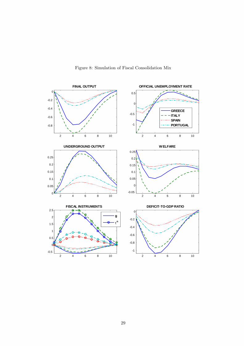
Figure 8: Simulation of Fiscal Consolidation Mix

2 4 6 8 10

­0.8

­0.6

­0.4

­0.2

0

FINAL OUTPUT

2 4 6 8 10

­1

­0.5

0

0.5

OFFICIAL UNEMPLOYMENT RATE

2 4 6 8 100

0.05

0.1

0.15

0.2

0.25

UNDERGROUND OUTPUT

2 4 6 8 10­0.05

0

0.05

0.1

0.15

0.2

0.25

W ELFARE

2 4 6 8 10­0.5

0

0.5

1

1.5

2

2.5FISCAL INSTRUMENTS

2 4 6 8 10

­1

­0.8

­0.6

­0.4

­0.2

0

DEFICIT­TO­GDP RATIO

g

τn

GREECEITALYSPAINPORTUGAL

29

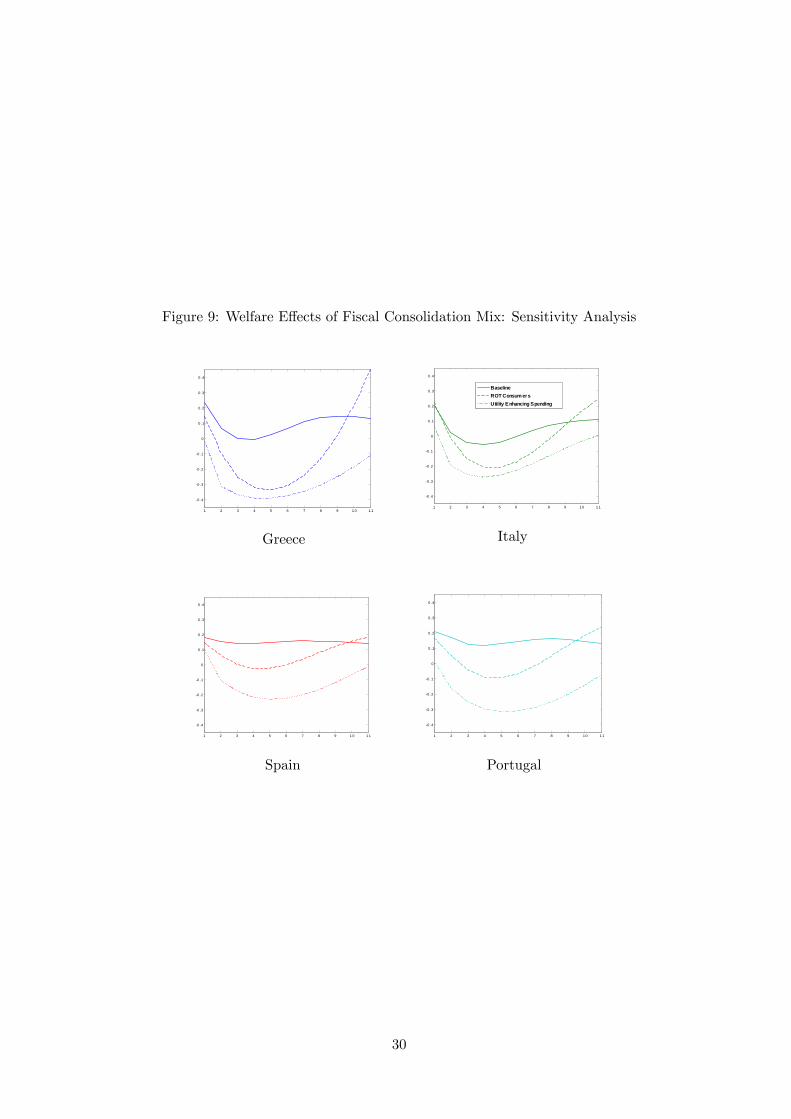
Figure 9: Welfare Effects of Fiscal Consolidation Mix: Sensitivity Analysis

1 2 3 4 5 6 7 8 9 1 0 1 1

­0 .4

­0 .3

­0 .2

­0 .1

0

0 .1

0 .2

0 .3

0 .4

Greece

1 2 3 4 5 6 7 8 9 1 0 1 1

­0 .4

­0 .3

­0 .2

­0 .1

0

0 .1

0 .2

0 .3

0 .4

BaselineROT Consum ersUtility Enhancing Spending

Italy

1 2 3 4 5 6 7 8 9 1 0 1 1

­0 .4

­0 .3

­0 .2

­0 .1

0

0 .1

0 .2

0 .3

0 .4

Spain

1 2 3 4 5 6 7 8 9 1 0 1 1

­0 .4

­0 .3

­0 .2

­0 .1

0

0 .1

0 .2

0 .3

0 .4

Portugal

30

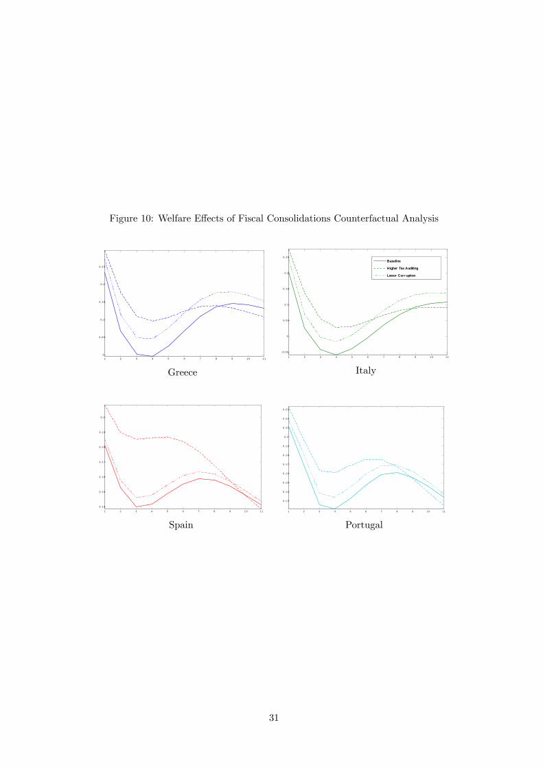
Figure 10: Welfare Effects of Fiscal Consolidations Counterfactual Analysis

1 2 3 4 5 6 7 8 9 1 0 1 10

0 .0 5

0 .1

0 .1 5

0 .2

0 .2 5

Greece

1 2 3 4 5 6 7 8 9 1 0 1 1

­0 .0 5

0

0 .0 5

0 .1

0 .1 5

0 .2

0 .2 5

Baseline

Higher Tax Auditing

Lower Cor ruption

Italy

1 2 3 4 5 6 7 8 9 1 0 1 1

0 .1 4

0 .1 5

0 .1 6

0 .1 7

0 .1 8

0 .1 9

0 .2

Spain

1 2 3 4 5 6 7 8 9 1 0 1 1

0 .1 3

0 .1 4

0 .1 5

0 .1 6

0 .1 7

0 .1 8

0 .1 9

0 .2

0 .2 1

0 .2 2

0 .2 3

Portugal

31

effects of the consolidation plans currently being implemented. In order to investigate this, we

use our model to carry out a counterfactual experiment. In particular, we again simulate the

fiscal consolidation plans for the four economies, this time assuming that the auditing probability

for tax evasion is double that of the previous calibration. Figure 10 depicts, for each country,

the welfare losses in the baseline calibration with solid lines and when the auditing probability is

higher with dashed lines. We see that since output losses are mitigated, for all of the countries,

welfare gains are amplified. Moreover, the medium-run welfare losses in Italy become welfare

gains, given that fighting tax evasion implies lower hikes in the tax rates needed to achieve the

targeted consolidation.

In a similar manner, we carry out a counterfactual experiment, this time reducing by 50%

the embezzlement rate, and so reducing the extent of corruption, in the underlying economies.

Welfare losses are depicted with dotted lines in Figure 10. Reducing corruption improves welfare

during the consolidations for all countries and most significantly so for Italy, where medium run

welfare losses become very small, and Greece, since these two countries are calibrated to have a

higher degree of public corruption. These results suggest that there should be an emphasis on

fighting public corruption, particularly in the time of a consolidation, since output losses can be

mitigated and welfare gains can be amplified significantly when healthier public institutions are

in place.

5 Concluding Remarks

Cross country regressions suggest clearly that accounting for both tax evasion and corruption

is key to understanding the effects of fiscal policy. Through a New Keynesian DSGE model

with involuntary unemployment, an underground sector and corruption, we have been able to

show that the presence of tax evasion and corruption amplifies the contractionary effects of tax

based consolidations, whilst it mitigates the effects of expenditure based ones. Moreover, the

type of fiscal consolidation affects the incentives of agents to produce in the shadow sector. In

particular, expenditure based consolidations reduce the size of the shadow economy, whilst tax

based consolidations increase it. These results match VAR evidence for Italy for which data on

informal employment exists.

Given the model’s ability to reproduce qualitatively the data patterns, we proceed to analyse

the output, unemployment and welfare effects of actual fiscal consolidation plans in Italy, Greece,

Spain and Portugal. Fiscal consolidations imply sizeable output and unemployment losses in

Greece and Italy, both because these countries are characterized by higher level of public cor-

ruption and tax evasion, and also because the debt burden in these countries is higher, requiring

higher sacrifices to achieve consolidation. Our policy conclusions depend on which assumptions

one is willing to take on board as more realistic for describing these four economies. If government

spending is assumed to be wasteful and we further assume that all agents are optimizers in the

economy, Italy stands as the only loser from the fiscal consolidations in the medium run, because

its consolidation mix relies more heavily on tax hikes. If we are willing to accept that some of the

government spending cuts involve goods that are complements to private consumption, then the

32

welfare losses from austerity are large for all countries and Spain is the country suffering the least

from these packages because its fiscal adjustment was limited. Finally, if we assume that agents

are financially constrained in these countries, as suggested by Martin and Philippon (2014), then

fiscal consolidations involve welfare costs for all countries and these are higher for Greece and

Italy.

Given the recent policy concerns about the reduction of both tax evasion and corruption in

Europe and the commitment of politicians to reduce both, we perform a counterfactual exercise

in order to evaluate the impact of such reforms on the output, unemployment and welfare losses.

The model predicts that fighting both public corruption and tax evasion should be at the top of

the list of reforms government should pursue in order to reduce the costs of fiscal consolidations.

We view our exercise as a first attempt in analysing the effects of corruption and tax evasion

on the size of the fiscal multiplier. Our model is stylistic and we have left out many important

aspects that could affect our conclusions. For example, in our economy we consider a representative

household and we cannot assess the effects of tax evasion and corruption on income inequality.

Also, we consider only cuts in government consumption expenditures and not in other items of

the government budget. Similarly, we consider only hikes in labor income taxes and not in other

sources of tax revenue. Furthermore, our framework does not allow for tax evasion on consumption

taxes, which is present in many economies. Finally, we do not endogenize the degree of public

corruption and we do not make it interact with aspects of the political economy, such as the

existence of two major predominant parties in the countries under consideration. We leave these

issues for future research.

33

References

[1] Alesina A., C. Favero. and F. Giavazzi, 2013, ‘The output effect of fiscal consolidations’,

Working Papers 478, IGIER, Bocconi University.

[2] Ardizzi G., C. Petraglia, M. Piacenza and G. Tutati, 2012, ‘Measuring the underground

economy with the currency demand approach: A reinterpretation of the methodology, with

an application to Italy’, Bank of Italy Working Paper Series, No. 864.

[3] Bermperoglou D., E. Pappa and E. Vella, 2013, ‘Spending cuts and their effects on output,

unemployment and the deficit’, manuscript.

[4] Blanchard, O. and D. Leigh, 2013, ‘Growth Forecast Errors and Fiscal Multipliers’, IMF

Working Papers 13/1.

[5] Boeri T. and P. Garibaldi, 2007, ‘Shadow sorting,’NBER International Seminar on Macro-

economics 2005, MIT Press, 125-163.

[6] Brückner, M. and E. Pappa, 2012, ‘Fiscal Expansions, Unemployment, and Labor Force

Participation: Theory and Evidence’, International Economic Review, 53(4), 1205-1228.

[7] Buehn A. and F. Schneider, 2012, ‘Corruption and the shadow economy: like oil and vinegar,

like water and fire?’, International Tax and Public Finance, 19(1), 172-194.

[8] Busato F. and B. Chiarini, 2004, ‘Market and underground activities in a two-sector dynamic

equilibrium model’, Economic Theory, 23(4), 831-861.

[9] Campolmi A. and S. Gnocchi, 2014, ‘Labor market participation, unemployment and mone-

tary policy’, Bank of Canada Working Paper No. 2014/9.

[10] Charron N., V. Lapuente and L. Dijkstra, 2012, ‘Regional governance matters: A study

on the regional variation in quality of government within the EU’, European Commission

Working Paper Series No. 01/2012.

[11] Elgin C. and O. Öztunah O., 2012, ‘Shadow economies around the world: Model based

estimates’, working paper.

[12] Erceg, C. and J. Lindé, 2013, ‘Fiscal consolidation in a currency union: Spending cuts vs.

tax hikes,’Journal of Economic Dynamics and Control, 37(2), 422-445.

[13] Fugazza M. and J.-F. Jacques, 2004, ‘Labor market institutions, taxation and the under-

ground economy,’Journal of Public Economics, 88, 395-418.

[14] Gestha, 2014, ‘La economía sumergida pasa factura. El avance del fraude en España durante

la crisis’, Madrid, enero de 2014.

34

[15] Hansen G., 1985, ‘Indivisible labor and the business cycle,’Journal of Monetary Economics,

16, 309-27.

[16] ISTAT, 2010, ‘La misura dell’economia sommersa secondo le statistiche uffi cialli. Anni 2000-

2008,’Conti-Nazionali-Statistiche in Breve, Istituto Nazionale di Statistica, Rome.

[17] Kolm A. and B. Larsen, 2003, ‘Social norm, the informal sector and unemployment,’Finan-

zArchiv, 59, 407-424.

[18] Martin J., 1996, ‘Measures of replacement rates for the purpose of international comparison:

A note’, OECD Economic Studies, 26(1), 98-118.

[19] Martin, P. and T. Philippon, 2014, ‘Inspecting the Mechanism: Leverage and the Great

Recession in the Eurozone,’Unpublished Manuscript.

[20] OECD, 2012, Restoring Public Finances, 2012 Update, OECD Publishing.

http://dx.doi.org/10.1787/9789264179455-en

[21] Orsi R., D. Raggi and F. Turino, 2014, ‘Size, trend, and policy implications of the under-

ground economy’, forthcoming in the Review of Economic Dynamics.

[22] Peracchi F. and E. Viviano, 2004, ‘An empirical micro matching model with an application

to Italy and Spain’, Temi di discussione No. 538, Banca d Italia.

[23] Perotti R., 1996, ‘Fiscal consolidation in the Europe: Composition matters’, American Eco-

nomic Review Papers and Proceedings, 86(2), 105-110.

[24] Ravn, M. O., 2008, ‘The Consumption-Tightness Puzzle’, NBER Chapters, NBER Interna-

tional Seminar on Macroeconomics 2006, 9-63.

[25] Schneider F. and A. Buehn, 2012, ‘Shadow economies in highly developed OECD countries:

What are the driving forces?’, IZA discussion paper No. 6891, Institute for the study of labor,

University of Bonn, Bonn, 2012.

35

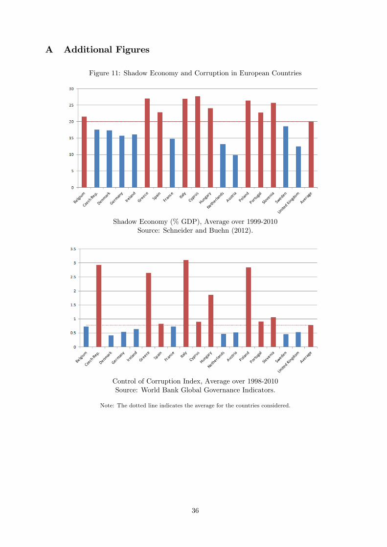
A Additional Figures

Figure 11: Shadow Economy and Corruption in European Countries

Shadow Economy (% GDP), Average over 1999-2010Source: Schneider and Buehn (2012).

Control of Corruption Index, Average over 1998-2010Source: World Bank Global Governance Indicators.

Note: The dotted line indicates the average for the countries considered.

36

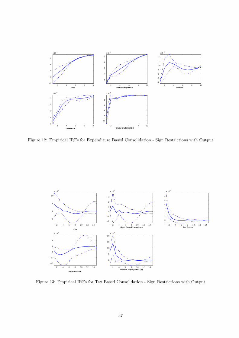
2 4 6 8 10­10

­8

­6

­4

­2

x 10 ­3

GDP2 4 6 8 10

­5

­4

­3

­2

­1

x 10 ­3

Govt Cons Expenditure2 4 6 8 10

­4

­3

­2

­1

0

1

2

x 10 ­4

Tax Rates

2 4 6 8 10­5

­4

­3

­2

­1

x 10 ­3

Debt­to­GDP2 4 6 8 10

­10

­8

­6

­4

­2

x 10 ­4

Shadow Employment (%)

Figure 12: Empirical IRFs for Expenditure Based Consolidation - Sign Restrictions with Output

2 4 6 8 10 12 14

­5

0

5

10

x 10­3

GDP

2 4 6 8 10 12 14

­2

­1

0

1

2

3

x 10­3

Govt C ons Expenditure2 4 6 8 10 12 14

0

1

2

3

4

5

6

x 10­3

Tax R ates

2 4 6 8 10 12 14

­15

­10

­5

0

5

x 10­3

D ebt­to­GD P

2 4 6 8 10 12 14

0

5

10

15

20x 10­4

Shadow Employment (%)

Figure 13: Empirical IRFs for Tax Based Consolidation - Sign Restrictions with Output

37

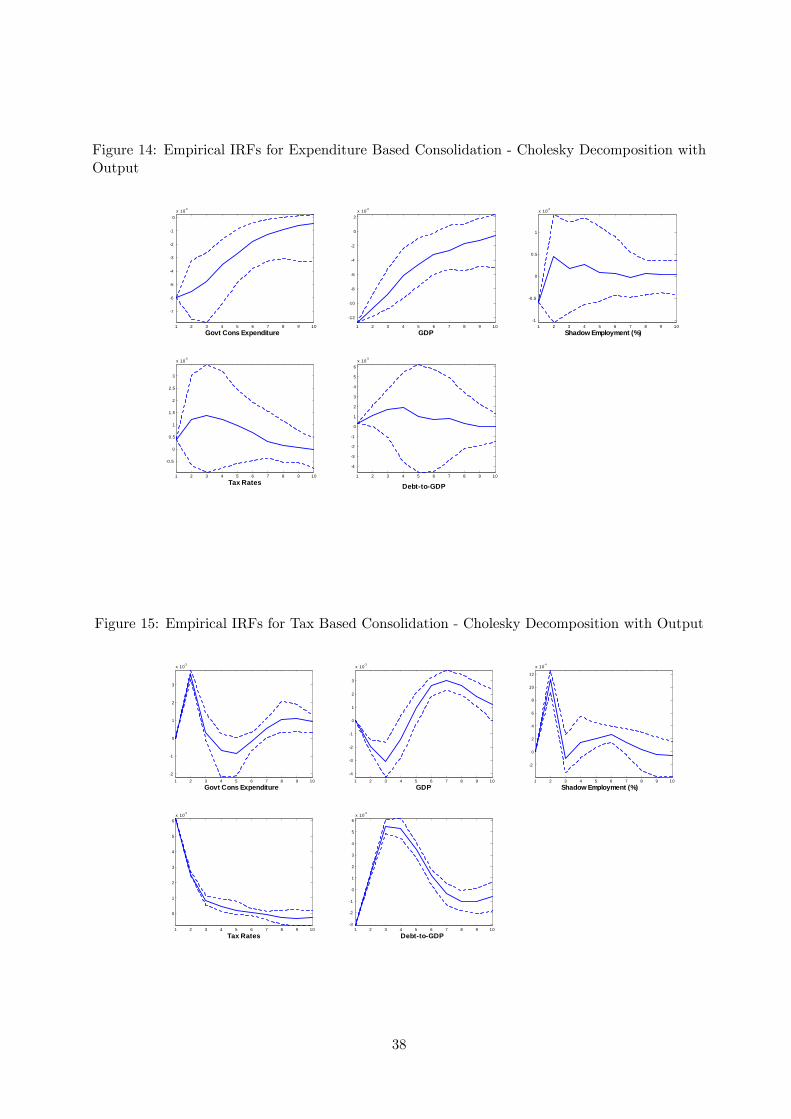
Figure 14: Empirical IRFs for Expenditure Based Consolidation - Cholesky Decomposition withOutput

1 2 3 4 5 6 7 8 9 10

­7

­6

­5

­4

­3

­2

­1

0x 10­3

Govt Cons Expenditure1 2 3 4 5 6 7 8 9 10

­12

­10

­8

­6

­4

­2

0

2x 10­3

GDP1 2 3 4 5 6 7 8 9 10

­1

­0.5

0

0.5

1

x 10­3

Shadow Employment (%)

1 2 3 4 5 6 7 8 9 10

­0.5

0

0.5

1

1.5

2

2.5

3

x 10­3

Tax Rates1 2 3 4 5 6 7 8 9 10

­4

­3

­2

­1

0

1

2

3

4

5

6x 10­3

Debt­to­GDP

Figure 15: Empirical IRFs for Tax Based Consolidation - Cholesky Decomposition with Output

1 2 3 4 5 6 7 8 9 10­2

­1

0

1

2

3

x 10­ 3

Govt Cons Expenditure1 2 3 4 5 6 7 8 9 10

­4

­3

­2

­1

0

1

2

3

x 10­ 3

GDP1 2 3 4 5 6 7 8 9 10

­2

0

2

4

6

8

10

12

x 10­ 4

Shadow Employment (%)

1 2 3 4 5 6 7 8 9 10

0

1

2

3

4

5

6x 10­ 3

Tax Rates1 2 3 4 5 6 7 8 9 10

­3

­2

­1

0

1

2

3

4

5

6x 10­ 3

Debt­to­GDP

38

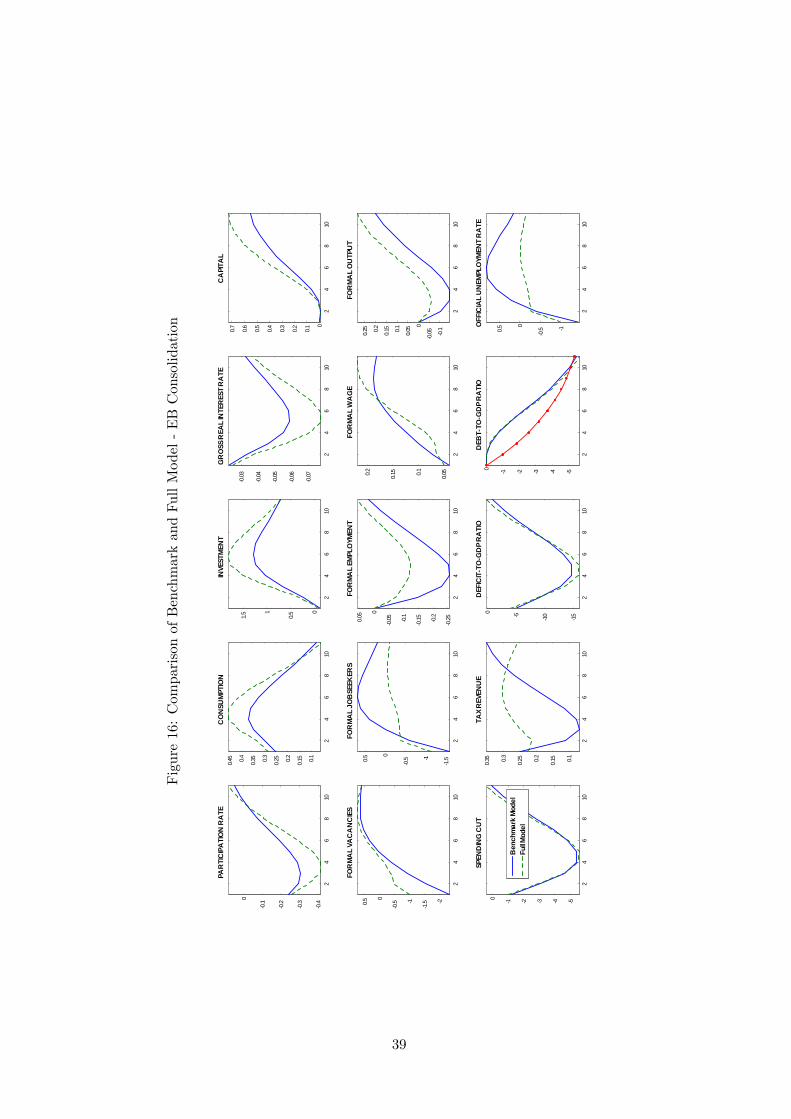
Figure16:ComparisonofBenchmarkandFullModel-EBConsolidation

24

68

10­0

.4

­0.3

­0.2

­0.1

0

PAR

TIC

IPA

TIO

N R

ATE

24

68

10

0.1

0.150.

2

0.250.

3

0.350.

4

0.45

CO

NSU

MPT

ION

24

68

10

0

0.51

1.5

INVE

STM

ENT

24

68

10

­0.0

7

­0.0

6

­0.0

5

­0.0

4

­0.0

3

GR

OSS

REA

L IN

TER

EST

RA

TE

24

68

100

0.1

0.2

0.3

0.4

0.5

0.6

0.7

CA

PITA

L

24

68

10

­2

­1.5­1

­0.5

0

0.5

FOR

MA

L VA

CA

NC

IES

24

68

10­1

.5­1

­0.5

0

0.5

FOR

MA

L JO

BSE

EKER

S

24

68

10­0

.25

­0.2

­0.1

5

­0.1

­0.0

5

0

0.05

FOR

MA

L EM

PLO

YMEN

T

24

68

10

0.050.

1

0.150.

2

FOR

MA

L W

AG

E

24

68

10

­0.1

­0.0

5

0

0.050.

1

0.150.

2

0.25

FOR

MA

L O

UTP

UT

24

68

10

­5­4­3­2­10

SPEN

DIN

G C

UT

24

68

10

0.1

0.150.

2

0.250.

3

0.35

TAX

REV

ENU

E

24

68

10

­15

­10­50

DEF

ICIT

­TO

­GD

P R

ATI

O

24

68

10

­5­4­3­2­10D

EBT­

TO­G

DP

RA

TIO

24

68

10

­1

­0.5

0

0.5O

FFIC

IAL

UN

EMPL

OYM

ENT

RA

TE

Ben

chm

ark

Mod

elFu

ll Mod

el

39

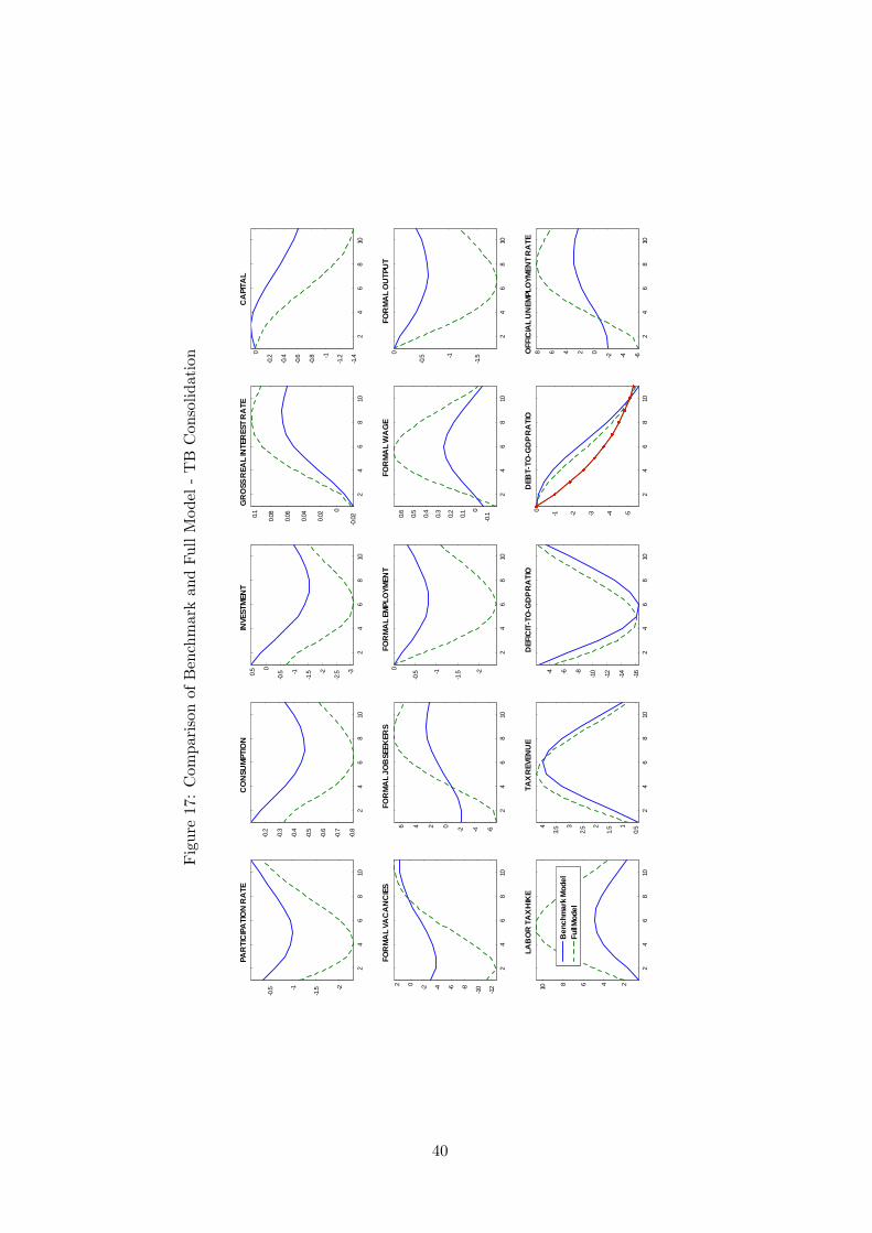
Figure17:ComparisonofBenchmarkandFullModel-TBConsolidation

24

68

10

­2

­1.5­1

­0.5

PAR

TIC

IPA

TIO

N R

ATE

24

68

10­0

.8

­0.7

­0.6

­0.5

­0.4

­0.3

­0.2

CO

NSU

MPT

ION

24

68

10­3

­2.5­2

­1.5­1

­0.5

0

0.5

INVE

STM

ENT

24

68

10­0

.02

0

0.02

0.04

0.06

0.080.

1

GR

OSS

REA

L IN

TER

EST

RA

TE

24

68

10­1

.4

­1.2­1

­0.8

­0.6

­0.4

­0.2

0

CA

PITA

L

24

68

10

­12

­10­8­6­4­202

FOR

MA

L VA

CA

NC

IES

24

68

10

­6­4­20246

FOR

MA

L JO

BSE

EKER

S

24

68

10

­2

­1.5­1

­0.5

0FO

RM

AL

EMPL

OYM

ENT

24

68

10

­0.1

0

0.1

0.2

0.3

0.4

0.5

0.6

FOR

MA

L W

AG

E

24

68

10

­1.5­1

­0.5

0FO

RM

AL

OU

TPU

T

24

68

10

246810

LAB

OR

TA

X H

IKE

24

68

100.

51

1.52

2.53

3.54

TAX

REV

ENU

E

24

68

10­1

6

­14

­12

­10­8­6­4

DEF

ICIT

­TO

­GD

P R

ATI

O

24

68

10

­5­4­3­2­10D

EBT­

TO­G

DP

RA

TIO

24

68

10­6­4­202468O

FFIC

IAL

UN

EMPL

OYM

ENT

RA

TE

Ben

chm

ark

Mod

elFu

ll Mod

el

40

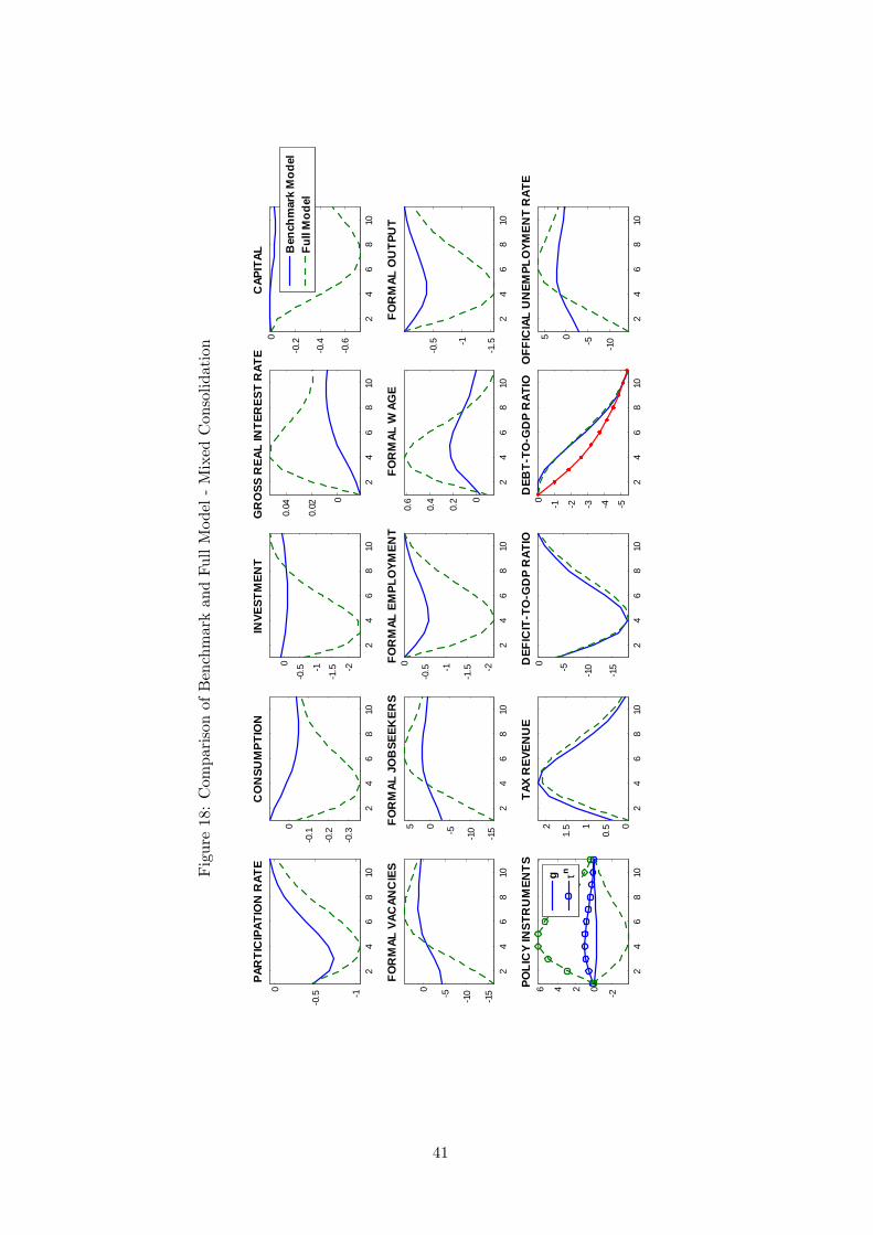
Figure18:ComparisonofBenchmarkandFullModel-MixedConsolidation

24

68

10­1

­0.5

0

PAR

TIC

IPAT

ION

RAT

E

24

68

10

­0.3

­0.2

­0.1

0

CO

NSU

MPT

ION

24

68

10

­2

­1.5­1

­0.5

0

INVE

STM

ENT

24

68

10

0

0.02

0.04

GR

OSS

REA

L IN

TER

EST

RAT

E

24

68

10

­0.6

­0.4

­0.2

0C

APIT

AL

24

68

10­1

5

­10­50

FOR

MAL

VAC

ANC

IES

24

68

10­1

5

­10­505FO

RM

AL J

OB

SEEK

ERS

24

68

10­2

­1.5­1

­0.5

0FOR

MAL

EM

PLO

YMEN

T

24

68

10

0

0.2

0.4

0.6

FOR

MAL

WAG

E

24

68

10­1

.5­1

­0.5

FOR

MAL

OU

TPU

T

24

68

10

­20246POLI

CY

INST

RU

MEN

TS

24

68

100

0.51

1.52

TAX

REV

ENU

E

24

68

10

­15

­10­50D

EFIC

IT­T

O­G

DP

RAT

IO

24

68

10

­5­4­3­2­10D

EBT­

TO­G

DP

RAT

IO

24

68

10

­10­505

OFF

ICIA

L U

NEM

PLO

YMEN

T R

ATE

g τn

Ben

chm

ark

Mod

elFu

ll M

odel

41

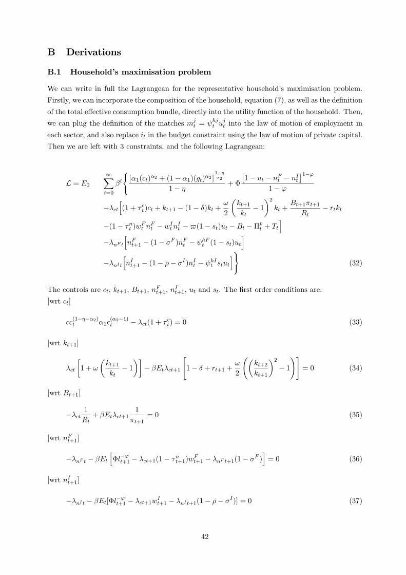
B Derivations

B.1 Household’s maximisation problem

We can write in full the Lagrangean for the representative household’s maximisation problem.

Firstly, we can incorporate the composition of the household, equation (7), as well as the definition

of the total effective consumption bundle, directly into the utility function of the household. Then,

we can plug the definition of the matches mjt = ψhjt u

jt into the law of motion of employment in

each sector, and also replace it in the budget constraint using the law of motion of private capital.

Then we are left with 3 constraints, and the following Lagrangean:

L = E0

∞∑t=0

βt

[α1(ct)

α2 + (1− α1)(gt)α2 ]

1−ηα2

1− η + Φ

[1− ut − nFt − nIt

]1−ϕ1− ϕ

−λct[(1 + τ ct)ct + kt+1 − (1− δ)kt +

ω

2

(kt+1

kt− 1

)2

kt +Bt+1πt+1

Rt− rtkt

−(1− τnt )wFt nFt − wIt nIt −$(1− st)ut −Bt −Πp

t + Tt

]−λnF t

[nFt+1 − (1− σF )nFt − ψhFt (1− st)ut

]−λnI t

[nIt+1 − (1− ρ− σI)nIt − ψhIt stut

](32)

The controls are ct, kt+1, Bt+1, nFt+1, nIt+1, ut and st. The first order conditions are:

[wrt ct]

cc(1−η−α2)t α1c

(α2−1)t − λct(1 + τ ct) = 0 (33)

[wrt kt+1]

λct

[1 + ω

(kt+1

kt− 1

)]− βEtλct+1

[1− δ + rt+1 +

ω

2

((kt+2

kt+1

)2

− 1

)]= 0 (34)

[wrt Bt+1]

−λct1

Rt+ βEtλct+1

1

πt+1= 0 (35)

[wrt nFt+1]

−λnF t − βEt[Φl−ϕt+1 − λct+1(1− τnt+1)wFt+1 − λnF t+1(1− σF )

]= 0 (36)

[wrt nIt+1]

−λnI t − βEt[Φl−ϕt+1 − λct+1w

It+1 − λnI t+1(1− ρ− σI)] = 0 (37)

42

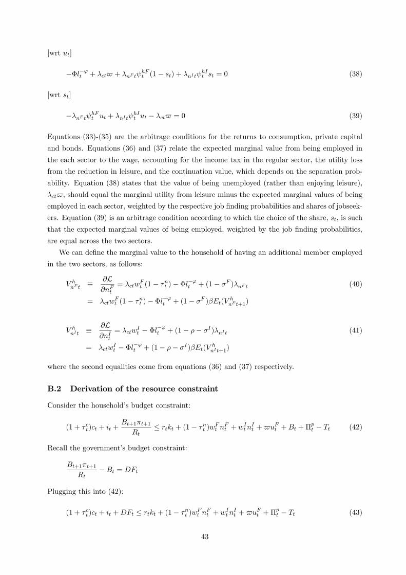
[wrt ut]

−Φl−ϕt + λct$ + λnF tψhFt (1− st) + λnI tψ

hIt st = 0 (38)

[wrt st]

−λnF tψhFt ut + λnI tψhIt ut − λct$ = 0 (39)

Equations (33)-(35) are the arbitrage conditions for the returns to consumption, private capital

and bonds. Equations (36) and (37) relate the expected marginal value from being employed in

the each sector to the wage, accounting for the income tax in the regular sector, the utility loss

from the reduction in leisure, and the continuation value, which depends on the separation prob-

ability. Equation (38) states that the value of being unemployed (rather than enjoying leisure),

λct$, should equal the marginal utility from leisure minus the expected marginal values of being

employed in each sector, weighted by the respective job finding probabilities and shares of jobseek-

ers. Equation (39) is an arbitrage condition according to which the choice of the share, st, is such

that the expected marginal values of being employed, weighted by the job finding probabilities,

are equal across the two sectors.

We can define the marginal value to the household of having an additional member employed

in the two sectors, as follows:

V hnF t ≡

∂L∂nFt

= λctwFt (1− τnt )− Φl−ϕt + (1− σF )λnF t (40)

= λctwFt (1− τnt )− Φl−ϕt + (1− σF )βEt(V

hnF t+1)

V hnI t ≡

∂L∂nIt

= λctwIt − Φl−ϕt + (1− ρ− σI)λnI t (41)

= λctwIt − Φl−ϕt + (1− ρ− σI)βEt(V h

nI t+1)

where the second equalities come from equations (36) and (37) respectively.

B.2 Derivation of the resource constraint

Consider the household’s budget constraint:

(1 + τ ct)ct + it +Bt+1πt+1

Rt≤ rtkt + (1− τnt )wFt n

Ft + wIt n

It +$uFt +Bt + Πp

t − Tt (42)

Recall the government’s budget constraint:

Bt+1πt+1

Rt−Bt = DFt

Plugging this into (42):

(1 + τ ct)ct + it +DFt ≤ rtkt + (1− τnt )wFt nFt + wIt n

It +$uFt + Πp

t − Tt (43)

43

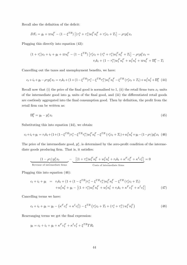
Recall also the definition of the deficit:

DFt = gt +$uFt − (1− ξTR)[(τnt + τ st )w

Ft n

Ft + τ ctct + Tt

]− ργpxt xt

Plugging this directly into equation (43):

(1 + τ ct)ct + it + gt +$uFt − (1− ξTR)[τ ctct + (τnt + τ st )w

Ft n

Ft + Tt

]− ργpxt xt =

rtkt + (1 − τnt )wFt nFt + wIt n

It + $uFt + Πp

t − Tt

Cancelling out the taxes and unemployment benefits, we have:

ct+ it+gt−ργpxt xt = rtkt+(1+(1−ξTR)τ st −ξTRτnt )wFt nFt −ξTR (τ ctct + Tt)+wIt n

It +Πp

t (44)

Recall now that (i) the price of the final good is normalised to 1, (ii) the retail firms turn xt units

of the intermediate good into yt units of the final good, and (iii) the differentiated retail goods

are costlessly aggregated into the final consumption good. Then by definition, the profit from the

retail firm can be written as:

Πpt = yt − pxt xt (45)

Substituting this into equation (44), we obtain:

ct+it+gt = rtkt+(1+(1−ξTR)τ st−ξTRτnt )wFt nFt −ξTR (τ ctct + Tt)+wIt n

It +yt−(1−ργ)pxt xt (46)

The price of the intermediate good, pxt , is determined by the zero-profit condition of the interme-

diate goods producing firm. That is, it satisfies:

(1− ργ) pxt xt︸ ︷︷ ︸Revenue of intermediate firms

−[(1 + τ st )w

Ft n

Ft + wIt n

It + rtkt + κFυFt + κIυIt

]︸ ︷︷ ︸Costs of intermediate firms

= 0

Plugging this into equation (46):

ct + it + gt = rtkt + (1 + (1− ξTR)τ st − ξTRτnt )wFt nFt − ξTR (τ ctct + Tt)

+wIt nIt + yt −

[(1 + τ st )w

Ft n

Ft + wIt n

It + rtkt + κFυFt + κIυIt

](47)

Cancelling terms we have:

ct + it + gt = yt −(κFυFt + κIυIt

)− ξTR

(τ ctct + Tt + (τ st + τnt )wFt n

Ft

)(48)

Rearranging terms we get the final expression:

yt = ct + it + gt + κFυFt + κIυIt + ξTRTRt

44

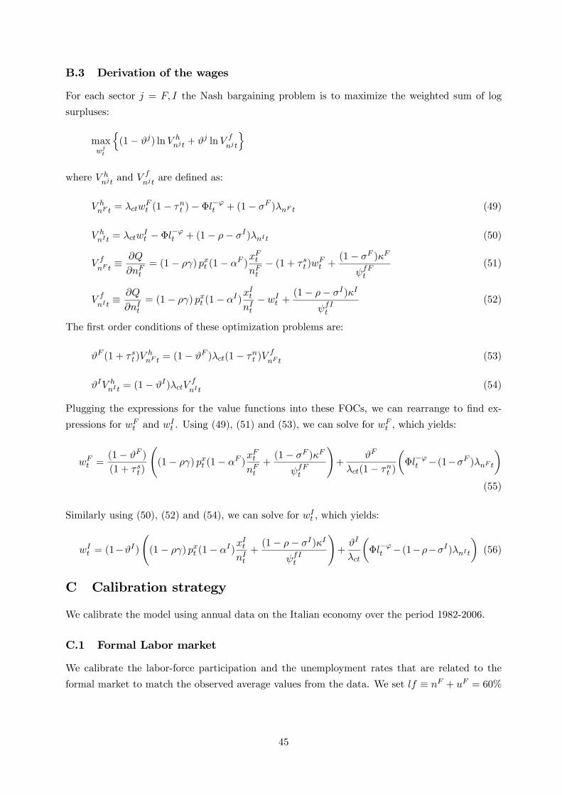
B.3 Derivation of the wages

For each sector j = F, I the Nash bargaining problem is to maximize the weighted sum of log

surpluses:

maxwjt

(1− ϑj) lnV h

njt + ϑj lnV fnjt

where V h

njtand V f

njtare defined as:

V hnF t = λctw

Ft (1− τnt )− Φl−ϕt + (1− σF )λnF t (49)

V hnI t = λctw

It − Φl−ϕt + (1− ρ− σI)λnI t (50)

V fnF t≡ ∂Q

∂nFt= (1− ργ) pxt (1− αF )

xFtnFt− (1 + τ st )w

Ft +

(1− σF )κF

ψfFt(51)

V fnI t≡ ∂Q

∂nIt= (1− ργ) pxt (1− αI)x

It

nIt− wIt +

(1− ρ− σI)κI

ψfIt(52)

The first order conditions of these optimization problems are:

ϑF (1 + τ st )VhnF t = (1− ϑF )λct(1− τnt )V f

nF t(53)

ϑIV hnI t = (1− ϑI)λctV f

nI t(54)

Plugging the expressions for the value functions into these FOCs, we can rearrange to find ex-

pressions for wFt and wIt . Using (49), (51) and (53), we can solve for w

Ft , which yields:

wFt =(1− ϑF )

(1 + τ st )

((1− ργ) pxt (1− αF )

xFtnFt

+(1− σF )κF

ψfFt

)+

ϑF

λct(1− τnt )

(Φl−ϕt −(1−σF )λnF t

)(55)

Similarly using (50), (52) and (54), we can solve for wIt , which yields:

wIt = (1−ϑI)(

(1− ργ) pxt (1− αI)xIt

nIt+

(1− ρ− σI)κI

ψfIt

)+ϑI

λct

(Φl−ϕt − (1−ρ−σI)λnI t

)(56)

C Calibration strategy

We calibrate the model using annual data on the Italian economy over the period 1982-2006.

C.1 Formal Labor market

We calibrate the labor-force participation and the unemployment rates that are related to the

formal market to match the observed average values from the data. We set lf ≡ nF + uF = 60%

45

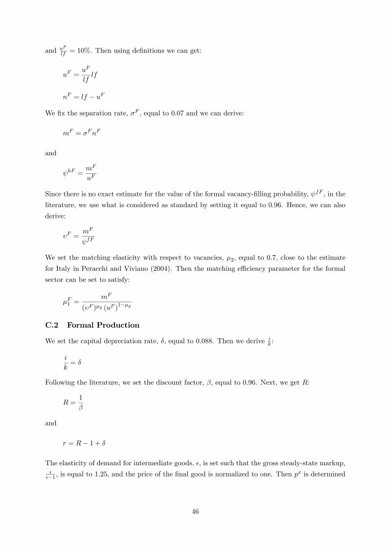
and uF

lf = 10%. Then using definitions we can get:

uF =uF

lflf

nF = lf − uF

We fix the separation rate, σF , equal to 0.07 and we can derive:

mF = σFnF

and

ψhF =mF

uF

Since there is no exact estimate for the value of the formal vacancy-filling probability, ψfF , in the

literature, we use what is considered as standard by setting it equal to 0.96. Hence, we can also

derive:

υF =mF

ψfF

We set the matching elasticity with respect to vacancies, µ2, equal to 0.7, close to the estimate

for Italy in Peracchi and Viviano (2004). Then the matching effi ciency parameter for the formal

sector can be set to satisfy:

µF1 =mF

(υF )µ2 (uF )1−µ2

C.2 Formal Production

We set the capital depreciation rate, δ, equal to 0.088. Then we derive ik :

i

k= δ

Following the literature, we set the discount factor, β, equal to 0.96. Next, we get R:

R =1

β

and

r = R− 1 + δ

The elasticity of demand for intermediate goods, ε, is set such that the gross steady-state markup,εε−1 , is equal to 1.25, and the price of the final good is normalized to one. Then px is determined

46

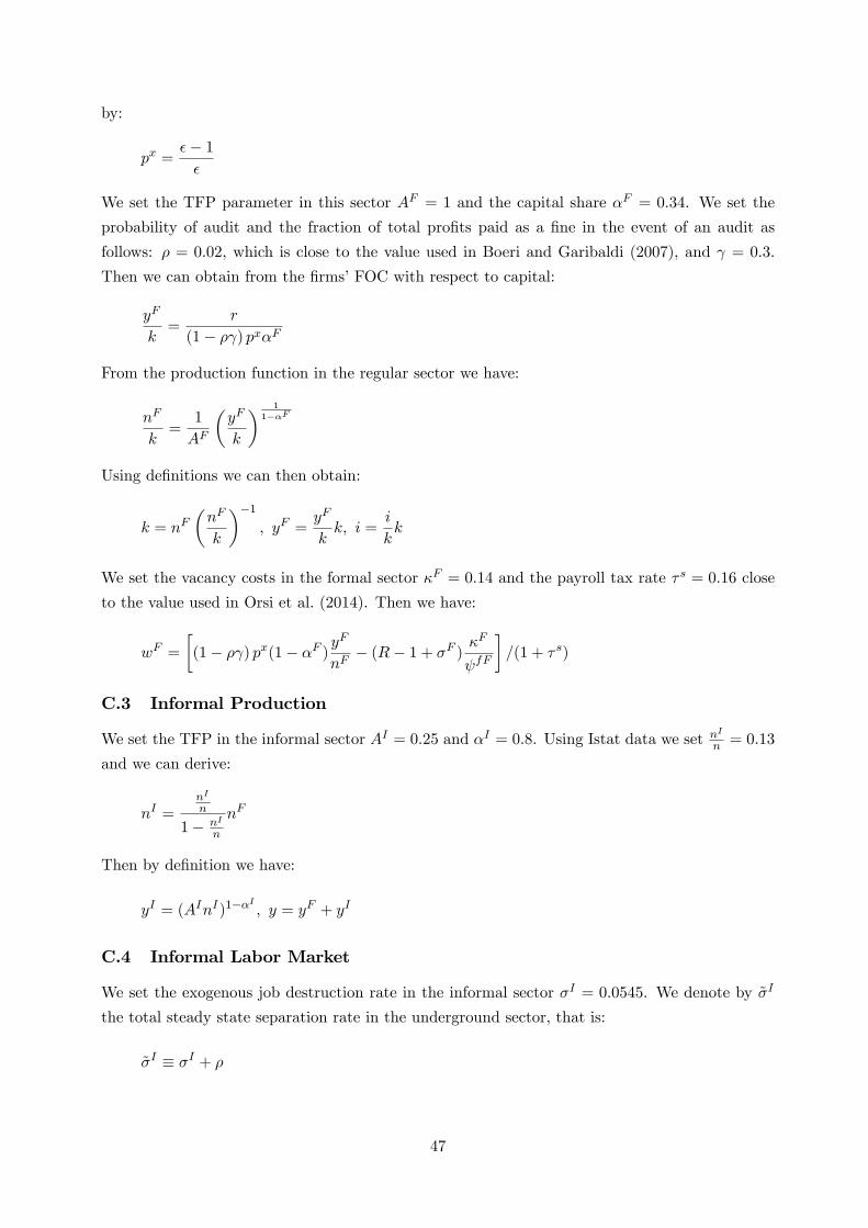
by:

px =ε− 1

ε

We set the TFP parameter in this sector AF = 1 and the capital share αF = 0.34. We set the

probability of audit and the fraction of total profits paid as a fine in the event of an audit as

follows: ρ = 0.02, which is close to the value used in Boeri and Garibaldi (2007), and γ = 0.3.

Then we can obtain from the firms’FOC with respect to capital:

yF

k=

r

(1− ργ) pxαF

From the production function in the regular sector we have:

nF

k=

1

AF

(yF

k

) 1

1−αF

Using definitions we can then obtain:

k = nF(nF

k

)−1

, yF =yF

kk, i =

i

kk

We set the vacancy costs in the formal sector κF = 0.14 and the payroll tax rate τ s = 0.16 close

to the value used in Orsi et al. (2014). Then we have:

wF =

[(1− ργ) px(1− αF )

yF

nF− (R− 1 + σF )

κF

ψfF

]/(1 + τ s)

C.3 Informal Production

We set the TFP in the informal sector AI = 0.25 and αI = 0.8. Using Istat data we set nI

n = 0.13

and we can derive:

nI =nI

n

1− nI

n

nF

Then by definition we have:

yI = (AInI)1−αI , y = yF + yI

C.4 Informal Labor Market

We set the exogenous job destruction rate in the informal sector σI = 0.0545. We denote by σI

the total steady state separation rate in the underground sector, that is:

σI ≡ σI + ρ

47

Then we have

mI = σInI

Then we set ψfI = 0.05 and get:

υI =mI

ψfI

We set the vacancy cost in the informal sector κI = 0.13 and derive

wI = (1− ργ) px(1− αI)yI

nI− (R− 1 + σI)

κI

ψfI

C.5 Fiscal Variables

Next, we set the replacement rate, $wF, equal to 0.35 close to the estimates in Martin (1996), also

used by Fugazza and Jacques (2004). Then by definition:

$ =$

wFwF

We set government spending and the tax rates as follows: gy = 11%, τn = 0.4, in line with Orsi et

al. (2014), and τ c = 0.18. Then by definition:

g =g

yy

We set the steady state debt-to-GDP ratio from the data, b = 103% and using the law of motion

of debt-to-GDP we derive

DF

y= (β − 1)b

and by definition

DF =DF

yy

We set the corruption parameter ξTR = 0.2. Then using the definition of the deficit we derive

TR =g +$uF − ργpxy −DF

1− ξTR

Then using the resource constraint we have:

c = y − i− g − κFυF − κIυI − ξTRTR

48

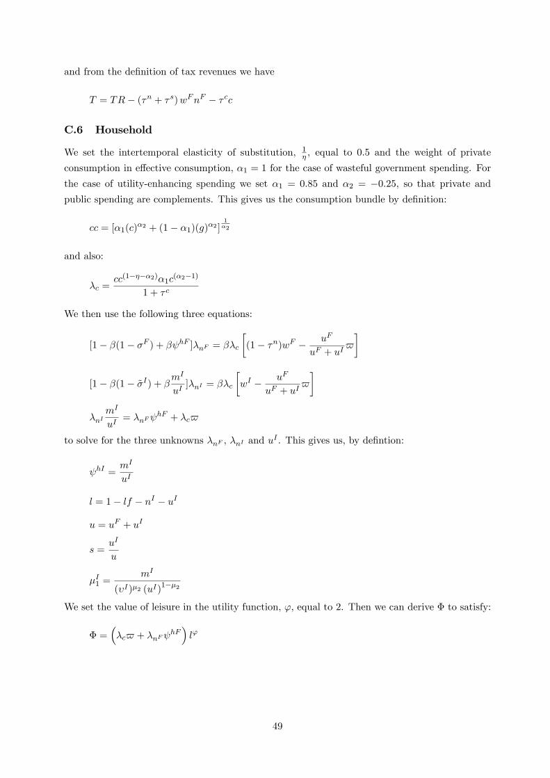
and from the definition of tax revenues we have

T = TR− (τn + τ s)wFnF − τ cc

C.6 Household

We set the intertemporal elasticity of substitution, 1η , equal to 0.5 and the weight of private

consumption in effective consumption, α1 = 1 for the case of wasteful government spending. For

the case of utility-enhancing spending we set α1 = 0.85 and α2 = −0.25, so that private and

public spending are complements. This gives us the consumption bundle by definition:

cc = [α1(c)α2 + (1− α1)(g)α2 ]1α2

and also:

λc =cc(1−η−α2)α1c

(α2−1)

1 + τ c

We then use the following three equations:

[1− β(1− σF ) + βψhF ]λnF = βλc

[(1− τn)wF − uF

uF + uI$

]

[1− β(1− σI) + βmI

uI]λnI = βλc

[wI − uF

uF + uI$

]

λnImI

uI= λnFψ

hF + λc$

to solve for the three unknowns λnF , λnI and uI . This gives us, by defintion:

ψhI =mI

uI

l = 1− lf − nI − uI

u = uF + uI

s =uI

u

µI1 =mI

(υI)µ2 (uI)1−µ2

We set the value of leisure in the utility function, ϕ, equal to 2. Then we can derive Φ to satisfy:

Φ =(λc$ + λnFψ

hF)lϕ

49

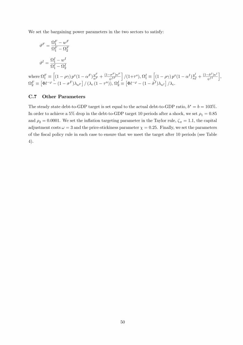
We set the bargaining power parameters in the two sectors to satisfy:

ϑF =ΩF

1 − wF

ΩF1 − ΩF

2

ϑI =ΩI

1 − wI

ΩI1 − ΩI

2

where ΩF1 ≡

[(1− ργ) px(1− αF ) y

F

nF+ (1−σF )κF

ψfF

]/(1+τ s), ΩI

1 ≡[(1− ργ) px(1− αI) y

I

nI + (1−σI)κI

ψfI

],

ΩF2 ≡

[Φl−ϕ − (1− σF )λnF

]/ (λc (1− τn)), ΩI

2 ≡[Φl−ϕ − (1− σI)λnI

]/λc.

C.7 Other Parameters

The steady state debt-to-GDP target is set equal to the actual debt-to-GDP ratio, b∗ = b = 103%.

In order to achieve a 5% drop in the debt-to-GDP target 10 periods after a shock, we set ρ1 = 0.85

and ρ2 = 0.0001. We set the inflation targeting parameter in the Taylor rule, ζπ = 1.1, the capital

adjustment costs ω = 3 and the price-stickiness parameter χ = 0.25. Finally, we set the parameters

of the fiscal policy rule in each case to ensure that we meet the target after 10 periods (see Table

4).

50