Fiscal Consolidation with Tax Evasion and Corruption

Evi Pappaa,1,∗, Rana Sajedia,2, Eugenia Vellaa,3

aEuropean University Institute, Florence, Italy, 50133

Abstract

Cross-country evidence highlights the importance of tax evasion and corruption in deter-

mining the size of fiscal multipliers. We introduce these two features in a New Keynesian

model and revisit the effects of fiscal consolidations. VAR evidence for Italy suggests that

spending cuts reduce tax evasion, while tax hikes increase it. In the model, spending cuts

induce a reallocation of production towards the formal sector, thus reducing tax evasion.

Tax hikes increase the incentives to produce in the less productive shadow sector, imply-

ing higher output and unemployment losses. Corruption further amplifies these losses by

requiring larger hikes in taxes to reduce debt. We use the model to assess the recent fiscal

consolidation plans in Greece, Italy, Portugal and Spain. Our results corroborate the evi-

dence of increasing levels of tax evasion during these consolidations and point to significant

output and welfare losses, which could be reduced substantially by combating tax evasion

and corruption.

1. Introduction

When there is an income tax, the just man will pay more and the unjust less on the

same amount of income. Plato, The Republic, Book I, 343-D

The recent fiscal crisis has sparked a considerable amount of research measuring the

macroeconomic effects of fiscal consolidations.4 This literature, however, has left aside two

crucial political economy aspects, namely the presence of tax evasion and corruption. This

is surprising, given that they are important features in many of the countries adopting

consolidation policies, as seen in Figure 1. In addition, there is growing evidence that tax

evasion and corruption have increased in recent years. For example, a recent report by the

technical staff of the Spanish Finance Ministry (Gestha, 2014) indicates that the shadow

economy in Spain increased by 6.8 percentage points between 2008 and 2012, reaching

24.6% of GDP. At the same time, a special Greek police task force reported in 2013 that

∗Corresponding author1Email address: evi.pappa@eui.eu, Telephone number: +39 055 46859082Email address: rana.sajedi@eui.eu3Email address: eugenia.vella@eui.eu4The implementation of the Maastricht Treaty in the mid 1990s initiated a wave of research on the

effects of consolidations. For examples, see the survey in Perotti (1996).

Preprint submitted to Elsevier December 11, 2014

the number of cases of public corruption increased by 33% between 2011 and 2012.5 The

aim of this paper is to revisit the effects of government expenditure cuts and labor tax

hikes on output, unemployment and welfare, when tax evasion and corruption are present.

We treat tax evasion as synonymous with the shadow economy, which, according to

Buehn and Schneider (2012, p.175-176), comprises “all market-based, lawful production or

trade of goods and services deliberately concealed from public authorities in order to evade

either payment of income, value added or other taxes, or social security contributions”.

Fiscal policy has an impact on the size of the shadow economy since it affects the incentives

to tax evade both directly, through the tax burden, and indirectly, through its effects on

the formal economy. Thus, a fiscal consolidation can have important secondary effects if it

generates a reallocation of resources between the formal and informal sectors.6 Corruption,

in our paper, refers to the embezzlement of public funds. The presence of corruption can

hamper the ability of the government to raise revenue, and thus distort the effects of

fiscal consolidations. Tax evasion and corruption often coexist and possibly interact. For

instance, Buehn and Schneider (2012) indicate that there is a positive correlation between

the two.

Many authors have studied whether it is preferable to rely on spending cuts or tax

hikes when consolidating the public deficit. Overall, the findings are not conclusive. Using

multi-year fiscal consolidation data for 17 OECD countries over the period 1980-2005,

Alesina et al. (2013) show that expenditure-based adjustments are typically associated

with mild and short-lived recessions, and in some cases with no recession at all, while tax-

based corrections are followed by deep and prolonged recessions. On the other hand, Erceg

and Linde (2013) reach a different conclusion. Using a two-country Dynamic Stochastic

General Equilibrium (DSGE) model of a currency union, they show that, in the short run,

a spending cut depresses output by more than a labor tax hike, because of the limited

accommodation by the central bank and the fixed exchange rate. However, this is reversed

in the long run as real interest and exchange rates adjust towards their flexible price levels.

Indeed, there is strong evidence that the effects of fiscal consolidations are not yet fully

understood. Blanchard and Leigh (2013) examine the impact of the recent fiscal consoli-

dations in 26 OECD countries. They regress the forecast errors of output growth between

2010-2011 on the planned consolidation of public deficit, and find that the forecasts under-

estimate the size of fiscal multipliers. As shown in the next section, the underestimation of

fiscal multipliers is more pronounced in countries with a higher level of tax evasion and/or

corruption, suggesting that these two features amplify the effects of fiscal consolidations.

Reliable time series data on tax evasion is typically hard to get. Luckily, the Italian

5See http://greece.greekreporter.com/2013/04/02/greek-police-public-worker-corruption-soars/6For example, using a model calibrated to firm-level data for Greece, Pappada and Zylberberg (2014)

show that the increase in tax evasion can explain three quarters of the revenue leakages following the 2010VAT hikes, when only half of the expected increase in revenue was realized. Colombo et al. (2014) alsoshow empirical evidence of a rise in the shadow economy in recent years, although their focus is on the roleof the banking crisis.

2

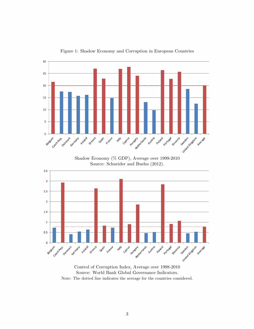
Figure 1: Shadow Economy and Corruption in European Countries

Shadow Economy (% GDP), Average over 1999-2010Source: Schneider and Buehn (2012).

Control of Corruption Index, Average over 1998-2010Source: World Bank Global Governance Indicators.

Note: The dotted line indicates the average for the countries considered.

3

National Institute of Statistics (ISTAT) has created and regularly updated a time series

of informal employment in Italy, which is consistent with international standards and,

in particular, with the 1993 System of National Accounts. Apart from data availability,

Italy is a fitting case for studying tax evasion and corruption. Firstly, there is abundant

evidence of a large shadow economy, with estimates varying between 15% and 30% of GDP

(see e.g. Ardizzi et al., 2012, Orsi et al., 2014, and Schneider and Buehn, 2012). Secondly,

Busato and Chiarini (2004) have shown that incorporating the shadow economy in an

RBC model for Italy considerably improves the fit to the data. Thirdly, Italy scores poorly

in international rankings of institutional quality: it is currently ranked 72nd among 176

countries with a score of 42/100 in Transparency International’s Corruption Perception

Index and 25th among the 27 EU members in the index for the ‘Quality of Government’

(see Charron et al., 2012).7

In the first part of this paper, we incorporate the ISTAT series on informal employ-

ment in a VAR, and identify the effects of fiscal consolidations occurring through a fall

in government consumption expenditure or an increase in direct taxes. We find that both

types of shocks are contractionary, both reducing output and increasing unemployment.

However, tax hikes significantly increase informal employment, while spending cuts reduce

it.

To understand the mechanisms driving the results, we reassess the effects of fiscal

consolidations in a model with price stickiness, search and matching frictions, endogenous

labor force participation, tax evasion and corruption. The economy features a regular

and an informal sector, and the transactions in the latter sector are not recorded by the

government. Firms can hire informal labor to hide part of their production and evade

payroll taxes. Households may also evade personal income taxation by reallocating their

labor to the informal sector. In each period, there is a positive probability that irregular

employment is detected, in which case the worker loses the job and the firm pays a fine.

Corruption implies that a fraction of tax revenues is embezzled. Following Erceg and

Linde (2013), either labor tax rates or government consumption expenditures react to the

deviation of the debt-to-GDP ratio from a target value. Fiscal consolidation occurs when

this target is hit by a negative shock.

We find that the presence of tax evasion and corruption amplifies the negative effects

of labor tax hikes on output and unemployment, while it mitigates those of expenditure

cuts. Tax evasion and corruption imply that a larger increase in the tax rate is needed to

reduce debt, and this amplifies the distortionary effects of the consolidation. Tax evasion

further increases the output losses after a tax hike because workers and firms reallocate

resources to the informal sector, increasing inefficiencies since this sector is less productive.

On the other hand, government spending cuts reduce tax evasion. The spending cut

7The Corruption Perception Index is based on a cross-country survey assessing the degree of transparencyin public administration. The ‘Quality of Government’ index accounts for other pillars, such as protectionof the rule of law, government effectiveness and accountability, in addition to corruption.

4

creates a positive wealth effect which increases consumption and investment and reduces

labor force participation. Agents reallocate their labor search towards the formal sector,

first because it is more productive, and second because the formal labor market has a

higher matching efficiency and a lower job destruction rate. Hence, the share of shadow

employment in total employment is reduced. Relative to standard models, tax evasion

and corruption increase the size of this wealth effect, thereby increasing the crowding-in of

private consumption, and reducing output losses.

Labor tax hikes are costly in terms of welfare, but spending cuts typically involve

welfare gains, since private consumption increases and labor supply decreases. The latter

result is reversed, however, if government spending directly enters the utility of households,

or if agents are liquidity constrained.

We use our model to compare the recent consolidation policies in Greece, Italy, Spain

and Portugal, all countries that are characterized by both high corruption and tax evasion.

Despite the fact that the consolidation plans rely heavily on spending cuts, the model

predicts increasing levels of tax evasion in all countries, as well as prolonged recessions.

The largest output losses are observed in Portugal, due to the size of the tax hikes, and

Greece, due to the severity of the austerity measures. There are also substantial welfare

losses in all countries; the largest occurs in Portugal because of the significant tax hikes in

the consolidation package.

There have been considerable discussions in the policy arena about combating both

tax evasion and corruption. For example, members of the European Parliament organized

an event focusing on corruption and tax evasion in Ljubljana in May 2013. The issue of

reducing tax evasion also dominated the 2013 meeting of G8 leaders. To quantitatively

evaluate the welfare gains from fighting tax evasion and corruption, we perform a coun-

terfactual analysis of the consolidation plans when we reduce the degree of corruption and

tax evasion. We find that both battles are worth fighting as they significantly reduce the

welfare losses from fiscal consolidation.

The remainder of the paper is organized as follows. In the next section we present

empirical evidence to motivate our work. In Section 3 we develop the model and its

calibration. Section 4 discusses the main theoretical results. Section 5 presents the policy

comparisons and Section 6 concludes.

2. Empirical Evidence

This section is divided into two parts. We first present evidence highlighting the impor-

tance of corruption and tax evasion in determining the size of fiscal multipliers. Here, we

extend the cross-country regressions of Blanchard and Leigh (2013), henceforth BL (2013),

controlling for tax evasion and public corruption, and we check the robustness of our con-

clusions by considering the output effects of narrative consolidation shocks. We then use

the ISTAT data on shadow employment to run VAR regressions examining the effects of

spending cuts and tax hikes on output, unemployment and shadow employment in Italy.

5

2.1. Do Tax Evasion and Corruption Matter?

To motivate our study, we replicate the BL (2013) regressions, controlling for tax evasion

and public corruption. As a proxy for tax evasion we use the estimates of the share of

shadow output to total GDP provided by Elgin and Oztunalı (2012), while for corruption

we use the Corruption Perception Index. We group the 26 European countries considered

by BL (2013) into either high and low tax evasion, or high and low corruption.8 We then

add to the BL (2013) regressions a dummy which is equal to one for the high corruption

or tax evasion group. We also run the same regression using a dummy for both high

corruption and tax evasion; in this case we drop three countries which do not fall into the

same group across the two indices.9

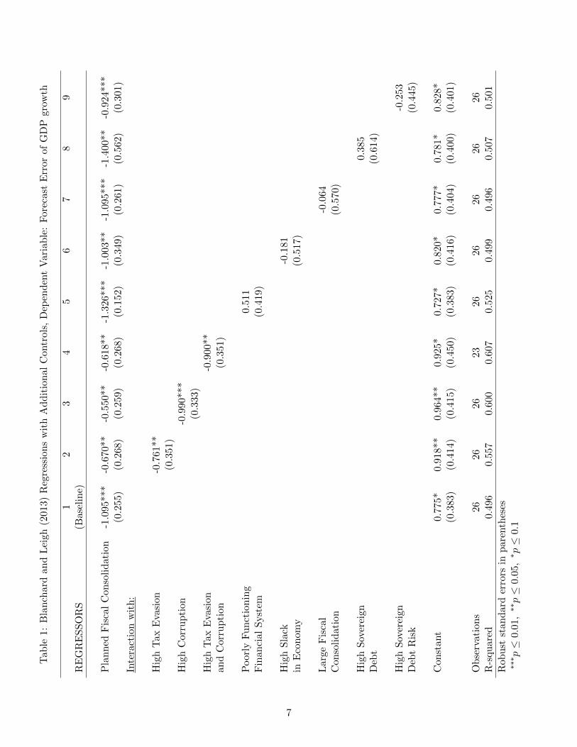
The results are shown in Table 1. The first column replicates the findings of BL (2013).

The planned fiscal consolidation variable is significant at 1% and has a coefficient of -1.095,

implying that “for every additional percentage point of fiscal consolidation as a percentage

of GDP, output was 1 percent lower than forecast” (BL, 2013, p.8). Thus, fiscal multipliers

are underestimated. Columns 2 to 4 show the results when we include the interaction of the

planned fiscal consolidation variable with our dummies for high tax evasion and corruption.

While the coefficient is still significant at 5% when the dummy variables are included, it

is lower in absolute value. On the other hand, the interaction term is always significant,

showing that there is a significant difference in the coefficients between the two groups.

Our estimates imply that the coefficient on the planned fiscal consolidation is -1.431 for

the high tax evasion group, -1.540 for the high corruption group, and -1.518 for the high

tax evasion and corruption group. In all cases, they are larger, in absolute value, than

the baseline results of BL (2013), indicating that the implicit underestimation of fiscal

multipliers is more pronounced in countries with higher tax evasion and/or corruption. In

other words, these two features amplify the effects of fiscal consolidations.

The BL (2013) methodology has been criticized in a number of ways. Of particular

importance for our study is the fact that the regression may not truly capture the effect of

fiscal multipliers on forecast errors. Given that the forecasts are conditional not only on

fiscal shocks but on the full set of information used by the forecaster, forecast errors may

depend on factors other than underestimated fiscal multipliers.

8We use a two-mean clustering algorithm to endogenously group the countries. The resulting ‘hightax evasion’ group comprises Belgium, Bulgaria, Cyprus, Greece, Hungary, Italy, Malta, Poland, Portugal,Romania, Slovenia and Spain, while the ‘low tax evasion’ group includes Austria, Czech Republic, Denmark,Finland, France, Germany, Iceland, Ireland, Netherlands, Norway, Sweden, Switzerland, Slovakia and theUK. The ‘high corruption’ group comprises Bulgaria, Cyprus, Czech Republic, Greece, Hungary, Italy,Malta, Poland, Portugal, Romania, Slovakia, Slovenia and Spain, while the ‘low corruption’ group includesAustria, Belgium, Denmark, Finland, France, Germany, Iceland, Ireland, Netherlands, Norway, Sweden,Switzerland, and the UK.

9An alternative way of carrying out this analysis would be to include the indices as controls in theregression. We have chosen to use the dummy variable approach because, although we have robust groupingsof countries in terms of high and low tax evasion and corruption, there is not enough cross-sectional variationin either index to add them directly in the regression, and also to avoid issues of generated regressor bias,since both measures are estimates of the underlying variables of interest.

6

Tab

le1:

Bla

nch

ard

and

Lei

gh(2

013

)R

egre

ssio

ns

wit

hA

dd

itio

nal

Con

trol

s,D

epen

den

tV

aria

ble

:F

orec

ast

Err

orof

GD

Pgr

owth

12

34

56

78

9R

EG

RE

SS

OR

S(B

ase

lin

e)

Pla

nn

edF

isca

lC

on

soli

dati

on-1

.095

***

-0.6

70**

-0.5

50**

-0.6

18**

-1.3

26**

*-1

.003

**-1

.095

***

-1.4

00**

-0.9

24**

*(0

.255)

(0.2

68)

(0.2

59)

(0.2

68)

(0.1

52)

(0.3

49)

(0.2

61)

(0.5

62)

(0.3

01)

Inte

ract

ion

wit

h:

Hig

hT

ax

Eva

sion

-0.7

61**

(0.3

51)

Hig

hC

orru

pti

on-0

.990

***

(0.3

33)

Hig

hT

ax

Eva

sion

-0.9

00**

and

Cor

rup

tion

(0.3

51)

Poorl

yF

un

ctio

nin

g0.

511

Fin

an

cial

Syst

em(0

.419

)

Hig

hS

lack

-0.1

81in

Eco

nom

y(0

.517

)

Larg

eF

isca

l-0

.064

Con

soli

dat

ion

(0.5

70)

Hig

hS

over

eign

0.38

5D

ebt

(0.6

14)

Hig

hS

over

eign

-0.2

53D

ebt

Ris

k(0

.445

)

Con

stan

t0.7

75*

0.91

8**

0.96

4**

0.92

5*0.

727*

0.82

0*0.

777*

0.78

1*0.

828*

(0.3

83)

(0.4

14)

(0.4

15)

(0.4

50)

(0.3

83)

(0.4

16)

(0.4

04)

(0.4

00)

(0.4

01)

Ob

serv

ati

on

s26

2626

2326

2626

2626

R-s

qu

are

d0.

496

0.55

70.

600

0.60

70.

525

0.49

90.

496

0.50

70.

501

Rob

ust

stan

dar

der

rors

inp

aren

thes

es∗∗∗ p≤

0.0

1,∗∗p≤

0.05,∗ p≤

0.1

7

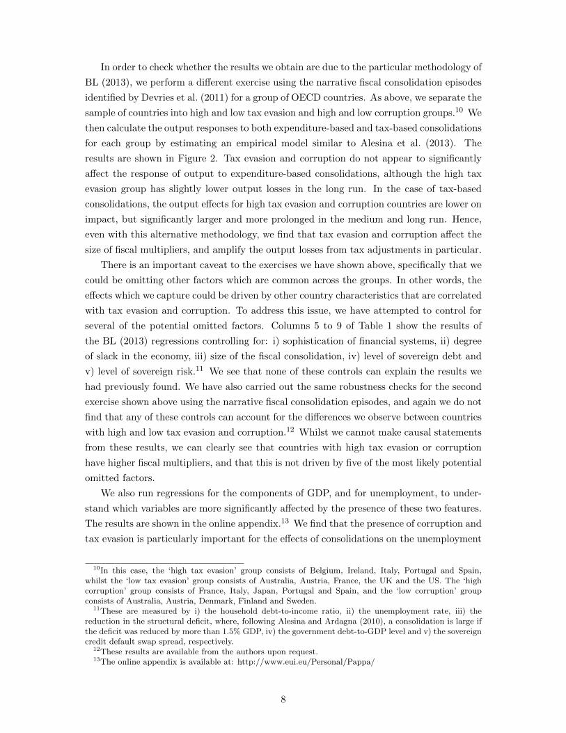
In order to check whether the results we obtain are due to the particular methodology of

BL (2013), we perform a different exercise using the narrative fiscal consolidation episodes

identified by Devries et al. (2011) for a group of OECD countries. As above, we separate the

sample of countries into high and low tax evasion and high and low corruption groups.10 We

then calculate the output responses to both expenditure-based and tax-based consolidations

for each group by estimating an empirical model similar to Alesina et al. (2013). The

results are shown in Figure 2. Tax evasion and corruption do not appear to significantly

affect the response of output to expenditure-based consolidations, although the high tax

evasion group has slightly lower output losses in the long run. In the case of tax-based

consolidations, the output effects for high tax evasion and corruption countries are lower on

impact, but significantly larger and more prolonged in the medium and long run. Hence,

even with this alternative methodology, we find that tax evasion and corruption affect the

size of fiscal multipliers, and amplify the output losses from tax adjustments in particular.

There is an important caveat to the exercises we have shown above, specifically that we

could be omitting other factors which are common across the groups. In other words, the

effects which we capture could be driven by other country characteristics that are correlated

with tax evasion and corruption. To address this issue, we have attempted to control for

several of the potential omitted factors. Columns 5 to 9 of Table 1 show the results of

the BL (2013) regressions controlling for: i) sophistication of financial systems, ii) degree

of slack in the economy, iii) size of the fiscal consolidation, iv) level of sovereign debt and

v) level of sovereign risk.11 We see that none of these controls can explain the results we

had previously found. We have also carried out the same robustness checks for the second

exercise shown above using the narrative fiscal consolidation episodes, and again we do not

find that any of these controls can account for the differences we observe between countries

with high and low tax evasion and corruption.12 Whilst we cannot make causal statements

from these results, we can clearly see that countries with high tax evasion or corruption

have higher fiscal multipliers, and that this is not driven by five of the most likely potential

omitted factors.

We also run regressions for the components of GDP, and for unemployment, to under-

stand which variables are more significantly affected by the presence of these two features.

The results are shown in the online appendix.13 We find that the presence of corruption and

tax evasion is particularly important for the effects of consolidations on the unemployment

10In this case, the ‘high tax evasion’ group consists of Belgium, Ireland, Italy, Portugal and Spain,whilst the ‘low tax evasion’ group consists of Australia, Austria, France, the UK and the US. The ‘highcorruption’ group consists of France, Italy, Japan, Portugal and Spain, and the ‘low corruption’ groupconsists of Australia, Austria, Denmark, Finland and Sweden.

11These are measured by i) the household debt-to-income ratio, ii) the unemployment rate, iii) thereduction in the structural deficit, where, following Alesina and Ardagna (2010), a consolidation is large ifthe deficit was reduced by more than 1.5% GDP, iv) the government debt-to-GDP level and v) the sovereigncredit default swap spread, respectively.

12These results are available from the authors upon request.13The online appendix is available at: http://www.eui.eu/Personal/Pappa/

8

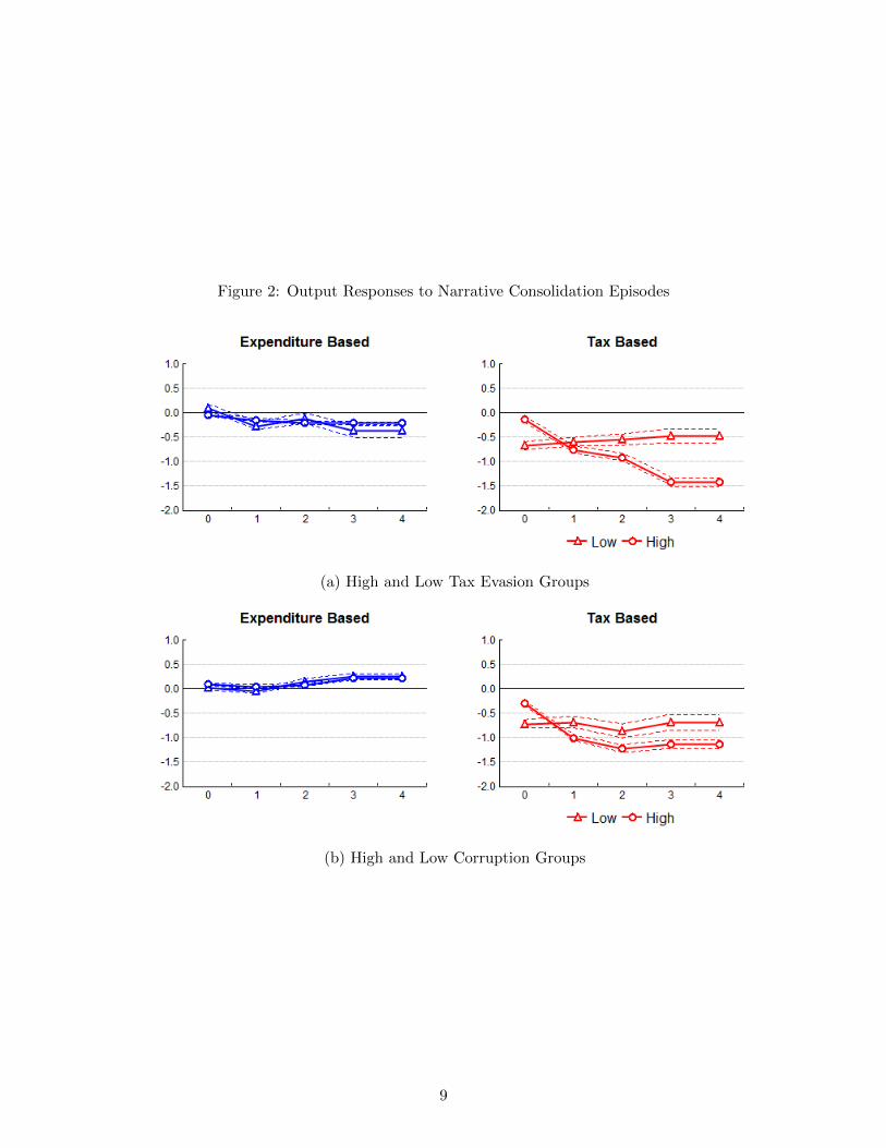
Figure 2: Output Responses to Narrative Consolidation Episodes

(a) High and Low Tax Evasion Groups

(b) High and Low Corruption Groups

9

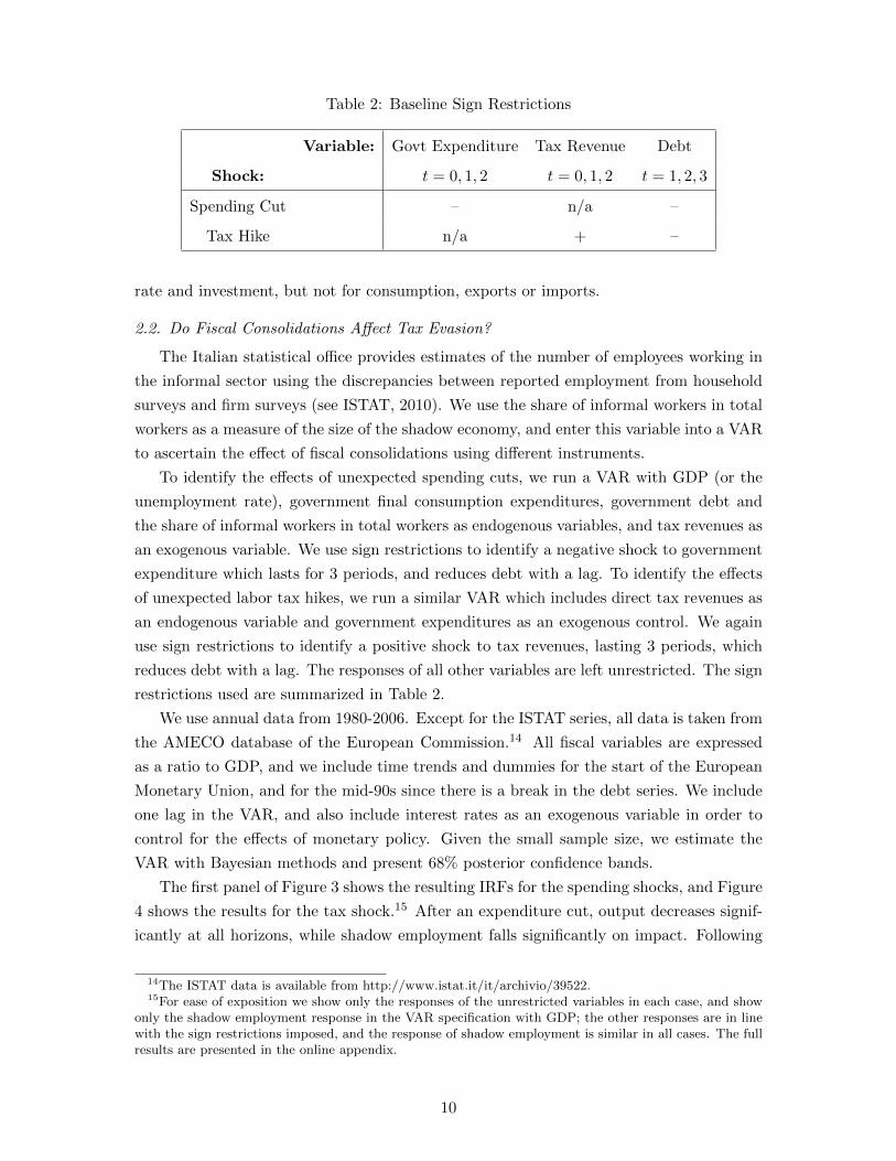
Table 2: Baseline Sign Restrictions

Variable: Govt Expenditure Tax Revenue Debt

Shock: t = 0, 1, 2 t = 0, 1, 2 t = 1, 2, 3

Spending Cut – n/a –

Tax Hike n/a + –

rate and investment, but not for consumption, exports or imports.

2.2. Do Fiscal Consolidations Affect Tax Evasion?

The Italian statistical office provides estimates of the number of employees working in

the informal sector using the discrepancies between reported employment from household

surveys and firm surveys (see ISTAT, 2010). We use the share of informal workers in total

workers as a measure of the size of the shadow economy, and enter this variable into a VAR

to ascertain the effect of fiscal consolidations using different instruments.

To identify the effects of unexpected spending cuts, we run a VAR with GDP (or the

unemployment rate), government final consumption expenditures, government debt and

the share of informal workers in total workers as endogenous variables, and tax revenues as

an exogenous variable. We use sign restrictions to identify a negative shock to government

expenditure which lasts for 3 periods, and reduces debt with a lag. To identify the effects

of unexpected labor tax hikes, we run a similar VAR which includes direct tax revenues as

an endogenous variable and government expenditures as an exogenous control. We again

use sign restrictions to identify a positive shock to tax revenues, lasting 3 periods, which

reduces debt with a lag. The responses of all other variables are left unrestricted. The sign

restrictions used are summarized in Table 2.

We use annual data from 1980-2006. Except for the ISTAT series, all data is taken from

the AMECO database of the European Commission.14 All fiscal variables are expressed

as a ratio to GDP, and we include time trends and dummies for the start of the European

Monetary Union, and for the mid-90s since there is a break in the debt series. We include

one lag in the VAR, and also include interest rates as an exogenous variable in order to

control for the effects of monetary policy. Given the small sample size, we estimate the

VAR with Bayesian methods and present 68% posterior confidence bands.

The first panel of Figure 3 shows the resulting IRFs for the spending shocks, and Figure

4 shows the results for the tax shock.15 After an expenditure cut, output decreases signif-

icantly at all horizons, while shadow employment falls significantly on impact. Following

14The ISTAT data is available from http://www.istat.it/it/archivio/39522.15For ease of exposition we show only the responses of the unrestricted variables in each case, and show

only the shadow employment response in the VAR specification with GDP; the other responses are in linewith the sign restrictions imposed, and the response of shadow employment is similar in all cases. The fullresults are presented in the online appendix.

10

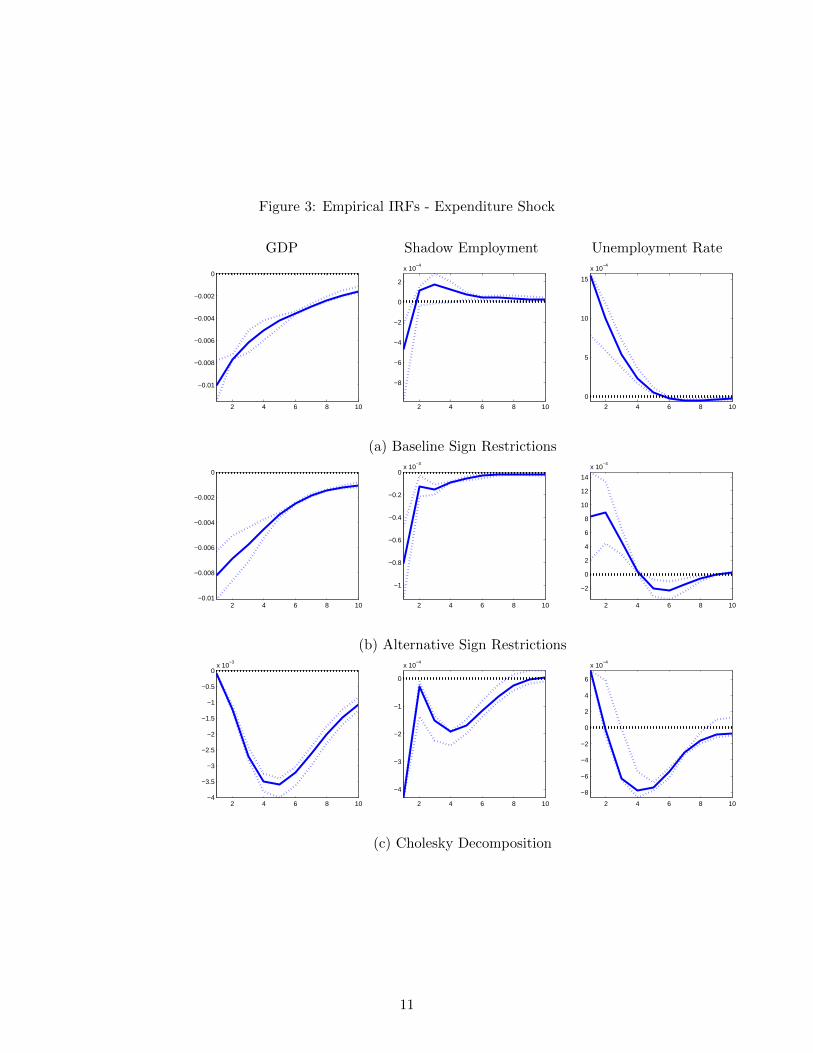
Figure 3: Empirical IRFs - Expenditure Shock

GDP Shadow Employment Unemployment Rate

2 4 6 8 10

−0.01

−0.008

−0.006

−0.004

−0.002

0

2 4 6 8 10

−8

−6

−4

−2

0

2

x 10−4

2 4 6 8 10

0

5

10

15

x 10−4

(a) Baseline Sign Restrictions

2 4 6 8 10−0.01

−0.008

−0.006

−0.004

−0.002

0

2 4 6 8 10

−1

−0.8

−0.6

−0.4

−0.2

0x 10

−3

2 4 6 8 10

−2

0

2

4

6

8

10

12

14

x 10−4

(b) Alternative Sign Restrictions

2 4 6 8 10−4

−3.5

−3

−2.5

−2

−1.5

−1

−0.5

0x 10

−3

2 4 6 8 10

−4

−3

−2

−1

0

x 10−4

2 4 6 8 10

−8

−6

−4

−2

0

2

4

6

x 10−4

(c) Cholesky Decomposition

11

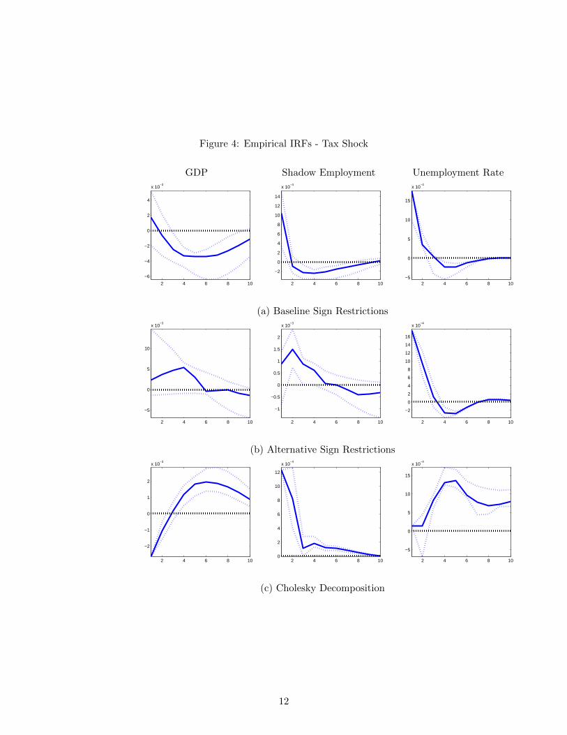
Figure 4: Empirical IRFs - Tax Shock

GDP Shadow Employment Unemployment Rate

2 4 6 8 10

−6

−4

−2

0

2

4

x 10−3

2 4 6 8 10

−2

0

2

4

6

8

10

12

14

x 10−4

2 4 6 8 10−5

0

5

10

15

x 10−4

(a) Baseline Sign Restrictions

2 4 6 8 10

−5

0

5

10

x 10−3

2 4 6 8 10

−1

−0.5

0

0.5

1

1.5

2

x 10−3

2 4 6 8 10

−2

0

2

4

6

8

10

12

14

16

x 10−4

(b) Alternative Sign Restrictions

2 4 6 8 10

−2

−1

0

1

2

x 10−3

2 4 6 8 100

2

4

6

8

10

12

x 10−4

2 4 6 8 10

−5

0

5

10

15

x 10−4

(c) Cholesky Decomposition

12

a tax hike, output does not fall on impact but the response is significantly negative in the

medium run, and there is a significant rise in shadow employment on impact. When the

unemployment rate is used instead of output, we see that it rises significantly after both

types of consolidation.

The correct identification of fiscal shocks is highly contested in the literature, and there

are justifiable concerns regarding the robustness of VAR results to different identification

schemes. To demonstrate the robustness of our qualitative results, we examine their sen-

sitivity to alternative identification schemes. The second panel of Figures 3 and 4 present

responses when we use an alternative set of sign restrictions in which we jointly identify

spending cuts and tax hikes in the same VAR regression, by assuming that they are un-

correlated. The final panel presents results when we use a simple Cholesky decomposition

to identify the shocks, ordering government spending and tax revenues first in the system.

Whilst the precise pattern of the responses can differ, the result broadly remains that con-

solidations are contractionary, and that spending-based consolidations reduce tax evasion

whilst tax-based consolidations increase it. Since the zero restrictions imposed in both the

alternative sign restrictions and the Cholesky are unlikely to hold in annual data, and we

are restricted to using annual data due to the availability of data on shadow employment,

we feel that our baseline sign restrictions are the most valid choice.16

Another potential problem with the SVAR methodology is whether the shocks we have

identified can be anticipated. Dealing comprehensively with this issue is not straightfor-

ward, and is beyond the scope of this paper. As a first pass at ascertaining whether the

shocks we have identified are truly unanticipated, we follow Perotti (2005) and regress

the spending shocks, identified in our baseline sign restrictions, on forecast errors from

professional forecasts of government expenditure, taken from the ECB’s survey of profes-

sional forecasts. The first column of Table 3 shows the results from regressions using the

“raw” forecast errors, and the second column shows the results using the residuals after

regressing the forecast errors on the lag of the 4 variables in the VAR. We see that in both

cases, the forecast errors are uncorrelated to our shocks, suggesting that our shocks are

not predictable.

Thus the data robustly suggests that fiscal consolidation through expenditure cuts

leads to a fall in shadow employment, while a consolidation through tax hikes increases

shadow employment, and that both types of consolidations are contractionary. In the next

section we develop a model with tax evasion and corruption to replicate these findings and

understand how these frictions affect the propagation of fiscal shocks.

16We have also used the narrative fiscal consolidation episodes identified by Devries et al. (2011), however,given that they provide very few episodes for Italy alone, we do not find significant responses. Further detailsof all these exercises are provided in the online appendix.

13

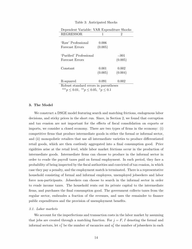
Table 3: Anticipated Shocks

Dependent Variable: VAR Expenditure Shocks

REGRESSOR 1 2

‘Raw’ Professional 0.006Forecast Errors (0.005)

‘Purified’ Professional -.001Forecast Errors (0.005)

Constant 0.001 0.002(0.005) (0.004)

R-squared 0.091 0.002

Robust standard errors in parentheses∗∗∗p ≤ 0.01, ∗∗p ≤ 0.05, ∗p ≤ 0.1

3. The Model

We construct a DSGE model featuring search and matching frictions, endogenous labor

decisions, and sticky prices in the short run. Since, in Section 2, we found that corruption

and tax evasion are not important for the effects of fiscal consolidation on exports or

imports, we consider a closed economy. There are two types of firms in the economy: (i)

competitive firms that produce intermediate goods in either the formal or informal sector,

and (ii) monopolistic retailers that use all intermediate varieties to produce differentiated

retail goods, which are then costlessly aggregated into a final consumption good. Price

rigidities arise at the retail level, while labor market frictions occur in the production of

intermediate goods. Intermediate firms can choose to produce in the informal sector in

order to evade the payroll taxes paid on formal employment. In each period, they face a

probability of being inspected by the fiscal authorities and convicted of tax evasion, in which

case they pay a penalty, and the employment match is terminated. There is a representative

household consisting of formal and informal employees, unemployed jobseekers and labor

force non-participants. Jobseekers can choose to search in the informal sector in order

to evade income taxes. The household rents out its private capital to the intermediate

firms, and purchases the final consumption good. The government collects taxes from the

regular sector, embezzles a fraction of the revenues, and uses the remainder to finance

public expenditures and the provision of unemployment benefits.

3.1. Labor markets

We account for the imperfections and transaction costs in the labor market by assuming

that jobs are created through a matching function. For j = F, I denoting the formal and

informal sectors, let υjt be the number of vacancies and ujt the number of jobseekers in each

14

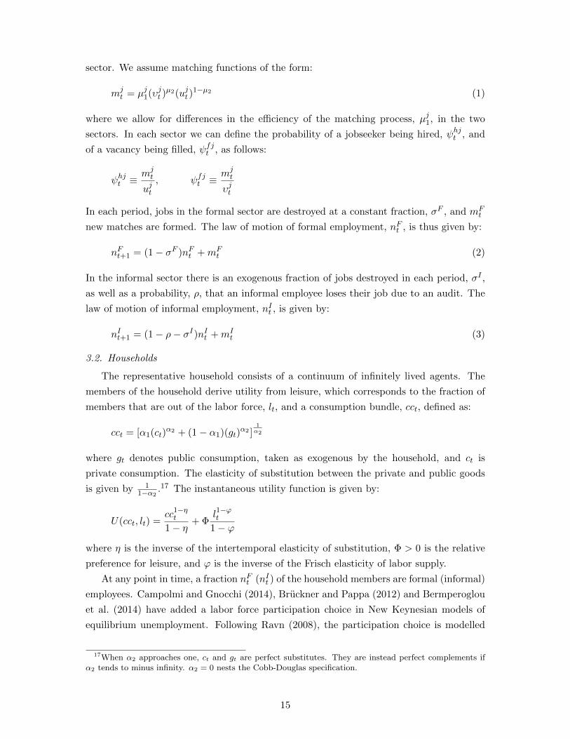
sector. We assume matching functions of the form:

mjt = µj1(υjt )

µ2(ujt )1−µ2 (1)

where we allow for differences in the efficiency of the matching process, µj1, in the two

sectors. In each sector we can define the probability of a jobseeker being hired, ψhjt , and

of a vacancy being filled, ψfjt , as follows:

ψhjt ≡mjt

ujt, ψfjt ≡

mjt

υjt

In each period, jobs in the formal sector are destroyed at a constant fraction, σF , and mFt

new matches are formed. The law of motion of formal employment, nFt , is thus given by:

nFt+1 = (1− σF )nFt +mFt (2)

In the informal sector there is an exogenous fraction of jobs destroyed in each period, σI ,

as well as a probability, ρ, that an informal employee loses their job due to an audit. The

law of motion of informal employment, nIt , is given by:

nIt+1 = (1− ρ− σI)nIt +mIt (3)

3.2. Households

The representative household consists of a continuum of infinitely lived agents. The

members of the household derive utility from leisure, which corresponds to the fraction of

members that are out of the labor force, lt, and a consumption bundle, cct, defined as:

cct = [α1(ct)α2 + (1− α1)(gt)

α2 ]1α2

where gt denotes public consumption, taken as exogenous by the household, and ct is

private consumption. The elasticity of substitution between the private and public goods

is given by 11−α2

.17 The instantaneous utility function is given by:

U(cct, lt) =cc1−ηt

1− η+ Φ

l1−ϕt

1− ϕ

where η is the inverse of the intertemporal elasticity of substitution, Φ > 0 is the relative

preference for leisure, and ϕ is the inverse of the Frisch elasticity of labor supply.

At any point in time, a fraction nFt (nIt ) of the household members are formal (informal)

employees. Campolmi and Gnocchi (2014), Bruckner and Pappa (2012) and Bermperoglou

et al. (2014) have added a labor force participation choice in New Keynesian models of

equilibrium unemployment. Following Ravn (2008), the participation choice is modelled

17When α2 approaches one, ct and gt are perfect substitutes. They are instead perfect complements ifα2 tends to minus infinity. α2 = 0 nests the Cobb-Douglas specification.

15

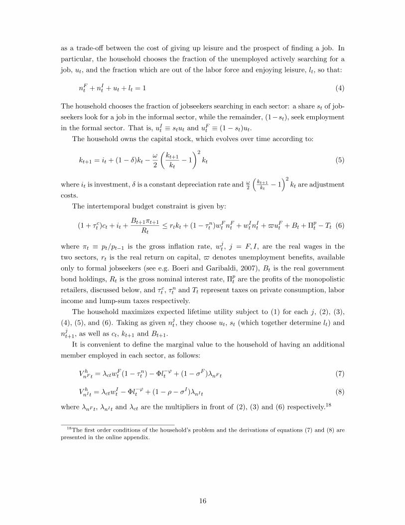
as a trade-off between the cost of giving up leisure and the prospect of finding a job. In

particular, the household chooses the fraction of the unemployed actively searching for a

job, ut, and the fraction which are out of the labor force and enjoying leisure, lt, so that:

nFt + nIt + ut + lt = 1 (4)

The household chooses the fraction of jobseekers searching in each sector: a share st of job-

seekers look for a job in the informal sector, while the remainder, (1−st), seek employment

in the formal sector. That is, uIt ≡ stut and uFt ≡ (1− st)ut.The household owns the capital stock, which evolves over time according to:

kt+1 = it + (1− δ)kt −ω

2

(kt+1

kt− 1

)2

kt (5)

where it is investment, δ is a constant depreciation rate and ω2

(kt+1

kt− 1)2kt are adjustment

costs.

The intertemporal budget constraint is given by:

(1 + τ ct )ct + it +Bt+1πt+1

Rt≤ rtkt + (1− τnt )wFt n

Ft +wIt n

It +$uFt +Bt + Πp

t − Tt (6)

where πt ≡ pt/pt−1 is the gross inflation rate, wjt , j = F, I, are the real wages in the

two sectors, rt is the real return on capital, $ denotes unemployment benefits, available

only to formal jobseekers (see e.g. Boeri and Garibaldi, 2007), Bt is the real government

bond holdings, Rt is the gross nominal interest rate, Πpt are the profits of the monopolistic

retailers, discussed below, and τ ct , τnt and Tt represent taxes on private consumption, labor

income and lump-sum taxes respectively.

The household maximizes expected lifetime utility subject to (1) for each j, (2), (3),

(4), (5), and (6). Taking as given njt , they choose ut, st (which together determine lt) and

njt+1, as well as ct, kt+1 and Bt+1.

It is convenient to define the marginal value to the household of having an additional

member employed in each sector, as follows:

V hnF t = λctw

Ft (1− τnt )− Φl−ϕt + (1− σF )λnF t (7)

V hnI t = λctw

It − Φl−ϕt + (1− ρ− σI)λnI t (8)

where λnF t, λnI t and λct are the multipliers in front of (2), (3) and (6) respectively.18

18The first order conditions of the household’s problem and the derivations of equations (7) and (8) arepresented in the online appendix.

16

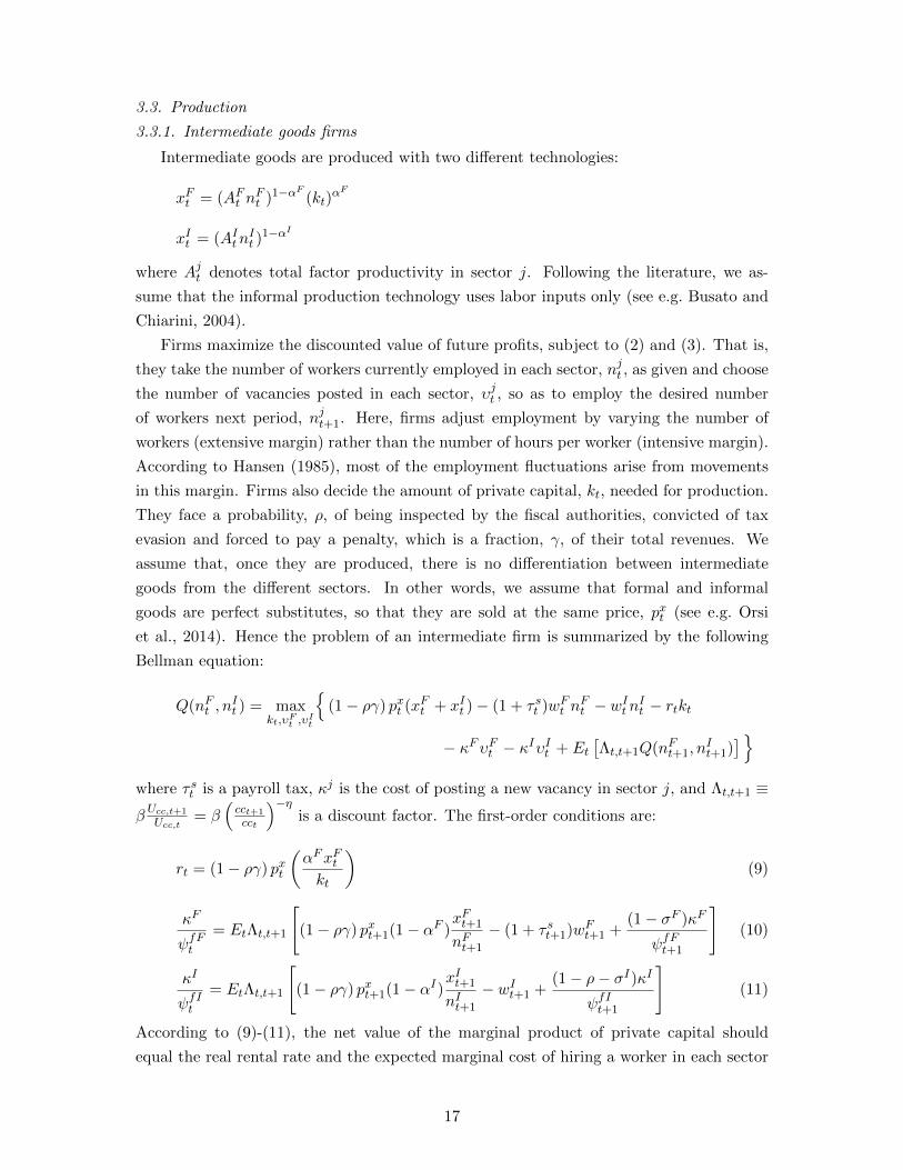
3.3. Production

3.3.1. Intermediate goods firms

Intermediate goods are produced with two different technologies:

xFt = (AFt nFt )1−αF (kt)

αF

xIt = (AItnIt )

1−αI

where Ajt denotes total factor productivity in sector j. Following the literature, we as-

sume that the informal production technology uses labor inputs only (see e.g. Busato and

Chiarini, 2004).

Firms maximize the discounted value of future profits, subject to (2) and (3). That is,

they take the number of workers currently employed in each sector, njt , as given and choose

the number of vacancies posted in each sector, υjt , so as to employ the desired number

of workers next period, njt+1. Here, firms adjust employment by varying the number of

workers (extensive margin) rather than the number of hours per worker (intensive margin).

According to Hansen (1985), most of the employment fluctuations arise from movements

in this margin. Firms also decide the amount of private capital, kt, needed for production.

They face a probability, ρ, of being inspected by the fiscal authorities, convicted of tax

evasion and forced to pay a penalty, which is a fraction, γ, of their total revenues. We

assume that, once they are produced, there is no differentiation between intermediate

goods from the different sectors. In other words, we assume that formal and informal

goods are perfect substitutes, so that they are sold at the same price, pxt (see e.g. Orsi

et al., 2014). Hence the problem of an intermediate firm is summarized by the following

Bellman equation:

Q(nFt , nIt ) = max

kt,υFt ,υIt

{(1− ργ) pxt (xFt + xIt )− (1 + τ st )wFt n

Ft − wIt nIt − rtkt

− κFυFt − κIυIt + Et[Λt,t+1Q(nFt+1, n

It+1)

] }where τ st is a payroll tax, κj is the cost of posting a new vacancy in sector j, and Λt,t+1 ≡βUcc,t+1

Ucc,t= β

(cct+1

cct

)−ηis a discount factor. The first-order conditions are:

rt = (1− ργ) pxt

(αFxFtkt

)(9)

κF

ψfFt= EtΛt,t+1

[(1− ργ) pxt+1(1− αF )

xFt+1

nFt+1

− (1 + τ st+1)wFt+1 +(1− σF )κF

ψfFt+1

](10)

κI

ψfIt= EtΛt,t+1

[(1− ργ) pxt+1(1− αI)

xIt+1

nIt+1

− wIt+1 +(1− ρ− σI)κI

ψfIt+1

](11)

According to (9)-(11), the net value of the marginal product of private capital should

equal the real rental rate and the expected marginal cost of hiring a worker in each sector

17

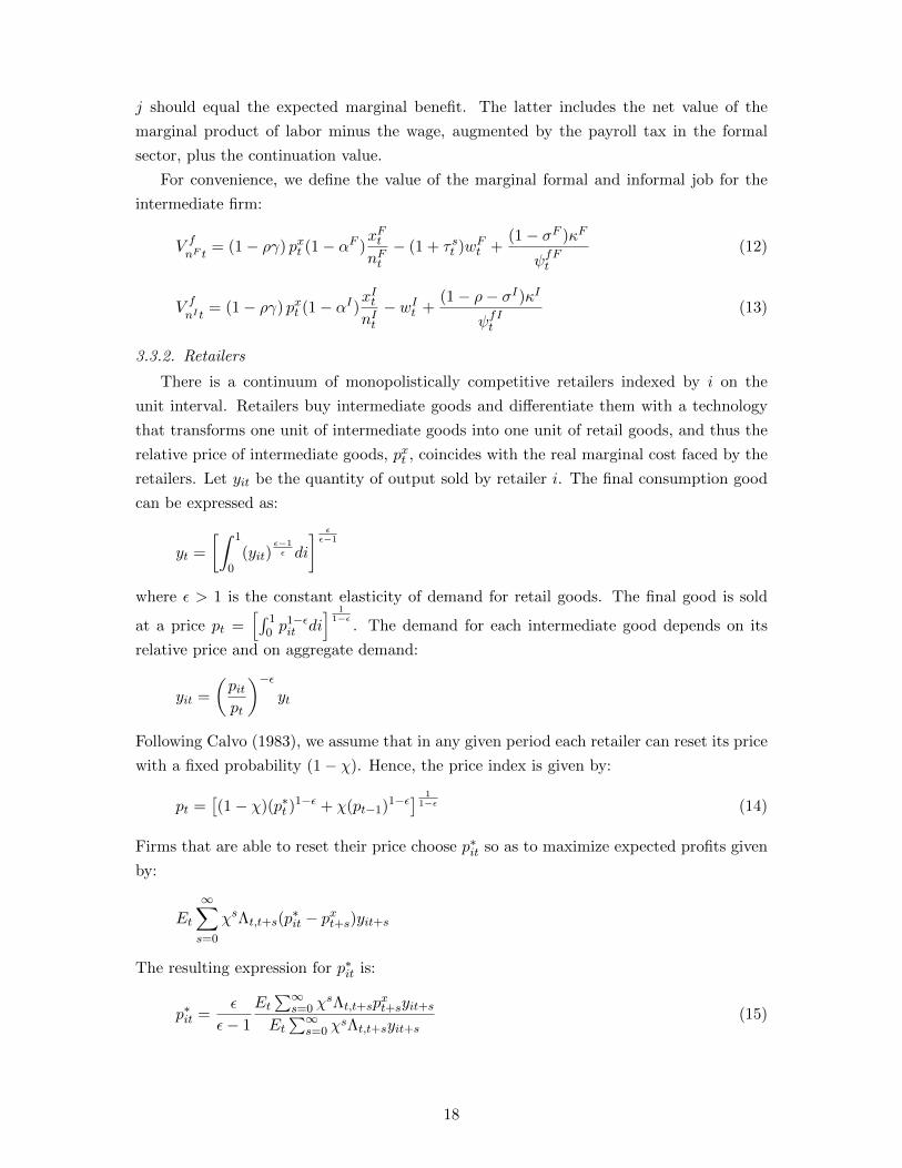
j should equal the expected marginal benefit. The latter includes the net value of the

marginal product of labor minus the wage, augmented by the payroll tax in the formal

sector, plus the continuation value.

For convenience, we define the value of the marginal formal and informal job for the

intermediate firm:

V fnF t

= (1− ργ) pxt (1− αF )xFtnFt− (1 + τ st )wFt +

(1− σF )κF

ψfFt(12)

V fnI t

= (1− ργ) pxt (1− αI)xIt

nIt− wIt +

(1− ρ− σI)κI

ψfIt(13)

3.3.2. Retailers

There is a continuum of monopolistically competitive retailers indexed by i on the

unit interval. Retailers buy intermediate goods and differentiate them with a technology

that transforms one unit of intermediate goods into one unit of retail goods, and thus the

relative price of intermediate goods, pxt , coincides with the real marginal cost faced by the

retailers. Let yit be the quantity of output sold by retailer i. The final consumption good

can be expressed as:

yt =

[∫ 1

0(yit)

ε−1ε di

] εε−1

where ε > 1 is the constant elasticity of demand for retail goods. The final good is sold

at a price pt =[∫ 1

0 p1−εit di

] 11−ε

. The demand for each intermediate good depends on its

relative price and on aggregate demand:

yit =

(pitpt

)−εyt

Following Calvo (1983), we assume that in any given period each retailer can reset its price

with a fixed probability (1− χ). Hence, the price index is given by:

pt =[(1− χ)(p∗t )

1−ε + χ(pt−1)1−ε] 11−ε (14)

Firms that are able to reset their price choose p∗it so as to maximize expected profits given

by:

Et

∞∑s=0

χsΛt,t+s(p∗it − pxt+s)yit+s

The resulting expression for p∗it is:

p∗it =ε

ε− 1

Et∑∞

s=0 χsΛt,t+sp

xt+syit+s

Et∑∞

s=0 χsΛt,t+syit+s

(15)

18

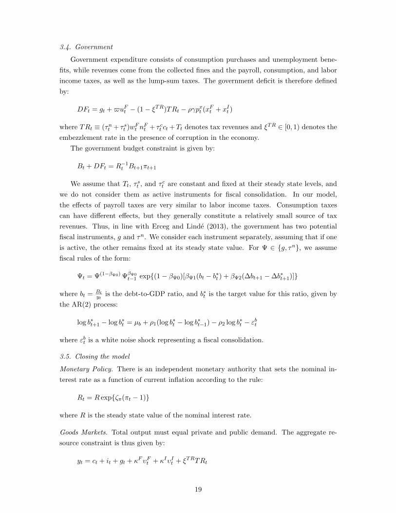
3.4. Government

Government expenditure consists of consumption purchases and unemployment bene-

fits, while revenues come from the collected fines and the payroll, consumption, and labor

income taxes, as well as the lump-sum taxes. The government deficit is therefore defined

by:

DFt = gt +$uFt − (1− ξTR)TRt − ργpxt (xFt + xIt )

where TRt ≡ (τnt + τ st )wFt nFt + τ ct ct +Tt denotes tax revenues and ξTR ∈ [0, 1) denotes the

embezzlement rate in the presence of corruption in the economy.

The government budget constraint is given by:

Bt +DFt = R−1t Bt+1πt+1

We assume that Tt, τst , and τ ct are constant and fixed at their steady state levels, and

we do not consider them as active instruments for fiscal consolidation. In our model,

the effects of payroll taxes are very similar to labor income taxes. Consumption taxes

can have different effects, but they generally constitute a relatively small source of tax

revenues. Thus, in line with Erceg and Linde (2013), the government has two potential

fiscal instruments, g and τn. We consider each instrument separately, assuming that if one

is active, the other remains fixed at its steady state value. For Ψ ∈ {g, τn}, we assume

fiscal rules of the form:

Ψt = Ψ(1−βΨ0) ΨβΨ0t−1 exp{(1− βΨ0)[βΨ1(bt − b∗t ) + βΨ2(∆bt+1 −∆b∗t+1)]}

where bt = Btyt

is the debt-to-GDP ratio, and b∗t is the target value for this ratio, given by

the AR(2) process:

log b∗t+1 − log b∗t = µb + ρ1(log b∗t − log b∗t−1)− ρ2 log b∗t − εbt

where εbt is a white noise shock representing a fiscal consolidation.

3.5. Closing the model

Monetary Policy. There is an independent monetary authority that sets the nominal in-

terest rate as a function of current inflation according to the rule:

Rt = R exp{ζπ(πt − 1)}

where R is the steady state value of the nominal interest rate.

Goods Markets. Total output must equal private and public demand. The aggregate re-

source constraint is thus given by:

yt = ct + it + gt + κFυFt + κIυIt + ξTRTRt

19

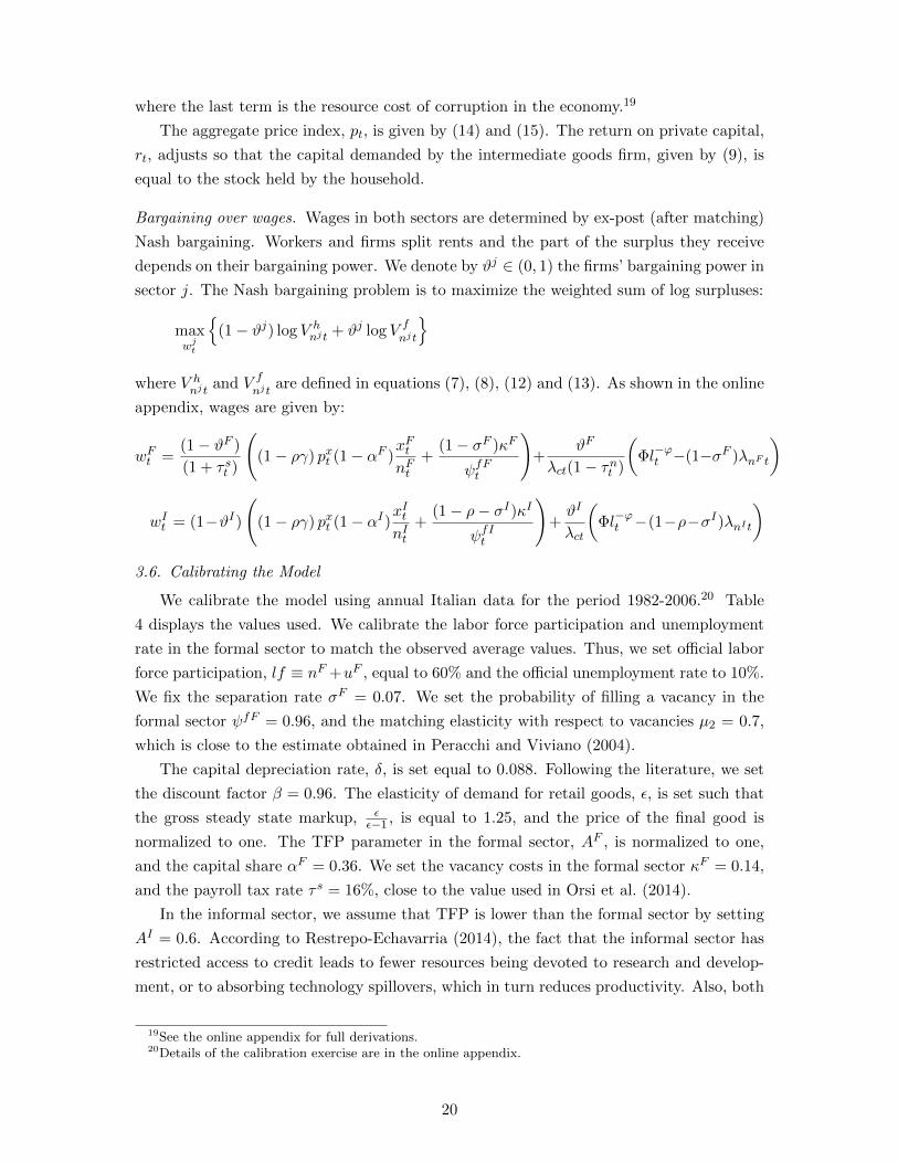
where the last term is the resource cost of corruption in the economy.19

The aggregate price index, pt, is given by (14) and (15). The return on private capital,

rt, adjusts so that the capital demanded by the intermediate goods firm, given by (9), is

equal to the stock held by the household.

Bargaining over wages. Wages in both sectors are determined by ex-post (after matching)

Nash bargaining. Workers and firms split rents and the part of the surplus they receive

depends on their bargaining power. We denote by ϑj ∈ (0, 1) the firms’ bargaining power in

sector j. The Nash bargaining problem is to maximize the weighted sum of log surpluses:

maxwjt

{(1− ϑj) log V h

njt + ϑj log V fnjt

}where V h

njtand V f

njtare defined in equations (7), (8), (12) and (13). As shown in the online

appendix, wages are given by:

wFt =(1− ϑF )

(1 + τ st )

((1− ργ) pxt (1− αF )

xFtnFt

+(1− σF )κF

ψfFt

)+

ϑF

λct(1− τnt )

(Φl−ϕt −(1−σF )λnF t

)

wIt = (1−ϑI)

((1− ργ) pxt (1− αI)x

It

nIt+

(1− ρ− σI)κI

ψfIt

)+ϑI

λct

(Φl−ϕt −(1−ρ−σI)λnI t

)3.6. Calibrating the Model

We calibrate the model using annual Italian data for the period 1982-2006.20 Table

4 displays the values used. We calibrate the labor force participation and unemployment

rate in the formal sector to match the observed average values. Thus, we set official labor

force participation, lf ≡ nF +uF , equal to 60% and the official unemployment rate to 10%.

We fix the separation rate σF = 0.07. We set the probability of filling a vacancy in the

formal sector ψfF = 0.96, and the matching elasticity with respect to vacancies µ2 = 0.7,

which is close to the estimate obtained in Peracchi and Viviano (2004).

The capital depreciation rate, δ, is set equal to 0.088. Following the literature, we set

the discount factor β = 0.96. The elasticity of demand for retail goods, ε, is set such that

the gross steady state markup, εε−1 , is equal to 1.25, and the price of the final good is

normalized to one. The TFP parameter in the formal sector, AF , is normalized to one,

and the capital share αF = 0.36. We set the vacancy costs in the formal sector κF = 0.14,

and the payroll tax rate τ s = 16%, close to the value used in Orsi et al. (2014).

In the informal sector, we assume that TFP is lower than the formal sector by setting

AI = 0.6. According to Restrepo-Echavarria (2014), the fact that the informal sector has

restricted access to credit leads to fewer resources being devoted to research and develop-

ment, or to absorbing technology spillovers, which in turn reduces productivity. Also, both

19See the online appendix for full derivations.20Details of the calibration exercise are in the online appendix.

20

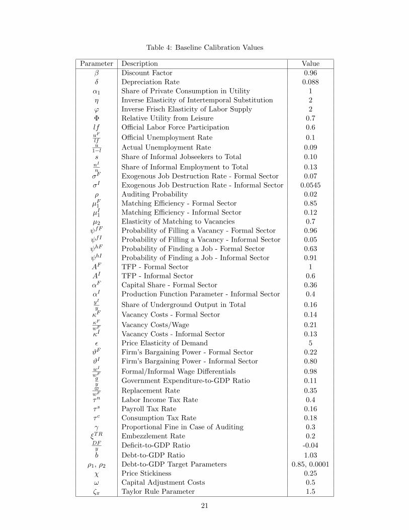
Table 4: Baseline Calibration Values

Parameter Description Value

β Discount Factor 0.96δ Depreciation Rate 0.088α1 Share of Private Consumption in Utility 1η Inverse Elasticity of Intertemporal Substitution 2ϕ Inverse Frisch Elasticity of Labor Supply 2Φ Relative Utility from Leisure 0.7lf Official Labor Force Participation 0.6uF

lf Official Unemployment Rate 0.1u

1−l Actual Unemployment Rate 0.09

s Share of Informal Jobseekers to Total 0.10nI

n Share of Informal Employment to Total 0.13σF Exogenous Job Destruction Rate - Formal Sector 0.07σI Exogenous Job Destruction Rate - Informal Sector 0.0545ρ Auditing Probability 0.02µF1 Matching Efficiency - Formal Sector 0.85µI1 Matching Efficiency - Informal Sector 0.12µ2 Elasticity of Matching to Vacancies 0.7ψfF Probability of Filling a Vacancy - Formal Sector 0.96ψfI Probability of Filling a Vacancy - Informal Sector 0.05ψhF Probability of Finding a Job - Formal Sector 0.63ψhI Probability of Finding a Job - Informal Sector 0.91AF TFP - Formal Sector 1AI TFP - Informal Sector 0.6αF Capital Share - Formal Sector 0.36αI Production Function Parameter - Informal Sector 0.4yI

y Share of Underground Output in Total 0.16

κF Vacancy Costs - Formal Sector 0.14κF

wFVacancy Costs/Wage 0.21

κI Vacancy Costs - Informal Sector 0.13ε Price Elasticity of Demand 5ϑF Firm’s Bargaining Power - Formal Sector 0.22ϑI Firm’s Bargaining Power - Informal Sector 0.80wI

wFFormal/Informal Wage Differentials 0.98

gy Government Expenditure-to-GDP Ratio 0.11$wF

Replacement Rate 0.35

τn Labor Income Tax Rate 0.4τ s Payroll Tax Rate 0.16τ c Consumption Tax Rate 0.18γ Proportional Fine in Case of Auditing 0.3ξTR Embezzlement Rate 0.2DFy Deficit-to-GDP Ratio -0.04

b Debt-to-GDP Ratio 1.03ρ1, ρ2 Debt-to-GDP Target Parameters 0.85, 0.0001χ Price Stickiness 0.25ω Capital Adjustment Costs 0.5ζπ Taylor Rule Parameter 1.5

21

Boeri and Garibaldi (2007) and Orsi et al. (2014) emphasize empirical evidence suggesting

that the workers in the informal sector have lower education levels.21

Using the ISTAT data, we set the share of informal employment to total employment

equal to 0.13, and we set αI = 0.4, implying the share of shadow output to total outputyI

y = 16%. We set the exogenous job destruction rate in the informal sector σI = 0.0545,

the probability of filling a vacancy in the informal sector ψfI = 0.05, and the vacancy cost

in the informal sector κI = 0.13. These values yield a relatively small wage premium for

the formal sector, wI

wF= 0.98, in line with the literature. The probability of audit and the

fraction of total revenues paid as a fine in the event of an audit are set as follows: ρ = 0.02,

close to the value used in Boeri and Garibaldi (2007), and γ = 0.3. For the probability

of tax audit, we also consider alternative values (ρ = 0.04 and ρ = 0.01) in the sensitivity

analysis.

We set the replacement rate $wF

= 0.35, close to the estimates in Martin (1996), and

used by Fugazza and Jacques (2004). Government spending as a share of GDP and the

remaining tax rates are set as follows: gy = 11%, τn = 40%, in line with Orsi et al.

(2014), and τ c = 18%. The steady state debt-to-GDP ratio b = 103%. Regarding the

embezzlement parameter, we set ξTR = 0.2 and study the sensitivity of our results to

different values of this parameter.

We begin by assuming purely wasteful government expenditure, setting α1 = 1, and

will consider utility enhancing government spending as an extension. Regarding the inverse

elasticity of intertemporal substitution, η, much of the literature cites the econometric

estimates of Hansen and Singleton (1983), which place it “between 0 and 2”, and often

choose a value greater than unity. In our calibration, we set η = 2 and we perform

sensitivity analysis by considering η equal to 0.5 and 1. The inverse of the Frisch elasticity,

ϕ, is set equal to 2 and we examine the sensitivity of our results to changes in this parameter.

Finally, we set the inflation targeting parameter in the Taylor rule ζπ = 1.5, the capital

adjustment costs ω = 0.5 and the price-stickiness parameter χ = 0.25.

4. Results

We present responses following a negative debt-target shock (following Erceg and Linde,

2013). We compare the effects of a 5% reduction in the desired long run debt target, which

is achieved after 10 years, either through a fall in government consumption expenditure,

or a hike in labor tax rates.22

4.1. Dynamics in a Model without Tax Evasion and Corruption

As a benchmark, we begin by analyzing the responses of a standard model where tax

evasion and corruption are absent, shown in Figure 5.

21Orsi et al. (2014) also note the equivalence of assuming lower productivity in the informal sector toassuming a cost for concealing production.

22For comparison purposes, throughout this section we adjust the parameters of the policy rules for eachcase to ensure that the debt target is met after 10 years.

22

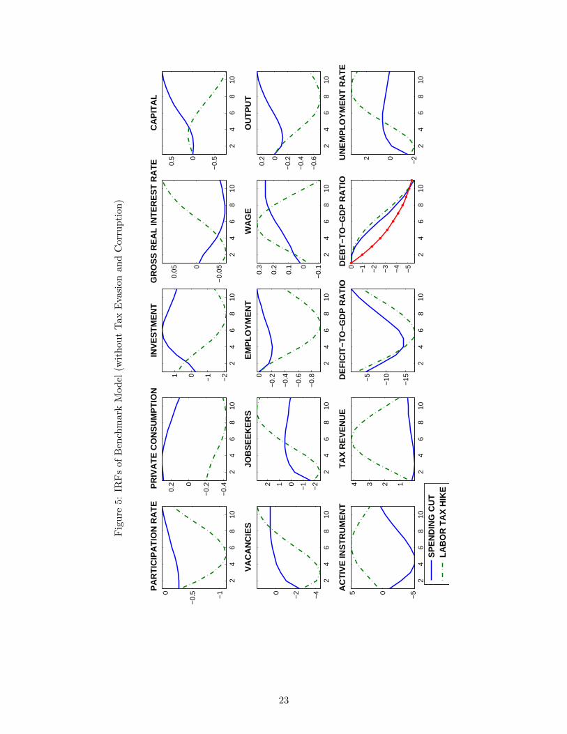
Fig

ure

5:IR

Fs

ofB

ench

mar

kM

od

el(w

ith

out

Tax

Eva

sion

and

Cor

rup

tion

)

24

68

10

−1

−0.

50PA

RT

ICIP

AT

ION

RA

TE

24

68

10−

0.4

−0.

20

0.2PR

IVA

TE

CO

NS

UM

PT

ION

24

68

10−

2

−101

INV

ES

TM

EN

T

24

68

10

−0.

050

0.05

GR

OS

S R

EA

L IN

TE

RE

ST

RA

TE

24

68

10

−0.

50

0.5

CA

PIT

AL

24

68

10

−4

−20

VA

CA

NC

IES

24

68

10

−2

−1012

JOB

SE

EK

ER

S

24

68

10

−0.

8

−0.

6

−0.

4

−0.

20

EM

PLO

YM

EN

T

24

68

10−

0.10

0.1

0.2

0.3

WA

GE

24

68

10

−0.

6

−0.

4

−0.

20

0.2

OU

TP

UT

24

68

10−

505AC

TIV

E IN

ST

RU

ME

NT

24

68

10

1234

TA

X R

EV

EN

UE

24

68

10

−15

−10−

5DE

FIC

IT−T

O−G

DP

RA

TIO

24

68

10

−5

−4

−3

−2

−10D

EB

T−T

O−G

DP

RA

TIO

24

68

10−

202UN

EM

PLO

YM

EN

T R

AT

E

SP

EN

DIN

G C

UT

LAB

OR

TA

X H

IKE

23

A consolidation carried out through a fall in government spending has two effects.

Firstly, there is a negative demand effect for firms, which leads, in the presence of nominal

rigidities, to a fall in labor demand and hence in vacancies. Second, there is a positive

wealth effect for the household, which increases consumption and investment and reduces

labor force participation. Given the drop in both labor demand and supply, employment

falls and the wage rate rises. Output falls in the short run, but increases in the medium and

long run because investment, and hence the capital stock, increases. The unemployment

rate reflects movements in the number of jobseekers: it falls on impact, but then increases

as employment and wages adjust.

When the fiscal consolidation is carried out through a labor tax hike, there is a negative

wealth effect for the household which makes consumption fall, and investment fall with a

lag. However, as the return from employment falls, there is a substitution effect which

outweighs the wealth effect, and leads to a decrease in labor force participation. The fall in

private demand induces firms to contract their labor demand, again expressed through a

drop in vacancies. Employment and output fall, and the responses are significantly larger

and more persistent than in the case of spending cuts, due to the fall in investment.

Thus, our benchmark model seems to be consistent with the evidence of Alesina et al.

(2013): spending cuts are accompanied by mild and short-lived recessions, while tax hikes

lead to more prolonged and deep recessions.

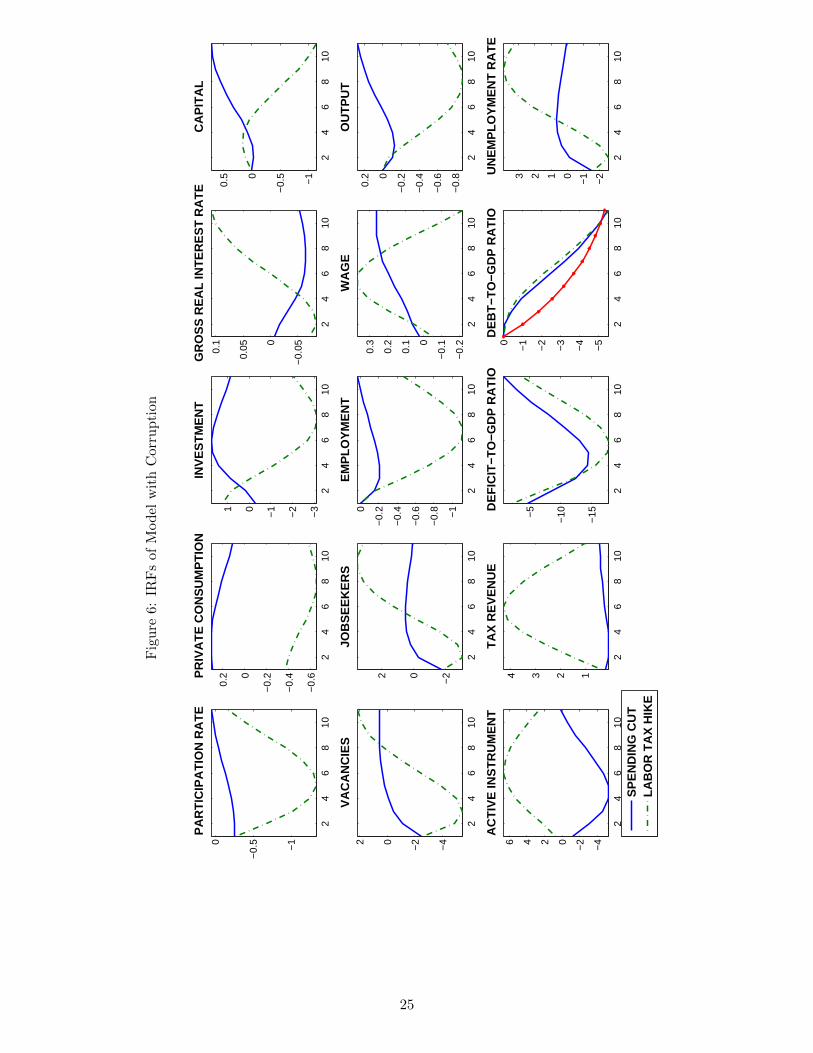
4.2. Dynamics in a Model with Corruption

Next, we study how the responses change when we introduce embezzlement of public

funds in our model, shown in Figure 6. In our baseline calibration we set the embezzlement

rate ξTR = 0.2.

The introduction of corruption does not alter the responses of the economy qualitatively.

In the case of government spending cuts, the effects are negligible. However, in the case

of labor tax rate hikes, there are notable quantitative differences. Given that a fraction of

tax revenues are now lost through embezzlement, the change in the tax rates required to

achieve debt consolidation is larger. This leads to an amplification of the effects observed

in all variables.

We also check the sensitivity of this effect to the embezzlement rate. Informal accounts

suggest that there are often large rents to be obtained in less developed economies, although

precise estimates are difficult to obtain. Krueger (1974) estimates rents generated by

import licenses alone to be in the range of 15% of GNP for Turkey in 1968; similarly

large estimates are obtained by Gallagher (1991) for a sample of African countries from

1975 to 1987, ranging between 6% and 37% of GDP. Setting ξTR = 0.2 implies a value of

embezzled tax revenues equal to 4.2% of GDP. Given the estimates for developing countries,

we believe that a reasonable range of estimates of rent seeking as a percentage of GDP in

Italy should be between 0.1% and 5%. This implies values for ξTR that vary between 0.05

and 0.25. Results for this sensitivity analysis, presented in the online appendix, show that

24

Fig

ure

6:IR

Fs

ofM

od

elw

ith

Cor

rup

tion

24

68

10

−1

−0.

50

PA

RT

ICIP

AT

ION

RA

TE

24

68

10−

0.6

−0.

4

−0.

20

0.2P

RIV

AT

E C

ON

SU

MP

TIO

N

24

68

10−

3

−2

−101

INV

ES

TM

EN

T

24

68

10

−0.

050

0.050.

1

GR

OS

S R

EA

L IN

TE

RE

ST

RA

TE

24

68

10

−1

−0.

50

0.5

CA

PIT

AL

24

68

10

−4

−202

VA

CA

NC

IES

24

68

10

−202

JOB

SE

EK

ER

S

24

68

10

−1

−0.

8

−0.

6

−0.

4

−0.

20

EM

PLO

YM

EN

T

24

68

10−

0.2

−0.

10

0.1

0.2

0.3

WA

GE

24

68

10

−0.

8

−0.

6

−0.

4

−0.

20

0.2

OU

TP

UT

24

68

10

−4

−20246

AC

TIV

E IN

ST

RU

ME

NT

24

68

10

1234

TA

X R

EV

EN

UE

24

68

10

−15

−10−

5DE

FIC

IT−T

O−G

DP

RA

TIO

24

68

10

−5

−4

−3

−2

−10

DE

BT

−TO

−GD

P R

AT

IO

24

68

10

−2

−10123U

NE

MP

LOY

ME

NT

RA

TE

SP

EN

DIN

G C

UT

LAB

OR

TA

X H

IKE

25

with the higher the degree of corruption in the economy, the larger the tax hikes needed

for consolidation and therefore the larger the amplification of the observed responses.

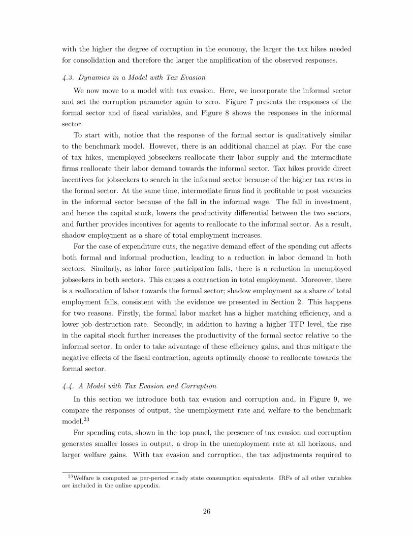
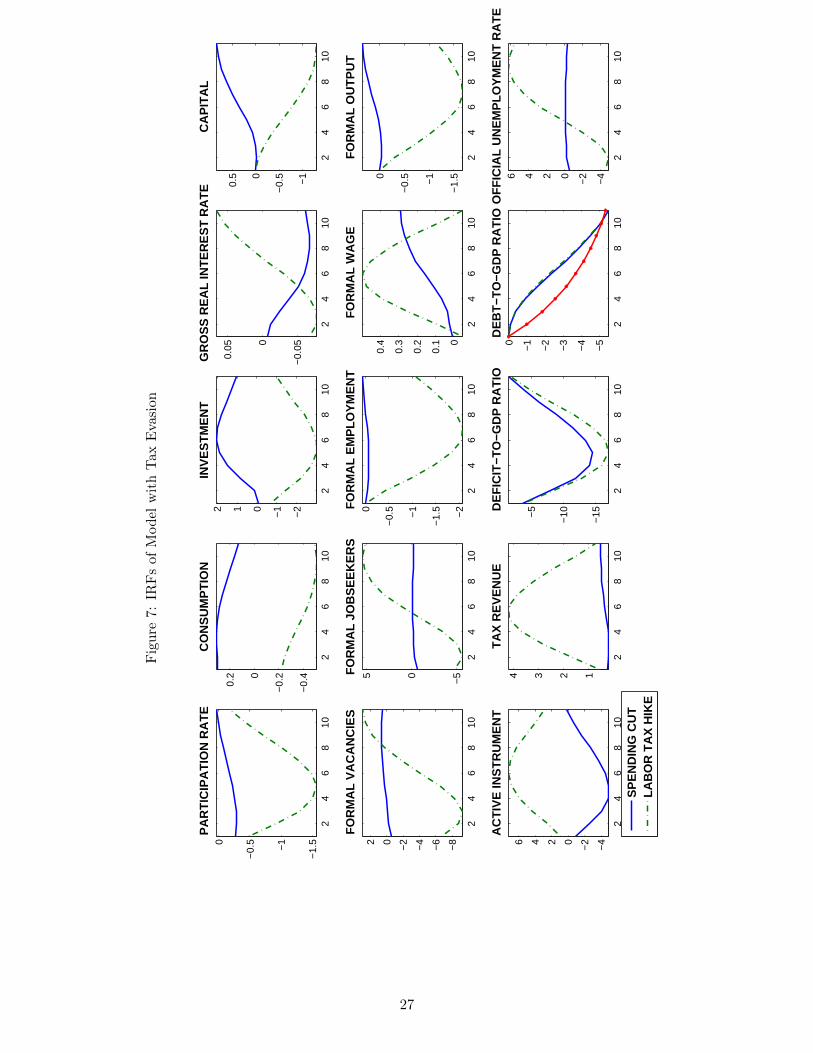
4.3. Dynamics in a Model with Tax Evasion

We now move to a model with tax evasion. Here, we incorporate the informal sector

and set the corruption parameter again to zero. Figure 7 presents the responses of the

formal sector and of fiscal variables, and Figure 8 shows the responses in the informal

sector.

To start with, notice that the response of the formal sector is qualitatively similar

to the benchmark model. However, there is an additional channel at play. For the case

of tax hikes, unemployed jobseekers reallocate their labor supply and the intermediate

firms reallocate their labor demand towards the informal sector. Tax hikes provide direct

incentives for jobseekers to search in the informal sector because of the higher tax rates in

the formal sector. At the same time, intermediate firms find it profitable to post vacancies

in the informal sector because of the fall in the informal wage. The fall in investment,

and hence the capital stock, lowers the productivity differential between the two sectors,

and further provides incentives for agents to reallocate to the informal sector. As a result,

shadow employment as a share of total employment increases.

For the case of expenditure cuts, the negative demand effect of the spending cut affects

both formal and informal production, leading to a reduction in labor demand in both

sectors. Similarly, as labor force participation falls, there is a reduction in unemployed

jobseekers in both sectors. This causes a contraction in total employment. Moreover, there

is a reallocation of labor towards the formal sector; shadow employment as a share of total

employment falls, consistent with the evidence we presented in Section 2. This happens

for two reasons. Firstly, the formal labor market has a higher matching efficiency, and a

lower job destruction rate. Secondly, in addition to having a higher TFP level, the rise

in the capital stock further increases the productivity of the formal sector relative to the

informal sector. In order to take advantage of these efficiency gains, and thus mitigate the

negative effects of the fiscal contraction, agents optimally choose to reallocate towards the

formal sector.

4.4. A Model with Tax Evasion and Corruption

In this section we introduce both tax evasion and corruption and, in Figure 9, we

compare the responses of output, the unemployment rate and welfare to the benchmark

model.23

For spending cuts, shown in the top panel, the presence of tax evasion and corruption

generates smaller losses in output, a drop in the unemployment rate at all horizons, and

larger welfare gains. With tax evasion and corruption, the tax adjustments required to

23Welfare is computed as per-period steady state consumption equivalents. IRFs of all other variablesare included in the online appendix.

26

Fig

ure

7:IR

Fs

ofM

od

elw

ith

Tax

Eva

sion

24

68

10−

1.5

−1

−0.

50

PA

RT

ICIP

AT

ION

RA

TE

24

68

10

−0.

4

−0.

20

0.2

CO

NS

UM

PT

ION

24

68

10

−2

−1012

INV

ES

TM

EN

T

24

68

10

−0.

050

0.05

GR

OS

S R

EA

L IN

TE

RE

ST

RA

TE

24

68

10

−1

−0.

50

0.5

CA

PIT

AL

24

68

10

−8

−6

−4

−202

FO

RM

AL

VA

CA

NC

IES

24

68

10

−505F

OR

MA

L JO

BS

EE

KE

RS

24

68

10−

2

−1.

5

−1

−0.

50FO

RM

AL

EM

PLO

YM

EN

T

24

68

10

0

0.1

0.2

0.3

0.4

FO

RM

AL

WA

GE

24

68

10

−1.

5

−1

−0.

50

FO

RM

AL

OU

TP

UT

24

68

10

−4

−20246

AC

TIV

E IN

ST

RU

ME

NT

24

68

10

1234

TA

X R

EV

EN

UE

24

68

10

−15

−10−

5DE

FIC

IT−T

O−G

DP

RA

TIO

24

68

10

−5

−4

−3

−2

−10

DE

BT

−TO

−GD

P R

AT

IO

24

68

10

−4

−20246

OF

FIC

IAL

UN

EM

PLO

YM

EN

T R

AT

E

SP

EN

DIN

G C

UT

LAB

OR

TA

X H

IKE

27

Fig

ure

8:IR

Fs

ofM

od

elw

ith

Tax

Eva

sion

-In

form

alS

ecto

r

24

68

10

−505101520

UN

DE

RG

RO

UN

D V

AC

AN

CIE

S

24

68

10

−50510152025

UN

DE

RG

RO

UN

D J

OB

SE

EK

ER

S

24

68

10

−2.

5

−2

−1.

5

−1

−0.

50

UN

DE

RG

RO

UN

D W

AG

E

24

68

10

0123456

UN

DE

RG

RO

UN

D E

MP

LO

YM

EN

T

24

68

10

0

0.51

1.52

2.53

3.5

UN

DE

RG

RO

UN

D O

UT

PU

T

SP

EN

DIN

G C

UT

LA

BO

R T

AX

HIK

E

28

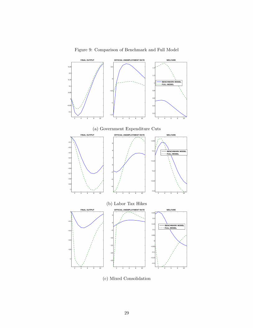
Figure 9: Comparison of Benchmark and Full Model

2 4 6 8 10

−0.1

−0.05

0

0.05

0.1

0.15

0.2

0.25

FINAL OUTPUT

2 4 6 8 10

−1.5

−1

−0.5

0

0.5

OFFICIAL UNEMPLOYMENT RATE

2 4 6 8 10

0.2

0.4

0.6

0.8

1

1.2

1.4

WELFARE

BENCHMARK MODELFULL MODEL

(a) Government Expenditure Cuts

2 4 6 8 10

−1

−0.9

−0.8

−0.7

−0.6

−0.5

−0.4

−0.3

−0.2

−0.1

0FINAL OUTPUT

2 4 6 8 10

−6

−4

−2

0

2

4

6

OFFICIAL UNEMPLOYMENT RATE

2 4 6 8 10

−0.3

−0.25

−0.2

−0.15

−0.1

−0.05

WELFARE

BENCHMARK MODELFULL MODEL

(b) Labor Tax Hikes

2 4 6 8 10

−1

−0.8

−0.6

−0.4

−0.2

0FINAL OUTPUT

2 4 6 8 10

−25

−20

−15

−10

−5

0

5

OFFICIAL UNEMPLOYMENT RATE

2 4 6 8 10

−0.2

−0.15

−0.1

−0.05

0

0.05

0.1

0.15

0.2

0.25

WELFARE

BENCHMARK MODELFULL MODEL

(c) Mixed Consolidation

29

achieve a given change in deficit are larger, and thus, following a spending cut, taxes in the

future are expected to fall by more. In other words, there is an amplification of the positive

wealth effect. Hence the rise in consumption and the fall in labor force participation are

larger relative to the model without tax evasion and corruption, making welfare gains

larger. The increased crowding-in of private consumption mitigates the negative demand

effect for the firms, thereby mitigating output losses. The larger reduction in labor force

participation implies a fall in the number of formal jobseekers, and hence in the official

unemployment rate, at all horizons.

For tax hikes, shown in the middle panel, the presence of corruption and tax evasion

amplifies the output losses, particularly in the long run. This is due to the loss of tax

revenue from both corruption and tax evasion, implying that larger increases in tax rates are

needed to reduce debt-to-GDP. This increases the distortionary effects of the consolidation,

leading to a larger drop in labor force participation, private consumption and investment.

In addition, the reallocation towards the informal sector increases the inefficiencies due

to the lower productivity in this sector. Thus, there is a larger contraction in the formal

sector, which is also evident in the response of the official unemployment rate: the initial

fall is amplified as jobseekers drop out of the formal sector, and the rise in the long run is

higher as firms post fewer vacancies in this sector. Furthermore, tax hikes lead to welfare

losses. Initially, these losses are lower with tax evasion and corruption, but in the medium

and long run, as consumption falls increasingly, we obtain higher losses.

The bottom panel depicts the responses in the case of a mixed consolidation. Here, we

allow both policy instruments, g and τn, to move simultaneously to reduce the deficit, which

follows the debt-targeting rule. We fix the policy mix such that a fraction a of the reductions

in deficit come from expenditure cuts and (1 − a) from revenue enhancements, and set

a = 0.5. In this case, the responses of consumption and investment are determined by the

competing positive and negative wealth effects from the two instruments, and the presence

of tax evasion and corruption plays an important role in determining this relative strength.

In the benchmark model, the positive wealth effect of the expenditure cut is dominant and

consumption rises for several periods. When there is tax evasion and corruption, this is no

longer true and consumption and investment fall in all periods. Hence, as in the case of

tax hikes, output and unemployment responses are amplified in the presence of tax evasion

and corruption. This is in line with the evidence presented in Section 2. Moreover, the

welfare gains obtained from mixed consolidation packages in the benchmark model turn

into welfare losses in the model with tax evasion and corruption.

4.5. Sensitivity Analysis

Both the effects of labor tax hikes and expenditure cuts depend crucially on some mod-

eling assumptions. In this section we present how the implications of fiscal consolidations

change when we modify key assumptions or parameters of the model.

30

Figure 10: Sensitivity Analysis for Spending Cuts in the Full Model

5 10 15

−0.05

0

0.05

0.1

0.15

0.2

0.25

0.3

FINAL OUTPUT

5 10 15

−0.5

−0.4

−0.3

−0.2

−0.1

0

OFFICIAL UNEMPLOYMENT RATE

5 10 15

0.2

0.4

0.6

0.8

1

1.2

1.4

WELFARE

η = 2

η = 0.95

η = 0.5

(a) Intertemporal Elasticity of Substitution

2 4 6 8 10

−0.05

0

0.05

0.1

0.15

0.2

0.25

FINAL OUTPUT

2 4 6 8 10

−0.55

−0.5

−0.45

−0.4

−0.35

−0.3

−0.25

−0.2

−0.15

−0.1

−0.05

OFFICIAL UNEMPLOYMENT RATE

2 4 6 8 10

−0.2

0

0.2

0.4

0.6

0.8

1

1.2

1.4

WELFARE

WASTEFUL SPENDINGUTILITY ENHANCING SPENDING

(b) Utility Enhancing Government Spending

2 4 6 8 10

−0.1

0

0.1

0.2

0.3

0.4

FINAL OUTPUT

2 4 6 8 10

−1.2

−1

−0.8

−0.6

−0.4

−0.2

OFFICIAL UNEMPLOYMENT RATE

2 4 6 8 10

0.5

1

1.5

WELFARE

ONLY OPTIMIZING CONSUMERSOPTIMIZING AND ROT CONSUMERS

(c) Rule of Thumb (ROT) Consumers

31

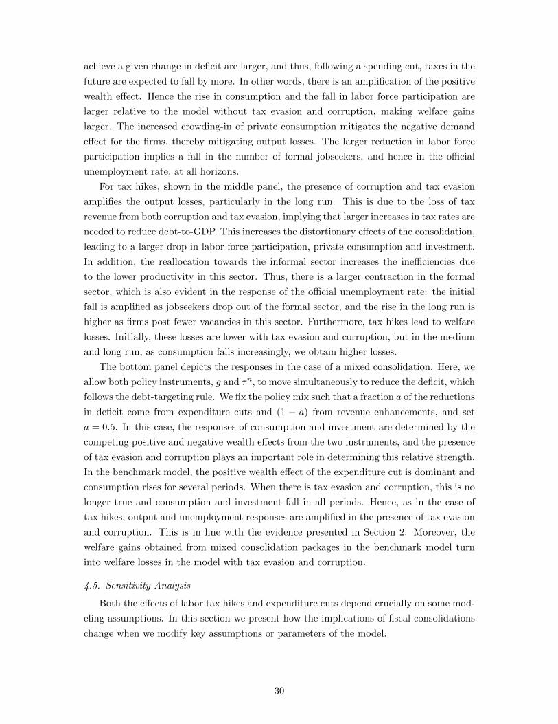
4.5.1. Spending Cuts

Elasticity of Intertemporal Substitution. As we saw, the effects of the spending cuts de-

pend crucially on the size of the wealth effect, which in turn depends on the elasticity of

intertemporal substitution. As shown in the first panel of Figure 10, repeating the simu-

lations using lower values for the inverse elasticity of intertemporal substitution, η = 0.5

and η = 0.95, yields qualitatively similar results. Quantitatively, for lower values of η,

the risk aversion of agents is lower and after a spending cut we observe larger increases in

consumption and smaller increases in investment, which dampens the long run expansion

in output, as well as a larger drop in the labor force participation rate, which dampens the

drop in the unemployment rate.

Utility-enhancing Government Spending. Assuming that government expenditures provide

a public good, which is consumed by households, can change the welfare implications of

spending cuts. To illustrate this point, we set α1 = 0.85 and α2 = −0.25, so that private

and public spending are weak complements. The top panel of Figure 10 compares the

results of this case with those obtained with wasteful government spending. In the case of

utility-enhancing expenditures, a spending cut directly reduces the consumption bundle,

and households are forced to offset this fall by further increasing private consumption.

Thus, we see a larger crowding-in of private consumption, which mitigates the output and

unemployment effects of spending cuts. However, the welfare effects are reversed: the drop

in the consumption bundle causes welfare to fall for several periods.

Liquidity Constrained Agents. The presence of liquidity constrained consumers has been

shown to play an important role in determining the response of private consumption to

a government spending cut (see e.g. Galı et al., 2007). To explore how the presence of

liquidity constrained consumers can affect our model, we assume a fraction of rule of thumb

(ROT) household members, which we set equal to 44%, in line with the Italian household

survey reported by Martin and Philippon (2014). As shown in the bottom panel of Figure

10, output and unemployment responses are amplified and welfare gains are mitigated

following a spending cut. The presence of ROT agents reduces the positive wealth effect

that the fiscal contraction generates, which implies a smaller increase in consumption and,

hence, welfare, and a larger contraction in output.

4.5.2. Tax Hikes

The Elasticity of Taxable Income. A large body of the literature, initiated by Feldstein

(1999), has argued that the costs of labor taxes can be summarized by the elasticity of

taxable income with respect to the net of tax share. The magnitude of this elasticity can

therefore yield further insights about the effects of tax hikes in the presence of tax evasion

and corruption. We compute the taxable income elasticity by dividing the cumulative

response of taxable income by the cumulative response of the net tax share, up to the point

that tax rates return to steady state. For the benchmark model, the elasticity of taxable

32

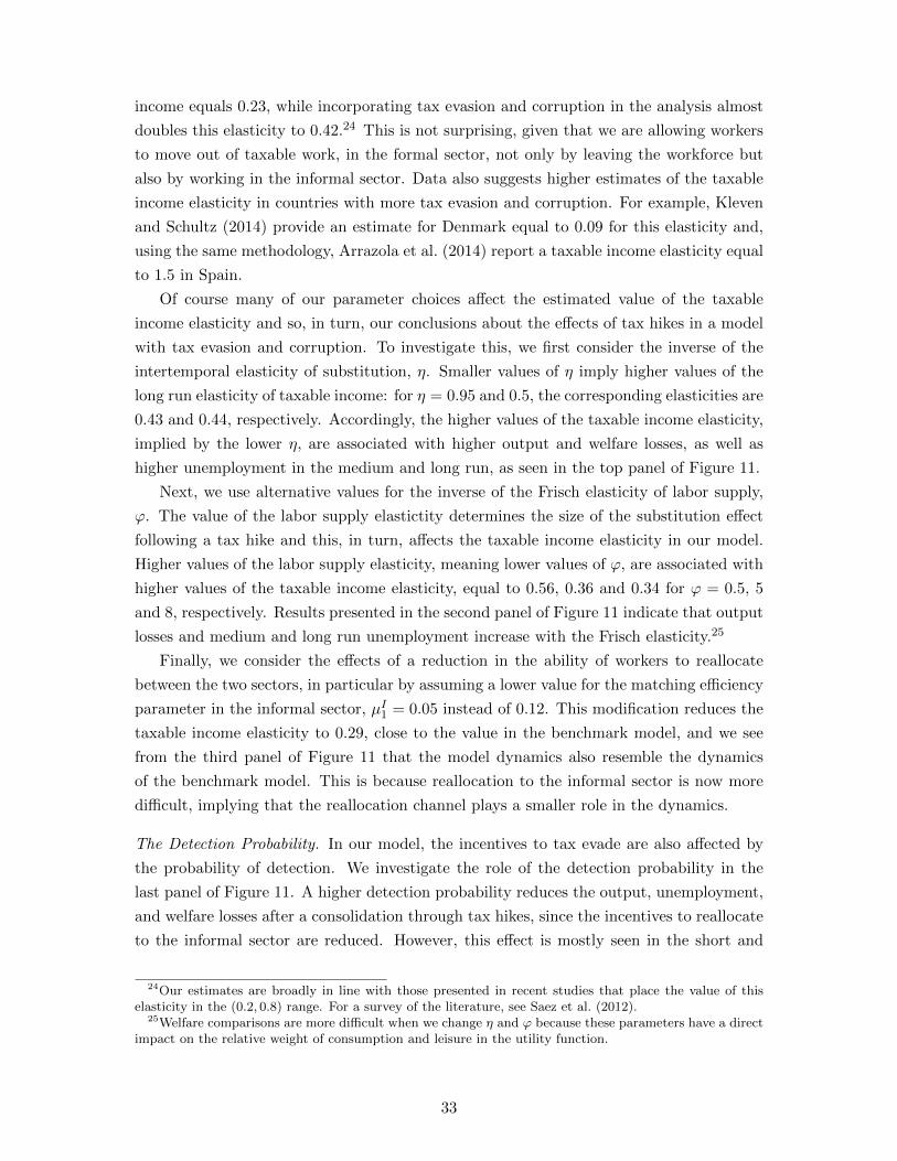
income equals 0.23, while incorporating tax evasion and corruption in the analysis almost

doubles this elasticity to 0.42.24 This is not surprising, given that we are allowing workers

to move out of taxable work, in the formal sector, not only by leaving the workforce but

also by working in the informal sector. Data also suggests higher estimates of the taxable

income elasticity in countries with more tax evasion and corruption. For example, Kleven

and Schultz (2014) provide an estimate for Denmark equal to 0.09 for this elasticity and,

using the same methodology, Arrazola et al. (2014) report a taxable income elasticity equal

to 1.5 in Spain.

Of course many of our parameter choices affect the estimated value of the taxable

income elasticity and so, in turn, our conclusions about the effects of tax hikes in a model

with tax evasion and corruption. To investigate this, we first consider the inverse of the

intertemporal elasticity of substitution, η. Smaller values of η imply higher values of the

long run elasticity of taxable income: for η = 0.95 and 0.5, the corresponding elasticities are

0.43 and 0.44, respectively. Accordingly, the higher values of the taxable income elasticity,

implied by the lower η, are associated with higher output and welfare losses, as well as

higher unemployment in the medium and long run, as seen in the top panel of Figure 11.

Next, we use alternative values for the inverse of the Frisch elasticity of labor supply,

ϕ. The value of the labor supply elastictity determines the size of the substitution effect

following a tax hike and this, in turn, affects the taxable income elasticity in our model.

Higher values of the labor supply elasticity, meaning lower values of ϕ, are associated with

higher values of the taxable income elasticity, equal to 0.56, 0.36 and 0.34 for ϕ = 0.5, 5

and 8, respectively. Results presented in the second panel of Figure 11 indicate that output

losses and medium and long run unemployment increase with the Frisch elasticity.25

Finally, we consider the effects of a reduction in the ability of workers to reallocate

between the two sectors, in particular by assuming a lower value for the matching efficiency

parameter in the informal sector, µI1 = 0.05 instead of 0.12. This modification reduces the

taxable income elasticity to 0.29, close to the value in the benchmark model, and we see

from the third panel of Figure 11 that the model dynamics also resemble the dynamics

of the benchmark model. This is because reallocation to the informal sector is now more

difficult, implying that the reallocation channel plays a smaller role in the dynamics.

The Detection Probability. In our model, the incentives to tax evade are also affected by

the probability of detection. We investigate the role of the detection probability in the

last panel of Figure 11. A higher detection probability reduces the output, unemployment,

and welfare losses after a consolidation through tax hikes, since the incentives to reallocate

to the informal sector are reduced. However, this effect is mostly seen in the short and

24Our estimates are broadly in line with those presented in recent studies that place the value of thiselasticity in the (0.2, 0.8) range. For a survey of the literature, see Saez et al. (2012).

25Welfare comparisons are more difficult when we change η and ϕ because these parameters have a directimpact on the relative weight of consumption and leisure in the utility function.

33

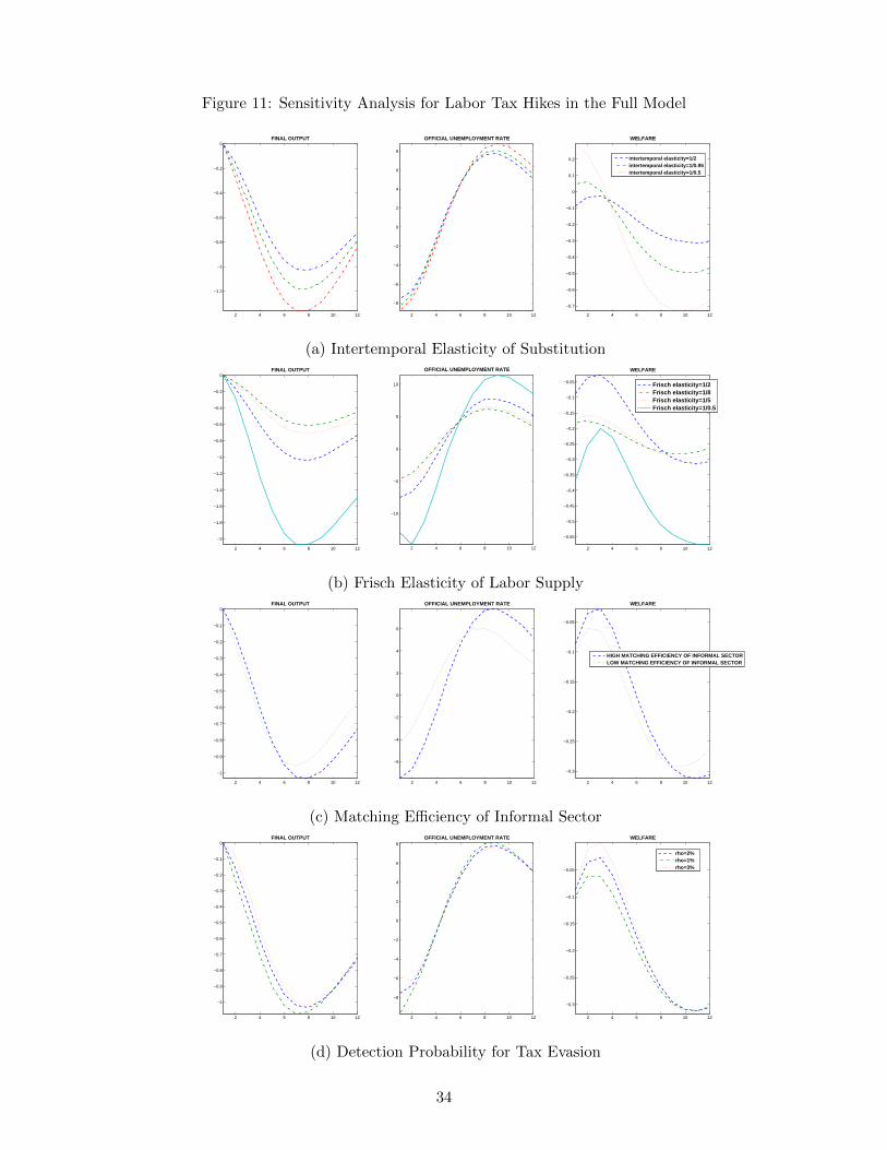
Figure 11: Sensitivity Analysis for Labor Tax Hikes in the Full Model

2 4 6 8 10 12

−1.2

−1

−0.8

−0.6

−0.4

−0.2

0FINAL OUTPUT

2 4 6 8 10 12

−8

−6

−4

−2

0

2

4

6

8

OFFICIAL UNEMPLOYMENT RATE

2 4 6 8 10 12

−0.7

−0.6

−0.5

−0.4

−0.3

−0.2

−0.1

0

0.1

0.2

WELFARE

intertemporal elasticity=1/2intertemporal elasticity=1/0.95intertemporal elasticity=1/0.5

(a) Intertemporal Elasticity of Substitution

2 4 6 8 10 12

−2

−1.8

−1.6

−1.4

−1.2

−1

−0.8

−0.6

−0.4

−0.2

0FINAL OUTPUT

2 4 6 8 10 12

−10

−5

0

5

10

OFFICIAL UNEMPLOYMENT RATE

2 4 6 8 10 12

−0.55

−0.5

−0.45

−0.4

−0.35

−0.3

−0.25

−0.2

−0.15

−0.1

−0.05

WELFARE

Frisch elasticity=1/2 Frisch elasticity=1/8Frisch elasticity=1/5Frisch elasticity=1/0.5

(b) Frisch Elasticity of Labor Supply

2 4 6 8 10 12

−1

−0.9

−0.8

−0.7

−0.6

−0.5

−0.4

−0.3

−0.2

−0.1

0FINAL OUTPUT

2 4 6 8 10 12

−6

−4

−2

0

2

4

6

OFFICIAL UNEMPLOYMENT RATE

2 4 6 8 10 12

−0.3

−0.25

−0.2

−0.15

−0.1

−0.05

WELFARE

HIGH MATCHING EFFICIENCY OF INFORMAL SECTORLOW MATCHING EFFICIENCY OF INFORMAL SECTOR

(c) Matching Efficiency of Informal Sector

2 4 6 8 10 12

−1

−0.9

−0.8

−0.7

−0.6

−0.5

−0.4

−0.3

−0.2

−0.1

0FINAL OUTPUT

2 4 6 8 10 12

−8

−6

−4

−2

0

2

4

6

8OFFICIAL UNEMPLOYMENT RATE

2 4 6 8 10 12

−0.3

−0.25

−0.2

−0.15

−0.1

−0.05

WELFARE

rho=2%rho=1%rho=3%

(d) Detection Probability for Tax Evasion

34

medium run; in the long run, the results are similar for the different values of ρ.26

5. Policy Evaluation

Since the model qualitatively replicates the empirical evidence presented in Section 2,

we employ it to evaluate the effects of consolidation packages implemented in southern

European countries in recent years. We recalibrate the model for Greece, Portugal and

Spain, three countries which are also characterized by high corruption and tax evasion,

and analyze the effects of their recent consolidation packages.

5.1. Calibration

Using the information in OECD (2012), we adjust the size of the consolidation in each

country to match the reduction in the deficit-to-GDP ratio implemented in 2010 and also

replicate the announced consolidation volumes in the long run. Table 5 reports the consoli-

dation in 2010 for each country and the intended consolidation to be implemented by 2015.

We see that Greece implemented the most severe austerity package. The consolidation

package of Italy in 2010 was small, but larger consolidation volumes were announced for

2015. The consolidation packages in Spain and Portugal were similar in 2010, but Portu-

gal announced a slightly larger long run consolidation volume. In order to replicate the

actual consolidation packages, we allow both instruments to move simultaneously, again

using OECD (2012) to fix the relative contribution of the two instruments for each coun-

try. Portugal used more tax hikes than expenditure cuts, while the other countries used

predominantly expenditure-based measures.27

Table 5 also summarizes the differences in the calibration for the various economies. We

use the estimates of shadow output in Elgin and Oztunah (2012) to determine the relative

share of shadow employment across countries, which gives comparable numbers, though

slightly higher in Greece. Following the World Bank’s Control of Corruption index, shown

in Figure 1, we set the embezzlement rate in Greece and Italy higher than Spain and Portu-

gal. According to the OECD statistics, Portugal has a notably healthier labor market, with

the highest labor force participation rate and the lowest unemployment rate. According to

the CEP-OECD database and the ICTWSS (Data Base on Institutional Characteristics of

Trade Unions, Wage Setting, State Intervention and Social Pacts, 1960-2011) indices, Italy

and Greece have higher unionisation and coordination of bargaining, reflected in our model

by lower bargaining power for firms, compared to Spain and Portugal. Also, according to

the CEP-OECD database and the estimates in Martin (1996), replacement rates are lower

in Italy and Greece relative to Spain and Portugal. Accordingly in Table 5 we assume

replacement rates of 35% for Italy and Greece and 45% for Portugal and Spain. Spain

26Since the auditing probability affects the reallocation of workers between sectors, it could also affect theconsolidation through spending cuts. However, the results under the alternative values of ρ do not changesubstantially compared to the results of the baseline calibration.

27See the tables on p.138, 166, 206, 226 of OECD (2012).

35

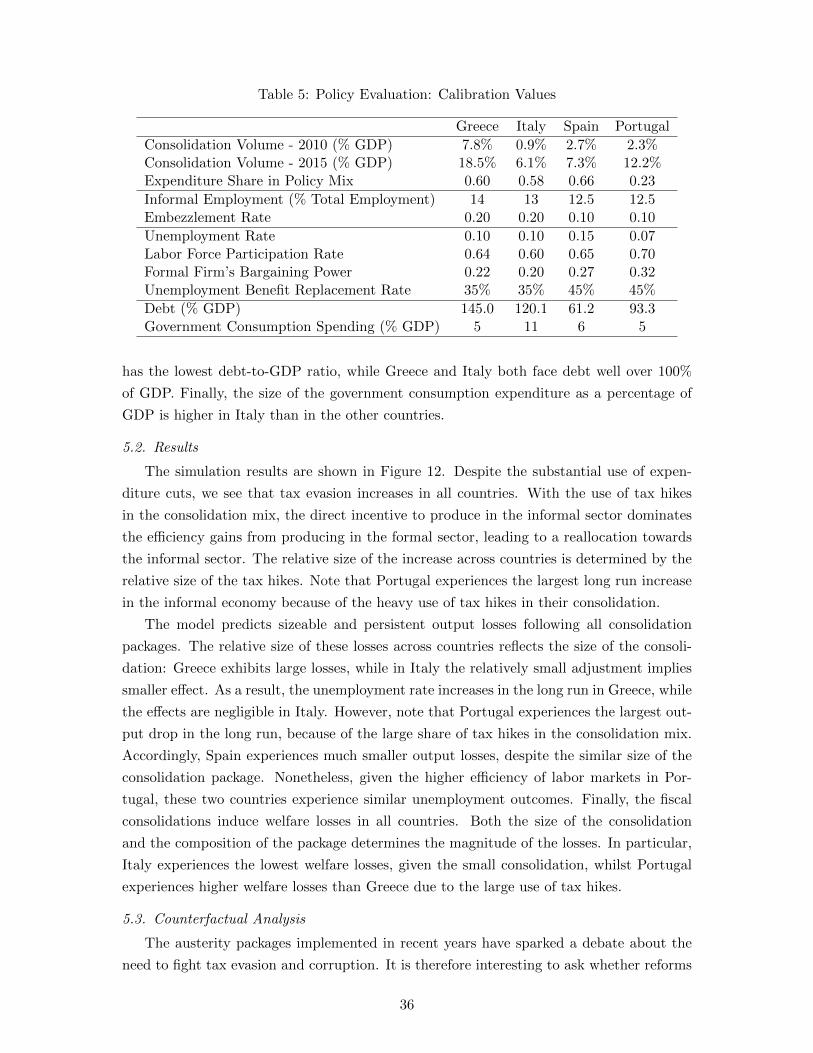
Table 5: Policy Evaluation: Calibration Values

Greece Italy Spain Portugal

Consolidation Volume - 2010 (% GDP) 7.8% 0.9% 2.7% 2.3%Consolidation Volume - 2015 (% GDP) 18.5% 6.1% 7.3% 12.2%Expenditure Share in Policy Mix 0.60 0.58 0.66 0.23

Informal Employment (% Total Employment) 14 13 12.5 12.5Embezzlement Rate 0.20 0.20 0.10 0.10

Unemployment Rate 0.10 0.10 0.15 0.07Labor Force Participation Rate 0.64 0.60 0.65 0.70Formal Firm’s Bargaining Power 0.22 0.20 0.27 0.32Unemployment Benefit Replacement Rate 35% 35% 45% 45%

Debt (% GDP) 145.0 120.1 61.2 93.3Government Consumption Spending (% GDP) 5 11 6 5

has the lowest debt-to-GDP ratio, while Greece and Italy both face debt well over 100%

of GDP. Finally, the size of the government consumption expenditure as a percentage of

GDP is higher in Italy than in the other countries.

5.2. Results

The simulation results are shown in Figure 12. Despite the substantial use of expen-

diture cuts, we see that tax evasion increases in all countries. With the use of tax hikes

in the consolidation mix, the direct incentive to produce in the informal sector dominates

the efficiency gains from producing in the formal sector, leading to a reallocation towards

the informal sector. The relative size of the increase across countries is determined by the

relative size of the tax hikes. Note that Portugal experiences the largest long run increase

in the informal economy because of the heavy use of tax hikes in their consolidation.

The model predicts sizeable and persistent output losses following all consolidation

packages. The relative size of these losses across countries reflects the size of the consoli-

dation: Greece exhibits large losses, while in Italy the relatively small adjustment implies

smaller effect. As a result, the unemployment rate increases in the long run in Greece, while

the effects are negligible in Italy. However, note that Portugal experiences the largest out-

put drop in the long run, because of the large share of tax hikes in the consolidation mix.

Accordingly, Spain experiences much smaller output losses, despite the similar size of the

consolidation package. Nonetheless, given the higher efficiency of labor markets in Por-

tugal, these two countries experience similar unemployment outcomes. Finally, the fiscal

consolidations induce welfare losses in all countries. Both the size of the consolidation

and the composition of the package determines the magnitude of the losses. In particular,

Italy experiences the lowest welfare losses, given the small consolidation, whilst Portugal

experiences higher welfare losses than Greece due to the large use of tax hikes.

5.3. Counterfactual Analysis

The austerity packages implemented in recent years have sparked a debate about the

need to fight tax evasion and corruption. It is therefore interesting to ask whether reforms

36

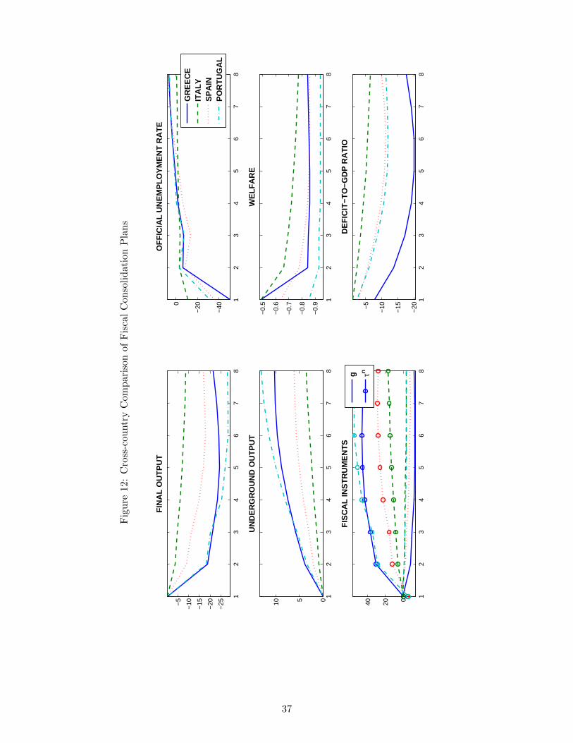
Fig

ure

12:

Cro

ss-c

ountr

yC

omp

aris

onof

Fis

cal

Con

soli

dat

ion

Pla

ns

12

34

56

78

−25

−20

−15

−10−

5

FIN

AL

OU

TP

UT

12

34

56

78

−40

−200

OF

FIC

IAL

UN

EM

PLO

YM

EN

T R

AT

E

12

34

56

78

0510

UN

DE

RG

RO

UN

D O

UT

PU

T

12

34

56

78

−0.

9

−0.

8

−0.

7

−0.

6

−0.

5

WE

LFA

RE

12

34

56

78

02040

FIS

CA

L IN

ST

RU

ME

NT

S

12

34

56

78

−20

−15

−10−

5

DE

FIC

IT−T

O−G

DP

RA

TIO

g τn

GR

EE

CE

ITA

LYS

PA

INP

OR

TU

GA

L

37

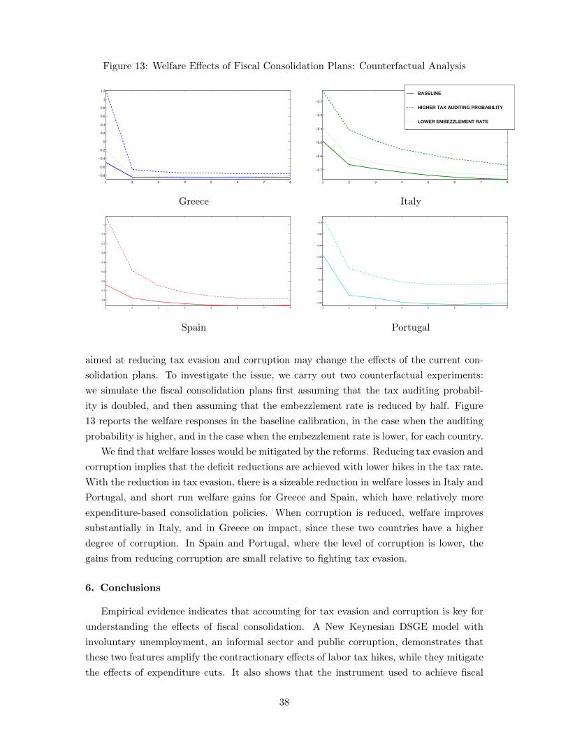
Figure 13: Welfare Effects of Fiscal Consolidation Plans: Counterfactual Analysis

1 2 3 4 5 6 7 8

−0.8

−0.6

−0.4

−0.2

0

0.2

0.4

0.6

0.8

1

1.2

1 2 3 4 5 6 7 8

−0.7

−0.6

−0.5

−0.4

−0.3

−0.2

BASELINE

HIGHER TAX AUDITING PROBABILITY

LOWER EMBEZZLEMENT RATE

Greece Italy

1 2 3 4 5 6 7 8

−0.8

−0.7

−0.6

−0.5

−0.4

−0.3

−0.2

−0.1

0

1 2 3 4 5 6 7 8

−0.94

−0.92

−0.9

−0.88

−0.86

−0.84

−0.82

−0.8

Spain Portugal

aimed at reducing tax evasion and corruption may change the effects of the current con-

solidation plans. To investigate the issue, we carry out two counterfactual experiments:

we simulate the fiscal consolidation plans first assuming that the tax auditing probabil-

ity is doubled, and then assuming that the embezzlement rate is reduced by half. Figure

13 reports the welfare responses in the baseline calibration, in the case when the auditing

probability is higher, and in the case when the embezzlement rate is lower, for each country.

We find that welfare losses would be mitigated by the reforms. Reducing tax evasion and

corruption implies that the deficit reductions are achieved with lower hikes in the tax rate.

With the reduction in tax evasion, there is a sizeable reduction in welfare losses in Italy and

Portugal, and short run welfare gains for Greece and Spain, which have relatively more

expenditure-based consolidation policies. When corruption is reduced, welfare improves

substantially in Italy, and in Greece on impact, since these two countries have a higher

degree of corruption. In Spain and Portugal, where the level of corruption is lower, the

gains from reducing corruption are small relative to fighting tax evasion.

6. Conclusions

Empirical evidence indicates that accounting for tax evasion and corruption is key for

understanding the effects of fiscal consolidation. A New Keynesian DSGE model with

involuntary unemployment, an informal sector and public corruption, demonstrates that

these two features amplify the contractionary effects of labor tax hikes, while they mitigate

the effects of expenditure cuts. It also shows that the instrument used to achieve fiscal

38

consolidation affects the incentives of agents to produce in the informal sector. Consistent

with VAR evidence obtained for Italian, spending cuts reduce the size of the informal

economy, while tax hikes increase it.

Given the model’s ability to reproduce the qualitative features of the data, we ana-

lyze how current fiscal consolidation plans in Greece, Italy, Portugal and Spain affect tax

evasion, output, unemployment and welfare. The model predicts increasing levels of tax

evasion during the consolidation in all countries, and prolonged output and welfare losses.

Greece suffers heavy losses due to the severity of the austerity package implemented; Por-

tugal experiences the largest drops in output and welfare because of the heavy use of tax

hikes in their consolidation package. Furthermore, the welfare costs of these consolidations

would have been smaller if tax evasion and corruption had been reduced. Hence, reforms

aimed at fighting public corruption and tax evasion should go hand-in-hand with austerity

measures in order to mitigate the welfare costs of fiscal consolidations.

Our exercise is the first attempt to analyze the effects of fiscal consolidation in the

presence of tax evasion and corruption. Since the model is stylized, it leaves out important

aspects of reality that could affect our conclusions. For example, in our economy there is a

representative household, and so we cannot assess the effects of tax evasion and corruption

on income inequality. Also, we consider only cuts in government consumption expenditures

and not in other items of the government budget. Furthermore, our model does not allow

for evasion of consumption taxes, which is an important component of tax evasion in

southern European countries. Finally, the model treats the degree of public corruption as

a parameter, which does not allow it to respond to cyclical factors or to interact with tax

evasion. We leave these extensions for future research.

39

[1] Alesina A. and S. Ardagna, 2010, ‘Large Changes in Fiscal Policy: Taxes versus

Spending’, NBER Chapters, Tax Policy and the Economy, 24, 35-68.

[2] Alesina A., C. Favero and F. Giavazzi, 2013, ‘The Output Effect of Fiscal Consolida-

tions’, Working Papers 478, IGIER, Bocconi University.

[3] Ardizzi G., C. Petraglia, M. Piacenza and G. Tutati, 2012, ‘Measuring the Under-

ground Economy with the Currency Demand Approach: A Reinterpretation of the

Methodology, with an Application to Italy’, Bank of Italy Working Paper Series, No.

864.

[4] Arrazola, M., J. de Hevia, D. Romero and J. F. Sanz-Sanz, 2014, ‘Personal Income Tax

Reforms and the Elasticity of Reported Income to Marginal Tax Rates: An Empirical

Analysis Applied to Spain’, Victoria University of Wellington Chair in Public Finance

Working Paper Series 3593.

[5] Bermperoglou D., E. Pappa and E. Vella, 2014, ‘Spending Cuts and Their Effects on

Output, Unemployment and the Deficit’, Unpublished Manuscript.

[6] Blanchard, O. and D. Leigh, 2013, ‘Growth Forecast Errors and Fiscal Multipliers’,

IMF Working Papers 13/1.

[7] Boeri T. and P. Garibaldi, 2007, ‘Shadow Sorting,’ NBER International Seminar on

Macroeconomics 2005, MIT Press, 125-163.

[8] Bruckner, M. and E. Pappa, 2012, ‘Fiscal Expansions, Unemployment, and Labor

Force Participation: Theory and Evidence’, International Economic Review, 53(4),

1205-1228.

[9] Buehn A. and F. Schneider, 2012, ‘Corruption and the Shadow Economy: Like Oil

and Vinegar, Like Water and Fire?’, International Tax and Public Finance, 19(1),

172-194.

[10] Busato F. and B. Chiarini, 2004, ‘Market and Underground Activities in a Two-Sector

Dynamic Equilibrium Model’, Economic Theory, 23(4), 831-861.

[11] Calvo, G. A., 1983, ‘Staggered Prices in a Utility-Maximizing Framework,’ Journal of

Monetary Economics, 12(3), 383-398.

[12] Campolmi A. and S. Gnocchi, 2014, ‘Labor Market Participation, Unemployment and

Monetary Policy’, Bank of Canada Working Paper No. 2014/9.

[13] Charron N., V. Lapuente and L. Dijkstra, 2012, ‘Regional Governance Matters: A

Study on the Regional Variation in Quality of Government within the EU’, European

Commission Working Paper Series No. 01/2012.

40

[14] Colombo E., L. Onnis and P. Tirelli, 2014, ‘Shadow Economies at Times of Banking

Crises: Empirics and Theory’, Journal of Banking and Finance, forthcoming.

[15] Devries, P., J. Guajardo, D. Leigh and A. Pescatori, 2011, ‘A New Action-based

Dataset of Fiscal Consolidation’, IMF Working Papers 11/128

[16] Elgin C. and O. Oztunah O., 2012, ‘Shadow Economies Around the World: Model

Based Estimates’, working paper.

[17] Erceg, C. and J. Linde, 2013, ‘Fiscal Consolidation in a Currency Union: Spending

Cuts vs. Tax Hikes,’ Journal of Economic Dynamics and Control, 37(2), 422-445.

[18] Feldstein, M., 1999, Tax Avoidance and the Deadweight Loss of the Income Tax,

Review of Economics and Statistics, 81(4), 674-680.

[19] Fugazza M. and J.-F. Jacques, 2004, ‘Labor Market Institutions, Taxation and the

Underground Economy,’ Journal of Public Economics, 88, 395-418.

[20] Galı, J., J. D. Lopez-Salido and J. Valles, 2007, ‘Understanding the Effects of Gov-

ernment Spending on Consumption,’ Journal of the European Economic Association,

5(1), 227-270.

[21] Gallagher, M., 1991, ‘Rent-Seeking and Economic Growth in Africa’, Westview Press.

[22] Gestha, 2014, ‘La Economıa Sumergida Pasa Factura. El Avance del Fraude en Espana

Durante la Crisis’, Madrid, enero de 2014.

[23] Hansen G., 1985, ‘Indivisible Labor and the Business Cycle,’ Journal of Monetary

Economics, 16, 309-27.

[24] Hansen L. P., and K. Singleton, 1983, ‘Stochastic Consumption, Risk Aversion and

the Temporal Behavior of Asset Returns’, Journal of Political Economy, 91, 249-265.

[25] ISTAT, 2010, ‘La Misura dell’Economia Sommersa Secondo le Statistiche Ufficialli.

Anni 2000-2008,’ Conti-Nazionali-Statistiche in Breve, Istituto Nazionale di Statistica,

Rome.

[26] Kleven, H. and E. Schultz, 2014, ‘Estimating Taxable Income Responses Using Danish

Tax Reforms’, American Economic Journal: Economic Policy, forthcoming.

[27] Krueger, A., 1974, ‘The Political Economy of the Rent-Seeking Society’, The American

Economic Review, 64(3), 291-303.

[28] Martin J., 1996, ‘Measures of Replacement Rates for the Purpose of International

Comparison: A Note’, OECD Economic Studies, 26(1), 98-118.

[29] Martin, P. and T. Philippon, 2014, ‘Inspecting the Mechanism: Leverage and the

Great Recession in the Eurozone,’ Unpublished Manuscript.

41

[30] OECD, 2012, Restoring Public Finances, 2012 Update, OECD Publishing.

http://dx.doi.org/10.1787/9789264179455-en

[31] Orsi R., D. Raggi and F. Turino, 2014, ‘Size, Trend, and Policy Implications of the

Underground Economy’, forthcoming in the Review of Economic Dynamics.

[32] Pappada, F. and Y. Zylberberg, 2014, ‘Austerity Plans and Tax Evasion: Theory and

Evidence from Greece’, Unpublished Manuscript.

[33] Peracchi F. and E. Viviano, 2004, ‘An Empirical Micro Matching Model with an

Application to Italy and Spain’, Temi di discussione No. 538, Banca d Italia.

[34] Perotti, R., 1996, ‘Fiscal Consolidation in the Europe: Composition Matters’, Amer-

ican Economic Review Papers and Proceedings, 86(2), 105-110.

[35] Perotti, R., 2005, ‘Estimating the Effects of Fiscal Policy in OECD Countries’, Pro-

ceedings, Federal Reserve Bank of San Francisco.

[36] Ravn, M. O., 2008, ‘The Consumption-Tightness Puzzle’, NBER Chapters, NBER

International Seminar on Macroeconomics 2006, 9-63.

[37] Restrepo-Echavarria P., 2014, ‘Macroeconomic Volatility: The Role of the Informal

Economy,’ European Economic Review, 70, 454-469.

[38] Saez, E., J. Slemrod, and S. H. Giertz, 2012, ‘The Elasticity of Taxable Income with

Respect to Marginal Tax Rates: A Critical Review’, Journal of Economic Literature,

50(1), 3-50.

[39] Schneider F. and A. Buehn, 2012, ‘Shadow Economies in Highly Developed OECD

Countries: What are the Driving Forces?’, IZA discussion paper No. 6891, Institute

for the study of labor, University of Bonn, Bonn, 2012.

42