FIRST YEAR WILKINSON MICROWAVE ANISOTROPY PROBE (WMAP1)OBSERVATIONS: IMPLICATIONS FOR INFLATION

H. V. Peiris2, E. Komatsu2, L. Verde2 � 3, D. N. Spergel2, C. L. Bennett4, M. Halpern5, G. Hinshaw4, N. Jarosik6, A. Kogut4, M. Limon4 � 7, S. S. Meyer8, L. Page6, G. S. Tucker4 � 7 � 9, E. Wollack4, E.

L. Wright10

hiranya@astro.princeton.edu

ABSTRACT

We confront predictions of inflationary scenarios with the WMAP data, in com-bination with complementary small-scale CMB measurements and large-scale struc-ture data. The WMAP detection of a large-angle anti-correlation in the temperature–polarization cross-power spectrum is the signature of adiabatic superhorizon fluctu-ations at the time of decoupling. The WMAP data are described by pure adiabaticfluctuations: we place an upper limit on a correlated CDM isocurvature component.Using WMAP constraints on the shape of the scalar power spectrum and the ampli-tude of gravity waves, we explore the parameter space of inflationary models thatis consistent with the data. We place limits on inflationary models; for example, aminimally-coupled

��� 4 is disfavored at more than 3- � using WMAP data in com-bination with smaller scale CMB and large scale structure survey data. The limitson the primordial parameters using WMAP data alone are: ns(k0 = 0 � 002 Mpc−1) =1 � 20+0 � 12

−0 � 11, dns � d lnk= −0 � 077+0 � 050−0 � 052, A(k0 = 0 � 002 Mpc−1) = 0 � 71+0 � 10

−0 � 11 (68% CL), andr(k0 = 0 � 002 Mpc−1) � 1 � 28 (95% CL).

1WMAP is the result of a partnership between Princeton University and NASA’s Goddard Space Flight Center.Scientific guidance is provided by the WMAP Science Team.

2Dept of Astrophysical Sciences, Princeton University, Princeton, NJ 08544

3Chandra Fellow

4Code 685, Goddard Space Flight Center, Greenbelt, MD 20771

5Dept. of Physics and Astronomy, University of British Columbia, Vancouver, BC Canada V6T 1Z1

6Dept. of Physics, Jadwin Hall, Princeton, NJ 08544

7National Research Council (NRC) Fellow

8Depts. of Astrophysics and Physics, EFI and CfCP, University of Chicago, Chicago, IL 60637

9Dept. of Physics, Brown University, Providence, RI 02912

10UCLA Astronomy, PO Box 951562, Los Angeles, CA 90095-1562

– 2 –

Subject headings: cosmic microwave background — cosmology: observations —early universe

1. INTRODUCTION

An epoch of accelerated expansion in the early universe, inflation, dynamically resolves cos-mological puzzles such as homogeneity, isotropy, and flatness of the universe (Guth 1981; Linde1982; Albrecht & Steinhardt 1982; Sato 1981), and generates superhorizon fluctuations without ap-pealing to fine-tuned initial setups (Mukhanov & Chibisov 1981; Hawking 1982; Guth & Pi 1982;Starobinsky 1982; Bardeen et al. 1983; Mukhanov et al. 1992). During the accelerated expan-sion phase, generation and amplification of quantum fluctuations in scalar fields are unavoidable(Parker 1969; Birrell & Davies 1982). These fluctuations become classical after crossing the eventhorizon. Later during the deceleration phase they re-enter the horizon, and seed the matter and theradiation fluctuations observed in the universe.

The majority of inflation models predict Gaussian, adiabatic, nearly scale-invariant primor-dial fluctuations. These properties are generic predictions of inflationary models. The cosmic mi-crowave background (CMB) radiation anisotropy is a promising tool for testing these properties,as the linearity of the CMB anisotropy preserves basic properties of the primordial fluctuations. Incompanion papers, Spergel et al. (2003) find that adiabatic scale-invariant primordial fluctuationsfit the WMAP CMB data as well as a host of other astronomical data sets including the galaxy andthe Lyman- � power spectra; Komatsu et al. (2003) find that the WMAP CMB data is consistentwith Gaussian primordial fluctuations. These results indicate that predictions of the most basicinflationary models are in good agreement with the data.

While the inflation paradigm has been very successful, radically different inflationary modelsyield similar predictions for the properties of fluctuations: Gaussianity, adiabaticity, and near-scale-invariance. To break the degeneracy among the models, we need to measure the primordialfluctuations precisely. Even a slight deviation from Gaussian, adiabatic, near-scale-invariant fluc-tuations can place strong constraints on the models (Liddle & Lyth 2000). The CMB anisotropyarising from primordial gravitational waves can also be a powerful method for model testing. Inthis paper, we confront predictions of various inflationary models with the CMB data from theWMAP, CBI (Pearson et al. 2002), and ACBAR (Kuo et al. 2002) experiments, as well as the2dFGRS (Percival et al. 2001) and Lyman- � power spectra (Croft et al. 2002; Gnedin & Hamilton2002).

This paper is organized as follows. In § 2, we show that the WMAP detection of an anti-correlation between the temperature and the polarization fluctuations at l � 150 is the distinctive

– 3 –

signature of adiabatic superhorizon fluctuations. We compare the data with specific predictions ofinflationary models: single-field models in § 3, and double-field models in § 4. We examine theevidence for features in the inflaton potential in § 5. Finally, we summarize our results and drawconclusions in § 6.

2. IMPLICATIONS OF WMAP “TE” DETECTION FOR THE INFLATIONARYPARADIGM

A fundamental feature of inflationary models is a period of accelerated expansion in the veryearly universe. During this time, quantum fluctuations are highly amplified, and their wavelengthsare stretched to outside the Hubble horizon. Thus, the generation of large-scale fluctuations is aninevitable feature of inflation. These fluctuations are coherent on what appear to be superhorizonscales at decoupling. Without accelerated expansion, the causal horizon at decoupling is � 2degrees. Causality implies that the correlation length scale for fluctuations can be no larger thanthis scale. Thus, the detection of superhorizon fluctuations is a distinctive signature of this earlyepoch of acceleration.

The COBE DMR detection of large scale fluctuations has been sometimes described as adetection of superhorizon scale fluctuations. While this is the most likely interpretation of theCOBE results, it is not unique. There are several possible mechanisms for generating large-scaletemperature fluctuations. For example, texture models predict a nearly scale-invariant spectrum oftemperature fluctuations on large angular scales (Pen et al. 1994). The COBE detection sounded thedeath knell for these particular models not through its detection of fluctuations, but due to the lowamplitude of the observed fluctuations. The detection of acoustic temperature fluctuations is alsosometimes evoked as the definitive signature of superhorizon scale fluctuations (Hu & White 1997).String and defect models do not produce sharp acoustic peaks (Albrecht et al. 1996; Turok et al.1998). However, the detection of acoustic peaks in the temperature angular power spectrum doesnot prove that the fluctuations are superhorizon, as causal sources acting purely through gravitycan exactly mimic the observed peak pattern (Turok 1996a,b). The recent study of causal seedmodels by Durrer et al. (2002) shows that they can reproduce much of the observed peak structureand provide a plausible fit to the pre-WMAP CMB data.

The large-angle (50�

l�

150) temperature-polarization anti-correlation detected by WMAP(Kogut et al. 2003) is a distinctive signature of superhorizon adiabatic fluctuations (Spergel &Zaldarriaga 1997). The reason for this conclusion is explained as follows. Throughout this section,we consider only scales larger than the sound horizon at the decoupling epoch. Zaldarriaga &Harari (1995) show that, in the tight coupling approximation, the polarization signal arises from

– 4 –

the gradient of the peculiar velocity of the photon fluid, � 1,�E � −0 � 17(1 − � 2)

���deck � 1(

�dec) � (1)

where�

E is the E-mode (parity-even) polarization fluctuation,�

dec is the conformal time at decou-pling,

���dec is the thickness of the surface of last scattering in conformal time, and � = cos(

�k � �n).

The velocity gradient generates a quadrupole temperature anisotropy pattern around electronswhich, in turn, produces the E-mode polarization. Note that while reionization violates the assump-tions of tight coupling, the existence of clear acoustic oscillations in the temperature-polarization(TE) and temperature-temperature (TT) angular power spectra imply that most ( � 85%) CMB pho-tons detected by WMAP did indeed come from z = 1089 where the tight coupling approximationis valid. The velocity � 1 is related to the photon density fluctuations, � 0, through the continuity

equation, k � 1 = −3�� 0 +

�� , where

�is Bardeen’s curvature perturbation. The observable tem-

perature fluctuations on large scales are approximately given by�

T = � 0(�

dec) + � (�

dec), where� is the Newtonian potential, which equals −�

in the absence of anisotropic stress. Therefore,roughly speaking, the photon density fluctuations generate temperature fluctuations, while the ve-locity gradient generates polarization fluctuations.

The tight coupling approximation implies that the baryon photon fluid is governed by a singlesecond-order differential equation which yields a series of acoustic peaks (Peebles & Yu 1970; Hu& Sugiyama 1995):

( �� 0 + �� ) +

aa

R1 + R

(� 0 +

�) + k2c2

s ( � 0 +�

) = k2 � c2s

�−�3 � � (2)

where the sound speed cs is given by c2s = [3(1 + R)]−1. The large-scale solution to this equation is

(Hu & Sugiyama 1995)

� 0(�) +�

(�) = [ � 0(0) +

�(0)]cos(kcs

�) + kcs ���

0d����� �

(���

) − � (���

) � sin[kcs(�

−���

)] � (3)

and the continuity equation gives the solution for the peculiar velocity,

13cs� 1(

�) = [ � 0(0) +

�(0)]sin(kcs

�) − kcs � �

0d����� �

(���

) − � (���

) � cos[kcs(�

−���

)] � (4)

These solutions (equations (1), (3), and (4)) are valid regardless of the nature of the source offluctuations.

In inflationary models, a period of accelerated expansion generates superhorizon adiabaticfluctuations, so that the first term in equation (3) and (4) is non-zero. Since � � −

�and � 0(0) +�

(0) = 32

�(0) = 5

3

�(�

dec) on superhorizon scales, one obtains�

T � − 13

�(�

dec)cos(kcs�

dec), and

– 5 –�E � 0 � 17(1 − � 2)kcs

���dec�

(�

dec) sin(kcs�

dec) (see Hu & Sugiyama (1995) and Zaldarriaga &Harari (1995) for derivation). Therefore, the cross correlation is found to be

� �T�

E � � −0 � 03(1 − � 2)(kcs���

dec)P� (k) sin(2kcs�

dec) � (5)

where P� (k) is the power spectrum of�

(�

dec). The observable correlation function is estimated ask3� �

T�

E � . Clearly, there is an anti-correlation peak near kcs�

dec � 3 � � 4, which corresponds tol � 150: this is the distinctive signature of primordial adiabatic fluctuations. In other words, theanti-correlation appears on superhorizon scales at decoupling, because of the modulation betweenthe density mode, cos(kcs

�dec), and the velocity mode, sin(kcs

�dec), yielding sin(2kcs

�dec), which

has a peak on scales larger than the horizon size, c�

dec ��� 3cs�

dec.

Cosmic strings and textures are examples of active models. In these models, causal fielddynamics continuously generate spatial variations in the energy density of a field. Magueijo et al.(1996) describe the general dynamics of active models. These models do not have the first term inequation (3) and (4), but the fluctuations are produced by the second term, the growth of

�and � .

The same applies to primordial isocurvature fluctuations, where the non-adiabatic pressure causes�and � to grow. While the problem is more complicated, these models give a positive correlation

between temperature and polarization fluctuations on large scales. This positive correlation ispredicted not just for texture (Seljak et al. 1997) and scaling seed models (Durrer et al. 2002), butis the generic signature of any causal models (Hu & White 1997)11 that lack a period of acceleratedexpansion.

Figure 1 shows the predictions of the TE large angle correlation predicted in typical primordialadiabatic, isocurvature, and causal scaling seed models compared with the WMAP data. The causalscaling seed model shown is a flat Family I model in the classification of Durrer et al. (2002) thatprovided a good fit to the pre-WMAP temperature data.

The WMAP detection of a TE anti-correlation at l � 50 − 150, scales that correspond to su-perhorizon scales at the epoch of decoupling, rules out a broad class of active models. It impliesthe existence of superhorizon, adiabatic fluctuations at decoupling. If these fluctuations were gen-erated dynamically rather than by setting special initial conditions then the TE detection requiresthat the universe had a period of accelerated expansion. In addition to inflation, the pre-Big-Bangscenario (Gasperini & Veneziano 1993) and the Ekpyrotic scenario (Khoury et al. 2001, 2002)predict the existence of superhorizon fluctuations.

11Hu & White (1997) use an opposite sign convention for the TE cross power spectrum.

– 6 –

3. SINGLE FIELD INFLATION MODELS

In this section we explore how predictions of specific models that implement inflation (seeLyth & Riotto (1999) for a survey) compare with current observations.

3.1. Introduction

The definition of “single-field inflation” encompasses the class of models in which the infla-tionary epoch is described by a single scalar field, the inflaton field. We also include a class ofmodels called “hybrid” inflation models as single-field models. While hybrid inflation requires asecond field to end inflation (Linde 1994), the second field does not contribute to the dynamicsof inflation or the observed fluctuations. Thus, the predictions of hybrid inflation models can bestudied in the context of single-field models.

During inflation the potential energy of the inflaton field V dominates over the kinetic energy.The Friedmann equation then tells us that the expansion rate, H, is nearly constant in time: H �a � a � M−1

pl (V � 3)1 � 2, where Mpl � (8 � G)−1 � 2 = mpl � � 8 � = 2 � 4 � 1018 GeV is the reduced Planckenergy. The universe thus undergoes an accelerated expansion phase, expanding exponentially asa(t) � exp( � Hdt) � exp(Ht). One usually uses the e-folds remaining at a given time, N(t), as ameasure of how much the universe expands from t to the end of inflation, tend: N(t) � ln[a(tend)] −ln[a(t)] = � tend

t H(t)dt. It is known that flatness and homogeneity of the universe require N(tstart) �50, where tstart is the time at the onset of inflation (i.e., the universe needs to be expanded to at leaste50 � 5 � 1021 times larger by tend). The accelerated expansion of this amount dilutes any initialinhomogeneity and spatial curvature until they become negligible in the observable universe today.

3.2. Framework for data analysis

3.2.1. Parameterizing the primordial power spectra

The power spectrum of the CMB anisotropy is determined by the power spectra of the curva-ture and tensor perturbations. Most inflationary models predict scalar and tensor power spectra thatapproximately follow power laws:

� 2� (k) � k3 � (2 � 2)���

k� 2 � � kns−1 and

� 2h(k) � 2k3 � (2 � 2)

���h+k

� 2 +�h k

� 2 � � knt . Here,

is the curvature perturbation in the comoving gauge, and h+ and h are thetwo polarization states of the primordial tensor perturbation. The spectral indices ns and nt varyslowly with scale, or not at all. As spectral indices deviate more and more from scale invariance(i.e., ns = 1 and nt = 0), the power-law approximation usually becomes less and less accurate. Thus,in general, one must consider the scale dependent “running” of the spectral indices, dns � d lnk and

– 7 –

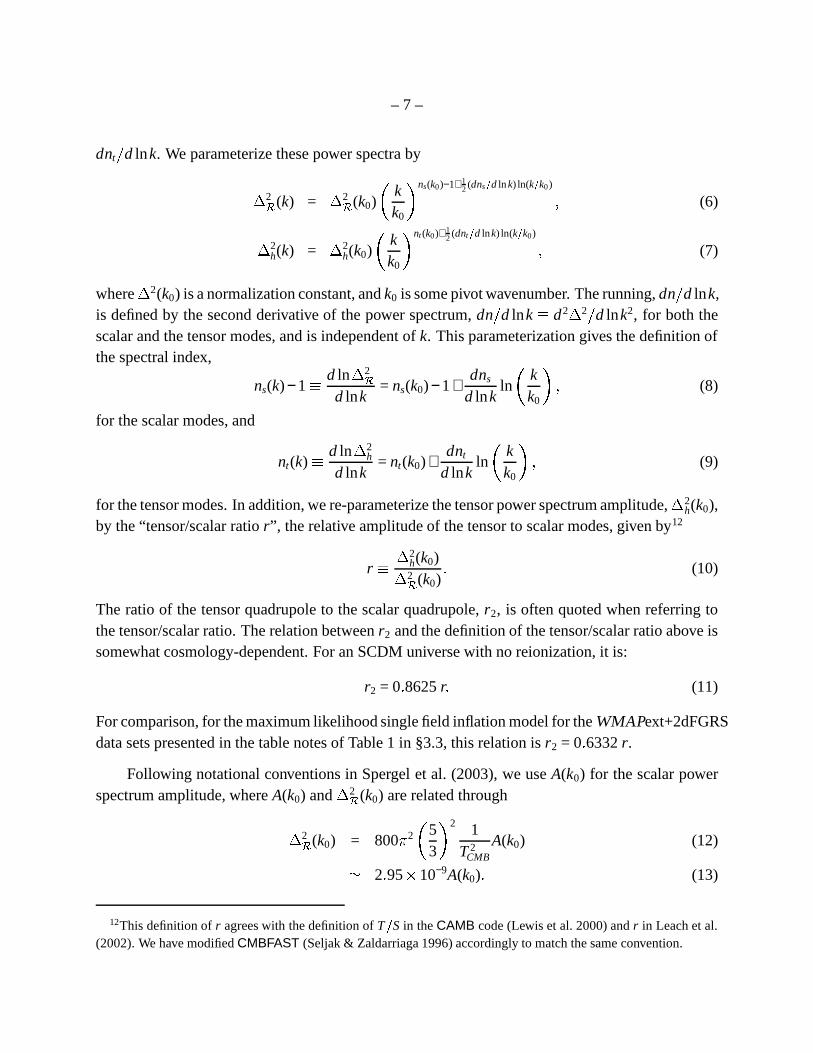
dnt � d lnk. We parameterize these power spectra by� 2� (k) =� 2� (k0) � k

k0 � ns(k0)−1+ 12 (dns � d ln k) ln(k � k0) � (6)� 2

h(k) =� 2

h(k0) � kk0 � nt (k0)+ 1

2 (dnt � d lnk) ln(k � k0) � (7)

where� 2(k0) is a normalization constant, and k0 is some pivot wavenumber. The running, dn � d lnk,

is defined by the second derivative of the power spectrum, dn � d lnk � d2 � 2 � d lnk2, for both thescalar and the tensor modes, and is independent of k. This parameterization gives the definition ofthe spectral index,

ns(k) − 1 � d ln� 2�

d lnk= ns(k0) − 1 +

dns

d lnkln � k

k0 � � (8)

for the scalar modes, and

nt(k) � d ln� 2

h

d lnk= nt(k0) +

dnt

d lnkln � k

k0 � � (9)

for the tensor modes. In addition, we re-parameterize the tensor power spectrum amplitude,� 2

h(k0),by the “tensor/scalar ratio r”, the relative amplitude of the tensor to scalar modes, given by12

r �� 2

h(k0)� 2� (k0)� (10)

The ratio of the tensor quadrupole to the scalar quadrupole, r2, is often quoted when referring tothe tensor/scalar ratio. The relation between r2 and the definition of the tensor/scalar ratio above issomewhat cosmology-dependent. For an SCDM universe with no reionization, it is:

r2 = 0 � 8625 r� (11)

For comparison, for the maximum likelihood single field inflation model for the WMAPext+2dFGRSdata sets presented in the table notes of Table 1 in §3.3, this relation is r2 = 0 � 6332 r.

Following notational conventions in Spergel et al. (2003), we use A(k0) for the scalar powerspectrum amplitude, where A(k0) and

� 2� (k0) are related through� 2� (k0) = 800 � 2 � 53 � 2 1

T 2CMB

A(k0) (12)� 2 � 95 � 10−9A(k0) � (13)

12This definition of r agrees with the definition of T � S in the CAMB code (Lewis et al. 2000) and r in Leach et al.(2002). We have modified CMBFAST (Seljak & Zaldarriaga 1996) accordingly to match the same convention.

– 8 –

Here, TCMB = 2 � 725 � 106 ( � K). This relation is derived in Verde et al. (2003). One can useequations (6), (8), and (9) to evaluate A, ns, and nt at a different wavenumber from k0, respectively.Hence,

A(k1) = A(k0) � k1

k0 � ns(k0)−1+ 12 (dns � d lnk) ln(k1 � k0)

� (14)

We have 6 observables (A, r, ns, nt , dns � d lnk, dnt � d lnk), each of which can be compared topredictions of an inflationary model.

The complementary approach (which we do not investigate in this work) is to parameterizethe primordial power spectrum in a model-independent way (see, for example, Wang et al. (1999)).These authors anticipated that WMAP has the potential ability to reveal deviations from scale-invariance when combined with large scale structure data. Mukherjee & Wang (2003a,b) extendthis approach and use it to put model-independent constraints on the primordial power spectrumusing the pre-WMAP CMB data.

3.2.2. Slow roll parameters

In the context of slow roll inflationary models, only three “slow-roll parameters”, plus theamplitude of the potential, determine the six observables (A, r, ns, nt , dns � d lnk, dnt � d lnk). Thus,one can use the relations among the observables to either reduce the number of parameters tofour, or cross-check if the slow roll inflation paradigm is consistent with the data. The slow-rollparameters are defined by (Liddle & Lyth 1992, 1993):

�V � M2

pl

2� V�

V � 2 � (15)�V � M2

pl� V� �

V � � (16)

�V � M4

pl� V�V� � �

V 2 � � (17)

where prime denotes derivatives with respect to the field�

. Here, �V quantifies “steepness” of the

slope of the potential which is positive-definite,�

V quantifies “curvature” of the potential, and�

V ,(which is not positive-definite, but is unfortunately often denoted

� 2 in the literature because it is asecond order parameter), quantifies the third derivative of the potential, or “jerk”. All parametersmust be smaller than one for inflation to occur. We denote these “potential slow roll” parameterswith a subscript V to distinguish them from the “Hubble slow roll” parameters of Appendix A.Gratton et al. (2003) discuss the equivalent set of parameters for the Ekpyrotic scenario.

– 9 –

Parameterization of slow roll models by �V ,�

V , and�

V avoids relying on specific models, andenables one to explore a large model space without assuming a specific model. Each inflationmodel predicts the slow-roll parameters, and hence the observables. A standard slow roll analysisgives observable quantities in terms of the slow roll parameters to first order as (see Liddle & Lyth(2000) for a review),� 2� =

V � M4pl

24 � 2 �V

� (18)

r = 16 �V � (19)

ns − 1 = −6 �V + 2

�V = −

3r8

+ 2�

V � (20)

nt = −2 �V = −

r8� (21)

dns

d lnk= 16 �

V

�V − 24 � 2

V − 2�

V = r�

V −332

r2 − 2�

V = −23�(ns − 1)2 − 4

� 2V � − 2

�V � (22)

dnt

d lnk= 4 �

V

�V − 8 � 2

V =r8

�(ns − 1) +

r8 � � (23)

The tensor tilt in inflation is always red, nt � 0. The equation nt = −r � 8 is known as the consis-tency relation for single-field inflation models (it weakens to an inequality for multi-field inflationmodels). We use the relation to reduce the number of parameters. While we have also carriedout the analysis including nt as a parameter, and verified that there is a parameter space satisfyingthe consistency relation, including nt obviously weakens the constraints on the other observables.Given that we find r is consistent with zero (§ 3.3), the running tensor index dnt � d lnk is poorlyconstrained with our data set; thus, we ignore it and constrain our models using the other fourobservables (A, r, ns, dns � d lnk) as free parameters.

3.3. Determining the power spectrum parameters

We use a Markov Chain Monte Carlo (MCMC) technique to explore the likelihood surface.Verde et al. (2003) describe our methodology. We use the WMAP TT (Hinshaw et al. 2003) andTE (Kogut et al. 2003) angular power spectra. To measure the shape of the spectrum (i.e., ns anddns � d lnk) accurately, we want to probe the primordial power spectrum over as wide a range ofscales as possible. Therefore, we also include the CBI (Pearson et al. 2002) and ACBAR (Kuoet al. 2002) CMB data, Lyman � forest data (Croft et al. 2002; Gnedin & Hamilton 2002), and the2dFGRS large-scale structure data (Percival et al. 2001) in our likelihood analysis. We refer to thecombined WMAP+CBI+ACBAR data as WMAPext.

In total, the single field inflation model is described by an 8-parameter model: 4 parametersfor characterizing a Friedmann-Robertson-Walker universe (baryonic density � bh2, matter density

– 10 –

� mh2, Hubble constant in units of 100 kms−1Mpc−1 h, optical depth � ), and 4 parameters for theprimordial power spectra (A, r, ns, dns � d lnk). When we add 2dFGRS data, we need two furtherlarge-scale structure parameters,

�and � p, to marginalize over the shape and the amplitude of

the 2dFGRS power spectrum (Verde et al. 2003). We run MCMC with these eight (WMAP onlymodel) or ten (WMAPext+2dFGRS, WMAPext+2dFGRS+Ly � models) parameters in order toget our constraints.

The priors on the model are: a flat universe, a cosmological constant equation of state for thedark energy, and a restriction of � � 0 � 3.

–11

–

Table 1. Parameters For Primordial Power Spectra: Single Field Inflation Model

Parameter WMAPa WMAPext+2dFGRSa WMAPext+2dFGRS+Lyman � a

ns(k0 = 0 � 002 Mpc−1) 1 � 20+0 � 12−0 � 11 1 � 18+0 � 12

−0 � 11 1 � 13

�

0 � 08r(k0 = 0 � 002 Mpc−1) � 1 � 28

�

0 � 81

�

0 � 47b � 1 � 14

�

0 � 53

�

0 � 37b � 0 � 90

�

0 � 43

�

0 � 29b

dns

�

d lnk −0 � 077+0 � 050−0 � 052 −0 � 075+0 � 044

−0 � 045 −0 � 055+0 � 028−0 � 029

A(k0 = 0 � 002 Mpc−1) 0 � 71+0 � 10−0 � 11 0 � 73

�

0 � 09 0 � 75+0 � 08−0 � 09

�

bh2 0 � 024

�

0 � 002 0 � 023

�

0 � 001 0 � 024�

0 � 001

�

mh2 0 � 127

�

0 � 017 0 � 134

�

0 � 006 0 � 134�

0 � 006h 0 � 78

�

0 � 07 0 � 75+0 � 03−0 � 04 0 � 75

�

0 � 03

� 0 � 22

�

0 � 06 0 � 20

�

0 � 06 0 � 18

�

0 � 06

�

8 0 � 82+0 � 13−0 � 12 0 � 85

�

0 � 05 0 � 85

�

0 � 05

aThe quoted values are the mean and the 68% probability level of the 1–d marginalized likelihood. Forboth WMAPext+2dFGRS and WMAPext+2dFGRS+Lyman � data sets, the 10–d maximum likelihoodpoint in the Markov Chain (1 � 5 106 steps) for this model is [

�

bh2 = 0 � 024,

�

mh2 = 0 � 132, h = 0 � 77,n(k0 � 002) = 1 � 15, r(k0 � 002) = 0 � 42, dns

�

d lnk = −0 � 052, A(k0 � 002) = 0 � 75, � = 0 � 21, �

8 = 0 � 87]. Here, k0 � 002 isk0 = 0 � 002 Mpc−1. The maximum likelihood model in the MCMC using WMAP data alone is [

�

bh2 =0 � 023,

�

mh2 = 0 � 122, h = 0 � 79, n(k0 � 002) = 1 � 27, r(k0 � 002) = 0 � 56, dns

�

d lnk = −0 � 10, A(k0 � 002) = 0 � 74,

� = 0 � 29]. Great care must be taken in interpreting this point. It is given here for completeness only,and we do not recommend it for use in any analysis. There is a long, flat degeneracy between n and

�, as described in §3 Spergel et al. (2003), and this point happened to lie at the very blue edge of thisdegeneracy right at the edge of our upper limit prior on �. This Markov chain had extra freedom becausewe are adding three parameters over the model discussed in Spergel et al. (2003), thereby introducingsignificant new degeneracies (see Figure 3).

bThe 95% upper limits for the tensor-scalar ratio are quoted for various priors in the following order:[no prior on dns

�

d lnk or ns] / [dns

�

d lnk= 0] / [ns

� 1]. The priors were applied to the output of theMCMC.

– 12 –

Table 1 shows results of our analysis for the WMAP, WMAPext+ 2dFGRS and WMAPext+2dFGRS + Lyman � data sets. We evaluate ns, A, and r in the fit at k0 = 0 � 002 Mpc−1. Thus, thistable and the figures to follow report the results for A and ns at k0 = 0 � 002 Mpc−1 . Note that Spergelet al. (2003) report these quantities evaluated at k0 = 0 � 05 Mpc−1 (using equations (14) and (8)).There are 3 � 2 e–folds between k0 = 0 � 002 Mpc−1 and k0 = 0 � 05 Mpc−1.

We did not find any tensor modes. Table 1 shows 95% upper limits for the tensor-scalar ratior at k = 0 � 002 Mpc−1, for various combinations of the data sets. As we will see later, there arestrong degeneracies present between the parameters ns, r and dns � d lnk. For example, one can addpower at low multipoles by increasing r and then remove it with a bluer ns while keeping the lowl amplitude constant. Thus, one can obtain stronger constraints on r by assuming different priorson ns and dns � d lnk. In the table, we list the 95% CL constraints on r that would be obtained if (1)there were no priors on ns or dns � d lnk, (2) if one only considers models with no running of thescalar spectral index, and (3) if only models with red spectral indices are considered (non-hybrid-inflation models predict red indices in general).

The no-prior r limit r � 0 � 9, along with the 2– � upper limit on the amplitude A(k = 0 � 002 Mpc−1) �0 � 75 + 0 � 08 � 2, implies that the energy scale of inflation V 1 � 4 � 3 � 3 � 1016 GeV at the 95% confi-dence level.

Note that in the case of the WMAP-only Markov chain, the degeneracy between ns, r anddns � d lnk is cut off by the prior � � 0 � 3 ( � is denegerate with ns). Thus, a better upper limit on �

will significantly tighten the constraints on this model from the WMAP data alone.

All cosmological parameters are consistent with the best-fit running model of Spergel et al.(2003), which was obtained for a � CDM model with no tensors and a running spectral index.Adding the extra parameter r does not improve the fit.

Our constraint on ns shows that the scalar power spectrum is nearly scale-invariant. Oneimplication of this result is that fluctuations were generated during accelerated expansion in nearlyde-Sitter space (Mukhanov & Chibisov 1981; Hawking 1982; Guth & Pi 1982; Starobinsky 1982;Bardeen et al. 1983; Mukhanov et al. 1992), where the equation of state of the scalar field is w � −1.Recently, Gratton et al. (2003) have shown that there is only one other possibility for robustlyobtaining adiabatic fluctuations with nearly scale-invariant spectra: w � 1. The Ekpyrotic/Cyclicscenarios correspond to this case. Note, however, that predictions for the primordial perturbationspectrum resulting from the Ekpyrotic scenario are controversial (see, for example, Tsujikawa et al.(2002)).

We find a marginal 2 � preference for a running spectral index in all three data sets; dns � d lnk =−0 � 055+0 � 028

−0 � 029 (WMAPext+2dFGRS+Lyman � data set). This same preference was seen in the anal-ysis without tensors carried out in Spergel et al. (2003).

– 13 –

Figure 2 shows our constraint on ns as a function of k for the WMAP, WMAPext+ 2dFGRSand WMAPext+ 2dFGRS + Lyman � data sets. At each wavenumber k, we use equation (8) toconvert ns(k0 = 0 � 002 Mpc−1) to ns(k) at each wavenumber. Then, we evaluate the mean (solidline), 68% interval (shaded area), and 95% interval (dashed lines) from the MCMCs. This showsa hint that the spectral index is running from blue (ns � 1) on large scales to red (ns � 1) on smallscales. In our MCMCs, for the WMAP data set alone, 91% of models explored by the chain havea scalar spectral index running from blue at k = 0 � 0007 Mpc−1 (l � 10) to red at k = 2 Mpc−1. Forthe WMAPext+2dFGRS data set, 95% of models go from a blue index at large scales to a redindex at small scales, and when Lyman � forest data is added, the fraction running from blue tored becomes 96%.

One-loop correction and renormalization usually predict running mass and/or running cou-pling constant, giving some dns � d lnk. Detection of it implies interesting quantum phenomenaduring inflation (see Lyth & Riotto (1999) for a review). For the running of the scalar spectralindex (equation 22),

dns

d lnk= −2

�V −

23�(ns − 1)2 − 4

� 2V � � (24)

Since the data requires ns � 1 (see Table 1), (ns − 1)2�

0 � 01. It is especially small when ns −1 � 2

�V , (see Case A and Case D in § 3.4.2). Therefore, if dns � d lnk is large enough to detect,

dns � d lnk � 10−2, then dns � d lnk must be dominated by 2�

V , a product of the first and the thirdderivatives of the potential (equation (17)). The hint of dns � d lnk in our data can be interpretedas

�V � − 1

2dns � d lnk = 0 � 028 � 0 � 015. However, obtaining the running from blue to red, which issuggested by the data, may require fine-tuned properties in the shape of the potential. More dataare required to determine whether the hints of a running index are real.

3.4. Single field models confront the data

3.4.1. Testing a specific inflation model:��� 4

As a prelude to showing constraints on broad classes of inflationary models, we first illustratethe power of the data using the example of the minimally-coupled V =

��� 4 � 4 model, which is oftenused as an introduction to inflationary models (Linde 1990). We show that this textbook exampleis unlikely.

The Friedmann and continuity equations for a homogeneous scalar field lead to the slow-rollparameters, which one can use in conjunction with the equations of § 3.2.2 in order to obtainpredictions for the observables. For the potential V (

�) =

� � 4 � 4, one obtains the potential slow roll

– 14 –

parameters as:

�V = 8

M2pl�2� �

V = 12M2

pl�2� �

V = 96M4

pl�4� (25)

The number of e-foldings remaining till the end of inflation is defined by

N = � tend

tHdt � 1

M2pl� ��

end

VV� d

�=

18

� � 2 −� 2

end

M2pl � � (26)

where �V (�

end) = 1 defines the end of inflation. Assuming�

end � �, taking the horizon exit scale

as� � � 8NMpl and N = 50, one obtains ns = 0 � 94 and r = 0 � 32 using equations (19) and (20). As

dns � d lnk is negligible for this model, we use dns � d lnk = 0.

We maximize the likelihood for this model by running a simulated annealing code. We fitto WMAPext+2dFGRS data, varying the following parameters: � bh2, � mh2, h, � , A13,

�, and � p,

while keeping ns, dns � d lnk, and r fixed at the��� 4 values. The maximum likelihood model ob-

tained has [ � bh2 = 0 � 022, � mh2 = 0 � 135, � = 0 � 07, A = 0 � 67, h = 0 � 69, � 8 = 0 � 76]. This best-fit modelis compared in Table 2 to the corresponding model with the full set of single field inflationary pa-rameters. The

��� 4 model is displaced from the maximum likelihood generic single field model by��� 2e f f = 16 [

��� 2e f f (WMAP) = 14,

��� 2e f f (CBI+ACBAR+2dFGRS) = 2], where

� 2e f f = −2ln � and� is the likelihood (see Verde et al. (2003)). Since the relative likelihood between the models is

exp(−8), and the number of degrees of freedom is approximately three,��� 4 is disfavored at more

than 3 � . The table shows that adding external data sets does not make a significant difference tothe

��� 2e f f between the models, and the constraint is primarily coming from WMAP data.

This result holds only for Einstein gravity. When a non-minimal coupling of the form� � 2R

(�

= 1 � 6 is the conformal coupling) is added to the Lagrangian, the coupling changes the dynamicsof�

. This model predicts only a tiny amount of tensor modes (Komatsu & Futamase 1999; Hwang& Noh 1998) in agreement with the data.

13While A is an inflationary parameter, it is directly related to the self-coupling � which we do not know; thus, wetreat it as a parameter.

– 15 –

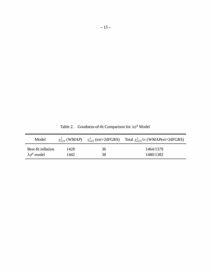
Table 2. Goodness-of-fit Comparison for��� 4 Model

Model� 2

e f f (WMAP)� 2

e f f (ext+2dFGRS) Total� 2

e f f ��� (WMAPext+2dFGRS)

Best-fit inflation 1428 36 1464/1379��� 4 model 1442 38 1480/1382

– 16 –

One can perform a similar analysis on any given inflationary model to see what constraints thedata put on it. Rather than attempt this Herculean task, in the following section we simply use ourconstraints on ns, dns � d lnk, and r and the predictions of various classes of single field inflationarymodels for these parameters in order to put broad constraints on them.

3.4.2. Testing a broad class of inflation models

Naively, the parameter space in observables spanned by the slow roll parameters appearsto be large. We shall show below that “viable” slow roll inflation models (i.e. those that cansustain inflation for a sufficient number of e-folds to solve cosmological problems) actually occupysignificantly smaller regions in the parameter space.

Hoffman & Turner (2001); Kinney (2002a); Easther & Kinney (2002); Hansen & Kunz (2002);Caprini et al. (2003) have investigated generic predictions of slow roll inflation models by using aset of inflationary flow equations (see Appendix A for a detailed description and definition of con-ventions). In particular Kinney (2002a) and Easther & Kinney (2002) use Monte Carlo simulationsto extend the slow roll approximations to fifth order. These authors find “attractors” correspondingto fixed points (where all derivatives of the flow parameters vanish); models cluster strongly nearthe power-law inflation predictions, r = 8(1 − ns) (see § 3.4.4), and on the zero tensor modes, r = 0.

Following the method of Kinney (2002a) and Easther & Kinney (2002), we compute a millionrealizations of the inflationary flow equations numerically, truncating the flow equation hierarchyat eighth order and evaluating the observables to second order in slow roll using equations (A15)–(A17). We marginalize over the ambiguity of converting between

�and k, introduced by the details

of reheating and the energy density during inflation by adopting the Monte Carlo approach of theabove authors. The observable quantities of a given realization of the flow equations are evaluatedat a specific value of e-folding, N. However, observable quantities are measured at a specific valueof k. Therefore, we need to relate N to k. This requires detailed modeling of reheating, whichcarries an inherent uncertainty. We attempt to marginalize over this by randomly drawing N valuesfrom a uniform distribution N = [40 � 70].

Figure 3 shows part of the parameter space of viable slow roll inflation models, with theWMAP 95% confidence region shown in blue. Each point on these panels is a different MonteCarlo realization of the flow equations, and corresponds to a viable slow roll model. Not all pointsthat are viable slow roll models correspond to specific physical models constructed in the literature.Most of the models cluster near the attractors, sparsely populating the rest of the large parameterspace allowed by the slow roll classification. It must be emphasized that these scatter plots shouldnot be interpreted in a statistical sense since we do not know how the initial conditions for the

– 17 –

universe are selected. Even if a given realization of the flow equations does not sit on the attractor,this does not mean that it is not favored. Each point on this plot carries equal weight, and eachis a viable model of inflation. Notice that the WMAP data do not lie particularly close to ther = 8(1 − ns) “attractor” solution, at the 2- � level, but is quite consistent with the r = 0 attractor.

One may categorize slow roll models into several classes depending upon where the predic-tions lie on the parameter space spanned by ns, dns � d lnk, and r (Dodelson et al. 1997; Kinney1998; Hannestad et al. 2001). Each class should correspond to specific physical models of infla-tion. Hereafter, we drop the subscript V unless there is an ambiguity — it should otherwise beimplicitly assumed that we are referring to the standard slow roll parameters. We categorize themodels on the basis of the curvature of the potential

�, as it is the only parameter that enters into

the relation between ns and r (equation (20)), and between ns and dns � d lnk + 2�

(equation (22)).Thus,

�is the most important parameter for classifying the observational predictions of the slow

roll models. The classes are defined by

(A) negative curvature models,� � 0,

(B) small positive (or zero) curvature models, 0� � �

2 � ,

(C) intermediate positive curvature models, 2 � � � �3 � , and

(D) large positive curvature models,� � 3 � .

Each class occupies a certain region in the parameter space. Using�

= (ns − 1) � � [2( � − 3)], where�= � � , one finds

(A) ns � 1, 0�

r � 83 (1 − ns), − 2

3(1 − ns)2 � dns � d lnk + 2� � 0,

(B) ns � 1, 83 (1 − ns)

�r

�8(1 − ns), − 2

3 (1 − ns)2 �dns � d lnk + 2

� �2(1 − ns)2,

(C) ns � 1, r � 8(1 − ns), dns � d lnk + 2� � 2(1 − ns)2, and

(D) ns � 1, r � 0, dns � d lnk + 2� � 0.

To first order in slow roll, the subspace (ns, r) is uniquely divided into the four classes, and thewhole space spanned by these parameters is defined by this classification. The division of theother subspace (ns, dns � lnk) is less unique, and dns � d lnk � −2

�− 2

3 (1 − ns)2 is not covered bythis classification. To higher order in slow roll, these boundaries only hold approximately - forinstance, Case C can have a slightly blue scalar index, and Case D can have a slightly red one.

– 18 –

We summarize basic predictions of the above model classes to first order in slow roll usingthe relation between r and ns (equation (20)) rewritten as

r =83

(1 − ns) +163

� � (27)

This implies:

(A) negative curvature models predict� � 0 and 1 − ns � 0; the second term nearly cancels the

first to give r too small to detect,

(B) small positive curvature models predict 1 − ns � 0 and� � 0; a large r is produced,

(C) intermediate positive curvature models predict 1 − ns � 0 and� � 0; a large r is produced,

and

(D) large positive curvature models predict 1 − ns � 0 and� � 0; the first term nearly cancels the

second to give r too small to detect.

The cancellation of the terms in Case A and Case D implies ns −1 � 2�: the steepness of the poten-

tial in Case A and Case D is insignificant compared to the curvature, � � � � �. On the other hand, in

Case B and Case C the steepness is larger than or comparable to the curvature, by definition; thus,non-detection of r can exclude many models in Case B and Case C. As we have shown in § 3.4.1,a minimally-coupled

��� 4 model, which falls into Case B, is excluded at high significance, largelybecause of our non-detection of r (see also § 3.4.4).

For an overview, Figure 4 shows the Monte Carlo flow equation realizations correspondingto the model classes A–D above on the (ns, r), (ns, dns � d lnk), and (r, dns � d lnk) planes, for theWMAP, WMAPext+2dFGRS and WMAPext+2dFGRS+Lyman � data sets.

In Table 3, we show the ranges taken by the observables ns, r and dns � d lnk in the MonteCarlo realizations that remain after throwing out all the points which are outside at least one ofthe joint-95% confidence levels. These points have been separated into the model classes A–D viatheir

�V . These constraints were calculated as follows. First, we find the Monte Carlo realizations

of the flow equations from each model class that fall inside all the joint-95% confidence levels fora given data set, separately for the WMAP, WMAPext+2dFGRS and WMAPext+2dFGRS+Lyman

� data sets (i.e. the models shown on Figure 4). Then we find for each model class the maximumand minimum values predicted for each of the observables within these subsets. These constraintsmean that only those models (within each class) predicting values for the observables that lieoutside these limits are excluded by these data sets at 95% CL. Note that the best-fit model withinthis parameter space has a

� 2e f f ��� = 1464 � 1379. Here, recall again that the observables were

– 19 –

evaluated to second order in slow roll in these calculations. This is the reason that the Class Crange in ns goes slightly blue and the Class D range in ns goes slightly red; the divisions of the

�V

classification are only exact to first order in slow roll.

In the following subsections we will discuss in more detail the constraints on specific phys-ical models that fall into the classes A–D. For a given class, we will plot only the flow equationrealizations falling into that category that are consistent with the 95% confidence regions of all theplanes (ns, r), (ns, dns � d lnk) and (r, dns � d lnk).

–20

–

Table 3. Properties of Inflationary Models Present Within the Joint-95% Confidence Regiona

Model WMAP WMAPext+2dFGRS WMAPext+2dFGRS+Lyman �A (4 10−6)b �

r

�

0 � 14 (2 10−6)b �

r

�

0 � 19 (4 10−6)b �

r

�

0 � 160 � 94

�

ns

�

1 � 00 0 � 93

�

ns

�

1 � 00 0 � 94

�

ns

�

1 � 00−0 � 02

�

dns

�

d lnk

�

0 � 02 −0 � 04

�

dns

�

d lnk

�

0 � 02 −0 � 02

�

dns

�

d lnk�

0 � 004B (7 10−3)b �

r

�

0 � 35 (7 10−3)b �

r

�

0 � 32 (7 10−3)b �

r

�

0 � 260 � 94

�

ns

�

1 � 01 0 � 93

�

ns

�

1 � 01 0 � 94

�

ns

�

1 � 01−0 � 02

�

dns

�

d lnk

�

0 � 02 −0 � 04

�

dns

�

d lnk

�

0 � 02 −0 � 02

�

dns�

d lnk

�

0 � 01C (0 � 003)b �

r

�

0 � 59 (0 � 003)b �

r

�

0 � 52 (0 � 03)b �

r�

0 � 460 � 95

�

ns

�

1 � 02 0 � 96

�

ns

�

1 � 02 0 � 97�

ns

�

1 � 02−0 � 04

�

dns

�

d lnk

�

0 � 01 −0 � 04

�

dns

�

d lnk

�

0 � 01 −0 � 04

�

dns

�

d lnk

�

0 � 001D 0 � 0

�

r

�

1 � 10 0 � 0

�

r

�

0 � 89 (8 10−5)b �

r

�

0 � 890 � 99

�

ns

�

1 � 28 1 � 00

�

ns

�

1 � 28 1 � 00

�

ns

�

1 � 28−0 � 09

�

dns

�

d lnk

�

0 � 03 −0 � 09

�

dns

�

d lnk�

0 � 01 −0 � 09

�

dns

�

d lnk

� −0 � 001

aThe ranges taken by the predicted observables of slow roll models (to second order in slow roll)within the joint 95% CLs from the specified data sets. The model classes are: Case A ( � � 0), Case B(0

� � �

2 �), Case C (2 � � � �

3 �), Case D ( � � 3 �).

bThe lower value of r does not represent a detection, but rather the minimal level of tensors predictedby any point in the Monte Carlo that falls within in this class and is consistent with the data. Weinclude the lower limit to help set goals for future CMB polarization missions.

– 21 –

Note that very few models predict a “bad power law”, or�dns � d lnk

� � 0 � 05.

3.4.3. Case A: negative curvature models� � 0

The top row of Figure 5 shows the Monte Carlo points belonging to Case A which are con-sistent with all the joint-95% confidence regions of the observables shown in the figure, for theWMAPext+2dFGRS+Lyman � data set.

The negative�

models often arise from a potential of spontaneous symmetry breaking (e.g.,new inflation - Albrecht & Steinhardt (1982); Linde (1982)).

We consider negative-curvature potentials in the form of V = � 4[1 − (� � � )p] where p � 2.

We require� � � for the form of the potential to be valid, and � determines the energy scale of

inflation, or the energy stored in a false vacuum. One finds that this model always gives a red tiltns � 1 to first order in slow roll, as ns − 1 = −6 � − 2

� � � � 0.

For p = 2, the number of e-folds at�

before the end of inflation is given by N � ( � 2 � 2M2pl) ln( � � � ),

where we have approximated�

end � � . By using the same approximation, one finds ns − 1 �−4(Mpl � � )2, and r � 32(

� 2M2pl � � 4) � 8(1 − ns)e−N(1−ns ). In this class of models, ns cannot be very

close to 1 without � becoming larger than mpl. For example, ns = 0 � 96 implies � � 10Mpl � 2mpl.For this class of models, r has a peak value of r � 0 � 06 at ns = 0 � 98 (assuming N = 50). Even thispeak value is too small for WMAP to detect. We see from Table 3 that this model is consistentwith the current data, but requires � � mpl to be valid.

For p � 3, ns − 1 � −(2 � N)(p − 1) � (p − 2) or 0 � 92�

ns � 0 � 96 for N = 50 regardless of a valueof � , and r � 4p2(Mpl � � )2(

� � � )2(p−1) is negligible as� � � . These models lie in the joint 2– �

contour.

The negative�

model also arises from the potential in the form of V = � 4[1 + � ln(� � � )], a

one-loop correction in a spontaneously broken supersymmetric theory (Dvali et al. 1994). Herethe coupling constant � should be smaller than of order 1. In this model

�rolls down towards the

origin. One finds ns − 1 = −(1 + 32 � ) � N which implies 0 � 95 � ns � 0 � 98 for 1 � � � 0 (this formula

is not valid when � = 0 or�

= � ). Since r = 8 � � N = 8 � (1+ 32 � )−1(1−ns) = 0 � 016( � � 0 � 1), the tensor

mode is too small for WMAP to detect, unless the coupling � takes its maximal value, � � 1. Thistype of model is consistent with the data.

– 22 –

3.4.4. Case B: small positive curvature models 0� � �

2 �

The second row of Figure 5 shows the Monte Carlo points belonging to Case B which areconsistent with all the joint-95% confidence regions of the observables shown in the figure.

The “small” positive�

models correspond to monomial potentials for 0 � � � 2 � and expo-nential potentials for

�= 2 � . The monomial potentials take the form of V = � 4(

� � � )p where p � 2,and the exponential potentials V = � 4 exp(

� � � ). The zero�

model is V = � 4(� � � ). To first order in

slow roll, the scalar spectral index is always red, as ns − 1 = −6 � + 2� � −4 � � 0. The zero

�model

marks a border between the negative�

models and the positive�

models, giving r = 83 (1 − ns).

The monomial potentials often appear in chaotic inflation models (Linde 1983), which requirethat

�be initially displaced from the origin by a large amount, � mpl, in order to avoid fine-tuned

initial values for�

. The monomial potentials can have a period of inflation at���

mpl, and inflationends when

�rolls down to near the origin. For p = 2, inflation is driven by the mass term, which

gives�

= 2 � NMpl, ns = 1 − 2 � N = 0 � 96, r = 8 � N = 4(1 − ns) = 0 � 16, and dns � d lnk = −2 � N2 = −(1 −ns)2 � 2 = −0 � 8 � 10−3. For p = 4, inflation is driven by the self-coupling, which gives

�= 2 � 2NMpl,

ns = 1−3 � N = 0 � 94, r = 16 � N = 163 (1−ns) = 0 � 32, and dns � d lnk = −3 � N2 = −(1−ns)2 � 3 = −1 � 2 � 10−3.

The most striking feature of the small positive�

models is that the gravitational wave amplitudecan be large, r � 0 � 16. Our data suggest that, for monomial potentials to lie within the joint95% contour, r � 0 � 26 (Table 3). A

��� 4 model is excluded at � 3– � (§ 3.4.1), and any monomialpotentials with p � 4 are also excluded at high signifcance. Models with p = 2 (mass term inflation)are consistent with the data.

The exponential potentials appear in the Brans–Dicke theory of gravity (Brans & Dicke 1961;Dicke 1962) conformally transformed to the Einstein frame (the extended inflation models) (La &Steinhardt 1989). One finds ns = 1−( � � Mpl)2, r = 8(1−ns), and dns � d lnk = 0. Thus, the exponentialpotentials predict an exact power-law spectrum and significant gravitational waves for significantlytilted spectra. Since � = NM2

pl � (�

−�

end), ns = 1− [NMpl � (�

−�

end)]2. The 95% range for ns in Table3 implies that

�−�

end � 4NMpl � 200Mpl � 40mpl.

The exponential potentials mark a border between the small positive�

models and the positiveintermediate

�models described below.

3.4.5. Case D: large positive curvature models� � 3 �

Before describing Case C, it is useful to describe Case D first. The fourth row of Figure 5shows the Monte Carlo points belonging to Case D which are consistent with all the joint-95%confidence regions of the observables shown in the figure.

– 23 –

The “large” positive curvature models correspond to hybrid inflation models (Linde 1994),which have recently attracted much attention as an R-invariant supersymmetric theory naturallyrealizes hybrid inflation (Copeland et al. 1994; Dvali et al. 1994). While it is pointed out thatsupergravity effects add too large an effective mass to the inflaton field to maintain inflation, theminimal Kähler supergravity does not have such a large mass problem (Copeland et al. 1994; Linde& Riotto 1997). The distinctive feature of this class of models with

� � 3 � is that the spectrum hasa blue tilt, ns − 1 = −6 � + 2

� � 0, to first order in slow roll.

A typical potential is a monomial potential plus a constant term, V = � 4[1 + (� � � )p], which

enables inflation to occur for a small value of�

,� � mpl. At first sight, inflation never ends for this

potential, as the constant term sustains the exponential expansion forever. Hybrid inflation modelspostulate a second field � which couples to

�. When

�rolls slowly on the potential, � stays at the

origin and has no effect on the dynamics. For a small value of�

inflation is dominated by a falsevacuum term, V (

� � � = 0) � � 4. When�

rolls down to some critical value, � starts moving towarda true vacuum state, V (

� � � ) = 0, and inflation ends. A numerical calculation (Linde 1994) suggeststhat the potential is described by

�only until

�reaches a critical value. When

�reaches the critical

value, inflation suddenly ends and � need not be considered. Thus, we include the hybrid modelsin our discussion of single-field models.

For p = 2, one finds that N � 12 ( � � Mpl)2 ln(

� � � end) � 50, which, in turn, implies � � 10Mpl �2mpl for ln(

� � � end) � 1. The spectral slope is estimated as ns � 1 + 4(Mpl � � )2 � 1 � 04, and thetensor/scalar ratio, r � 32(

� � � )2(Mpl � � )2 = 8(� � � )2(ns −1), is negligible as inflation occurs at

� �� . The running is also negligible, as dns � d lnk � 64(� � � )2(Mpl � � )4 = 4(

� � � )2(ns − 1)2 � 10−2.This type of model lies within the joint 95% contours.

One-loop correction in a softly broken supersymmetric theory induces a logarithmically run-ning mass, V = � 4 � 1 + (

� � � )2 � 1 + � ln(� � Q) ��� , where � is a coupling constant and Q is a renor-

malization point. Since ns is practically determined by V� �, this potential gives rise to a logarithmic

running of ns (Lyth & Riotto 1999). These models would lie in the region occupied by the MonteCarlo points that have a large, negative dns � d lnk. This type of model is consistent with the data.

3.4.6. Case C: intermediate positive curvature models 2 � � � �3 �

The third row of Figure 5 shows the Monte Carlo points belonging to Case C which areconsistent with all the joint-95% confidence regions of the observables shown in the figure.

The “intermediate” positive curvature models are defined, to first order in slow roll, as havinga red tilt, ns − 1 = −6 � + 2

� � 0, or the exactly scale-invariant spectrum, ns − 1 = 0, while not beingdescribed by monomial or exponential potentials. These conditions lead to a parameter space

– 24 –

where 2 � � � �3 � . Here we discuss only examples of physical models that do not solely live in

Case C, but briefly pass through it as they transition from Case D to Case B or Case A.

The transition from Case D to Case B may correspond to a special case of hybrid inflationmodels described in the previous subsection (Case D), V = � 4[1 + (

� � � )p]. When� � � , the

potential becomes Case B potential, V � � 4(� � � )p, and the spectrum is red, ns � 1. When

� � � ,the potential drives hybrid inflation, and the spectrum is blue, ns � 1. On the other hand, when�

� � , the potential takes a parameter space somewhere between Case B and Case D, whichcorresponds to Case C. One may argue that this model requires fine-tuned properties in that we justtransition from one regime to the other. However, the Case C regime has an interesting property:the spectral index ns runs from red on large scales to blue on small scales, as

�undergoes the

transition from Case B to Case D. This example has the wrong sign for the running of the indexcompared to the data at the � 2- � level.

Linde & Riotto (1997) is one example of a transition from Case D to Case A. They considera supergravity-motivated hybrid potential with a one-loop correction, which can be approximatedduring inflation as

V � � 4 � 1 + � ln(� � Q) +

�(� � � )4 � � (28)

Suppose that the one-loop correction is negligible in some early time, i.e.,� � Q. The spectrum

is blue. (The third term is practically unimportant, as inflation is driven by the first term at thisstage.) If the loop correction becomes important after several e-folds, then ns changes from blue tored, as the loop correction gives a red tilt as we saw in § 3.4.3. This example is consistent with thedata. The transition (from Case D to Case A) is possible only when � and Q conspire to balancethe first term and the second term right at the scale accessible to our observations.

4. MULTIPLE FIELD INFLATION MODELS

4.1. Framework

In general, a candidate fundamental theory of particle physics such as a supersymmetric the-ory requires not only one, but many other scalar fields. It is thus naturally expected that duringinflation there may exist more than one scalar field that contributes to the dynamics of inflation.

In most single-field inflation models, the fluctuations produced have an almost scale-invariant,Gaussian, purely adiabatic power spectrum whose amplitude is characterized by the comovingcurvature perturbation,

�, which remains constant on superhorizon scales. They also predict tensor

perturbations with the consistency condition in equation (21).

With the addition of multiple fields, the space of possible predictions widens considerably.

– 25 –

The most distinctive feature is the generation of entropy, or isocurvature, perturbations betweenone field and the other. The entropy perturbation,

��, can violate the conservation of

�on super-

horizon scales, providing a source for the late-time evolution of�

which weakens the single fieldconsistency condition into an upper bound on the tensor/scalar ratio (Polarski & Starobinsky 1995;Sasaki & Stewart 1996; Garcia-Bellido & Wands 1996). Limits on the possible level of the entropyperturbation thus discriminate between the multiple field models and the single field models. Inthis section, we consider the minimal extension to single-field inflation – a model consisting of twominimally-coupled scalar fields.

4.2. Correlated Adiabatic/Isocurvature Fluctuations from Double-Field Inflation

The WMAP data confirm that pure isocurvature fluctuations do not dominate the observedCMB anisotropy. They predict large-scale temperature anisotropies that are too large with respectto the measured density fluctuations, and have the wrong peak/trough positions in the temperatureand polarization power spectra (Hu & White 1996; Page et al. 2003). The WMAP observationslimit but do not preclude the possibility of correlated mixtures of isocurvature and adiabatic pertur-bations, which is a generic prediction of two-field inflation models. Both isocurvature and adiabaticperturbations receive significant contributions from at least one of the scalar fields to produce thecorrelation (Langlois 1999; Pierpaoli et al. 1999; Langlois & Riazuelo 2000; Gordon et al. 2001;Bartolo et al. 2001, 2002; Amendola et al. 2002; Wands et al. 2002). We focus on these mixedmodels in this section.

Let�

rad and��rad be the curvature and entropy perturbations deep in the radiation era, respec-

tively. At large scales, the temperature anisotropy is given by (Langlois 1999):�T

T=

15

�rad − 2

��rad � (29)

in addition to the integrated Sachs–Wolfe effect. The entropy perturbation,��rad ����� cdm � � cdm −

(3 � 4) ����� � ��� , remains constant on large scales until re-entry into the horizon. If�

rad and��rad have

the same sign (correlated), then the large scale temperature anisotropy is reduced. If they haveopposite signs (anti-correlated), then the temperature anisotropy is increased. Spergel et al. (2003)find that there is an apparent lack of power at the very largest scales in the WMAP data; thus, oneof the motivations of this study is to see whether a correlated

��rad can provide a better fit to the

WMAP low-l data than a purely adiabatic model.

The evolution of the curvature/entropy perturbations from horizon-crossing to the radiation-

– 26 –

dominated era can be parameterized by a transfer matrix (Amendola et al. 2002),� �rad��rad � = � 1 TRS

0 TSS �� ����� � � k=aH

� (30)

Here, TRR = 1 and TSR = 0 because of the physical requirement that�

is conserved for purelyadiabatic perturbations, and that

�cannot source

��. All the quantities in equation (30) are weakly

scale-dependent, and may be parameterized by power-laws. Hence, we write this equation as�rad = Ark

n1�

ar + Askn3�

as � (31)��rad = Bkn2

�as � (32)

where�

ar and�

as are independent Gaussian random variables with unit variance,� �ar�

as � = � rs. Thecross-correlation spectrum is given by

� 2RS(k) � (k3 � 2 � 2)

� �rad

��rad � = AsBkn2+n3 . One may define

the correlation coefficient using an angle�

as

cos� �

� �rad

��rad �� �

2rad � 1 � 2 �

�� 2rad � 1 � 2

=sign(B)Askn3�A2

r k2n1 + A2s k2n3

� (33)

where −1�

cos� �

1. Thus, in general, six parameters (Ar, As, cos�

, n1, n2, n3) are needed tocharacterize the double-inflation model with correlated adiabatic/isocurvature perturbations, whilecos

�is scale-dependent. In order to simplify our analysis, we neglect the scale-dependence of

cos�

; thus, n1 = n3 �= n2 and cos�

= sign(B)As � A. The power spectra are written as� 2� (k) �

(k3 � 2 � 2)� �

2rad � = (A2

r + A2s )k2n1 � A2knad−1, and

� 2� (k) � (k3 � 2 � 2)� �� 2

rad � = B2k2n2 � A2 f 2isokniso−1. We

have defined nad − 1 � 2n1 and niso − 1 � 2n2 to coincide with the standard notation for the scalarspectral index. The “isocurvature fraction” defined by fiso � B � A determines the relative amplitudeof

��to

�. The cross-correlation spectrum is then written as

� 2RS(k) = cos

� � � 2� (k)� 2� (k) =

A2 fiso cos�

k(nad+niso) � 2−1.

The temperature and polarization anisotropies are given by these power spectra:

Cadl � A2 � dk

k� k

k0 � nad−1 �gad

l (k) � 2 � (34)

Cisol � A2 f 2

iso � dkk� k

k0 � niso−1 �giso

l (k) � 2 � (35)

Ccorrl � A2 fiso cos

� � dkk� k

k0 � (nad+niso) � 2−1 �gad

l (k)gisol (k) � � (36)

and the total anisotropy is Ctotl = Cad

l + Cisol + 2Ccorr

l . Here, gl(k) is the radiation transfer func-tion appropriate to adiabatic or isocurvature perturbations of either temperature or polarization

– 27 –

anisotropies. Note that the quantities nad , niso, and fiso are defined at a specific wavenumber k0,which we take to be k0 = 0 � 05 Mpc−1 in the MCMC. To translate the constraint on fiso to any otherwavenumber, one uses

fiso(k1) = fiso(k0) � k1

k0 � (niso−nad ) � 2� (37)

We can restrict fiso � 0 without loss of generality. Since we can remove A by normalizing to theoverall amplitude of fluctuations in the WMAP data, we are left with 4 parameters, nad , niso, fiso,and cos

�. We neglect the contribution of tensor modes, as the addition of tensors goes in the

opposite direction in terms of explaining the low amplitude of the low-l TT power spectrum. Wealso neglect the scale-dependence of nad and niso, as they are not well constrained by our data sets.

We fit to the WMAPext+2dFGRS and WMAPext+2dFGRS+Lyman � data sets with the 11parameter model ( � bh2, � mh2, h, � , nad , niso, fiso, cos

�, A,

�, � p). The results of the fit for

the double inflation model parameters are shown in Table 4. Figure 6 shows the cumulativedistribution of fiso. The best-fit non-primordial cosmological parameter constraints are very similarto the single field case.

– 28 –

Table 4. Cosmological Parameters: Adiabatic + Isocurvature Model

Parameter WMAPext+2dFGRS WMAPext+2dFGRS+Lyman �

fiso(k0 = 0 � 05 Mpc−1) � 0 � 32a � 0 � 33a

nad 0 � 97 � 0 � 03 0 � 95 � 0 � 03niso 1 � 26+0 � 51

−0 � 57 1 � 29+0 � 50−0 � 56

cos�

−0 � 76+0 � 18−0 � 14 −0 � 76+0 � 18

−0 � 16

A(k0 = 0 � 05 Mpc−1) 0 � 82 � 0 � 10 0 � 78 � 0 � 08� bh2 0 � 023 � 0 � 001 0 � 023 � 0 � 001� mh2 0 � 133 � 0 � 007 0 � 131 � 0 � 006h 0 � 072 � 0 � 04 0 � 072 � 0 � 04� 0 � 16 � 0 � 06 0 � 14 � 0 � 06� 8 0 � 84 � 0 � 06 0 � 81 � 0 � 04

aThe constraint on the isocurvature fraction, fiso, is a 95% upper limit.

– 29 –

While the fit tries to reduce the large-scale anisotropy with an admixture of correlated isocur-vature modes as expected (note that cos

� � 0 corresponds to�

rad and��rad having the same sign,

from the definition of initial conditions in the CMBFAST code), this only leads to a small reduc-tion in amplitude at the quadrupole. Table 5 compares the goodness-of-fit for this model along withthe maximum likelihood models for the � CDM and single field inflation cases. Because

� 2e f f ���

is not improved by the addition of three new parameters and considerable physical complexity,we conclude that the data do not require this model. This implies that the initial conditions areconsistent with being fully adiabatic.

– 30 –

Table 5. Goodness-of-Fit Comparison for Adiabatic/Isocurvature Model

Model� 2

e f f ��� a

� CDM 1468/1381Single field inflation 1464/1379Adiabatic/Isocurvature 1468/1378

aThese� 2

e f f values are for theWMAPext+2dFGRS data set. Herewe do not give

� 2e f f for the Lyman

� data, as the covariance between thedata points is not known (Verde et al.2003).

– 31 –

5. SMOOTHNESS OF THE INFLATON POTENTIAL

Spergel et al. (2003) point out that there are several sharp features in the WMAP TT angularpower spectrum that contribute to the reduced-

� 2e f f for the best-fit model being � 1 � 09. The large� 2

e f f may result from neglecting 0.5–1% contributions to the WMAP TT power spectrum covari-ance matrix; for example, gravitational lensing of the CMB, beam asymmetry, and non-Gaussianityin noise maps. When included, these effects will likely improve the reduced-

� 2e f f of the best-fit

� CDM model. At the moment we cannot attach any astrophysical reality to these features. Similarfeatures appear in Monte Carlo simulations.

While we do not claim these glitches are cosmologically significant, it is intriguing to considerwhat they might imply if they turn out to be significant after further scrutiny.

In this section we investigate whether the reduced-� 2

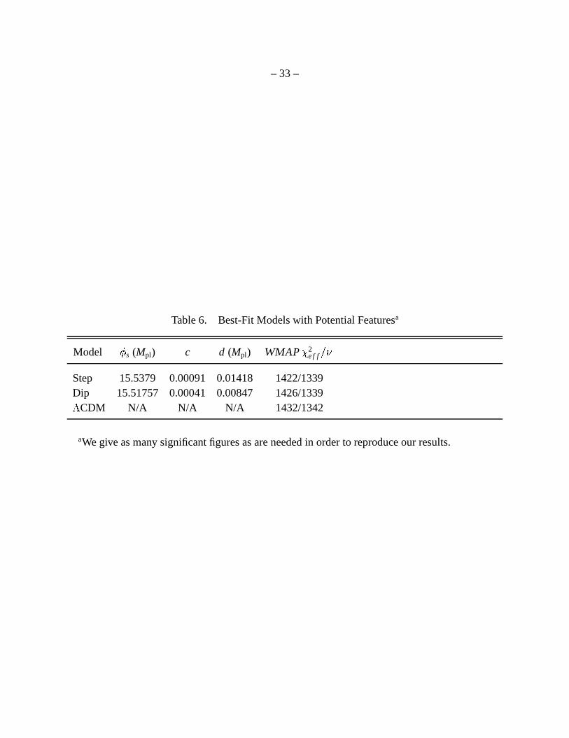
e f f is improved by trying to fit one ormore of these “glitches” with a feature in the inflationary potential. Adams et al. (1997) showthat a class of models derived from supergravity theories naturally gives rise to inflaton potentialswith a large number of sudden downward steps. Each step corresponds to a symmetry-breakingphase transition in a field coupled to the inflaton, since the mass changes suddenly when eachtransition occurs. If inflation occurred in the manner suggested by these authors, a spectral featureis expected every 10-15 e-folds. Therefore, one of these features may be visible in the CMB orlarge-scale structure spectra.

We use the formalism adopted by Adams et al. (2001), and model the step by the potential

Vstep(�

) =12

m2 � 2 � 1 + c tanh � � −�

s

d ��� � (38)

where�

is the inflaton field, and the potential has a step starting at�

s with amplitude and gradientdetermined by c and d respectively. In physically realistic models, the presence of the step doesnot interrupt inflation, but affects density perturbations by introducing scale-dependent oscillations.Adams et al. (2001) describe the phenomenology of these models: the sharper the step, the largerthe amplitude and longevity of the “ringing.” For our calculations of the power spectrum in thesemodels, we numerically integrate the Klein–Gordon equation using the prescription of Adams et al.(2001).

We also phenomenologically model a dip in the inflaton potential using a toy model of aGaussian dip centered at

�s with height c and width d:

Vdip(�

) =12

m2 � 2 � 1 − c exp � ( � −�

s)2

2d2 � � � (39)

We fix the non-primordial cosmological parameters at the maximum likelihood values forthe � CDM model fitted to the WMAPext data, [ � bh2 = 0 � 022, � mh2 = 0 � 13, � = 0 � 11, A = 0 � 74,

– 32 –

h = 0 � 72]. We then run simulated annealing codes for only the three parameters:�

s, c, and d,for each potential, fitting to the WMAP TT and TE data only. For this section, since this modelpredicts sharp features in the angular power spectrum, we had to modify the standard CMBFASTsplining resolution, splining at

�l = 1 for 2

�l � 50 and

�l = 5 for l � 50.

The best-fit parameters found for each potential are given in Table 6, along with the� 2

e f f forthe WMAP TT and TE data. Figure 7 shows these models plotted along with the WMAP TTdata. The best-fit models predict features in the TE spectrum at specific multipoles, which are wellbelow detection, given the current uncertainties. The step model differs from the � CDM model by��� 2

e f f = 10, the dip model by��� 2

e f f = 6. We are not claiming that these are the best possible modelsin this parameter space, only that these are the best-fit models found in 8 simulated annealing runs.Note that the models with features were not allowed the freedom to improve the fit by adjustingthe cosmological parameters.

– 33 –

Table 6. Best-Fit Models with Potential Featuresa

Model�

s (Mpl) c d (Mpl) WMAP� 2

e f f ���Step 15.5379 0.00091 0.01418 1422/1339Dip 15.51757 0.00041 0.00847 1426/1339

� CDM N/A N/A N/A 1432/1342

aWe give as many significant figures as are needed in order to reproduce our results.

– 34 –

A very small fractional change in the inflaton potential amplitude, c � 0 � 1%, is sufficientto cause sharp features in the angular power spectrum. Models with much larger c would havedramatic effects that are not seen in the WMAP angular power spectrum.

These models also predict sharp features in the large-scale structure power spectrum. Figure 8shows the matter power spectra for the best-fit step/dip models. Forthcoming large-scale structuresurveys may look for the presence of such features, and test the viability of these models.

6. CONCLUSIONS

WMAP has made six key observations that are of importance in constraining inflationarymodels.

(a) The universe is consistent with being flat (Spergel et al. 2003).

(b) The primordial fluctuations are described by random Gaussian fields (Komatsu et al. 2003).

(c) We have shown that the WMAP detection of an anti-correlation between CMB temperatureand polarization fluctuations at � � 2 � is a distinctive signature of adiabatic fluctuations onsuperhorizon scales at the epoch of decoupling. This detection agrees with a fundamentalprediction of the inflationary paradigm.

(d) In combination with complementary CMB data (the CBI and the ACBAR data), the 2dF-GRS large-scale structure data, and Lyman � forest data, WMAP data constrain the pri-mordial scalar and tensor power spectra predicted by single-field inflationary models. Forthe scalar modes, the mean and the 68% error level of the 1–d marginalized likelihood forthe power spectrum slope and the running of the spectral index are, respectively, ns(k0 =0 � 002 Mpc−1) = 1 � 13 � 0 � 08 and dns � d lnk = −0 � 055+0 � 028

−0 � 029. This value is in agreement withdns � d lnk = −0 � 031+0 � 016

−0 � 018 of Spergel et al. (2003), which was obtained for a � CDM modelwith no tensors and a running spectral index. The data suggest at the 2- � level, but do notrequire that, the scalar spectral index runs from ns � 1 on large scales to ns � 1 on smallscales. If true, the third derivative of the inflaton potential would be important in describingits dynamics.

(e) The WMAPext+2dFGRS constraints on ns, dns � d lnk, and r put limits on single-field in-flationary models that give rise to a large tensor contribution and a red (ns � 1) tilt. Aminimally-coupled

��� 4 model lies more than 3- � away from the maximum likelihood point.The contribution to the

� � 2 between the two points from WMAP alone is 14.

– 35 –

(f) We test two-field inflationary models with an admixture of adiabatic and CDM isocurvaturecomponents. The data do not justify adding the additional parameters needed for this model,and the initial conditions are consistent with being purely adiabatic.

WMAP both confirms the basic tenets of the inflationary paradigm and begins to quantita-tively test inflationary models. However, we cannot yet distinguish between broad classes of infla-tionary theories which have different physical motivations. In order to go beyond model buildingand learn something about the physics of the early universe, it is important to be able to make suchdistinctions at high significance. To accomplish this, one requirement is a better measurement ofthe fluctuations at high l, and a better measurement of � , in order to break the degeneracy betweenns and � .

We note that an exact scale-invariant spectrum (ns = 1 and dns � d lnk = 0) is not yet excluded atmore than 2 � level. Excluding this point would have profound implications in support of inflation,as physical single field inflationary models predict non-zero deviation from exact scale-invariance.

We conclude by showing the tensor temperature and polarization power spectra for the maxi-mum likelihood single-field inflation model for the WMAPext+2dFGRS+Lyman � data set, whichhas tensor/scalar ratio r = 0 � 42 (Figure 9). The detection and measurement of the gravity-wavepower spectrum would provide the next important key test of inflation.

The WMAP mission is made possible by the support of the Office of Space Sciences at NASAHeadquarters and by the hard and capable work of scores of scientists, engineers, technicians,machinists, data analysts, budget analysts, managers, administrative staff, and reviewers. We thankJanet Weiland and Michael Nolta for their assistance with data analysis and figures. We thankUro �s Seljak for his help with modifications to CMBFAST. HVP acknowledges the support of aDodds Fellowship granted by Princeton University. LV is supported by NASA through ChandraFellowship PF2-30022 issued by the Chandra X-ray Observatory center, which is operated by theSmithsonian Astrophysical Observatory for and on behalf of NASA under contract NAS8-39073.We thank Martin Kunz for providing the causal seed simulation results for Figure 1 and WillKinney for useful discussions about Monte Carlo simulations of flow equations.

A. INFLATIONARY FLOW EQUATIONS

We begin by describing the hierarchy of inflationary flow equations described by the gener-alized “Hubble Slow Roll” (HSR) parameters. In the Hamilton-Jacobi formulation of inflationarydynamics, one expresses the Hubble parameter directly as a function of the field

�rather than a

function of time, H � H(�

), under the assumption that�

is monotonic in time. Then the equations

– 36 –

of motion for the field and background are given by:�= −2M2

plH�(�

) � (A1)�H�(�

) � 2 −3

2M2pl

H2(�

) = −1

2M4pl

V (�

) � (A2)

Here, prime denotes derivatives with respect to�

. Equation (A2), referred to as the Hamilton-Jacobi Equation, allows us to consider inflation in terms of H(

�) rather than V (

�). The former,

being a geometric quantity, describes inflation more naturally. Given H(�

), equation (A2) immedi-ately gives V (

�), and one obtains H(t) by using equation (A1) to convert between H

�and

H. This

can then be integrated to give a(t) if desired, since H(t) � a � a. Rewriting equation (A2) as

H2(�

) � 1 −13

�H � =

13M2

pl

V (�

) � (A3)

we obtain � �aa � =

13M2

pl

[V (�

) −� 2]

= H2(�

)[1 − �H(�

)] �so that the condition for inflation ( �a � a) � 0 is simply given by �

H � 1.

Thus, one can define a set of HSR parameters in analogy to the PSR parameters of § 3.2.2,though there is no assumption of slow-roll implicit in this definition:

�H � 2M2

pl� H

�(�

)H(

�) � 2

(A4)�H � 2M2

pl� H

� �(�

)H(

�) � (A5)

�H � 4M4

pl� H

�(�

)H� � �

(�

)H2(

�) � (A6)

� �H � �

2Mpl �� (H

�)

�−1

H� d(

�+1)H

d�

(�+1)

� (A7)

We need one more ingredient; the number of e-folds before the end of inflation, N is defined by,

N � � te

tH dt = � � e� H� d

�=

1

� 2Mpl� ��

e

d�

� �H(�

)� (A8)

where te and�

e are the time and field value at the end of inflation, and N increases the earlier onegoes back in time (t � 0 � dN � 0). The derivative with respect to N is therefore,

ddN

=Mpl

2 �� dd� � (A9)

– 37 –

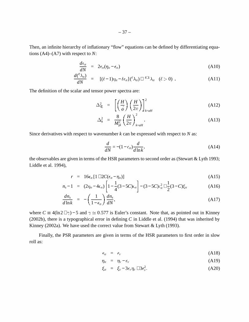
Then, an infinite hierarchy of inflationary “flow” equations can be defined by differentiating equa-tions (A4)–(A7) with respect to N:

d �H

dN= 2 �

H(�

H − �H) (A10)

d(� �

H)dN

= [( � − 1)�

H − � �H] (

� �H) +

�+1 �

H ( � � 0) � (A11)

The definition of the scalar and tensor power spectra are:� 2� = � � H� � � H2 � � � 2

k=aH

(A12)� 2h =

8M2

pl

� H2 � � 2

k=aH

� (A13)

Since derivatives with respect to wavenumber k can be expressed with respect to N as:

ddN

= −(1 − �H)

dd lnk

� (A14)

the observables are given in terms of the HSR parameters to second order as (Stewart & Lyth 1993;Liddle et al. 1994),

r = 16 �H [1 + 2C( �

H −�

H)] (A15)

ns − 1 = (2�

H − 4 �H) � 1 −

14

(3 − 5C) �H � − (3 − 5C) � 2

H +12

(3 −C)�

H (A16)

dns

d lnk= − � 1

1 − �H � dns

dN� (A17)

where C � 4(ln2 + � ) − 5 and � � 0 � 577 is Euler’s constant. Note that, as pointed out in Kinney(2002b), there is a typographical error in defining C in Liddle et al. (1994) that was inherited byKinney (2002a). We have used the correct value from Stewart & Lyth (1993).

Finally, the PSR parameters are given in terms of the HSR parameters to first order in slowroll as:

�H = �

V (A18)�H =

�V − �

V (A19)�

H =�

V − 3 �V

�V + 3 � 2

V � (A20)

– 38 –

REFERENCES

Adams, J., Cresswell, B., & Easther, R. 2001, Phys. Rev., D64, 123514

Adams, J. A., Ross, G. G., & Sarkar, S. 1997, Phys. Lett., B391, 271

Albrecht, A., Coulson, D., Ferreira, P., & Magueijo, J. 1996, Phys. Rev. Lett., 76, 1413

Albrecht, A. & Steinhardt, P. J. 1982, Phys. Rev. Lett., 48, 1220

Amendola, L., Gordon, C., Wands, D., & Sasaki, M. 2002, Phys. Rev. Lett., 88, 211302

Bardeen, J. M., Steinhardt, P. J., & Turner, M. S. 1983, Phys. Rev. D, 28, 679

Bartolo, N., Matarrese, S., & Riotto, A. 2001, Phys. Rev., D64, 123504

—. 2002, Phys. Rev., D65, 103505

Birrell, N. D. & Davies, P. C. W. 1982, Quantum fields in curved space (Cambridge UniversityPress)

Brans, C. & Dicke, R. H. 1961, Physical Review, 124, 925

Caprini, C., Hansen, S. H., & Kunz, M. 2003, MNRAS, 339, 212

Copeland, E. J., Liddle, A. R., Lyth, D. H., Stewart, E. D., & Wands, D. 1994, Phys. Rev., D49,6410

Croft, R. A. C., Weinberg, D. H., Bolte, M., Burles, S., Hernquist, L., Katz, N., Kirkman, D., &Tytler, D. 2002, ApJ, 581, 20

Dicke, R. H. 1962, Physical Review, vol. 125, Issue 6, pp. 2163-2167, 125, 2163

Dodelson, S., Kinney, W. H., & Kolb, E. W. 1997, Phys. Rev., D56, 3207

Durrer, R., Kunz, M., & Melchiorri, A. 2002, Phys. Rept., 364, 1

Dvali, G. R., Shafi, Q., & Schaefer, R. 1994, Phys. Rev. Lett., 73, 1886

Easther, R. & Kinney, W. H. 2002, Phys. Rev. D, submitted (astro-ph/0210345)

Garcia-Bellido, J. & Wands, D. 1996, Phys. Rev., D53, 5437

Gasperini, M. & Veneziano, G. 1993, Astropart. Phys., 1, 317

Gnedin, N. Y. & Hamilton, A. J. S. 2002, MNRAS, 334, 107

– 39 –

Gordon, C., Wands, D., Bassett, B. A., & Maartens, R. 2001, Phys. Rev., D63, 023506

Gratton, S., Khoury, J., Steinhardt, P., & Turok, N. 2003, preprint (astro-ph/0301395)

Guth, A. H. 1981, Phys. Rev. D, 23, 347

Guth, A. H. & Pi, S. Y. 1982, Phys. Rev. Lett., 49, 1110

Hannestad, S., Hansen, S. H., & Villante, F. L. 2001, Astroparticle Physics, 16, 137

Hansen, S. H. & Kunz, M. 2002, MNRAS, 336, 1007

Hawking, S. W. 1982, Phys. Lett., B115, 295

Hinshaw, G. F. et al. 2003, ApJ, submitted

Hoffman, M. B. & Turner, M. S. 2001, Phys. Rev., D64, 023506

Hu, W. & Sugiyama, N. 1995, ApJ, 444, 489

Hu, W. & White, M. 1996, ApJ, 471, 30

—. 1997, Phys. Rev. D, 56, 596

Hwang, J. & Noh, H. 1998, Physical Review Letters, Volume 81, Issue 24, December 14, 1998,pp.5274-5277, 81, 5274

Khoury, J., Ovrut, B. A., Seiberg, N., Steinhardt, P. J., & Turok, N. 2002, Phys. Rev., D65, 086007

Khoury, J., Ovrut, B. A., Steinhardt, P. J., & Turok, N. 2001, Phys. Rev., D64, 123522

Kinney, W. H. 1998, Phys. Rev., D58, 123506

—. 2002a, Phys. Rev., D66, 083508

—. 2002b, preprint (astro-ph/0206032)

Kogut, A. et al. 2003, ApJ, submitted

Komatsu, E. & Futamase, T. 1999, Phys. Rev., D59, 064029

Komatsu, E. et al. 2003, ApJ, submitted

Kuo, C. L. et al. 2002, ApJ, astro-ph/0212289

La, D. & Steinhardt, P. J. 1989, Phys. Rev. Lett., 62, 376

– 40 –

Langlois, D. 1999, Phys. Rev., D59, 123512

Langlois, D. & Riazuelo, A. 2000, Phys. Rev., D62, 043504

Leach, S. M., Liddle, A. R., Martin, J., & Schwarz, D. J. 2002, Phys. Rev. D, 66, 23515

Lewis, A., Challinor, A., & Lasenby, A. 2000, ApJ, 538, 473

Liddle, A. R. & Lyth, D. H. 1992, Phys. Lett., B291, 391

—. 1993, Phys. Rept., 231, 1

—. 2000, Cosmological inflation and large-scale structure (Cambridge University Press)

Liddle, A. R., Parsons, P., & Barrow, J. D. 1994, Phys. Rev., D50, 7222

Linde, A. D. 1982, Phys. Lett., B108, 389

—. 1983, Phys. Lett., B129, 177

—. 1990, Particle physics and inflationary cosmology (Chur, Switzerland: Harwood)

—. 1994, Phys. Rev., D49, 748

Linde, A. D. & Riotto, A. 1997, Phys. Rev., D56, 1841

Lyth, D. H. & Riotto, A. 1999, Phys. Rept., 314, 1

Magueijo, J., Albrecht, A., Coulson, D., & Ferreira, P. 1996, Phys. Rev. Lett., 76, 2617

Mukhanov, V. F. & Chibisov, G. V. 1981, JETP Letters, 33, 532

Mukhanov, V. F., Feldman, H. A., & Brandenberger, R. H. 1992, Phys. Rept., 215, 203

Mukherjee, P. & Wang, Y. 2003a, 1562, ApJ, submitted (astro-ph/0301562)

—. 2003b, 1058, ApJ, submitted (astro-ph/0301058)

Page, L. et al. 2003, ApJ, submitted

Parker, L. 1969, Phys. Rev., 183, 1057

Pearson, T. J., et al. 2002, ApJ, submitted (astro-ph/0205388)

Peebles, P. J. E. & Yu, J. T. 1970, ApJ, 162, 815

Pen, U.-L., Spergel, D. N., & Turok, N. 1994, Phys. Rev., D49, 692

– 41 –

Percival, W. J., et al. 2001, MNRAS, 327, 1297

Pierpaoli, E., Garcia-Bellido, J., & Borgani, S. 1999, Journal of High Energy Physics, 10, 15

Polarski, D. & Starobinsky, A. A. 1995, Phys. Lett., B356, 196

Sasaki, M. & Stewart, E. D. 1996, Prog. Theor. Phys., 95, 71

Sato, K. 1981, MNRAS, 195, 467

Seljak, U., Pen, U.-L., & Turok, N. 1997, Phys. Rev. Lett., 79, 1615

Seljak, U. & Zaldarriaga, M. 1996, ApJ, 469, 437

Spergel, D. N. & Zaldarriaga, M. 1997, Phys. Rev. Lett., 79, 2180

Spergel, D. N. et al. 2003, ApJ, submitted

Starobinsky, A. A. 1982, Phys. Lett., B117, 175

Stewart, E. D. & Lyth, D. H. 1993, Phys. Lett., B302, 171

Tsujikawa, S., Brandenberger, R., & Finelli, F. 2002, Phys. Rev. D, 66, 83513

Turok, N. 1996a, Phys. Rev. Lett., 77, 4138

—. 1996b, ApJ, 473, L5

Turok, N., Pen, U.-L., & Seljak, U. 1998, Phys. Rev., D58, 023506

Verde, L. et al. 2003, ApJ, submitted

Wands, D., Bartolo, N., Matarrese, S., & Riotto, A. 2002, Phys. Rev., D66, 043520

Wang, Y., Spergel, D. N., & Strauss, M. A. 1999, ApJ, 510, 20

Zaldarriaga, M. & Harari, D. D. 1995, Phys. Rev., D52, 3276

This preprint was prepared with the AAS LATEX macros v5.0.

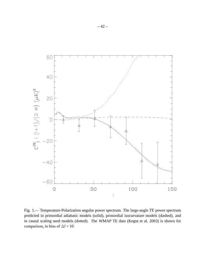
– 42 –

Fig. 1.— Temperature-Polarization angular power spectrum. The large-angle TE power spectrumpredicted in primordial adiabatic models (solid), primordial isocurvature models (dashed), andin causal scaling seed models (dotted). The WMAP TE data (Kogut et al. 2003) is shown forcomparison, in bins of

�l = 10.

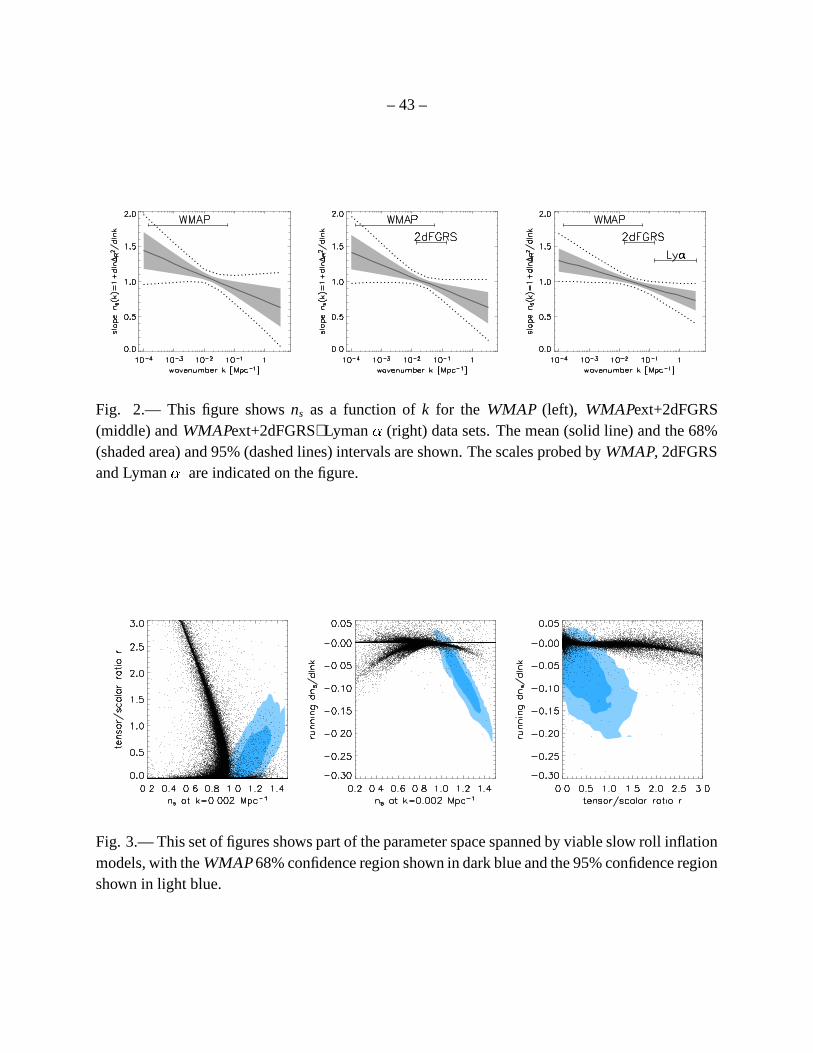
– 43 –

Fig. 2.— This figure shows ns as a function of k for the WMAP (left), WMAPext+2dFGRS(middle) and WMAPext+2dFGRS+Lyman � (right) data sets. The mean (solid line) and the 68%(shaded area) and 95% (dashed lines) intervals are shown. The scales probed by WMAP, 2dFGRSand Lyman � are indicated on the figure.

Fig. 3.— This set of figures shows part of the parameter space spanned by viable slow roll inflationmodels, with the WMAP 68% confidence region shown in dark blue and the 95% confidence regionshown in light blue.

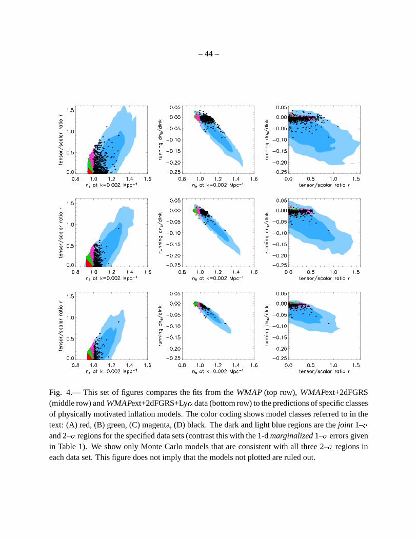
– 44 –

Fig. 4.— This set of figures compares the fits from the WMAP (top row), WMAPext+2dFGRS(middle row) and WMAPext+2dFGRS+Ly � data (bottom row) to the predictions of specific classesof physically motivated inflation models. The color coding shows model classes referred to in thetext: (A) red, (B) green, (C) magenta, (D) black. The dark and light blue regions are the joint 1– �and 2– � regions for the specified data sets (contrast this with the 1-d marginalized 1– � errors givenin Table 1). We show only Monte Carlo models that are consistent with all three 2– � regions ineach data set. This figure does not imply that the models not plotted are ruled out.

– 45 –

Fig. 5.— This set of figures compares the fits from the WMAPext+2dFGRS+Ly � data to thepredictions of all four classes of inflation models. The top row is Class A [red dots]. The sec-ond row is Class B [green dots]. The third row is Class C [magenta dots]. The bottom row isClass D [black dots]. The dark and light blue regions are the joint 1– � and 2– � regions for theWMAPext+2dFGRS+Ly � data. We show only Monte Carlo models that are consistent with 2– �regions in all panels. This figure does not imply that the models not plotted are ruled out.

– 46 –

Fig. 6.— The cumulative distribution of the isocurvature fraction, fiso, for theWMAPext+2dFGRS+Lyman � data set.

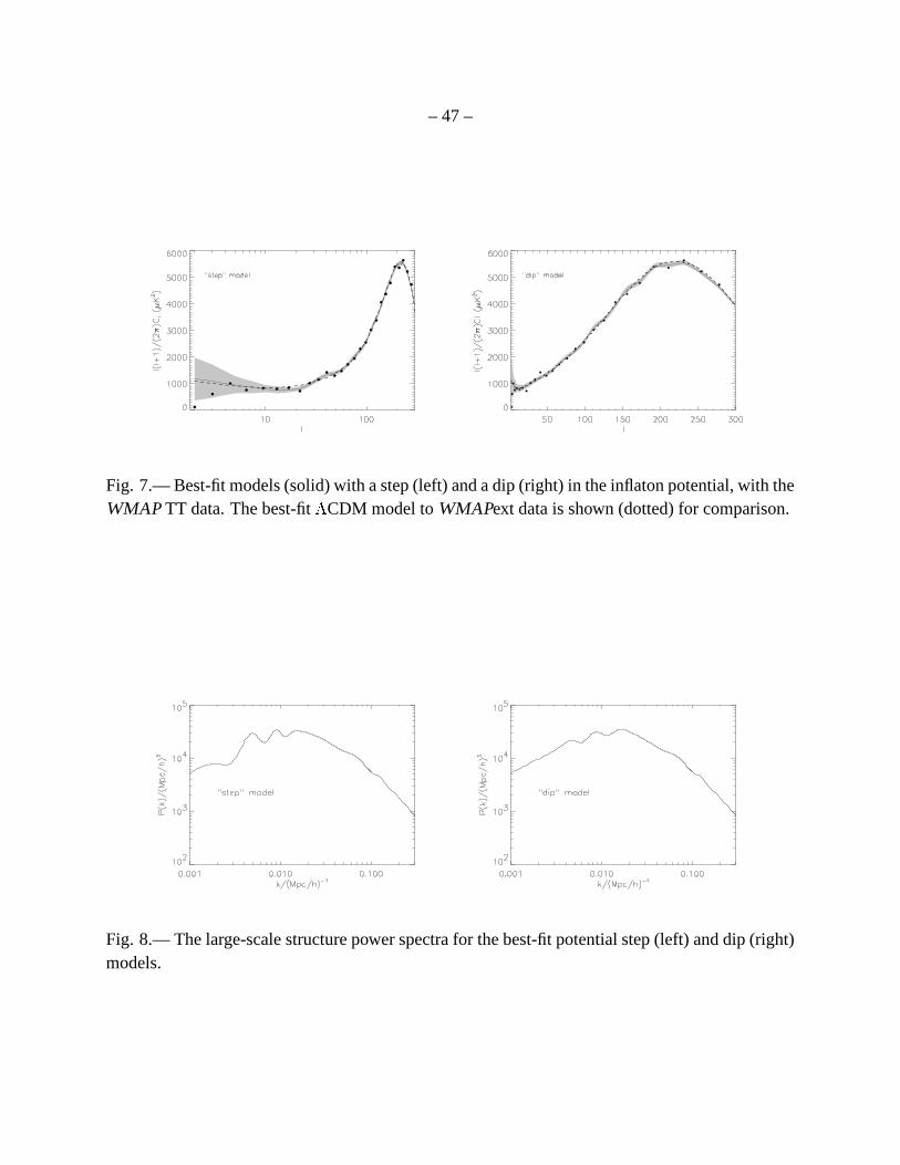
– 47 –

Fig. 7.— Best-fit models (solid) with a step (left) and a dip (right) in the inflaton potential, with theWMAP TT data. The best-fit � CDM model to WMAPext data is shown (dotted) for comparison.

Fig. 8.— The large-scale structure power spectra for the best-fit potential step (left) and dip (right)models.

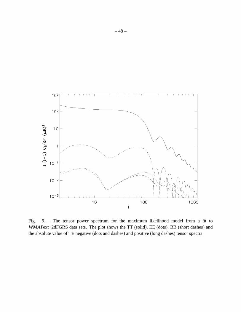
– 48 –

Fig. 9.— The tensor power spectrum for the maximum likelihood model from a fit toWMAPext+2dFGRS data sets. The plot shows the TT (solid), EE (dots), BB (short dashes) andthe absolute value of TE negative (dots and dashes) and positive (long dashes) tensor spectra.