FIRST-PRINCIPLES STUDY OF MAGNETOELECTRIC EFFECTS AND

FIRST-PRINCIPLES STUDY OFMAGNETOELECTRIC EFFECTS AND

FERROELECTRICITY IN COMPLEX OXIDES

BY MENG YE

A dissertation submitted to the

Graduate School—New Brunswick

Rutgers, The State University of New Jersey

in partial fulfillment of the requirements

for the degree of

Doctor of Philosophy

Graduate Program in Physics and Astronomy

Written under the direction of

Professor David Vanderbilt

and approved by

New Brunswick, New Jersey

October, 2016

ABSTRACT OF THE DISSERTATION

First-principles study of magnetoelectric effects and

ferroelectricity in complex oxides

by Meng Ye

Dissertation Director: Professor David Vanderbilt

This thesis contains several investigations of magnetoelectric effects and ferroelectricity

in complex oxides studied via first-principles calculations. We start by reviewing the

mechanisms of ferroelectricity and magnetoelectric effects, and then we give a brief in-

troduction to the first-principles computational methods that are involved. Next, our

investigations are divided into two parts. The first half focuses on the magnetoelectric

effects, while the second half is mainly on ferroelectricity. The first half aims to ex-

amine the lattice contribution to the magnetoelectricity by investigating the dynamical

magnetic charge tensors induced by different mechanisms. Through the study of Cr2O3

and a fictitious material KITPite, we find that the dynamical magnetic charges driven

by exchange striction are more significant than the ones induced by spin-orbit coupling.

Since the lattice contribution to the magnetoelectric effect is proportional to the dy-

namical magnetic charges, we also study the magnetic charges and the magnetoelectric

coupling in hexagonal manganite RMnO3 and ferrite RFeO3. Our results further con-

firm the importance of the exchange-striction mechanism in inducing large magnetic

ii

charges, but we also notice that the magnetoelectric contributions from various phonons

tend to cancel each other, leading to a great reduction of the total coupling. These in-

vestigations not only provide a prediction of the magnetoelectric coupling constant in

RMnO3 and RFeO3, but also emphasize the importance of phonons in magnetoelectric

coupling. In the second half of the thesis, we focus on predicting new ferroelectrics

in the family of corundum derivatives. Many new corundum derivatives have been

synthesized recently; these are automatically polar, and many are magnetic as well.

However, a polar material is only called ferroelectric if the polarization is reversible by

an external field, and it is not yet clear whether or not this is the case for these new

materials. Motivated by this question, we use a structural constraint method to study

the ferroelectric reversal path and energy barrier of several corundum derivatives. As

a result, we predict several FE candidates with insulting reversal paths and low barrier

energies. Since the hysteresis behavior of ferroelectrics is attributed to the ferroelectric

domain wall motion, we further investigate the formation and motion of ferroelectric

domain walls in corundum derivatives. Our study predicts the atomic structure and ori-

entation of the ferroelectric domain wall, as well as the shape of ferroelectric domains.

In addition, we find novel properties at domain walls, including a strong magnetoelec-

tric coupling and an interlocking between chirality and polarization. Moreover, we use

the structural constraint method to study the barrier energy of ferroelectric domain

wall reversal. Our results suggest that the barrier energy is linearly correlated with the

bond valence sum, which can be used as a guide to find new ferroelectrics in the family

of corundum derivatives.

iii

Acknowledgements

I still remember the first day I came to Rutgers five years ago. I still have the receipt

of the one-way flight from China to Newark, New Jersey. After five years, Rutgers,

11 thousand kilometers away from my hometown, has become a home away from my

home. Five years is not a long time compared with one’s lifetime, but this five years is

definitely unforgettable. In this five years, I lived in a different country, I got married,

and I got my Ph.D in physics. There are many people in my mind that I want to

acknowledge.

Han Yu, a Chinese essayist and poet from the Tang dynasty, said “A teacher is

one who transmits knowledge, provides for study and dispels confusion.” This is an

accurate depiction of my advisor Professor David Vanderbilt. He is always willing to

teach me from scratch and answer my endless questions. His rigorous, modest, gentle,

and professional attitudes guided me from every aspect about how to be a physicist and

a respectful person. I not only appreciate all his contributions of time, creative ideas,

and funding support, but also that he gave enough trust and freedom to me to explore

on my own direction and at my own pace. He encouraged and supported me to attend

many workshops, symposiums, and conferences, which gradually led me to be a good

speaker and listener. I am so thankful that I have Professor David Vanderbilt as my

advisor, who makes my Ph.D. experience productive, joyful, and stimulating.

I thank my committee members Professor Jane Hinch, Professor Charles Keeton,

Professor Premala Chandra, and my outside committee member Professor Ismaila Dabo

from Penn State. Their questions and active feedback deepened my understanding.

I also want to thank Professor Karin Rabe for her thought-provoking and inspiring

questions and suggestions. The big smile on her face and her excitement towards new

and bold ideas left deep impressions on me.

iv

It was a very pleasant experience to collaborate with Professor Martha Greenblatt

and Dr. Manrong Li. I feel fortunate that they introduced the interesting materials,

the corundum derivatives, to me. Each interaction with them taught me to think about

the physical problems from different perspectives.

My sincere thanks also go to Professor Sang-Wook Cheong for his inspiration and

advice. In the last year of my Ph.D. program, I had many interactions with him and he

greatly motivated me to learn more from experimentalists. His advices will be a great

treasure for my future research.

I want to express my gratitude to Professor Weida Wu. He is very gentle, patient,

and knowledgeable. I learned a lot about experiments as well as theories from him.

I want to give special thanks to Professor Premala Chandra and her efforts in the

organization of “Women’s Lunch” activities. I thank all the attendees of “Women’s

Lunch” for sharing their stories of personal lives and academic careers. Their advices

and encouragements will accompany me through different stages of my life.

I would like to express my appreciation to Professor Jolie Cizewski. I have worked as

a teaching assistant in her courses for several semesters and I have helped her proctoring

many exams. Her rigorous attitude towards teaching and her endless efforts to achieve

fairness will guide me to be a responsible teacher.

Confucian said,“When I walk along with two others, they may serve me as my teach-

ers”. My thanks go to the postdoc fellows, graduate students at Rutgers, including

Jianpeng Liu, Maryam Taherinejad, Yuanjun Zhou, Sebastian Reyes-Lillo, Qibin Zhou,

John Bonini, Bartomeu Monserrat, Cyrus Dreyer, Michele Kotiuga, Xiaohui Liu, Jialan

Zhang, Se Young Park, Turan Birol, Hongbin Zhang, Sergey Artyukhin, Joseph Ben-

nett, Huaqing Huang, Andrei Malashevich, Fei-Ting Huang, Yazhong Wang, Xueyun

Wang, Wenbo Wang, Wenhan Zhang, Shuchen Zhu, Qiang Han, Yanan Geng, Jae Wook

Kim, Juho Lee, Chris Munson, Huijie Guan, Wenhu Xu, Wenshuo Liu, Can Xu, Jian-

guo Xiao, and Xukai Yan. I benefitted a lot from the enlightening discussion with them

and they enriched my graduate life.

I cannot thank more for my husband Mohan Chen. He has made great efforts to

come across the Pacific to Princeton and accompanied me for four years. We have

v

embraced the beauty of cherry blossom in the spring and have chased the foliage in the

fall. We together have faced a winter storm in May and we have marched in the desert

when all the families were enjoying turkeys and pumpkins. I like adventures because

Mohan is always by my side to back me up. I hope our adventures in physics would

last forever.

In the end, I would like to express my gratitude to my family. Although we are

11 thousand kilometers apart, we still share the same joy, sorrow, and the clear bright

moonlight on Mid-Autumn Day.

vi

Dedication

to Jianjian and his friends for their company days and nights

vii

Table of Contents

Abstract . . . . . . . . . . . . . . . . . . . . . . . . . . . . . . . . . . . . . . . . ii

Acknowledgements . . . . . . . . . . . . . . . . . . . . . . . . . . . . . . . . . iv

Dedication . . . . . . . . . . . . . . . . . . . . . . . . . . . . . . . . . . . . . . . vii

List of Tables . . . . . . . . . . . . . . . . . . . . . . . . . . . . . . . . . . . . . xi

List of Figures . . . . . . . . . . . . . . . . . . . . . . . . . . . . . . . . . . . . xv

1. Introduction . . . . . . . . . . . . . . . . . . . . . . . . . . . . . . . . . . . 1

1.1. Motivations . . . . . . . . . . . . . . . . . . . . . . . . . . . . . . . . . . 1

1.2. Ferroelectricity . . . . . . . . . . . . . . . . . . . . . . . . . . . . . . . . 3

1.2.1. General properties . . . . . . . . . . . . . . . . . . . . . . . . . . 3

1.2.2. Ferroelectric phase transition . . . . . . . . . . . . . . . . . . . . 5

1.2.3. Soft modes and boundary conditions . . . . . . . . . . . . . . . . 7

1.2.4. Beyond the soft-mode ferroelectricity . . . . . . . . . . . . . . . . 9

1.3. Magnetoelectricity and multiferroicity . . . . . . . . . . . . . . . . . . . 10

1.3.1. Brief history . . . . . . . . . . . . . . . . . . . . . . . . . . . . . 10

1.3.2. Mechanisms . . . . . . . . . . . . . . . . . . . . . . . . . . . . . . 13

1.4. Outline of the present work . . . . . . . . . . . . . . . . . . . . . . . . . 15

2. Computational methods . . . . . . . . . . . . . . . . . . . . . . . . . . . . 18

2.1. Density functional theory . . . . . . . . . . . . . . . . . . . . . . . . . . 19

2.1.1. Kohn-Sham equations . . . . . . . . . . . . . . . . . . . . . . . . 19

2.1.2. Exchange-correlation functionals . . . . . . . . . . . . . . . . . . 20

2.1.3. On-site Coulomb correction . . . . . . . . . . . . . . . . . . . . . 21

2.1.4. Practical implementations . . . . . . . . . . . . . . . . . . . . . . 21

viii

2.2. Phonons . . . . . . . . . . . . . . . . . . . . . . . . . . . . . . . . . . . . 22

2.3. Modern theory of polarization . . . . . . . . . . . . . . . . . . . . . . . . 23

3. Dynamical magnetic charges and magnetoelectric effects . . . . . . . 29

3.1. Introduction . . . . . . . . . . . . . . . . . . . . . . . . . . . . . . . . . . 29

3.2. Formalism . . . . . . . . . . . . . . . . . . . . . . . . . . . . . . . . . . . 31

3.3. Structure and symmetry . . . . . . . . . . . . . . . . . . . . . . . . . . . 36

3.3.1. Cr2O3 . . . . . . . . . . . . . . . . . . . . . . . . . . . . . . . . . 36

3.3.2. KITPite . . . . . . . . . . . . . . . . . . . . . . . . . . . . . . . . 36

3.4. First-principles methodology . . . . . . . . . . . . . . . . . . . . . . . . 38

3.5. Results and discussion . . . . . . . . . . . . . . . . . . . . . . . . . . . . 39

3.5.1. Structure and phonon . . . . . . . . . . . . . . . . . . . . . . . . 39

3.5.2. Born charge . . . . . . . . . . . . . . . . . . . . . . . . . . . . . . 40

3.5.3. Magnetic charge . . . . . . . . . . . . . . . . . . . . . . . . . . . 41

3.5.4. Electric and magnetic responses . . . . . . . . . . . . . . . . . . 42

3.6. Summary and outlook . . . . . . . . . . . . . . . . . . . . . . . . . . . . 44

4. Magnetoelectric effects in hexagonal rare-earth manganites and fer-

rites . . . . . . . . . . . . . . . . . . . . . . . . . . . . . . . . . . . . . . . . . . . 45

4.1. Introduction . . . . . . . . . . . . . . . . . . . . . . . . . . . . . . . . . . 45

4.2. Preliminary . . . . . . . . . . . . . . . . . . . . . . . . . . . . . . . . . . 47

4.2.1. Structure and magnetic phase . . . . . . . . . . . . . . . . . . . . 47

4.2.2. Symmetry analysis . . . . . . . . . . . . . . . . . . . . . . . . . 49



4.4.1. Born charge and force-constant matrix . . . . . . . . . . . . . . . 52

4.4.2. Magnetization and magnetic charge . . . . . . . . . . . . . . . . 52

4.4.3. Magnetoelectric effect . . . . . . . . . . . . . . . . . . . . . . . . 57


ix

5. Ferroelectricity in corundum derivatives . . . . . . . . . . . . . . . . . . 62

5.1. Introduction . . . . . . . . . . . . . . . . . . . . . . . . . . . . . . . . . . 62

5.2. Preliminary . . . . . . . . . . . . . . . . . . . . . . . . . . . . . . . . . . 64

5.2.1. Structure . . . . . . . . . . . . . . . . . . . . . . . . . . . . . . . 64

5.2.2. Coherent ferroelectric reversal . . . . . . . . . . . . . . . . . . . . 65

5.2.3. Energy profile calculation . . . . . . . . . . . . . . . . . . . . . . 67



5.4.1. Ground state structure and magnetic order . . . . . . . . . . . . 70

5.4.2. Symmetry of the reversal path . . . . . . . . . . . . . . . . . . . 72

5.4.3. Polarization reversal barrier . . . . . . . . . . . . . . . . . . . . . 76

5.4.4. Insulating vs conducting . . . . . . . . . . . . . . . . . . . . . . . 80

5.4.5. More complicated magnetic structures . . . . . . . . . . . . . . . 82

5.4.6. Hyperferroelectric? . . . . . . . . . . . . . . . . . . . . . . . . . . 84


6. Ferroelectric and magnetoelectric domain walls in corundum deriva-

tives . . . . . . . . . . . . . . . . . . . . . . . . . . . . . . . . . . . . . . . . . . . 87

6.1. Introduction . . . . . . . . . . . . . . . . . . . . . . . . . . . . . . . . . . 87



6.3.1. Construction of domain walls . . . . . . . . . . . . . . . . . . . . 89

6.3.2. Orientation of domain walls . . . . . . . . . . . . . . . . . . . . . 92

6.3.3. Magnetic and magnetoelectric domain walls . . . . . . . . . . . . 94

6.3.4. Domain wall reversal . . . . . . . . . . . . . . . . . . . . . . . . . 98


7. Conclusion and outlook . . . . . . . . . . . . . . . . . . . . . . . . . . . . 105

References . . . . . . . . . . . . . . . . . . . . . . . . . . . . . . . . . . . . . . . 108

x

List of Tables

3.1. Structural parameters of Cr2O3 from first-principles calculation and ex-

periments: rhombohedral lattice constant a, lattice angle α, and Wyckoff

positions for Cr (4c) and O (6e). . . . . . . . . . . . . . . . . . . . . . . 39

3.2. Frequencies (cm−1) of IR-active phonon modes of Cr2O3 from first-

principles calculations and experiments. The two A2u modes are at longi-

tudinal direction; the four Eu modes are at transverse direction (doubly

degenerate). . . . . . . . . . . . . . . . . . . . . . . . . . . . . . . . . . . 40

3.3. Magnetic charges Zm (10−2µB/A) for Cr2O3 in the atomic basis. . . . 41

3.4. Magnetic charges Zm (10−2µB/A) for KITPite CaAlMn3O7 in atomic

basis. . . . . . . . . . . . . . . . . . . . . . . . . . . . . . . . . . . . . . 42

3.5. Top: Mode decomposition of the Born charges Ze, and of the spin and

orbital contributions to the magnetic charges Zm, in Cr2O3. Cn are

the eigenvalues of the force-constant matrix. Bottom: Total A2u-mode

(longitudinal) and Eu-mode (transverse) elements of the lattice-mediated

electric susceptibility χe, magnetic susceptibility χm, and the spin and

orbital parts of the ME constant α. . . . . . . . . . . . . . . . . . . . . . 43

3.6. Born charges Ze and magnetic charges Zm for IR-active A2u modes in

CaAlMn3O7. Cn are the eigenvalues of the force-constant matrix. . . . . 43

4.1. Symmetry patterns of Born charges Ze, magnetic charges Zm and ME

tensors α in RMnO3 and RFeO3. Patterns for Mn, Fe, OT1, and OT2

are for atoms lying on an My mirror plane. Unless otherwise specified,

patterns apply to both A1 and A2 phases. . . . . . . . . . . . . . . . . . 50

4.2. Atomic Born charge tensors Ze (in units of |e|) for RMnO3 and LuFeO3

in the A2 phase. TM = Mn, Fe. . . . . . . . . . . . . . . . . . . . . . . . 53

xi

4.3. Eigenvalues of the force-constants matrix (eV/A2) for IR-active modes

in RMnO3 and LuFeO3 in the A2 phase, and for HoMnO3 in the A1 phase 54

4.4. Longitudinal magnetic charge components Zm (10−3 µB/A) of RMnO3

and LuFeO3 in the A2 phase. All components vanish in the absence of

SOC. . . . . . . . . . . . . . . . . . . . . . . . . . . . . . . . . . . . . . . 55

4.5. Transverse magnetic charge components Zm (10−2 µB/A) of HoMnO3 in

the A1 phase, as computed including or excluding SOC. . . . . . . . . . 56

4.6. Transverse magnetic charge components Zm (10−2 µB/A) of RMnO3 and

LuFeO3 in the A2 phase, as computed including or excluding SOC. . . . 57

4.7. Computed ME couplings αzz (longitudinal) and αxx and αyx (transverse)

for RMnO3 and LuFeO3 (ps/m). Spin-lattice, spin-electronic, and total

spin couplings are given as computed with and without SOC. . . . . . . 58

4.8. Transverse ME contributions (ps/m) from IR-active modes for A2 and

A1 phases of HoMnO3 and A2 phase of LuMnO3. Results are given

in ascending order of force-constant eigenvalues, which are reported in

Table 4.3. . . . . . . . . . . . . . . . . . . . . . . . . . . . . . . . . . . . 60

5.1. Corundum-derived structures before and after polarization reversal. . . 66

5.2. Rhombohedral structural parameters of LNO-typeABO3 corundum deriva-

tives LiNbO3, LiTaO3, ZnSnO3, FeTiO3 and MnTiO3 from our first-

principles calculations and experiments [111, 127, 128, 129, 130]. The

Wyckoff positions are 2a for A and B cations, and 6c for oxygen anions

(note that Ax = Ay = Az and Bx = By = Bz). The origin is defined by

setting the Wyckoff position Bx to zero. . . . . . . . . . . . . . . . . . . 69

xii

5.3. Rhombohedral structure parameters of ordered-LNOA2BB′O6corundum

derivatives Li2ZrTeO6, Li2HfTeO6, Mn2FeWO6, Mn3WO6 and Zn2FeOsO6

from our first-principles calculations and experiments [115, 44]. Wyckoff

positions are 1a for A1, A2, B and B′ cations, and 3b for O1 and O2

anions. The origin is defined by setting the Wyckoff position B′x to zero.

For ordered-LNO Li2HfTeO6 and Zn2FeOsO6, no experimental results

are available. Magnetic orders used in the calculation for Mn2FeWO6,

Mn3WO6, and Zn2FeOsO6 are also indicated by “Mag”. . . . . . . . . . 69

5.4. Oxidation states of the LNO-type ABO3 and the ordered-LNO A2BB′O6

corundum derivatives. The oxidation state of O ion is −2 in all materials. 70

5.5. Magnetic energy of different magnetic states relative to the lowest-energy

state in Mn2FeWO6 and Mn3WO6, in units of meV per unit cell. . . . . 71

5.6. Relative spin direction between different magnetic ions in Mn2FeWO6

and Mn3WO6. Here “FM” means ferromagnetic. . . . . . . . . . . . . . 72

5.7. Energy and unstable phonon modes at the midpoint structure of LiNbO3,

LiTaO3, ZnSnO3, FeTiO3 and MnTiO3 with symmetry R3c and R3. The

energy of the ground-state structure is set to be zero as reference and

the unit is meV per unit cell. The imaginary frequency of the unstable

phonon is given in units of cm−1. . . . . . . . . . . . . . . . . . . . . . . 73

5.8. Coherent polarization reversal barrier Ebarrier (meV) per unit cell and

spontaneous polarization PS (µC/cm2) for FE candidates. . . . . . . . . 77

5.9. Midpoint structures of ordered-LNO candidates and the energy differ-

ences between B and B′ sandwiched midpoint structures. The distances

between A1 (or A2) cation and the oxygen planes in the ground state

are characterized by ξ1S (or ξ2S). The energy difference between the B

and B′ sandwiched midpoint structures is ∆E. The Madelung energy

difference between the B and B′ sandwiched midpoint structures is ∆EM. 78

xiii

5.10. Magnetic energies for AFM doubled-cell magnetic structures. ∆E1 is for

energies evaluated at the unrelaxed experimental structure, while ∆E2

applies to energies calculated after relaxation of the internal coordinates.

The energy is given with respect to the udu magnetic order in the ex-

perimental cell with unit meV/f.u. . . . . . . . . . . . . . . . . . . . . . 83

5.11. . . . . . . . . . . . . . . . . . . . . . . . . . . . . . . . . . . . . . . . . . 84

6.1. Formation energy of X-wall and Y-wall. For the ordered-LNO structure,

the formation energy is averaged between the DW⇑⇓ and DW⇓⇑. The

unit is mJ/m2. . . . . . . . . . . . . . . . . . . . . . . . . . . . . . . . . 94

6.2. DW-mediated polarization reversal barrier Ebarrier for corundum deriva-

tives. The energy barriers of DW⇑⇓ and DW⇓⇑ are the same in LNO-type

structures, but different in ordered-LNO structure. The unit of Ebarrier

is meV per unit cell. . . . . . . . . . . . . . . . . . . . . . . . . . . . . . 100

xiv

List of Figures

1.1. The cross coupling between polarization, magnetization, and strain. The

electric field E, magnetic field H, and stress σ control the electric po-

larization P, magnetization M, and strain ε, respectively. This figure is

taken from [2]. . . . . . . . . . . . . . . . . . . . . . . . . . . . . . . . . 2

1.2. Relationship between dielectric,piezoelectric, pyroelectric and ferroelectric. 3

1.3. Sketch of P-E relation of (a) a dielectric and (b) a FE. (c) The first FE

hysteresis loop of rochelle salt taken from Ref. [1]. . . . . . . . . . . . . 4

1.4. PE-FE phase transition described by the Landau-Ginzburg-Devonshire

theory. (a) Free energy as a function of polarization in the vicinity of Tc

in the absent of an external electric field. (b) Free energy as a function

of polarization in the FE phase at various electric fields. (c) Evolution

of polarization as a function of an external electric field at various of

temperatures. Hysteresis loop 1-2-3-1′-2′-3′ is observed in the FE phase. 6

1.5. The FE structure (a) and the centrosymmetric reference structure (b)

of PbTiO3. The arrow in (b) represent the magnitude of the atomic

displacement in the unstable polar mode, where the position of Pb cation

is fixed as the origin. . . . . . . . . . . . . . . . . . . . . . . . . . . . . . 7

1.6. (a) E = 0 and (b) D = 0 boundary conditions for FEs. . . . . . . . . . 9

1.7. Publication per year with keyword “magnetoelectric” according to the

Web of Science . . . . . . . . . . . . . . . . . . . . . . . . . . . . . . . . 12

1.8. Dzyaloshinskii-Moriya interaction. The open red circle represents oxygen

ion. The filled blue circle and filled blue arrow are magnetic ion and its

spin. . . . . . . . . . . . . . . . . . . . . . . . . . . . . . . . . . . . . . . 14

xv

1.9. Exchange-striction interaction. (a) The cation-anion-cation bond with-

out external fields. (b) The cation-anion-cation bond in the presence of

an electric field. The open red circle represents oxygen ion. The filled

blue circle and filled blue arrow are magnetic ion and its spin. . . . . . 15

2.1. A 1D chain of alternating anions and cations. The distance between each

anion and cation is a/2. The two dashed rectangles indicate two different

choices of unit cell. . . . . . . . . . . . . . . . . . . . . . . . . . . . . . . 24

2.2. An experimental setup to measure the spontaneous polarization in fer-

roelectric materials. The ferroelectric sample is inserted into a shorted

capacitor. Free charges are accumulated on top and bottom of the ca-

pacitor to screen out the bulk polarization. When the bulk polarization

is reversed from (a) to (b) by an electric field, current flows through the

ammeter in the shorted wire to re-screen the bulk polarization. . . . . . 25

2.3. Polarization as a function of λ. The formal polarization is a multivalued

quantity and at a certain λ value, the polarization in different branches

differ by an integer times the polarization quantum PQ. Within each

path, the polarization stays on the same branch and changes continuously. 28

3.1. Sketch for different contributions to magnetoelectric effect. (a) The high

symmetry system under no external field. (b) The electronic, (c) ionic,

and (d) strain-mediated contributions. The small blue circle represents

ion, the large red oval represents electron cloud, and the black outline

represents the unit cell. . . . . . . . . . . . . . . . . . . . . . . . . . . . 29

3.2. Sketch showing how the six lattice-mediated responses indicated by solid

circles are built up from the four elementary tensors indicated by open

circles: the Born charge Ze, magnetic charge Zm, internal strain Λ, and

force-constant inverse K−1. Each lattice-mediated response is given by

the product of the three elementary tensors connected to it, as indicated

explicitly in Eqs. (3.11-3.16). . . . . . . . . . . . . . . . . . . . . . . . . 34

xvi

3.3. Structure of Cr2O3. (a) In the primitive cell, four Cr atoms align along

the the rhombohedral axis with AFM order represented by the arrows

on Cr atoms. (b) Each Cr atom is at the center of a distorted oxygen

octahedron. . . . . . . . . . . . . . . . . . . . . . . . . . . . . . . . . . . 35

3.4. Symmetry pattern of Born and magnetic charge tensors for (a) the

Cr atom in Cr2O3, (b) the O atom in Cr2O3 and the O2 atom in

CaAlMn3O7, (c) the Ca, Al and O1 atoms in CaAlMn3O7, and (d) the

Mn and O3 atoms in CaAlMn3O7. The elements indicated by an asterisk

vanish in the absence of SOC for Zm in CaAlMn3O7. . . . . . . . . . . . 36

3.5. Planar view of the CaAlMn3O7 (KITPite) structure. The broad arrows

(blue) on the Mn atoms represent the magnetic moment directions in

the absence of electric or magnetic fields. Small (black) arrows indicate

the atomic forces induced by an external magnetic field applied in the y

direction. . . . . . . . . . . . . . . . . . . . . . . . . . . . . . . . . . . . 37

4.1. Structure of ferroelectric hexagonal RMnO3 or RFeO3 (6 f.u. per prim-

itive cell). (a) Side view from [110]. (b) Plan view from [001]; dashed

(solid) triangle indicates three Mn3+ or Fe3+ connected via Op1 to form

a triangular sublattice at z = 0 (z = 1/2). . . . . . . . . . . . . . . . . . 48

4.2. Magnetic phases of hexagonal RMnO3 and RFeO3. Mn3+ or Fe3+ ions

form triangular sublattices at z = 0 (dash line) and z = 1/2 (solid line).

(a) A2 phase with magnetic symmetry P63c′m′; spins on a given Mn3+

layer point all in or all out. (b) A1 phase with the magnetic symmetry

P63cm, with Mn3+ spins pointing tangentially to form a vortex pattern.

The A1 and A2 phases differ by a 90 global rotation of spins. The B1

and B2 phases can be obtained from A2 and A1 by reversing the spins

on the dashed triangles. . . . . . . . . . . . . . . . . . . . . . . . . . . . 49

4.3. Transverse ME couplings αxx for A2 phase RMnO3 and LuFeO3, and

αyx for A1 phase HoMnO3. (a) Spin-lattice; (b) spin-electronic; and (c)

total spin couplings. The unit is ps/m. . . . . . . . . . . . . . . . . . . . 59

xvii

5.1. Structures of (a) a cubic perovskite ABO3 and (b) a double perovskite

A2BB′O6. . . . . . . . . . . . . . . . . . . . . . . . . . . . . . . . . . . . 63

5.2. Structure of corundum derivatives. The unit cell in the rhombohedral

setting is shown at the left; an enlarged hexagonal-setting view is shown

at right. The cations α, β, γ, and δ are are all identical in the X2O3

corundum structure. For the LNO-type ABO3, β = δ = A, α = γ = B;

for the ilmenite ABO3, β = γ = A, α = δ = B; for the ordered-

LNO A2BB′O6, β = δ = A, γ = B, α = B′; for the ordered-ilmenite

A2BB′O6, β = γ = A, δ = B, α = B′. At left, ξ1 (or ξ2) is the distance

between β (or δ) and the oxygen plane that it penetrates during the

polarization reversal. . . . . . . . . . . . . . . . . . . . . . . . . . . . . . 65

5.3. Movements of A cations in LNO-type (red, here LiNbO3) and ordered-

LNO (blue, here Mn2FeWO6) corundum derivatives along the polariza-

tion reversal path. ξ1 and ξ2 are the distances from A atoms to the

oxygen planes that are penetrated during the polarization reversal, here

rescaled to a range between −1 and 1. The symmetry at an arbitrary

(ξ1, ξ2) point is R3; on the ξ1 = ξ2 and ξ1 =−ξ2 diagonals it is raised to

R3c and R3, respectively; and at the origin (ξ1 = ξ2 =0) it reaches R3c.

Green diamonds denote the midpoint structure in the parameter space.

In the LNO-type case “path1” and “path2” (filled and open red square

symbols) are equivalent and equally probable, while the ordered-LNO

system deterministically follows “path1” (full blue line), which becomes

“path2” (dashed blue) under a relabeling ξ1 ↔ ξ2. . . . . . . . . . . . . 74

5.4. Structural evolution along the polarization reversal path of LNO-type

and ordered-LNO corundum derivatives. “Before” and “After” are the

initial and final structures on the reversal path with symmetry R3c

for the LNO-type and R3 for the ordered-LNO corundum derivatives;

“Midpoint” denotes the structure halfway between these and exhibits

R3 structural symmetry in both cases. . . . . . . . . . . . . . . . . . . . 75

xviii

5.5. Polarization reversal energy profile for LiNbO3, LiTaO3, Mn2FeWO6,

Zn2FeOsO6, and Li2ZrTeO6. . . . . . . . . . . . . . . . . . . . . . . . . 76

5.6. Empirical proportionality between the coherent FE energy barrier and

P 2S . The red curve is the fitting polynomial Ebarrier = (µ/2)P 2

S , with

µ/2 = 0.057 meVcm4/µC2. . . . . . . . . . . . . . . . . . . . . . . . . . . 79

5.7. Empirical correlation between the spontaneous polarization and the re-

action coordinate ξ in the ground state. The red curve is the fitting

polynomial PS = mξS + nξ3S with m = 13.3 × 108 µC/cm3 and n =

19.0× 1024 µC/cm5. . . . . . . . . . . . . . . . . . . . . . . . . . . . . . 79

5.8. Energy profile and bandgap at the polarization reversal path of FeTiO3.

The band gap is 1.56 eV and 0.98 eV at points a and c, but FeTiO3 is

conducting at point b. . . . . . . . . . . . . . . . . . . . . . . . . . . . . 80

5.9. PDOS of FeTiO3 at point (a), (b), and (c) along the coherent reversal

path. Position of Fermi energy are indicated by dashed black lines. The

density of states from two spin channels are represented by the positive

branch and negative branch of density of states, respectively. The unit

a.u. means arbitrary unit. . . . . . . . . . . . . . . . . . . . . . . . . . . 81

5.10. Sketch of energy levels of d orbital in the (a) insulating case and (b) the

conducting case. . . . . . . . . . . . . . . . . . . . . . . . . . . . . . . . 81

5.11. M-H relation (between -14 and 14 T) of Mn2FeWO6 at 2, 70, 120, and

400 K, taken from Ref. [44]. . . . . . . . . . . . . . . . . . . . . . . . . . 82

6.1. FE domains and domain walls observed in (a) LiNbO3, taken from

Ref. [132] and (b) YMnO3, taken from Ref. [133] . . . . . . . . . . . . . 88

6.2. Structure of LNO-type corundum derivative ABO3 when B′ = B, and

ordered-LNO corundum derivative A2BB′O6. (a) Side view of the rhom-

bohedral unit cell. ξ1 (or ξ2) is the vertical distance between an A cation

and the oxygen plane that it penetrates during the polarization reversal.

(b) Top view of the AB layer and (c) side view in the enlarged hexagonal-

setting cell. The enlarged hexagonal cell consists of three columns of

octahedra C1, C2, and C3. . . . . . . . . . . . . . . . . . . . . . . . . . . 90

xix

6.3. Illustration of domains and DWs in chiral polar object. Left and right

hands represent left (L) and right (R) chirality, and the direction in which

the fingers point (⇑ or ⇓) represents the polarization direction. (a) Left

and right chirality are related by a mirror symmetry. (b) Upward right

hand (R⇑) and downward left hand (L⇓) are related by the inversion

symmetry. (c) FE domains and DWs formed by (R⇑) domains and (L⇓)

domains. The DW between adjacent thumbs represents DW⇑⇓ and the

DW between adjacent little fingers represents DW⇓⇑. . . . . . . . . . . . 91

6.4. Structures of X-wall in the 6+6 supercell and Y-wall in the 4+4 super-

cell. (a)(d) Top views of the X-wall and Y-wall. The number in each

octahedron is the unit cell label. The X-wall is in the x-z or (0110) plane

and is located between the 6th and the 7th unit cell, shown by the dashed

line. The Y-wall is in the y-z or (2110) plane and is located between the

4th and the 5th unit cell. (b)(e) Side views of the X-wall and Y-wall.

Odd-number cells are behind even-number cells in the X-wall. (c)(f) The

ξ1 + ξ2 displacement profile of X-wall and Y-wall. (d) C1, C2, and C3

are three different columns of octahedra in the left-side domain. C1 and

C3 are columns of octahedra in the right-side domain. The column C1

becomes C1 after the polarization reversal. . . . . . . . . . . . . . . . . 93

6.5. Two possible magnetic orders at FE DWs in Mn3WO6. The structure in

the center has polarization and magnetization (+P,+M) with the mag-

netic order udu. The structures on the left and right both have polar-

ization −P but the left one has the magnetic order dud while the right

one is udu. In case 1, the FE DW is formed between structures in the

center and on the right. In case 2, the FE DW is formed by the central

and leftward structures. . . . . . . . . . . . . . . . . . . . . . . . . . . . 95

xx

6.6. Exchange-interaction map of magnetic cations in Mn3WO6 (a) between

C1, C2, and C3 columns of octahedra in the bulk structure, and (b)

between C1, C2, and C3 columns of octahedra at the DW structure.

The blue, red, and green lines represent the face-sharing, edge-sharing,

and corner-sharing magnetic neighbors. . . . . . . . . . . . . . . . . . . 97

6.7. Illustrations of DW motions in 4+4 and 3+4 supercells. The upward and

downward arrows represent the polarization in each unit cell. The dashed

blue line represents the DW⇓⇑ and the solid green line is the DW⇑⇓. The

filled black arrows represent the polarization that are reversed during the

DW motion. . . . . . . . . . . . . . . . . . . . . . . . . . . . . . . . . . . 99

6.8. DW-mediated FE reversal in corundum derivatives. (a) Energy profiles

of the DW reversal for selected corundum derivatives. The results of both

the DW⇓⇑ and DW⇑⇓ are included for Li2ZrTeO6. The unit of energy is

meV per unit cell. (b) Energy profile of the DW reversal in LiTaO3 and

the evolution of ξ1 and ξ2. The dashed brown lines highlight the position

when ξ1 = 0 and ξ2 = 0. . . . . . . . . . . . . . . . . . . . . . . . . . . . 100

6.9. BVS of A cations versus DW-mediated reversal barriers. The linear

fitting parameters are a = 147 meV and b = 1650 meV for y = a+ b(x− 1).102

xxi

1

Chapter 1

Introduction

1.1 Motivations

Time-reversal symmetry means a system looks exactly the same if the flow of time is

reversed (t 7→ −t). Magnetization is time-reversal odd, since it can be produced by

an electric current, which is odd in time. The spontaneous breaking of time-reversal

symmetry in matter leads to the appearance of a ferromagnetic order. The earliest

observation of ferromagnetic behavior is from the natural magnet lodestones, which

can date back to 6th century BC in Greece and 4th century BC in China. From the

early use in compasses for navigation to the modern application to magnetic storage in

hard drives and the giant magnetoresistance effect in magnetic sensors, our lives have

been greatly improved by the applications of magnetization. However, a magnetic field,

which is the conjugate field of magnetization, is difficult to apply compared with an

electric voltage.

Spatial-inversion symmetry means a system looks exactly the same if the position

is reversed (r 7→ −r). Since the polarization can be written as er, the spontaneous

breaking of spatial-inversion symmetry in matter may result in the appearance of a

ferroelectric order. Although the discovery of ferroelectrics was in 1920 [1], which is

much later than the discovery of natural magnets, the applications of ferroelectrics are

in every corner of our lives. For example, ferroelectrics can be used as memory devices,

such as ferroelectric RAM. In addition, since ferroelectrics are sensitive to the change of

pressure and temperature, they are used as sensors in many applications, such as med-

ical ultrasound devices, fire sensors, and vibration sensors. Moreover, there is also the

possibility to achieve the giant electroresistance switching effect in ferroelectric tunnel

junctions. However, the application of ferroelectrics is also faced with many obstacles.

2

Figure 1.1: The cross coupling between polarization, magnetization, and strain. Theelectric field E, magnetic field H, and stress σ control the electric polarization P,magnetization M, and strain ε, respectively. This figure is taken from [2].

Firstly, the extensively use of lead based materials such as PZT (PbZrxTi1−xO3) in sen-

sors causes environmental problems because of the toxicity of lead and its compounds.

Therefore, the discovery of more lead-free ferroelectrics is an urgent task. Secondly, the

voltage control of electric polarization, which is accompanied by a current flow, cannot

avoid the generation of heat by electron scattering.

If the magnetization can be controlled by an electric field, then the difficulties with

generating a large magnetic field and the problems with heat generations are all solved.

Such a cross-coupling between magnetization and polarization is called the magneto-

electric effect. As the strain can also couple with the polarization and magnetization,

various cross-couplings can also be achieved as shown in Fig. 1.1. Such couplings in-

clude the rich interplays between charge, lattice, spin, and orbital orders. In this thesis,

our motivation is to understand the interplay between the lattice and spin degrees of

freedom in the magnetoelectric effects and in novel lead-free ferroelectrics.

3

Piezoelectric(non-centrosymmetric)

Pyroelectric(polar)

Ferroelectric (switchable)

Dielectric

Figure 1.2: Relationship between dielectric,piezoelectric, pyroelectric and ferroelectric.

1.2 Ferroelectricity

1.2.1 General properties

In ordinary insulating materials, polarization P is linearly induced by an external elec-

tric field E, as shown in Fig. 1.3(a). However, if inversion symmetry is absent in the

crystal, polarization can also be induced by a mechanical stress. This effect is called

piezoelectricity and it is allowed in all non-centrosymmetric point groups except the

cubic point group 432 in Hermann-Mauguin notation whose high symmetry enforces

the piezoelectric tensor to be zero. If the piezoelectric material not only breaks the

inversion symmetry but also has a unique polar axis, a nonzero polarization exists even

without an external field, and the polarization is called “spontaneous polarization” with

symbol PS. In such materials, the polarization changes with temperature, and therefore

these materials are called pyroelectrics. Of the 32 crystallographic point groups, the 10

polar point groups 6mm, 6, 3m, 3, 4mm, 4, mm2, m, 2, and 1 allow pyroelectricity. Py-

roelectric materials have multiple symmetry-equivalent structures that have the same

polarization magnitude but pointing at different directions that are related by symme-

try operations. If the material is able to switch reversibly between these states in an

applied electric field, this material is ferroelectric (FE) [3]. The relationship between

dielectric, piezoelectric, pyroelectric, and ferroelectric is summarized in Fig. 1.2.

4

P

E

P

E

(a) (b)

(c)

Figure 1.3: Sketch of P-E relation of (a) a dielectric and (b) a FE. (c) The first FEhysteresis loop of rochelle salt taken from Ref. [1].

Ferroelectricity was first discovered in 1920 by Valasek [1] when he observed the non-

linear ferroelectric hysteresis loop in Rochelle salt (KNaC4H4O6 · 4H2O), as sketched

in Fig. 1.3(b). Ferroelectricity shares similarities with ferromagnetism, as both have

polarization-field hysteresis loops and large susceptibilities. Therefore, the effect got

the same prefix “ferro” as ferromagnetism, meaning iron, even though most FEs do

not contain iron. On the other hand, the microscopic origins of ferroelectricity and

ferromagnetism are radically different.

FEs exhibit many physical properties that are both interesting for fundamental re-

search and industrial applications. The hysteresis effect can be used for energy storage

and non-volatile memory devices [4]. FEs also exhibit high and tunable electric permit-

tivity, which can be used in capacitors to increase the capacitance and reduce the size

of devices. In addition, FEs are simultaneously piezoelectric and pyroelectric. These

5

combined properties make FEs ideal for electric, mechanical and thermal sensors. Re-

cently, research on multiferroics, in which FE and ferromagnetic orders coexist in the

same material, has further extended the range of application of ferroelectrics [5, 6, 7, 8].

1.2.2 Ferroelectric phase transition

Above the Curie temperature Tc, a FE loses spontaneous polarization and becomes a

paraelectric (PE) after which the inversion symmetry is restored. The PE-FE transition

is usually a second-order phase transition where the polarization evolves continuously

as a function of temperature, and it is captured by the phenomenological Landau-

Ginzburg-Devonshire theory as explained below. In a simple model, the Helmholtz free

energy density F of a FE can be expanded in terms of polarization P , which is the

order parameter, as

F(P ) =1

2a0(T − Tc)P

2 +1

4bP 4 − EP , (1.1)

where a0 > 0 and b < 0. Here we choose the origin of energy for the unpolarized

crystal to be zero. When the external electric field is absent (E = 0), the free energy

is symmetric with respect to P , as illustrated in Fig. 1.4(a). At T > Tc, the free

energy has only one minimum at P = 0, which represents the PE phase. At T < Tc,

the free energy has a double-well shape with two minima at polarization ±PS, which

corresponds to the FE phase, and the spontaneous polarization is PS =√a0(Tc − T )/b.

When an external electric field is present (E 6= 0), the free energy is no longer

symmetric about P . The two minima at T < Tc are not equivalent in energy, as

illustrate in Fig. 1.4(b), and for large enough electric field, only one minimum survives.

The equation of states is give by setting

∂F∂P

= a0(T − Tc)P + bP 3 − E = 0 , (1.2)

which gives the the evolution of polarization as a function of electric field, as shown

in Fig. 1.4(c). In the PE phase (T > Tc), polarization changes monotonically with

respect to the electric field, and no spontaneous polarization is present at E = 0. In

the FE phase (T < Tc), E = 0 corresponds to three distinct states, two stable states at

6

F

P

T>TC

T=TC

T<TC

(a)

(b) E=0 E1

E2 (E2>E1)

F

P

T<Tc stable metastable unstable

(c)

1

1'

3'

2'

3

E

P

T>TC

T=Tc

2

Figure 1.4: PE-FE phase transition described by the Landau-Ginzburg-Devonshire the-ory. (a) Free energy as a function of polarization in the vicinity of Tc in the absent of anexternal electric field. (b) Free energy as a function of polarization in the FE phase atvarious electric fields. (c) Evolution of polarization as a function of an external electricfield at various of temperatures. Hysteresis loop 1-2-3-1′-2′-3′ is observed in the FEphase.

7

Pb

Ti

(a) (b)

Figure 1.5: The FE structure (a) and the centrosymmetric reference structure (b) ofPbTiO3. The arrow in (b) represent the magnitude of the atomic displacement in theunstable polar mode, where the position of Pb cation is fixed as the origin.

polarization ±PS and one unstable state at P = 0. The solid blue regions 2-3 or 2′-3′

in Fig. 1.4(c) refer to metastable states, which are also represented by the shallow well

on the left side at E = E1 in Fig. 1.4(b). The states in dashed blue segment 3-3′ are

unstable since ∂2F/∂P 2 < 0. Therefore, the polarization jumps from 3 to 1′ or from 3′

to 1 as shown by the dashed purple line in Fig. 1.4(c), and the loop 1-2-3-1′-2′-3′ is the

FE hysteresis loop.

1.2.3 Soft modes and boundary conditions

From a microscopic point of view, the PE-FE phase transition is driven by a soft polar

mode of the PE structure with an imaginary frequency. Even for materials that do

not have a PE phase, i.e. the material melts before the phase transition, the FE states

can still be described by a polar distortion from a centrosymmetric reference structure.

Meanwhile, the reference structure is often regarded as the barrier structure for FE

polarization switching.

Here we illustrate the soft mode theory through the example of the perovskite

PbTiO3. Perovskite PbTiO3 is a ferroelectric with tetragonal symmetry in the ground

state at zero temperature as shown in the Fig 1.5(a). The centrosymmetric reference

structure, which is also the paraelectric structure, is of cubic symmetry with the Ti

cation in the center of the cell as shown in Fig 1.5(b). Because of the electron cloud

8

hybridization between Ti d, Pb s and O p orbitals, there is an unstable transverse optical

(TO) polar mode at the Brillouin-zone center in the reference structure at T = 0 K,

and therefore the ground state is ferroelectric. The soft mode involves the relative

displacement between cations and anions, and their relative amplitudes are sketched

in Fig 1.5(b). This soft mode get harder as temperature increases and becomes stable

above the Curie temperature, which means that the PE structure is stable. Therefore,

this soft mode is responsible for the PE-FE transition.

A reference structure with an unstable polar mode is essential for the existence

of a ferroelectric state, but whether the phonon mode is a TO mode or a longitudinal

optical (LO) mode is closely related to the experimental setup and boundary conditions.

In polar materials, because the LO mode oscillates parallel to the electric field, it

experiences an additional restoring force from the E field compared to the TO mode

which vibrates perpendicular to the field. Therefore, the frequency of the LO mode

is higher than that of the TO mode, and this leads to the famous LO-TO splitting at

the Brillouin zone center. In the q → 0 limit, the dynamical matrix D is split into an

analytical part and a non-analytical part, and the direction-dependent non-analytical

(NA) contribution is given by [9, 10]

DNAsα,tβ = (MsMt)

−1/2 e2

ε0Ω

(q · Zs)α(q · Zt)βq · ε∞ · q

, (1.3)

where ε0 is the vacuum permittivity and ε∞ is the dimensionless relative permittivity

from the frozen-ion contribution. Here s and t are sublattice indices, while α and β

label the Cartesian direction. Then, Ms, us and Zs are the mass, displacement and

Born effective charge tensor of atom s, where the Born charge tensor is defined by

Zs = ∂P/∂us. The NA part corresponds to the 1/r3 behavior in real space, which

represents the long-range dipole-dipole interaction. Therefore, the frequencies of the

TO modes are determined only by the analytical part of the dynamical matrix, while

both parts are needed to determine the LO modes.

In most experiments, FEs are in contact with metallic electrodes with an experimen-

tal setup similar to the sketch shown in Fig. 1.6(a). Since the surface bound charges are

9

Metal

P - - - - - - -

Metal+ + + + + + +

+ + + + + + +- - - - - - -

E=0 P - - - - - - -

+ + + + + + +

D=0Ed

(a) (b)

Figure 1.6: (a) E = 0 and (b) D = 0 boundary conditions for FEs.

screened by free electrons in metals, the macroscopic electric field is absent in the sam-

ple, which corresponds to the E = 0 boundary condition. In this case, the unstable TO

mode determines the FE instability. However, if the sample is isolated in an insulating

environment where free charges are not available, as sketched in Fig. 1.6(b), the bound-

ary condition is D = 0, and the surface bound charges in FEs generate a depolarization

field Ed. In this situation, the LO mode frequency determines the ferroelectricity. For

a normal FE that has an unstable TO mode, because of the LO-TO splitting, the LO

mode is stable. Therefore, polarization does not survive in the depolarization field at

D = 0 boundary condition. However, if the FE not only has an unstable TO mode,

but also the corresponding LO mode is unstable, polarization persists in the depolar-

ization field. This type of material is called hyperferroelectric. Hyperferroelectricity is

theoretically predicted in the hexagonal ABC semiconducting FE family [11] but the

synthesis of these ABC compounds in laboratory is still an on-going problem.

1.2.4 Beyond the soft-mode ferroelectricity

The phenomenological theory and the soft mode theory introduced previously both

regard the polar distortion as the driving force for ferroelectricity, and they are an

accurate descriptions of most proper FEs, such as PbTiO3. However, there are also

mechanisms that beyond these descriptions. For example, ferroelectricity can be driven

by charge ordering in materials containing ions of mixed valence [12, 13].

10

Another example is the order-disorder FE. In an order-disorder FE, there is already

a dipole moment in each unit cell in the high-temperature PE phase, but the dipole

moments are pointing in random directions so that the structure is still centrosymmet-

ric. Upon lowering the temperature and going through the PE-FE phase transition,

the dipoles order and all point in the same direction within a domain. Such an order-

disorder picture explains the ferroelectricity in the hydrogen-bonded system [14].

There are also FEs for which the primary order parameter is not the polar distortion

but another type of phase change, like magnetic ordering or a non-polar structural

change. The polar distortion is only a secondary order parameter that is driven by the

primary order parameter. This type of material is called an improper FE. One example

of an improper FE is hexagonal YMnO3 [15]. The structure of hexagonal YMnO3

is shown in Fig. 4.1. The primary order parameter is a non-polar mode at the zone

boundary, which is caused by the size mismatch between the Y cation and the MnO5

bipyramid. Polarization is developed due to the coupling between the zone-boundary

mode and zone-center polar mode. Another example is the spin-driven ferroelectricity

in TbMnO3 [16]. At a magnetic phase transition, the emergence of spin spiral breaks

inversion symmetry and as a result induces polarization through spin-orbit coupling.

1.3 Magnetoelectricity and multiferroicity

1.3.1 Brief history

The magnetoelectric (ME) effect is the phenomenon of inducing magnetic (electric)

polarization by applying an external electric (magnetic) field in matter. In 1894, Curie

pointed out the possibility of ME behavior of crystals in his paper “On symmetry in

physical phenomena” [17]. However, it was not until the late 1950s that, along with

the development of the magnetic point group [18], Landau and Lifshitz realized that

the ME response is only allowed in media without time reversal symmetry and spatial

inversion symmetry [19].

Phenomenologically, the Gibbs free energy density G of a ME material can be written

in terms of the electric field E and the magnetic field H around the zero-field energy

11

G0 as

G(E,H) =G0 −1

2ε0εijEiEj −

1

2µ0µijHiHj − αijEiHj

− 1

2βijkEiHjHk −

1

2γijkHiEjEk − · · ·

(1.4)

where i, j and k label Cartesian directions and summation over repeated indices is

assumed in all the equations. Here ε0 and µ0 are the permittivity and permeability of

vacuum, ε and µ are the dimensionless relative dielectric constant and relative perme-

ability. The second-order tensor α corresponds to the linear ME response defined as

αij =∂Pi∂Hj

∣∣∣E

= µ0∂Mj

∂Ei

∣∣∣H, (1.5)

while the third-order tensor β and γ describe higher order effects. For the linear ME

effect in Eq. (1.5), as P and E flip signs under spatial inversion 1, while M and H reverse

directions under time reversal 1′, the linear ME effect exists only in materials without

time-reversal and spatial-inversion symmetries. According to Neumann’s principle that

any physical properties should be invariant with respect to crystal symmetry operations

[20], 58 of the 122 magnetic point groups allow the linear ME effect [21].

In 1960, Dzyaloshinskii proposed the first ME crystal Cr2O3 with linear ME effect

based on its magnetic symmetry [22]. The prediction was shortly proved by experi-

ments through measuring the magnetization induced by an electric field [23, 24] and

the polarization induced by a magnetic field [25, 26]. The successful observation of

the ME effect in Cr2O3 triggered intense research interests in the field for the possi-

bility of achieving the cross coupling between electric and magnetic properties. At the

same period of time, the search for multiferroics, materials that exhibit more than one

primary ferroic order parameter simultaneously, also began. In 1961, Smolenskii and

Ioffe suggested to introduce magnetic ions into FE perovskites to create solid solutions

hosting both long-range magnetic order without losing the FE order [27]. Later on,

the multiferroicity was discovered in boracites, such as Ni3B7O13I, without doping [28].

Because the ME coupling in a single-phase crystal is thermodynamically bounded by

αij ≤√εiiµjj [29], multiferroics have a much higher upper limit and therefore have the

potential to exhibit huge ME effect. After decades of effort, many ME single crystals

12

1970 1980 1990 2000 2010 2020

0

200

400

600

800

1000

1200

1400

1600

Pub

licat

ion

/ yea

r

Year

Figure 1.7: Publication per year with keyword “magnetoelectric” according to the Webof Science

and multiferroics were discovered and some phenomenological theories were proposed

[30, 31]. However, the limited understanding of the microscopic origin of the ME effect

and multiferroicity impeded the further development of the field.

In the early 2000s, motivated by the question of “Why Are There so Few Magnetic

Ferroelectrics?” [32], new multiferroics materials, such as BiFeO3 [33] and orthorhom-

bic TbMnO3 [16] were discovered in experiments with novel ME coupling mechanisms,

and the term “multiferroics” was expanded to include antiferromagnetism and ferri-

magnetism. Since then, there has been a resurgence of research interest in ME effects

as shown in Fig. 1.7, and the renaissance has been driven by the development in theory

and experiment and their close collaborations. In experiment, the improved growth

techniques of high-quality single crystals and thin films provide routes to explore more

structures and phases, and identify new mechanisms in ME materials. In theory, with

the development of the modern theory of polarization [34], the first-principles elec-

tronic structure theory is mature enough for the study and even design of the coupled

polarization and magnetization in materials.

The study of magnetoelectricity and multiferroics drives the discovery of novel mi-

croscopic mechanisms of coupling between charge and spin. Meanwhile, ME materials

and multiferroics exhibit desirable properties for various technological applications. For

example, as both the magnetic order and FE order can be used for memory storage,

13

multiferroics are good candidates for four-state memory devices. Besides, the coupling

between magnetic order and FE order makes it possible that a voltage pulse can be used

directly to control the magnetic bit without generating electric current and excessive

heat.

1.3.2 Mechanisms

There are many mechanisms for multiferroicity because of the variety of origins of fer-

roelectricity. However, the coexistence of ferroelectricity and ferromagnetism does not

guarantee that the two order parameters are strongly coupled. In type-I multiferroics,

the microscopic origins of ferroelectricity and ferromagnetism are different, therefore

the ME coupling is weak in the bulk. Examples of type-I multiferroics are BiFeO3

and hexagonal rare-earth manganite RMnO3 [35]. In contrast, in type-II multiferroics,

such as TbMnO3, the ferroelectricity is driven by the magnetic ordering which breaks

inversion symmetry, and occurs only in the magnetically ordered phase. In general, ME

effects also exist in materials without long range order because the space-time reversal

symmetry 1′ is compatible with the ME effect but not allowed in multiferroics.

There are several different microscopic mechanisms that can give rise to ME effects,

such as the inverse Dzyaloshinskii-Moriya interaction, p−d hybridization, and exchange

striction. However, in general, the mechanisms can be divided into two categories

based on whether it depends on the presence of the relativistic spin-orbit coupling

(SOC) λSOC L · S. The ME effect caused by SOC is more significant for elements with

large atomic number Z as λSOC scales roughly as Z2 [36], while the non-relativistic

mechanisms are not limited by the atomic number. In the following, we pick up two

mechanisms as examples to demonstrate the microscopic origins of ME coupling.

Starting from the λSOC L · S interaction and considering the hopping between dif-

ferent orbitals, an effective spin interaction that is linear in λSOC can be extracted with

the form

HME =∑i,j

Dij · (Si × Sj) , (1.6)

and this is the Dzyaloshinskii-Moriya interaction, which is also called the antisymmetric

14

ijriS jS

ijDijP

P

(a)

(b)

Figure 1.8: Dzyaloshinskii-Moriya interaction. The open red circle represents oxygenion. The filled blue circle and filled blue arrow are magnetic ion and its spin.

exchange [37, 38]. Here Dij is the Dzyaloshinskii vector for a pair of spins on magnetic

ions i and j mediated by an oxygen ion, as shown in Fig. 1.8(a). The Dzyaloshinskii

vector is proportional to the displacement of the oxygen δ from the center of ij bond

Dij ∼ δ × rij , (1.7)

where rij is the vector pointing from ion i to ion j. This interaction favors non-collinear

spins when the cation-anion-cation bond angle deviates away from 180. Conversely,

in a non-collinear magnetic structure, the oxygen ions tend to shift off-center to gain

the Dzyaloshinskii-Moriya energy and the off-center movement generates a local electric

dipole

Pij ∼ rij × (Si × Sj) . (1.8)

In a cycloidal spin structure as shown in Fig. 1.8(b), because of this inverse Dzyaloshinskii-

Moriya interaction, all the oxygen ions shift at the same direction. Therefore, a macro-

scopic polarization is coupled to the cycloidal spin structure.

Another mechanism of magnetoelectric coupling is the exchange striction, which is

described by the Heisenberg model

HME =∑i,j

JijSi · Sj . (1.9)

The exchange integral J depends on the bond length and bond angle of the cation-

anion-cation bridge between magnetic cations, therefore it can couple the lattice to the

15

iS jS iS jS E

(a) (b)

Figure 1.9: Exchange-striction interaction. (a) The cation-anion-cation bond withoutexternal fields. (b) The cation-anion-cation bond in the presence of an electric field.The open red circle represents oxygen ion. The filled blue circle and filled blue arroware magnetic ion and its spin.

magnetic order [39, 40]. For example, if the cation-anion-cation bond angle is close to

180, J > 0 and spins prefer to be antiparallel. If the bond angle is close to 90, J < 0

so that spins prefer to be parallel. This mechanism does not depend on SOC, and it

exists both in collinear and non-collinear magnetic orders. In the example illustrated in

Fig. 1.9, the oxygen anion shifts away from magnetic cations in an applied electric field,

making the bond angle closer to 90. As a result, the Heisenberg exchange J becomes

more negative, leading to spin canting and a change of net magnetic moment.

1.4 Outline of the present work

The rest of this dissertation is organized as follows.

In this thesis, we use first-principles density functional theory to calculate various

properties, such as the total energy, polarization, and magnetization, of crystalline

materials. In Chapter 2, we give a brief introduction of the computational methods

that are used in later chapters. We covers the basic ideas of the density functional

theory as well as short descriptions of several parameters that are used in practical

calculations. In addition, we also briefly explain the meaning of phonons and normal

modes in solids. Furthermore, the concept of bulk polarization in periodic system is

explained in more detail as it is the foundation of computational study of the electric

polarization.

Using first-principles methods to study ME responses can shed light on microscopic

mechanisms that drive ME effects, and it is a powerful tool to predict and even design

16

new ME materials. The lattice-mediated ME contribution has been studied in several

materials, and it has been shown that the lattice contribution is proportional to both

the Born dynamical electric charge Ze and its magnetic analog, the dynamical mag-

netic charge Zm. In Chapter 3, we focus on the study of magnetic charge tensors Zm

generated by different mechanisms. Using first-principles density functional methods,

we calculate the atomic Zm tensors in Cr2O3, which has a SOC induced ME effect, and

in KITPite, a fictitous material that has previously been reported to show a strong ME

response arising from exchange striction effects.

The study of magnetic charges in Chapter 3 sheds light on the mechanisms that may

induce large ME effects. Comparing with the SOC mechanism, exchange striction acting

on non-collinear spins is a more promising mechanisms to generate large dynamical

magnetic charges. The hexagonal manganites RMnO3 and ferrites RFeO3 (R = Sc, Y,

In, Ho-Lu) are found to be good candidates to show such a mechanism. The transition-

metal ions in the basal plane are antiferromagnetically coupled through super-exchange

so as to form a 120 non-collinear spin arrangement. Therefore, in Chapter 4, we

present a theoretical study of magnetic charges and ME responses in these hexagonal

manganites and ferrites. Besides, we consider both the lattice-mediated ME effect and

the electronic contributed ME effect in order to investigate the importance of each term.

The search for new FEs and FE mechanisms not only expands our understanding

of ferroelectricity, but also provides more routes to discover and design multiferroics

and ME materials. In Chapter 5, we focus on the theoretical prediction of new FEs.

Here we investigate a class of ABO3 and A2BB′O6 materials that can be derived from

the X2O3 corundum structure by mixing two or three ordered cations on the X site.

Most such corundum derivatives have polar structures, but it is unclear whether the

polarization is reversible, which is a requirement for FEs. Therefore, we discuss the

structural criteria for them to be FE and propose a structural constraint method to

calculate the coherent FE reversal path in the corundum derivative family. Meanwhile,

the versatile corundum derivative structure can also incorporate magnetism which is

also worthwhile to investigate.

Although we discuss the coherent FE reversal process in corundum derivatives in

17

Chapter 5, the hysteresis behavior of FE reversal is caused by the nucleation, expansion

or shrinkage of domains through the motion of domain walls in an applied electric

field. Meanwhile, FE domain walls have different geometric and electronic structures

comparing to the bulk, thus, domain walls may exhibit rich physics that are not present

in the bulk. In Chapter 6, we construct supercells with a polarization-up domain and

a polarization-down domain to study the structures, orientations, magnetic orders at

the FE domain walls in corundum derivatives. In addition, we also use the structural

constraint method to investigate the FE domain wall reversal barriers in comparison

with the coherent barrier reported in Chapter 5.

In Chapter 7, we summarize our work in Chapter 3, 4, 5, and 6, and point out several

promising research directions for future investigation in the field of ferroelectricity and

magnetoelectric effects.

The contents of Chapters 3, 4 and 5 are mainly based on a series of papers [41, 42, 43]

by Ye and Vanderbilt, and the Ref. [44] by Ye et al..

18

Chapter 2

Computational methods

We learn how to solve the Shrodinger’s equation for the hydrogen atom analytically in

undergraduate quantum mechanism courses, but most systems, such as molecules, are

more complicated than the hydrogen atom and their wavefunctions are solved through

numerical methods, such as the exact diagonalization method. As the dynamics of

electrons is much faster than that of nuclei, the motion of electrons and nuclei can be

treated separately. Therefore, when we consider the electronic structure, the nucleus

can be approximated as a fixed potential, which is called the Born-Oppenheimer ap-

proximation. In a solid, the number of nuclei and electrons are on the order of 1023.

Considering the Coulomb interaction between electrons, it is impossible to solve such

a huge many-body problem numerically within the current computational capability.

Even if such a problem can be solved by advanced computers in the future, the com-

plexity of the wavefunction would be beyond our understanding, and it would not be

directly related to experimental observations.

In this chapter, we briefly introduce the first-principles density functional theory

(DFT) [45], which is a widely used method in computational physics, chemistry and

material science to solve the above mentioned many-body problem in a solid. We will

also explain the meaning of several computation parameters that we will mention in

the thesis. In addition, the computational methods for lattice dynamics and the bulk

polarization are also briefly summarized in this chapter.

19

2.1 Density functional theory

2.1.1 Kohn-Sham equations

The foundation of density functional theory is laid on the two Hohenberg-Kohn theo-

rems [46] published in 1964. The first Hohenberg-Koh theorem states that in principles

the ground-state electron density n(r) of the many-electron system uniquely determines

the external potential Vext(r), and hence the Hamiltonian of the system. This means

that the Hamiltonian can be written as a functional of the ground-state electron den-

sity. As a result, the N -electron many-body problem with 3N spatial coordinates is

reduced to a 3-coordinate problem by using the functional of electron density instead of

the many-body wavefunction. The second Hohenberg-Kohn theorem defines a general

form of the energy functional and proves that the correct ground state electron density

minimizes this energy functional.

One year later, based on the Hohenberg-Kohn theorems, Kohn and Sham formulated

the energy functional into a practical form [47]. Their original idea is to map the

interacting many-body system into a fictitious non-interaction system, the Kohn-Sham

system, that has the same ground-state electron density as the interacting one. The

electron density in the Kohn-Sham system is given by

n(r) =occ∑i

|ψi(r)|2 , (2.1)

where ψi is the wavefunction of the fictitious system of non-interaction electrons. Ac-

cording to the Hohenberg-Kohn theorems, the non-interacting ψi is also a functional of

the noninteracting density. Then the density functional of the Kohn-Sham system is

given by

EKS[n] =− ~2

2m

∑i

〈ψi|∇2|ψi〉+

∫Vext(r)n(r)dr

+e2

2

∫ ∫n(r)n(r′)

|r− r′|drdr′ + Exc[n(r)] .

(2.2)

The density that minimizes Eq. (2.2) is the ground-state density, and the corresponding

energy is the ground-state energy. In Eq. (2.2), the first term is the kinetic energy of

non-interacting electrons and the second term is the potential energy of electrons in

20

the external field created by the nuclei. The effective field for the electron-electron

interaction is contained in the third and fourth terms. The third term is the so-called

Hartree energy, describing the classical electron-electron Coulomb repulsion. The fourth

term, which includes all the many-body interactions, is called the exchange-correlation

functional (see the next subsection for more details ).

The Kohn-Sham wavefunction can be obtained by applying the variational principles

δEKS/δψi = 0 to Eq. (2.2) with the orthogonality condition that 〈ψi|ψj〉 = δij . The

resulting Kohn-Sham equations are

[− ~2

2m∇2 +

∫e2n(r′)

|r− r′|dr′ + Vext(r) + Vxc[n(r)]]|ψi〉 = εi|ψi〉 . (2.3)

Here the exchange-correlation potential Vxc is given by

Vxc[n(r)] =δExc[n(r)]

δn(r). (2.4)

If the explicit expression of Vxc[n(r)] is known, the Kohn-Sham equations can be solved

self-consistently and εi is the ith eigenvalue. The ground-state energy of the system

given by Eq. (2.2) is then

E0 =∑i

εi −e2

2

∫ ∫n(r)n(r′)

|r− r′|drdr′ + Exc[n(r)]−

∫Vxc[n(r)][n(r)]dr . (2.5)

2.1.2 Exchange-correlation functionals

Unfortunately, the Hohenberg-Kohn theorems only give an existence proof of the density

functional but did not give any hint on how to obtain the exact form of the exchange-

correlation functional. Therefore, different approximations of the exchange-correlation

functional have been developed for practical calculations. One of the most commonly

used functional is the local-density approximation (LDA) proposed in 1981 [48]. The

LDA functional depends only on the local density n(r), and it reproduces the exact

results of the homogeneous electron gas. However, it fails in situations where the

density undergoes rapid changes, such as in molecules. The general gradient approxi-

mation (GGA) overcomes this problem by including the density gradient ∇n(r) in the

exchange-correlation functional. GGA is also widely used, and there are different pa-

rameterizations of the GGA, such as PW91 [49], PBE [50], and PBEsol [51]. Among

21

them, PBEsol is a revised PBE GGA that improves equilibrium properties of densely-

packed solids and their surfaces. In addition, there are also more advanced functionals

such as the hybrid functionals [52], which incorporate a portion of exact exchange from

Hartree-Fock theory. In general, DFT is still a mean-field theory, and therefore there

are many strongly correlated systems that are beyond the ability of DFT.

2.1.3 On-site Coulomb correction

Both LDA and GGA often fail to describe the magnetic properties of systems with par-

tially filled d and f electron shells due to an underestimation of the on-site Coulomb

repulsion on the localized orbitals. Therefore, in the DFT+U method, additional terms,

the on-site Hubbard U and Hund’s coupling J , are introduced to improve the perfor-

mance of DFT for d and f electrons [53, 54]. The Hubbard U is a penalty energy

U∑

i ni↑ni↓ if an atomic orbital is occupied by two opposite-spin electrons, and the

orbital energy can be written as [55]

εi = εDFT − U(ni −1

2) . (2.6)

The eigenvalues of an unoccupied orbital (ni = 0) and an occupied orbital (ni = 1)

are differed exactly by the energy U . In addition to the on-site Coulomb repulsion,

Hund’s rule, which tends to maximize spin and orbital angular momentum, also affects

the orbital occupancy. In practical calculations, the parameters U and J are usually

adjusted to reach agreement with experimental results, such as the magnetic moment

or band gap.

2.1.4 Practical implementations

The Kohn-Sham wavefunction at band n and wave vector k has the Bloch form ψnk(r) =

eik·runk(r), and unk(r) has the lattice periodicity. To solve the Kohn-Sham equations

numerically, the Kohn-Sham wavefunctions are expanded in a set of basis functions. In

many DFT packages, such as VASP [56] and Quantum Espresso [57], the orthogonal

plane-wave basis sets are used. The wavefunction is expanded as

ψnk(r) = eik·r∑G

cnk(G)eiG·r =∑G

cnk(G)ei(G+k)·r . (2.7)

22

The accuracy of the expansion is controlled by the number of place-wave basis states

that are in use. In practical calculations, there is a truncation of the plane-wave se-

quence determined by |k + G| < Gcut, and the cut-off energy is defined as Ecut =

~22mG

2cut.

As the Coulomb potential close to the nucleus core is very deep, ∝ −1r , wavefunctions

oscillate rapidly in the core, which requires a very large plane-wave basis set to describe.

This type of all-electron calculation is accurate but also very time consuming. However,

most physical properties are determined by the valence states and are insensitive to

the core environment. Therefore, the core environment can be replaced by a shallow

pseudopotential that is constructed to reproduce the same valence eigenstates outside

a chosen core cut-off radius [58]. The pseudopotential method greatly reduces the

plane-wave basis sets and the computational cost, and it is widely used in practical

calculations. There are many different methods to construct pseudopotentials, and the

most commonly used ones are the norm-conserving [59], ultrasoft [60], and PAW [61]

pseudopotentials.

The Kohn-Sham wavefunction is solved at each wave vector k in Eq. (2.3), and

the physical properties, such as the ground-state energy, are obtained by integrating

over all the wave vectors in the Brillouin zone. In practical calculations, the integral is

replaced by a summation over a finite set of k points, and commonly, an equally-spaced

k-mesh is used to sample the Brillouin zone. As the size of Brillouin zone is inversely

proportional to the size of the real-space unit cell, the k-mesh should be more dense for

smaller unit cells.

2.2 Phonons

Phonons are collective vibrations of atoms at certain frequencies in a solid, and the

oscillation mode is called the normal mode. The normal modes are determined by the

mass matrix Miα,jβ =√MiMj and the force-constant matrix

Kiα,jβ =∂2E

∂uiα∂ujβ, (2.8)

23

which is the second derivative of the total energy with respect to the displacement u.

In the notation, i and j are atomic labels, while α and β indicate the three Cartesian

directions. For the phonon with oscillation mode η(t), the force on the mode is−K·η(t).

As a result, the equation of motion is expressed as

M · η(t) = −K · η(t) . (2.9)

For the harmonic oscillation η(t) = η0e−iωt, the above equation becomes

(K−Mω2) · η0 = 0 . (2.10)

The solutions of Eq. (2.10) are the phonon frequency ω and the normal mode η0.

2.3 Modern theory of polarization

The concept of electric polarization is the key to understand ferroelectricity, and the

modern theory of polarization provides the conceptual foundation and the numerical

tool to study polarization in bulk crystals. Before the development of the modern

approach, it was debatable how to understand the microscopic picture of the bulk

polarization and calculate it from first principles. The central problem is with the def-

inition of bulk polarization in a periodic crystal. This problem was finally solved in

the early 1990s by a series of papers by Resta [62, 63], and King-Smith and Vanderbilt

[34], and this development is known as the “modern theory of polarization.” As the

bulk polarization is expressed in terms of Berry phase, a geometric phase, this theory

is also called “Berry-phase theory of polarization.” Until today, the modern approach

has been widely implemented in first-principles calculation packages, and it is the stan-

dard method to study the bulk polarization and other dielectric responses in weakly

correlated materials.

In this section, we first analyze the failure of several definitions of bulk polarization

based on electronic charge density. Then we show how the modern theory of polarization

changes our microscopic understanding of the bulk polarization by focusing on the

change of polarization. Lastly, we briefly show the key formulas for the modern approach

and discuss the physical meaning of the results.

24

+ - + - + -- +xa

Figure 2.1: A 1D chain of alternating anions and cations. The distance between eachanion and cation is a/2. The two dashed rectangles indicate two different choices ofunit cell.

A classical picture of polarization in bulk crystals is the Clausius-Mossotti (CM)

model [64]. Within the CM model, each unit cell provides a localized electric dipole, and

the bulk polarization is the superposition of the localized contributions. The problem

with the CM model is that the electronic charge density in a crystal has a periodic

continuous distribution, so it is ambiguous to partition the charge distribution into

localized contributions.

As the local electric dipole picture fails, it is tempting to use the continuous dis-

tributed charge density ρ(r) to define the electric dipole in a bulk crystal. One possibil-

ity is to define it as the polarization of a macroscopic sample divided by the its volume,

i.e.,

Psamp =1

Vsamp

∫samp

dr rρ(r) . (2.11)

This definition works well for finite systems such as molecules. However, for a bulk

crystal, the above definition cannot distinguish between the polarization from the sur-

face charges and the bulk polarization. Moreover, the surface polarization depends on

the specific experimental environment in which the sample is prepared and the surface

charge density is difficult to control. Therefore, Eq. (2.11) is not a useful definition for

the intrinsic bulk polarization.

Another attempt to remove the surface dipole contribution in the definition is via

Pcell =1

Vcell

∫cell

dr rρ(r) , (2.12)

where the integral is taken over one unit cell. However, this definition is still ambiguous

because the result of Eq. (2.12) depends on the shape and location of the unit cell used

25

P

- - - - - - - - - - - - -

+ + + + +

-P

+ + + + +

- - - - -

(a) (b)

Figure 2.2: An experimental setup to measure the spontaneous polarization in ferro-electric materials. The ferroelectric sample is inserted into a shorted capacitor. Freecharges are accumulated on top and bottom of the capacitor to screen out the bulkpolarization. When the bulk polarization is reversed from (a) to (b) by an electric field,current flows through the ammeter in the shorted wire to re-screen the bulk polariza-tion.

in the calculation. The ambiguity is clearly demonstrated in the example of a one-

dimensional (1D) chain of alternating anions and cations. As shown in Fig. 2.1, the

cations and anions are equally spaced with a distance a/2 so that the lattice constant is

a. In Fig. 2.1, two different choices of unit cell are indicated by the dashed rectangles.

The center of the unit cell is the origin in our convention, so the polarization per

unit length is PL = 1a(−1

4a × e + 14a × (−e)) = −1

2e for the left-most unit cell, and

PR = 1a(−1

4a× (−e) + 14a× e) = 1

2e for the right-most unit cell. Even though, the two

unit cells describe the same 1D chain, two different value of Pcell are obtained. If more

choices of unit cell are considered, a series of polarizations can be found, such as ±32e,

±52e, and they differ by an integer multiple of the charge unit e.

It is also constructive to learn how the polarization is measured in experiment

in order to find a practical definition of bulk polarization. A cartoon is depicted in

Fig. 2.2 to show the experiment setup where a ferroelectric sample is inserted into a

shorted capacitor. In Fig. 2.2(a), the bulk polarization points up and free charges in

the metal electrodes are accumulated at the top and bottom surfaces to screen out

the polarization bound charges. When a downward electric field is applied, the bulk

26

polarization reverses direction as shown in Fig. 2.2(b). Meanwhile, the free charges flow

through the shorted wire and the ammeter to re-screen the downward bulk polarization.

Actually, the experiment measures the current flow j during the polarization switching,

and the accumulated current flow is related to the change of polarization ∆P as

∆P = P (∆t)− P (0) =

∫ ∆t

0j(t) . (2.13)

Then the spontaneous polarization is determined by PS = ∆P /2. Therefore, the spon-

taneous polarization itself is not directly measured; instead the change of polarization

is measured in experiments.

The above discussion shows that the bulk polarization cannot be uniquely defined by

the charge density. Instead, it is more meaningful to study the change of polarization,

which is related to the adiabatic flow of current. The current-carrying particles are

electrons and ions. While the ionic part can be treated classically as point charges, the

quantum nature of electrons are essential. Within a quantum-mechanical description,

the electron currents are closely related to the phase of the wavefunction, but the phase

information is lost in the charge density, which only depends on the modulus of the

wavefunction. Therefore, the quantum nature of electrons determines that the bulk

polarization cannot be defined by the charge density.

The shift of research focus from polarization and charge density to the change of

polarization and adiabatic flows of current laid the important conceptual foundation

for the modern theory of polarization. In the next part, the derivation of the central

formulas of the modern approach is briefly sketched. The polarization contributed by

electrons is written in the form of a Berry phase in the Brillouin zone, and the total

polarization is found to be a lattice instead of a single-valued quantity.

We start from a mean field Hamiltonian H = p2

2m + V , such as the Kohn-Sham one,

where the self-consistent potential V is periodic. The eigenfunction of the Schrodinger

equation H|ψnk〉 = Enk|ψnk〉 has the Bloch form ψnk = eik·runk(r) where unk(r) has

lattice periodicity. Equivalently, the eigenvalue problem can be rewritten as Hk|unk〉 =

Enk|unk〉, where

Hk =(p+ ~k)2

2m+ V . (2.14)

27

All the quantities above depend implicitly on a parameter λ which changes slowly

in time. For ferroelectric materials, λ can represent the sublattice displacement which

drives the system from a centrosymmetric reference structure at λ = 0 to the ferro-

electric ground state structure at λ = 1. Using the adiabatic perturbation theory, the

first-order correction to the wavefunction is

|δψnk〉 = −i~λ∑m 6=n

〈ψmk|∂λψnk〉Enk − Emk

|ψmk〉 . (2.15)

Here ∂λ means the derivative with respect to λ and λ = dλdt . The change in wavefunction

is accompanied by a current flow, and the first-order correction to the current from the

nth band is

jn =dPndt

= λdPndλ

=i~eλ

(2π)3me

∑m 6=n

∫dk〈ψnk|p|ψmk〉〈ψmk|∂λψnk〉

Enk − Emk+ c.c , (2.16)

where me is the mass of electron and c.c. means complex conjugate. The summation

in Eq. (2.16) can be removed by using Hk in Eq. (2.14). After some manipulation and

eliminating λ on both sides, the simplified result is

dPndλ

=e

(2π)3

∫dk 2Im〈∂λunk|∇kunk〉 . (2.17)

After a summation over the occupied bands and an integration over λ, the change of

polarization takes the form

∆P = ∆Pion + [Pel(λ = 1)− Pel(λ = 0)] , (2.18)

where the explicit expression for the electronic contribution is

Pel(λ) =e

(2π)3

∑n

∫dk Im〈unk|∇k|unk〉 . (2.19)

After including the ionic contribution to the polarization, the final result for the formal

polarization is

P =e

(2π)3

∑n

∫dk Im〈unk|∇k|unk〉+

e

Ω

∑s

Z ions rs , (2.20)

where eZ ion is the nominal charge of the ion located at rs and Ω is the volume of the

unit cell.

28

m=1

m=-1

0 1

P

PQ

-1

m=0

Figure 2.3: Polarization as a function of λ. The formal polarization is a multivaluedquantity and at a certain λ value, the polarization in different branches differ by aninteger times the polarization quantum PQ. Within each path, the polarization stayson the same branch and changes continuously.

The integrand in Eq. (2.19) has the form of A(k) = i〈unk|∇k|unk〉, which is known

as the “Berry connection,” and the integral over the Brillouin zone is known as a “Berry

phase.” A remarkable feature of the Berry phase is that the integral is independent of

the path that traverses the parameter space if the path is adiabatically slow. Therefore,

the result from Eq. (2.19) only depends on the initial and final states, as long as the path

connecting them stays insulating. The averaged Berry phase for band n in direction

j is φn,j = (Ω/e)Gj · Pn, where Gj is a primitive reciprocal vector corresponding to

the primitive lattice vector Rj that satisfies Gi ·Rj = 2πδij . Therefore, the electronic

polarization from the nth band can be expressed in terms of the Berry phase of the nth

band as

Pn =1

2π

e

Ω

∑j

φn,jRj . (2.21)

Since the Berry phase is only well-defined modular 2π, the change of polarization in

Eq. (2.18) and the formal polarization in Eq. (2.20) is also defined modular a polar-

ization quantum PQ = eR/Vcell, as shown in Fig. 2.3. For a given adiabatic path,

the branch m is determined, and the polarization changes continuously along the path.

Therefore, if the path is known, the change in polarization defined by Eq. (2.18) is a

well-defined single-value vector quantity.

29

Chapter 3

Dynamical magnetic charges and magnetoelectric effects

3.1 Introduction

The magnetoelectric (ME) effect describes the phenomenon of inducing polarization P

by applying an external magnetic field H, or generating magnetization by an applied

electric field E. The effect can be either linearly or nonlinearly to the applied field,

and for the linear effect, the ME tensor α can be decoupled into three contributions

depending on their microscopic origins as

α = αelec + αion + αstrain , (3.1)

where αelec, αion and αstrain are the electronic (frozen-ion), ionic (lattice-mediated) and

strain-mediated contributions [65]. The sketch of each term is illustrated in Fig. 3.1.

The electronic contribution arises from the change in the wavefunction under an external

field with all atomic coordinates frozen. In principle, this frozen-ion contribution can

be measured at high frequency where ions cannot respond to the rapid changing field.

On the contrary, αion and αstrain are all related to responses from the lattice, where αion

5 5 5

(a) (b) (c) (d)

Figure 3.1: Sketch for different contributions to magnetoelectric effect. (a) The highsymmetry system under no external field. (b) The electronic, (c) ionic, and (d) strain-mediated contributions. The small blue circle represents ion, the large red oval repre-sents electron cloud, and the black outline represents the unit cell.

30

is from the change of internal ionic positions and αstrain arises from the change in the

unit cell shape and volume. As the symmetry condition for the strain-mediated term

is more restrictive, this term is absent in most bulk materials. From another aspect,

the induced magnetization has two origins, namely, the orbital and spin magnetization.

This also corresponds to p ·A and Zeeman terms in the Hamiltonian. Therefore, each of

the three ME couplings can be further subdivided into spin and orbital contributions.

The early ab initio studies were focused on the spin contribution to the ME effect,

by integrating the spin density in the unit cell [66, 67, 68] or including a Zeeman term

in the Hamiltonian [69]. Although there has been an attempt to obtain the orbital

contribution by integrating the orbital moment in the vicinity of magnetic ions [70], the

rigorous treatment of orbital magnetization, the modern theory of orbital magnetization

[71, 72, 73], has become available recently. Therefore, first-principles methods have only

recently been developed to calculate the full ME response tensor α, including both spin

and orbital contributions [74].

Previous studies have shown that the spin-lattice term is dominant in many ME ma-

terials, for example, in Cr2O3 [74], as the orbital moment is usually strongly quenched

on the transition-metal sites. Iniguez has shown that the lattice contribution is propor-

tional to the dynamical magnetic charge, which is the magnetic analog of the dynamical

Born charge [66]. This dynamical magnetic charge is defined as

Zmmν = Ω0

∂Mν

∂um

∣∣∣E,H,η

. (3.2)

Here Ω0 is the volume of the unit cell containing N atoms, and um denotes a periodicity-

preserving sublattice displacement, where m is a composite label running from 1 to 3N

to represent the atom and its displacement direction. The magnetic charge tensor Zm

plays an important role in various lattice-mediated magnetic responses and contributes

to the Lyddane-Sachs-Teller relationship in ME materials [75, 76], but the mechanisms

that give rise to it are not yet well understood. In particular, one route to optimizing

the ME coupling is clearly to enhance Zm, but it is not obvious how to do so.

In this chapter, we use first-principles density functional methods to study the

dynamical magnetic charges and explore the different mechanisms that are responsible

31

for them in two representative materials. The materials are Cr2O3, in which the ME

effect is driven by spin-orbital coupling (SOC) mechanism, and a fictitious structure,

“KITPite”, which was reported to have a large spin-lattice ME coupling according

to a previous theory [77]. The structure of KITPite is such that the superexchange

interactions between the magnetic moments of Mn ions are frustrated, leading to a 120

non-collinear spin structure. Our study shows that the large Zm values in KITPite,

which are orders of magnitude stronger than in Cr2O3, are responsible for the strong ME

effect. It is also found that this enhancement is present even when SOC is completely

absent, thus confirming that it arises from exchange striction acting on the non-collinear

spins, in contrast to the case of Cr2O3 where Zm is driven only by SOC effects.

3.2 Formalism

In this section, following Wojde l and Iniguez [66, 67], we generalize the formalism of Wu,

Vanderbilt and Hamann [78] to include magnetic field, and use this systematic treatment

to derive the ionic contribution of ME coupling and other magnetic properties.

For an insulating system with N atoms in a unit cell, four kinds of perturbation

are considered: (i) a homogeneous electric field E, whose indices β, γ run over x, y, z;

(ii) a homogeneous magnetic field H, whose indices ν, ω also run over x, y, z; (iii) a

homogeneous strain η, with Voigt indices i, j = 1 . . . 6; and (iv) internal displacements

u, indexed by composite labels m,n (atom and displacement direction) running over

1, . . . , 3N . Here the displacements preserve the bulk periodicity, corresponding to zone-

center phonon modes.

The magnetoelectric enthalpy density is defined as

E(u,η,E,H) =1

Ω0[E

(0)cell − Ω(E ·P + µ0H ·M)] , (3.3)

where E(0)cell is the the zero-field energy per cell and µ0 is the permeability of free space.

Ω0 and Ω are the undeformed and deformed cell volumes, respectively. E(u,η,E,H)

32

can be expanded around the zero-field equilibrium structure as

E =E0 +Amum +Ajηj +AβEβ +AνHν +1

2Bmnumun +

1

2Bjkηjηk

+1

2BβγEβEγ +

1

2BνωHνHω +Bmjumηj +BmβumEβ

+BmνumHν +BβjEβηj +BνjHνηj +BβνEβHν ,

(3.4)

where summation over repeated indices is implied throughout. The coefficients of the

first-order terms correspond to the atomic forces Fm = −Ω0Am, the stress tensor σj =

Aj , the spontaneous polarization (PS)β = −Aβ, and the spontaneous magnetization

(MS)ν = −µ−10 Aν . In the equilibrium structure, the atomic forces and the stress tensor

vanish. The diagonal second-order coefficients provide the force-constant matrix

Kmn = Ω0∂2E

∂um∂un

∣∣∣E,H,η

= −∂Fm∂un

∣∣∣E,H,η

= Ω0Bmn , (3.5)

the frozen-ion elastic tensor Cjk = Bjk, the frozen-ion electric susceptibility χeβγ =

−ε−10 Bβγ , and the frozen-ion magnetic susceptibility χm

νω = −µ−10 Bνω, where the bar on

a quantity indicates a purely electronic response computed at fixed internal coordinates

of the atoms and ε0 is the permittivity of vacuum. The remaining terms correspond to

off-diagonal responses, namely the force-response internal-strain tensor

Λmj = −Ω0∂2E

∂um∂ηj

∣∣∣E,H

=∂Fm∂ηj

∣∣∣E,H

= −Ω0∂σj∂um

∣∣∣E,H,η

= −Ω0Bmj , (3.6)

the frozen-ion piezoelectric tensor eβj = −Bβj , the frozen-ion piezomagnetic tensor

hνj = −µ−10 Bνj , the frozen-ion ME tensor αβν = −Bβν , the atomic Born charge tensor

Zemβ = −Ω0

∂2E

∂um∂Eβ

∣∣∣H,η

= Ω0∂Pβ∂um

∣∣∣E,H,η

=∂Fm∂Eβ

∣∣∣H,η

= −Ω0Bmβ , (3.7)

and the atomic magnetic charge tensor

Zmmν = −Ω0µ

−10

∂E2

∂um∂Hν

∣∣∣E,η

= Ω0∂Mν

∂um

∣∣∣E,H,η

= µ−10

∂Fm∂Hν

∣∣∣E,η

= −Ω0µ−10 Bmν . (3.8)

Static physical responses arise not only from the electronic part (barred quantities),

but also from the ionic contribution associated with the change of the equilibrium

internal displacements um with fields or strain. Therefore, the relaxed-ion ME enthalpy

is

E(η,E,H) = minuE(u,η,E,H) , (3.9)

33

and the minimization is accomplished by substituting

um = −(B−1)mn(Bnjηj +BnβEβ +BnνHν) (3.10)

into Eq. (3.4) to obtain the total relaxed-ion response (including both electronic and

ionic parts). The total relaxed-ion electric susceptibility, magnetic susceptibility, elastic,

piezoelectric, piezomagnetic, and ME tensors are then

χeβγ = −ε−1

0

∂2E

∂Eβ∂Eγ

∣∣∣H,η

= χeβγ + Ω−1

0 ε−10 Ze

mβ(K−1)mnZenγ , (3.11)

χmνω = −µ−1

0

∂2E

∂Hν∂Hω

∣∣∣E,η

= χmνω + Ω−1

0 µ0Zmmν(K−1)mnZ

mnω , (3.12)

Cjk =∂2E

∂ηj∂ηk

∣∣∣E,H

= Cjk − Ω−10 Λmj(K

−1)mnΛnj , (3.13)

eβj = − ∂2E

∂Eβ∂ηj

∣∣∣H

= eβj + Ω−10 Ze

mβ(K−1)mnΛnj , (3.14)

hνj = − ∂2E

∂Hν∂ηj

∣∣∣E

= hνj + Ω−10 Zm

mν(K−1)mnΛnj , (3.15)

αβν = − ∂2E

∂Eβ∂Hν

∣∣∣η

= αβν + Ω−10 µ0Z

emβ(K−1)mnZ

mnν . (3.16)

The six lattice-mediated responses in Eqs. (3.11-3.16) are all made up of four funda-

mental tensors: the Born charge Ze, the magnetic charge Zm, the internal strain tensor

Λ, and the inverse force-constant matrix K−1. The manner in which these six lattice

responses are computed from the four fundamental tensors is illustrated in Fig. (3.2),

which depicts the linear-response connections between elastic, electric and magnetic

degrees of freedom.

The above equations also have very intuitive interpretations. Here we use the ME

response from the lattice contribution as an example to demonstrate its physical mean-

ing. In an electric field, the Born charge tensor Ze describes the force on each atom

induced by the electric field. Then the inverse force-constant matrix K−1 tells how large

the atomic displacement should be at a certain force. Finally, the dynamical magnetic

34

e

e m

C

h

eZ mZ

Piezoelectricity Piezomagnetism

Magnetoelectricity

Electric susceptibility

Elastic tensor

Electric field Magnetic field

Strain

1K

Magnetic susceptibility

Figure 3.2: Sketch showing how the six lattice-mediated responses indicated by solidcircles are built up from the four elementary tensors indicated by open circles: theBorn charge Ze, magnetic charge Zm, internal strain Λ, and force-constant inverseK−1. Each lattice-mediated response is given by the product of the three elementarytensors connected to it, as indicated explicitly in Eqs. (3.11-3.16).

charge tensor gives the amount of magnetization induced by a certain atomic displace-

ment. Therefore, the lattice contribution to the ME effect is given by the product of

Ze, K−1, and Zm as shown in Eq. 3.16.

If the crystal symmetry allows piezoelectric or piezomagnetic effects, then the strain

degree of freedom can similarly be eliminated by minimizing the ME enthalpy with

respect to strain η, leading to a strain-mediated contributions to χe or χm. If both

piezoelectric and piezomagnetic effects are present, there is an additional term αstrain

to the ME response which is proportional to the piezoelectric tensor and piezomagnetic

tensor [67].

The above derivations are carried out in the (E,H) frame, which is consistent with

the usual experimental convention. In the context of first-principles calculation, how-

ever, it is more natural to work in the (E,B) frame, as E and B are directly related to

the scalar and vector potentials φ and A. The ME tensor α has different units in these

two frames. In the (E,H) frame, α is defined through Eq. (3.16) so that the units are

35

Cr

O

(a) (b)

Figure 3.3: Structure of Cr2O3. (a) In the primitive cell, four Cr atoms align along thethe rhombohedral axis with AFM order represented by the arrows on Cr atoms. (b)Each Cr atom is at the center of a distorted oxygen octahedron.

s/m. In the (E,B) frame, α is instead defined as

αEBβν =

∂Mν

∂Eβ

∣∣∣B

=∂Pβ∂Bν

∣∣∣E

(3.17)

and carries units of inverse Ohm, the same as for√ε0/µ0, the inverse of the impedance

of free space. The ME tensors in these two frames are related by αEH = (µα)EB, where

µ is the magnetic permeability. The electric and magnetic dynamical charges in the

two frames are related by (Ze)EH = (Ze + αµZm)EB and (Zm)EH = (µZm/µ0)EB.

For non-ferromagnetic materials we have µ ≈ µ0, so that the Zm values are essen-

tially the same in the two frames. The same is also true for Ze, since the product

(αµZm)EB is at least five orders of magnitude smaller than Ze in most ME materials.

Since the difference are negligible, in this thesis, the results of ME coupling are reported

in the more conventional (E,H) frame, even though the computations are carried out

in the (E ,B) frame.

36

(a)

(b)

(c)

(d)

equal componentequal magnitude with opposite sign

Figure 3.4: Symmetry pattern of Born and magnetic charge tensors for (a) the Cr atomin Cr2O3, (b) the O atom in Cr2O3 and the O2 atom in CaAlMn3O7, (c) the Ca, Al andO1 atoms in CaAlMn3O7, and (d) the Mn and O3 atoms in CaAlMn3O7. The elementsindicated by an asterisk vanish in the absence of SOC for Zm in CaAlMn3O7.

3.3 Structure and symmetry

3.3.1 Cr2O3

Cr2O3 adopts the corundum structure with two formula units per rhombohedral primi-

tive cell as shown in Fig. 3.3(a) and each Cr atom is at the center of a distorted oxygen

octahedron as illustrated in Fig. 3.3(b). Below the Neel temperature TN = 307 K, Cr2O3

is an antiferromagnetic (AFM) insulator in which the spin moments on Cr atoms alter-

nate directions along the rhombohedral axis. The magnetic space group is R3′c′ which

allows a non-zero ME tensor with two independent components α⊥ = αxx = αyy and

α‖ = αzz. In addition, this magnetic group has the feature that all the improper rota-

tions are coupled to the time-reversal operator and vise versa. Therefore, pseudovectors

and ordinary vectors transform in the same way, implying that the magnetic charge Zm

and the Born charge Ze have the same tensor forms. The three-fold rotational symme-

try on each Cr atom restricts its charge tensor to have the form shown in Fig. 3.4(a).

The symmetry is lower on O atoms; for the one lying on the two-fold rotation axis along

x direction, for example, the charge tensor take the form shown in Fig. 3.4(b).

3.3.2 KITPite

The fictitious “KITPite” structure with chemical formula CaAlMn3O7 is Kagome-like

with 120 in-plane AFM spin order as showed in Fig. 3.5. The unit cell includes two

formula units made by stacking two MnO layers with 180 rotation between layers.

37

Mn

O

Al

Ca

x

y

B

Figure 3.5: Planar view of the CaAlMn3O7 (KITPite) structure. The broad arrows(blue) on the Mn atoms represent the magnetic moment directions in the absence ofelectric or magnetic fields. Small (black) arrows indicate the atomic forces induced byan external magnetic field applied in the y direction.

Each Mn atom is surrounded by an oxygen bipyramid and the O atoms are in three

nonequivalent Wyckoff positions: O1 is in the voids of the Mn triangles; O2 is the apical

atoms located between the two MnOlayers (not shown in the planar view); and O3 forms

the MnO hexagons. The magneticspace group is 63/m′m′c′; this has the same symmetry

feature as Cr2O3, namely that improper rotations and the time-reversal symmetry are

coupled together, so that the Born charges and the magnetic charges follow the same

symmetry restrictions. The charge tensors for Ca, Al and O1 atoms have the symmetry

pattern shown in Fig. 3.4(c), and the Mn and O3 atoms have the charge tensor form

of Fig. 3.4(d). For the apical O2 atoms, the five independent components in the charge

tensor can be written in the form of Fig. 3.4(b) when the on-site two-fold axis is along

the x direction.

The elements marked by asterisks in Fig. 3.4 are those that vanish for Zm in

CaAlMn3O7 when SOC is neglected. The system of magnetic moments is exactly

coplanar in the absence of SOC, and will remain so even after the application of any

first-order nonmagnetic perturbation. Thus, spin components along z direction cannot

be induced, and it follows that the elements in the third column all vanish in all atomic

38

Zm tensors in CaAlMn3O7 when SOC is neglected.

3.4 First-principles methodology

The calculations for Cr2O3 are performed with QUANTUM ESPRESSO [57] using

the generalized-gradient approximation parametrized by the Perdew-Burke-Ernzerhof

functional [50]. We employ Troullier-Martin norm-conserving pseudopotentials [79]

with SOC included and Cr 3s and 3p states incorporated in the valence. The wave-

functions are expanded in a plane-wave basis with cutoff energy 150 Ry, and a 4× 4× 4

Monkhorst-Pack k-mesh is used to sample the Brillouin zone.

In order to calculate Born charges, magnetic charges, and the Γ-point force-constant

matrix, finite-difference method is used by displacing atomic sublattices in each Carte-

sian direction and computing the Berry-phase polarization [34], total magnetization,

and the Hellmann-Feynman forces. A 4 × 4 × 5 k-mesh sampling is found to be suffi-

cient for the polarization calculations, and the orbital magnetization is calculated using

the modern theory of orbital magnetization [80, 72, 81].

Calculations for the fictitious KITPite material are carried out with plane-wave

density-functional theory implemented in VASP [56]. The ionic core environment is

simulated by projector augmented wave pseudopotentials [61]. A energy cutoff of 400 eV

is used for the non-collinear magnetization calculation without SOC. For the exchange-

correlation functional we use the rotationally invariant LSDA+U functional [54], with

Hubbard U = 5.5 eV and J = 2.0 eV [82] on the d orbital of the Mn atoms. The Born

charge and the Γ-point force-constant matrix are obtained by linear-response methods,

while the magnetic charges are computed by applying an uniform Zeeman field in the

crystal and computing the resulting forces [69]. A 4× 4× 4 Monkhorst-Pack k-mesh is

used in the calculations.

39

3.5 Results and discussion

3.5.1 Structure and phonon

The ground-state structural parameters of Cr2O3 are summarized in Table 3.1, and the

calculated results are in good agreement with experiments. A group-theory analysis

of the long-wavelength phonons shows that the infrared (IR)-active phonon modes,

which couple to the electric field, are the longitudinal A2u modes and the transverse

doubly-degenerated Eu modes

ΓIR = 2A2u + 4Eu , (3.18)

where the acoustic modes have been excluded. Since Born changes and magnetic charges

have the same tensor form in Cr2O3 (also true for CaAlMn3O7), the IR-active modes

are also coupled to magnetic field. The computed frequencies of IR-active modes in

Cr2O3 are shown shown in Table 3.2, and the results are consistent with experiments.

The structure of KITPite CaAlMn3O7 is relaxed in the assumed 63/m′m′c′ symme-

try, and the unit cell has a volume of 311.05 A3

with a c/a ratio of 0.998. The Wyckoff

coordinates for the Mn atoms (6h) and O3 atoms (6g) are 0.5216 and 0.1871, while

other atoms are in high-symmetry Wyckoff positions. The IR-active modes are

ΓIR = 6A2u + 9E1u (3.19)

excluding the acoustic modes. The longitudinal A2u modes do not contribute to the

magnetic response when SOC is absent in CaAlMn3O7, because the longitudinal com-

ponents of the magnetic charges Zm are zero.

Table 3.1: Structural parameters of Cr2O3 from first-principles calculation and experi-ments: rhombohedral lattice constant a, lattice angle α, and Wyckoff positions for Cr(4c) and O (6e).

Wyckoff positiona (A) α () Cr O

This work 5.386 54.3 0.1546 0.0617Expt. (Ref. [83]) 5.358 55.0 0.1528 0.0566

40

Table 3.2: Frequencies (cm−1) of IR-active phonon modes of Cr2O3 from first-principlescalculations and experiments. The two A2u modes are at longitudinal direction; thefour Eu modes are at transverse direction (doubly degenerate).

A2u modes Eu modes

This work 388 522 297 427 510 610Expt. (Ref. [84]) 402 533 305 440 538 609

3.5.2 Born charge

The Born charge tensors for Cr and O atoms in Cr2O3 are computed to be

Ze(Cr) =

3.02 −0.30 0

0.30 3.02 0

0 0 3.18

e , Ze(O) =

−2.36 0 0

0 −1.66 −1.00

0 −0.88 −2.12

e ,

and the independent Born charge tensors in CaAlMn3O7 are

Ze(Ca) =

3.09 0 0

0 3.09 0

0 0 2.06

e , Ze(O1) =

−3.40 0 0

0 −3.40 0

0 0 −0.94

e ,

Ze(Mn) =

2.19 0 0

0 4.09 0

0 0 5.59

e , Ze(O2) =

−1.06 0 0

0 −1.58 −0.12

0 0.02 −5.63

e ,

Ze(Al) =

2.98 0 0

0 2.98 0

0 0 3.24

e , Ze(O3) =

−3.10 0 0

0 −2.29 0

0 0 −1.41

e .

Even though, Cr2O3 and CaAlMn3O7 have quite different structures and spin orders,

Born charges in both materials are similar in magnitude and are close to the atomic

valence charge values.

41

3.5.3 Magnetic charge

The results for magnetic charge tensors of Cr2O3 are reported in atomic basis in Ta-

ble 3.3 and IR-active mode basis in Table 3.5. Despite the fact that the symmetry con-

straints on the non-zero elements are the same for Born charges and magnetic charges,

their numerical patterns are quite different, as Born charges is sensitive to the local

bonding environment while magnetic charges, e.g. the spin contribution, are related to

spin directions.

The magnetic charge results firstly suggest that although O atom does not have

magnetic moment, its magnetic charge is not negligible and it can be comparable to

the magnetic charge of magnetic cations. Secondly, for both Cr and O atoms, the

spin contributions are dominant in the transverse direction, but much weaker in the

longitudinal direction. This is to be expected from the nearly collinear spin order

of Cr2O3, considering that the magnitudes of the magnetic moments are quite stiff

while their orientations are relatively free to rotate. Thirdly, the main effect in the

longitudinal direction is from the orbital-magnetization contribution. Incidentally, we

also find that the longitudinal components of the magnetic charge for Cr atoms are

very sensitive to the lattice constant of Cr2O3, especially the Cr-O distance in the

longitudinal direction. Therefore, it is possible that a strain can be used to magnify

the magnetic charge.

The magnetic charge tensors of CaAlMn3O7 are reported in atomic basis in Table 3.4

and IR-active mode basis in Table 3.6, respectively. Magnetic charges in the KITPite

structure are found to be much larger than for Cr2O3. For example, comparing the

transition-metal atom, the magnetic charge of Mn in KITPite is ∼ 50 times larger than

Table 3.3: Magnetic charges Zm (10−2µB/A) for Cr2O3 in the atomic basis.

spin orbital spin orbital

Zmxx(Cr) 5.88 0.25 Zm

yy(O) -1.95 -0.38

Zmxy(Cr) -5.69 0.02 Zm

yz(O) 0.00 1.12

Zmzz(Cr) 0.02 0.23 Zm

zy(O) -1.10 -0.72

Zmxx(O) -5.92 0.06 Zm

zz(O) -0.02 -0.15

42

Table 3.4: Magnetic charges Zm (10−2µB/A) for KITPite CaAlMn3O7 in atomic basis.

spin spin

Zmxx(Ca) -43.46 Zm

xx(O2) -39.15Zmxx(Al) -24.63 Zm

yy(O2) 1.23

Zmxx(Mn) 341.53 Zm

zy(O2) -37.62

Zmyy(Mn) -171.46 Zm

xx(O3) -56.09

Zmxx(O1) 66.98 Zm

yy(O3) -75.23

the magnetic charge of Cr in Cr2O3. This huge difference is originated from the fact

that the magnetic charges in Cr2O3 are driven by SOC, which acts as an antisymmetric

exchange field. As a consequence, the weakness of the SOC on Cr atoms implies that

the magnetic charges and magnetic responses are small in Cr2O3. In the KITPite

structure, SOC is excluded in the calculation deliberately, so magnetic charges are

purely induced by the superexchange between non-collinear spins on Mn atoms. This

exchange striction mechanism causes magnetic charges in CaAlMn3O7 to be dozens of

times larger than the SOC-driven responses in Cr2O3.

Since the orbital magnetization is strongly quenched in most 3d transition metals

atoms, we expect the orbital contribution to Zm tensors in CaAlMn3O7 to be compa-

rable with those in Cr2O3, i.e., on the order of 10−2 µB/A. Since this is ∼ 2 orders

of magnitude smaller than the typical spin contribution in CaAlMn3O7, this is not in-

cluded in our calculations. The main point of this study of KITPite CaAlMn3O7 is to

demonstrate that exchange-striction effects can give rise to large Zm values based on a

mechanism that does not involve SOC at all.

3.5.4 Electric and magnetic responses

The lattice-mediated magnetic and electric responses for Cr2O3 are computed from

Eqs. (3.11-3.16) and the results are summarized in the bottom panel of Table 3.5.

The computed lattice-mediated electric susceptibility are in reasonable agreement with

the room-temperature lattice-mediated χe‖ = 4.96 and χe

⊥ = 3.60 obtained from IR

reflectance measurements [84]. In contrast, the experimentally measured longitudinal

and transverse magnetic susceptibility at low temperature are on the order of ∼ 10−3

43

Table 3.5: Top: Mode decomposition of the Born charges Ze, and of the spin and orbitalcontributions to the magnetic charges Zm, in Cr2O3. Cn are the eigenvalues of the force-constant matrix. Bottom: Total A2u-mode (longitudinal) and Eu-mode (transverse)elements of the lattice-mediated electric susceptibility χe, magnetic susceptibility χm,and the spin and orbital parts of the ME constant α.

A2u modes Eu modes

Cn (eV/A2) 10.5 22.9 10.2 16.0 20.2 30.9

Ze (|e|) 1.15 8.50 0.55 0.39 3.71 7.07Zm

spin (10−2µB/A) 0.02 0.05 -0.76 -3.97 16.14 10.55

Zmorb (10−2µB/A) 2.74 -0.59 0.66 -0.80 -0.29 1.06

Latt. χe 6.2 4.37Latt. χm 0.05× 10−8 1.28× 10−8

αspin (ps/m) 0.0024 0.633αorb (ps/m) 0.0097 0.025

Table 3.6: Born charges Ze and magnetic charges Zm for IR-active A2u modes inCaAlMn3O7. Cn are the eigenvalues of the force-constant matrix.

Cn (eV/A2) Ze (|e|) Zm

spin (10−2µB/A)

-2.4 3.7 539.7-1.1 4.7 17.22.8 4.3 -0.67.1 2.4 266.411.6 5.1 -107.812.0 2.4 -74.535.3 7.9 -15.946.7 2.2 34.855.1 4.6 -325.7

[85], which is about five orders of magnitude larger than the lattice-mediated results

obtained from Eq. (3.12). This difference undoubtedly arises from the fact that the

experimental χm is dominated by the electronic (i.e., frozen-ion) contribution χm that

is not included in Table 3.5. The ME response α‖ and α⊥ both agree closely with

previous theory, which are in reasonable agreement with experiment [66, 74].

The calculated force-constant eigenvalues and Born charges of IR-active modes in

KITPite are also listed in Table 3.6. As the KITPite structure is fictitious and two

E1u modes are unstable in the high-symmetry structure, we omit any discussion of the

magnetic and dielectric responses.

44

3.6 Summary and outlook

In summary, we first present a systematic formulation of the role played by the dynamic

magnetic charge tensor Zm in the magnetic, ME, and piezomagnetic responses of crys-

talline solids. Then first-principles density-functional methods are used to compute the

atomic Zm tensors for two prototypical materials, namely Cr2O3, a well-studied ME

material, and fictitious KITPite, which displays a very large lattice ME effect. Our

study shows that the physics is quite different in the two cases, with mechanisms based

on SOC giving only small Zm values in the collinear antiferromagnet Cr2O3, while

exchange-striction effects inducing very large Zm in non-collinear KITPite.

This study is part of a broader effort to identify mechanisms that could induce

large magnetic charge values. They help to reinforce a picture in which SOC give

only weak contributions, at least in 3d transition-metal compounds, whereas exchange

striction can induce much larger effects in materials with non-collinear spin structure.

In this respect, the conclusions parallel those that have emerged with respect to the

polarization in multiferroics and magnetically-induced improper ferroelectrics, where

exchange striction, when present, typically produce much larger effects than spin-orbit

mechanisms [86].

This work points to some possible future directions for exploration. One subsequent

direction is to identify experimentally known materials in which exchange striction

gives rise to large Zm values. In such systems, lattice-mediated effects might even

contribute significantly to the magnetic susceptibility; while such contributions are

normally neglected for χm, we note that Zm appears to the second power in Eq. (3.12),

so this contribution might be significant, especially in soft-mode systems. It might

also be interesting to explore the role of magnetic charges in the phenomenology of

electromagnons [87]. Finally, we point out that, unlike Ze, Zm remains well-defined

even in metals; while ME effects do not exist in this case, it would still be interesting

to explore the consequences of large Zm values in such systems.

45

Chapter 4

Magnetoelectric effects in hexagonal rare-earth

manganites and ferrites

4.1 Introduction

In Chapter 3, it was shown that the linear magnetoelectric (ME) effect defined by

Eq. (1.5) can be decomposed into electronic (frozen-ion), ionic (lattice-mediated), and

strain-mediated contributions. Among them, the lattice-mediated contribution can be

written as the matrix product of the Born charge tensor Ze , the inverse force-constant

matrix K−1, and the dynamical magnetic charge tensors Zm as shown in Eq. (3.16).

The previous study on magnetic charges in Cr2O3 and KITPite suggests that exchange

striction acting on non-collinear spin structures induces much larger magnetic charges

than when Zm is driven only by spin-orbit coupling (SOC). Hence, exchange striction

provides a promising mechanism for obtaining large ME effect. However, KITPite is a

fictitious material that is only used as a model system to demonstrate the exchange-

striction mechanism. In practice, it is important to identify experimentally known

materials in which exchange striction gives rise to large Zm values and even large ME

responses.

The hexagonal manganites RMnO3 and ferrites RFeO3 (R = Sc, Y, In, and Ho-

Lu) form an interesting class of materials exhibiting strong couplings between electric,

magnetic, and structural degrees of freedom [88]. A series of first-principles and phe-

nomenological studies have greatly enhanced our understanding of the coupled proper-

ties. The ferroelectricity is induced by the structural trimerization, and the direction

of the spontaneous polarization is determined by the trimerization pattern [89, 90]. An

unusual “cloverleaf” pattern formed from interlocking domain walls between structural

46

and ferroelectric domains has been found in hexagonal RMnO3 [91] and is now under-

stood in terms of Landau theory [92, 93, 94]. Hexagonal RMnO3 and RFeO3 have rich

magnetic phase diagrams and show considerable potential for manipulation and prac-

tical applications [95, 96, 97]. The magnetic orders have two different origins, with the

transition-metal ion Mn3+ or Fe3+ sublattices ordering first, often followed by ordering

of the rare-earth ions R3+ at lower temperature. The magnetic anisotropy is easy-plane

and easy-axis for 3d and 4f spins, respectively; the 3d moments are antiferromagneti-

cally coupled through superexchange and form a 120 non-collinear arrangement in the

x-y plane, while the 4f rare-earth moments are collinear along the hexagonal z-axis.

The low-temperature magnetic phases of RMnO3 and RFeO3 allow linear ME effects

to be present. The ME force microscopy technique has been used successfully to observe

the ME domains in ErMnO3[98]. In that work, a large ME component αzz ∼ 13 ps/m

has been measured at 4 K, which is below the Mn3+ ordering temperature of 81 K but

above the Er3+ ordering temperature of 2 K. Recently, a first-principles study [35] has

been conducted for this SOC-induced ME response in ErMnO3, but the spin-lattice

ME coupling αzz arising from the Mn3+ order was found to be only 0.7-1.0 ps/m.

This discrepancy suggests that the dominant ME effect in the hexagonal z direction

is mediated by the Er3+ 4f electrons in ErMnO3. The in-plane ME effect, which has

not been measured or calculated, has an origin that is similar to the KITPite with

non-collinear spins interacting through superexchange. Thus, hexagonal RMnO3 and

RFeO3 are good candidates to show exchange-striction enhanced magnetic charges and

anomalously large spin-lattice ME effects.

In this chapter, we use first-principles density-functional methods to study the mag-

netic charges and the spin-induced ME effects arising from the 3d electrons in hexago-

nal HoMnO3, ErMnO3, YbMnO3, LuMnO3, and LuFeO3. For the transverse magnetic

charge components and ME couplings, we also provide a comparison between results

induced solely by exchange striction and ones including SOC. The results confirm that

the exchange striction greatly enhances the in-plane magnetic charges, while the SOC

contribution is minor for most components except on Mn atoms. However, the effect

47

of SOC on the ME components is surprisingly large in many cases. This occurs be-

cause the exchange-striction contribution tends to be reduced by cancellations between

modes, while the SOC contribution is mainly amplified by a few low-frequency modes.

The in-plane ME responses are discussed case by case and the conditions under which

exchange striction leads to anomalously large in-plane spin-lattice ME couplings are

clarified.

4.2 Preliminary

4.2.1 Structure and magnetic phase

Hexagonal manganites RMnO3 (R = Sc, Y, In, and Ho-Lu) are paraelectric insula-

tors above the structural transition temperature Tc ∼ 900 - 1500 K. The space group is

P63/mmc with two formula units (f.u.) per primitive cell. Below Tc, the size mismatch

between the small-radius R3+ ion and the large MnO5 bipyramid leads to an inward

tilting of the three corner-shared MnO5 polyhedra and an associated “one-up/two-

down” buckling of the R3+ ion layer, as shown in Fig. 4.1. As a result, the transition

triples (“trimerizes”) the unit cell and lowers the structural symmetry to P63cm with

two inequivalent R sites R1 and R2, two distinct apical oxygen sites OT1 and OT2,

and two independent planar oxygen sites OP1 and OP2. Meanwhile the trimerization is

nonlinearly coupled to polarization, therefore, these systems are improper ferroelectrics

[89, 90, 93].

The Mn3+ magnetic order develops below the Neel temperature TN of ∼ 70 - 130 K.

The in-plane Mn-O-Mn superexchange determines the non-collinear 120 antiferromag-

netic order on the Mn3+ triangular lattice. On the other hand, the inter-plane Mn-O-R-

O-Mn exchange, which is two orders of magnitude weaker than the in-plane exchange,

modulates the relative spin directions between two consecutive Mn planes [95, 35]. At

temperatures lower than ∼ 5.5 K, the rare-earth ions with partially filled 4f shells de-

velop collinear spin order along the hexagonal z direction. For the Mn3+ order, there

are four distinct magnetic phases, namely A1 (P63cm), A2 (P63c′m′), B1 (P6′3cm′), and

B2 (P6′3c′m). The A1 and A2 phases are shown in Fig. 4.2; the B1 and B2 phases can be

48

R

Mn/Fe

O

R1 R2

OP1

OT2

OT1OP2

ab

c

(a)

ab

R1

R2(b)

Figure 4.1: Structure of ferroelectric hexagonal RMnO3 or RFeO3 (6 f.u. per primitivecell). (a) Side view from [110]. (b) Plan view from [001]; dashed (solid) triangleindicates three Mn3+ or Fe3+ connected via Op1 to form a triangular sublattice atz = 0 (z = 1/2).

49

(a)

a

b

Mn3+ at z=1/2

Mn3+ at z=0

(b)

Figure 4.2: Magnetic phases of hexagonal RMnO3 and RFeO3. Mn3+ or Fe3+ ions formtriangular sublattices at z = 0 (dash line) and z = 1/2 (solid line). (a) A2 phase withmagnetic symmetry P63c′m′; spins on a given Mn3+ layer point all in or all out. (b) A1

phase with the magnetic symmetry P63cm, with Mn3+ spins pointing tangentially toform a vortex pattern. The A1 and A2 phases differ by a 90 global rotation of spins.The B1 and B2 phases can be obtained from A2 and A1 by reversing the spins on thedashed triangles.

obtained from A2 and A1 by reversing the spins on the dashed triangles. Among them,

the linear ME effect exists only in A1 and A2 phases. From previous experiments, it is

known that at zero temperature without a magnetic field, HoMnO3 is in the A1 phase,

while ErMnO3, YbMnO3, and LuMnO3 are not in either A phase. But under a weak

magnetic field along the z direction, ErMnO3 and YbMnO3 undergo a transition into

the A2 phase [95, 96, 97].

Epitaxially grown thin-film hexagonal RFeO3 has a similar structure as hexagonal

RMnO3, with improper ferroelectricity below ∼ 1000 K. Replacing Mn3+ with Fe3+

introduces larger spin moments and stronger super-exchange interactions in the basal

plane. It has also been confirmed that below 5 K, the magnetic structure of LuFeO3 is

that of the A2 phase [99].

4.2.2 Symmetry analysis

The purpose of this chapter is to understand the mechanisms that generate large mag-

netic charges that may in turn induce anomalously large spin-lattice ME effects. There-

fore, we focus on the A1 and A2 magnetic phases, shown in Fig. 4.2, which allow a linear

ME effect to exist. ErMnO3, YbMnO3, and LuMnO3 actually adopt other phases as

their ground-state magnetic order at low temperature. Nevertheless, they are included

50

Table 4.1: Symmetry patterns of Born charges Ze, magnetic charges Zm and ME tensorsα in RMnO3 and RFeO3. Patterns for Mn, Fe, OT1, and OT2 are for atoms lying on anMy mirror plane. Unless otherwise specified, patterns apply to both A1 and A2 phases.

(a)


(a) (b) (c)

(d) (e)

α (A2 only)Ze on R1 and OP1

Zm on R1 and OP1 (A2 only)

(b)


(a) (b) (c)

(d) (e)

Ze on R2 and OP2

Zm on R2 and OP2

(c)


(a) (b) (c)

(d) (e)

Ze on Mn, Fe, OT1, and OT2

Zm on Mn, Fe, OT1, and OT2 (A2 only)

(d)


(a) (b) (c)

(d) (e)α (A1 only)

Zm on R1 and OP1 (A1 only)

(e)


(a) (b) (c)

(d) (e)

Zm on Mn, Fe, OT1, and OT2 (A1 only)


(a) (b) (c)

(d) (e)

for purposes of comparison when calculating the properties of the hexagonal RMnO3

materials in the A2 phase. We also study LuFeO3 in the A2 phase, and for HoMnO3

both the A1 and A2 phases are considered.

The A1 and A2 phases have the same P63cm structural symmetry, so the forms of

atomic Born charge tensors in the two phases are the same. The Born charges for R1

and OP1 take the tensor form shown in Table 4.1(a), while those of R2 and OP2 have

the symmetry pattern shown in Table 4.1(b). For the Mn, Fe, OT1, and OT2 sites

lying on a vertical My mirror plane, the Born charges are as given in Table 4.1(c); for

the partner sites related by rotational symmetry, the tensors also need to be rotated

accordingly.

The symmetry forms of atomic magnetic charge tensors can be derived from the

on-site magnetic point symmetries. For the A1 phase, the magnetic space group is

P63cm and the magnetic charges of R1 and OP1 take the forms given in Table 4.1(d);

those for R2 and OP2 have the tensor symmetry shown in Table 4.1(b); and for Mn,

51

Fe, OT1, and OT2 they can be written in the form of Table 4.1(e). For the A2 phase,

the magnetic group is P63c′m′; all the improper operators are associated with the time-

reversal operation, so magnetic charges have the same tensor forms as Born charges.

A symmetry analysis of the structure and the magnetic space group identifies the

phonon modes that couple to the electromagnetic field. The infrared (IR)-active phonon

modes that couple to the electric field are the longitudinal A1 modes and the transverse

E1 modes,

ΓIR = 10A1 + 15E1 , (4.1)

including the three acoustic modes. Magnetic charges are generated by phonon modes

that couple to the magnetic field. In the A1 phase, the magneto-active phonon modes

are the longitudinal A2 modes and the transverse E1 modes,

ΓA1mag = 5A2 + 15E1 , (4.2)

where one pair of acoustic E1 modes are included. In the A2 phase, on the other hand,

the IR- and magneto-active phonon modes are identical, since magnetic and Born charge

tensors have the same form in this case.

For the ME effects in the A1 phase, as the longitudinal IR-active mode (A1) and

magneto-active modes (A2) are mutually exclusive, the ME tensor does not have a

longitudinal component and it takes the form of Table 4.1(d). For the A2 magnetic

phase, the A1 and E1 modes are both IR-active and magneto-active, so that the ME

tensor has both longitudinal and transverse components and adopts the form shown in

Table 4.1(a).


The calculations are performed with plane-wave density functional theory (DFT) im-

plemented in VASP [56] using the generalized-gradient approximation parametrized by

the Perdew-Burke-Ernzerhof functional [50]. The ionic core environment is simulated

by projector augmented wave pseudopotentials (PAW) [61], and the 4f electrons are

placed in the PAW core. We use a Hubbard U = 4.5 eV and J = 0.95 eV on the

d orbitals of the Mn and Fe atoms, and the moment on the rare-earth ions are not

52

considered [35]. The structures are fully relaxed in the DFT+U [54] calculations with

their non-collinear spin arrangements in two cases, when SOC is present and when it is

absent. In non-collinear magnetization calculations, a high cutoff energy 700 eV and a

tight energy error threshold 1.0×10−9 eV are necessary to get fully converged magnetic

properties. Born charge tensors and the Γ-point force-constant matrices are obtained

using linear-response methods in the absence of SOC. The dynamical magnetic charges

are computed by applying a uniform Zeeman field [69] to the crystal and computing

the resulting forces. Polarization is calculated using the Berry phase formalism [34]. A

4× 4× 2 Γ-centered k-point mesh is used in calculations.


4.4.1 Born charge and force-constant matrix

The f electrons are not included in our calculations for hexagonal RMnO3 class of

materials, so the major differences between compounds result from the variation of the

rare-earth radius; the trimerization tends to increase as the radius of the rare-earth

element decreases. The calculated Born charge tensors and the eigenvalues of the force-

constant matrix for the IR-active modes of RMnO3 and LuFeO3 are listed in Tables 4.2

and 4.3. Because of the similarity in the geometric structures, the dielectric and phonon

properties are almost identical in the RMnO3 compounds, regardless of the magnetic

order. Only small variations are observed between LuMnO3 and LuFeO3, reflecting the

difference in transition-metal atoms.

4.4.2 Magnetization and magnetic charge

In the A2 phase, the trimerization induces not only an electric polarization, but also a

weak ferromagnetism in the z direction resulting from a SOC-induced tilting of Mn3+

or Fe3+ spin moments. The net magnetizations in the 30-atom unit cell for A2-phase

HoMnO3, ErMnO3, YbMnO3, and LuMnO3 are 0.309, 0.303, 0.292, and 0.268µB,

respectively. These magnetic moments are found to depend almost linearly on the

tilting angle of the MnO5 bipyramids, which takes values of 5.03, 5.07, 5.16, and

53

Table 4.2: Atomic Born charge tensors Ze (in units of |e|) for RMnO3 and LuFeO3 inthe A2 phase. TM = Mn, Fe.

HoMnO3 ErMnO3 YbMnO3 LuMnO3 LuFeO3

Zexx(R1) 3.69 3.67 3.62 3.61 3.79Zezz(R1) 4.16 4.15 4.11 4.12 3.94

Zexx(R2) 3.76 3.73 3.67 3.66 3.84

Zeyx(R2) 0.13 0.13 0.13 0.13 0.15

Zezz(R2) 4.07 4.05 4.00 3.96 3.88

Zexx(TM) 3.16 3.17 3.17 3.17 2.96

Zezx(TM) 0.41 0.42 0.43 0.44 0.21

Zeyy(TM) 3.25 3.25 3.26 3.26 3.01

Zexz(TM) 0.07 0.07 0.07 0.07 -0.02

Zezz(TM) 4.02 4.01 3.97 3.95 4.16

Zexx(OT1) -1.95 -1.94 -1.92 -1.92 -2.19

Zezx(OT1) 0.24 0.24 0.24 0.25 0.25

Zeyy(OT1) -2.05 -2.03 -2.00 -2.00 -2.28

Zexz(OT1) 0.19 0.19 0.19 0.19 0.11

Zezz(OT1) -3.24 -3.24 -3.20 -3.19 -3.21

Zexx(OT2) -1.95 -1.93 -1.91 -1.90 -2.15

Zezx(OT2) -0.20 -0.20 -0.20 -0.20 -0.19

Zeyy(OT2) -1.88 -1.87 -1.85 -1.85 -2.13

Zexz(OT2) -0.18 -0.18 -0.18 -0.18 -0.11

Zezz(OT2) -3.38 -3.38 -3.34 -3.33 -3.30

Zexx(OP1) -3.01 -3.01 -3.01 -3.00 -2.40Zezz(OP1) -1.58 -1.57 -1.54 -1.54 -1.61

Zexx(OP2) -3.05 -3.05 -3.06 -3.05 -2.45

Zeyx(OP2) -0.03 -0.03 -0.03 -0.03 -0.02

Zezz(OP2) -1.47 -1.46 -1.43 -1.43 -1.52

54

Table 4.3: Eigenvalues of the force-constants matrix (eV/A2) for IR-active modes in

RMnO3 and LuFeO3 in the A2 phase, and for HoMnO3 in the A1 phase


Longitudinal A1 modes4.23 4.23 4.25 4.24 3.487.11 7.18 7.35 7.44 6.708.14 8.27 8.60 8.74 8.4110.77 10.90 11.34 11.51 11.4713.69 13.82 13.98 14.01 12.0314.85 15.03 15.42 15.60 15.5921.32 21.60 22.36 22.66 20.5325.44 25.57 25.67 25.87 22.8335.99 35.68 35.54 35.82 28.46

Transverse E1 modes3.23 3.37 3.27 3.32 3.564.22 4.25 4.49 4.68 4.625.96 6.28 6.63 6.73 6.977.59 6.93 7.01 7.35 8.098.41 8.56 8.57 8.63 8.839.29 8.99 9.31 9.56 9.249.65 10.12 10.95 11.36 11.3711.23 11.25 12.02 12.46 12.4612.57 12.85 12.95 13.02 13.8513.29 13.54 13.77 14.09 14.9216.41 16.76 16.57 16.49 16.8717.49 17.52 17.38 17.37 17.3522.79 23.02 23.16 23.36 21.1936.18 37.99 37.54 37.75 28.75

55

Table 4.4: Longitudinal magnetic charge components Zm (10−3 µB/A) of RMnO3 andLuFeO3 in the A2 phase. All components vanish in the absence of SOC.


Zmzz(R1) -50 -53 -53 -67 7

Zmzz(R2) 14 35 24 16 7

Zmxz(TM) -92 -86 -61 -67 9

Zmzz(TM) 24 1 6 25 2

Zmxz(OT1) -49 -44 -41 -19 23

Zmzz(OT1) 99 81 53 33 22

Zmxz(OT2) -7 -12 -12 -12 0

Zmzz(OT2) -119 -94 -64 -49 -25

Zmzz(OP1) -276 -257 -230 -190 54

Zmzz(OP2) 141 140 125 100 -35

5.21 respectively in these four compounds, but in any case the variation is not very

large. In contrast, the result for LuFeO3 is -0.077µB, which is much smaller and of

opposite sign compared with the RMnO3 materials.

The magnetic charges defined in Eq. (3.8) are found to be more sensitive to the local

environment, as the differences between RMnO3 compounds are more significant. we

divide the magnetic charge components into two groups that are labeled as “longitu-

dinal” and “transverse” depending on whether the coupling is to magnetic fields along

the z direction or in the x-y plane, respectively. 1

The longitudinal magnetic charge components are calculated with a magnetic field

directed along z, which is roughly perpendicular to spin directions. These components

are only non-zero when SOC is considered. The scenario here is similar to the case of

a transverse magnetic field (Hx or Hy) applied to Cr2O3, since the magnetization is

along the z-axis for Cr2O3. It is therefore not surprising to find that the longitudinal

magnetic charges of RMnO3 and LuFeO3 in Table 4.4 are comparable to the SOC-

induced transverse magnetic charges in Cr2O3 in chapter 3 [100]. The longitudinal

magnetic charges for OP1 and OP2 in LuFeO3 are opposite to, and about three times

smaller than, the ones in RMnO3. Considering the fact that the trimerization distortion

1Note that this differs from the usual convention for the magnetic susceptibility, where the distinctionbetween “longitudinal” and “transverse” corresponds to the direction of the applied field relative to thespin direction.

56

Table 4.5: Transverse magnetic charge components Zm (10−2 µB/A) of HoMnO3 in theA1 phase, as computed including or excluding SOC.

Total No SOC Total No SOC

Zmyx(Ho1) -25 -28 Zm

zy(OT1) -188 -230

Zmxx(Ho2) -15 -18 Zm

yx(OT2) -57 -67

Zmyx(Ho2) -1 3 Zm

xy(OT2) -20 -26

Zmyx(Mn) 92 54 Zm

zy(OT2) -192 -231

Zmxy(Mn) -10 2 Zm

yx(OP1) -483 -551

Zmzy(Mn) 41 48 Zm

xx(OP2) 395 461

Zmyx(OT1) 23 28 Zm

yx(OP2) 184 253

Zmxy(OT1) -7 -7

involves vertical displacements of OP1 and OP2, these results explain the differences

between RMnO3 and LuFeO3 regarding the magnitude and the direction of the weak

ferromagnetism.

For the response to transverse magnetic fields, both the field and spins lie in the

basal plane, so the dynamical magnetic charges are driven by both SOC and exchange

striction. As the exchange-striction strength can exceed that of SOC by orders of

magnitude in some materials, it is worthwhile to understand the relative size of these

two effects in RMnO3 and LuFeO3. In Tables 4.5 and 4.6, we present the transverse

magnetic charges induced with and without SOC in the A1 and A2 phases. It is clear

that the exchange-striction contributions are an order of magnitude larger for many

transverse components. Similarly, the magnetic charges induced by exchange striction

are about ten times stronger than the SOC-driven longitudinal ones in Table 4.4 (notice

the units in Table 4.4 are different from Tables 4.5 and 4.6). The largest transverse

magnetic charge contributions are from exchange striction on O atoms, which mediate

the superexchange between Mn atoms. For Mn atoms themselves, on the other hand,

the exchange-striction contribution is much weaker, and comparable in strength to

the SOC-induced contributions. Since the signs of these two contributions are not

correlated, a partial cancellation or even a sign reversal sometimes occurs, as can be

seen by inspecting the results for the Mn atoms in Tables 4.5 and 4.6. The transverse

magnetic charges on the Mn atoms are thus especially sensitive to SOC.

57

Table 4.6: Transverse magnetic charge components Zm (10−2 µB/A) of RMnO3 andLuFeO3 in the A2 phase, as computed including or excluding SOC.


No No No No NoTotal SOC Total SOC Total SOC Total SOC Total SOC

Zmxx(R1) -23 -24 -21 -22 -37 -40 -42 -35 -36 -52

Zmxx(R2) 6 -1 6 3 12 9 14 6 15 24

Zmyx(R2) 16 18 11 12 10 10 8 7 -9 -11

Zmxx(TM) -2 10 -7 -10 -16 -21 -11 1 -52 -43

Zmzx(TM) -42 -24 -38 -22 -25 -34 -31 -17 -102 -95

Zmyy(TM) -5 46 -7 32 -22 27 -32 15 -16 -11

Zmxx(OT1) 5 5 6 6 12 16 14 11 0 0

Zmzx(OT1) 191 221 150 154 162 178 150 122 128 105

Zmyy(OT1) 24 23 22 22 31 33 34 25 15 11

Zmxx(OT2) 20 23 16 19 19 22 17 12 25 20

Zmzx(OT2) 195 217 140 161 173 189 166 134 130 110

Zmyy(OT2) -59 -61 -48 -46 -57 -60 -57 -45 -41 -42

Zmxx(OP1) -445 -510 -392 -422 -532 -602 -564 -499 -665 -609

Zmxx(OP2) 241 234 215 202 298 299 316 247 388 356

Zmyx(OP2) -378 -422 -335 -355 -466 -506 -498 -427 -673 -621

4.4.3 Magnetoelectric effect

We calculate the spin-lattice ME couplings from Eq. (3.16) using computed Born

charges, force-constant matrices, and magnetic charges. The spin-electronic contri-

butions are calculated based on the ∂P/∂H version of Eq. (1.5) with the lattice degrees

of freedom frozen. The ME tensor components are subdivided into longitudinal and

transverse ones based on the direction of magnetic field relative to the hexagonal axis

as before, so that the longitudinal (transverse) spin-lattice ME coupling is calculated

using the longitudinal (transverse) magnetic charge components. The ME tensor ele-

ments allowed by symmetry are the longitudinal αzz and transverse αxx = αyy in the

A2 phase, and only the transverse αyx = −αxy components in the A1 phase.

In the first part of Table 4.7, the spin-contributed longitudinal ME couplings are

shown for RMnO3 and LuFeO3 in the A2 phase. Comparing the lattice and electronic

results, it is found that the longitudinal ME effect from the spin channel is dominated

by the spin-lattice contribution. Besides, although the longitudinal magnetic charges

58

Table 4.7: Computed ME couplings αzz (longitudinal) and αxx and αyx (transverse)for RMnO3 and LuFeO3 (ps/m). Spin-lattice, spin-electronic, and total spin couplingsare given as computed with and without SOC.

Spin-latt. Spin-elec. Total spinTotal No SOC Total No SOC Total No SOC

αzz in A2 phaseHoMnO3 -0.27 0 0.06 0 -0.21 0ErMnO3 -0.26 0 0.05 0 -0.21 0YbMnO3 -0.25 0 0.06 0 -0.19 0LuMnO3 -0.19 0 0.00 0 -0.19 0LuFeO3 0.26 0 0.00 0 0.26 0

αxx in A2 phaseHoMnO3 -0.99 5.12 4.10 4.83 3.11 9.95ErMnO3 -1.30 2.40 2.56 3.72 1.26 6.12YbMnO3 -2.52 1.20 3.72 4.66 1.20 5.86LuMnO3 -2.60 1.31 3.82 3.50 1.22 4.81LuFeO3 -2.20 -1.57 -0.79 -0.32 -2.99 -1.89

αyx in A1 phaseHoMnO3 9.55 4.88 5.24 5.35 14.79 10.23

of LuFeO3 are smaller than for RMnO3, the spin-lattice ME couplings |αzz| in RMnO3

and LuFeO3 are similar, ∼ 0.25 ps/m. The results are comparable to those reported

for the transverse ME coupling in Cr2O3 [74] and for αzz in ErMnO3 [35] in previous

first-principles calculations. In the second part of Table 4.7, we present the spin-related

transverse ME couplings αxx for RMnO3 and LuFeO3 in the A2 phase. The same

information is presented in graphical form in Fig. 4.3.

It is clear from the comparison between the first and second parts of Table 4.7 that

the transverse spin-lattice ME couplings are one order of magnitude larger than the lon-

gitudinal ones due to the exchange-striction mechanism. Surprisingly, Fig. 4.3(a) shows

that the effect of SOC on the exchange striction is profound, even reversing the sign of

spin-lattice ME couplings in RMnO3. This unusual behavior can be traced mainly to

two observations about spin-lattice contributions from different IR-active modes in the

RMnO3 materials. Firstly, the exchange-striction ME effect is smaller than expected

as a result of a large degree of cancellation between the contributions from different

transverse IR-active modes. To illustrate this, the mode-by-mode contributions are

59

-2

0

2

4

6

8

10

(c)

(b)

spin

-lat

t.

Total No SOC(a)

0

2

4

6

spin

-ele

c.

-4

-2

0

2

4

6

8

10

12

14

16

LuFeO3 HoMnO3 LuMnO3YbMnO3ErMnO3

tota

l spi

n

HoMnO3(A1phase)

Figure 4.3: Transverse ME couplings αxx for A2 phase RMnO3 and LuFeO3, and αyxfor A1 phase HoMnO3. (a) Spin-lattice; (b) spin-electronic; and (c) total spin couplings.The unit is ps/m.

presented for a few selected cases in Table 4.8. Secondly, the softest modes are dom-

inated by Mn displacements, precisely those for which SOC has the largest effect on

Zm values, even flipping the sign of some components. In this way, it turns out that

SOC can result in large relative changes in the spin-lattice ME couplings. In the case

of LuFeO3, the SOC effect on the Zm values is weak, even for Fe atoms. Thus, the ME

coupling of LuFeO3 does not change as dramatically as that of RMnO3 when SOC is

included.

From Fig. 4.3(b) it can be seen that the spin-electronic contribution is not negligible

in the transverse direction, and it counteracts the ME effects from the spin-lattice chan-

nel in A2 phase RMnO3. The total transverse ME effect is summarized in Fig. 4.3(c).

Because of the large SOC effect and the cancellation between the lattice and electronic

contributions, the total spin ME coupling αxx is ∼ 1.2 ps/m in most A2-phase RMnO3

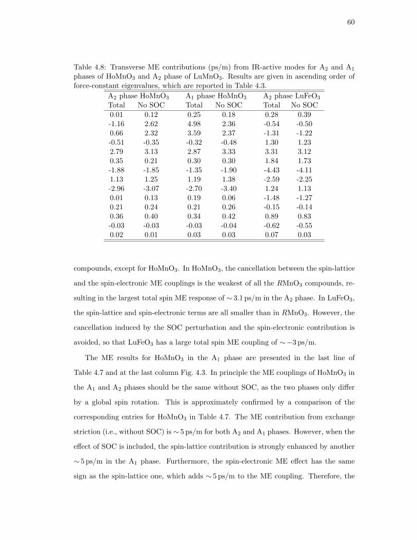
60

Table 4.8: Transverse ME contributions (ps/m) from IR-active modes for A2 and A1

phases of HoMnO3 and A2 phase of LuMnO3. Results are given in ascending order offorce-constant eigenvalues, which are reported in Table 4.3.

A2 phase HoMnO3 A1 phase HoMnO3 A2 phase LuFeO3

Total No SOC Total No SOC Total No SOC

0.01 0.12 0.25 0.18 0.28 0.39-1.16 2.62 4.98 2.36 -0.54 -0.500.66 2.32 3.59 2.37 -1.31 -1.22-0.51 -0.35 -0.32 -0.48 1.30 1.232.79 3.13 2.87 3.33 3.31 3.120.35 0.21 0.30 0.30 1.84 1.73-1.88 -1.85 -1.35 -1.90 -4.43 -4.111.13 1.25 1.19 1.38 -2.59 -2.25-2.96 -3.07 -2.70 -3.40 1.24 1.130.01 0.13 0.19 0.06 -1.48 -1.270.21 0.24 0.21 0.26 -0.15 -0.140.36 0.40 0.34 0.42 0.89 0.83-0.03 -0.03 -0.03 -0.04 -0.62 -0.550.02 0.01 0.03 0.03 0.07 0.03

compounds, except for HoMnO3. In HoMnO3, the cancellation between the spin-lattice

and the spin-electronic ME couplings is the weakest of all the RMnO3 compounds, re-

sulting in the largest total spin ME response of ∼ 3.1 ps/m in the A2 phase. In LuFeO3,

the spin-lattice and spin-electronic terms are all smaller than in RMnO3. However, the

cancellation induced by the SOC perturbation and the spin-electronic contribution is

avoided, so that LuFeO3 has a large total spin ME coupling of ∼−3 ps/m.

The ME results for HoMnO3 in the A1 phase are presented in the last line of

Table 4.7 and at the last column Fig. 4.3. In principle the ME couplings of HoMnO3 in

the A1 and A2 phases should be the same without SOC, as the two phases only differ

by a global spin rotation. This is approximately confirmed by a comparison of the

corresponding entries for HoMnO3 in Table 4.7. The ME contribution from exchange

striction (i.e., without SOC) is ∼ 5 ps/m for both A2 and A1 phases. However, when the

effect of SOC is included, the spin-lattice contribution is strongly enhanced by another

∼ 5 ps/m in the A1 phase. Furthermore, the spin-electronic ME effect has the same

sign as the spin-lattice one, which adds ∼ 5 ps/m to the ME coupling. Therefore, the

61

total spin ME coupling αyx reaches ∼ 15 ps/m, and is the largest in all of the RMnO3

and LuMnO3 materials we studied.


In summary, we have studied the spin-related magnetic charges and ME couplings for

HoMnO3, ErMnO3, YbMnO3, LuMnO3, and LuFeO3 using first-principles calculations.

It has been confirmed that the exchange striction acting on non-collinear spins induces

much larger magnetic charges than does SOC acting alone. Nevertheless, the effect of

SOC on ME couplings is surprisingly large, rivaling that of exchange striction in many

cases. This occurs because the exchange-striction contribution tends to be reduced by

cancellations between different IR-active modes, while the SOC contribution is mainly

associated with just a few low-frequency modes with large Mn displacements. It has also

been found that the RMnO3 materials have spin-electronic ME couplings comparable

to the spin-lattice ones. Among the RMnO3 and LuFeO3 materials we studied, the A1

phase of HoMnO3 is the most promising ME material, with the largest ME coupling

of ∼ 15 ps/m. Extrapolating the conclusions to other hexagonal RMnO3 and RFeO3

compounds that are not included in our calculations, we predict that the A2 phase is

more promising for the ferrites, while the A1 phase has a stronger ME coupling for the

manganites.

62

Chapter 5

Ferroelectricity in corundum derivatives

5.1 Introduction

Ferroelectricity requires a material to have a spontaneous electric polarization that can

be reversed by an external electric field. The search for new ferroelectric (FE) materials

holds promise for broadening our understanding of FE mechanisms and extending the

range of applications of FE materials.

The most intensively studied family of FE oxides is that of the perovskite oxides

[101, 102] such as BaTiO3. Perovskite oxides have the chemical formula ABO3 with the

A cation much larger than the B cation. The structure of a cubic perovskite is shown in

Fig. 5.1(a). The B cation has a 6-fold oxygen coordination which forms a BO6 oxygen

octahedron, and the perovskite structure is made up of these corner sharing octahedra.

The A cation occupies the hole of BO6 octahedra and has a 12-fold oxygen coordination.

If ions are stacked ideally in the cubic structure, the radius of A cation (rA), B cation

(rB) and O anion (rO) satisfy τ = (rA + rO)/√

2(rB + rO) = 1, and the ratio τ is called

the “Goldschmidt’s Tolerance Factor” [103]. The tolerance factor is an indicator for the

stability and distortion of perovskites, and if τ is not close to 1, the ideal cubic structure

is distorted to a lower symmetry. For example, in the case of a smaller τ , the A cation is

not large enough to fit into the interstices, thus BO6 octahedra rotations may develop

to reduce the A-O distance and optimize the coordination environment of the A cation

[104]. The FE distortion also lowers the symmetry and it is usually driven by B-site

off-centering which typically requires an empty d shell on the B cation. Therefore,

most FE perovskite oxieds does not have magnetism [105]. Recently, rocksalt-ordered

A2BB′O6 (and more complex AA′BB′O6 materials) double perovskites as sketched in

Fig. 5.1(b) have also attracted great interest [106, 107].

63

(a) (b)

A

B

B'

B

A

Figure 5.1: Structures of (a) a cubic perovskite ABO3 and (b) a double perovskiteA2BB

′O6.

The corundum derivatives ABO3 and A2BB′O6 make up a family of oxides that

can be derived from the corundum structure with cation ordering as shown in Fig. 5.2.

Some corundum derivatives are discovered in nature [108], and recently, more corun-

dum derivatives become available as metastable states through high-pressure synthesis

[109, 110, 111, 112, 113, 114, 115, 116, 117, 118, 119, 44]. Previous experimental and

theoretical studies suggest that most corundum derivatives are polar and exhibit large

polarization [120, 110, 121, 122, 114, 123], thus can potentially be new FE oxides similar

to the well-known FE LiNbO3(LNO) and LiTaO3.

Despite the similar chemical formula, corundum derivatives are different from per-

ovskites in many aspects. In corundum derivatives the A cation and B cation are com-

parable in size, so they have small tolerance factors (τ < 0.8) and large BO6 octahedra

rotations. The large rotation changes the local environment of A cation from 12-fold co-

ordination to 6-fold coordination which forms a distorted oxygen octahedron as shown

in Fig. 5.2. The rotation is so prominent that the high-symmetry reference structure for

corundum derivatives is rhombohedral instead of cubic, which is the high-temperature

paraelectric structure of perovskites. The polarization reversal mechanisms are also

distinct. In corundum derivatives, the polarization reversal is driven by the small A

or B cations migrating between oxygen octahedra [124, 125], so that d 0 configuration

64

is not required. This is in contrast to the off-centering displacement of d 0 B cations

in the oxygen octahedra in most perovskites. Therefore, corundum derivatives are also

good candidates for multiferroics and magnetoelectric effect [121].

Huge numbers of potential combinations of A, B and B′ cations in the ABO3 and

A2BB′O6 corundum-derivative family opens the possibility to achieve ferroelectricity,

multiferroicity and even more desirable properties. In this chapter, we focus on the

the polarization switching process of corundum derivatives, which is the crucial feature

that distinguishes FEs from polar materials. we use first-principles density functional

methods to systematically study polar structures and coherent FE reversal paths for a

variety of corundum derivatives. we first categorize corundum derivatives into four types

and show that only two of these allow for the possibility of FE reversal. Then a sys-

tematic method to analyze the coherent FE barrier and energy profile using structural

constraints are proposed and the method is applied to several corundum derivatives.

Furthermore, we identify several empirical measures that can provide a rule of thumb

for estimating the energy barriers. Finally, the possibilities of including magnetism and

hyperferroelectricity in corundum derivatives are discussed. These results lead us to

the prediction of several potentially new FEs.

5.2 Preliminary

5.2.1 Structure

Corundum derivatives ABO3 and A2BB′O6 can be derived from the corundum struc-

ture X2O3 with cation ordering as shown in Fig. 5.2. In the 10-atom rhombohedral unit

cell, the cations are spaced along the three-fold rotation axis and each one is surrounded

by a distorted oxygen octahedron. Two thirds of the oxygen octahedra are filled with

cations, while one third of them are cation-vacant.

Based on the combinations and arrangements of cations, corundum derivatives can

be classified into four types with notations as follows. An oxygen octahedron with an

A or B cation inside is written as “A” or “B”, and if an oxygen octahedron is cation-

vacant, the octahedron is denoted by “−”. This notation is then used to represent

65

α

β

γ

δ

Oxygen

ξ1

ξ2

Figure 5.2: Structure of corundum derivatives. The unit cell in the rhombohedralsetting is shown at the left; an enlarged hexagonal-setting view is shown at right. Thecations α, β, γ, and δ are are all identical in the X2O3 corundum structure. Forthe LNO-type ABO3, β = δ = A, α = γ = B; for the ilmenite ABO3, β = γ = A,α = δ = B; for the ordered-LNO A2BB

′O6, β = δ = A, γ = B, α = B′; for the ordered-ilmenite A2BB

′O6, β = γ = A, δ = B, α = B′. At left, ξ1 (or ξ2) is the distance betweenβ (or δ) and the oxygen plane that it penetrates during the polarization reversal.

the column of six face-sharing oxygen octahedra in the unit cell for each of the four

different types of corundum derivatives. Thus, the LNO-type ABO3 is AB−AB−,

the ilmenite ABO3 is AB−BA−, the ordered-LNO A2BB′O6 is AB−AB′−, and the

ordered-ilmenite A2BB′O6 is AB−B′A−. Other combinations, such as AA−BB−, are

connected to the four existing types as explained in the next section.

5.2.2 Coherent ferroelectric reversal

Experimentally, the FE polarization reversal process is a complicated one that typically

proceeds by nucleation and motion of domain walls, involving both intrinsic atomic mo-

tion and extrinsic pinning by defects. In this chapter, we focus only on the coherent FE

domain reversal, in which every unit cell undergoes the polarization reversal simulta-

neously. This coherent reversal process is clearly oversimplified and the barrier energy

of the coherent path is not equivalent to the coercive electric field in the FE hystere-

sis measurement. However, previous studies of perovskite oxides have shown that the

66

Table 5.1: Corundum-derived structures before and after polarization reversal.

Before After

LNO-type AB−AB− −BA−BAIlmenite AB−BA− −BB−AAOrdered-LNO AB−AB′− −BA−B′AOrdered ilmenite AB−B′A− −BB′−AA

coherent barrier provides a figure of merit that is often a useful indicator of the real

barrier to polarization reversal. For example, the well-known FE perovskite PbTiO3

has a coherent barrier around 0.2 eV per five-atom cell [101], hence perovskite oxides

with coherent barriers lower than this is considered likely to be FE.

The atomic origin of ferroelectricity in LiNbO3 is well-understood [124, 125]. In

LiNbO3 the polarization reversal is driven by an infrared (IR)-active mode that is as-

sociated with the motion of Li cations along the rhombohedral axis. In the reversal

process, each Li cation penetrates through an oxygen plane and migrates into an adja-

cent unoccupied oxygen octahedron. In our notation, the polarization reversal process

interchanges Li with −, so that the polar structure changes from LiNb−LiNb− to its

inversion image −NbLi−NbLi.

For all types of polar corundum derivatives, we assume that their polarization re-

versal mechanisms are similar to that of LiNbO3, i.e., that the reversal process inter-

changes A or B with −. The structures before and after this process are listed in

Table 5.1. Under such an operation, the LNO-type structure is transformed into its

own inversion-reversed image, which is a typical FE behavior. The same is true for the

ordered-LNO structure. By contrast, the ilmenite-type AB−BA− is transformed into

BB−AA−, and the ordered-ilmenite AB−B′A− into BB′−AA−. These structures are

not inversion-equivalent to the starting structures. Moreover, they exhibit face-sharing

A-containing octahedra, making them relatively unfavorable energetically. Addition-

ally, both the ilmenite structure and its switched partner are centrosymmetric. For

these reasons, ilmenite and ordered-ilmenite structures are excluded from our further

consideration as FE candidates.

67

5.2.3 Energy profile calculation

For the LNO-type and the ordered-LNO FE candidates, we firstly analyze the symmetry

of the reversal path. The ground state symmetry is R3c for LNO-type materials, and

R3 for ordered-LNO ones, but the symmetry of the reversal path is not straightforward.

For the coherent reversal, we assume that the three-fold rotation is always preserved,

so that the symmetry of the path can only be R3c or R3 for the LNO-type case, and R3

for the ordered-LNO case. If the structure acquires an inversion center at the midpoint

of the path when the polarization is zero (R3c or R3 for the two cases respectively),

the energy profile would be symmetric. If the inversion symmetry at the midpoint is

broken, as for example by magnetic orders, the energy profile would be asymmetric.

Different methods are adopted to calculate the energy profile of the FE reversal

based on the symmetry of the reversal path. In the case when the inversion symmetry

is present at the midpoint structure, the polarization reversal can be analyzed in terms

of an unstable IR-active phonon mode at the high-symmetry midpoint. In general,

even if the midpoint is not in a high-symmetry reference structure, the motion of the

small A cations is responsible for the polarization reversal. Therefore, we define ξ1 (ξ2)

to be the distance between the first (second) A cation and the oxygen plane that it

penetrates as this A cation moves along its path, as illustrated in Fig. 5.2. Then ξ1 + ξ2

is adopted as a “reaction coordinate” to describe the reversal. Finally, we use either the

unstable IR-active mode at the midpoint (for the high-symmetry case) or ξ = ξ1 + ξ2

(otherwise) as a structural constraint, and relax all other internal structural degrees of

freedom while stepping through a sequence of values of this constraint. This gives the

energy profile along the path, from which the energy barrier is obtained by inspection.



plemented in VASP [56]. The exchange-correlation functional that we use is PBEsol,

a revised Perdew-Burke-Ernzerhof generalized-gradient approximation that improves

68

equilibrium properties of densely-packed solids [51]. The ionic core environment is sim-

ulated by projector augmented-wave pseudopotentials (PAW) [61]. For transition metal

elements Mn and Fe, a Hubbard U = 4.2 eV is used on the 3d orbitals [53, 118]. For the

Os 5d orbital, a Hubbard U = 1.4 eV is used [123]. The magnetic moments are collinear

and spin-orbit coupling is neglected. The cutoff energy for all calculations is 550 eV.

The energy error threshold varied slightly in different calculations, but an accuracy be-

tween 1.0×10−5 and 1.0×10−7 eV is achieved in all calculations. The forces are reduced

below 0.001 eV/A for calculations of structural relaxation. A 6×6×6 Monkhorst-Pack

k-mesh is used in calculations. Linear-response methods are used to calculate the Γ-

point force-constant matrices. The spontaneous polarization is calculated using the

Berry phase formalism [34].


In this section, we apply the method introduced in previous sections to fully analyze

the coherent FE reversal path of the LNO-type corundum derivatives LiNbO3, LiTaO3,

ZnSnO3, FeTiO3, and MnTiO3, and the ordered-LNO corundum derivatives Li2ZrTeO6,

Li2HfTeO6, Mn2FeWO6, Mn3WO6 and Zn2FeOsO6. Among these materials, LiNbO3

and LiTaO3 are well-known ferroelectrics [108], so they are used as references for com-

parison. The high-pressure synthesized ZnSnO3 thin film [120] and FeTiO3 polycrystal

[110] have also been experimentally confirmed to be FE, while experimental results

for bulk crystals are absent. Similar to FeTiO3, MnTiO3 has also been predicted to

be FE from theoretical calculations [121], but the experimental evidence is lacking.

Ordered-LNO Li2ZrTeO6 and Li2HfTeO6 are stabilized at 700 [115] without detailed

investigation of FE properties. Mn2FeWO6 [44] and Mn3WO6 [126] are stabilized in

high pressure, but FE properties are still under experimental investigation. Zn2FeOsO6

is predicted to be FE from a previous theoretical calculation [123], but the compound

has not been synthesized yet.

69

Table 5.2: Rhombohedral structural parameters of LNO-type ABO3 corundum deriva-tives LiNbO3, LiTaO3, ZnSnO3, FeTiO3 and MnTiO3 from our first-principles calcu-lations and experiments [111, 127, 128, 129, 130]. The Wyckoff positions are 2a for Aand B cations, and 6c for oxygen anions (note that Ax= Ay= Az and Bx= By= Bz).The origin is defined by setting the Wyckoff position Bx to zero.

LiNbO3 LiTaO3 ZnSnO3 FeTiO3 MnTiO3

Calc. Exp. Calc. Exp. Calc. Exp. Cal. Exp. Calc. Exp.Lattice constants

a (A) 5.486 5.494 5.476 5.473 5.584 5.569 5.434 5.458 5.481 5.455α () 56.0 55.9 56.2 56.2 56.5 56.4 56.5 56.0 56.6 56.8

Wyckoff positionsAx 0.282 0.280 0.284 0.291 0.283 0.286 0.290 0.287 0.279 0.276Bx 0.000 0.000 0.000 0.000 0.000 0.000 0.000 0.000 0.000 0.000Ox 0.360 0.359 0.365 0.368 0.392 0.381 0.364 0.364 0.348 0.345Oy 0.719 0.720 0.726 0.732 0.709 0.721 0.721 0.720 0.721 0.731Oz 0.112 0.111 0.119 0.124 0.104 0.111 0.104 0.109 0.120 0.128

Table 5.3: Rhombohedral structure parameters of ordered-LNO A2BB′O6corundum

derivatives Li2ZrTeO6, Li2HfTeO6, Mn2FeWO6, Mn3WO6 and Zn2FeOsO6 from ourfirst-principles calculations and experiments [115, 44]. Wyckoff positions are 1a for A1,A2, B and B′ cations, and 3b for O1 and O2 anions. The origin is defined by setting theWyckoff position B′x to zero. For ordered-LNO Li2HfTeO6 and Zn2FeOsO6, no exper-imental results are available. Magnetic orders used in the calculation for Mn2FeWO6,Mn3WO6, and Zn2FeOsO6 are also indicated by “Mag”.

Li2ZrTeO6 Li2HfTeO6 Mn2FeWO6 Mn3WO6 Zn2FeOsO6

Calc. Exp. Calc. Calc. Exp. Calc. Exp. Calc.Mag — — — udu NA udu uud NA FiM

Lattice constantsa (A) 5.526 5.497 5.480 5.531 5.562 5.607 5.613 5.605 5.410α () 56.1 56.1 56.3 57.3 56.9 56.7 56.6 56.7 56.7

Wyckoff positionsA1x 0.291 0.298 0.289 0.286 0.278 0.287 0.283 0.283 0.284A2x 0.781 0.768 0.781 0.787 0.785 0.790 0.779 0.788 0.783Bx 0.504 0.507 0.504 0.506 0.493 0.508 0.493 0.510 0.504B′x 0.000 0.000 0.000 0.000 0.000 0.000 0.000 0.000 0.000O1x 0.366 0.390 0.366 0.356 0.347 0.356 0.384 0.351 0.376O1y 0.745 0.729 0.743 0.744 0.745 0.742 0.693 0.744 0.732O1z 0.111 0.133 0.115 0.109 0.102 0.102 0.124 0.104 0.114O2x 0.628 0.621 0.629 0.632 0.631 0.631 0.595 0.631 0.619O2y 0.219 0.235 0.222 0.207 0.197 0.199 0.234 0.190 0.223O2z 0.895 0.893 0.889 0.884 0.885 0.893 0.848 0.901 0.885

70

Table 5.4: Oxidation states of the LNO-type ABO3 and the ordered-LNO A2BB′O6

corundum derivatives. The oxidation state of O ion is −2 in all materials.

LNO-type A B Ordered LNO A B B′

LiNbO3 +1 +5 Li2ZrTeO6 +1 +4 +6LiTaO3 +1 +5 Li2HfTeO6 +1 +4 +6ZnSnO3 +2 +4 Mn2FeWO6 +2 +2 +6FeTiO3 +2 +4 Mn3WO6 +2 +2 +6MnTiO3 +2 +4 Zn2FeOsO6 +2 +3 +5

5.4.1 Ground state structure and magnetic order

The FE properties are sensitive to atomic displacements and strain, so it is essential

to start calculations with accurate structural parameters. The lattice constants and

Wyckoff positions obtained from our calculations are summarized in Tables 5.2 and

5.3 with experimental results provided for reference and the calculated structural pa-

rameters are very close to the experimental results. The oxidation states, obtained by

rounding the integrated charge around each cation, are also displayed in Table 5.4 and

are consistent with experimental observations.

The on-site spin moments are investigated for FeTiO3, MnTiO3, Mn2FeWO6, Mn3WO6,

and Zn2FeOsO6 by integrating the spin density inside the PAW sphere. DFT+U calcu-

lations predict that the magnetic moment is about 3.7µB on each Fe2+, 4.6µB on each

Mn2+, and 4.2µB on Fe3+. These results are in agreement with the high-spin d6 state

of Fe2+ and the high-spin d5 configuration of Fe3+ and Mn2+. The magnetic moment

on Os5+ is 2.1µB from our calculation, which is consistent with the high-spin d3 state

after taking into account the screening of the Os moment arising from the hybridization

between Os 5d and O 2p orbitals.

The energy of different magnetic orders that preserve the periodicity of the rhom-

bohedral unit cell is also studied. Calculation results suggest that the ground-state

magnetic order is antiferromagnetic (AFM) for FeTiO3 and MnTiO3 and ferrimagnetic

(FiM) for Zn2FeOsO6. To investigate magnetic structures of Mn2FeWO6 and Mn3WO6,

four different types of unit cell are considered in the calculation. We adopt a notation

like “udu” to describe the possible spin structure on the three cations excepting W.

71

Table 5.5: Magnetic energy of different magnetic states relative to the lowest-energystate in Mn2FeWO6 and Mn3WO6, in units of meV per unit cell.

Energyuuu uud udd udu

Mn2FeWO6 90.2 32.1 39.5 0.0Mn3WO6 101.8 1.0 19.2 0.0

Here “u” is spin-up, “d” is spin-down, and the spins are given on cations A1, A2 and

B in that order, where A1 and A2 are face-sharing with B′ and B cations, respectively.

(Note that A1, A2 and B correspond to cations β, δ and γ, respectivley, in Fig. 5.2.)

The four possible states (not counting those that are trivially related by a global spin

reversal) are uuu, uud, udu, and udd. The energy of each fully-relaxed magnetic struc-

ture is listed in Table 5.5. Of those, the most stable state for both Mn2FeWO6 and

Mn3WO6 is udu. However, for Mn3WO6, the energy difference between the uud and

udu states is tiny, so both magnetic states are considered in the study of polarization

reversal.

The magnetic ground states of Mn2FeWO6 and Mn3WO6 can be understood by

analyzing the superexchange interactions between the spins of A1, A2 and B cations.

The magnetic moments are coupled through the oxygen octahedra, and there are three

independent coupling constants. The moments on A2 and B sites are coupled through

face-sharing and corner-sharing oxygen octahedra with strength JA2B; the A1 and B

moments are coupled through edge-sharing octahedra with strength JA1B; and the A1

and A2 moments are coupled through corner-sharing octahedra with strength JA1A2 .

Then the magnetic energy Emag can be written as

Emag = JA1BSA1 · SB + JA2BSA2 · SB + JA1A2SA1 · SA2 , (5.1)

where S represent the spin direction on each site. Substituting the energy of different

magnetic orders in Table 5.5 into Eq.(5.1), it is discovered that the coupling constants

are all positive. This result means that the three magnetic moments all favor AFM

coupling. However, it is impossible to make three collinear spins couple antiferromag-

netically, and this frustration implies that one pair must be ferromagnetically coupled.

72

Table 5.6: Relative spin direction between different magnetic ions in Mn2FeWO6 andMn3WO6. Here “FM” means ferromagnetic.

uuu uud udd udu

A1 and B FM AFM AFM FMA2 and B FM AFM FM AFMA1 and A2 FM FM AFM AFM

In Table 5.6, we list the relative spin orientations of the magnetic ions. Since

the face-sharing coupling JA2B is the strongest, it is not surprising that the A2 and

B moments couple antiferromagnetically; the competition between JA1B and JA1A2

then determines the magnetic ground state. In Mn3WO6, these two couplings are

comparable, so the energy difference between the uud and udu states is tiny. In the

case of Mn2FeWO6, the magnetic moment on the B cation is smaller, so the coupling

JA1B is weaker than JA1A2 . Therefore, the lowest-energy state is udu.

5.4.2 Symmetry of the reversal path

For the LNO-type materials, the simplest possible reversal path would be one in which

the two A cations move synchronously, so that ξ1 = ξ2 everywhere along the path. In

this case the symmetry along the path is R3c, except at the midpoint where there is an

inversion center and the symmetry becomes R3c. Another possibility is that the cations

move sequentially, one after the other, so that ξ1 6= ξ2 for at least part of the path. In

this case the symmetry is R3 except at the R3 midpoint. In order to find out which

scenario occurs, we calculate the energy of the midpoint structures with symmetry R3c

and R3, respectively; the results are shown in Table 5.7. For all LNO-type materials

in Table 5.7, the R3 midpoint structure is energetically favored, which implies that the

reversal occurs via the lower-symmetry R3→R3→R3 scenario, at least in the central

portion of the path. Considering the fact that the high-temperature paraelectric phase

of LiNbO3 has the symmetry R3c [124, 125], this striking result demonstrates that the

midpoint of FE reversal path in the LNO-type FE materials is not identified with the

paraelectric structure, but instead has lower symmetry.

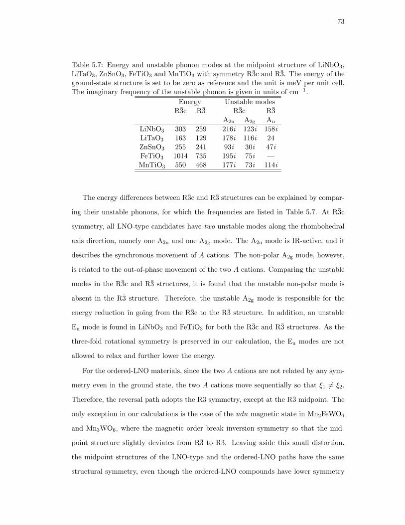
73

Table 5.7: Energy and unstable phonon modes at the midpoint structure of LiNbO3,LiTaO3, ZnSnO3, FeTiO3 and MnTiO3 with symmetry R3c and R3. The energy of theground-state structure is set to be zero as reference and the unit is meV per unit cell.The imaginary frequency of the unstable phonon is given in units of cm−1.

Energy Unstable modesR3c R3 R3c R3

A2u A2g Au

LiNbO3 303 259 216i 123i 158iLiTaO3 163 129 178i 116i 24ZnSnO3 255 241 93i 30i 47iFeTiO3 1014 735 195i 75i —MnTiO3 550 468 177i 73i 114i

The energy differences between R3c and R3 structures can be explained by compar-

ing their unstable phonons, for which the frequencies are listed in Table 5.7. At R3c

symmetry, all LNO-type candidates have two unstable modes along the rhombohedral

axis direction, namely one A2u and one A2g mode. The A2u mode is IR-active, and it

describes the synchronous movement of A cations. The non-polar A2g mode, however,

is related to the out-of-phase movement of the two A cations. Comparing the unstable

modes in the R3c and R3 structures, it is found that the unstable non-polar mode is

absent in the R3 structure. Therefore, the unstable A2g mode is responsible for the

energy reduction in going from the R3c to the R3 structure. In addition, an unstable

Eu mode is found in LiNbO3 and FeTiO3 for both the R3c and R3 structures. As the

three-fold rotational symmetry is preserved in our calculation, the Eu modes are not

allowed to relax and further lower the energy.

For the ordered-LNO materials, since the two A cations are not related by any sym-

metry even in the ground state, the two A cations move sequentially so that ξ1 6= ξ2.

Therefore, the reversal path adopts the R3 symmetry, except at the R3 midpoint. The

only exception in our calculations is the case of the udu magnetic state in Mn2FeWO6

and Mn3WO6, where the magnetic order break inversion symmetry so that the mid-

point structure slightly deviates from R3 to R3. Leaving aside this small distortion,

the midpoint structures of the LNO-type and the ordered-LNO paths have the same

structural symmetry, even though the ordered-LNO compounds have lower symmetry

74

Figure 5.3: Movements of A cations in LNO-type (red, here LiNbO3) and ordered-LNO(blue, here Mn2FeWO6) corundum derivatives along the polarization reversal path. ξ1

and ξ2 are the distances from A atoms to the oxygen planes that are penetrated duringthe polarization reversal, here rescaled to a range between −1 and 1. The symmetry atan arbitrary (ξ1, ξ2) point is R3; on the ξ1 = ξ2 and ξ1 =−ξ2 diagonals it is raised to R3cand R3, respectively; and at the origin (ξ1 = ξ2 = 0) it reaches R3c. Green diamondsdenote the midpoint structure in the parameter space. In the LNO-type case “path1”and “path2” (filled and open red square symbols) are equivalent and equally probable,while the ordered-LNO system deterministically follows “path1” (full blue line), whichbecomes “path2” (dashed blue) under a relabeling ξ1 ↔ ξ2.

in their ground state.

The sequence of movements of the A cations along the FE reversal path is illus-

trated in Fig 5.4, and described quantitatively using our computed results for LiNbO3

and Mn2FeWO6 as paradigmatic examples in Fig. 5.3. The “Before” and “After” struc-

tures in Fig. 5.4 correspond to the points at the top right and bottom left corners of

Fig. 5.3, respectively. For the LNO-type case, the ideal R3c “Midpoint” structure would

correspond to the origin on the plot, but the reversal path does not pass through this

point because of an unstable A2g mode along the ξ1 = −ξ2 direction. The “bubble” in

the center confirms the significant effect of the unstable A2g mode. The “Midpoint” in

75

Before Midpoint After

Figure 5.4: Structural evolution along the polarization reversal path of LNO-type andordered-LNO corundum derivatives. “Before” and “After” are the initial and finalstructures on the reversal path with symmetry R3c for the LNO-type and R3 for theordered-LNO corundum derivatives; “Midpoint” denotes the structure halfway betweenthese and exhibits R3 structural symmetry in both cases.

Fig. 5.4 is thus displaced from the origin along the line ξ1 =−ξ2. There is a sponta-

neous breaking of symmetry at the point where the structure departs from the ξ1 = ξ2

diagonal; at this point the system “randomly” makes a choice between two equivalent

paths, marked by filled and open red symbols in Fig. 5.3.

For the ordered-LNO materials the two A cations are inequivalent, and one of them

is already closer to the oxygen plane in the ground state. Let this be the one labeled by

ξ1. Therefore, it is energetically favorable for this particular A cation to migrate first

in the reversal path, which causes either the B or B′ cation to be sandwiched between

two A cations in the ‘Midpoint” structure as illustrated in Fig. 5.4. The system thus

deterministically follows the path indicated by the full blue line in Fig. 5.3, with the

configuration always staying on one side of the ξ1 = ξ2 diagonal. If we would reverse

the convention on the definition of ξ1 and ξ2, the system would be described by the

dashed blue path in Fig. 5.3.

76

-1 0 10

50

100

150

200

250

300 LiNbO3

LiTaO3

Mn2FeWO6

Zn2FeOsO6

Li2ZrTeO6

barr

ier e

nerg

y (m

eV)

relative constraint amplitude

Figure 5.5: Polarization reversal energy profile for LiNbO3, LiTaO3, Mn2FeWO6,Zn2FeOsO6, and Li2ZrTeO6.

5.4.3 Polarization reversal barrier

Using structural constraint methods, we compute the relaxed structures and energies

for a sequence of constrained values of reaction coordinate for each material of interest.

A selection of results for the energy along the path are presented in Fig. 5.5, and

quantitative results for the energy barrier Ebarrier and the spontaneous polarization PS

in the ground-state structure are reported in Table 5.8. For Mn3WO6 and Mn2FeWO6

with udu magnetic order, the FE reversal changes the magnetic state to duu, so that

the energy profile is no longer symmetric and the two minima become inequivalent. For

these two compounds, the value of the energy barrier in Table 5.8 is that of the highest

barrier along the transformation path. Among the computed energy barriers, those

for ZnSnO3, Li2ZrTeO6, Li2HfTeO6, Mn2FeWO6, Mn3WO6, and Zn2FeOsO6 are lower

than or comparable to those of the established FE materials LiNbO3 and LiTaO3.

The midpoint of ordered-LNO have two possible structures in which either B or

B′ cation is sandwiched by two A cations. Comparing energy of the two midpoint

structures ∆E= EB − EB′ listed in Table 5.9, it is found that the sandwiched cations

77

Table 5.8: Coherent polarization reversal barrier Ebarrier (meV) per unit cell and spon-taneous polarization PS (µC/cm2) for FE candidates.

LNO-type Ebarrier PS Ordered-LNO Ebarrier PS

LiNbO3 259 82 Li2ZrTeO6 57 33LiTaO3 129 57 Li2HfTeO6 61 32ZnSnO3 241 57 Mn2FeWO6 215 63FeTiO3 763 105 uud Mn3WO6 240 69MnTiO3 468 94 udu Mn3WO6 272 70

Zn2FeOsO6 92 52

are Zr for Li2ZrTeO6, Hf for Li2HfTeO6, W for Mn2FeWO6 and Mn3WO6, and Os for

Zn2FeOsO6. The results can also be directly predicted from their ground state. For the

ordered-LNO materials the two A cations are inequivalent, and one of them is already

closer to the oxygen plane in the ground state,. Therefore it is energetically favorable

for this particular A cation to migrate first in the reversal path, which causes either the

B or B′ cation to be sandwiched between two A cations in the midpoint structure. Let

me denote the distance between A1 (or A2) cation and the oxygen plane in the ground

state by ξ1S (or ξ2S). If ξ1S > ξ2S, the sandwiched cation is B; otherwise it is B′. The

above analysis is consistent with the calculated energy difference between the B and

B′ sandwiched midpoint structures, as shown in Table 5.9. In addition, it is found that

the energy difference between the two distinct midpoint structures is mainly due to the

difference of Madelung energies ∆EM = EMB − EM

B′ of the two structures in a simple

point-ion model, as shown in Table. 5.9.

We have analyzed the calculation results in an attempt to extract empirical rules

of thumb that may help point in the direction of more new materials with low reversal

barriers. Firstly, we have considered how the energy barriers are correlated with the

spontaneous polarizations. In a FE material the energy E is often approximated as a

double well of the form E(P ) = E0 − µP 2 + νP 4 with positive µ and ν. Minimizing

E(P ) within this model gives the spontaneous polarization as P 2S = µ/2ν and the energy

barrier Ebarrier = E(0)−E(PS)= µ2/4ν, which can also be written as Ebarrier = (µ/2)P 2S .

Thus, as long as µ can be taken as approximately constant, Ebarrier is proportional

to P 2S . Interestingly, it is found that the computed coherent barrier energies Ebarrier

78

Table 5.9: Midpoint structures of ordered-LNO candidates and the energy differencesbetween B and B′ sandwiched midpoint structures. The distances between A1 (or A2)cation and the oxygen planes in the ground state are characterized by ξ1S (or ξ2S). Theenergy difference between the B and B′ sandwiched midpoint structures is ∆E. TheMadelung energy difference between the B and B′ sandwiched midpoint structures is∆EM.

Ordered-LNO B B′ Sandwiched ξ1S (A) ξ2S (A) ∆EM (meV) ∆E (meV)

Li2ZrTeO6 Zr Te Zr 0.607 0.559 -186 -48Li2HfTeO6 Hf Te Hf 0.582 0.550 -94 -29Mn2FeWO6 Fe W W 0.623 0.707 2085 225uud Mn3WO6 Mn W W 0.635 0.799 1666 266udu Mn3WO6 Mn W W 0.642 0.790 1499 290Zn2FeOsO6 Fe Os Os 0.565 0.574 382 102

roughly follow this trend with µ/2 = 0.057 meVcm4/µC2 as shown in Fig. 5.6. Therefore,

the results suggest that FE corundum derivatives are more likely to be discovered in

materials having a relatively low spontaneous polarization.

Furthermore, we have investigated the correlation between the spontaneous polar-

izations and the geometric properties of the crystals. Our results suggest that for each

FE candidate, the polarization P along the reversal path is almost linearly related to

the reaction coordinate ξ. Expecting P (ξ) to be an odd function, we add a small cubic

part and fit it as P (ξ) = mξ + nξ3. The parameters m and n are different in each

material, and they are determined by several factors that are not included in the reac-

tion coordinate ξ, such as displacements of the B cations and valence states of the A

cations. Despite these differences between materials, it is found that the spontaneous

polarizations PS of corundum derivatives are correlated with the reaction coordinate

ξS = ξ1S + ξ2S in the spontaneously polarized ground state, as shown in Fig. 5.7. This

time a roughly linear fit clearly does not work. Again we try fitting PS(ξS) to an

odd third-order polynomial, and find that PS = mξS + nξ3S gives a reasonable fit with

m= 13.3 × 108 µC/cm3 and n= 19.0 × 1024 µC/cm5 as shown in the figure. As the

distance between A cations and oxygen planes can be experimentally determined, this

empirical rule can provide a rough estimation of the spontaneous polarization.

79

0 2000 4000 6000 8000 100000

100

200

300

400

500

600

700

800

udu Mn3WO6

uud Mn3WO6

LiTaO3Li2ZrTeO6

Mn2FeWO6

ZnSnO3

Zn2FeOsO6

Li2HfTeO6

LiNbO3

MnTiO3

Ebarrier

Linear fitting of Ebarrier with adjusted R2=0.955

barr

ier e

nerg

y (m

eV)

P2S (C2/cm4)

FeTiO3

Figure 5.6: Empirical proportionality between the coherent FE energy barrierand P 2

S . The red curve is the fitting polynomial Ebarrier = (µ/2)P 2S , with

µ/2 = 0.057 meVcm4/µC2.

0.0 0.2 0.4 0.6 0.8 1.0 1.2 1.4 1.6 1.8 2.00

20

40

60

80

100

120

PS (

C/c

m2 )

PS

Polynomial fitting of PS

with adjusted R2=0.970

S (A)

uud Mn3WO6

udu Mn3WO6

LiTaO3

Li2ZrTeO6

Mn2FeWO6

ZnSnO3Zn2FeOsO6

Li2HfTeO6

LiNbO3

MnTiO3

FeTiO3

Figure 5.7: Empirical correlation between the spontaneous polarization and the reactioncoordinate ξ in the ground state. The red curve is the fitting polynomial PS = mξS+nξ3

S

with m= 13.3× 108 µC/cm3 and n= 19.0× 1024 µC/cm5.

80

-1 0 10

100

200

300

400

500

600

700

800

c

b

Barrier Gap

Relative constraint amplitude

Bar

rier e

nerg

y (m

eV)

a0.0

0.5

1.0

1.5

Gap

(eV

)

Figure 5.8: Energy profile and bandgap at the polarization reversal path of FeTiO3.The band gap is 1.56 eV and 0.98 eV at points a and c, but FeTiO3 is conducting atpoint b.

5.4.4 Insulating vs conducting

FeTiO3 and Mn2FeWO6 do not stay insulating along the coherent reversal path. The

energy profile and bandgap of FeTiO3 along the path is shown in Fig. 5.8 as an illus-

tration. FeTiO3 has a finite gap at points a and c, but becomes conducting at point

b. In order to understand the orbital character around the Fermi energy, the projected

density of states (PDOS) of points a,b, and c are shown in Fig 5.9(a-c), respectively.

A detailed analysis of the occupied d orbitals along the path reveals the reason

for this metal-insulator transition. In the local octahedral environment of the ground

state, the d orbitals are split into triply degenerated t2g and doubly degenerated eg

orbitals. Under the threefold rotational symmetry, the t2g orbitals are further split into

a1g and doubly degenerate e′g irreps. The a1g state has orbital character dz2 with charge

lobes directed along the rhombohedral axis, and since these lie closer to the neighboring

cations, the energy of the a1g state is lowered. Therefore, the ground-state arrangement

of d orbitals in order of increasing energy is a1g followed by e′g and then eg. In FeTiO3

and Mn2FeWO6, Fe is in the 2+ valence state and has a d6 configuration. In the ground

81

-10

-5

0

5

10

EF=4.49 eV(c)

(b) PDOS Fe(d)

PDOS O(p)

PDOS Ti (d)

(a)EF=4.47 eV

-10

-5

0

5

10

Den

sity

of s

tate

s (a

.u.)

2 3 4 5 6 7 8

-10

-5

0

5

10

EF=5.72 eV

Energy (eV)

Figure 5.9: PDOS of FeTiO3 at point (a), (b), and (c) along the coherent reversal path.Position of Fermi energy are indicated by dashed black lines. The density of statesfrom two spin channels are represented by the positive branch and negative branch ofdensity of states, respectively. The unit a.u. means arbitrary unit.

(a) (b)

eg

t2ge'ga1g

eg

t2ga1ge'g

Figure 5.10: Sketch of energy levels of d orbital in the (a) insulating case and (b) theconducting case.

82

Figure 5.11: M-H relation (between -14 and 14 T) of Mn2FeWO6 at 2, 70, 120, and400 K, taken from Ref. [44].

state, five electrons fully occupy one spin channel and the remaining one occupies the

a1g orbital in the minority spin channel, as shown by the PDOS in Fig. 5.9(a) and the

energy level sketch in Fig. 5.10(a). However, during the polarization reversal process,

the Fe2+ ion temporarily moves away from its neighboring cations, and as a result, the

a1g orbital is no longer energetically favored. Instead, the minority electron occupies

the doubly degenerate e′g orbitals, leading to a metallic state, as shown in Fig. 5.9(b)

and Fig. 5.10(b). Since a metallic state along the polarization reversal path could short

out the applied bias, it may be that the switching of polarization is not possible in such

cases. Therefore, we propose that d3, d5, and d8 orbital configurations should be much

more likely to avoid this conducting problem, and are therefore more suitable targets

in the search for ferroelectrically switchable magnetic corundum derivatives.

5.4.5 More complicated magnetic structures

In previous sections, only magnetic orderings that preserve the periodicity of the rhom-

bohedral unit cell were considered, since our major focus is on the polarization reversal

mechanism. Under such an assumption, the ground state magnetic order of Mn2FeWO6

is FiM udu at T = 0 K with a net magnetization of ∼ 4µB. However, according to the

experimental M-H relation [44] shown in Fig. 5.11, the magnetic structure at 2 K does

not have a net magnetization at zero field, but exhibits an AFM double-hysteresis loop.

83

Table 5.10: Magnetic energies for AFM doubled-cell magnetic structures. ∆E1 is forenergies evaluated at the unrelaxed experimental structure, while ∆E2 applies to en-ergies calculated after relaxation of the internal coordinates. The energy is given withrespect to the udu magnetic order in the experimental cell with unit meV/f.u. .

Magnetic order udu uuu-ddd uud-ddu udu-dud udu-udd duu-udd

∆E1 0 22 8 14 11 23∆E2 -202 -197 -208 -204 -210 -192

In order to explain the observed low-temperature magnetic behavior, we consider

AFM doubled-cell magnetic structures containing two formula units (f.u.). In the

doubled-cell magnetic structure, one cell has a positive magnetization with a mag-

netic order uuu, uud, udu or duu, and the other cell has the opposite magnetization.

Therefore, only five possible doubled-cell magnetic orders do not exhibit net magne-

tization, and they are uuu-ddd, uud-ddu, udu-dud, udu-udd, and duu-udd. In these

notations, the letters before or after “-” are the magnetic orders in the first or second

cell. Among these magnetic orders, four of them are composed by two subcells with

magnetic orders that are related by time-reversal symmetry, and the only exception is

the magnetic order udu-udd.

The energy of the five doubled-cell magnetic structures are shown in Table 5.10.

With the unrelaxed experimental structure [44], the lowest-energy magnetic ordering

among the doubled-cell configurations is uud-ddu, i.e., the one obtained by a combina-

tion of uud and ddu primitive cells. After relaxation of the internal coordinates, how-

ever, the udu-udd magnetic structure becomes the most stable. The energy reduction

from lattice relaxation is largest for the udu-udd composite cell because the magnetic

order of the two subcells is not related by time-reversal symmetry, so that additional

zone-boundary phonon modes can relax and contribute to lowering the energy. The

udu-udd double cell is even lower in energy than the udu single-formula-unit structure,

by 8 meV/f.u. Therefore, the results suggest that the magnetic double-hysteresis loop

visible at low temperature in Fig. 5.11 might be understood as a series of transitions

from a dud FiM order at negative field to a udu-udd (or dud-duu) configuration at zero

field, then back to a udu FiM configuration at positive field.

84

Table 5.11:R3c R3

TO LO TO LO

LiNbO3 216i 109i 158i 150LiTaO3 178i 74i 24 143

We have only considered collinear magnetic structures here. However, our study of

the doubled-cell structures strongly suggests that there is a magnetic phase transition

at finite magnetic field, below which the magnetic order is AFM, in a magnetic unit

cell including at least two formula units, possibly with a more complex non-collinear

magnetic structure that has not been considered here. Above the critical magnetic field,

we expect the system to adopt the collinear udu FiM structure, with a single-formula-

unit magnetic cell.

5.4.6 Hyperferroelectric?

Hyperferroelectrics are a class of proper FEs that polarize even at D = 0 (vanishing

electric displacement field) boundary conditions when the depolarization field is un-

screened [11]. This condition is equivalent to the instability of a longitudinal optic

(LO) mode, in addition to that of a transverse optic (TO) mode which is the charac-

teristic of proper FEs. In a previous study [131], it was theoretically proposed that

LiNbO3 and LiTaO3 are hyperferroelectric, because there is an unstable LO mode at

the paraelectric R3c structure. However, our study of the polarization reversal path

suggests that the FE polarization reversal does not pass through the structure with

R3c symmetry, and instead the high-symmetry midpoint structure has the symmetry

R3. Therefore, it would be more relevant to study the LO mode instability at the R3

midpoint structure.

Here we use Eq. 1.3 introduced in Chapter 1 and frequencies of the TO modes

shown in Table 5.7 to calculate the frequencies of the LO modes, and the results for

the unstable polar modes are summarized in Tabel 5.11. In the R3c structure, both

the TO modes and the LO modes are unstable, consistent with previously reported

85

frequencies [125, 131]. As a result, in the PR3c structure with D = 0 condition, the

LO mode displacement can lower the energy, and bring the structure to a stable state

at R3c symmetry with a finite polarization. Here we use the notation PR3c to denote

the polar state. However, in the R3 structure, the TO modes get less unstable and the

LO modes are stabilized. Therefore at D = 0 boundary condition, the non-polar R3

structure is also a stable state and we call it NPR3.

Although we have shown that there is no unstable LO mode in the R3 structure

in LiNbO3 and LiTaO3, we cannot conclude that they are not hyperferroelectric yet.

After all, if the NPR3 state is only a metastable state, and the energy of the PR3c state

is lower than that of NPR3, a finite polarization can still exists at D = 0. To answer

this question, calculation in the D = 0 boundary condition is required to explore the

PR3c state, which is not the calculation we have done at E = 0. Therefore, this question

is left for future investigations.


In this chapter, we have proposed a method to study the coherent FE reversal path of

the corundum derivative family. By analyzing the structures, it is shown that only the

LNO-type and the ordered-LNO corundum derivatives can be FE in the usual sense. we

have calculated the energy profiles of the reversal paths using first-principles density-

functional methods. Our calculations reveal that the symmetry of the FE barrier struc-

ture is lower than that of the paraelectric phase. According to the calculated energy

barrier, ZnSnO3, Li2ZrTeO6, Li2HfTeO6, Mn3WO6, and Zn2FeOsO6 are predicted to

be possible new FEs. In addition, we have found empirically that the energy barrier is

roughly proportional to the the square of the spontaneous polarization, and that the

spontaneous polarization is strongly correlated with the reaction coordinate ξ in the

ground state. Furthermore, we have also argued that magnetic corundum derivatives

are unlikely to be suitable for FE switching unless the magnetic ion is d3, d5 or d8, since

metallic configurations otherwise tend to appear along the FE reversal path. At last, by

considering the possible doubled-cell AFM magnetic structures in Mn2FeWO6, we have

purposed a possible explanation for the observed double-hysteresis loop in experiments.

86

Meanwhile, there are still many open questions that remain to be answered. Firstly,

the polarization reversal path is only studied for the coherent reversal, which is not

the actual physical process observed in experiments. The polarization reversal occurs

through the motion of FE domain walls, which only have the thickness of a few unit

cells for many FEs. Therefore, the reversal energy barrier and electronic structure at

the domain walls might be very different from the bulk and the coherent reversal, and

this is the subject of the next chapter. Secondly, we have only briefly discussed the

hyperferroelectricity in LiNbO3 and LiTaO3, and more investigations in the D = 0

boundary conditions are needed to answer this question. Lastly, the predictions of

magnetic orders are tricky if the magnetic symmetry is unknown. In the study of the

coherent polarization reversal, we have only considered the simplest possible magnetic

orderings which are consistent with the rhombohedral unit cell. However, it is found

that in Mn2FeWO6, a double-cell magnetic order is more stable, and we would not be

surprised if the actual magnetic structure is even more complicated with non-collinear

spins in a much larger magnetic cell.

87

Chapter 6

Ferroelectric and magnetoelectric domain walls in

corundum derivatives

6.1 Introduction

In Chapter 5, we discussed the coherent ferroelectric (FE) reversal process in corundum

derivatives. However, the hysteresis behavior of FE reversal is caused by the nucleation,

expansion or shrinkage of domains through the motion of domain walls in an applied

electric field. FE domains are regions of different polarization orientations that may

coexist in a FE crystal. The interface between two domains are referred to as a domain

wall (DW). The experimental images of FE domains and DWs of LiNbO3 [132] and

YMnO3 [133] are shown in Fig. 6.1 as an illustration. An applied electric field would

favor the domains with polarization paralleled to the field, so these domains would ex-

pand to gain electric energy while the opposite domains would shrink, which is achieved

through the motion of domain walls. Meanwhile, defects can be attracted to the DW

and can pin the DW motion [134].

DWs can be seen as topological defects which have different geometric and electronic

structures compared to the bulk, so DWs may exhibit rich physics that is not present

in the bulk. For instance, in the FE-antiferromagnetic insulating BiFeO3, experiments

have shown that the DWs behave as conductive channels in the otherwise insulating

background [135]. Meanwhile, the same DWs are suggested to exhibit photovoltaic

properties as well [136]. Furthermore, it is recently observed that charged FE DWs,

which are energetically unfavorable in general, are abundant in hybrid improper FEs

(Ca,Sr)3Ti2O7 [137]. Moreover, in hexagonal manganite RMnO3 (R = Sc, Y, In,

and Ho-Lu), the FE DWs form topologically protected vortices [133], and alternating

magnetic moments are found at the FE DW around the vortex core [138]. In addition,

88

(a) (b)

Figure 6.1: FE domains and domain walls observed in (a) LiNbO3, taken from Ref. [132]and (b) YMnO3, taken from Ref. [133]

the FE DWs are also observed interlocking with chiral DWs in Ni3TeO6[139].

In the newly proposed FE corundum derivatives, the properties of FE DWs and the

role of DWs in polarization reversal are not clear. Firstly, many corundum derivatives

are in the form of powder samples because of the high-pressure syntheses, so that

the growth of single crystals and the observations of domains and DWs are an on-

going problem. Secondly, corundum derivatives may exhibit magnetic orders in the

ground state, making them multiferroics. Even if the origin of the polarization and

magnetization are different in the bulk, the distinct structure at the domain wall may

enhance the coupling between the polarization and magnetization. Thirdly, the ordered-

LNO exhibits a chiral structure, so there might be an interplay between chiral domains

and FE domains. Finally, as the DW structure is very different from the bulk, it would

be interesting to investigate how the DW structure would influence the reversal barrier.

In this chapter, we use first-principles methods to study the formation and motion

of FE DWs at the atomic scale in order to characterize the properties of DWs and their

role in the FE reversal process. The FE candidates that we consider are LiNbO3(LNO),

LiTaO3, ZnSnO3, FeTiO3, MnTiO3, Li2ZrTeO6, Li2HfTeO6, and Mn3WO6. Our study

of the 180 charge-neutral DWs predicts the orientation and shape of DWs in corundum

derivatives. Moreover, the DW formation energy also suggests that in ferrimagnetic

Mn3WO6, the FE DWs are simultaneously magnetic DWs, and when the polarization

89

at the DW is reversed by an electric field, so is the magnetization. Therefore, this study

demonstrates a strong magnetoelectric coupling at the DW of corundum derivatives.

Finally, we point out that the DW-mediated reversal barrier is strongly correlated with

the local bonding environment of A cations.



plemented in VASP [56] with PBEsol [51] as the exchange-correlation functional. The

ionic core environment is simulated by projector augmented-wave (PAW) pseudopoten-

tials [61]. We use a Hubbard U = 4.2 eV on the 3d orbitals of Mn and Fe [53]. The

magnetic moments are collinear and spin-orbit coupling is neglected. The cutoff energy

for all calculations is 550 eV. The energy error threshold varies slightly in different cal-

culations, but an accuracy between 1.0×10−5 and 1.0×10−7 eV is achieved. The forces

are reduced below 0.01 eV/Angstrom in the DW structural relaxations. A 2 × 6 × 2

Monkhorst-Pack k-mesh is used in X-wall calculations, and a 6×6×1 k-mesh is used in

the Y-wall calculations.


6.3.1 Construction of domain walls

The general structure of corundum derivatives ABO3 and A2BB′O6 were introduced

in Chapter 5, and here we only focus on the LNO-type and ordered-LNO structure

which are compatible with ferroelectricity at the rhombohedral [111] direction. In

Fig. 6.2, both the rhombohedral unit cell and views from different hexagonal directions

are illustrated. Each cation is in a distorted oxygen octahedron and one third of the

oxygen octahedra are cation-vacant, which is denoted by “−” as defined in Chapter 5.

The FE reversal is driven by migration of A cations from their own oxygen octahedron

to the cation-vacant octahedron above or beneath them [124, 125] and the reversal

path can be qualitatively described by two variables ξ1 and ξ2 defined as the vertical

distances between each A cation and the oxygen plane that it penetrates during the

90

ξ2

ξ1

(a)

A B B' Oxygen

(c)

[0001]

[1100]

(b)

[0110]-

[2110]- -

-

C1C2

C3

C1

C1C3

C3

Figure 6.2: Structure of LNO-type corundum derivative ABO3 when B′ = B, andordered-LNO corundum derivative A2BB

′O6. (a) Side view of the rhombohedral unitcell. ξ1 (or ξ2) is the vertical distance between an A cation and the oxygen plane thatit penetrates during the polarization reversal. (b) Top view of the AB layer and (c)side view in the enlarged hexagonal-setting cell. The enlarged hexagonal cell consistsof three columns of octahedra C1, C2, and C3.

polarization reversal. The definitions of ξ1 and ξ2 are also shown in Fig. 6.2(a).

In order to study the properties of DWs, we construct a supercell with a polarization-

up domain and a polarization-down domain that are related by the inversion symmetry,

and the boundary between them is a FE DW [140]. Because of periodic boundary

conditions, there are always two DWs in the supercell, a left-up-right-down DW⇑⇓

and a left-down-right-up DW⇓⇑, where ⇑ and ⇓ represent up and down polarization

directions. In corundum derivatives, the R3c symmetry of the LNO-type structure

ensures that the DW⇑⇓ and DW⇓⇑ are equivalent, but in the ordered-LNO structure

with R3 symmetry, the two DWs are inequivalent. However, as DW⇑⇓ and DW⇓⇑

coexist in calculations with periodic boundary conditions, we report the averaged DW

91

R↑ L↓

Inversion(b)(a)

L↑ R↑

Mirror

(c)

R↑ L↓ R↑ L↓

DW↑↓ DW↓↑

Figure 6.3: Illustration of domains and DWs in chiral polar object. Left and righthands represent left (L) and right (R) chirality, and the direction in which the fingerspoint (⇑ or ⇓) represents the polarization direction. (a) Left and right chirality arerelated by a mirror symmetry. (b) Upward right hand (R⇑) and downward left hand(L⇓) are related by the inversion symmetry. (c) FE domains and DWs formed by (R⇑)domains and (L⇓) domains. The DW between adjacent thumbs represents DW⇑⇓ andthe DW between adjacent little fingers represents DW⇓⇑.

formation energy between DW⇑⇓ and DW⇓⇑ for ordered-LNO materials.

The intrinsic difference between DW⇑⇓ and DW⇓⇑ in ordered-LNO are attributed

to the chiral nature of the structure. A structure is chiral if it is distinguishable from

its mirror image. The symmetry of ordered-LNO is R3 which does not contain any

mirror symmetry, so it has a chiral structure. In contrast, the LNO-type structure is

not chiral because its symmetry is R3c. The term chirality is derived from the Greek

word for hand; left hand has left chirality (L) while right hand has right chirality (R).

In Fig. 6.3, hands are used as an illustration of FE domains to explain why DW⇑⇓ and

DW⇓⇑ are inequivalent. The direction that the fingers are pointing towards represents

the polarization direction, and the left or right hand represents the chirality L or R.

The spatial inversion operation changes (x, y, z) to (−x,−y,−z), so the upward right

hand (R⇑) becomes the downward left hand (L⇓) under inversion, through which both

92

polarization and chirality are flipped, as shown in Fig. 6.3(b). The domains and DWs

formed by upward right hands and downward left hands are shown in Fig. 6.3(c).

It is apparent that the FE DW is also a chiral DW in chiral polar materials, and

this interlocking effect between polarization and chirality at the DW is observed in

chiral pyroelectric Ni3TeO6[139]. It is also clear that there are two kinds of interfaces

between hands, one between thumbs and the other one between little fingers, and these

correspond to the DW⇑⇓ and DW⇓⇑.

Chirality can qualitatively explain or predict the shape of domains in corundum

derivatives. In LiNbO3 and other LNO-type materials with symmetry R3c, because

DW⇑⇓ and DW⇓⇑ are identical, according to the Wulff construction [141], domains of

LNO-type should form regular hexagons. In contrast, in order-LNO, domains should

form equiangular but not equilateral hexagons, or even triangles. In fact, the regular-

hexagon-shape domains are observed in LiNbO3 [132] as shown in Fig. 6(a), while

triangle shape domains are found in Ni3TeO6 with ordered-LNO structure [139].

To arrive at our domain wall configurations, we assume that the B/B′ and O sub-

lattices are preserved throughout the supercell, so that the DW only results from the

interchange of A and “−” sublattices (that is, migration of A cations into vacancies) on

one side of the DW. This is motivated by the greater mobility of the A cation species.

In addition, only the 180 charge-neutral DW is considered, in which the polarization

direction is parallel to the DW plane but antiparallel between domains.

6.3.2 Orientation of domain walls

Since corundum derivatives have three-fold symmetry, there are two types of 180 DWs

depending on the orientation of the DW plane. The DW in the x-z plane is called the

X-wall and the one in the y-z plane is called the Y-wall. The top view and the side view

of the X-wall and Y-wall are shown in Fig. 6.4 in comparison with the bulk structure

in Fig. 6.2(b-c). In the layer shown in Fig. 6.4(a), octahedra containing A cations

are densely packed at the X-wall. However, there are also layers where the octahedra

at the X-wall are all cation-vacant. In short, the X-wall consists of alternating dense

and sparse octahedra layers. In comparison, the A and − sublattices are more evenly

93

21

43

65

98

7

111012

(a)

(b)

(c)

2 64 8 10 12

(d)

(e)

(f)

12

54

36 8

7

81 2 543 76

C1C2

C3

C1

C1C3

C3

Figure 6.4: Structures of X-wall in the 6+6 supercell and Y-wall in the 4+4 supercell.(a)(d) Top views of the X-wall and Y-wall. The number in each octahedron is the unitcell label. The X-wall is in the x-z or (0110) plane and is located between the 6th andthe 7th unit cell, shown by the dashed line. The Y-wall is in the y-z or (2110) planeand is located between the 4th and the 5th unit cell. (b)(e) Side views of the X-walland Y-wall. Odd-number cells are behind even-number cells in the X-wall. (c)(f) Theξ1 +ξ2 displacement profile of X-wall and Y-wall. (d) C1, C2, and C3 are three differentcolumns of octahedra in the left-side domain. C1 and C3 are columns of octahedra inthe right-side domain. The column C1 becomes C1 after the polarization reversal.

94

Table 6.1: Formation energy of X-wall and Y-wall. For the ordered-LNO structure, theformation energy is averaged between the DW⇑⇓ and DW⇓⇑. The unit is mJ/m2.

LNO-type Magnetic order X Y Ordered-LNO Magnetic order X Y

LiTaO3 71 63 Li2ZrTeO6 29 20LiNbO3 160 138 Li2HfTeO6 30 21ZnSnO3 106 81 Mn3WO6 uud-uud 68 42MnTiO3 ud-ud 171 153 Mn3WO6 udu-dud 67 41FeTiO3 ud-ud 183 108 Mn3WO6 udu-udu 75 45

spaced.

To calculate the formation energy of the X-wall and the Y-wall, we construct 6+6,

6+7 supercells for the X-wall, and 3+4, 4+4, and 4+5 supercells for the Y-wall. Here

the supercell notation m + n means that m unit cells are of polarization down and n

unit cells are of polarization up. The m+m supercell preserves some symmetry, while

the m+(m+1) supercell has none because of the asymmetry of the size of up and down

domains. In the m + m supercells, the up and down domains are related by inversion

symmetry through a center lying in the DW. Furthermore, for the LNO-type structure,

the identical DW⇑⇓ and DW⇓⇑ are also related by two-fold rotation. The displacements

ξ1 + ξ2 in each cell of the 6+6 X-wall and the 4+4 Y-wall of Li2ZrTeO6 are shown in

Fig. 6.4(c) and Fig. 6.4(f). The displacement profiles suggest that the DWs in corundum

derivatives are atomically sharp, which are similar to the DWs of perovskites [140, 142].

Meanwhile, our calculations also predict that the Y-wall is energetically favored in all

the cases that we have studied, and the converged DW formation energies are shown

in Table 6.1. Our results of LiNbO3 and LiTaO3 are consistent with the earlier DW

simulations [143]. Experimental observations on the domains of LiNbO3 also confirm

that the Y-wall is more favorable [132].

6.3.3 Magnetic and magnetoelectric domain walls

Some corundum derivatives are magnetic compounds and exhibit magnetic orders. Here

we use notations “u” and “d” to represent spin-up and spin-down states on magnetic

cations A1, A2 and B in that order, where A1 and A2 are face-sharing with B′ and B

95

Mn1

Mn3

Mn2

W W

Mn3

Mn1

Mn2

dud-P,-M

udu+P, +M

udu-P,+M

Case 2 Case 1

Figure 6.5: Two possible magnetic orders at FE DWs in Mn3WO6. The structure inthe center has polarization and magnetization (+P,+M) with the magnetic order udu.The structures on the left and right both have polarization −P but the left one hasthe magnetic order dud while the right one is udu. In case 1, the FE DW is formedbetween structures in the center and on the right. In case 2, the FE DW is formed bythe central and leftward structures.

cations, respectively. Since spin-orbit coupling is neglected in our calculations, “up”

and “down” are not necessarily ±z. In Chapter 5, it was shown that for magnetic

orders that preserve the rhombohedral unit cell, the ground state magnetic order is

antiferromagnetic (or ud) for MnTiO3 and FeTiO3, and ferrimagnetic udu for Mn3WO6,

while the magnetic order uud is close in energy in Mn3WO6. Because of the time-

reversal symmetry, a global reversal of all the spins would not affect the total energy,

e.g., udu and dud magnetic order have exactly the same energy in the bulk Mn3WO6.

The magnetic order is in the ground state in each FE domain, but time-reversal

symmetry still allows a global spin reversal between domains leading to two different

magnetic orders across FE DWs. For instance, in udu Mn3WO6, if the magnetic orders

are the same on both side of the DW, it is described by case 1 in Fig. 6.5 and the

DW is denoted by udu-udu. Here the letters before and after “-” represent magnetic

orders in two neighbouring domains. If the magnetic order is reversed on one side of the

DW, as shown in case 2 of Fig. 6.5, the DW is denoted by udu-dud. In case 1, the net

96

magnetization stays unchanged across the DW, while in case 2 the net magnetization

reverses direction on one side of the DW. Therefore, the udu-dud FE DW is also a

magnetic DW. Similarly, there are also ud-ud DW and ud-du DW for MnTiO3 and

FeTiO3, but neither of them have net magnetization.

In our calculations, we consider both the udu-udu DW and udu-dud DW, and their

DW formation energies are summarized in Table. 6.1. Interestingly, the results suggest

that the udu-dud is more energetically favorable than the udu-udu, which means that

the FE, magnetic and chiral domains are interlocked. When the polarization is reversed

at the domain wall in an electric field, so is the magnetization and chirality.

As the spin-orbit coupling is not even included in our calculations, the origin of the

coupling between magnetization and polarization at the DW should be categorized as

an exchange-striction effect. In the remainder of this subsection, we use a simple spin

model to qualitatively explain the origin of the coupling. In the bulk Mn3WO6, A1, A2,

and B cations are all Mn2+, and their spins are interacted through oxygen octahedra. In

a very rough approximation, we assume that there are only three independent coupling

constants Jf , Je and Jc, describing the exchange interaction between face-sharing, edge-

sharing and corner-sharing magnetic neighbors.

In the bulk structure with cation ordering B′A1−BA2−, the exchange-interaction

map of magnetic cations in three neighboring columns of octahedra C1, C2, and C3

is shown in Fig. 6.6(a). The three columns C1, C2, and C3 are also highlighted in

Fig. 6.2(b). Because of the three-fold symmetry, the column C2 is surrounded by

a total of six columns of octahedra that consist of alternating C1 and C3 columns.

Therefore, the edge-sharing and corner-sharing pairs shown in Fig. 6.6(a) only account

for one third of the total number of pairs. For example, according to Fig. 6.6(a), the

A2 cation in the C2 column is face sharing (blue line) with the B cation in the same

column as well as corner sharing (green line) with three B cations in the C1 columns

and three B cations in the C3 columns. Therefore, the magnetic energy per unit cell

can be approximated as

Ebulk = JfSA2 · SB + 3JcSA2 · SB + 6JcSA1 · SA2 + 3JeSA1 · SB . (6.1)

97

A2 B' -

- A1 B

B' - A2

A1 B -

- A2 B'

B - A1

C1 C2 C3

- B' A2

A1 A1 B

B' - -

- B A1

A2 A2 B'

B - -

C1 C2 C3

JfJeJc

(a) (b)

Figure 6.6: Exchange-interaction map of magnetic cations in Mn3WO6 (a) between C1,C2, and C3 columns of octahedra in the bulk structure, and (b) between C1, C2, andC3 columns of octahedra at the DW structure. The blue, red, and green lines representthe face-sharing, edge-sharing, and corner-sharing magnetic neighbors.

Inserting the energy of different magnetic orders in Table 5.5, we get Jf = 19.4 meV,

Je = 6.8 meV, and Jc = 3.5 meV.

With the above parameters, we first estimate the energy cost to form a sharp mag-

netic DW in the y-z plane in the bulk structure. Similar to the Y-wall shown in

Fig. 6.4(d), one third of the edge-sharing and corner-sharing exchange interactions are

between different domains, which contribute to the magnetic energy at the DW. The

explicit form of the magnetic energy between two columns at the DW is written as

EMdw = Jc(SA2 ·SB+SB ·SA2)+2Jc(SA1 ·SA2

+SA2 ·SA1)+Je(SA1 ·SB+SB ·SA1

) . (6.2)

Here the notation A1 means the A1 cation on the other side of the DW. For the udu-dud

magnetic DW, EMdw = 6Jc − 2Je. As a reference, if the magnetic orders are the same

on both sides, i.e. udu-udu, which does not have a magnetic DW, EMdw = −6Jc + 2Je.

Therefore, the energy cost to form a udu-dudmagnetic DW is 2×(6Jc−2Je) = 14.8 meV.

First-principles calculation on the udu-dud magnetic DW in the bulk structure suggests

that the magnetic DW energy is 13.9 meV, showing excellent agreement with results

from the spin model.

98

Next, we use the obtained parameters to estimate the magnetic DW energy at the FE

DW structure. The exchange-interaction map between column C2 in the B′A1−BA2−

domain and columns C1 and C3 in the B′−A2B−A1 domain at the DW structure are

shown in Fig. 6.6(b). Here we see that the exchange interactions at FE DWs are quite

different from the ones in the bulk structure, and the magnetic energy between two

columns at the FE DW is

EFEdw =Jc(SA2 · SB + SB · SA2) + Jc(SA1 · SA2

+ SA2 · SA1)

+ Je(SA1 · SB + SB · SA1) + Je(SA1 · SA1

+ SA2 · SA2) .

(6.3)

For the magnetic order udu-dud, EFEdw = 4(Jc − Je), while for the magnetic order

udu-udu, EFEdw = 4(Je − Jc). As Je > Jc, the udu-dud FE DW is more stable,

which agrees with our first-principles results qualitatively. However, quantitatively, the

energy difference between the two types of magnetic orders at FE DW is 10 meV from

calculation, but the spin model overestimates the energy difference as 8(Je − Jc) =

26.4 meV. This discrepancy comes from the rough approximation that there is only one

Jc value and one Je value, which neglects the significant change of atomic environment

at the FE DW.

In the above calculations, the magnetic DW is assumed to be as sharp as the FE

DW, but in most magnetic materials, their magnetic DWs are much thicker. Then

should we also consider a thick magnetic DW instead? In most ferromagnetic DWs,

the exchange energy prefers a gradual change of spin directions at the DW, but the

magnetic anisotropy favors an abrupt change of spin directions at the DW. Thus, in the

case of strong exchange and weak spin anisotropy, magnetic DWs are much wider than

FE DWs. However, in udu Mn3WO6, because of the distinct structure at the FE DW,

the exchange energy also prefers the spins to align oppositely across the DW, i.e. udu-

dud. Therefore, both exchange energy and anisotropy support the sharp magnetization

change at the FE DW.

6.3.4 Domain wall reversal

The polarization reversal at the DW is accompanied with DW motions. For instance,

in the 4+4 supercell illustrated in Fig. 6.7(a), the simultaneous polarization reversal at

99

(a)

4+4 supercell

DW↑↓ + DW↓↑

(b)

3+4 supercell

DW↓↑

DW↑↓

Figure 6.7: Illustrations of DW motions in 4+4 and 3+4 supercells. The upward anddownward arrows represent the polarization in each unit cell. The dashed blue linerepresents the DW⇓⇑ and the solid green line is the DW⇑⇓. The filled black arrowsrepresent the polarization that are reversed during the DW motion.

the 1st and the 5th cells (black arrows) makes the DW⇑⇓ and DW⇓⇑ move to the right

by one unit cell. Similarly, in the 3+4 supercell shown in Fig. 6.7(b), the polarization

reversal at the 4th cell is accompanied with the rightward motion of the DW⇓⇑, and

the polarization reversal at the 7th cell leads to the leftward motion of the DW⇑⇓.

In order to make sure that the supercell before and after the polarization reversal is

equivalent, the m + m supercell always involves the motion of two DWs, while the

m + (m + 1) supercell can disentangle the motion of the two DWs. Therefore, for

LNO-type structures, either m + m or m + (m + 1) supercells can be used, while for

ordered-LNO structures, only m + (m + 1) supercells are used to calculate the DW-

mediated FE reversal for the distinct DW⇑⇓ and DW⇓⇑.

The adiabatic polarization reversal at the DW is achieved by using the reaction

coordinate ξ1 + ξ2 as a structural constraint and applying it only to the unit cell at

the DW. The energy profiles of the DW-mediated reversal of selected materials are

illustrated in Fig. 6.8(a), and the reversal barriers are listed in Table. 6.2. Comparing

with the coherent reversal barrier reported at Table 5.8 in Chapter 5, the DW-mediated

barrier is much lower in energy. For instance, the coherent barrier of LiTaO3 is 129 meV

while the DW-mediated barrier is only 55 meV. This huge energy reduction is caused

100

Table 6.2: DW-mediated polarization reversal barrier Ebarrier for corundum derivatives.The energy barriers of DW⇑⇓ and DW⇓⇑ are the same in LNO-type structures, butdifferent in ordered-LNO structure. The unit of Ebarrier is meV per unit cell.

LNO-type Magnetic order ⇑⇓=⇓⇑ Ordered LNO Magnetic order ⇑⇓ ⇓⇑LiTaO3 55 Li2ZrTeO6 28 39LiNbO3 98 Li2HfTeO6 32 42ZnSnO3 86 Mn3WO6 uud-uud 210 161MnTiO3 ud-ud 229 Mn3WO6 udu-dud 212 181

Mn3WO6 udu-udu 207 175

Figure 6.8: DW-mediated FE reversal in corundum derivatives. (a) Energy profiles ofthe DW reversal for selected corundum derivatives. The results of both the DW⇓⇑ andDW⇑⇓ are included for Li2ZrTeO6. The unit of energy is meV per unit cell. (b) Energyprofile of the DW reversal in LiTaO3 and the evolution of ξ1 and ξ2. The dashed brownlines highlight the position when ξ1 = 0 and ξ2 = 0.

101

by the distinct structure at the DW. Since the symmetry at the DW is much lower

than that in the bulk, there are more phonon modes, e.g., the breathing modes of the

oxygen triangle, that can undergo displacement to lower the energy barrier. Moreover,

the energy profile shown in Fig. 6.8 is symmetric with respect to ξ1 + ξ2 = 0 for most

candidates, as their DW structures have inversion symmetry at ξ1 + ξ2 = 0. The only

asymmetric profile in Fig. 6.8 is that of LiNbO3. This is cause by an in-plane unstable

polar mode at the midpoint structure, which breaks the local inversion symmetry at

ξ1 + ξ2 = 0. This unstable Eu mode in LiNbO3 has also been previously reported in

the literature [125].

In Fig. 6.8(b), we use results of LiTaO3 as an example to clarify the relationship

between the energy profile and the evolution of ξ1 (or ξ2) at the DW. Similar to the

results in Chapter 5, ξ1 6= ξ2 when the reaction coordinate ξ1 + ξ2 approaches zero.

However, the barrier structures of DW-mediated reversal are qualitatively different

from that of the coherent reversal. For the coherent reversal, the energy reaches the

maximum at ξ1 + ξ2 = 0 in most cases. In contrast, the DW-mediated energy profile

has two energy maxima located at approximately ξ1 = 0 and ξ2 = 0, as highlighted

by the dashed vertical lines in Fig. 6.8(b). Those are the moments when one of the A

cations is passing through the oxygen plane. Meanwhile, the saddle point at ξ1 +ξ2 = 0

in the coherent reversal becomes a local minimum in the DW-mediated reversal.

For magnetic compounds, their DW motions may be accompanied by spin flips at

DWs. In the reversal process, the A1 cation migrates away from the B′ cation and

becomes face sharing with the B cation. Similarly, the A2 cation moves away from

the B cation and forms face-sharing octahedron with the B′ cation. Therefore, A1

interchanges with A2, and e.g., udu magnetic order becomes duu in Mn3WO6. In order

to arrive at the magnetic ground state, either the spins on both A1 and A2 cations flip

so that duu becomes udu, or the spin on B cation flips so that duu becomes dud. The

former case happens at the udu-udu DW, and the latter case happens at the udu-dud

DW.

The above-mentioned first-principles methods can be used to predict the DW-

mediated reversal barrier in any corundum derivative, but it would be more valuable

102

0.92 0.94 0.96 0.98 1.00 1.02 1.04 1.06 1.080

50

100

150

200

250

Rev

ersa

l bar

rier (

meV

)

A cation bond valence sum/valence charge

EquaWeigResidof SqPearsAdj. R

C1C1

Li2ZrTeO6

Mn3WO6

BVS in the bulk Linear fittingLi2HfTeO6

LiTaO3

ZnSnO3

LiNbO3

MnTiO3

Figure 6.9: BVS of A cations versus DW-mediated reversal barriers. The linear fittingparameters are a = 147 meV and b = 1650 meV for y = a+ b(x− 1).

if some intuitive rules of thumb can be summarized to enhance our understanding. In

the discussion of polar metal LiOsO3, which is also a corundum derivative, it has been

pointed out that the polar distortion in metallic LiOsO3 is driven by short-range in-

teractions [131], or from the crystal chemistry point of view, it is caused by the local

bonding preference of Li cations [144]. As the Li cations are loosely bonded in the cen-

trosymmetric structure, they prefers a polar distortion to strengthen the local bonding

environment. Because of the structural similarity between metallic LiOsO3 and other

insulating corundum derivatives, it is worthwhile to investigate the relationship between

the bonding environment of A cations and the DW-mediated reversal barrier.

The local bonding of the A cation can be described by the empirical bond valence

sum (BVS) through the equation [145]

VBVS =∑i

exp[(R0 −Ri)/b] . (6.4)

The BVS estimates the number of electrons that are associated with the local bonds.

Here Ri is the bond length between A cations and the ith nearest neighboring oxygen

anions, R0 is a tabulated parameter expressing the ideal bond length when the A cation

has exactly valence 1, and b is an empirical constant 0.37 A. For ordered-LNO structures,

103

the two A cations are inequivalent. Instead of using the average BVS of two A cations, it

is more relevant to only consider the A cation that is closer to the oxygen plane, because

that is the one that would migrate first in the reversal process. Using the bond-length

values extracted from bulk structures and Eq. (6.4), we plot the energy barrier versus

the normalized VBVS in Fig. 6.9. A roughly linear relationship is observed between the

normalized VBVS of A cations and DW-mediated reversal barriers, which also implies

the dominance of short-range interactions in the corundum derivatives. Similarly, the

bond valence model has also been used successfully in molecular dynamics simulations

of ferroelectric PbTiO3 in the previous literature [146].


A DW is a topological defect and it may exhibit rich physics that is not present in

the bulk. FE DWs are the ones sandwiched between two polar domains. In this

chapter, we have studied the properties of FE DWs in corundum derivatives. The

mobile 180 charged-neutral DWs are constructed by interchanging A and vacancy

sublattices while preserving B/B′ and O sublattices. Interestingly, it is found that the

mobile FE domains are interlocked with chirality domains, and the FE DW is also a

chiral DW. For the orientation of DWs, our calculations suggest that the Y-wall that is

in the y-z plane is more stable than the X-wall in the x-z plane. In addition, we have also

considered the magnetic orders at the DW, and found that in Mn3WO6 with magnetic

order udu, the domains with opposite polarization also have opposite magnetization,

and the coupling is from the exchange-striction interaction at the DW. Therefore both

the polarization and magnetization can be controlled by an electric field. Since the FE

polarization reversal is achieved through DW motion, we have also studied the DW-

mediated polarization reversal barriers by applying structural constraints at the DW.

It is found that the DW-mediated reversal barrier is linearly correlated with the BVS of

A cations. As the local bonding environment can be directly measured in experiments,

the linear relationship can be used as a rough prediction of the DW-mediated reversal

barrier and find new FEs.

Besides the FE DWs that we have studied, there are also many interesting properties

104

at DWs that are worthwhile to investigate, e.g., the purely chiral DWs. Meanwhile,

the coupling between polarization and magnetization at the udu-dud DW in Mn3WO6

is sensitive to the magnetic order. As the magnetic structure of Mn3WO6 is still under

investigation [126], it is possible that the actual magnetic structure has a larger magnetic

cell that is similar to Ni3TeO6, or even a non-collinear magnetic order instead of a

collinear udu magnetic order. However, similar magnetoelectric mechanisms at DWs

may still exist in other corundum derivatives.

105

Chapter 7

Conclusion and outlook

In this thesis, we have studied the magnetoelectric (ME) and ferroelectric (FE) proper-

ties in several complex oxides. The dynamical magnetic charge tensors that we system-

atically studied in Chapter 3 and Chapter 4 can be used as indicators of the coupling

strength between the magnetization and lattice distortions. We expect the dynamical

magnetic charge tensors to be important not only in insulating ME materials, but also

in magnetic insulators and even metals. On the other hand, the structural constraint

methods that we used in Chapter 5 and Chapter 6 can be applied to estimate the co-

herent barriers and the DW-mediated FE reversal barriers in the family of corundum

derivatives. Moreover, our study of the mobile FE DW sheds light on the possible

atomic structures and even ME couplings at DWs.

Although FE properties has been studied for several decades, there are still many

open questions that are worth investigating. Firstly, along with the intense studies of

two-dimensional (2D) or quasi-2D materials, some of them are theoretically proposed to

be FEs [147, 148, 149]. We think that the FE properties in 2D and the one-dimensional

FE domain walls may exhibit different properties compared with the three-dimensional

FEs and 2D FE domain walls.

Secondly, most theoretical studies of ferroelectricity and ME effects focus on weakly

correlated materials, because of the limitations of the density-functional methods in

dealing with strongly correlated systems. Recently, the bulk polarization has been

rewritten in terms of the Green’s functions [150], and the method has been implemented

[151] in the dynamical mean-field theory [152], which is a method to determine the

electronic structure of strongly correlated materials. Therefore, we think that the new

method can lead to the discovery of novel mechanisms of ferroelectricity and ME effects

106

from the electron correlations.

The field of ME effects and multiferroics keeps expanding, and here we enumerate a

few interesting research directions. Since the spin-orbit coupling of 4d and 5d electrons

is much larger than those in 3d transition-metal cations, the ME coupling in those

materials are worth studying. In addition, our study of the FE domain walls suggests

that the ME effects at DWs is also a possible future direction. Moreover, there are

discussions on the ME monopoles [153] and their connections to spin ice systems [154].

On the other hand, theoretical discussions of the dynamical ME effects are very

limited. The electric and magnetic responses are in general frequency- and momentum-

dependent, and they have very definite physical meanings. For example, the dielectric

function

ε(q, ω) =∑i

Siω2 − ω2

i (q)(7.1)

has poles at frequencies ωi(q), which correspond to dipole-active collective excitations,

such as optical phonons. Similarly, the poles of magnetic susceptibility χ(q, ω) are

magnetic excitations, such as spin waves. The ME coupling α(q, ω) is also a function

of wave vector q and frequency ω. The static ME effects that we have studied are the

properties at q = 0, ω = 0, but there are more rich dynamical properties at q 6= 0,

ω 6= 0 that are waiting to be explored.

From a symmetry perspective, the antisymmetric components of the ME tensor can

be written as a pseudovector T that couples to the electric and magnetic fields through

T · (E × H). This T is related to the magnetic toroidal moments [155]. Since the

propagation direction of light k is determined by the cross product of the electric field

and the magnetic field, the ME pseudovector T couples to the propagation direction

through T · k, and leads to non-recriprocal effects at certain frequencies. If the micro-

scopic origin of the dynamical ME effect is from the electronic sector at the energy scale

of a few electron volts, it can induce a significant optical non-reciprocal effect [156]. If

the ME excitation is from electromagnons, which are magnons that mixed with cer-

tain phonon oscillations, non-reciprocal propagation of spin waves can be observed at

terahertz frequency [157, 158].

107

In short, the fields of ferroelectricity and magnetoelectric effects are still very ac-

tive, and many new research directions are connected with these fields. Meanwhile,

first-principles computational theories will continue to provide insights into the micro-

scopic mechanisms. Along with the rapid developments of computational science and

computational methods, the first-principles computational theories will play a more

important role in predicting new materials, structures and functionalities in the near

future.

108

References

[1] J. Valasek. Piezo-electric and allied phenomena in rochelle salt. Phys. Rev.,17:475–481, Apr 1921.

[2] Nicola A Spaldin and Manfred Fiebig. The renaissance of magnetoelectric multi-ferroics. Science, 309(5733):391–392, 2005.

[3] Karin M. Rabe, Charles H Ahn, and Jean-Marc Triscone. Physics of Ferro-electrics, volume 105. Springer-Verlag Berlin Heidelberg, 1 edition, 2007.

[4] James F. Scott. Ferroelectric Memories, volume 3. Springer-Verlag Berlin Hei-delberg, 1 edition, 2000.

[5] Manfred Fiebig. Revival of the magnetoelectric effect. Journal of Physics D:Applied Physics, 38(8):R123, 2005.

[6] Claude Ederer and Nicola A. Spaldin. Recent progress in first-principles studiesof magnetoelectric multiferroics. Current Opinion in Solid State and MaterialsScience, 9(3):128 – 139, 2005.

[7] W. Eerenstein, N. D. Mathur, and James F. Scott. Multiferroic and magneto-electric materials. nature, 442(7104):759–765, 2006.

[8] Y. Tokura. Multiferroics - toward strong coupling between magnetization andpolarization in a solid. Journal of Magnetism and Magnetic Materials, 310(2,Part 2):1145 – 1150, 2007. Proceedings of the 17th International Conference onMagnetismThe International Conference on Magnetism.

[9] George K Horton and Alexei Alexei Maradudin. Dynamical properties of solids,volume 3. North-Holland, 1980.

[10] Xavier Gonze and Changyol Lee. Dynamical matrices, born effective charges,dielectric permittivity tensors, and interatomic force constants from density-functional perturbation theory. Phys. Rev. B, 55:10355–10368, Apr 1997.

[11] Kevin F. Garrity, Karin M. Rabe, and David Vanderbilt. Hyperferroelectrics:Proper ferroelectrics with persistent polarization. Phys. Rev. Lett., 112:127601,Mar 2014.

[12] Jeroen van den Brink and Daniel I Khomskii. Multiferroicity due to charge or-dering. Journal of Physics: Condensed Matter, 20(43):434217, 2008.

[13] Kunihiko Yamauchi and Paolo Barone. Electronic ferroelectricity inducedby charge and orbital orderings. Journal of Physics: Condensed Matter,26(10):103201, 2014.

109

[14] Annette Bussmann-Holder and Naresh Dalal. Order/disorder versus or with dis-placive dynamics in ferroelectric systems. In Ferro-and Antiferroelectricity, pages1–21. Springer, 2006.

[15] Craig J. Fennie and Karin M. Rabe. Ferroelectric transition in YMno3 from firstprinciples. Phys. Rev. B, 72:100103, Sep 2005.

[16] T Kimura, T Goto, H Shintani, K Ishizaka, T Arima, and Y Tokura. Magneticcontrol of ferroelectric polarization. nature, 426(6962):55–58, 2003.

[17] Pierre Curie. On symmetry in physical phenomena, symmetry of an electric fieldand of a magnetic field. Journal de Physique, 3:401, 1894.

[18] AV Shubnikov. Symmetry and antisymmetry of finite figures. USSR Academy ofSciences, Moscow, 1951.

[19] L.D. Landau, E.M. Lifshits, E.M. Lifshits, and Pitaevskiı. Electrodynamics ofcontinuous media:.

[20] Franz Ernst Neumann and Oskar Emil Meyer. Vorlesungen uber die Theorie derElasticitat der festen Korper und des Lichtathers: gehalten an der UniversitatKonigsberg, volume 5. BG Teubner, 1885.

[21] J.-P. Rivera. A short review of the magnetoelectric effect and relatedexperimentaltechniques on single phase (multi-) ferroics. The European Physical Journal B,71(3):299–313, 2009.

[22] IE Dzyaloshinskii. On the magneto-electrical effect in antiferromagnets, 1960.

[23] DN Astrov. The magnetoelectric effect in antiferromagnetics. Sov. Phys. JETP,11(3):708–709, 1960.

[24] DN Astrov. Magnetoelectric effect in chromium oxide. Sov. Phys. JETP,13(4):729–733, 1961.

[25] GT Rado and VJ Folen. Observation of the magnetically induced magnetoelec-tric effect and evidence for antiferromagnetic domains. Physical Review Letters,7(8):310, 1961.

[26] VJ Folen, GT Rado, and EW Stalder. Anisotropy of the magnetoelectric effectin cr 2 o 3. Physical Review Letters, 6(11):607, 1961.

[27] GA Smolenskii, VA Isupov, NN Krainik, and AL Agranovskaya. Concerningthe coexistence of the ferroelectric and ferrimagnetic states. Izvestiya RossijskojAkademii Nauk. Seriya Fizika Atmosfery i Okeana, 25:1333, 1961.

[28] Edgar Ascher, Harry Rieder, Hans Schmid, and H Stossel. Some properties of fer-romagnetoelectric nickel-iodine boracite, ni3b7o13i. Journal of Applied Physics,37(3):1404–1405, 1966.

[29] W. F. Brown, R. M. Hornreich, and S. Shtrikman. Upper bound on the magne-toelectric susceptibility. Phys. Rev., 168:574–577, Apr 1968.

110

[30] Thomas Henry O’Dell. The electrodynamics of magneto-electric media, vol-ume 11. North-Holland Publishing Company, 1970.

[31] Hans Schmid. Multi-ferroic magnetoelectrics. Ferroelectrics, 162(1):317–338,1994.

[32] Nicola A. Hill. Why are there so few magnetic ferroelectrics? The Journal ofPhysical Chemistry B, 104(29):6694–6709, 2000.

[33] J. Wang, J. B. Neaton, H. Zheng, V. Nagarajan, S. B. Ogale, B. Liu, D. Viehland,V. Vaithyanathan, D. G. Schlom, U. V. Waghmare, N. A. Spaldin, K. M. Rabe,M. Wuttig, and R. Ramesh. Epitaxial bifeo3 multiferroic thin film heterostruc-tures. Science, 299(5613):1719–1722, 2003.

[34] R. D. King-Smith and David Vanderbilt. Theory of polarization of crystallinesolids. Phys. Rev. B, 47:1651–1654, Jan 1993.

[35] Hena Das, Aleksander L Wysocki, Yanan Geng, Weida Wu, and Craig J Fen-nie. Bulk magnetoelectricity in the hexagonal manganites and ferrites. Naturecommunications, 5, 2014.

[36] Lev Davidovich Landau, Evgenii Mikhailovich Lifshitz, JB Sykes, John StewartBell, and ME Rose. Quantum mechanics, non-relativistic theory. Physics Today,11:56, 1958.

[37] I. Dzyaloshinsky. A thermodynamic theory of weak ferromagnetism of antiferro-magnetics. Journal of Physics and Chemistry of Solids, 4(4):241 – 255, 1958.

[38] Toru Moriya. Anisotropic superexchange interaction and weak ferromagnetism.Phys. Rev., 120:91–98, Oct 1960.

[39] John B. Goodenough. Theory of the role of covalence in the perovskite-typemanganites [La,m(II)]Mno3. Phys. Rev., 100:564–573, Oct 1955.

[40] Junjiro Kanamori. Superexchange interaction and symmetry properties of elec-tron orbitals. Journal of Physics and Chemistry of Solids, 10(2):87 – 98, 1959.

[41] Meng Ye and David Vanderbilt. Dynamical magnetic charges and linear magne-toelectricity. Phys. Rev. B, 89:064301, Feb 2014.

[42] Meng Ye and David Vanderbilt. Magnetic charges and magnetoelectricity inhexagonal rare-earth manganites and ferrites. Phys. Rev. B, 92:035107, Jul 2015.

[43] Meng Ye and David Vanderbilt. Ferroelectricity in corundum derivatives. Phys.Rev. B, 93:134303, Apr 2016.

[44] Man-Rong Li, Mark Croft, Peter W. Stephens, Meng Ye, David Vanderbilt,Maria Retuerto, Zheng Deng, Christoph P. Grams, Joachim Hemberger, JokeHadermann, Wen-Min Li, Chang-Qing Jin, Felix O. Saouma, Joon I. Jang, Hiro-fumi Akamatsu, Venkatraman Gopalan, David Walker, and Martha Greenblatt.Mn2fewo6: A new ni3teo6-type polar and magnetic oxide. Advanced Materials,27(13):2177–2181, 2015.

111

[45] Richard M Martin. Electronic structure: basic theory and practical methods.Cambridge university press, 2004.

[46] P. Hohenberg and W. Kohn. Inhomogeneous electron gas. Phys. Rev., 136:B864–B871, Nov 1964.

[47] W. Kohn and L. J. Sham. Self-consistent equations including exchange and cor-relation effects. Phys. Rev., 140:A1133–A1138, Nov 1965.

[48] J. P. Perdew and Alex Zunger. Self-interaction correction to density-functionalapproximations for many-electron systems. Phys. Rev. B, 23:5048–5079, May1981.

[49] John P. Perdew and Yue Wang. Accurate and simple analytic representation ofthe electron-gas correlation energy. Phys. Rev. B, 45:13244–13249, Jun 1992.

[50] John P. Perdew, Kieron Burke, and Matthias Ernzerhof. Generalized gradientapproximation made simple. Phys. Rev. Lett., 77:3865–3868, Oct 1996.

[51] John P. Perdew, Adrienn Ruzsinszky, Gabor I. Csonka, Oleg A. Vydrov, Gus-tavo E. Scuseria, Lucian A. Constantin, Xiaolan Zhou, and Kieron Burke. Restor-ing the density-gradient expansion for exchange in solids and surfaces. Phys. Rev.Lett., 100:136406, Apr 2008.

[52] Axel D. Becke. A new mixing of hartreefock and local densityfunctional theories.The Journal of Chemical Physics, 98(2), 1993.

[53] S. L. Dudarev, G. A. Botton, S. Y. Savrasov, C. J. Humphreys, and A. P. Sut-ton. Electron-energy-loss spectra and the structural stability of nickel oxide: Anlsda+u study. Phys. Rev. B, 57:1505–1509, Jan 1998.

[54] A. I. Liechtenstein, V. I. Anisimov, and J. Zaanen. Density-functional theoryand strong interactions:orbital ordering in mott-hubbard insulators. Phys. Rev.B, 52:R5467–R5470, Aug 1995.

[55] Andrei Malashevich. First-principles study of electric polarization in piezoelectricand magnetoelectric materials. PhD thesis, Rutgers University-Graduate School-New Brunswick, 2009.

[56] G. Kresse and J. Furthmuller. Efficient iterative schemes for ab initio total-energy calculations using a plane-wave basis set. Phys. Rev. B, 54:11169–11186,Oct 1996.

[57] Paolo Giannozzi, Stefano Baroni, Nicola Bonini, Matteo Calandra, Roberto Car,Carlo Cavazzoni, Davide Ceresoli, Guido L Chiarotti, Matteo Cococcioni, Is-maila Dabo, Andrea Dal Corso, Stefano de Gironcoli, Stefano Fabris, GuidoFratesi, Ralph Gebauer, Uwe Gerstmann, Christos Gougoussis, Anton Kokalj,Michele Lazzeri, Layla Martin-Samos, Nicola Marzari, Francesco Mauri, RiccardoMazzarello, Stefano Paolini, Alfredo Pasquarello, Lorenzo Paulatto, Carlo Sbrac-cia, Sandro Scandolo, Gabriele Sclauzero, Ari P Seitsonen, Alexander Smogunov,Paolo Umari, and Renata M Wentzcovitch. Quantum espresso: a modular andopen-source software project for quantum simulations of materials. Journal ofPhysics: Condensed Matter, 21(39):395502, 2009.

112

[58] Peter Schwerdtfeger. The pseudopotential approximation in electronic structuretheory. ChemPhysChem, 12(17):3143–3155, 2011.

[59] D. R. Hamann, M. Schluter, and C. Chiang. Norm-conserving pseudopotentials.Phys. Rev. Lett., 43:1494–1497, Nov 1979.

[60] David Vanderbilt. Soft self-consistent pseudopotentials in a generalized eigenvalueformalism. Phys. Rev. B, 41:7892–7895, Apr 1990.

[61] P. E. Blochl. Projector augmented-wave method. Phys. Rev. B, 50:17953–17979,Dec 1994.

[62] R. Resta. Theory of the electric polarization in crystals. Ferroelectrics, 136(1):51–55, 1992.

[63] Raffaele Resta. Macroscopic polarization in crystalline dielectrics: the geometricphase approach. Rev. Mod. Phys., 66:899–915, Jul 1994.

[64] R Clausius. Die Mechanische Behandlung der Electricitat, volume 2. Vieweg+Teubner Verlag, 1879.

[65] Turan Birol, Nicole A. Benedek, Hena Das, Aleksander L. Wysocki, Andrew T.Mulder, Brian M. Abbett, Eva H. Smith, Saurabh Ghosh, and Craig J. Fennie.The magnetoelectric effect in transition metal oxides: Insights and the rationaldesign of new materials from first principles. Current Opinion in Solid State andMaterials Science, 16(5):227 – 242, 2012.

[66] Jorge Iniguez. First-principles approach to lattice-mediated magnetoelectric ef-fects. Phys. Rev. Lett., 101:117201, Sep 2008.

[67] Jacek C. Wojde l and Jorge Iniguez. Magnetoelectric response of multiferroicbifeo3 and related materials from first-principles calculations. Phys. Rev. Lett.,103:267205, Dec 2009.

[68] Jacek C. Wojde l and Jorge Iniguez. Ab Initio indications for giant magnetoelectriceffects driven by structural softness. Phys. Rev. Lett., 105:037208, Jul 2010.

[69] Eric Bousquet, Nicola A. Spaldin, and Kris T. Delaney. Unexpectedly largeelectronic contribution to linear magnetoelectricity. Phys. Rev. Lett., 106:107202,Mar 2011.

[70] A. Scaramucci, E. Bousquet, M. Fechner, M. Mostovoy, and N. A. Spaldin. Linearmagnetoelectric effect by orbital magnetism. Phys. Rev. Lett., 109:197203, Nov2012.

[71] T. Thonhauser, Davide Ceresoli, David Vanderbilt, and R. Resta. Orbital mag-netization in periodic insulators. Phys. Rev. Lett., 95:137205, Sep 2005.

[72] R. Resta, Davide Ceresoli, T. Thonhauser, and David Vanderbilt. Orbital mag-netization in extended systems. ChemPhysChem, 6(9):1815–1819, 2005.

[73] Andrew M. Essin, Ari M. Turner, Joel E. Moore, and David Vanderbilt. Orbitalmagnetoelectric coupling in band insulators. Phys. Rev. B, 81:205104, May 2010.

113

[74] Andrei Malashevich, Sinisa Coh, Ivo Souza, and David Vanderbilt. Full magne-toelectric response of cr2o3 from first principles. Phys. Rev. B, 86:094430, Sep2012.

[75] Raffaele Resta. Lyddane-sachs-teller relationship in linear magnetoelectrics.Phys. Rev. Lett., 106:047202, Jan 2011.

[76] R. Resta. Zone-center dynamical matrix in magnetoelectrics. Phys. Rev. B,84:214428, Dec 2011.

[77] Kris T. Delaney, Maxim Mostovoy, and Nicola A. Spaldin. Superexchange-drivenmagnetoelectricity in magnetic vortices. Phys. Rev. Lett., 102:157203, Apr 2009.

[78] Xifan Wu, David Vanderbilt, and D. R. Hamann. Systematic treatment of dis-placements, strains, and electric fields in density-functional perturbation theory.Phys. Rev. B, 72:035105, Jul 2005.

[79] N. Troullier and Jose Luıs Martins. Efficient pseudopotentials for plane-wavecalculations. Phys. Rev. B, 43:1993–2006, Jan 1991.

[80] Di Xiao, Junren Shi, and Qian Niu. Berry phase correction to electron density ofstates in solids. Phys. Rev. Lett., 95:137204, Sep 2005.

[81] Davide Ceresoli, T. Thonhauser, David Vanderbilt, and R. Resta. Orbital magne-tization in crystalline solids: Multi-band insulators, chern insulators, and metals.Phys. Rev. B, 74:024408, Jul 2006.

[82] Zhongqin Yang, Zhong Huang, Ling Ye, and Xide Xie. Influence of parame-ters U and J in the lsda+ U method on electronic structure of the perovskitesLamo3(m = Cr,Mn,Fe,Co,Ni). Phys. Rev. B, 60:15674–15682, Dec 1999.

[83] Adrian H. Hill, Andrew Harrison, Calum Dickinson, Wuzong Zhou, and WinfriedKockelmann. Crystallographic and magnetic studies of mesoporous eskolaite,.Microporous and Mesoporous Materials, 130(13):280 – 286, 2010.

[84] G. Lucovsky, R. J. Sladek, and J. W. Allen. Infrared-active phonons in cr2o3.Phys. Rev. B, 16:4716–4718, Nov 1977.

[85] Simon Foner. High-field antiferromagnetic resonance in cr2o3. Phys. Rev.,130:183–197, Apr 1963.

[86] Sang-Wook Cheong and Maxim Mostovoy. Multiferroics: a magnetic twist forferroelectricity. Nature materials, 6(1):13–20, 2007.

[87] A Pimenov, AA Mukhin, V Yu Ivanov, VD Travkin, AM Balbashov, and A Loidl.Possible evidence for electromagnons in multiferroic manganites. Nature Physics,2(2):97–100, 2006.

[88] Maxim Mostovoy. Multiferroics: A whirlwind of opportunities. Nature materials,9(3):188–190, 2010.

[89] Bas B Van Aken, Thomas TM Palstra, Alessio Filippetti, and Nicola A Spaldin.The origin of ferroelectricity in magnetoelectric ymno3. Nature materials,3(3):164–170, 2004.

114

[90] Craig J. Fennie and Karin M. Rabe. Ferroelectric transition in YMno3 from firstprinciples. Phys. Rev. B, 72:100103, Sep 2005.

[91] T Choi, Y Horibe, HT Yi, YJ Choi, Weida Wu, and S-W Cheong. Insulatinginterlocked ferroelectric and structural antiphase domain walls in multiferroicymno3. Nature materials, 9(3):253–258, 2010.

[92] Yu Kumagai and Nicola A Spaldin. Structural domain walls in polar hexagonalmanganites. Nature communications, 4:1540, 2013.

[93] Sergey Artyukhin, Kris T Delaney, Nicola A Spaldin, and Maxim Mostovoy. Lan-dau theory of topological defects in multiferroic hexagonal manganites. Naturematerials, 13(1):42–49, 2014.

[94] Shi-Zeng Lin, Xueyun Wang, Yoshitomo Kamiya, Gia-Wei Chern, Fei Fan, DavidFan, Brian Casas, Yue Liu, Valery Kiryukhin, Wojciech H Zurek, et al. Topolog-ical defects as relics of emergent continuous symmetry and higgs condensation ofdisorder in ferroelectrics. Nature Physics, 10(12):970–977, 2014.

[95] M. Fiebig, Th. Lottermoser, and R. V. Pisarev. Spin-rotation phenomena andmagnetic phase diagrams of hexagonal rmno3. Journal of Applied Physics,93(10):8194–8196, 2003.

[96] F. Yen, C. dela Cruz, B. Lorenz, E. Galstyan, Y.Y. Sun, M. Gospodinov, andC.W. Chu. Magnetic phase diagrams of multiferroic hexagonal rmno3 (r = er,yb, tm, and ho). Journal of Materials Research, 22:2163–2173, 8 2007.

[97] Bernd Lorenz. Hexagonal manganites(rmno 3): class (i) multiferroics with strongcoupling of magnetism and ferroelectricity. ISRN Condensed Matter Physics,2013, 2013.

[98] Yanan Geng, Hena Das, Aleksander L Wysocki, Xueyun Wang, SW Cheong,M Mostovoy, Craig J Fennie, and Weida Wu. Direct visualization of magneto-electric domains. Nature materials, 13(2):163–167, 2014.

[99] Steven M. Disseler, Julie A. Borchers, Charles M. Brooks, Julia A. Mundy, Jar-rett A. Moyer, Daniel A. Hillsberry, Eric L. Thies, Dmitri A. Tenne, John Heron,Megan E. Holtz, James D. Clarkson, Gregory M. Stiehl, Peter Schiffer, David A.Muller, Darrell G. Schlom, and William D. Ratcliff. Magnetic structure and or-dering of multiferroic hexagonal lufeo3. Phys. Rev. Lett., 114:217602, May 2015.

[100] Meng Ye and David Vanderbilt. Dynamical magnetic charges and linear magne-toelectricity. Phys. Rev. B, 89:064301, Feb 2014.

[101] Ronald E Cohen. Origin of ferroelectricity in perovskite oxides. Nature,358(6382):136–138, 1992.

[102] David Vanderbilt. First-principles based modelling of ferroelectrics. CurrentOpinion in Solid State and Materials Science, 2(6):701 – 705, 1997.

[103] V. M. Goldschmidt. Die gesetze der krystallochemie. Naturwissenschaften,14(21):477–485, 1926.

115

[104] Nicole A. Benedek and Craig J. Fennie. Why are there so few perovskite ferro-electrics? The Journal of Physical Chemistry C, 117(26):13339–13349, 2013.

[105] Nicola A. Hill. Why are there so few magnetic ferroelectrics? The Journal ofPhysical Chemistry B, 104(29):6694–6709, 2000.

[106] Andrew T. Mulder, Nicole A. Benedek, James M. Rondinelli, and Craig J. Fen-nie. Turning abo3 antiferroelectrics into ferroelectrics: Design rules for practi-cal rotation-driven ferroelectricity in double perovskites and a3b2o7 ruddlesden-popper compounds. Advanced Functional Materials, 23(38):4810–4820, 2013.

[107] Hong Jian Zhao, Wei Ren, Yurong Yang, Jorge Iniguez, Xiang Ming Chen, andL Bellaiche. Near room-temperature multiferroic materials with tunable ferro-magnetic and electrical properties. Nature communications, 5, 2014.

[108] A. M. Glass and M. E. Lines. Low-temperature behavior of spontaneous polar-ization in linbo3 and litao3. Phys. Rev. B, 13:180–191, Jan 1976.

[109] AW Sleight and CT Prewitt. Preparation of cunbo 3 and cutao 3 at high pressure.Materials Research Bulletin, 5(3):207–211, 1970.

[110] T. Varga, A. Kumar, E. Vlahos, S. Denev, M. Park, S. Hong, T. Sanehira,Y. Wang, C. J. Fennie, S. K. Streiffer, X. Ke, P. Schiffer, V. Gopalan, and J. F.Mitchell. Coexistence of weak ferromagnetism and ferroelectricity in the highpressure linbo3-type phase of fetio3. Phys. Rev. Lett., 103:047601, Jul 2009.

[111] Yoshiyuki Inaguma, Masashi Yoshida, and Tetsuhiro Katsumata. A polar oxideznsno3 with a linbo3-type structure. Journal of the American Chemical Society,130(21):6704–6705, 2008.

[112] Yoshiyuki Inaguma, Masashi Yoshida, Takeshi Tsuchiya, Akihisa Aimi, KieTanaka, Tetsuhiro Katsumata, and Daisuke Mori. High-pressure synthesis ofnovel lithium niobate-type oxides. Journal of Physics: Conference Series,215(1):012131, 2010.

[113] Akihisa Aimi, Tetsuhiro Katsumata, Daisuke Mori, Desheng Fu, Mitsuru Itoh,Toru Kyomen, Ko-ichi Hiraki, Toshihiro Takahashi, and Yoshiyuki Inaguma.High-pressure synthesis and correlation between structure, magnetic, and di-electric properties in linbo3-type mnmo3 (m= ti, sn). Inorganic chemistry,50(13):6392–6398, 2011.

[114] Takahiro Kawamoto, Koji Fujita, Ikuya Yamada, Tomohiko Matoba, Sung JooKim, Peng Gao, Xiaoqing Pan, Scott D Findlay, Cedric Tassel, Hiroshi Kageyama,et al. Room-temperature polar ferromagnet scfeo3 transformed from a high-pressure orthorhombic perovskite phase. Journal of the American Chemical So-ciety, 136(43):15291–15299, 2014.

[115] J Choisnet, A Rulmont, and P Tarte. Les tellurates mixtes li 2 zrteo 6 et li 2hfteo 6: un nouveau phenomene d’ordre dans la famille corindon. Journal of SolidState Chemistry, 75(1):124–135, 1988.

116

[116] R. Mathieu, S. A. Ivanov, G. V. Bazuev, M. Hudl, P. Lazor, I. V. Solovyev, andP. Nordblad. Magnetic order near 270 k in mineral and synthetic mn2fesbo6ilmenite. Applied Physics Letters, 98(20), 2011.

[117] Man-Rong Li, David Walker, Maria Retuerto, Tapati Sarkar, Joke Hadermann,Peter W. Stephens, Mark Croft, Alexander Ignatov, Christoph P. Grams, JoachimHemberger, Israel Nowik, P. Shiv Halasyamani, T. Thao Tran, SwarnakamalMukherjee, Tanusri Saha Dasgupta, and Martha Greenblatt. Polar and mag-netic mn2femo6 (m=nb, ta) with linbo3-type structure: High-pressure synthesis.Angewandte Chemie International Edition, 52(32):8406–8410, 2013.

[118] Man-Rong Li, Maria Retuerto, David Walker, Tapati Sarkar, Peter W. Stephens,Swarnakamal Mukherjee, Tanusri Saha Dasgupta, Jason P. Hodges, Mark Croft,Christoph P. Grams, Joachim Hemberger, Javier Snchez-Bentez, Ashfia Huq,Felix O. Saouma, Joon I. Jang, and Martha Greenblatt. Magnetic-structure-stabilized polarization in an above-room-temperature ferrimagnet. AngewandteChemie International Edition, 53(40):10774–10778, 2014.

[119] Man-Rong Li, Peter W Stephens, Maria Retuerto, Tapati Sarkar, Christoph PGrams, Joachim Hemberger, Mark C Croft, David Walker, and Martha Green-blatt. Designing polar and magnetic oxides: Zn2fetao6-in search of multiferroics.Journal of the American Chemical Society, 136(24):8508–8511, 2014.

[120] Jong Yeog Son, Geunhee Lee, Moon-Ho Jo, Hyungjun Kim, Hyun M Jang, andYoung-Han Shin. Heteroepitaxial ferroelectric znsno3 thin film. Journal of theAmerican Chemical Society, 131(24):8386–8387, 2009.

[121] Craig J. Fennie. Ferroelectrically induced weak ferromagnetism by design. Phys.Rev. Lett., 100:167203, Apr 2008.

[122] X. F. Hao, A. Stroppa, S. Picozzi, A. Filippetti, and C. Franchini. Exception-ally large room-temperature ferroelectric polarization in the pbnio3 multiferroicnickelate: First-principles study. Phys. Rev. B, 86:014116, Jul 2012.

[123] P. S. Wang, W. Ren, L. Bellaiche, and H. J. Xiang. Predicting a ferrimag-netic phase of zn2feoso6 with strong magnetoelectric coupling. Phys. Rev. Lett.,114:147204, Apr 2015.

[124] Iris Inbar and R. E. Cohen. Comparison of the electronic structures and energeticsof ferroelectric linbo3 and litao3. Phys. Rev. B, 53:1193–1204, Jan 1996.

[125] M. Veithen and Ph. Ghosez. First-principles study of the dielectric and dynamicalproperties of lithium niobate. Phys. Rev. B, 65:214302, May 2002.

[126] Private communication with Prof. Martha Greenblatt and Dr. Manrong Li, un-published.

[127] SC Abrahams, J Mi Reddy, and JL Bernstein. Ferroelectric lithium niobate. 3.single crystal x-ray diffraction study at 24 c. Journal of Physics and Chemistryof Solids, 27(6-7):997–1012, 1966.

117

[128] Masataka OHGAKI, Kiyoaki TANAKA, and Fumiyuki MARUMO. Anharmonicthermal vibration in a crystal of lithium (i) tantalum (v) trioxide, litao3. Miner-alogical Journal, 14(8):373–382, 1989.

[129] K Leinenweber, J Linton, A Navrotsky, Y Fei, and JB Parise. High-pressure per-ovskites on the join catio3-fetio3. Physics and Chemistry of Minerals, 22(4):251–258, 1995.

[130] Angel M Arevalo-Lopez and J Paul Attfield. Weak ferromagnetism and domaineffects in multiferroic linbo 3-type mntio 3-ii. Physical Review B, 88(10):104416,2013.

[131] Pengfei Li, Xinguo Ren, Guang-Can Guo, and Lixin He. The origin of hyper-ferroelectricity in li b o 3(b= v, nb, ta, os). arXiv preprint arXiv:1510.06835,2015.

[132] Donghwa Lee (), Haixuan Xu (), Volkmar Dierolf, Venkatraman Gopalan, andSimon R. Phillpot. Shape of ferroelectric domains in linbo3 and litao3 fromdefect/domain-wall interactions. Applied Physics Letters, 98(9), 2011.

[133] T Choi, Y Horibe, HT Yi, YJ Choi, Weida Wu, and S-W Cheong. Insulatinginterlocked ferroelectric and structural antiphase domain walls in multiferroicymno3. Nature materials, 9(3):253–258, 2010.

[134] Lixin He and David Vanderbilt. First-principles study of oxygen-vacancy pinningof domain walls in pbtio3. Phys. Rev. B, 68:134103, Oct 2003.

[135] Jan Seidel, Lane W Martin, Q He, Q Zhan, Y-H Chu, A Rother, ME Hawkridge,P Maksymovych, P Yu, M Gajek, et al. Conduction at domain walls in oxidemultiferroics. Nature materials, 8(3):229–234, 2009.

[136] SY Yang, J Seidel, SJ Byrnes, P Shafer, C-H Yang, MD Rossell, P Yu, Y-H Chu,JF Scott, JW Ager, et al. Above-bandgap voltages from ferroelectric photovoltaicdevices. Nature nanotechnology, 5(2):143–147, 2010.

[137] Yoon Seok Oh, Xuan Luo, Fei-Ting Huang, Yazhong Wang, and Sang-WookCheong. Experimental demonstration of hybrid improper ferroelectricity and thepresence of abundant charged walls in (ca, sr) 3ti2o7 crystals. Nature materials,14(4):407–413, 2015.

[138] Yanan Geng, Nara Lee, YJ Choi, S-W Cheong, and Weida Wu. Collective mag-netism at multiferroic vortex domain walls. Nano letters, 12(12):6055–6059, 2012.

[139] Xueyun Wang, Fei-Ting Huang, Junjie Yang, Yoon Seok Oh, and Sang-WookCheong. Interlocked chiral/polar domain walls and large optical rotation inni3teo6. APL Materials, 3(7):076105, 2015.

[140] J. Padilla, W. Zhong, and David Vanderbilt. First-principles investigation of 180

domain walls in batio3. Phys. Rev. B, 53:R5969–R5973, Mar 1996.

[141] Paul Groth. Zeitschrift fur Krystallographie und Mineralogie, volume 11. Wil-helm Engelmann, 1893.

118

[142] B. Meyer and David Vanderbilt. Ab initio study of ferroelectric domain walls inpbtio3. Phys. Rev. B, 65:104111, Mar 2002.

[143] Donghwa Lee, Haixuan Xu, Volkmar Dierolf, Venkatraman Gopalan, and Si-mon R. Phillpot. Structure and energetics of ferroelectric domain walls in linbo3

from atomic-level simulations. Phys. Rev. B, 82:014104, Jul 2010.

[144] Nicole A. Benedek and Turan Birol. ’ferroelectric’ metals reexamined: fundamen-tal mechanisms and design considerations for new materials. J. Mater. Chem. C,2016.

[145] I. D. Brown and D. Altermatt. Bond-valence parameters obtained from a system-atic analysis of the Inorganic Crystal Structure Database. Acta CrystallographicaSection B, 41(4):244–247, Aug 1985.

[146] Young-Han Shin, Valentino R. Cooper, Ilya Grinberg, and Andrew M. Rappe.Development of a bond-valence molecular-dynamics model for complex oxides.Phys. Rev. B, 71:054104, Feb 2005.

[147] Sharmila N. Shirodkar and Umesh V. Waghmare. Emergence of ferroelectricityat a metal-semiconductor transition in a 1t monolayer of mos2. Phys. Rev. Lett.,112:157601, Apr 2014.

[148] Paul Z. Hanakata, Alexandra Carvalho, David K. Campbell, and Harold S.Park. Polarization and valley switching in monolayer group-iv monochalco-genides. Phys. Rev. B, 94:035304, Jul 2016.

[149] Ruixiang Fei, Wei Kang, and Li Yang. Ferroelectricity and phase transitions inmonolayer group-iv monochalcogenides. Phys. Rev. Lett., 117:097601, Aug 2016.

[150] R. Nourafkan and G. Kotliar. Electric polarization in correlated insulators. Phys.Rev. B, 88:155121, Oct 2013.

[151] R. Nourafkan, G. Kotliar, and A.-M. S. Tremblay. Electric polarization ofsr0.5ba0.5mno3: A multiferroic mott insulator. Phys. Rev. B, 90:220405, Dec2014.

[152] G. Kotliar, S. Y. Savrasov, K. Haule, V. S. Oudovenko, O. Parcollet, and C. A.Marianetti. Electronic structure calculations with dynamical mean-field theory.Rev. Mod. Phys., 78:865–951, Aug 2006.

[153] Nicola A. Spaldin, Michael Fechner, Eric Bousquet, Alexander Balatsky, and LarsNordstrom. Monopole-based formalism for the diagonal magnetoelectric response.Phys. Rev. B, 88:094429, Sep 2013.

[154] DI Khomskii. Electric dipoles on magnetic monopoles in spin ice. Nature com-munications, 3:904, 2012.

[155] Nicola A Spaldin, Manfred Fiebig, and Maxim Mostovoy. The toroidal moment incondensed-matter physics and its relation to the magnetoelectric effect. Journalof Physics: Condensed Matter, 20(43):434203, 2008.

119

[156] S. Toyoda, N. Abe, S. Kimura, Y. H. Matsuda, T. Nomura, A. Ikeda, S. Takeyama,and T. Arima. One-way transparency of light in multiferroic cub2o4. Phys. Rev.Lett., 115:267207, Dec 2015.

[157] A Pimenov, AA Mukhin, V Yu Ivanov, VD Travkin, AM Balbashov, and A Loidl.Possible evidence for electromagnons in multiferroic manganites. Nature Physics,2(2):97–100, 2006.

[158] A. B. Sushkov, R. Valdes Aguilar, S. Park, S-W. Cheong, and H. D. Drew. Elec-tromagnons in multiferroic ymn2o5 and tbmn2o5. Phys. Rev. Lett., 98:027202,Jan 2007.

Documents

FIRST-PRINCIPLES STUDY OF MAGNETOELECTRIC EFFECTS AND