First Principles Model for Integrated Cooling Systems

James D. Bradford, Schiller AssociatesJamesN. Zarske, University of Colorado

Michael J. Brandemuehi, University of ColoradoChristopher C. Schroeder, SchillerAssociates

ABSTRACT

A component-based modeling algorithm has been developed and tested for HVACsystems consisting of chillers, cooling towers or air-cooled condensers, constant or variableflow water systems, and constant or variable flow air-handling units. The model has beenshown to predict actual power consumption and operating states with reasonable accuracy.

The component-based model uses a blend of empirical and physical models to predictoperation of individual HVAC system components and then couples the individual models,accounting for the component’s interaction to predict the performance of the central plantand the entire system. The model is general and can be configured and calibrated to simulateany chiller-based HVAC system using information and data that can be collected over a shortperiod of time. It has been developed so that it can run either off-line using historical data orcan be operated on-line in parallel with an actual system, using only a small number ofinputs.

Efforts have been taken to identify the minimum amount of historical data necessaryto calibrate the model to provide accurate prediction of system performance. The calibratedcomponent-based model is a tool for activities such as scenario testing, fault detection anddiagnostics (FDD), and optimal supervisory control. This paper discusses the models used,model performance observed during use on actual buildings, the data requirements forcalibration, and the uses and benefits of such a tool.

Introduction

Mathematical models of processes or systems are commonly used in applicationssuch as economics and industrial process for testing scenarios, system optimization, and faultdetection and diagnostics (FDD). In the area of heating, ventilating and air conditioning(HVAC), there have been several research efforts and publications on system modeling andtheir use. A subset of the published work in this area is included in the References section ofthis paper.

One such model is a component-based model developed by Bradford andBrandemuehi (1998). This component-based model can be set up to operate either on-line inparallel with an actual HVAC system (to perform optimization or FDD), or off-line in a batchprocessing mode (to perform scenario analysis or FDD on historical data).

A useful characteristic of the component-based model is that it can be calibrated toprovide accurate estimates of system states using only a small data set. The necessary datacan be derived from a combination of rating data, short-term monitoring, and spotmeasurement. The ability to calibrate the model quickly for specific HVAC systems

Commercial Buildings: Technologies, Design, and Performance Analysis - 3.47

simplifies the use and application of this model compared to other modeling techniques thatrequire a large amount of historical training data.

This paper outlines some of the important features and characteristics of the modeland demonstrates, through laboratory testing, that it can be calibrated with a small data set.

Model Description

The component-based system model is a collection of algorithms that together modelthe performance of systems comprised of chillers, pumping, air handling units (AI{Us) andheat rejection devices. The system model combines two types of component models:empirical power models and thermodynamic/heat transfer models. The thermodynamic/heattransfer models predict fluid states, component operating speeds, loads, and sub-systeminteraction using the fundamental laws of thermodynamics and established heat transferprinciples. Using the results from the thermodynamic/heat transfer models, the empiricalpower models predict individual component power consumption using regressions generatedfrom measured (historical) data.

Using a small number of inputs, the model can estimate a number of other usefulvariables.

Thermodynamic and Heat Transfer Models

The thermodynamic/heat transfer portion of the component-based model includesload estimators, coil performance models, and heat rejection-device performance models.These models are used to estimate the loads from measured data and predict the system airand water flow rates necessary to meet the load given the system parameters and operationalstates. The flow rates, temperatures, and loads can then be used in the power models. Table 1shows the inputs and outputs for each of these sub-models. The cooling tower capabilities ofthe component-based model are not discussed or used here since the focus of this paper is ona system with an air cooled chiller. Bradford and Brandemuehl (1998) describe tower modelsthat can be used in the component-based model.

Loads are calculated using basic first-law analysis. For wet or partially wet coolingcoils, it is necessary either to know or to assume the supply air humidity to calculate thelatent loads. It has been found (Brandemuehl, Bradford 1998) that, for wet or partially wetcoils, assuming a leaving humidity of90% to 95% provides relatively accurate results.

Chiller plants often serve small loads not associated with the main VAV air handlersin a system. In these cases, it is necessary to measure or assume constant loads from “other”sources. These constant loads can be added onto the calculated AHTJ loads to arrive at thechiller plant total load.

Energy exchanged at the cooling coil is modeled either using a standard NTU-effectiveness model in the case of dry-coil operation or an enthalpy-based NTU—effectiveness method (Threlkeld, 1970) when the coil is wet. When the coil is partially wet,the coil performance is predicted assuming that it is either fully wet or fully dry, whicheverpredicts the maximum heat transfer. Braun (1988) showed that this assumption predicts heattransfer to within 5% of more rigorous methods.

In the NTU methods, effectiveness of a cooling coil is a function of the airflow rate,chilled water flow rate through the coil, and heat transfer coefficients of the cooling coil (UA

3.48

values). UA values are used to describe the energy exchanged between the water and the air.The energy exchange is a function of two UA values: UA internal and UA external. UAinternal describes energy exchanged between the water and the coil. UA external describesthe energy being exchanged between the coil and the air. These UA values can be obtainedfrom rating or field data.

Table 1. Thermodynamic and heat transfer models inputs and outputs (air cooledsystems)Models Inputs Outputs

Load

Estimator

Supply air temperature (F)

Mixed air temperature (F)

Mixed air relative humidity (%)

Supply air flow rate (CFM)

Temperature rise across fan (F)

Sensible (and latent*) AHU load (tons)

Coil

Performance

Chilled water supply temperature (F)

Supply air temperature (F)

Mixed air temperature (F)

Mixed air relative humidity (%)

Sensible AHU load (tons)

Rated internal and external UA values

Internal and external coil UA value

Chiller load (tons)

Chilled water flow rate (GPM)

Chilled water return temperature (F)

Supply air flow rate (CFM)

Latent AHU load (tons)

Outside air dry-bulb temperature (F)

Heat Outside air relative humidity (%)Air-cooled condenser air flow rate

Rejection Saturated refrigerant temperature (F)

Chiller load and power*Latent load can be calculated knowing the entering and leaving coil conditions, but is also calculated in thecoil models from the enthalpy-based NTU method.

Equations 1 and 2 are used to model the change in UA values of the cooling coils as afunction of air or water flow rate:

UAexternal = UA external rated I mazr (1)m~ rated )

(TTA — ITA mwater

— ‘‘1~tnternal,ratedmwater rated

Equations 1 and 2 are appropriate since UA values are primarily functions of theforced convection coefficients. Forboth the internal and external flow, the forced convectioncoefficient is primarily a function of the Reynolds Number to the n power. The ReynoldsNumber, in turn, varies linearly with mass flow.

Using a regression analysis on a small data set, the rated UA values and flows, andexponents, n, can be determined. Once the coefficients for Equations 1 and 2 are known, the

Commercial Buildings: Technologies, Design, and Performance Analysis - 3.49

relationships can be used in the coupling of the water and air-sides of the system. Thecoupled performance is estimated by iteratively solving for the water flow rate that forces thecoil effectiveness to be equal to the required coil effectiveness given the current sensibleload, entering air conditions and setpoint temperatures.

If there is more than one AHU in a building, the cooling coils can be treated as asingle virtual coil. The inputs for the single virtual coil then include the sum of all the airflowrates in the AHUs, and the average supply and mixed air temperatures and humidities.

The load on the heat rejection devices is equal to the cooling load plus the work of thechiller compressors. The mass flow rate of an air-cooled condenser (ACC) can be modeledusing the NTU-effectiveness on a heat exchanger assuming infinite flow (condensation) onthe refrigerant side. Inputs for the ACC model include a rated UA value, outside airtemperature, airflow rate, and the saturated condensing refrigerant temperature. Couplingbetween the chiller and the ACC is accomplished by iteratively varying the air flow rate untilthe resulting coil effectiveness is equal to the effectiveness required to transfer the heat at theparticular outside air conditions, load, and saturated refrigerant temperature.

Power Models

Using the results of the thermodynamic and heat transfer models, power modelscalculate the power consumption for the energized components of a particular system,including fans for air distribution and heat rejection, chilled and condenser water pumps, andchillers. The power for each component is calculated from empirical regressions based on theindependent variables that effect electrical demand for each component. Independentvariables may include temperatures, loads, and flow rates.

To develop rigorous fan or pump power models, the equipment characteristics,installation characteristics, pressure differential, and speed must all be considered. For fansand pumps that are already installed in a building, however, use of flow rate alone oftenresults in sufficiently accurate power models provided the system, setpoints (or resetstrategy) and control sequences remain unchanged (Phelan, et al. 1997).

Power models offan systems and pump systems were generated using short-term dataand the formulation shown in Equation (3):

P=A2~F2+A1~F+A0 (3)

whereP = Power (kW)A2, A1, A0 = Regression CoefficientsF = Flow Rate (GPM or CFM)

The choice of the formulation depends on the particular system performance. Thedifferent special cases include linear (A2= 0), linear forced through zero (A2= 0 and A0= 0),quadratic, quadratic forced through zero (A0= 0), and constant power (A2= 0 and A1= 0).

Rigorous modeling of chiller power is difficult. However, simplified empiricalformulations generated from short term measured data or manufacturer’s data can be used topredict chiller power. Chiller power consumption can be modeled as a quadratic function ofthe chilled water supply temperature (Tchw), refrigerant saturated condensing temperature(Trsat), and the part load ratio (PLR) for an air-cooled condenser. Such a formulation is

3.50

commonly used in simulations such as DOE2 (LBL 1980) and others. The equation used inthe component-based model is shown below

P = A1 + A2 . Tc8w + A3 . Tc8w

2+ A4 . + A

5. Trsar

2+ A

6. PLR + A7 . PLR 2 +

A8

~“chw ~Trsat +A9 ~“chw .pjj~+ A10

Trsat .PLR

For systems employing a cooling tower, chiller power consumption can be modeledas in Equation 4, except the saturated refrigerant temperature is replaced with the condenserwater supply temperature (T~~6).Saturated refrigerant temperature or, equivalently, pressure,is often available in local chiller controls, but may not be available in building controlsystems unless specified in the design.

Chillers can be cooled with cooling towers, evaporative condensers, or air-cooledcondensers. Because validation experiments described in this paper focus on air-cooledcondensers, simplified modeling for other heat rejection devices (Brandemuehi, Bradford1998) are not covered here.

Model Validation

The component-based model was tested in a laboratory to demonstrate that it can beused to estimate a cooling system’s operation with short-term data. Testing was performed atthe Larson Building Systems Laboratory at the University of Colorado at Boulder (Kreider eta!. 1999), which includes a complete VAV HVAC system and air-cooled chiller plant. Thelaboratory allows imposition of realistic loads on the system in a controlled, repeatableenvironment.

For the tests, the laboratory was configured to impose daily load profiles on thesystem for both near-peak cooling days and mild swing-season days. The test also includedvariations in setpoint temperatures for chilled water and supply air. The objectives of the testwere to evaluate the accuracy with which the model could track system performance and toassess the ability to calibrate the model with short-term data.

Three days of testing were performed. The model parameters were calibrated usingthe training data from two days and the models were evaluated by comparing predicted andmeasured performance from the third day.

Laboratory Description

The test system consists of an air-cooled chiller, a primary/secondary chilled waterloop, two air handlers, fourparallel fan powered mixing boxes, and a return fan.

The central AHU includes a mixing box, filter bank, chilled water coil, hot water coil,and a variable speed supply fan. This AHU supplies conditioned air to four terminal boxes.The zones served include two full-size rooms and two zone simulators in which zone loadsare represented by programmable heating and cooling coils. A second air-handling unitlocated upstream of the central air handler provides control of the air supplied to the mainair-handling unit to simulate various outside air conditions.

Chilled glycol is supplied to the system by a two-compressor screw chiller with anominal capacity of 70 tons. Since the chiller is oversized for the laboratory as it is currentlyconfigured, only one of the unit’s two circuits was energized during the experiments.

Commercial Buildings: Technologies, Design, and Performance Analysis - 3.51

Heat is rejected from the chiller with a 50-ton nominal, air-cooled condenser (ACC).The ACC has two separate 25-ton refrigerant circuits, each of which is connected to one ofthe chiller’s two compressors.

Operating Conditions and Load Profiles

During testing, the main AHU was controlled to deliver 55°Fsupply air and maintaina supply duct static pressure of 1.85 inches of water gage (in WG). The return fan wascontrolled to maintain a static pressure of -0.50 in WG in the return duct. Other systemsetpoints and operating conditions were varied to simulate operation at various loads andconditions. Programmed load profiles were used during testing to investigate theeffectiveness of the component-based model over a wide range of operating conditions.

Table 2 is summary of the minimum and maximum loads and setpoint temperaturesused in each of the fours days of testing.

Table 2. Summary of testing conditionsDay Tsa Tzone TChWS Toa,mm To~,p~x Mm chiller

tonsMax chillertons

8/25/99 55 72 45 76 93 5.8 18.78/27/99 55 72 49 60 79 2.5 11.29/3/99 55 77 42 76 94 0 22.7

Diurnal load and outside air temperature profiles similar to what might be found in areal building were imposed to allow the system to operate at varying conditions during thetest days.

Supply Air Fan Power Model

The supply air fan power consumption (kW) was best modeled as a linear function ofthe supply airflow rate (CFM). A graph of the measured power consumption versus themeasured airflow rates for the supply air fan is shown in Figure 1. The linear relationship forthe laboratory is typical and expected for VAV systems (Brandemuehi, Bradford 1998,Phelan, et a!., 1997).

Secondary Chilled Water Pump Power Model

The secondary chilled water pump in the test HYAC system is a constant speed pumpand the system water flow rate varies as a result of the modulating two-way cooling coilvalve. Consequently, a relatively flat power curve is as expected. As has been seen in otherprimary/secondary pumping systems (Brandemuehi, Bradford 1998, Phelan, et al. 1997) thesecondary chilled water pump power consumption (kW) was best modeled as a linearfunction of the secondary chilled water flow rate (GPM). A graph of the measured powerconsumption versus the measured water flow rates for the secondary chilled water pump isshown in Figure 2.

3.52

c 3.00

E 2.5R2=0,995

0 1,500 3,000 4,500 6,000 7,500 9,000

Supply Air Flow Rate [CFM]

Figure 1. Measured supply air fan power consumption versusair flow rate

2.0

~1.5

c R2=0.997

~ 0.5

0.00 20 40 60 80

Secondary Chilled Water Flow Rate [GPM]

Figure 2. Measured secondary chilled water pump powerconsumption versus flow rate.

Chiller Power Model

To develop an accurate model of the chiller using a small data set, it is important tomake sure that the chilled water temperature, saturated refrigerant temperature, and the PLR,data covers a reasonable range ofthe expected operating range ofthe system.

Examination of the ranges of the PLR, chilled water temperature and saturatedcondenser refrigeration temperature revealed that August 27 and September 3 togetherprovided the broadest ranges of independent variables. Figure 3 shows that the multivariablequadratic representation predicts chiller power well.

Air-Cooled Condenser Thermodynamic and Power models

Commercial Buildings: Technologies, Design, and Performance Analysis - 3.53

The ACC heat exchanger model requires calculation of an overall heat transfercoefficient, UA, at a nominal rated condition. Because there is no manufacturer’s datadescribing the lab’s particular chiller/ACC combination, a “rated” UA of the coil wascalculated based on measured performance at a single point ofoperation.

R2=0.988

0510 15 20 25

Actual Chiller Power Consumption [kW]

Figure 3. Quadratic chiller model performance.

During the test, the ACC fans were switched on when the chiller was operating andwere not modulated. Therefore, the power consumption, effectiveness, and UA value of theair-cooled condenser were constant. If the fans were modulated to maintain a refrigeranttemperature setpoint, the necessary airflow could be found by iterating until the condensereffectiveness was equal to the effectiveness required to reject the heat load and outsideconditions.

Figure 4 shows the actual (Qchiller + W compressor) and predicted load on the ACC. Notethat the model does a good job ofpredicting during most of the hours, but that there are timeswhen the model does not accurately predict ACC load. The differences show that the model,which assumes steady-state operation, can not be expected to predict operation accuratelywhen the loads are transient or when the chiller is cycling on and off because the load isserving a load that is lower than its maximum turn-down ratio.

—B-—actual tons —e—-calc’d tons30,0 —~

je~\

~ ~ \~,Rj

0.0 I Io(\l ~t (O~OC’J ~(~C’D LO N. Q) (On)

Hour of experiment (8125 and 9/3)

Figure 4. ACC actual and predicted load

3.54

Cooling Coil Model

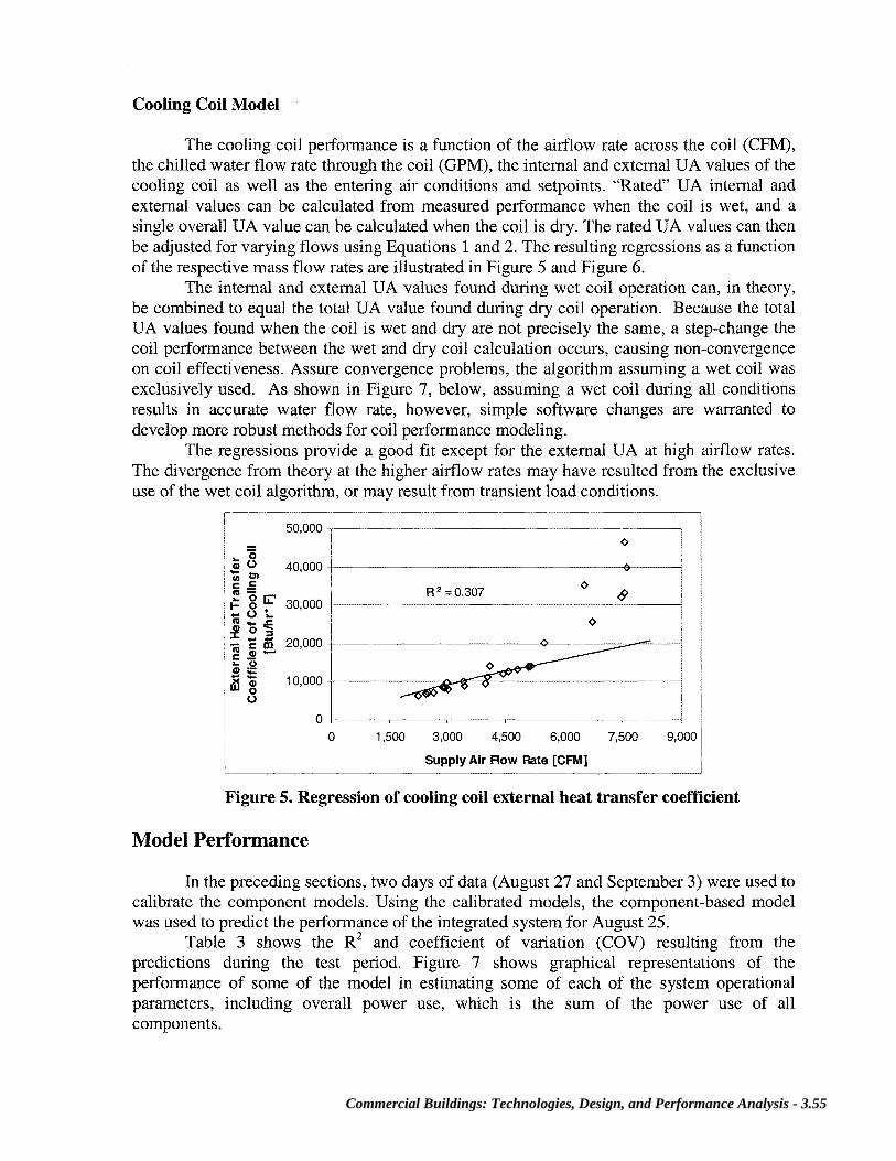
The cooling coil performance is a function of the airflow rate across the coil (CFM),the chilled water flow rate through the coil (GPM), the internal and external UA values of thecooling coil as well as the entering air conditions and setpoints. “Rated” UA internal andexternal values can be calculated from measured performance when the coil is wet, and asingle overall UA value can be calculated when the coil is dry. The rated UA values can thenbe adjusted for varying flows using Equations 1 and 2. The resulting regressions as a functionof the respective mass flow rates are illustrated in Figure 5 and Figure 6.

The internal and external UA values found during wet coil operation can, in theory,be combined to equal the total UA value found during dry coil operation. Because the totalUA values found when the coil is wet and dry are not precisely the same, a step-change thecoil performance between the wet and dry coil calculation occurs, causing non-convergenceon coil effectiveness. Assure convergence problems, the algorithm assuming a wet coil wasexclusively used. As shown in Figure 7, below, assuming a wet coil during all conditionsresults in accurate water flow rate, however, simple software changes are warranted todevelop more robust methods for coil performance modeling.

The regressions provide a good fit except for the external UA at high airflow rates.The divergence from theory at the higher airflow rates may have resulted from the exclusiveuse ofthe wet coil algorithm, or may result from transient load conditions.

50,0000

a-°~ ~ 40,000

R2=0.307~‘ 30,000

0

0 1,500 3,000 4,500 6,000 7,500 9,000

Supply Air Flow Rate (CFMI

Figure 5. Regression of cooling coil external heat transfer coefficient

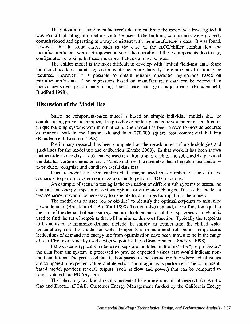
Model Performance

In the preceding sections, two days of data (August 27 and September 3) were used tocalibrate the component models. Using the calibrated models, the component-based modelwas used to predict the performance ofthe integrated system for August 25.

Table 3 shows the R2 and coefficient of variation (COV) resulting from thepredictions during the test period. Figure 7 shows graphical representations of theperformance of some of the model in estimating some of each of the system operationalparameters, including overall power use, which is the sum of the power use of allcomponents.

Commercial Buildings: Technologies, Design, and Performance Analysis - 3.55

40,000

L~’ 35,000 0.~

° 30,000R2=0.786

~ 25,000.-0 =~ 0 20,000

~ 15,000=

10,000

5000 0

00 20 40 60 80 100

Chilled Water Flow Rate [GPM]

Figure 6. Regression of cooling coil internal heat transfer coefficient.

Table 3. Test data prediction results by building system componentComponent R2 COY (%)Supply Air Fan Power Consumption 0.992 4.02Secondary Chilled Water Pump Power Consumption 0.979 1.16Chiller Power Consumption 0.894 16.30Air-Cooled Condenser Power Consumption 0.0835 18.32Chilled Water Flow Rates 0.978 4.52Overall System Power Consumption 0.889 12.13

Considering the restricted amount of data used for calibration, the results are good inthe well-controlled conditions of the laboratory. The components that had rather high COVwere the chiller and the ACC. The chiller COV was high because the two days of power dataof the chiller were not representative of the higher operating range, which was obtained onthe third day. The ACC was high because the power consumption was being predicted on acomponent that is a constant power device. Therefore, the graphical plot of predicted versusactual performance should be a tight cluster of points, which is observable with the majorityof the data in Figure 7.

Training data

When calculating the coefficients, it was found that the quality of data was moreimportant then the quantity of data. The data used to calculate the various coefficients needsto cover a representative subset of the expected operational range. Large data sets can beavoided, and gaps in the training set can be tolerated, however, since the shape of the variouscurves is generally known a priori and manufacturer’s data can be used in many cases forcoils, ACCs, and chillers.

Generally, the best time to collect the data would be when the cooling system’scomponents are operating at a variety ofranges (i.e., during the summer or swing months). Itis possible to calibrate the model successfully using as little as one day’s worth of data if theycover a reasonably broad range of operation.

3.56

The potential of using manufacturer’s data to calibrate the model was investigated. Itwas found that rating information could be used if the building components were properlycommissioned and operating in a way consistent with the manufacturer’s data. It was found,however, that in some cases, such as the case of the ACC/chiller combination, themanufacturer’s data were not representative of the operation if these components due to age,configuration or sizing. In these situations, field data must be used.

The chiller model is the most difficult to develop with limited field-test data. Sincethe model has ten separate regression coefficients, a relatively large amount of data may berequired. However, it is possible to obtain reliable quadratic regressions based onmanufacturer’s data. The regressions based on manufacturer’s data can be corrected tomatch measured performance using linear base and gain adjustments (Brandemuehl,Bradford 1998).

Discussion of the Model Use

Since the component-based model is based on simple individual models that arecoupled using proven techniques, it is possible to build-up and calibrate the representation forunique building systems with minimal data. The model has been shown to provide accurateestimations both in the Larson lab and in a 270,000 square foot commercial building(Brandemuehl, Bradford 1998).

Preliminary research has been completed on the development of methodologies andguidelines for the model use and calibration (Zarske 2000). In that work, it has been shownthat as little as one day of data can be used in calibration of each of the sub-models, providedthe data has certain characteristics. Zarske outlines the desirable data characteristics and howto produce, recognize and condition useful data sets.

Once a model has been calibrated, it maybe used in a number of ways: to testscenarios, to perform system optimization, and to perform FDD functions.

An example of scenario testing is the evaluation of different sub systems to assess thedemand and energy impacts of various options or efficiency changes. To use the model totest scenarios, it would be necessary to generate load profiles for input into the model.

The model can be used (on or off-line) to identify the optimal setpoints to minimizepower demand (Brandemuehi, Bradford 1998). To minimize demand, a cost function equal tothe sum of the demand of each sub system is calculated and a solution space search method isused to find the set of setpoints that will minimize this cost function. Typically the setpointsto be adjusted to minimize demand include the supply air temperature, the chilled watertemperature, and the condenser water temperature or saturated refrigerant temperature.Reductions of demand and energy use from optimization have been shown to be in the rangeof 5 to 10% over typically used design setpoint values (Brandemuehl, Bradford 1998).

FDD systems typically include two separate modules, in the first, the “pre-processor,”the data from the system is processed to provide expected values that would indicate non-fault conditions. The processed data is then passed to the second module where actual valuesare compared to expected values and detection and diagnosis is performed. The component-based model provides several outputs (such as flow and power) that can be compared toactual values in an FDD system.

The laboratory work and results presented herein are a result of research for PacificGas and Electric (PG&E) Customer Energy Management funded by the California Energy

Commercial Buildings: Technologies, Design, and Performance Analysis - 3.57

Commission (CEC) (PG&E et al., 1999). The support of PG&E and the CEC are gratefullyacknowledged.

2nd Chilled Water Flow Rate

R2=O,978~40

20

(~00 20 40 60 80

GPM Actual

2.5t 2.0-a0I-

°- 1.00,50.0

Chiller

25R~-08

o 201510

~—

I00 5 10 15 20 25

kWActual

Supply Air Fans

2.5-ao‘t; 2.0

~0C,~ 1.0

.~0.5

0.0

R2= 0.992

~v— -

~—

—----~

0.0 0.5 1.0 1.5 2.0 2.IkW Actual

Total Power

30~25 R2=0.889~ 20~15& 10

—

.~

0~T0 5 10 15 20 25 30

kW Actual

Figure 7. Predicted versus actual model performance

Air-Cooled Condenser

3.0

0.0 0.5 1.0 1.5 2.0 2.5 3.~kW Actual

v

~-

~~-~

2nd Chilled Water Pump

1.5R2=0.979

~

0.60.3

—

0.0 ~

0.0 0.3 0.6 0.9 1.2 1kWActual

References

Brandemuehl, Bradford, J.D. 1998. Implementation of On-line Optimal Supervisory Controlof Cooling Plants Without Storage, Draft final report for ASHRAE Research Project823-RP. JCEM TR/98/3, Department of Civil, Environmental, and ArchitecturalEngineering, University of Colorado, Boulder.

Brandemuehi, M. J.,1992, HVAC 2 Toolkit, The American Society of Heating, Refrigeratingand Air Conditioning Engineers (ASHRAE), Atlanta, GA

3.58

Braun, J.E., 1988, Methodologies for the Design and Control of Central Cooling Plants,Ph.D. Dissertation, Department of Mechanical Engineering, University of Wisconsin-Madison

Braun, J.E., and Diderrich, G.T., 1990, “Near Optimal control of Cooling Towers for ChilledWater Systems.” ASHRAE Transactions, Volume 96, Part 2

Braun, Klein, Beckman, Mitchell, 1989, “Methodologies for Optimal Control of ChilledWater System Without Storage”, ASHRAE Transactions, Volume 95, Part 1 (RP-539)

Braun, Mitchell, Klein, Beckman, 1987, “Performance and Control Characteristics of a LargeCooling System”, ASHRAE Transactions, NY 87-22-4 (RP-409)

Culmi, 1988, “Global Optimization of HVAC System Operations in Real Time,” ASHRAETransactions, Volume 94, Part 1

LBL, 1980, “DOE2 User Guide, Version 2.1”, Lawrence Berkeley Laboratory and LosAlamos National Laboratory, LBL Report No. LBL-8689 Revision 2, DOE2 UserCoordination Office, LBL, Berkeley, California

Kreider, Jan F., Peter S. Curtiss, Darrell Massie, and Erik Jeannette. 1999. “A Commercial-Scale University HVAC Laboratory.” ASHRAE Transactions, Volume 105, Part 1.

Liu, M. and Claridge, D.E., “Use of Calibrated HVAC System Models to Optimize SystemOperation,” ASME Journal ofSolar Energy Engineering, Vol 120, pp. 131-138, 1998

Pacific Gas and Electric Company, Schiller Associates, Energy Simulation Specialists, JointCenter for Energy Management, 1999, Improving The Cost Effectiveness OfBuildingDiagnostics, Measurement And Commissioning Using New Techniques ForMeasurement, Verification And Analysis, California Energy Commission, CaliforniaEnergy Commission, Public Energy Interest Research Program, Sacramento, CA95814

Phelan, J, Brandemuehl, M.J., and Krarti, M. 1997. “In-Situ Performance Testing of ChillersforEnergy Analysis.” ASHRAE Transactions, Volume 103, Part 1.

Threlkeld, J.L. 1970. Thermal Environmental Engineering.2

nd Edition, Prentice-Hall, Inc.,Englewood Cliffs, New Jersey.

Phelan, J, Brandemuehl, M. J., and Krarti, M. 1996, Draft Guidelines for In-SituPerformance Testing of Centrifugal Chillers, for ASHRAE Research Project 827-RP,Joint Center for Energy Management, Department of Civil, Architectural andEnvironmental Engineering, University of Colorado, Boulder

Zarske, J.N. 2000 Component-based Modeling of Cooling Systems Using Short-term DataMS Thesis, Department of Civil Engineering, University of Colorado, Boulder

Commercial Buildings: Technologies, Design, and Performance Analysis - 3.59

3.60