First Baby Steps in AnalyzingSTEREO/EUVI Images

Markus J. AschwandenJim Lemen, Jean-Pierre Wuelser, & Nariaki Nitta

(LMSAL)

5th SECCHI Consortium Meeting University Paris-Sud, Orsay

March 5-8, 2007

Content:

1) EUVI Observing Sequence2) EUVI Cadence vs. GOES light curve3) EUVI full resolution images4) EUVI image compression5) GOES flare events: 2006/Dec-2007/Feb6) CME/occulted flare event 2007-Jan-24 14 UT7) Future EUVI data analysis goals8) Strategies for EUVI observations

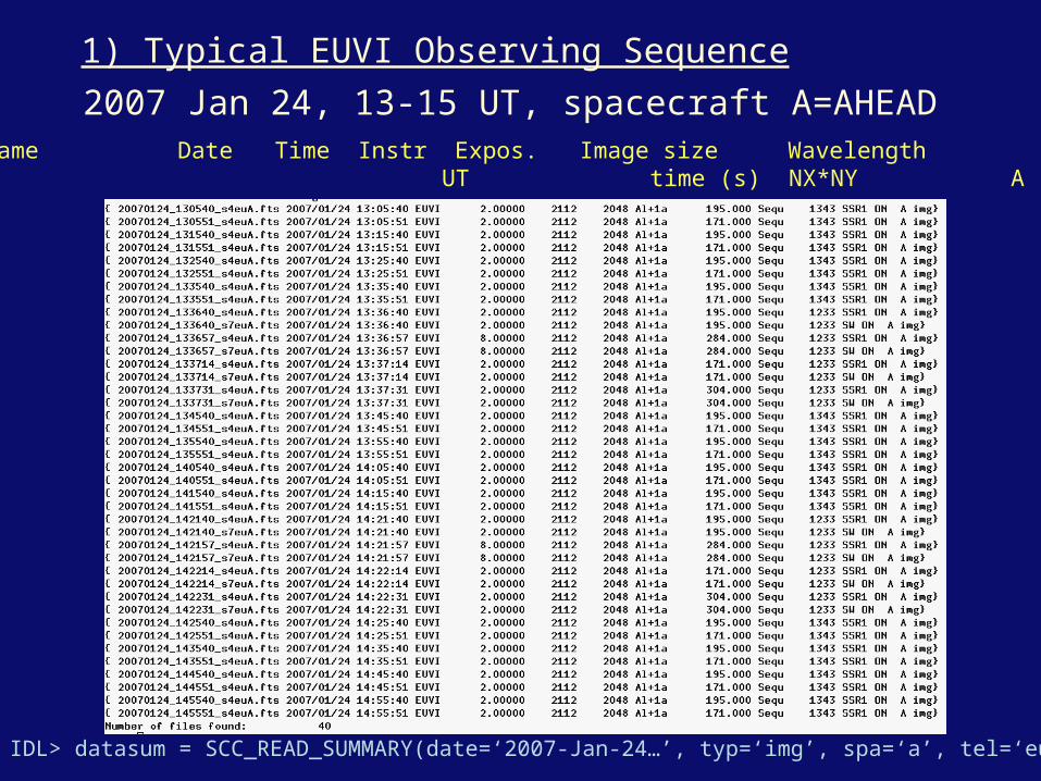
1) Typical EUVI Observing Sequence

2007 Jan 24, 13-15 UT, spacecraft A=AHEADFilename Date Time Instr Expos. Image size Wavelength UT time (s) NX*NY A

IDL> datasum = SCC_READ_SUMMARY(date=‘2007-Jan-24…’, typ=‘img’, spa=‘a’, tel=‘euvi’)

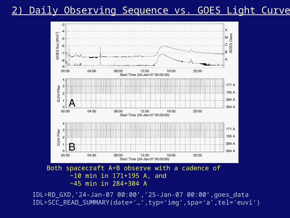
2) Daily Observing Sequence vs. GOES Light Curve

Both spacecraft A+B observe with a cadence of ~10 min in 171+195 A, and ~45 min in 284+304 A

IDL>RD_GXD,’24-Jan-07 00:00’,’25-Jan-07 00:00’,goes_dataIDL>SCC_READ_SUMMARY(date=‘…’,typ=‘img’,spa=‘a’,tel=‘euvi’)

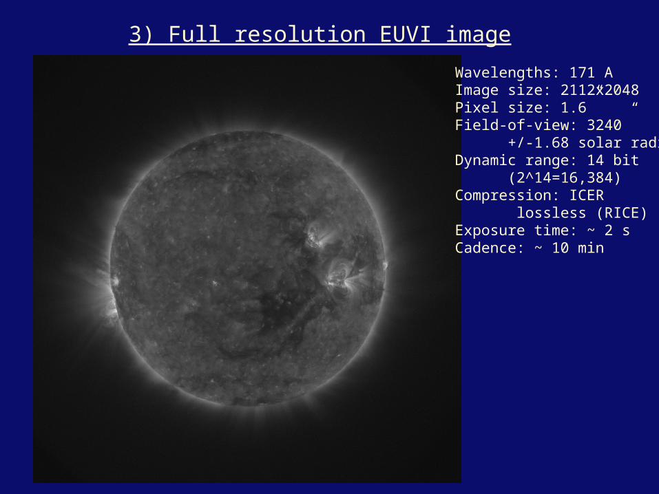
3) Full resolution EUVI image

Wavelengths: 171 AImage size: 2112x2048Pixel size: 1.6”Field-of-view: 3240” +/-1.68 solar radiiDynamic range: 14 bit (2^14=16,384)Compression: ICER lossless (RICE)Exposure time: ~ 2 sCadence: ~ 10 min

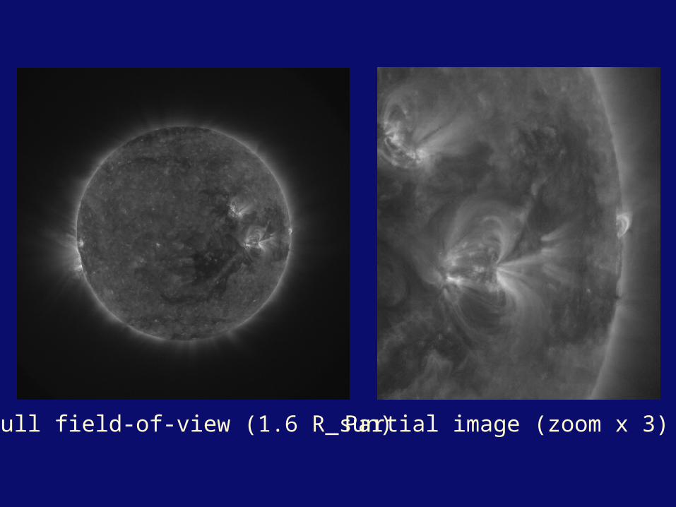
Full field-of-view (1.6 R_sun) Partial image (zoom x 3)

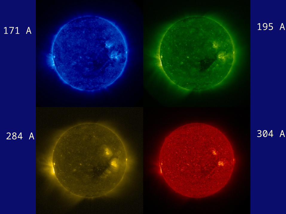
171 A

284 A

195 A

304 A

4) Image Compression

EUVI 171 A imageSegment (East sector)i=0:512, j=831:1031

Flux profileF(i=0:512, j=931) DN

Difference of flux profilebetween compressedICER4 and lossless RICEdF=+/-2.7 … +/-4.7 DN

Difference normalizedby Poisson noise:dF/s=+/-0.8 … 0.6(not significant !)

EUVI 171 A imageSegment (East sector)i=0:512, j=831:1031

Flux profileF(i=0:512, j=931) DN

Difference of flux profilebetween compressedICER6 and lossless RICEdF=+/-2.8 … +/-5.8 DN

Difference normalizedby Poisson noise:dF/s=+/-0.9 … 0.7(not significant !)

ICER 4:Difference dF/s=0.8…0.6

ICER 6:Difference dF/s=0.9…0.7

No significant difference in compression quality

EUVI 171 A image

Difference normalizedby Poisson noise:dF/s=-1 … +1 (black … white)

ICER 4

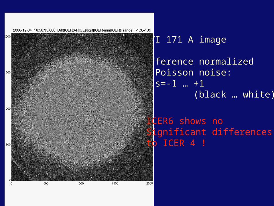
EUVI 171 A image

Difference normalizedby Poisson noise:dF/s=-1 … +1 (black … white)

ICER6 shows noSignificant differencesto ICER 4 !

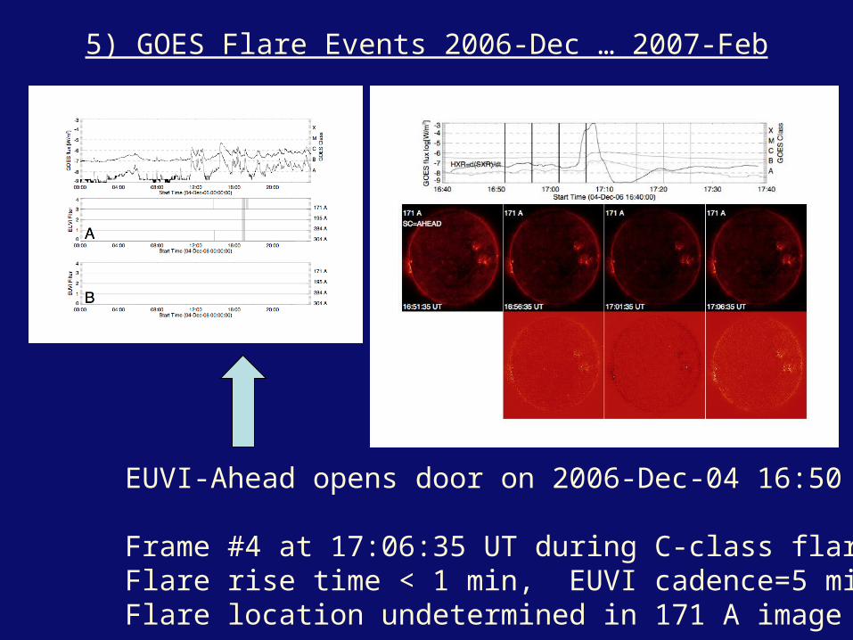
5) GOES Flare Events 2006-Dec … 2007-Feb

EUVI-Ahead opens door on 2006-Dec-04 16:50 UT

Frame #4 at 17:06:35 UT during C-class flareFlare rise time < 1 min, EUVI cadence=5 minFlare location undetermined in 171 A image

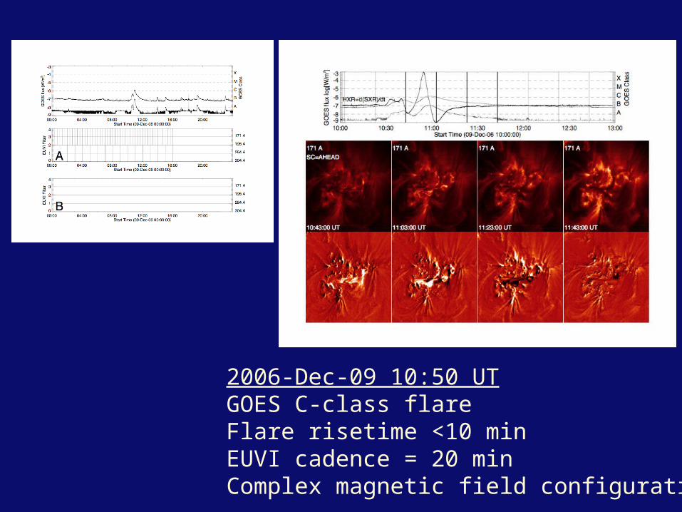
2006-Dec-09 10:50 UTGOES C-class flareFlare risetime <10 minEUVI cadence = 20 minComplex magnetic field configuration

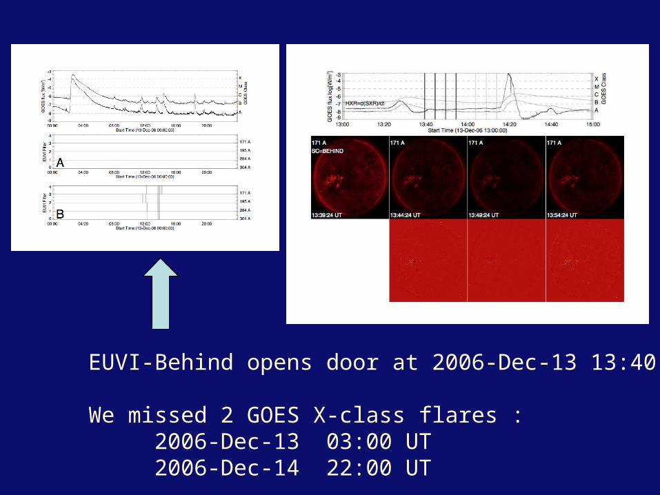
EUVI-Behind opens door at 2006-Dec-13 13:40 UT

We missed 2 GOES X-class flares : 2006-Dec-13 03:00 UT2006-Dec-14 22:00 UT

GOES C-class flare 2006-Dec-31 07:00 UTFlare rise time < 10 minEUVI cadence A: 171,195=20 min, B: 195,304=5 minQuadrupolar double-arcade flare system

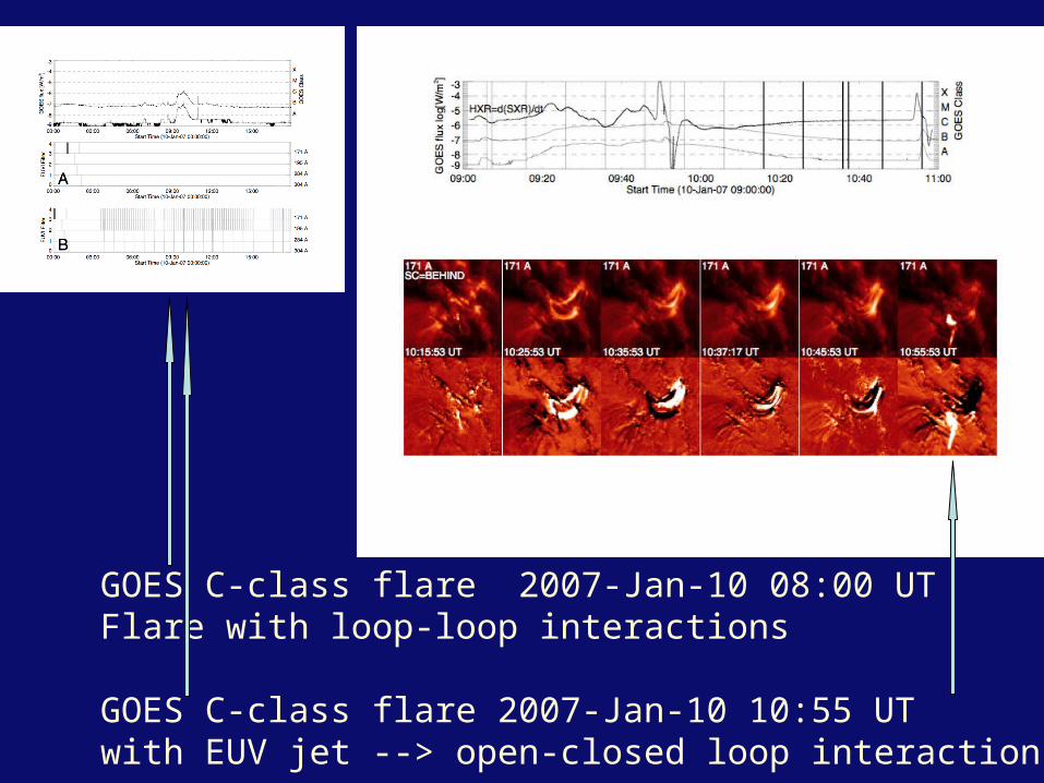
GOES C-class flare 2007-Jan-10 08:00 UT Flare with loop-loop interactions

GOES C-class flare 2007-Jan-10 10:55 UT with EUV jet --> open-closed loop interaction

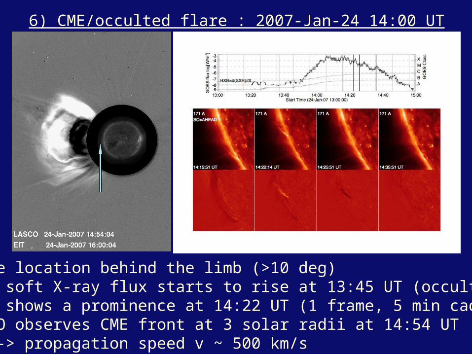
6) CME/occulted flare : 2007-Jan-24 14:00 UT

Flare location behind the limb (>10 deg)GOES soft X-ray flux starts to rise at 13:45 UT (occulted)EUVI shows a prominence at 14:22 UT (1 frame, 5 min cadence)LASCO observes CME front at 3 solar radii at 14:54 UT --> propagation speed v ~ 500 km/s

Flare start ~ 13:35 UTAR loops are shakenby filament eruptionand first brighteningabove limb, while flarelocation is occulted,GOES light curve startsto increase at 13:50 UT

Flare peak ~ 14:05 UTAR loops are shakenstrongest (dampedoscillations ?), but all postflare loops are still occulted,GOES light curveshows steepestincrease (HXR max)at 14:10 UT

+2 hrs later: Postflare loop expands behind limb and the top of the arcade becomes visible

+4 hrs later: Postflare loop system expands higher and EM of postflare loops still increases

+ 6 hrs: Post flare loops expand higher

+ 9 hrs:

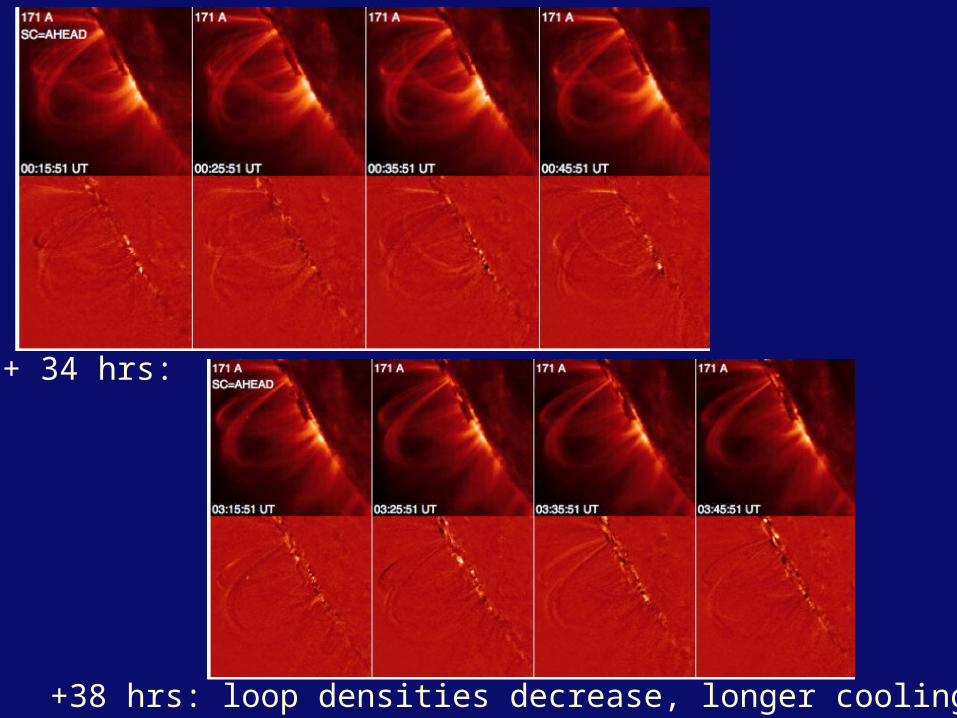
+ 34 hrs:

+38 hrs: loop densities decrease, longer cooling times

13:35 UT flare start (GOES increase, EUVI loop shaking)

14:05 UT flare peak (GOES steepest increase, EUVI loop oscillations)14:22 UT: EUVI prominence/eruptive filament appears LASCO: CME front appears at >1 solar radii

15:00 UT: LASCO: CME front propagates > 3 solar radii with a speed of v~500 km/s

16:05 UT: EUVI: Postflare loop system appears above limb

18:15 UT: EUVI: Postflare loops h=19 Mm, v=2.4 km/s20:15 UT: EUVI: Postflare loops h=40 Mm, v=2.6 km/s

23:15 UT: EUVI: Postflare loops h=70 Mm, v=2.7 km/s

+34,38 hrs: EUVI postflare loop still visible h>100 Mm

7) Future EUVI Data Analysis Goals

SoHO/LASCO Team

a) Determine 3D Magnetic field geometry at CME initiation site

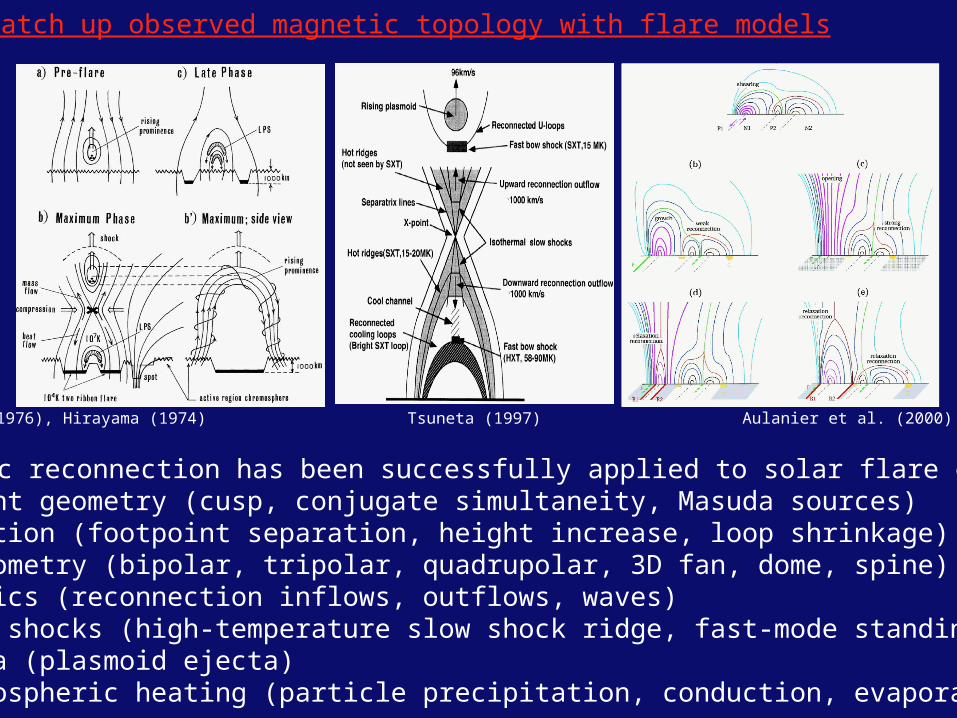
Magnetic reconnection has been successfully applied to solar flare events:X-point geometry (cusp, conjugate simultaneity, Masuda sources)Evolution (footpoint separation, height increase, loop shrinkage)3D geometry (bipolar, tripolar, quadrupolar, 3D fan, dome, spine)Dynamics (reconnection inflows, outflows, waves)Flare shocks (high-temperature slow shock ridge, fast-mode standing shock)Ejecta (plasmoid ejecta)Chromospheric heating (particle precipitation, conduction, evaporation)

Kopp & Pneumann (1976), Hirayama (1974) Tsuneta (1997) Aulanier et al. (2000)

b) Match up observed magnetic topology with flare models

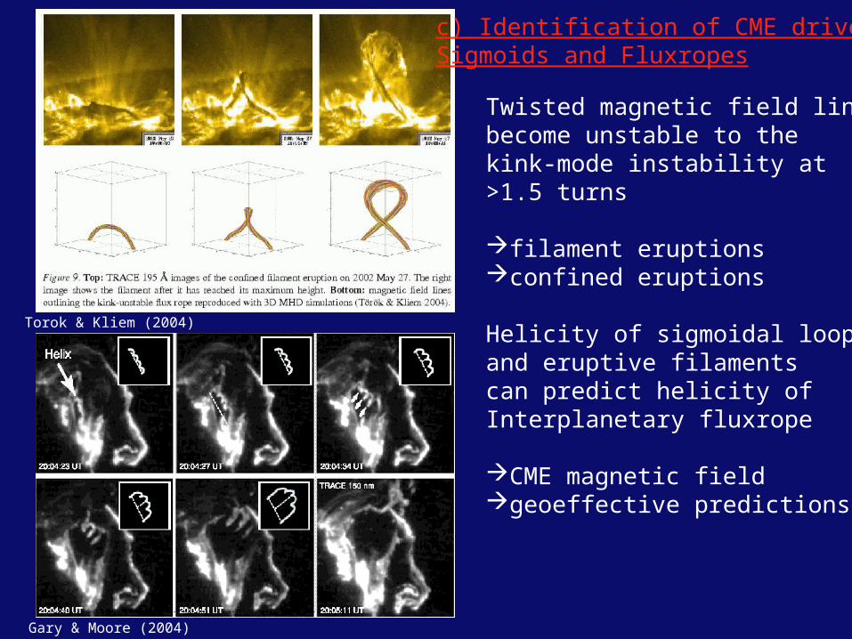
Twisted magnetic field linesbecome unstable to thekink-mode instability at>1.5 turns

filament eruptionsconfined eruptions

Helicity of sigmoidal loopsand eruptive filamentscan predict helicity ofInterplanetary fluxrope

CME magnetic fieldgeoeffective predictions

Torok & Kliem (2004)

Gary & Moore (2004)

c) Identification of CME drivers:Sigmoids and Fluxropes

Amary et al. (2003)

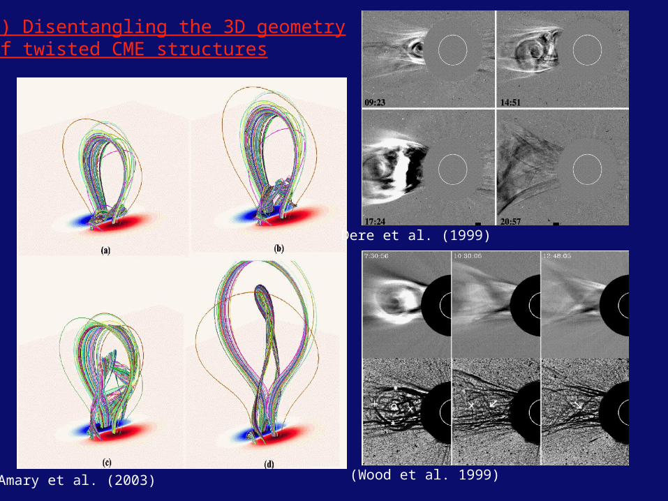
d) Disentangling the 3D geometryof twisted CME structures

Dere et al. (1999)

(Wood et al. 1999)

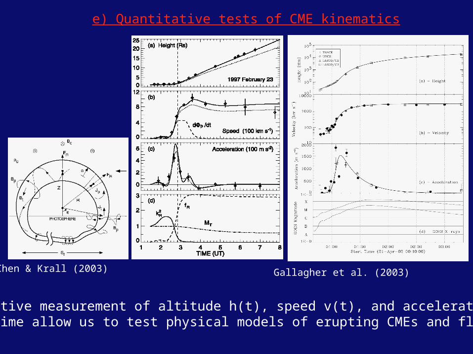
Gallagher et al. (2003)Chen & Krall (2003)

Quantitative measurement of altitude h(t), speed v(t), and acceleration a(t)Versus time allow us to test physical models of erupting CMEs and fluxropes.

e) Quantitative tests of CME kinematics

Aschwanden et al. (2001)

McLean & Sheridan (1973)

Wang et al. (2003)

Verwichte et al. (2004)

f) Study oscillatory dynamics after filament eruption or CME launch

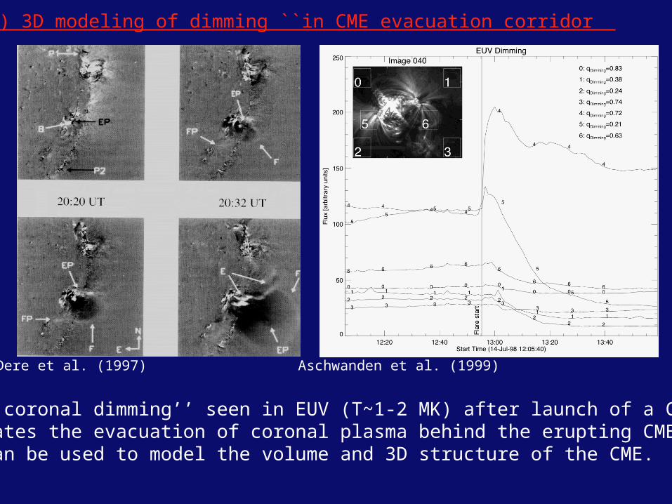
Dere et al. (1997) Aschwanden et al. (1999)

The ``coronal dimming’’ seen in EUV (T~1-2 MK) after launch of a CMEIndicates the evacuation of coronal plasma behind the erupting CMEand can be used to model the volume and 3D structure of the CME.

g) 3D modeling of dimming ``in CME evacuation corridor”

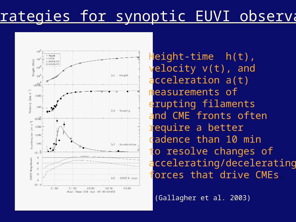
7) Strategies for synoptic EUVI observations

Height-time h(t),velocity v(t), andacceleration a(t)measurements oferupting filaments and CME fronts oftenrequire a better cadence than 10 minto resolve changes ofaccelerating/deceleratingforces that drive CMEs.

(Gallagher et al. 2003)

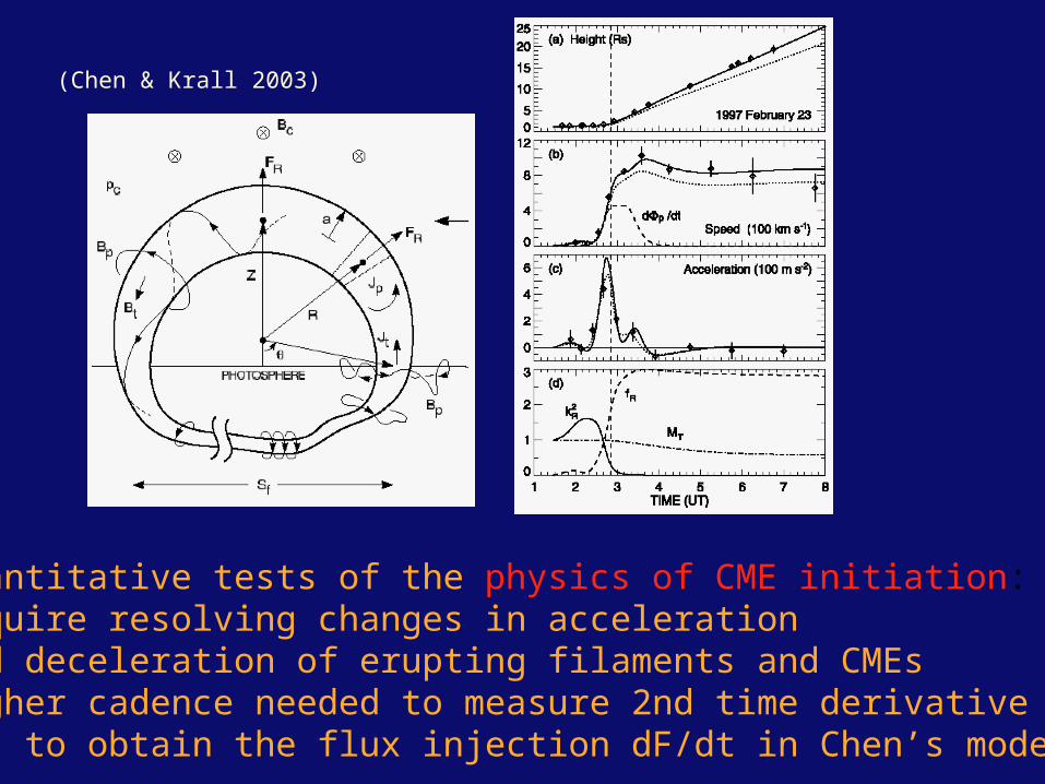
Quantitative tests of the physics of CME initiation:require resolving changes in accelerationand deceleration of erupting filaments and CMEshigher cadence needed to measure 2nd time derivative to obtain the flux injection dF/dt in Chen’s model

(Chen & Krall 2003)

(Dere et al. 1997)

An erupting filamentor CME front clearsthe EUVI FOV within

t=h/v~8-30 min

(h=500,000 km v=300…1000 km/s)

With a typical EITcadence of 10 minwe miss all fasterCMEs and obtainonly ~2 imagesfor slow CMEsinsufficient contextfor modeling dimming

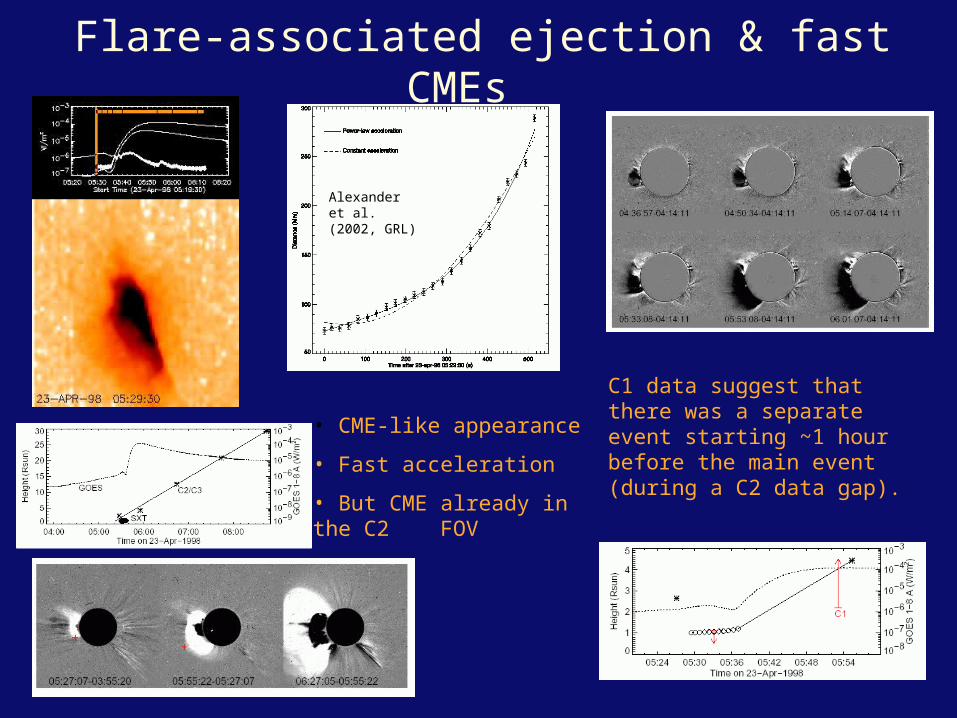
Flare-associated ejection & fast CMEs

• CME-like appearance

• Fast acceleration

• But CME already in the C2 FOV

C1 data suggest that there was a separate event starting ~1 hour before the main event (during a C2 data gap).

Alexander et al. (2002, GRL)

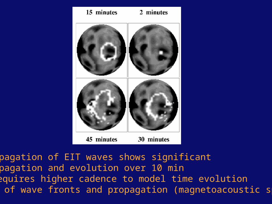
Propagation of EIT waves shows significantpropagation and evolution over 10 minrequires higher cadence to model time evolution of wave fronts and propagation (magnetoacoustic speed)

Strategy 1) Fast-cadence 171 images:

-Fast cadence of 2.5 min benefits science ofdynamic “CME initiation” phenomena(filament eruption, dimming, EIT waves, etc. velocity & acceleration measurements)

-Low 10-min cadence is insufficient to resolve dynamicchanges in EUVI FOV

(EIT missed most eruptive filaments or got only 1 frame)

-Fast cadence can be afforded with higher compression(ICER6 uses a factor of 2 less telemetry than ICER4)

Difference in photon statistics of ICER6 vs. ICER4is not significant !

Strategy 2: High cadence in 171 A rather than 195 A:

171 TRACE movies show filament eruption (in absorption) very well at <1.1…1.2 solar radii during initiation of CME

AR (loop) structures are crispier in 171 than in 195 A, during pre-CME conditioning.

EIT has tracked EIT waves dominantly in 195 A, but there is no statistical evidence that EIT waves are better detected in 195 A than in 171 A

Conclusions:

1) Current focus in developing EUVI data analysis software :- Image quality (compression, exposure time, cadence)- Image calibration (flatfielding, flux-EM conversion, intercalibration)

- Image coalignment (spacecraft pointing, roll angle correction)- Visualization (browser, movies, overlays; FESTIVAL, PANORAMA)- 3D Geometric reconstruction from 2 stereoscopic views

2) Data analysis during first 3 months (Dec 2006-Feb 2007): - Stereoscopic separation angle <1.2 deg at March 1, 2007

- EUVI observed 1 CME (2007-02-14) and about a dozen C-flares - shaking and damped oscillations of coronal loops at CME launch

- quiescent and erupting filaments/prominences - bipolar, tripolar (jets), and quadrupolar flare configurations - evolution of postflare loop systems

3) Strategy of future EUVI synoptic observations: - increase cadence of 171 A from 10 min to 2.5 min - choose 171 for fast cadence rather than 195

New EUVI website:

http://secchi.lmsal.com/EUVI/