Firms, Production Possibility Sets, and ProfitMaximization

Econ 2100, Fall 2019

Lecture 1, 21 October

Outline

1 Logistics2 Production Sets and Production Functions3 Profits Maximization, Supply Correspondence, and Profit Function

Logistics

Instructor: Luca RigottiOffi ce: WWPH 4115, email: luca at pitt.eduOffi ce Hours: Friday 2:30pm-4pm, or by appointment (send me an email)

Teaching Assistant: Yunyun LvOffi ce: WWPH 4518, email: yul197@pitt.eduOffi ce Hours: TBA, Monday 2-4pm.

Class Time and LocationMonday & Wednesday, 10:30am to 11:45am in WWPH 4940Recitation TimesFriday, 2pm to 3:15am, in WWPH 4940.

Class Webpage http://www.pitt.edu/~luca/ECON2100/

AnnouncementsNone Today

LogisticsHandouts: For each class, I will post an handout that you can use to take notes(either print and bring to class, or use computer).

Textbooks: Kreps, Microeconomic Foundations I: Choice and CompetitiveMarkets, Princeton University PressMas-Collel, Whinston and Green: Microeconomic Theory.Other useful textbooks by Varian, Jehle and Reny, older Kreps.My favorite: Gerard Debreu: Theory of Value.

Grading

Luca’s Half: Problem set 10%, Exam 90%Final Exam, 2 hours long, date TBA

Problem SetsWeekly, some questions appear during class.DO NOT look for answers... These are for you to learn what you can andcannot do; we can help you get better only if we know your limits.Working in teams strongly encouraged, but turn in problem sets individually.Start working on exercises on your own, and then get together to discuss.Typically, a Problem Set will be due at the beginning of each Monday class.

Luca’s Goals for Micro Theory Sequence

Learn and understand the microeconomic theory every academic economistneeds to know.

Stimulate interest in micro theory as a field (some of you may want to becometheorists).

Enable you to read papers that use theory, and go to research seminars.

We will cover the following standard topics:

firms: production, profit maximization, aggregation;general equilibrium theory: consumers and firms in competitive markets,Walrasian equilibrium, First and Second Welfare Theorems, existence ofequilibrium, uniqueness of equilibrium, markets with uncertainty and time,Arrow-Debreu economies.

In the Spring, Professor Richard van Weelden will cover game theory andinformation economics.

Questions? This will be fun: let’s go!

Producers and Production SetsProducers are profit maximizing firms that buy inputs and use them to produce andthen sell outputs.

The plural is important because most firms produce more than one good.

The standard undergraduate textbook description focuses on one ouput and afew inputs (two in most cases).

In that framework, production is described by a function that takes inputs asthe domain and output(s) as the range.

Here we focus on a more general and abstract version of production.

DefinitionA production set is a subset Y ⊆ Rn .

y = (y1, ..., yN ) denotes production (input-output) vectors.

A production vector has outputs as non-negative numbers and inputs asnon-positive numbers: yi ≤ 0 when i is an input, and yi ≥ 0 if i is an output.What is p · y in this notation?

Production Set Properties

DefinitionY ⊆ Rn satisfies:

no free lunch if Y ∩ Rn+ ⊆ {0n};possibility of inaction if 0n ∈ Y ;free disposal if y ∈ Y implies y ′ ∈ Y for all y ′ ≤ y ;irreversibility if y ∈ Y and y 6= 0n imply −y /∈ Y ;nonincreasing returns to scale if y ∈ Y implies αy ∈ Y for all α ∈ [0, 1];

nondecreasing returns to scale if y ∈ Y implies αy ∈ Y for all α ≥ 1;constant returns to scale if y ∈ Y implies αy ∈ Y for all α ≥ 0;additivity if y , y ′ ∈ Y imply y + y ′ ∈ Y ;convexity if Y is convex;

Y is a convex cone if for any y , y ′ ∈ Y and α, β ≥ 0, αy + βy ′ ∈ Y .

Draw Pictures.

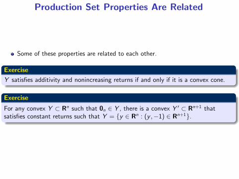
Production Set Properties Are Related

Some of these properties are related to each other.

ExerciseY satisfies additivity and nonincreasing returns if and only if it is a convex cone.

Exercise

For any convex Y ⊂ Rn such that 0n ∈ Y , there is a convex Y ′ ⊂ Rn+1 thatsatisfies constant returns such that Y = {y ∈ Rn : (y ,−1) ∈ Rn+1}.

Production FunctionsLet y ∈ Rm+ denote outputs while x ∈ Rn+ represent inputs; if the two are related bya function f : Rn+ → Rm+, we write y = f (x) to say that y units of outputs areproduced using x amount of the inputs.

When m = 1, this is the familiar one output many inputs production function.

Production sets and the familiar production function are related.

ExerciseSuppose the firm’s production set is generated by a production functionf : Rn+ → Rm+, where Rn+ represents its n inputs and R+ represents its m outputs.Let

Y = {(−x , y) ∈ Rn− × Rm+ : y ≤ f (x)}.Prove the following:

1 Y satisfies no free lunch, possibility of inaction, free disposal, and irreversibility.2 Suppose m = 1. Y satisfies constant returns to scale if and only if f ishomogeneous of degree one, i.e. f (αx) = αf (x) for all α ≥ 0.

3 Suppose m = 1. Y satisfies convexity if and only if f is concave.

Transformation FunctionWe can describe production sets using a function.

DefinitionGiven a production set Y ⊆ Rn , the transformation function F : Y → R is definedby

Y = {y ∈ Y : F (y) ≤ 0 and F (y) = 0 if and only if y is on the boundary of Y } ;

the transformation frontier is{y ∈ Rn : F (y) = 0}

DefinitionGiven a differentiable transformation function F and a point on its transformationfrontier y , the marginal rate of transformation for goods i and j is given by

MRTi ,j =

∂F (y )∂yi∂F (y )∂yj

Since F (y) = 0 we have∂F (y)

∂yidyi +

∂F (y)

∂yjdyj = 0

MRT is the slope of the transformation frontier at y .

Profit Maximization

Profit Maximizing AssumptionThe firm’s objective is to choose a production vector on the trasformation frontieras to maximize profits given prices p ∈ Rn++:

maxy∈Y

p · y

or equivalentlymax p · y subject to F (y) ≤ 0

Does this distinguish between revenues and costs? How?

Using the single output production function:maxx≥0

pf (x)− w · x

here p ∈ R++ is the price of output and w ∈ Rl++ is the price of inputs.

First Order Conditions For Profit Maximization

max p · y subject to F (y) = 0

Profit MaximizingThe FOC are

pi = λ∂F (y)

∂yifor each i or p︸︷︷︸

1×n

= λ∇F (y)︸ ︷︷ ︸1×n

in matrix form

Therefore1λ

=

∂F (y )∂yi

pifor each i

the marginal product per dollar spent or received is equal across all goods.

Using this formula for i and j :∂F (y )∂yi∂F (y )∂yj

= MRTi ,j =pipjfor each i , j

the Marginal Rate of Transformation equals the price ratio.

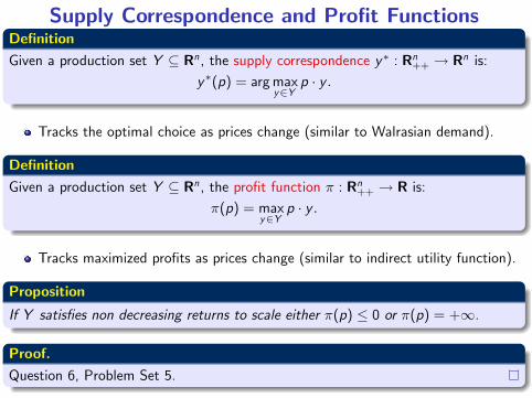
Supply Correspondence and Profit FunctionsDefinitionGiven a production set Y ⊆ Rn , the supply correspondence y∗ : Rn++ → Rn is:

y∗(p) = argmaxy∈Y

p · y .

Tracks the optimal choice as prices change (similar to Walrasian demand).

DefinitionGiven a production set Y ⊆ Rn , the profit function π : Rn++ → R is:

π(p) = maxy∈Y

p · y .

Tracks maximized profits as prices change (similar to indirect utility function).

Proposition

If Y satisfies non decreasing returns to scale either π(p) ≤ 0 or π(p) = +∞.

Proof.Question 6, Problem Set 5.

Properties of Supply and Profit Functions

PropositionSuppose Y is closed and satisfies free disposal. Then:

π(αp) = απ(p) for all α > 0;

π is convex in p;

y∗(αp) = y∗(p) for all α > 0;

if Y is convex, then y∗(p) is convex;

if |y∗(p)| = 1, then π is differentiable at p and ∇π(p) = y∗(p) (Hotelling’sLemma).

if y∗(p) is differentiable at p, then Dy∗(p) = D2π(p) is symmetric andpositive semidefinite with Dy∗(p)p = 0.

The Profit Function Is Convex

Proof.

Let p,p′ ∈ Rn++ and let the corresponding profit maximizing solutions be y and y′.

For any λ ∈ (0, 1) let p = λp + (1− λ) p′ and let y be the profit maximizingoutput vector when prices are p.

By “revealed preferences”

p · y ≥ p · y and p′ · y ′ ≥ p′ · ywhy?

multiply these inequalities by λ and 1− λλp · y ≥ λp · y and (1− λ) p′ · y ′ ≥ (1− λ) p′ · y

summing up

λp · y + (1− λ) p′ · y ′ ≥ [λp + (1− λ) p′] · yusing the definition of profit function:

λπ (p) + (1− λ)π (p′) ≥ π (λp + (1− λ) p′)proving convexity of π (p).

The Supply Correspondence Is Convex

Proof.

Let p ∈ Rn++ and let y , y′ ∈ y∗(p).

We need to show that if Y is convex then

λy + (1− λ) y ′ ∈ y∗(p) for any λ ∈ (0, 1)

By definition:p · y ≥ p · y for any y ∈ Y and p · y ′ ≥ p · y for any y ∈ Y

multiplying by λ and 1− λ we getλp · y ≥ λp · y and (1− λ) p · y ′ ≥ (1− λ) p · y

Therefore, summing up, we have

λp · y + (1− λ) p · y ′ ≥ [λ+ (1− λ)] p · yRearranging:

p · [λy + (1− λ) y ′] ≥ p · yproving convexity of y∗(p).

Hotelling’s Lemmaif |y∗(p)| = 1, then π is differentiable at p and ∇π(p) = y∗(p)

Proof.

Suppose y∗(p) is the unique solution to max p · y subject to F (y) = 0.

The Envelope Theorem says

Dqφ(x∗(q); q) = Dqφ(x , q)|x=x∗(q),q=q − [λ∗(q)]> DqF (x , q)|x=x∗(q),q=q

In our setting,

φ(x , q) = p · y ,F (x , q) = F (y ), andφ(x∗(q); q) = π(p).

Thus, by the envelope theorem:

∇π(p) = Dp(p · y)|y=y∗(p)−[λ∗(p)]> DpF (y)|y=y∗(p) = y |y=y∗(p)−[λ∗(p)]

> 0

because p · y is linear in p and DpF (y ) = 0.

Therefore∇π(p) = y∗(p)

as desired.

Law of SupplyRemark

If y∗(p) is differentiable at p, then Dy∗(p) = D2π(p) is positive semidefinite.

Write the LagrangianL = p · y − λF (y)

By the Envelope Theorem:∂π(p)

∂pi=

∂L∂pi

∣∣∣∣y=y∗

= y∗i (p)

Therefore, we have∂2π(p)

∂pi=∂y∗i (p)

∂pi≥ 0

where the inequality follows from convexity of the profit function.

This is called the Law of Supply: quantity responds in the same direction asprices.

Notice that here yi can be either input or output.What does this mean for outputs?What does this mean for inputs?

Factor Demand, Supply, and Profit Function

The previous concepts can be stated using the production function notation.

DefinitionGiven p ∈ R++ and w ∈ Rn++ and a production function f : Rn+ → R+, the firm’sfactor demand isx∗ (p,w) = argmax

x{py − w · x subject to f (x) = y} = argmax

xpf (x)− w · x .

DefinitionGiven p ∈ R++ and w ∈ Rn++ and a production function f : Rn+ → R+, the firm’ssupply y∗ : Rn+ → R is defined by

y∗(p,w) = f (x∗ (p,w)) .

DefinitionGiven p ∈ R++ and w ∈ Rn++ and a production function f : Rn+ → R+, the firm’sprofit function π : R++ × Rn++ → R is defined by

π(p,w) = py∗(p,w)− w · x∗ (p,w) .

Factor Demand Properties

Given these definitions, the following results “translate” the results for outputsets to production functions.

PropositionGiven p ∈ R++ and w ∈ Rn++ and a production function f : Rn+ → R+,

1 π(p,w) is convex in (p,w).

2 y∗(p,w) is non decreasing in p (i.e. ∂y∗(p,w )∂p ≥ 0) and x∗ (p,w) is non

increasing in w (i.e. ∂x∗i (p,w )∂wi

≤ 0) (Hotelling’s Lemma).

Proof.Problem 7a,b; Problem Set 4.

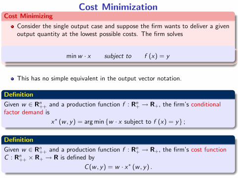
Cost MinimizationCost Minimizing

Consider the single output case and suppose the firm wants to deliver a givenoutput quantity at the lowest possible costs. The firm solves

minw · x subject to f (x) = y

This has no simple equivalent in the output vector notation.

DefinitionGiven w ∈ Rn++ and a production function f : Rn+ → R+, the firm’s conditionalfactor demand is

x∗ (w , y) = argmin {w · x subject to f (x) = y} ;

DefinitionGiven w ∈ Rn++ and a production function f : Rn+ → R+, the firm’s cost functionC : Rn++ × R+ → R is defined by

C (w , y) = w · x∗ (w , y) .

Properties of Cost FunctionsProposition

Given a production function f : Rn+ → R+, the corresponding cost function C (w , y)is concave in w.

Proof.

Question 7c; Problem Set 4. (Hint: use a ‘revealed preferences’argument)

Shephard’s LemmaWrite the Lagrangian

L = w · x − λ [f (x)− y ]

by the Envelope Theorem∂C (w , y)

∂wi=

∂L∂wi

= x∗i (w , y)

Conditional factor demands are downward sloping

Differentiating one more time: ∂C 2(w ,y )∂wi∂wi

=∂x∗i (w ,y )∂wi

≤ 0 where theinequality follows concavity of C (w , y).

Next Class

General equilibrium introduction and notation

Pareto optimality