K.7

Firm-specific risk-neutral distributions: The role of CDS spreads Aramonte, Sirio, Mohammad R. Jahan-Parvar, Samuel Rosen, and John W. Schindler

International Finance Discussion Papers Board of Governors of the Federal Reserve System

Number 1212 August 2017

Please cite paper as: Aramonte, Sirio, Mohammad R. Jahan-Parvar, Samuel Rosen, and John W. Schindler (2017). Firm-specific risk-neutral distributions: The role of CDS spreads. International Finance Discussion Papers 1212. https://doi.org/10.17016/IFDP.2017.1212

Board of Governors of the Federal Reserve System

International Finance Discussion Papers

Number 1212

August 2017

Firm-specific risk-neutral distributions: The role of CDS spreads

Sirio Aramonte, Mohammad R. Jahan-Parvar, Samuel Rosen, and John W. Schindler

NOTE: International Finance Discussion Papers are preliminary materials circulated to stimulate discussion and critical comment. References in publications to International Finance Discussion Papers (other than an acknowledgment that the writer has had access to unpublished material) should be cleared with the author or authors. Recent IFDPs are available on the Web at https://www.federalreserve.gov/econres/ifdp/. This paper can be downloaded without charge from Social Science Research Network electronic library at http://www.sssrn.com.

Firm-specific risk-neutral distributions:

The role of CDS spreads

Sirio Aramonte Mohammad R. Jahan-Parvar Samuel Rosen

John W. Schindler∗

August 9, 2017

Abstract

We propose a method to extract individual firms’ risk-neutral return distributions bycombining options and credit default swaps (CDS). Options provide information aboutthe central part of the distribution, and CDS anchor the left tail. Jointly, optionsand CDS span the intermediate part of the distribution, which is driven by moderate-sized jump risk. We study the returns on a trading strategy that buys (sells) stocksexposed to positive (negative) moderate-sized jump risk unspanned by options or CDSindividually. Controlling for many known factors, this strategy earns a 0.5% premiumper month, highlighting the economic value of combining options and CDS.

Keywords: risk neutral distributions; CDS spreads; cross-section of expected returns

JEL classification: G12; G13; G14

∗Aramonte, Jahan-Parvar, and Schindler are at the Federal Reserve Board. Rosen is at the University ofNorth Carolina at Chapel Hill, Kenan-Flagler Business School. Contact author e-mail and phone number:sirio.aramonte@frb.gov, (202) 912-4301. We would like to thank Jack Bao, Daniel Beltran, Yasser Boualam,Stijn Claessens, Jennifer Conrad, Max Croce, Jesse Davis, Michael Gordy, Pawel Szerszen, and seminarparticipants at the Kenan-Flagler Business School, Federal Reserve Board, University of Warsaw Schoolof Management, CFE 2016 (Seville), IFABS 2016 (Barcelona), JSM 2016 (Chicago), SNDE 2017 (Paris),Georgetown Center for Economic Research Biannual Conference (2017), North American Summer Meetingof the Econometric Society 2017 (St. Louis), and JSM 2017 (Baltimore). This article represents the views ofthe authors, and does not reflect the views of the Board of Governors of the Federal Reserve System or othermembers of its staff.

1

1 Introduction

We propose a new method to extract the risk-neutral distribution of a firm’s expected stock

returns by combining the information contained in option prices and credit default swap

(CDS) spreads. Options characterize the central part of the distribution, and CDS spreads

anchor the left tail. Importantly, the joint use of option prices and CDS spreads allows us to

shed light on the risk-neutral properties of large negative returns that, first, go beyond the

strikes of actively traded options, and second, are not large enough to induce default. The

literature on extracting option-implied return distributions has traditionally focused on broad

equity indexes rather than on individual stocks, although interest in the latter has increased

steadily in recent years. Unlike index options single-stock options tend to trade actively at

strikes concentrated around the current price, hence they provide limited information about

the non-central part of the return distribution.1

We apply our method to a sample of U.S. firms, and we conduct a series of asset pric-

ing tests to document the economic value of extracting risk-neutral distributions using both

option prices and CDS spreads. First, we compare our parametric approach with the es-

tablished non-parametric methodology of Bakshi, Kapadia, and Madan (2003) (henceforth,

BKM). We find that our procedure generally performs as well as BKM, and that it outper-

forms BKM in times of financial market stress. In addition, we focus on the contribution

of CDS by studying a portfolio that buys (sells) stocks for which the options/CDS-implied

skewness is higher (lower) than the option-implied skewness. The portfolio is long (short) on

stocks that are sensitive to moderate-sized positive (negative) jump risk that is not spanned

by options or CDS in isolation. We conduct time-series and cross-sectional asset-pricing tests

to measure the economic significance of this factor, and find that it commands a 0.5% per

month risk premium. We find that our results are robust to a large set of asset pricing fac-

1 A partial list of studies on extracting option-implied distributions for equity indexes includes Bates(1991), Madan and Milne (1994), Rubinstein (1994), Longstaff (1995), Jackwerth and Rubinstein (1996),Aıt-Sahalia and Lo (1998), Bates (2000), Bliss and Panigirtzoglou (2002), Figlewski (2010), Birru andFiglewski (2012), and Andersen, Fusari, and Todorov (2015). Investors are net buyers of index op-tions (Garleanu, Pedersen, and Poteshman, 2009), and index options trade with more out-of-the-money(OTM) strikes than single-stock options since they provide hedge against increases in correlation thatreduce the benefits of diversification (see Driessen, Maenhout, and Vilkov, 2009).

2

tors, stock characteristics, and different assumptions about key inputs of the method, such

as CDS tenor and default thresholds.

Studies of individual-stock risk-neutral distributions often build on the popular method

of Bakshi and Madan (2000) and Bakshi, Kapadia, and Madan (2003) to calculate higher-

order risk-neutral moments from option prices. Examples include Dennis and Mayhew (2002),

Rehman and Vilkov (2012), Bali and Murray (2013), Conrad, Dittmar, and Ghysels (2013),

DeMiguel, Plyakha, Uppal, and Vilkov (2013), and Stilger, Kostakis, and Poon (2017). Some

implementations of this method rely on a potentially small number of options (e.g., Dennis

and Mayhew, 2002, among others) or on interpolated option prices (e.g., An, Ang, Bali, and

Cakici, 2014).

Our proposed method takes advantage of the availability of CDS contracts that were

thinly traded in early 2000s. Since the mid-2000s, both the number and the liquidity of CDS

contracts for U.S. companies have increased significantly. The estimation of risk-neutral

distributions with options and CDS instead of just options can be advantageous for two

reasons. First, CDS contain information about extreme events that liquid options, with

strikes close to the current stock price, do not. This feature is especially valuable since we

can anchor the left tail of the risk-neutral distribution through default probabilities embedded

in CDS spreads. Second, considering CDS and options jointly can provide information that

neither options nor CDS can convey individually. Using CDS and options together provides

information about returns that, in absolute value, are large but not extreme. These returns

are driven by moderate-sized jumps.2 The trade off we face is that we need data for both

options and CDS, which reduces the sample size both in the cross section and in the time

series. In addition, we need to estimate the return threshold where we transition from using

options data to using CDS data.

A number of studies investigate the link between the pricing of options and CDS.

Carr and Wu (2010) develop a model for the joint valuation of options and CDS, where

the default rate is affected by stock volatility. They explicitly model the stock and default

2 Extreme negative jumps force a default, and in the company-specific context of our study, are accountedfor by CDS-implied probabilities of default.

3

dynamics, which entails estimating a relatively large set of parameters. Our approach imposes

a less restrictive structure on the data. Our focus is on three parameters that characterize

a skewed Student-t distribution, which allows us to extract a new distribution for any day

with a sufficient number of option prices.3 Carr and Wu (2011) derive a no-arbitrage relation

between CDS and out of the money (OTM) put options that builds on the existence of

a default corridor for stock prices. They assume that stock prices remain above a certain

threshold before default, and jump below a second threshold upon default. A simple trading

strategy that buys and sells options with strike prices within the default corridor has a

payoff which mimics that of a CDS, thus establishing a no-arbitrage link between the prices

of options and CDS.4

In order for our method to be feasible, stock prices need to be positive just before

default. If stock prices always approach zero before default, bankruptcy would not span a

meaningful set of a firm’s equity return space, and the CDS-implied default probability could

not be used to anchor the left tail of the risk neutral distribution of returns. There is evidence

that debtholders generally have an incentive to strategically force a default before the value

of assets approaches zero, in order to maximize the recovery rate on the debt (see Fan and

Sundaresan, 2000, Carey and Gordy, 2016, and other references in Carr and Wu, 2011).

Our approach of using stock-specific moments to investigate the cross-section of returns

contributes to an active line of research. In particular, our work is close to Stilger, Kostakis,

and Poon (2017), Conrad, Dittmar, and Ghysels (2013) and Rehman and Vilkov (2012).

These studies use the method developed in BKM to calculate risk-neutral higher moments

for individual stocks and document the relation between the extracted moments and future

3 The skewed Student-t distribution is often used to model financial time series, as in Hansen (1994) andPatton (2004).

4 A number of studies focus on the interaction between options or stocks and CDS or corporate bonds.The spreads on bonds and CDS are in theory linked through a no-arbitrage restriction. Among them,Friewald, Wagner, and Zechner (2014) show the CDS spread-term structure contains information aboutthe equity premium. Cao, Yu, and Zhong (2010) document the covariation of CDS spreads and thevolatility risk premium. Cremers, Driessen, and Maenhout (2008) and Cremers, Driessen, Maenhout,and Weinbaum (2008) find that option implied volatilities explain credit spreads. Acharya and Johnson(2007) find that information expressed in CDS spreads is reflected in stock prices with a lag. Ni andPan (2011) study short-sale bans and highlight information flows from CDS to stock prices, while Hanand Zhou (2011) document that the slope of the CDS term structure is related to subsequent returns,in particular for stocks for which arbitrage is more difficult.

4

returns. Our results are in line with the findings of Stilger, Kostakis, and Poon (2017),

Conrad, Dittmar, and Ghysels (2013) and Rehman and Vilkov (2012), but the design of our

study differs from these papers along this important dimension: they are focused on the

direct contribution of risk-neutral higher moments on future return predictability, while we

are focused on the differential between options/CDS-implied and option-implied skewness.

The voluminous literature on index options has highlighted the importance of higher

order moments for asset pricing since the mid-2000s. The literature on risk-neutral skewness

is predated by studies on skewness extracted from historical returns. Harvey and Siddique

(2000) find that systematic skewness helps explain the cross section of returns. Account-

ing for skewness is also important to identify the sign of the risk-return relation, see Fe-

unou, Jahan-Parvar, and Tedongap (2013). Amaya, Christoffersen, Jacobs, and Vasquez

(2015) find that realized skewness generates cross-sectional predictability in stock returns.

Recently, Colacito, Ghysels, Meng, and Siwasarit (2016) investigate the effect of skewness

in firm-level and macroeconomic fundamentals on stock returns. As documented by Kim

and White (2004), measuring historical higher moments is difficult. Feunou, Jahan-Parvar,

and Tedongap (2016), examine alternative parametric structures for skewness models, and

Neuberger (2012) develops a realized estimator for skewness based on high-frequency data.

Ghysels, Plazzi, and Valkanov (2016) use quantile-based measures of skewness to overcome

data constraints in emerging markets. Khozan, Neuberger, and Schneider (2013) analyze

skewness risk premium with a trading strategy that replicates a skew swap whose payoff is

the difference between option-implied skewness and realized skewness. They find that vari-

ance risk and skewness risk are closely related, in that trading strategies which load on one

of the two and hedge the other do not earn a risk premium.

The rest of the paper is organized as follows. Section 2 describes the data used in

our study. In Section 3 we present the method for extracting the options/CDS-implied

risk-neutral distributions. Section 4 discusses our empirical investigation and findings, and

Section 5 concludes.

5

2 Data

Our sample encompasses option prices, CDS spreads, and company stock returns from Jan-

uary 2006 to December 2015. We choose to focus on this period due to CDS data availability

and reliability. Options and interest rate data are from OptionMetrics through Wharton Re-

search Data Services (WRDS). We collect American options (with an “A” exercise style flag)

written on individual common stocks (CRSP share codes 10 and 11) that trade on AMEX,

NASDAQ, or NYSE (CRSP exchange codes 1, 2, and 3). As is customary with options data,

we apply a series of filters to discard thinly-traded options and likely data errors. We keep

observations with positive volume, positive bid and ask prices, and an ask price higher than

the bid price. Following Santa-Clara and Saretto (2009), we drop options with a bid-ask

spread smaller than the minimum tick (0.05 if the ask is less than 3, and 0.1 if the bid is

more than or equal to 3). Finally, we discard options with missing observations for implied

volatility.

The CDS data are from Markit. They include the term structure of CDS spreads

between 6 months and 30 years, in addition to recovery rates and restructuring clauses.

Moreover, Markit provides information on the reference obligation, including seniority and

country of domicile for the issuer. We focus on U.S. Dollar-denominated CDS contracts

on senior unsecured obligations issued by U.S.-based entities. We consider CDS spreads

pertaining to contracts with an XR restructuring clause. Restructuring clauses determine

what credit events trigger the payout of the CDS, and the XR clause excludes all debt

restructuring as trigger events.

The bankruptcy data are from CapitalIQ, and we consider bankruptcy filings (event

code 89) between 1990 and 2015. Some firms experience multiple bankruptcies, in which case

we only include the first one, unless there is a five-year gap between bankruptcies.

We obtain stock returns from the Center for Research on Security Prices (CRSP) and

balance-sheet items through Compustat. We manually match companies in Markit and

CRSP by name, and we merge Compustat and OptionMetrics using the the lpermno and

cusip variables.

6

On any given day, we select the cross section of options with maturity closest to 90

calendar days, as long as the maturity is between 15 and 180 days. We require that the CDS

spread and at least five option observations are available for each company/day combination.

Table 1 shows selected summary statistics for the resulting 275 companies as of 2006. These

companies are large, with median book assets equal to about $13 billion. The average of

book assets is about $63 billion, which indicates the presence of several very large companies.

The remaining summary statistics are financial and balance sheet ratios, all scaled by book

assets at the end of 2005, and show that there is substantial heterogeneity in our sample

along several dimensions, including cash flows, sales, investment, research and development

expense, and stock and debt issuance.

Although the companies in our sample are typically large, the strike coverage and traded

volume of options written on their stocks remain pervasively low. The summary statistics

in Table 2 highlight the differences in the availability of strike prices between options on the

S&P 500 index and on the companies we study. We apply the filters described earlier in this

section to both index and stock options, and we define a call (put) option as OTM if the

strike is above (below) the stock price. A put option is considered deep OTM if its strike

price is less than 80% of the stock price.

The top panel of Table 2 shows that, for the S&P 500, OTM options trade more often

than their in-the-money (ITM) counterparts, with the average number of OTM options equal

to 14.69 (puts) and 12.02 (calls) and the corresponding averages for ITM options equal to

4.29 (puts) and 5.40 (calls). The average daily number of deep OTM put options is about 8,

or roughly half the average number of OTM put options. Turning to individual-stock options

in the bottom panel, the average number of option prices is considerably lower across both

moneyess and call/put types, and there is little difference in availability between ITM and

OTM options. The average number of deep OTM put options is roughly 2, and the median

equals 1.

Additionally, the two rightmost columns of Table 2 report summary statistics for op-

tion volume along moneyness and call/put types. We observe the same patterns that we

discussed for the number of available options. Trading volumes are one order of magnitude

7

smaller for individual-stock options compared to index options, and the difference is even

more pronounced for OTM puts. Overall, the evidence in Table 2 point to the value of incor-

porating left-tail information from CDS spreads when studying the risk-neutral distributions

of individual stocks.

3 Options/CDS-implied return distributions

Our method for estimating risk-neutral distributions is based on three ingredients: option

prices, CDS spreads, and a default threshold. Option prices provide information about the

central part of the distribution, while CDS spreads anchor the left tail. The probability of

default embedded in the CDS contract is the cumulative density up to the default threshold.

The default threshold pins the transition point between options- and CDS-based information.

Figure 1 illustrates graphically how options and CDS information are combined to yield the

risk-neutral distribution.

As highlighted in the previous section, options with a strike price close to the default

threshold are very thinly traded. On the other hand, CDS contracts, especially since the

mid-2000s, have an active market. By definition, CDS with an XR restructuring clause pay

upon default, which means that their “strike price” is at the default threshold. Table 3

provides a hypothetical example of the typical availability of CDS and options with different

strikes, and of the informativeness of CDS and options with different strikes about default

risk. The current stock prices is $100 and default happens when the stock price drops to $20.

Options with strike price close to the underlying price (strikes equal to $110 and $90) are

actively traded but they are not informative about the probability of default. The reason is

that these options speak to the probability of moderate price changes (±10%), however they

do not provide information about significant price drops that could push the company into

default. Single-name options with a strike price significantly below the current stock price

and close to the default threshold ($20, in this case) rarely trade. Thus, while potentially

informative, they are not readily available. CDS, on the other hand, have an implicit strike

price that is equal to the default threshold and they are actively traded, hence they meet

both requirements.

8

For each stock/day pair, we estimate the parameters of a skewed Student-t distribution

(Hansen, 1994 and Patton, 2004) by minimizing the squared deviations between the empirical

and parametric cumulative probability functions measured at the default threshold and at the

option strike prices. The empirical cumulative probability at the default threshold is equal

to the CDS-implied default probability, while the option-implied probabilities are computed

using standard methods that build on the link between the call pricing function and the

probability distribution highlighted in Breeden and Litzenberger (1978).

The probability density function of the skewed Student-t distribution is given by:

f(zj) =

bc

(1 + 1

η−2

(bzj+a1−λ

)2)−(η+1)/2

if zj < −a/b

bc

(1 + 1

η−2

(bzj+a1+λ

)2)−(η+1)/2

if zj ≥ −a/b(1)

where λ (|λ| < 1) is the shape parameter, η (2 < η < ∞) are the degrees of freedom, and

zj = rj−rfσj is the standardized return for company j with expected return rf and volatility

σj. Setting the expected return equal to the risk-free rate rf for all companies enforces the

martingale restriction under the risk-neutral measure.

The skewness sk and kurtosis ku of the skewed Student-t distribution are defined as

follows (Feunou, Jahan-Parvar, and Tedongap, 2016):sk = (m3 − 3am2 + 2a3)/b3

ku = (m4 − 4am3 + 6a2m2 − 3a4)/b4

(2)

where a = 4λcη−2η−1

, b =√

1 + 3λ2 − a2, c = Γ((η+1)/2)

Γ(η/2)√π(η−2)

, m2 = 1 + 3λ2, m3 = 16cλ(1 +

λ2) (η−2)2

(η−1)(η−3)(for η > 3), and m4 = 3η−2

η−4(1 + 10λ2 + 5λ4) (for η > 4).

Our goal is recovering risk-neutral distributions of three-month ahead expected returns.

Options with a maturity of exactly three months are generally not available. As a result,

for each day and for each company we choose the cross section of options with maturity

closest to three months, as long as the maturity is between 15 and 180 days. Note that

the risk-neutral cumulative density function (CDF) of returns is the first derivative of the

European price function, but exchange-traded options on individual companies are Ameri-

9

can options. We convert American prices into their European equivalent with three-month

maturity by calculating the Black-Scholes price based on the implied volatility provided by

OptionMetrics, which is computed according to a Cox, Ross, and Rubinstein (1979) bino-

mial tree and does not incorporate the early exercise premium. In that, we follow Broadie,

Chernov, and Johannes (2007).

3.1 Option-implied return probabilities

A number of contributions to the literature on option-implied distributions exploit the equal-

ity of the density to the scaled second derivative of the call price function with respect to the

strike price (Breeden and Litzenberger, 1978). Other studies use binomial trees (Rubinstein,

1994, Jackwerth and Rubinstein, 1996) and kernel regressions (Aıt-Sahalia and Lo, 1998).

Once away from at-the-money strikes, there are fewer options and those that are avail-

able are less liquid. Existing studies often obtain a denser set of option prices by interpo-

lating/extrapolating the cross-section of implied volatilities (relative to strike prices) and

inverting the set of traded and interpolated implied volatilities back to prices. The interpo-

lation is often based on non-parametric techniques, like parabolic functions (Shimko, 1993)

or cubic and quartic splines. The shape of the tails of the implied distributions depends

crucially on the extrapolation method and on the leverage exerted by the implied volatilities

at the extremes of the set of traded strikes. The literature has proposed to model the tails

parametrically in order to limit this sensitivity (Shimko, 1993, Figlewski, 2010).

Our method for extracting the risk-neutral distribution of stock returns builds on the

established literature that uses the first derivatives of the European call pricing function,

relative to the strike price, to approximate the CDF of stock returns. We follow Figlewski

(2010) when calculating the option-implied cumulative probabilities at the traded strikes, and

we compute the cumulative probability at the default threshold using CDS spreads and the

technique discussed in Section 3.3. We then estimate the parameters of a skewed Student-t

distribution by minimizing the squared deviations between the skewed Student-t CDF and

the cumulative probabilities extracted from options and CDS.

10

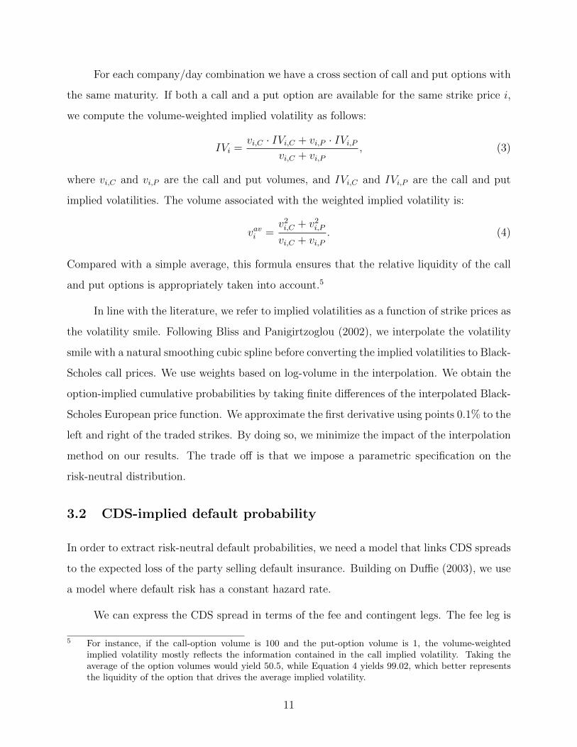
For each company/day combination we have a cross section of call and put options with

the same maturity. If both a call and a put option are available for the same strike price i,

we compute the volume-weighted implied volatility as follows:

IVi =vi,C · IVi,C + vi,P · IVi,P

vi,C + vi,P, (3)

where vi,C and vi,P are the call and put volumes, and IVi,C and IVi,P are the call and put

implied volatilities. The volume associated with the weighted implied volatility is:

vavi =v2i,C + v2

i,P

vi,C + vi,P. (4)

Compared with a simple average, this formula ensures that the relative liquidity of the call

and put options is appropriately taken into account.5

In line with the literature, we refer to implied volatilities as a function of strike prices as

the volatility smile. Following Bliss and Panigirtzoglou (2002), we interpolate the volatility

smile with a natural smoothing cubic spline before converting the implied volatilities to Black-

Scholes call prices. We use weights based on log-volume in the interpolation. We obtain the

option-implied cumulative probabilities by taking finite differences of the interpolated Black-

Scholes European price function. We approximate the first derivative using points 0.1% to the

left and right of the traded strikes. By doing so, we minimize the impact of the interpolation

method on our results. The trade off is that we impose a parametric specification on the

risk-neutral distribution.

3.2 CDS-implied default probability

In order to extract risk-neutral default probabilities, we need a model that links CDS spreads

to the expected loss of the party selling default insurance. Building on Duffie (2003), we use

a model where default risk has a constant hazard rate.

We can express the CDS spread in terms of the fee and contingent legs. The fee leg is

5 For instance, if the call-option volume is 100 and the put-option volume is 1, the volume-weightedimplied volatility mostly reflects the information contained in the call implied volatility. Taking theaverage of the option volumes would yield 50.5, while Equation 4 yields 99.02, which better representsthe liquidity of the option that drives the average implied volatility.

11

the expected value of the payments received by the protection seller. The contingent leg is the

expected value of the losses incurred by the protection seller. As detailed below, we observe

the CDS spread and all the variables that determine the value of the fee and contingent legs,

with the exception of the hazard rate. This rate is computed numerically by equating the

CDS spread to the ratio of the contingent and fee legs.

The value of the fee leg of a CDS with maturity TN and payment dates {Ti}Ni=1 can be

expressed as a function of the spread, s, the hazard rate, λ, the risk-free discount rate, rfi ,

and of the time between Ti−1 and Ti (∆i):6

Vf (λ, TN) = s · ΣNi=1

{∆ie

−λTi−1

[e−λ∆i +

(1− e−λ∆i

) λ−1 − e−λ∆i (∆i + λ−1)

1− e−λ∆i

]e−r

fi Ti

}= s · ΣN

i=1

{∆ie

−λTi−1[e−λ∆i + λ−1 − e−λ∆i

(∆i + λ−1

)]e−r

fi Ti}

(5)

The first exponential in curly brackets is the survival probability up to time Ti−1. The

expression in square brackets gives the expected fee between time Ti−1 and time Ti: the

firm survives one more period, in which case the full fee is collected; or the firm defaults,

so that only the accrued premium is collected. The accrued premium is given by the spread

times the expected time of default, conditional on default taking place in the interval ∆i, as

captured by the fraction next to the closing square bracket. The last term in the formula is

the discount factor.

The expected time of default, conditional on default taking place in the interval ∆i, is:

E [x|0 < x ≤ ∆i] =

∫ ∆i

0

xf(x)∫ ∆i

0f(x)dx

dx =

∫ ∆i

0

xλe−λx

1− e−λ∆idx

=1

1− e−λ∆iλ

[−xe−λx

λ

∣∣∣∣∆i

0

+−e−λx

λ2

∣∣∣∣∆i

0

]

=λ−1 − e−λ∆i(∆i + λ−1)

1− e−λ∆i(6)

6 Our specification builds on Duffie (2003) and JPMorgan (2001). See the ISDA “Standard North Amer-ican Corporate CDS Contract Specification” for details on the pricing and timing conventions for cor-porate CDS.

12

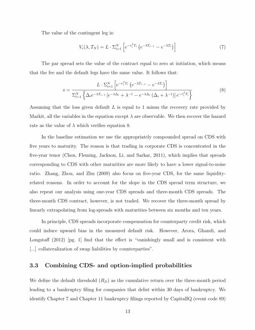
The value of the contingent leg is:

Vc(λ, TN) = L · ΣNi=1

[e−r

fi Ti(e−λTi−1 − e−λTi

)](7)

The par spread sets the value of the contract equal to zero at initiation, which means

that the fee and the default legs have the same value. It follows that:

s =L · ΣN

i=1

[e−r

fi Ti(e−λTi−1 − e−λTi

)]ΣNi=1

{∆ie−λTi−1 [e−λ∆i + λ−1 − e−λ∆i (∆i + λ−1)] e−r

fi Ti

} (8)

Assuming that the loss given default L is equal to 1 minus the recovery rate provided by

Markit, all the variables in the equation except λ are observable. We then recover the hazard

rate as the value of λ which verifies equation 8.

In the baseline estimation we use the appropriately compounded spread on CDS with

five years to maturity. The reason is that trading in corporate CDS is concentrated in the

five-year tenor (Chen, Fleming, Jackson, Li, and Sarkar, 2011), which implies that spreads

corresponding to CDS with other maturities are more likely to have a lower signal-to-noise

ratio. Zhang, Zhou, and Zhu (2009) also focus on five-year CDS, for the same liquidity-

related reasons. In order to account for the slope in the CDS spread term structure, we

also repeat our analysis using one-year CDS spreads and three-month CDS spreads. The

three-month CDS contract, however, is not traded. We recover the three-month spread by

linearly extrapolating from log-spreads with maturities between six months and ten years.

In principle, CDS spreads incorporate compensation for counterparty credit risk, which

could induce upward bias in the measured default risk. However, Arora, Ghandi, and

Longstaff (2012) [pg. 1] find that the effect is “vanishingly small and is consistent with

[...] collateralization of swap liabilities by counterparties”.

3.3 Combining CDS- and option-implied probabilities

We define the default threshold (RD) as the cumulative return over the three-month period

leading to a bankruptcy filing for companies that delist within 30 days of bankruptcy. We

identify Chapter 7 and Chapter 11 bankruptcy filings reported by CapitalIQ (event code 89)

13

between 1990 and 2015, excluding companies with a market capitalization below $100 million

one year before the bankruptcy filing. For companies that default multiple times, only the

first instance is included unless the bankruptcies are at least five years apart.

We first compute four different default thresholds by double sorting companies on the

basis of market capitalization and leverage one year and one quarter before the bankruptcy

filing. The market capitalization breakpoint is $1 billion, and the leverage breakpoint is the

bankruptcy-sample median. The rationale for using a five-quarter gap is that we need one

quarter to calculate the default threshold, and we lag the firm characteristics by one year to

limit the impact of the looming bankruptcy on market capitalization and leverage.

For robustness, we also consider three additional default thresholds. First, we take

the average of the thresholds obtained by double sorting companies on the basis of size and

leverage. Second, we use a threshold equal to 120% of the this average. Third, we set the

threshold to 80% of the average. Evaluating the robustness to different default thresholds

is also informative about the robustness of our results to different recovery rates, since both

changing the threshold and changing the recovery rate ultimately alter the default probability

extracted from CDS spreads.

Panel A in Table 4 reports the four default thresholds estimated by double sorting

companies on size and leverage. The thresholds are expressed in both log and arithmetic

returns. Large companies with low leverage experience noticeably more negative returns

than small companies with high leverage in the run up to bankruptcy (-0.90 vs -0.70).

As shown in Panel B of Table 4, the mean of the four log-return thresholds equals -1.85,

corresponding to -0.84 in arithmetic returns. The 120% and 80% of the mean are -2.23 and

-1.48, respectively. The corresponding arithmetic returns are -0.89 and -0.77.

Sections 3.1 and 3.2 describe how we calculate the option-implied cumulative return

probabilities and the CDS-implied default probability. Now we discuss how to combine these

probabilities to estimate a parametric risk-neutral distribution of returns. We assume that,

under the risk-neutral measure, returns follow a skewed Student-t distribution. Hansen (1994)

and Patton (2004) study financial applications of the skewed Student-t distribution under

14

the physical measure.

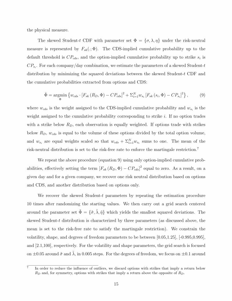
The skewed Student-t CDF with parameter set Φ = {σ, λ, η} under the risk-neutral

measure is represented by Fsk(.; Φ). The CDS-implied cumulative probability up to the

default threshold is CPcds, and the option-implied cumulative probability up to strike si is

CPsi . For each company/day combination, we estimate the parameters of a skewed Student-t

distribution by minimizing the squared deviations between the skewed Student-t CDF and

the cumulative probabilities extracted from options and CDS:

Φ = argminΦ

{wcds · [Fsk (RD,Φ)− CPcds]2 + ΣN

i=1wsi [Fsk (si,Φ)− CPsi ]2} , (9)

where wcds is the weight assigned to the CDS-implied cumulative probability and wsi is the

weight assigned to the cumulative probability corresponding to strike i. If no option trades

with a strike below RD, each observation is equally weighted. If options trade with strikes

below RD, wcds is equal to the volume of these options divided by the total option volume,

and wsi are equal weights scaled so that wcds + ΣNi=1wsi sums to one. The mean of the

risk-neutral distribution is set to the risk-free rate to enforce the martingale restriction.7

We repeat the above procedure (equation 9) using only option-implied cumulative prob-

abilities, effectively setting the term [Fsk (RD,Φ)− CPcds]2 equal to zero. As a result, on a

given day and for a given company, we recover one risk neutral distribution based on options

and CDS, and another distribution based on options only.

We recover the skewed Student-t parameters by repeating the estimation procedure

10 times after randomizing the starting values. We then carry out a grid search centered

around the parameter set Φ = {σ, λ, η} which yields the smallest squared deviations. The

skewed Student-t distribution is characterized by three parameters (as discussed above, the

mean is set to the risk-free rate to satisfy the martingale restriction). We constrain the

volatility, shape, and degrees of freedom parameters to be between [0.05,1.25], [-0.995,0.995],

and [2.1,100], respectively. For the volatility and shape parameters, the grid search is focused

on ±0.05 around σ and λ, in 0.005 steps. For the degrees of freedom, we focus on ±0.1 around

7 In order to reduce the influence of outliers, we discard options with strikes that imply a return belowRD and, for symmetry, options with strikes that imply a return above the opposite of RD.

15

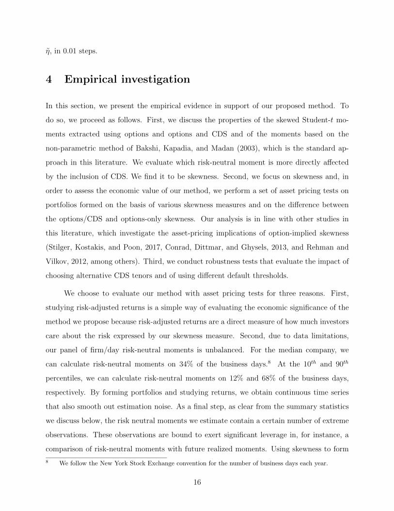
η, in 0.01 steps.

4 Empirical investigation

In this section, we present the empirical evidence in support of our proposed method. To

do so, we proceed as follows. First, we discuss the properties of the skewed Student-t mo-

ments extracted using options and options and CDS and of the moments based on the

non-parametric method of Bakshi, Kapadia, and Madan (2003), which is the standard ap-

proach in this literature. We evaluate which risk-neutral moment is more directly affected

by the inclusion of CDS. We find it to be skewness. Second, we focus on skewness and, in

order to assess the economic value of our method, we perform a set of asset pricing tests on

portfolios formed on the basis of various skewness measures and on the difference between

the options/CDS and options-only skewness. Our analysis is in line with other studies in

this literature, which investigate the asset-pricing implications of option-implied skewness

(Stilger, Kostakis, and Poon, 2017, Conrad, Dittmar, and Ghysels, 2013, and Rehman and

Vilkov, 2012, among others). Third, we conduct robustness tests that evaluate the impact of

choosing alternative CDS tenors and of using different default thresholds.

We choose to evaluate our method with asset pricing tests for three reasons. First,

studying risk-adjusted returns is a simple way of evaluating the economic significance of the

method we propose because risk-adjusted returns are a direct measure of how much investors

care about the risk expressed by our skewness measure. Second, due to data limitations,

our panel of firm/day risk-neutral moments is unbalanced. For the median company, we

can calculate risk-neutral moments on 34% of the business days.8 At the 10th and 90th

percentiles, we can calculate risk-neutral moments on 12% and 68% of the business days,

respectively. By forming portfolios and studying returns, we obtain continuous time series

that also smooth out estimation noise. As a final step, as clear from the summary statistics

we discuss below, the risk neutral moments we estimate contain a certain number of extreme

observations. These observations are bound to exert significant leverage in, for instance, a

comparison of risk-neutral moments with future realized moments. Using skewness to form

8 We follow the New York Stock Exchange convention for the number of business days each year.

16

stock portfolios and studying the returns of these portfolios avoids econometric issues, since

stock returns are well behaved. We could discard extreme observations. However they could

contain economic information about investment opportunities – our sample includes the 2008

financial crisis and the ensuing high-volatility years. In portfolio-based tests, we let these

observations inform portfolio formation without worrying about econometric issues.

We conduct asset-pricing tests using monthly returns. We assign companies to portfo-

lios based on moments as of the end of the previous month. In order to smooth potential

estimation noise, while also retaining timely information, we average the moments over the

last three days of the month (Stilger, Kostakis, and Poon, 2017 also use end-of-month mo-

ments).

Including CDS in the estimation of the risk-neutral distributions does not necessarily

lead to very large changes in the shape of the density function. Figure 2 provides an example.

This figure plots the options-only and options/CDS risk-neutral densities for Citigroup Inc.

on July 20, 2009. As is clear from the figure, the inclusion of CDS has a noticeable effect on

the shape of the risk-neutral distribution.

4.1 Risk-neutral moments and the inclusion of CDS

In order to understand which moment of the risk-neutral distributions is primarily affected

by the inclusion of CDS, we compare the moments of options/CDS and options-only risk-

neutral distributions. We expect CDS to affect kurtosis and skewness more than volatility,

since the latter is well characterized by options with strike prices around the current stock

price. Kurtosis, on the other hand, measures the thickness of tails, which is directly linked

to the default probability expressed by CDS spreads. Skewness measures the shape of a

distribution, which is influenced by both the central part and the tails.

For each moment (volatility, skewness, and kurtosis), we construct the absolute differ-

ence between the options/CDS moment and the options-only moment, scaled by the absolute

value of the options-only moment (|momopt/CDS−momopt|

|momopt| ). Panel A of Table 5 shows the aver-

age and upper percentiles of the absolute relative differences’ distribution. It is immediately

17

clear that, first, the moment most affected by the inclusion of CDS is skewness, followed

by kurtosis. Second, we observe that meaningful differences between the options/CDS and

options-only skewness are concentrated above the 75th percentile.

The estimation of risk-neutral distributions with options and CDS instead of just op-

tions can be advantageous for two reasons. First, CDS contain information about extreme

events that liquid options, with strikes close to the current stock price, do not. This informa-

tion directly affects the estimation of kurtosis. Second, considering CDS and options jointly

can provide information that neither options nor CDS can convey individually. Figure 1

illustrates that the default probability implied by CDS spreads pins down the far left tail,

and that options are informative about the central part of the distribution. The intermediate

part of the distribution is not spanned by either CDS or options in isolation. However, using

CDS and options together provides information about returns that, in absolute value, are

large but not extreme. This information affects the estimation of skewness.

The information about probabilities of default embedded in CDS spreads directly affect

kurtosis. This information indirectly affect skewness, and only in conjunction with options

data. As a result, we expect CDS spreads to explain the difference between options/CDS and

option-only kurtosis to a larger extent than they explain the difference between options/CDS

and options-only skewness. We expect this to be the case even though skewness is the

moment that changes by inclusion of CDS in recovering of risk neutral distributions. In

Panel B of Table 5, we report the results of regressing skopt/CDS − skopt or kuopt/CDS − kuopton 5-year CDS log spreads. The regression results point to stronger direct influence of CDS

on kurtosis than on skewness, even though skewness is more affected than kurtosis by the

inclusion of CDS in the procedure for extracting risk-neutral densities, as shown in Panel A.

When focusing on non-zero differences, the slope parameter for CDS spreads is statistically

significant only for kurtosis. This coefficient becomes statistically significant for skewness only

when the differences become increasingly larger. The magnitude and statistical significance

of the slope coefficient, as well as the R2s, are always larger for kurtosis than for skewness.

Considering the evidence presented in Panels A and B, one can easily conclude that

joint consideration of options and CDS influences skewness more than kurtosis. As a result,

18

in the remainder of the paper we focus on skewness. Moreover, Stilger, Kostakis, and Poon

(2017), Conrad, Dittmar, and Ghysels (2013), and Rehman and Vilkov (2012) find that firm-

specific risk-neutral skewness is priced in the cross-section of stock returns, which makes

skewness of particular interest to the finance community.

We interpret our results in terms of moderate-jump risk that is unspanned by options or

CDS individually. We provide empirical evidence to this effect in Section 4.3. An active line

of research in financial economics studies the link between conditional skewness and jumps.

Recent examples include Patton and Sheppard (2015), Bandi and Reno (2016), and Feunou,

Jahan-Parvar, and Okou (Forthcoming). These studies focus on aggregate stock market

returns, and as such, investigate both large and medium-scale jumps. In our framework, we

consider the link between medium-scale jumps and skewness, since the risk of large jumps

that can push a company into bankruptcy is captured by CDS spreads.

4.2 Evaluating measures of risk-neutral skewness

In Panel A of Table 6, we report summary statistics for skewness measures extracted from

options and CDS, from options only, and for the difference between the two. These moments

are recovered using our parametric method. In Panel B, we compare the non-parametric

skewness measure of Bakshi, Kapadia, and Madan (2003) (henceforth, BKM), as implemented

by Conrad, Dittmar, and Ghysels (2013), to our options/CDS and options-only measures.

As shown in Panel A, differences between the options/CDS and options-only measures are

concentrated in the tails. Panel B highlights that the BKM skewness measure is generally

comparable to ours. However, there are noticeable differences between BKM’s measure and

ours, especially in the tails.

In what follows we compare the BKM, options-only, and options/CDS skewness using

the returns on portfolios formed on each measure. Each portfolio is long (short) stocks in the

top (bottom) 25% of the skewness distribution at the end of the previous month. Figure 3

shows the cumulative returns on the three skewness portfolios and the UMD momentum port-

folio of Carhart (1997). The returns on the options/CDS (SKEWopt/CDS) and options-only

(SKEWopt) portfolios are similar, but not identical. The BKM portfolio (SKEWBKM) tracks

19

the two other skewness portfolios closely until early 2009. However, the portfolios based on

our parametric skewness measures outperform the non-parametric BKM portfolio through

2009. This performance gap only starts to close in late 2014. Since the options/CDS and

options-only portfolios have similar cumulative returns, the outperformance of the portfolios

based on our method relative to BKM is not driven by the inclusion of CDS. The sub-

stantive difference seems to lie with our use of a parametric method to recover risk-neutral

distributions.

We test the relationship between the BKM and options/CDS portfolio returns formally,

by regressing options/CDS-portfolio returns on BKM-portfolio returns and a set of additional

risk factors, including the five Fama and French (2015) factors, changes in the spread of the

CDS-index CDX High Yield (to capture economy-wide default risk), and a factor-mimicking

portfolio for changes in the implied volatility index (VIX). Using a factor-mimicking portfolio

for VIX changes allows us to interpret the intercepts of the time-series regressions as risk-

adjusted average returns.9 We report our findings in Panel A of Table 7. The coefficients

on the BKM portfolio are statistically significant both in the full sample and in the 2008-

2011 sample, which focuses on the global financial crisis and its immediate aftermath. The

statistical significance of the estimated intercept in the 2008-2011 period implies that the

returns on the options/CDS factor are not fully explained by the other factors included in

the regression model. This result is consistent with the evidence presented in Figure 3, which

shows that the options/CDS factor outperforms the BKM factor precisely in the aftermath

the 2008 financial crisis.

A possible reason for the options/CDS and options-only portfolios outperforming the

BKM portfolio throughout 2009 is that the parametric nature of our method enables us to

more efficiently extract information about future investment opportunities. Indeed, early

9 The factor mimicking portfolio is built using stocks for which we can calculate the volatility spreads ofBali and Hovakimian (2009) and the implied-volatility smirk of Xing, Zhang, and Zhao (2010). Thesestocks are also used to replicate the 25 size/book-to-market portfolios of Fama and French (1993) thatwe use in the cross-sectional asset pricing tests discussed in Section 4.4. We regress monthly stockreturns in excess of the risk-free rate on the three Fama and French (1993) factors plus momentum, andchanges in VIX, changes in VIX squared, and the variance risk premium of Bollerslev, Tauchen, andZhou (2009) over the 2006-2015 time period. The equally-weighted replicating portfolio is long (short)stocks whose factor loadings on VIX changes are in the top (bottom) 25% of the distribution.

20

2009 is when the stock market bottomed out and a sustained recovery commenced. We can

make an interesting comparison of the returns on the options/CDS and options-only portfolios

with the momentum strategy. As discussed by Barroso and Santa-Clara (2015) and Daniel

and Moskowitz (2016), and as shown in Figure 3, the momentum strategy experienced very

poor returns through 2009. Momentum is a backward-looking strategy that performs poorly

when confronted with sharp changes in the business cycle. At the end of a long recession, like

the one that began in December 2007, the momentum strategy would buy stocks that have

performed well (e.g., low-beta stocks) and sell stocks that have performed poorly (e.g., high-

beta stocks). After a sharp change in the business cycle and in the stock market trend, and

for a length of time that depends on the portfolio-formation period, the momentum strategy

would keep buying (selling) stocks that have done relatively well during the recession but

that will perform relatively poorly with the new upward trend (e.g., the strategy would keep

buying low-beta stocks and selling high-beta stocks).

To the extent that our method extracts information about future investment opportu-

nities efficiently, the returns on the portfolios based on the options/CDS and options-only

skewness measures should be negatively correlated with the returns on the momentum strat-

egy during the year 2009. The top panel in Figure 4 shows that such is the case. The returns

on the options/CDS portfolio are clearly negatively correlated with momentum returns, and

the most negative momentum return (April 2009) corresponds to the largest return on the

options/CDS portfolio. The bottom panel of this figure shows that the correlation between

momentum and BKM skewness portfolio returns is far less pronounced.

We formally test the relationship between the momentum strategy and options/CDS

or the BKM skewness, by regressing momentum portfolio returns on options/CDS or the

BKM portfolio returns, along with the same risk factors used to evaluate the relationship

between the two skewness portfolio returns. Panel B of Table 7 reports these results. As

expected, the estimated slope parameters for options/CDS portfolio returns are statistically

different from zero and negative-valued in the full sample and in the 2008-2011 sub-sample.

Estimated intercepts for the regression models that include options/CDS portfolio returns

as a factor are statistically indistinguishable from zero both for the full sample and the

21

2008-2011 sub-sample. Conversely, the estimated slope coefficients for the BKM portfolio

returns are statistically insignificant regardless of the sample used. The estimated intercept

parameter for the model containing the BKM portfolio returns as an independent variable

is statistically different from zero at the 10% significance level only in the 2008-2011 sub-

sample. These results support the visual evidence presented in Figure 3. The BKM portfolio

returns are not significantly correlated with the momentum factor. Moreover, particularly

during the global financial crisis and its immediate aftermath, BKM portfolio returns and

other risk factors used in this testing exercise do not fully span the momentum factor. On

the other hand, the momentum factor is fully spanned, regardless of the sample used, by the

options/CDS portfolio returns and the additional risk factors.

Since the philosophy behind the construction of the momentum and options/CDS skew-

ness portfolios are completely different, these findings cannot be attributed to data mining –

a serious concern in recent studies of factors aiming to explain the cross-sectional variations

of stock returns (see Harvey, Liu, and Zhu, 2016). We discuss this issue in greater detail after

presenting our time-series and cross-sectional evidence in support of our proposed method.

4.3 Benefits of including CDS: Rationale for asset-pricing tests

Thus far we have conducted a comparison of different skewness measures using the returns

on portfolios based on each measure. We have shown that our parametric approach compares

well to the established BKM method, and it outperforms BKM during times of high volatility.

We now turn to evaluating the economic significance of the contribution of CDS to the

computation of risk-neutral skewness.

As shown in Figure 3, the cumulative returns on the SKEWopt/CDS and SKEWopt portfo-

lios are fairly close, with SKEWopt/CDS outperforming SKEWopt only slightly over the sample

period. In order to evaluate the economic significance of the CDS contribution, however, one

should not focus on the difference between SKEWopt/CDS and SKEWopt. Rather, the focus

should be on a portfolio that explicitly loads on the differences between the options/CDS and

options-only skewness measures. By doing so, the dynamics of portfolio returns are driven

specifically by skewness differences that arise from the inclusion of CDS. In tests that use

22

portfolios based on skewness levels, the contribution of CDS is likely to be overshadowed by

broad skewness-related dynamics.

We investigate whether differences between the options/CDS and options-only skewness

give rise to a priced factor in the cross-section of stock returns. The battery of tests that we

conduct revolve around a factor-mimicking portfolio that buys and sells stocks on the basis of

differences between options/CDS and options-only risk-neutral skewness (henceforth, the DS

factor). This factor is defined as the returns on a portfolio that buys (sells) the stocks in the

top (bottom) 25% of the distribution of options/CDS and options-only skewness differences

in month t-1. In unreported results, we define the DS factor using a top/bottom 10% cutoff,

with similar conclusions. For each company, we discard the return on the first day of the

month to avoid possible issues with non-synchronous trading between options, CDS, and

stocks.

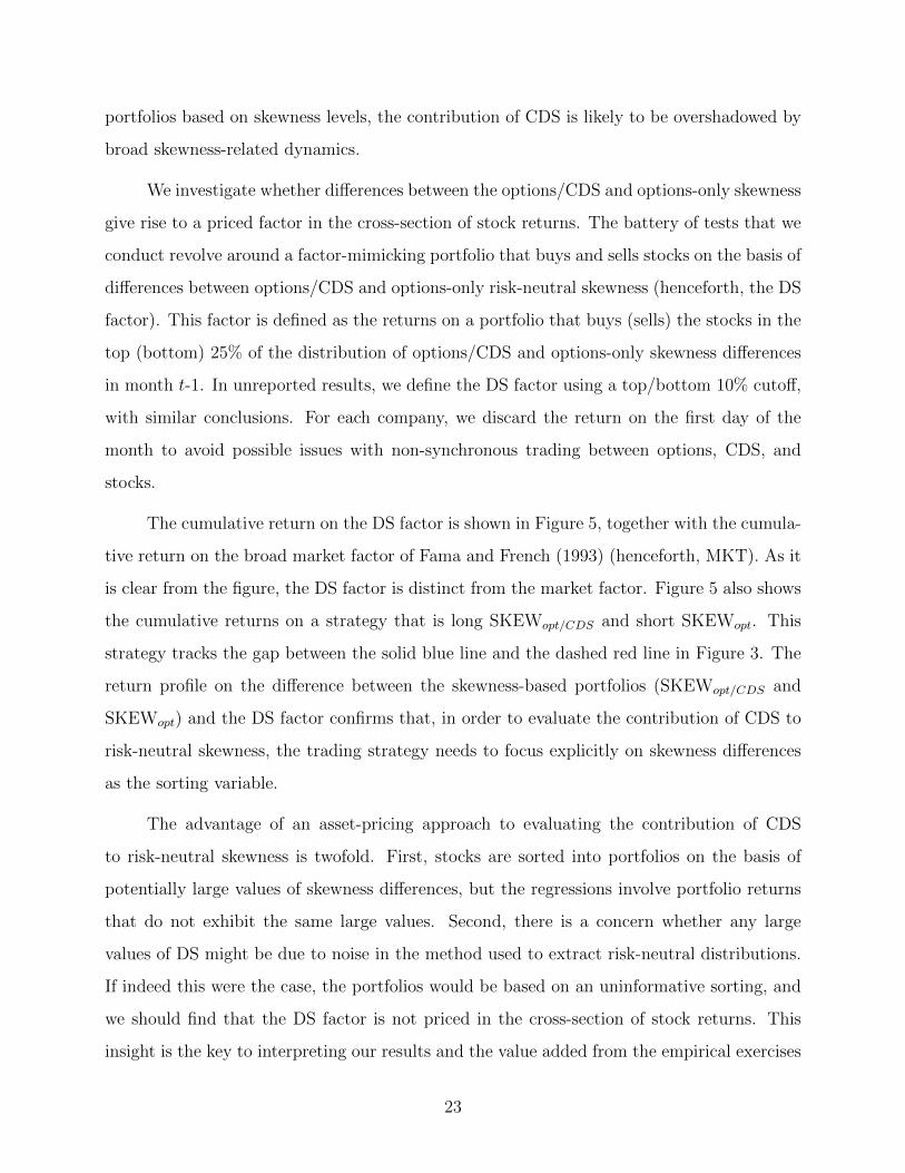
The cumulative return on the DS factor is shown in Figure 5, together with the cumula-

tive return on the broad market factor of Fama and French (1993) (henceforth, MKT). As it

is clear from the figure, the DS factor is distinct from the market factor. Figure 5 also shows

the cumulative returns on a strategy that is long SKEWopt/CDS and short SKEWopt. This

strategy tracks the gap between the solid blue line and the dashed red line in Figure 3. The

return profile on the difference between the skewness-based portfolios (SKEWopt/CDS and

SKEWopt) and the DS factor confirms that, in order to evaluate the contribution of CDS to

risk-neutral skewness, the trading strategy needs to focus explicitly on skewness differences

as the sorting variable.

The advantage of an asset-pricing approach to evaluating the contribution of CDS

to risk-neutral skewness is twofold. First, stocks are sorted into portfolios on the basis of

potentially large values of skewness differences, but the regressions involve portfolio returns

that do not exhibit the same large values. Second, there is a concern whether any large

values of DS might be due to noise in the method used to extract risk-neutral distributions.

If indeed this were the case, the portfolios would be based on an uninformative sorting, and

we should find that the DS factor is not priced in the cross-section of stock returns. This

insight is the key to interpreting our results and the value added from the empirical exercises

23

that follow.

As mentioned in Section 4.1, we interpret our results in terms of moderate-jump risk.

If DS were expressing the risk of jumps for the intermediate part of the distribution, a

high (in absolute value) difference between options/CDS and options-only skewness should

foreshadow a higher incidence of moderate-jump risk in the near future.

In the top charts of Figure 6, we show the fraction of intermediate-return variance that

is explained by jumps across deciles of differences between options/CDS and options-only

skewness. Variance (σ2) is the rolling sum of squared 15-minute returns between 9:30-16:00

daily in months t+1 to t+3. The non-jump component of variance (σ2nj) is given by the

MedRV estimator of Andersen, Dobrev, and Schaumburg (2012), and the fraction of variance

due to jumps is φ =σ2−σ2

nj

σ2 . The variance measures are computed using intermediate returns,

that is returns between the 10th–40th and 60th–90th percentiles of the daily distribution of

returns. We expect the fraction of intermediate-return variance explained by jumps to be

higher when the absolute value of DS is larger. As a result, the fraction of variance explained

by jumps should have a U-shaped pattern across DS deciles, which is what Figure 6 shows.10

We provide additional evidence that the DS factor is related to moderate-jump risk

in Figure 7. We compute the change in the probability of intermediate returns under the

options/CDS distribution relative to the options-only distribution, and we present the average

(top chart) and the 90th percentile (bottom chart) of this change in probabilities across DS

deciles.11 If the DS factor expressed moderate-jump risk, the increase in intermediate-returns

probabilities should be larger in the top and bottom DS deciles. As shown in Figure 7, this is

the case. The probability of intermediate returns is, on average, slightly more than 2% higher

10 In unreported results (available upon request), we find that the U-shaped pattern is not present whenconsidering the three months up to the DS formation period.

11 Intermediate returns are defined as those in the intervals [−2σ,−0.5σ] and [0.5σ, 2σ], where σ is thevolatility of the distribution. The probability of intermediate returns under the options/CDS distribu-tion is P intopt/CDS = P [r < 2σopt/CDS ]−P [r < 0.5σopt/CDS ]+P [r < −0.5σopt/CDS ]−P [r < −2σopt/CDS ],where r indicates returns. The probability of intermediate returns under the options-only distribution(P intopt ) is defined in a similar way, with σopt replacing σopt/CDS . The increase in the probability of inter-

mediate returns under the options/CDS distribution is defined as ∆P = lnP int

opt/CDS

P intopt

. When computing

the increase in the probability of intermediate positive returns, the interval we consider is [0.5σ, 2σ]. Forthe increase in the probability of intermediate negative returns, the interval is [−2σ,−0.5σ]. The DSdeciles and the probability increases are as of month t.

24

in the bottom DS decile, and about 1% higher in the top DS decile. At the 90th percentile,

the increase is more than 5% and about 3% in the bottom and top deciles, respectively.

The sign of the difference between options/CDS and options-only skewness indicates

whether moderate jumps are likely to be positive or negative. As illustrated in Figure 8, a

lower skewness translates into a shift of the probability mass to the right. This shift is also

evident in Figure 2, which corresponds to a day when the options/CDS skewness is much

more negative than the options-only skewness, hence the DS measure is large and negative.

The options/CDS distribution indicates a higher likelihood of intermediate positive returns.

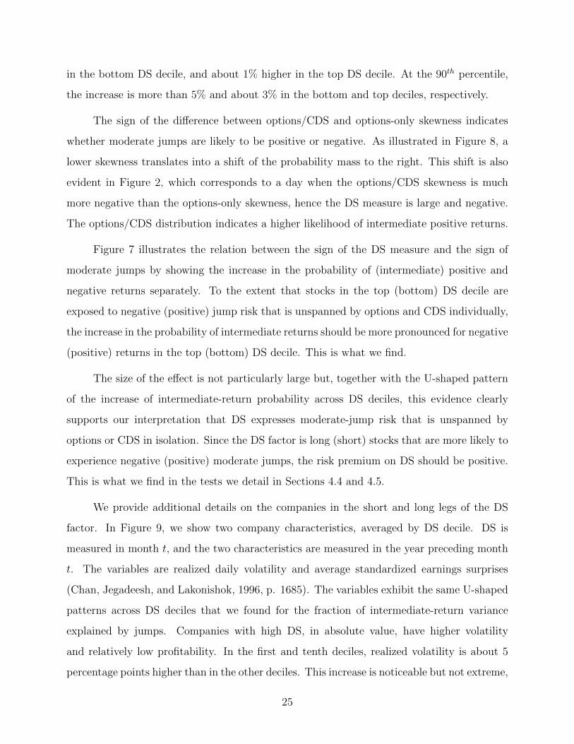
Figure 7 illustrates the relation between the sign of the DS measure and the sign of

moderate jumps by showing the increase in the probability of (intermediate) positive and

negative returns separately. To the extent that stocks in the top (bottom) DS decile are

exposed to negative (positive) jump risk that is unspanned by options and CDS individually,

the increase in the probability of intermediate returns should be more pronounced for negative

(positive) returns in the top (bottom) DS decile. This is what we find.

The size of the effect is not particularly large but, together with the U-shaped pattern

of the increase of intermediate-return probability across DS deciles, this evidence clearly

supports our interpretation that DS expresses moderate-jump risk that is unspanned by

options or CDS in isolation. Since the DS factor is long (short) stocks that are more likely to

experience negative (positive) moderate jumps, the risk premium on DS should be positive.

This is what we find in the tests we detail in Sections 4.4 and 4.5.

We provide additional details on the companies in the short and long legs of the DS

factor. In Figure 9, we show two company characteristics, averaged by DS decile. DS is

measured in month t, and the two characteristics are measured in the year preceding month

t. The variables are realized daily volatility and average standardized earnings surprises

(Chan, Jegadeesh, and Lakonishok, 1996, p. 1685). The variables exhibit the same U-shaped

patterns across DS deciles that we found for the fraction of intermediate-return variance

explained by jumps. Companies with high DS, in absolute value, have higher volatility

and relatively low profitability. In the first and tenth deciles, realized volatility is about 5

percentage points higher than in the other deciles. This increase is noticeable but not extreme,

25

consistent with the hypothesis that DS relates to moderate rather than large jumps. In line

with the higher volatility, the profitability also indicates that these companies tend to grow

less than the other firms in our sample.

Note that, while the companies in the top and bottom DS deciles have noticeably higher

volatility and lower SUE than other companies in the sample, the variation across DS deciles

is relatively small relative to sample variation. Specifically, realized volatility for high-DS

companies is about 5 percentage points higher than for the other deciles and equal to about

37%. Before averaging by DS decile, the sample median and 75% percentile volatilities are

about 28% and 40%, respectively. As for SUE, the averages in the first and tenth DS deciles

are about 0 and -0.07. Before averaging by DS decile, the sample median and the 25%

percentile are about 0.25 and -0.29. These figures confirm that the companies in the top and

bottom DS deciles are only moderately riskier than those in the remainder of the sample,

consistent with out interpretation that DS expresses the risk of moderate jumps.

Having established that the DS factor is related to moderate-jump risk, we now im-

plement a series of time-series and cross-sectional tests to evaluate whether the DS factor

commands a risk premium in the cross-section of stock returns.

4.4 Benefits of including CDS: Time-series evidence

The tests we conduct in this section focus on whether existing asset-pricing factors can explain

the returns of the DS factor. In the context of asset pricing tests, the intercept of a time

series regression represents a risk-adjusted average return, which can be interpreted as a risk

premium. If the estimated intercept is statistically different from zero, then we conclude that

the factors included in the time-series regression cannot fully account for the returns of the

DS factor.

We fit the following regression model to the data:

DSt = α +N∑i=1

βifit + εt, (10)

where α is the intercept (our parameter of interest), f it are the factors discussed below, and

26

εt is the error term. We report heteroscedasticity-consistent standard errors for all estimated

parameters, following White (1980).

We use a large number of relevant asset-pricing factors, including the five Fama and

French (2015) factors (the market, MKT, size, SMB, book-to-market, HML, profitability,

RMW, and investment, CMA), the Carhart (1997) momentum factor (UMD) and Pastor

and Stambaugh (2003) liquidity factor (LIQ). The long run and short run reversals factors,

LT REV and ST REV respectively, capture the effect of past and recent stock performance

on current stock returns (see, among others, Fama and French, 1996 and Novy-Marx, 2012,

and references therein). ∆VIX and ∆VIX2 are replicating portfolios for changes and squared

changes in the implied volatility index VIX, VRP is the replicating portfolio for Bollerslev,

Tauchen, and Zhou (2009)’s variance risk premium, and ∆CDXHY is the changes in the

spread of the CDX high-yield CDS index to control for aggregate default risk.12 We also

include the SKEWopt/CDS factor to ensure that the results are not driven by skewness.

The DS factor has a moderate positive correlation (0.27) with the market factor (MKT)

and a negative correlation with ∆VIX (-0.33), UMD (-0.38), and ∆CDXHY (-0.38). The skew-

ness factors SKEWopt/CDS and SKEWopt are highly correlated (0.99), though the correlation

of DS with both SKEWopt/CDS (0.52) and SKEWopt (0.53) is only moderate. The BKM-

skewness factor SKEWBKM is weakly correlated with DS (0.28) and moderately correlated

with SKEWopt/CDS (0.52) and SKEWopt (0.53).

We report the time series test results in Tables 8 (for the full sample) and 9 (for 2008

to 2011). The first column of Table 8 shows that, when using a small set of factors that

includes MKT, SMB, HML, UMD, LIQ, and ∆VIXrepl, the intercept – the risk adjusted

average return – is about 0.3% per month and is statistically significant at the 10% level.

The intercept remains about the same as we include progressively more factors, and the

statistical significance improves to the 5% level. The inclusion of the SKEWopt/CDS factor

improves the adjusted R2 from 39% to 44%. When we substitute the factor with SKEWBKM ,

12 The replicating portfolio for VIX changes is described in footnote 9. The replicating portfolios forsquared VIX changes and for the variance risk premium are built in exactly the same manner. The onlydifference is that stocks are sorted into portfolios using the coefficients on squared VIX changes and onthe variance risk premium, respectively, rather than on VIX changes.

27

the R2 declines back to 39%. A pertinent question is which leg of the DS portfolio is delivering

the results. In columns (6) and (7) of Table 8, we regress the returns of the long leg and

of the short leg, respectively, on the full set of factors. We observe the following. First, the

risk-adjusted average return of the DS portfolio is driven by the long leg. Second, both legs

load heavily on the MKT factor, which results in high adjusted R2s. Finally, both legs are

highly correlated with ∆VIX2repl and the SKEWopt/CDS factor.

In Table 9, we restrict our sample to the 2008-2011 period. Focusing on this period of

heightened financial uncertainty, we find that the risk-adjusted average return is noticeably

higher, ranging between 0.8% to 1.1% per month. The statistical significance is about the

same or stronger, with the exception of the specification with the smallest set of risk factors.

While larger, the adjusted R2 pattern is similar to what we observed in Table 8. In contrast

to what we observe in the previous table, columns (6) and (7) imply that the short leg is

driving the results. CDS spreads are informative about default risk during times of financial

stress.

Our estimates of the risk-adjusted average returns for the DS factor are comparable

with the expected skewness premium estimates of Rehman and Vilkov (2012) and Stilger,

Kostakis, and Poon (2017) . Both studies find positive skewness premia in the neighborhood

of 0.5% per month.

Finally, we would like to emphasize that the returns on the DS portfolio are gross of

transaction costs, and shorting fees might be elevated for risky stocks, especially at times

of market stress. As such, the estimated risk premia should be considered an upper bound

to the actual risk premium. However, we should also emphasize that our asset pricing tests

are meant to evaluate whether combining option prices and CDS spreads provides additional

information relative to the standard methods for extracting risk-neutral distributions for

individual stocks. The presence of transaction costs does not detract from our finding that

combining options and CDS spreads does provide information about the cross-section of

stocks. Transaction costs affect whether one can profitably trade on the information.

In this section, we examined the economic significance of the DS factor through the lens

of time-series asset pricing tests. Our findings show that the standard factors do not fully

28

account for the DS factor, since the estimates for the intercept are statistically significant.

4.5 Benefits of including CDS: Cross-sectional evidence

In this section, we carry out a second set of tests where we use the two-stage method of

Fama and MacBeth (1973). This method allows us to introduce stock-level characteristics.

Including characteristics in asset-pricing tests is crucial, since they can proxy for risk exposure

(see, for instance, Daniel and Titman, 1997 and Daniel, Titman, and Wei, 2001).

The first stage of the Fama and MacBeth (1973) procedure estimates the sensitivity of

the portfolio returns to the factors with a series of portfolio-specific time-series regressions:

rjt − rft = αj +

N∑i=1

βji fit + εjt , ∀j (11)

where rjt is the return on portfolio j, rft is the risk-free rate, and f it is one of the N factors

included. We consider 35 portfolios: 10 decile portfolios based on the distributions of DS in

month t-1, and the replication of the 25 size/book-to-market portfolios of Fama and French

(1993) using stocks for which we can calculate the volatility spreads of Bali and Hovakimian

(2009) and the implied-volatility smirk of Xing, Zhang, and Zhao (2010).

The second step of the Fama and MacBeth (1973) methodology uses cross-sectional

regressions to evaluate how differences in the estimated factor loadings explain excess returns:

rjt − rft = λ0

t +N∑i=1

λitβji +

K∑k=1

φkγjt−1,k + εj,∀t, (12)

where λ0t is the pricing error at time t, λit is the risk premium on factor i at time t, βjt

are the estimates from the first step, γjt−1,k is characteristic k for portfolio j as of time t-1

(calculated as the average of stock-level characteristics), and φk is the regression coefficient

for characteristic γjt−1,k. The risk premium on factor f it is computed as the average of the

coefficients from the T cross-sectional regressions, and its statistical significance is assessed

29

with Shanken (1992)-adjusted standard errors:

λi =1

T

T∑t=1

λit. (13)

The characteristics we consider are related to higher-moment risks in stock and option

returns, and have been shown to explain the cross sections of equity and option returns:

idiosyncratic volatility (Ang, Hodrick, Xing, and Zhang, 2006), volatility spreads (Bali and

Hovakimian, 2009), the implied-volatility smirk of Xing, Zhang, and Zhao (2010), the changes

in call and put implied volatility of An, Ang, Bali, and Cakici (2014), and the tail covariance

between stock market returns and company-specific returns introduced by Bali, Cakici, and

Whitelaw (2014). In addition, we include the 5-year CDS spread to evaluate whether the

contribution of the DS factor to the cross-section of returns is explained by default risk.

In the Fama-MacBeth procedure, the risk premia are identified from cross-sectional

variations in factor sensitivities, and our cross section includes 35 portfolios. As such, each

specification we discuss includes only a subset of the factors we use in the time series tests,

and we study various combinations of factors and characteristics to ensure that our findings

are robust. We present the first set of results in Table 10, where we keep the factors constant,

but change the set of characteristics included in the regression. In the full sample, the risk

premium on DS is statistically significant at the 5% level and equal to 0.5% per month. It

is comparable to the intercept in the time-series regressions of DS on other factors.13 In

line with Ang, Hodrick, Xing, and Zhang (2006), we find that stocks with high idiosyncratic

volatility have lower returns. In addition, controlling for skewness using either SKEWopt/cds

or SKEWBKM factors does not affect our findings. In the 2008-2011 sub-sample, DS factor

commands a higher premium, around 1% per month, which is in line with our time-series

findings. We find that the estimated coefficients for ∆cvol and ∆pvol (changes in call or

put implied volatilities) have the same signs as in An, Ang, Bali, and Cakici (2014) and are

13 The risk premia on most factors are statistically not different from zero. This is not surprising, sincethe test portfolios we use are designed to generate cross-sectional dispersion in risk sensitivity to the DSfactor. Hence the test is designed to capture whether the risk premium on the DS factor is absorbed byother factors. The 25 Fama-French portfolios are meant to generate cross-sectional sensitivity to SMBand HML factors. However, since the mean returns to these two factors are statistically not differentfrom zero over the sample period, we do not expect to observe a risk premium for either factor.

30

statistically significant in several instances during this period.

Studies such as Acharya and Johnson (2007), Ni and Pan (2011), and Han and Zhou

(2011) indicate the presence of information flows from the CDS market to the equity market.

Our results about the DS factor are unlikely to be driven by such flows. We include CDS

spreads in our cross-sectional regression and do not observe a statistically significant coeffi-

cient for the spreads. Moreover, we skip the first return of the month in building the test

portfolios, which eliminates the observation most likely affected by the delayed information

flow.

In Table 11 we keep the set of characteristics constant and change the factors. We use

either the three or the five Fama-French factors; see Fama and French (1993, 2015). In both

the full sample and in the 2008-2011 sub-sample, the estimated DS risk premium remains

comparable to the values reported in Table 10. In model (3), the estimated DS premium is

statistically zero. However, the asset pricing test is rejected for model (3), since the estimated

pricing error is significantly different from zero.

The cross-sectional evidence presented in this section corroborate the time-series evi-

dence reported in Section 4.4. In addition, our cross-sectional results demonstrate robustness

of DS premia to the inclusion of stock characteristics in asset pricing tests.

4.6 Robustness

We evaluate the sensitivity of our findings to changes in default thresholds and to two addi-

tional CDS tenors. We report these results in Table 12. So far, we have presented empirical

evidence based on the thresholds shown in Panel A, Table 4. In columns 1 to 6 of Table

12, we report results based on the default thresholds shown in Panel B, Table 4. The es-

timated time-series intercepts are slightly smaller than those reported in Tables 8 and 9.

When compared with the findings presented in Sections 4.4 and 4.5, these results highlight

the importance of choosing default thresholds based on company characteristics, such as size

and leverage. The intercepts for 120% of the mean for 2008-2011 sub-sample and 80% of the

mean in the full sample are statistically significant, and most of the remaining marginally fail

31

the statistical significance test. The adjusted R2s are comparable to our previously reported

values. The size of the DS risk premium is similar to those shown in Tables 10 and 11 in

both full sample and in the 2008-2011 sub-sample.

As noted by Chen, Fleming, Jackson, Li, and Sarkar (2011), trading liquidity in the CDS

market is concentrated in the five-year tenor. Therefore, we focus on risk-neutral distribu-

tions extracted using options and the appropriately compounded five-year CDS spread, even

though the horizon to which the distribution refers is three months. Even if five-year spreads

are the most liquid and thus more likely to have a higher signal-to-noise ratio, Friewald, Wag-

ner, and Zechner (2014) find that the term-structure of CDS spreads is informative about

the equity risk premium. We repeat our analysis using either one-year CDS spreads from

Markit or three-month CDS spreads, obtained by linearly extrapolating log-CDS spreads

with maturities between six months and 10 years. The last four columns of Table 12 show

that the results are robust to using alternative CDS tenors. In both time-series and cross-

sectional regressions, the size of the estimated intercepts and DS premia are comparable to

our reported results. The estimated intercepts have larger t statistics compared with those

reported in Tables 8 and 9. In Fama-MacBeth regressions, we slightly lower t statistics for

the DS premia.

Harvey, Liu, and Zhu (2016) document the pervasive presence of data mining in many

cross-sectional results in the asset pricing literature. They recommend setting a higher bar for

asset-pricing tests evaluating cross-sectional factors, a t statistics in excess of 3, translating

into statistical significance between 97.5% and 99% for cross-sectional tests with four factors.

Increasing the number of factors implies far more stringent significance criteria. However,

they limit their recommendation to new and purely empirical results. They explicitly state

that micro-founded, theoretically-motivated results need not pass their proposed bar.

In this study, we contribute to a mature literature. The link between skewness and

equity returns is empirically and theoretically well established. There are a number of papers

– we have cited Rehman and Vilkov (2012), Conrad, Dittmar, and Ghysels (2013), and Stilger,

Kostakis, and Poon (2017), among others – that specifically investigate the link between risk-

neutral, firm-specific skewness and the cross-section of returns. In addition, studies such as

32

Chabi-Yo, Leisen, and Renault (2014), Feunou, Jahan-Parvar, and Tedongap (2013), and

Feunou, Jahan-Parvar, and Okou (Forthcoming) explicitly derive equilibrium asset pricing

models for skewness preferences.14 As such, we contribute to a clearly theoretically-founded

line of research.

In addition, the relation between the momentum strategy returns and the options/CDS

portfolio returns discussed in Section 4.2 is relevant to address Harvey, Liu, and Zhu (2016)

concerns. The evidence we find on the relation between momentum and skewness returns is

incidental to the central topic of our work, yet it fits naturally in the overall discussion. It is

unlikely that both our main difference-in-skewness results and the link between momentum

and skewness returns are the outcome of data mining.

5 Conclusions

We develop a new method to extract the risk-neutral distribution of firm-specific expected

stock returns. Traditionally, risk neutral distributions are based on option prices. In the

case of stock indexes, like the S&P 500, the number of actively traded options with out-of-

the-money strikes is large enough that risk-neutral distributions are informative about tail

risk. For individual companies, however, only options with strike price close to the current

stock price are actively traded. Our method combines options and credit default swaps

(CDS) to extract risk-neutral distributions. By construction, the options/CDS-implied risk-

neutral distributions reflect the default risk embedded in CDS spreads. In addition, the

combination of options and CDS is also informative about the intermediate part of the risk-

neutral distribution. This part of the distribution is influenced by moderate-sized, signed

jumps. Options and CDS individually offer limited information about expected moderate-

sized jumps. Jointly, however, options and CDS help us span this part of a risk-neutral

distribution by providing a more informative skewness measure.

We evaluate our method with a series of asset pricing tests that revolve around a

factor that buys (sells) stocks with large differences between options/CDS and options-only

14 Guidolin and Timmermann (2008) contribute to this literature in an international, multi-country context.

33

skewness. This factor is long (short) in stocks exposed to negative (positive) moderate-sized

jump risk that is unspanned by options and CDS individually. After controlling for a large

set of asset pricing factors and stock characteristics, we find that the factor commands a risk

premium of 0.5% per month. While the results are robust to different assumptions about key

inputs of the method, we find that it is important to choose default thresholds that reflect

the size and leverage of a company.

34

References

Acharya, V., and T. Johnson, 2007, “Insider trading in credit derivatives,” Journal of Fi-nancial Economics, 84(1), 110–141.

Aıt-Sahalia, Y., and A. Lo, 1998, “Nonparametric estimation of state-price densities implicitin financial asset prices,” Journal of Finance, 53(2), 499–547.

Amaya, D., P. Christoffersen, K. Jacobs, and A. Vasquez, 2015, “Does realized skewnesspredict the cross-section of equity returns?,” Journal of Financial Economics, 118(1), 135–167.

An, B.-J., A. Ang, T. Bali, and N. Cakici, 2014, “The joint cross section of stocks andoptions,” Journal of Finance, 69(5), 2279–2337.

Andersen, T., D. Dobrev, and E. Schaumburg, 2012, “Jump-robust volatility estimation usingnearest neighbor truncation,” Journal of Econometrics, 169(1), 75–93.

Andersen, T., N. Fusari, and V. Todorov, 2015, “Parametric inference and dynamic staterecovery from option panels,” Econometrica, 83(3), 1081–1145.

Ang, A., R. Hodrick, Y. Xing, and X. Zhang, 2006, “The cross-section of volatility andexpected returns,” Journal of Finance, 61(1), 259–299.

Arora, N., P. Ghandi, and F. Longstaff, 2012, “Counterparty credit risk and the credit defaultswap market,” Journal of Financial Economics, 103(2), 280–293.

Bakshi, G., N. Kapadia, and D. Madan, 2003, “Stock return characteristics, skew laws, andthe differential pricing of individual equity options,” Review of Financial Studies, 16(1),101–143.

Bakshi, G., and D. Madan, 2000, “Spanning and derivative-security valuation,” Journal ofFinancial Economics, 55(2), 205–238.

Bali, T., N. Cakici, and R. Whitelaw, 2014, “Hybrid tail risk and expected stock returns:When does the tail wag the dog?,” Review of Asset Pricing Studies, 4(2), 206–246.

Bali, T., and A. Hovakimian, 2009, “Volatility spreads and expected stock returns,” Man-agement Science, 55(11), 1797–1812.

Bali, T., and S. Murray, 2013, “Does risk-neutral skewness predict the cross-section of equityoption portfolio returns?,” Journal of Financial and Quantitative Analysis, 48(4), 1145–1171.

Bandi, F., and R. Reno, 2016, “Price and volatility co-jumps,” Journal of Financial Eco-nomics, 119(1), 107–146.

Barroso, P., and P. Santa-Clara, 2015, “Momentum has its moments,” Journal of FinancialEconomics, 116(1), 111–120.

35

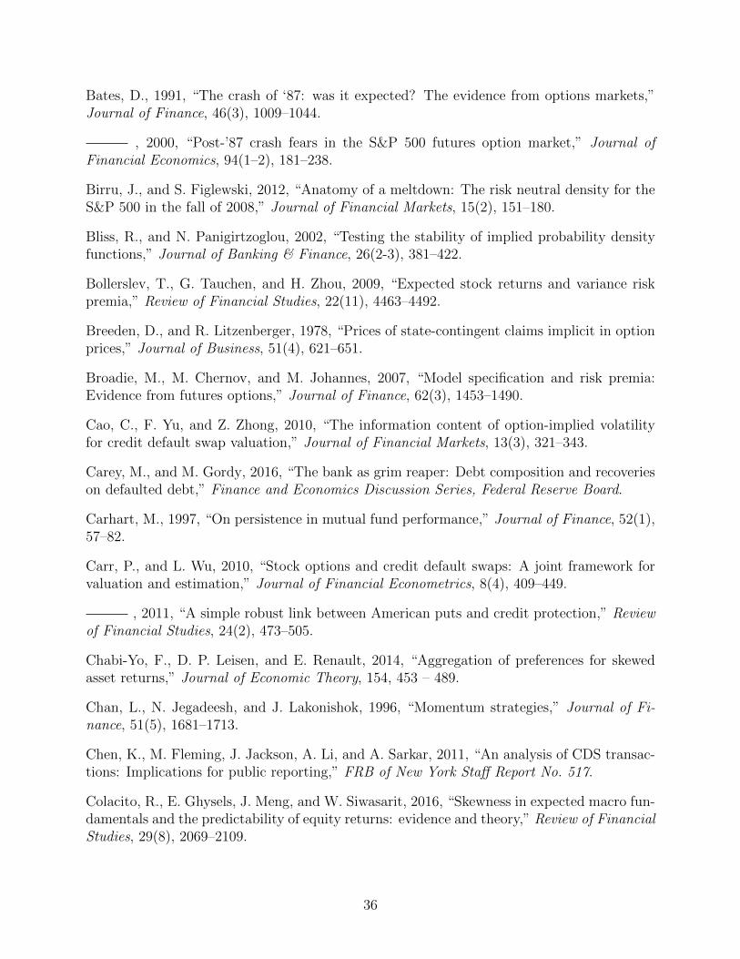
Bates, D., 1991, “The crash of ‘87: was it expected? The evidence from options markets,”Journal of Finance, 46(3), 1009–1044.

, 2000, “Post-’87 crash fears in the S&P 500 futures option market,” Journal ofFinancial Economics, 94(1–2), 181–238.

Birru, J., and S. Figlewski, 2012, “Anatomy of a meltdown: The risk neutral density for theS&P 500 in the fall of 2008,” Journal of Financial Markets, 15(2), 151–180.

Bliss, R., and N. Panigirtzoglou, 2002, “Testing the stability of implied probability densityfunctions,” Journal of Banking & Finance, 26(2-3), 381–422.

Bollerslev, T., G. Tauchen, and H. Zhou, 2009, “Expected stock returns and variance riskpremia,” Review of Financial Studies, 22(11), 4463–4492.

Breeden, D., and R. Litzenberger, 1978, “Prices of state-contingent claims implicit in optionprices,” Journal of Business, 51(4), 621–651.

Broadie, M., M. Chernov, and M. Johannes, 2007, “Model specification and risk premia:Evidence from futures options,” Journal of Finance, 62(3), 1453–1490.

Cao, C., F. Yu, and Z. Zhong, 2010, “The information content of option-implied volatilityfor credit default swap valuation,” Journal of Financial Markets, 13(3), 321–343.

Carey, M., and M. Gordy, 2016, “The bank as grim reaper: Debt composition and recoverieson defaulted debt,” Finance and Economics Discussion Series, Federal Reserve Board.

Carhart, M., 1997, “On persistence in mutual fund performance,” Journal of Finance, 52(1),57–82.

Carr, P., and L. Wu, 2010, “Stock options and credit default swaps: A joint framework forvaluation and estimation,” Journal of Financial Econometrics, 8(4), 409–449.

, 2011, “A simple robust link between American puts and credit protection,” Reviewof Financial Studies, 24(2), 473–505.

Chabi-Yo, F., D. P. Leisen, and E. Renault, 2014, “Aggregation of preferences for skewedasset returns,” Journal of Economic Theory, 154, 453 – 489.

Chan, L., N. Jegadeesh, and J. Lakonishok, 1996, “Momentum strategies,” Journal of Fi-nance, 51(5), 1681–1713.

Chen, K., M. Fleming, J. Jackson, A. Li, and A. Sarkar, 2011, “An analysis of CDS transac-tions: Implications for public reporting,” FRB of New York Staff Report No. 517.

Colacito, R., E. Ghysels, J. Meng, and W. Siwasarit, 2016, “Skewness in expected macro fun-damentals and the predictability of equity returns: evidence and theory,” Review of FinancialStudies, 29(8), 2069–2109.

36

Conrad, J., R. Dittmar, and E. Ghysels, 2013, “Ex ante skewness and expected stock returns,”Journal of Finance, 68(1), 85–124.

Cox, J., S. Ross, and M. Rubinstein, 1979, “Option pricing: A simplified approach,” Journalof Financial Economics, 7(3), 229–263.

Cremers, M., J. Driessen, and P. Maenhout, 2008, “Explaining the level of credit spreads:Option-implied jump risk premia in a firm value model,” Review of Financial Studies, 21(5),2209–2242.

Cremers, M., J. Driessen, P. Maenhout, and D. Weinbaum, 2008, “Individual stock-optionprices and credit spreads,” Journal of Banking & Finance, 32(12), 2706–2715.

Daniel, K., and T. Moskowitz, 2016, “Momentum crashes,” Journal of Financial Economics,122(2), 221–247.

Daniel, K., and S. Titman, 1997, “Evidence on the characteristics of cross sectional variationin stock returns,” Journal of Finance, 52(1), 1–33.

Daniel, K., S. Titman, and K. Wei, 2001, “Explaining the cross-section of stock returns inJapan: Factors or characteristics,” Journal of Finance, 56(2), 743–766.

DeMiguel, V., Y. Plyakha, R. Uppal, and G. Vilkov, 2013, “Improving portfolio selection us-ing option-implied volatility and skewness,” Journal of Financial and Quantitative Analysis,48(6), 1813–1845.

Dennis, P., and S. Mayhew, 2002, “Risk-neutral skewness: Evidence from stock options,”Journal of Financial and Quantitative Analysis, 37(3), 471–493.

Driessen, J., P. Maenhout, and G. Vilkov, 2009, “The price of correlation risk: Evidencefrom equity options,” Journal of Finance, 64(3), 1377–1406.

Duffie, D. Singleton, K., 2003, Credit risk: Pricing, measurement, and management. Prince-ton University Press, Princeton, N.J., 1 edn.

Fama, E., and K. French, 1993, “Common risk factors in the returns on stocks and bonds,”Journal of Financial Economics, 33(1), 3–56.

, 1996, “Multifactor explanations of asset pricing anomalies,” Journal of Finance,51(1), 55–84.

, 2015, “A five-factor asset pricing model,” Journal of Financial Economics, 116(1),1–22.

Fama, E., and J. MacBeth, 1973, “Risk, return, and equilibrium: Empirical tests,” Journalof Political Economy, 81(3), 607–636.

Fan, H., and S. Sundaresan, 2000, “Debt valuation, renegotiation, and optimal dividendpolicy,” Review of Financial Studies, 13(4), 1057–1099.

37

Feunou, B., M. Jahan-Parvar, and C. Okou, Forthcoming, “Downside variance risk premium,”Journal of Financial Econometrics.

Feunou, B., M. Jahan-Parvar, and R. Tedongap, 2013, “Modeling market downside volatil-ity,” Review of Finance, 17(1), 443–481.

, 2016, “Which parametric model for conditional skewness?,” European Journal ofFinance, 22(13), 1237–1271.

Figlewski, S., 2010, “Estimating the implied risk-neutral density for the US market portfolio,”in “Volatility and time series econometrics: essays in honor of Robert Engle”, edited by T.Bollerslev, J. Russell, and M.Watson. Oxford University Press.

Friewald, N., C. Wagner, and J. Zechner, 2014, “The cross-section of credit risk premia andequity returns,” Journal of Finance, 69(6), 2419–2469.

Garleanu, N., L. Pedersen, and A. Poteshman, 2009, “Demand-based option pricing,” Reviewof Financial Studies, 22(10), 4259–4299.

Ghysels, E., A. Plazzi, and R. Valkanov, 2016, “Why invest in emerging markets? The roleof conditional return asymmetry,” Journal of Finance, 71(5), 2145–2192.

Guidolin, M., and A. Timmermann, 2008, “International asset allocation under regimeswitching, skew, and kurtosis preferences,” Review of Financial Studies, 21(2), 889–935.

Han, B., and Y. Zhou, 2011, “Term structure of credit default spreads and cross-section ofstock returns,” Working paper.

Hansen, B., 1994, “Autoregressive conditional density estimation,” International EconomicReview, 35(3), 705–730.

Harvey, C., Y. Liu, and H. Zhu, 2016, “... and the cross-section of expected returns,” Reviewof Financial Studies, 29(1), 5–68.

Harvey, C., and A. Siddique, 2000, “Conditional skewness in asset pricing tests,” Journal ofFinance, 55, 1263–1295.

Jackwerth, J., and M. Rubinstein, 1996, “Recovering probability distributions from optionprices,” Journal of Finance, 51(5), 1611–1631.

JPMorgan, 2001, “Par credit default swap spread approximation from default probabilities,”JPMorgan Securities Inc. Report.

Khozan, R., A. Neuberger, and P. Schneider, 2013, “The skew risk premium in the equityindex market,” Review of Financial Studies, 26(9), 2174–2203.

Kim, T., and H. White, 2004, “On more robust estimation of skewness and kurtosis,” FinanceResearch Letters, 1(1), 56–73.

38

Longstaff, F., 1995, “Option pricing and the martingale restriction,” Review of FinancialStudies, 8(4), 1091–1124.

Madan, D., and F. Milne, 1994, “Contingent claims valued and hedged by pricing and in-vesting in a basis,” Mathematical Finance, 4(3), 223–245.

Neuberger, A., 2012, “Realized skewness,” Review of Financial Studies, 25(11), 3423–3455.

Ni, S., and J. Pan, 2011, “Trading puts and CDS on stocks with short sale ban,” Workingpaper.

Novy-Marx, R., 2012, “Is momentum really momentum?,” Journal of Financial Economics,103(3), 429–453.

Pastor, L., and R. Stambaugh, 2003, “Liquidity risk and expected stock returns,” Journal ofPolitical Economy, 111(3), 642–685.

Patton, A., 2004, “On the out-of-sample importance of skewness and asymmetric dependencefor asset allocation,” Journal of Financial Econometrics, 2(1), 130–168.

Patton, A., and K. Sheppard, 2015, “Good volatility, bad volatility: Signed jumps and thepersistence of volatility,” Review of Economics and Statistics, 97(3), 683–697.

Rehman, Z., and G. Vilkov, 2012, “Risk-neutral skewness: Return predictability and itssources,” Working paper, Frankfurt University.

Rubinstein, M., 1994, “Implied binomial trees,” Journal of Finance, 49(3), 771–818.

Santa-Clara, P., and A. Saretto, 2009, “Option strategies: Good deals and margin calls,”Journal of Financial Markets, 12(3), 391–417.

Shanken, J., 1992, “On the estimation of beta-pricing models,” Review of Financial Studies.

Shimko, D., 1993, “Bounds of probability,” Risk, 6, 33–37.

Stilger, P., A. Kostakis, and S. Poon, 2017, “What does risk-neutral skewness tell us aboutfuture stock returns?,” Management Science, 63(6), 1814–1834.

White, H., 1980, “A heteroskedasticity-consistent covariance matrix estimator and a directtest for heteroskedasticity,” Econometrica, 48(4), 817–838.

Xing, Y., X. Zhang, and R. Zhao, 2010, “What does the individual option volatility smirktell us about future equity returns?,” Journal of Financial and Quantitative Analysis, 45(3),641–662.

Zhang, B., H. Zhou, and H. Zhu, 2009, “Explaining credit default swap spreads with theequity volatility and jump risks of individual firms,” Review of Financial Studies, 22(12),5099–5131.

39

Figure 1: The contribution of options and CDS to risk-neutral return distributions

The figure provides a stylized illustration of the contribution that options and CDS give to the risk-neutral

distribution of returns. The cumulative probabilities extracted from option prices (Section 3.1) drive the

central part of the distribution. The red markers correspond to traded strikes, which are normally clustered

close to the current stock price. The location of the markers on the density function indicates which part of

the distribution each option is informative about. The CDS-implied default probability (Section 3.2) drives

the distribution up to the default threshold (Section 3.3).

Default threshold

CDS-implied probability of default0.2

5.5

.75

Pro

babi

lity

dens

ity

-2 -1 0 1 2Log returns

40

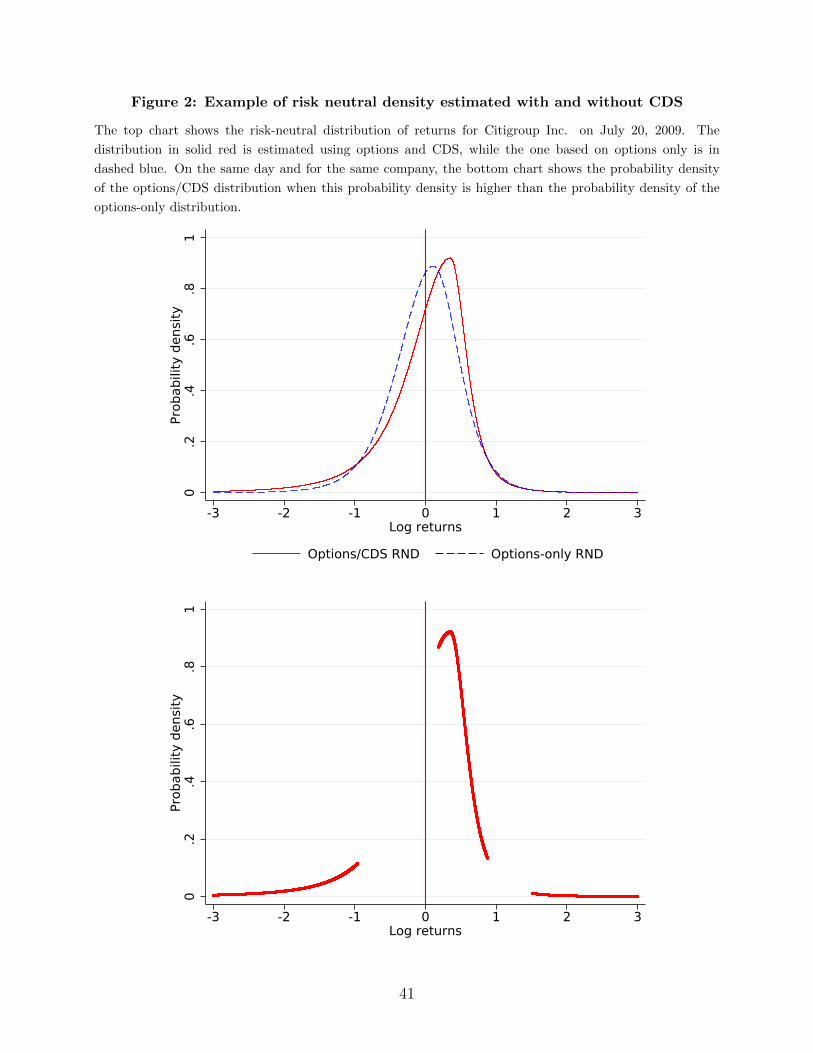
Figure 2: Example of risk neutral density estimated with and without CDS

The top chart shows the risk-neutral distribution of returns for Citigroup Inc. on July 20, 2009. The

distribution in solid red is estimated using options and CDS, while the one based on options only is in

dashed blue. On the same day and for the same company, the bottom chart shows the probability density

of the options/CDS distribution when this probability density is higher than the probability density of the

options-only distribution.

0.2

.4.6

.81

Prob

abili

ty d

ensi

ty

-3 -2 -1 0 1 2 3Log returns

Options/CDS RND Options-only RND

0.2

.4.6

.81

Prob

abili

ty d

ensi

ty

-3 -2 -1 0 1 2 3Log returns

41

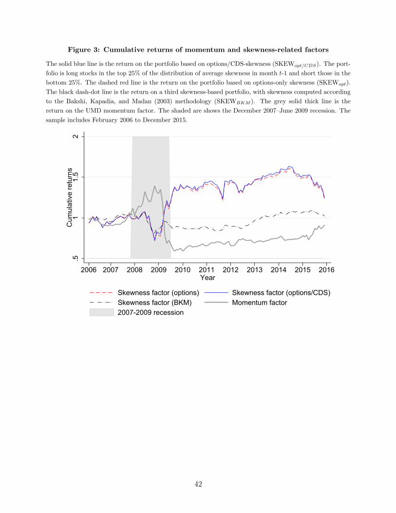
Figure 3: Cumulative returns of momentum and skewness-related factors

The solid blue line is the return on the portfolio based on options/CDS-skewness (SKEWopt/CDS). The port-

folio is long stocks in the top 25% of the distribution of average skewness in month t-1 and short those in the

bottom 25%. The dashed red line is the return on the portfolio based on options-only skewness (SKEWopt).

The black dash-dot line is the return on a third skewness-based portfolio, with skewness computed according

to the Bakshi, Kapadia, and Madan (2003) methodology (SKEWBKM ). The grey solid thick line is the

return on the UMD momentum factor. The shaded are shows the December 2007–June 2009 recession. The

sample includes February 2006 to December 2015.

.51

1.5

2C

umul

ativ

e re

turn

s

2006 2007 2008 2009 2010 2011 2012 2013 2014 2015 2016Year

Skewness factor (options) Skewness factor (options/CDS)Skewness factor (BKM) Momentum factor2007-2009 recession

42

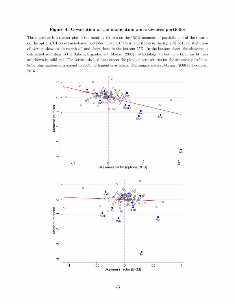
Figure 4: Covariation of the momentum and skewness portfolios

The top chart is a scatter plot of the monthly returns on the UMD momentum portfolio and of the returns

on the options/CDS skewness-based portfolio. The portfolio is long stocks in the top 25% of the distribution

of average skewness in month t-1 and short those in the bottom 25%. In the bottom chart, the skewness is

calculated according to the Bakshi, Kapadia, and Madan (2003) methodology. In both charts, linear fit lines

are shown in solid red. The vertical dashed lines center the plots on zero returns for the skewness portfolios.

Solid blue markers correspond to 2009, with months as labels. The sample covers February 2006 to December

2015.

Jan

Feb

Mar

Apr

May

Jun

Jul

Aug

Sep

OctNov

Dec

-.4-.3

-.2-.1

0.1

Mom

entu

m fa

ctor

-.1 0 .1 .2Skewness factor (options/CDS)

Jan

Feb

Mar

Apr

May

Jun

Jul

Aug

Sep

OctNov

Dec

-.4-.3

-.2-.1

0.1

Mom

entu

m fa

ctor

-.1 -.05 0 .05 .1Skewness factor (BKM)

43

Figure 5: DS factor and market factor, cumulative returns

The difference-in-skewness (DS) factor is a long/short portfolio that, in month t, buys (sells) stocks in the top

(bottom) 25% of the month t−1 distribution of skewness differences between the options/CDS- and options-

only distributions. End-of-month values for skewness are the average of the last three daily observations

within each month. The market factor is the return of the Fama-French market portfolio (Fama and French,

1993) over the risk-free rate. Cumulative returns for the DS factor are shown in solid red, and cumulative

returns for the market factor are in dashed blue. The dash-dot black line shows the cumulative returns for

a trading strategy that buys the portfolio based on options/CDS-skewness and sells the portfolio based on

options-only skewness. The sample includes February 2006 to December 2015.

.51

1.5

2C

umul

ativ

e re

turn

s

2006 2007 2008 2009 2010 2011 2012 2013 2014 2015 2016Year

DS factor Option/CDS factor minus option factorMarket factor 2007-2009 recession

44

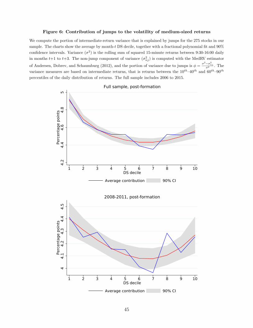
Figure 6: Contribution of jumps to the volatility of medium-sized returns

We compute the portion of intermediate-return variance that is explained by jumps for the 275 stocks in our

sample. The charts show the average by month-t DS decile, together with a fractional polynomial fit and 90%

confidence intervals. Variance (σ2) is the rolling sum of squared 15-minute returns between 9:30-16:00 daily

in months t+1 to t+3. The non-jump component of variance (σ2nj) is computed with the MedRV estimator

of Andersen, Dobrev, and Schaumburg (2012), and the portion of variance due to jumps is φ =σ2−σ2

nj

σ2 . The

variance measures are based on intermediate returns, that is returns between the 10th–40th and 60th–90th

percentiles of the daily distribution of returns. The full sample includes 2006 to 2015.

4.2

4.4

4.6

4.8

5Pe

rcen

tage

poi

nts

1 2 3 4 5 6 7 8 9 10DS decile

Average contribution 90% CI

Full sample, post-formation

44.

14.

24.

34.

44.

5Pe

rcen

tage

poi

nts

1 2 3 4 5 6 7 8 9 10DS decile

Average contribution 90% CI

2008-2011, post-formation

45

Figure 7: Increase in the probability of intermediate returns under the options/CDSdistribution, by DS decile

The figure shows the average (top chart) and 90th percentile (bottom chart) increase in the probability of

intermediate returns from the options-only distribution to the options/CDS distribution. See footnote 11 for

the definition of intermediate returns and for the calculation of the increase in probability. The DS deciles

and the probability increases are as of month t. The sample includes 2006 to 2015.

0.5

11.

52

2.5

Prob

abili

ty in

crea

se (%

)

1 2 3 4 5 6 7 8 9 10DS decile

All returns Positive returnsNegative returns

Average

02

46

Prob

abili

ty in

crea

se (%

)

1 2 3 4 5 6 7 8 9 10DS decile

All returns Positive returnsNegative returns

90th percentile

46

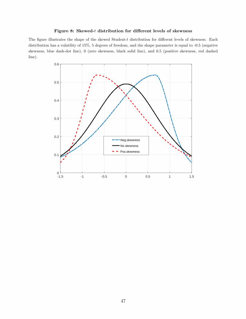
Figure 8: Skewed-t distribution for different levels of skewness

The figure illustrates the shape of the skewed Student-t distribution for different levels of skewness. Each

distribution has a volatility of 15%, 5 degrees of freedom, and the shape parameter is equal to -0.5 (negative

skewness, blue dash-dot line), 0 (zero skewness, black solid line), and 0.5 (positive skewness, red dashed

line).

-1.5 -1 -0.5 0 0.5 1 1.50

0.1

0.2

0.3

0.4

0.5

0.6

Neg.skewness

No skewness

Pos.skewness

47

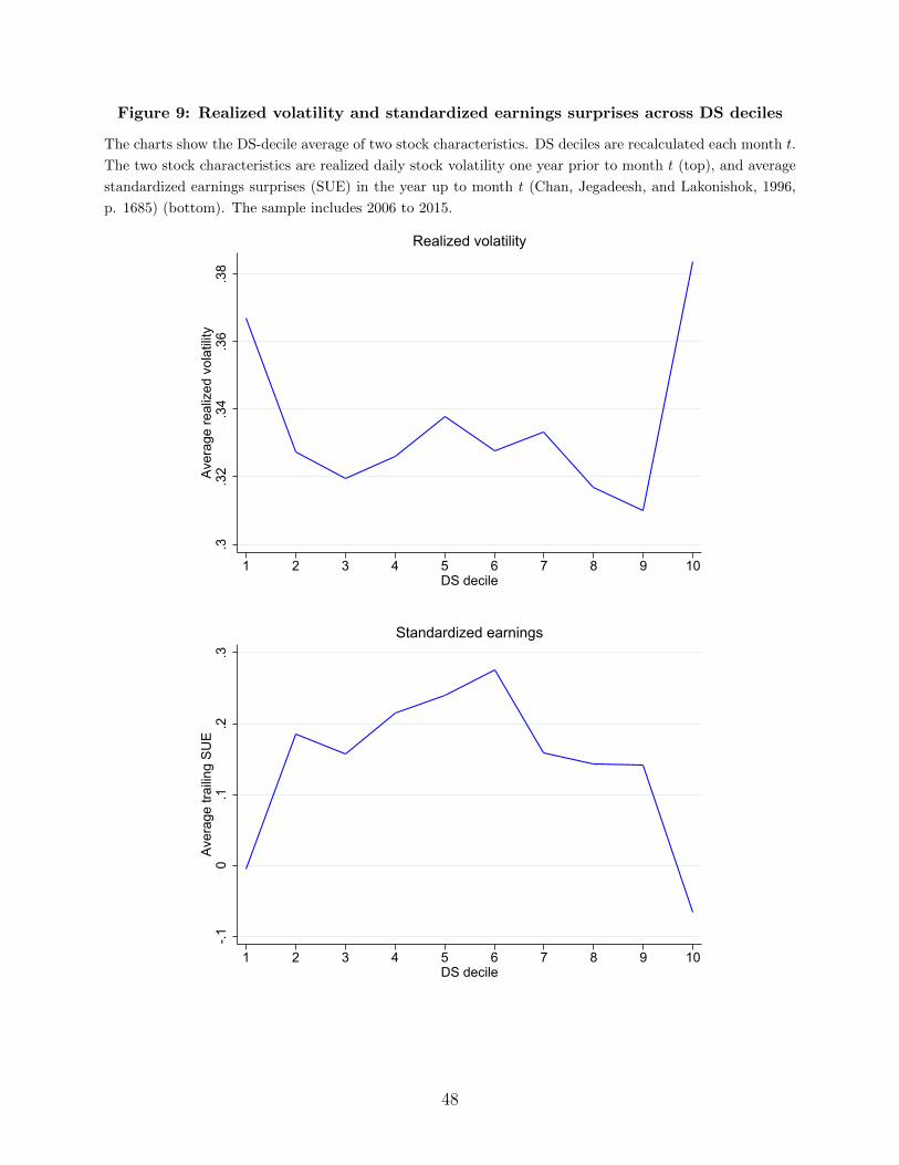
Figure 9: Realized volatility and standardized earnings surprises across DS deciles

The charts show the DS-decile average of two stock characteristics. DS deciles are recalculated each month t.

The two stock characteristics are realized daily stock volatility one year prior to month t (top), and average

standardized earnings surprises (SUE) in the year up to month t (Chan, Jegadeesh, and Lakonishok, 1996,

p. 1685) (bottom). The sample includes 2006 to 2015..3

.32

.34

.36

.38

Ave

rage

real

ized

vol

atili

ty

1 2 3 4 5 6 7 8 9 10DS decile

Realized volatility-.1

0.1

.2.3

Ave

rage

trai

ling

SU

E

1 2 3 4 5 6 7 8 9 10DS decile

Standardized earnings

48

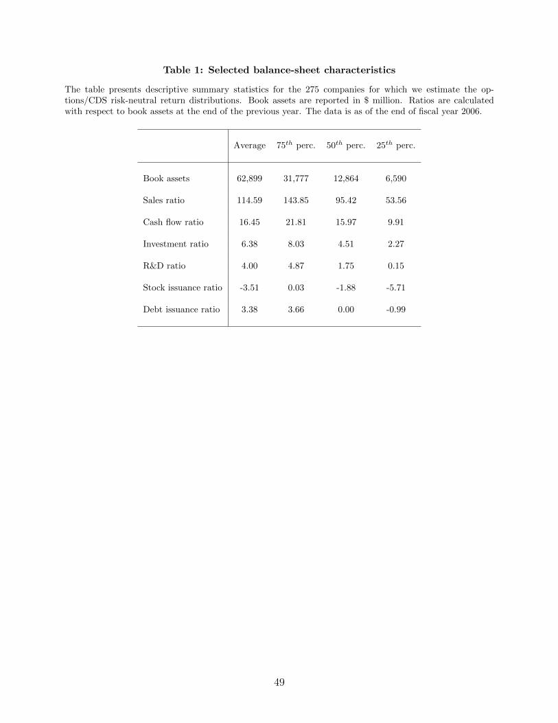
Table 1: Selected balance-sheet characteristics

The table presents descriptive summary statistics for the 275 companies for which we estimate the op-tions/CDS risk-neutral return distributions. Book assets are reported in $ million. Ratios are calculatedwith respect to book assets at the end of the previous year. The data is as of the end of fiscal year 2006.

Average 75th perc. 50th perc. 25th perc.

Book assets 62,899 31,777 12,864 6,590

Sales ratio 114.59 143.85 95.42 53.56

Cash flow ratio 16.45 21.81 15.97 9.91

Investment ratio 6.38 8.03 4.51 2.27

R&D ratio 4.00 4.87 1.75 0.15

Stock issuance ratio -3.51 0.03 -1.88 -5.71

Debt issuance ratio 3.38 3.66 0.00 -0.99

49

Table 2: Summary statistics on option-data availability

The table reports the average and median number of daily option observations, and the associated volumes,after applying the filters discussed in Section 2. The statistics are reported separately for S&P 500 indexoptions and for options on the 275 companies for which we estimate options/CDS risk-neutral distributions.The statistics are shown by call and put option types (C and P, respectively), and for different moneynesslevels. A call (put) option is out-of-the-money (OTM) if the strike price is above (below) the stock price. Aput option is deep OTM if the strike price is less than 80% of the stock price. The sample includes 2006 to2015.

Options on the S&P 500 indexCall/Put Moneyness Average obs. Median obs. Av. volume Med. volume

C ITM 5.40 4 6,541 788C OTM 12.02 11 10,772 5,825

P ITM 4.29 3 5,023 709P OTM 14.69 13 19,702 11,942P Deep OTM 8.11 6 4,074 1,312

Options on the firms we studyCall/Put Moneyness Average obs. Median obs. Av. volume Med. volume

C ITM 2.91 2 393 66C OTM 3.24 3 701 173

P ITM 2.21 2 256 48P OTM 2.51 2 427 92P Deep OTM 1.82 1 219 30

50

Tab

le3:

Illu

stra

tion

of

the

defa

ult

-ris

kin

form

ati

ven

ess

an

dtr

ad

ing

liqu

idit

yof

op

tion

san

dC

DS

Th

eta

ble

illu

stra

tes

the

info

rmat

iven

ess

abou

td

efau

ltri

skan

dth

ety

pic

al

trad

ing

liqu

idit

yof

aC

DS

an

dof

ase

tof

call

an

dp

ut

op

tion

sw

ith

diff

eren

tst

rike

pri

ces.

Th

eas

sum

pti

onis

that

the

curr

ent

stock

pri

ceis

$100,

an

dth

at

the

com

pany

def

au

lts

ifth

est

ock

pri

ced

rops

to$20.

Ase

curi

tyis

use

ful

for

char

acte

rizi

ng

the

dee

ple

ftta

ilof

ari

sk-n

eutr

al

dis

trib

uti

on

of

retu

rns

on

lyif

itis

info

rmati

veab

ou

td

efau

ltri

skan

dit

isact

ivel

ytr

ad

ed.

Sec

uri

tyO

pti

onC

DS

Opti

onty

pe

Cal

lP

ut

Opti

onst

rike

110

100

9020

110

100

9020

Typic

ally

trad

ed?

yes

yes

yes

no

yes

yes

yes

no

yes

Info

rmat

ive

abou

tth

edee

ple

ftta

il?

no

no

no

yes

no

no

no

yes

yes

51

Table 4: Default thresholds

The table shows the default thresholds we use when extracting the options/CDS risk-neutral distributions.The thresholds are estimated on a sample of 167 firms with market capitalization in excess of 100 million thatfiled for Chapter 7 or Chapter 11 between 1990 and 2015, and that delisted within 30 days of bankruptcy. Thethresholds are average cumulative returns over the three-month period leading to bankruptcy. In Panel A,they are calculated after double sorting firms based on size and leverage. Low/high leverage means leveragebelow/above the sample median. Large firms are those with market capitalization in excess of $1 billion.Panel B shows the average of the four thresholds in Panel A (the average is taken over log returns), and120% and 80% of the average. We use these thresholds in robustness tests.

Panel A – Characteristics-based thresholds

Log returnsLow leverage High leverage

Market cap < 1bn -1.68 -1.21Market cap ≥ 1bn -2.29 -2.24

Arithmetic returnsLow leverage High leverage

Market cap < 1bn -0.81 -0.70Market cap ≥ 1bn -0.90 -0.89

Panel B – Fixed thresholds

Log returns Arithmetic returnsAverage of Panel A -1.85 -0.84120% of average -2.23 -0.8980% of average -1.48 -0.77

52

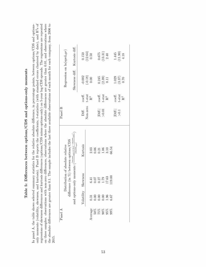
Tab

le5:

Diff

ere

nces

betw

een

op

tion

s/C

DS

an

dop

tion

s-on

lym

om

ents

Inp

anel

A,

the

tab

lesh

ows

sele

cted

sum

mar

yst

ati

stic

sfo

rth

ere

lati

veab

solu

ted

iffer

ence

,in

per

centa

ge

poin

ts,

bet

wee

nop

tion

s/C

DS

an

dop

tion

s-on

lym

omen

ts(v

olat

ilit

y,sk

ewn

ess,

and

ku

rtos

is).

Pan

elB

rep

ort

sth

eco

effici

ents

,t-

stati

stic

s(w

ith

stan

dard

erro

rscl

ust

ered

by

date

),an

dR

2s

of

regr

essi

ons

ofsk

ewn

ess

diff

eren

ces

and

ku

rtos

isd

iffer

ence

s(o

pti

on

s/C

DS

min

us

op

tion

s-on

ly)

on

5-y

ear

log-C

DS

spre

ad

s.T

he

regre

ssio

ns

are

rep

eate

don

thre

esa

mp

les:

obse

rvat

ion

sw

ith

non

-zer

od

iffer

ence

s,ob

serv

ati

on

sw

her

eth

eab

solu

ted

iffer

ence

sare

gre

ate

rth

an

0.0

1,

an

dob

serv

ati

on

sw

her

eth

eab

solu

ted

iffer

ence

sar

egr

eate

rth

an0.

1.T

he

sam

ple

incl

ud

esth

ela

stth

ree

avail

ab

leob

serv

ati

on

sof

each

month

for

each

com

pany,

from

2006

to20

15.

Pan

elA

Pan

elB

Dis

trib

uti

onof

ab

solu

tere

lati

veR

egre

ssio

non

ln(s

prd

5yr)

diff

eren

ce(i

n%

)b

etw

een

op

tion

s/C

DS

and

opti

ons-

only

mom

ents

(|mom

opt/C

DS−mom

opt|

|mom

opt|

)S

kew

nes

sd

iff.

Ku

rtosi

sd

iff.

Vol

atil

ity

Ske

wn

ess

Ku

rtosi

sD

iff.

coeff

.-0

.002

0.1

50

Non

-zer

ot-

stat

(-0.1

8)

(12.6

4)

Ave

rage

0.31

6.41

2.0

3R

20.0

00.5

050

%0.

000.

070.0

675

%0.

000.

270.2

1|D

iff.|

coeff

.0.2

45

0.6

75

90%

0.00

1.79

1.0

6>

0.0

1t-

stat

(2.3

9)

(13.3

1)

95%

1.96

17.6

33.1

0R

20.1

12.4

099

%6.

6711

9.00

66.5

4|D

iff.|

coeff

.1.0

29

1.4

45

>0.1

t-st

at

(3.3

7)

(11.9

0)

R2

0.7

04.1

8

53

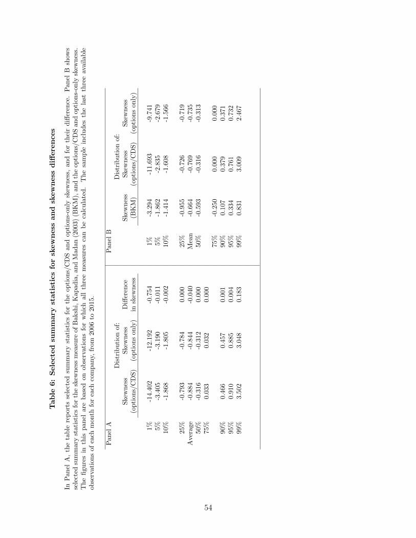
Tab

le6:

Sele

cte

dsu

mm

ary

stati

stic

sfo

rsk

ew

ness

an

dsk

ew

ness

diff

ere

nces

InP

anel

A,

the

tab

lere

por

tsse

lect

edsu

mm

ary

stati

stic

sfo

rth

eop

tion

s/C

DS

an

dop

tion

s-on

lysk

ewn

ess,

an

dfo

rth

eir

diff

eren

ce.

Pan

elB

show

sse

lect

edsu

mm

ary

stat

isti

csfo

rth

esk

ewn

ess

mea

sure

of

Baksh

i,K

ap

ad

ia,

an

dM

ad

an

(2003)

(BK

M),

and

the

op

tion

s/C

DS

an

dop

tion

s-on

lysk

ewn

ess.

Th

efi

gure

sin

this

pan

elar

eb

ased

onob

serv

atio

ns

for

wh

ich

all

thre

em

easu

res

can

be

calc

ula

ted

.T

he

sam

ple

incl

ud

esth

ela

stth

ree

avail

ab

leob

serv

atio

ns

ofea

chm

onth

for

each

com

pan

y,fr

om

2006

to2015.

Pan

elA

Pan

elB

Dis

trib

uti

on

of:

Dis

trib

uti

on

of:

Ske

wn

ess

Ske

wnes

sD

iffer

ence

Ske

wn

ess

Ske

wn

ess

Ske

wn

ess

(op

tion

s/C

DS

)(o

pti

on

son

ly)

insk

ewn

ess

(BK

M)

(op

tion

s/C

DS

)(o

pti

on

son

ly)

1%-1

4.40

2-1

2.1

92

-0.7

54

1%

-3.2

94

-11.6

93

-9.7

41

5%-3

.405

-3.1

90

-0.0

11

5%

-1.8

62

-2.8

35

-2.6

79

10%

-1.8

68-1

.805

-0.0

02

10%

-1.4

14

-1.6

08

-1.5

66

25%

-0.7

93-0

.784

0.0

00

25%

-0.9

55

-0.7

26

-0.7

19

Ave

rage

-0.8

84-0

.844

-0.0

40

Mea

n-0

.664

-0.7

69

-0.7

35

50%

-0.3

16-0

.312

0.0

00

50%

-0.5

93

-0.3

16

-0.3

13

75%

0.03

30.

032

0.0

00

75%

-0.2

50

0.0

00

0.0

00

90%

0.46

60.

457

0.0

01

90%

0.1

07

0.3

79

0.3

71

95%

0.91

00.

885

0.0

04

95%

0.3

34

0.7

61

0.7

32

99%

3.50

23.

048

0.1

83

99%

0.8

31

3.0

09

2.4

67

54

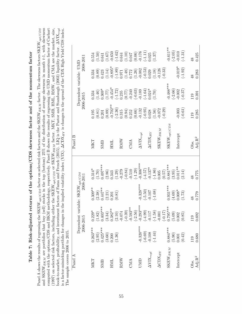
Tab

le7:

Ris

k-a

dju

sted

retu

rns

of

the

op

tion

s/C

DS

skew

ness

facto

ran

dof

the

mom

entu

mfa

cto

r

Pan

elA

show

sth

ere

sult

sof

regr

essi

ng

the

SK

EWopt/CDS

fact

or

on

sele

cted

risk

fact

ors

an

dth

eS

KE

WBKM

fact

or.

Th

esk

ewn

ess

fact

ors

SK

EWopt/CDS

and

SK

EWBKM

are

por

tfol

ios

that

bu

y(s

ell)

stock

sin

the

top

(bott

om

)25%

of

the

dis

trib

uti

on

of

aver

age

skew

nes

sin

month

t-1,

wit

hsk

ewn

ess

com

pu

ted

wit

hth

eop

tion

s/C

DS

and

BK

Mm

ethod

olo

gy,

resp

ecti

vely

.P

an

elB

show

sth

ere

sult

sof

regre

ssin

gth

eU

MD

mom

entu

mfa

ctor

of

Carh

art

(199

7)on

sele

cted

risk

fact

ors,

incl

ud

ing

eith

erth

eS

KE

Wopt/CDS

or

SK

EWBKM

fact

or.

MK

T,

SM

B,

HM

L,

RM

W,

an

dC

MA

are

the

mark

et,

size

,b

ook

-to-

mar

ket,

pro

fita

bil

ity,

and

inve

stm

ent

fact

ors

of

Fam

aan

dF

ren

ch(2

015).

LIQ

isth

eP

ast

or

an

dS

tam

bau

gh

(2003)

liqu

idit

yfa

ctor.

∆V

IXrepl

isa

fact

or-m

imic

kin

gp

ortf

olio

for

chan

ges

inth

eim

pli

edvo

lati

lity

ind

ex(V

IX).

∆C

DXHY

isch

an

ges

inth

esp

read

of

the

CD

XH

igh

-Yie

ldC

DS

ind

ex.

Th

esa

mp

leco

vers

2006

to20

15.

Pan

elA

Pan

elB

Dep

end

ent

vari

able

:S

KE

Wopt/CDS

Dep

end

ent

vari

ab

le:

UM

D20

06-2

015

2008-2

011

2006-2

015

2008-2

011

MK

T0.

263*

**0.

229*

0.3

09**

0.3

14*

MK

T0.1

95

0.3

34

0.3

34

0.5

54

(2.9

5)(1

.82)

(2.3

8)

(1.7

0)

(0.8

1)(1

.46)

(0.8

9)

(1.5

0)

SM

B0.

425*

**0.

403*

**0.4

47**

0.4

97***

SM

B0.2

01

0.3

69*

0.4

23

0.6

41

(3.6

0)(3

.34)

(2.2

1)

(2.8

6)

(0.8

9)(1

.77)

(1.1

4)

(1.6

7)

HM

L0.

200

0.38

2**

0.2

01

0.3

43

HM

L-0

.702

**

-0.4

54*

-0.8

95*

-0.6

50

(1.3

6)(2

.10)

(0.8

1)

(1.2

9)

(-2.3

6)

(-1.7

2)

(-1.8

9)

(-1.6

2)

RM

W-0

.074

-0.2

79

RM

W0.3

15

0.2

35

0.9

71

0.6

44

(-0.

39)

(-0.8

4)

(0.9

4)(0

.77)

(1.4

8)

(1.1

0)

CM

A-0

.593

**-0

.510

CM

A0.2

52

-0.2

40

0.7

72

0.0

47

(-2.

56)

(-1.2

9)

(0.6

6)(-

0.6

3)

(1.2

6)

(0.0

6)

UM

D-0

.320

***

-0.2

93**

*-0

.328***

-0.3

06***

∆V

IXrepl

-0.1

32

-0.1

89

-0.0

82

-0.1

76

(-6.

69)

(-4.

99)

(-5.5

0)

(-4.5

7)

(-0.9

5)

(-1.6

4)

(-0.5

3)

(-1.1

1)

∆V

IXrepl

-0.1

08-0

.117

-0.1

07

-0.1

37*

∆C

DXHY

0.0

28

0.0

24*

0.0

29

0.0

25

(-1.

44)

(-1.

58)

(-1.6

8)

(-1.8

6)

(1.5

6)(1

.70)

(1.1

8)

(1.3

7)

∆C

DXHY

-0.0

010.0

05

SK

EWBKM

-0.0

72

-0.1

26

(-0.

17)

(0.5

7)

(-0.2

9)

(-0.3

3)

SK

EWBKM

0.88

4***

0.79

5***

0.9

31***

0.8

81***

SK

EWopt/CDS

-0.4

88***

-0.6

11**

(5.9

0)(5

.09)

(4.6

9)

(3.9

5)

(-2.6

6)

(-2.0

5)

Inte

rcep

t0.

001

0.00

20.0

08*

0.0

11**

Inte

rcep

t-0

.003

-0.0

02

-0.0

19*

-0.0

10

(0.4

2)(0

.85)

(1.7

3)

(2.1

4)

(-0.6

1)

(-0.3

7)

(-1.9

2)

(-1.3

1)

Ob

s.11

911

948

48

Ob

s.119

119

48

48

Ad

j.R

20.

680

0.69

20.7

79

0.7

75

Ad

j.R

20.2

85

0.3

91

0.2

83

0.4

25

55

Table 8: Time series intercept of the DS factor: full sample

The table reports coefficients, intercepts, t-statistics, number of observations, and adjusted R2s from regres-sions of the DS factor on the listed factors: DSt = α+

∑Ni=1 βif

it + εt. MKT, SMB, HML, RMW, and CMA

are the market, size, book-to-market, profitability, and investment factors of Fama and French (2015). UMDis the Carhart (1997) momentum factor. LT REV and ST REV are the long run and short run reversalsfactors (see, among others, Fama and French, 1996 and Novy-Marx, 2012, and references therein). LIQ is thePastor and Stambaugh (2003) liquidity factor. ∆VIXrepl, ∆VIX2

repl, and VRPrepl are replicating portfoliosfor changes and squared changes in the implied volatility index VIX, and for the variance risk premium ofBollerslev, Tauchen, and Zhou (2009). ∆CDXHY is changes in the spread of the CDX high-yield CDS index.The t-statistics are based on heteroskedasticity-consistent standard errors. ***, **, and * indicate statisticalsignificance at the 1, 5, and 10 % levels, respectively. The sample includes February 2006 to December 2015.

(1) (2) (3) (4) (5) (6) (7)long leg short leg

MKT 0.060 0.081 0.078 0.021 0.071 0.943*** 0.921***(1.23) (1.62) (1.09) (0.35) (0.99) (11.48) (12.12)

SMB -0.016 0.015 -0.004 -0.056 0.000 -0.022 0.034(-0.22) (0.21) (-0.05) (-0.78) (0.00) (-0.22) (0.34)

HML 0.001 0.191 0.202 0.145 0.209 0.114 -0.031(0.01) (1.44) (1.49) (1.16) (1.53) (0.86) (-0.24)

UMD -0.164*** -0.146*** -0.132*** -0.098** -0.138*** -0.075 0.023(-3.42) (-3.72) (-2.64) (-2.10) (-2.78) (-1.37) (0.43)

LIQ 0.045 0.031 0.039 0.030 0.040 -0.000 -0.030(0.82) (0.52) (0.62) (0.50) (0.63) (-0.00) (-0.40)

RMW -0.110 -0.147 -0.089 -0.134 0.167 0.257(-0.79) (-1.14) (-0.73) (-0.97) (1.16) (1.59)

CMA -0.177 -0.141 -0.059 -0.145 0.027 0.085(-1.02) (-0.84) (-0.35) (-0.86) (0.13) (0.40)

LT REV -0.199** -0.241*** -0.184* -0.215** -0.089 0.095(-1.99) (-2.63) (-1.83) (-2.03) (-0.62) (0.76)

ST REV -0.126* -0.135* -0.118* -0.132* 0.029 0.147*(-1.68) (-1.82) (-1.69) (-1.78) (0.37) (1.78)

∆VIXrepl -0.235*** -0.248*** -0.212*** -0.219*** -0.216*** -0.195* 0.025(-4.15) (-3.96) (-3.64) (-4.22) (-3.76) (-1.97) (0.32)

∆VIX2repl 0.132 0.006 0.112 0.330** 0.323***

(0.99) (0.06) (0.91) (2.27) (2.67)VRPrepl -0.061 -0.119 -0.089 -0.062 0.058

(-0.50) (-1.43) (-0.63) (-0.43) (0.40)∆CDXHY 0.001 -0.000 0.000 0.005 0.006

(0.14) (-0.11) (0.08) (1.11) (1.32)SKEWopt/CDS 0.197*** 0.372*** 0.175**

(3.00) (5.63) (2.43)SKEWBKM 0.070

(0.59)

Intercept 0.003* 0.004** 0.004** 0.003** 0.004** 0.003 -0.000(1.86) (2.07) (2.17) (1.98) (2.17) (1.46) (-0.07)

Obs. 119 119 119 119 119 119 119Adj.R2 0.329 0.397 0.389 0.440 0.385 0.904 0.865

56

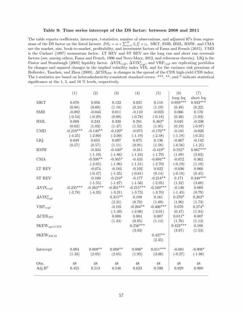
Table 9: Time series intercept of the DS factor: between 2008 and 2011

The table reports coefficients, intercepts, t-statistics, number of observations, and adjusted R2s from regres-sions of the DS factor on the listed factors: DSt = α+

∑Ni=1 βif

it + εt. MKT, SMB, HML, RMW, and CMA

are the market, size, book-to-market, profitability, and investment factors of Fama and French (2015). UMDis the Carhart (1997) momentum factor. LT REV and ST REV are the long run and short run reversalsfactors (see, among others, Fama and French, 1996 and Novy-Marx, 2012, and references therein). LIQ is thePastor and Stambaugh (2003) liquidity factor. ∆VIXrepl, ∆VIX2

repl, and VRPrepl are replicating portfoliosfor changes and squared changes in the implied volatility index VIX, and for the variance risk premium ofBollerslev, Tauchen, and Zhou (2009). ∆CDXHY is changes in the spread of the CDX high-yield CDS index.The t-statistics are based on heteroskedasticity-consistent standard errors. ***, **, and * indicate statisticalsignificance at the 1, 5, and 10 % levels, respectively.

(1) (2) (3) (4) (5) (6) (7)long leg short leg

MKT 0.070 0.056 0.132 0.025 0.118 0.959*** 0.933***(0.88) (0.69) (1.18) (0.24) (1.19) (6.48) (6.22)

SMB -0.082 -0.043 0.011 -0.110 -0.023 0.066 0.176(-0.54) (-0.29) (0.08) (-0.78) (-0.18) (0.36) (1.03)

HML 0.008 0.243 0.338 0.281 0.463* 0.045 -0.236(0.03) (1.03) (1.47) (1.52) (1.95) (0.19) (-0.97)

UMD -0.210*** -0.140** -0.129* -0.075 -0.170** -0.101 -0.026(-4.25) (-2.60) (-2.00) (-1.19) (-2.48) (-1.18) (-0.35)

LIQ 0.049 0.055 0.097 0.075 0.136 -0.067 -0.142(0.57) (0.57) (1.11) (0.91) (1.58) (-0.56) (-1.25)

RMW -0.334 -0.440* -0.311 -0.419* 0.555* 0.867***(-1.19) (-1.86) (-1.24) (-1.79) (1.89) (3.63)

CMA -0.508** -0.565* -0.433 -0.694** -0.072 0.362(-2.05) (-1.96) (-1.51) (-2.70) (-0.19) (1.18)

LT REV -0.074 -0.183 -0.102 0.022 -0.036 0.066(-0.47) (-1.35) (-0.61) (0.14) (-0.18) (0.45)

ST REV -0.169 -0.210* -0.177 -0.218** 0.171 0.348***(-1.55) (-1.87) (-1.56) (-2.05) (1.32) (3.60)

∆VIXrepl -0.235*** -0.263*** -0.201*** -0.215*** -0.249*** -0.146 0.069(-3.78) (-4.33) (-3.31) (-3.73) (-3.70) (-1.45) (0.79)

∆VIX2repl 0.315** 0.109 0.161 0.370* 0.262*

(2.31) (0.70) (1.09) (1.90) (1.73)VRPrepl -0.191 -0.204** -0.406*** 0.070 0.274*

(-1.49) (-2.06) (-3.01) (0.47) (1.94)∆CDXHY 0.008 0.004 0.007 0.011* 0.007

(1.24) (0.85) (1.14) (1.76) (1.13)SKEWopt/CDS 0.256*** 0.423*** 0.166

(3.03) (3.87) (1.53)SKEWBKM 0.427**

(2.35)

Intercept 0.004 0.008** 0.008** 0.006* 0.011*** -0.001 -0.008*(1.33) (2.05) (2.05) (1.95) (3.06) (-0.27) (-1.98)

Obs. 48 48 48 48 48 48 48Adj.R2 0.455 0.513 0.546 0.623 0.590 0.929 0.908

57

Table 10: Fama-MacBeth regressions (1/2)

The table shows the second-stage coefficients from Fama and MacBeth (1973) regressions. The test assetsare 25 book-to-market/size portfolios replicated using the stocks with available volatility spreads (Bali andHovakimian, 2009) and smirks (Xing, Zhang, and Zhao, 2010), and 10 decile portfolios based on the DSmeasure in month t-1. The characteristics (portfolios averages in month t-1), are idiosyncratic volatility (Ang,Hodrick, Xing, and Zhang, 2006) (ivol), average 5-year CDS log-spread (sprd5yr), hybrid tail covariance (Bali,Cakici, and Whitelaw, 2014) (covtail), changes in call/put implied volatility of An, Ang, Bali, and Cakici(2014) (∆cvol and ∆pvol), and volatility spreads (vspread) and smirks (smirk). Adj.R2

cr is the average adj.R2 of the second-stage regressions. The sample covers February 2006 to December 2015.

2006-2015 2008-2011(1) (2) (3) (4) (5) (6) (7) (8)

λ0 0.034 0.023 0.027 0.019 0.003 0.004 0.023 0.020(1.37) (0.94) (1.61) (1.16) (0.07) (0.10) (0.87) (0.63)

ivol -0.251* -0.215* -0.154* -0.153* -0.293 -0.168 -0.285** -0.234(-1.83) (-1.77) (-1.71) (-1.70) (-1.35) (-0.93) (-2.17) (-1.58)

sprd5yr 0.354 0.235 0.248 0.133 -0.015 0.058 0.259 0.170(1.04) (0.72) (0.94) (0.52) (-0.03) (0.11) (0.72) (0.39)

covtail -0.007 -0.007 -0.010 -0.011* -0.012* -0.012* -0.010** -0.008(-0.96) (-0.97) (-1.55) (-1.87) (-1.93) (-1.99) (-2.08) (-1.18)

∆cvol 0.098 0.100 0.121 0.215 0.194* 0.214(0.93) (1.13) (1.31) (1.51) (1.85) (1.51)

∆pvol -0.027 -0.049 -0.066 -0.223 -0.200* -0.206(-0.27) (-0.58) (-0.77) (-1.47) (-1.78) (-1.39)

vspread 0.034 0.028 0.008 0.007(0.80) (0.69) (0.10) (0.09)

smirk 0.079 0.080 0.205* 0.139(0.92) (0.94) (1.94) (1.40)

MKT 0.003 0.007 0.002 0.005 0.012 0.013 0.010 0.005(0.37) (0.78) (0.25) (0.56) (0.98) (1.14) (0.79) (0.39)

SMB 0.002 0.002 0.002 0.002 0.002 -0.001 0.001 -0.001(0.46) (0.64) (0.46) (0.59) (0.43) (-0.20) (0.33) (-0.33)

HML -0.007 -0.008 -0.005 -0.004 0.006 0.004 0.003 0.005(-1.36) (-1.62) (-1.11) (-0.88) (0.77) (0.53) (0.44) (0.64)

UMD -0.002 0.004 -0.004 -0.006 -0.006 0.007 -0.002 -0.001(-0.20) (0.31) (-0.40) (-0.59) (-0.27) (0.32) (-0.13) (-0.09)

LT REV -0.006* -0.005 -0.003 -0.003 -0.001 0.002 0.001 0.001(-1.71) (-1.32) (-1.03) (-0.77) (-0.18) (0.26) (0.21) (0.10)

ST REV -0.008 -0.009 -0.008 -0.009 -0.003 -0.005 0.000 -0.002(-1.26) (-1.21) (-1.11) (-1.28) (-0.19) (-0.31) (-0.02) (-0.12)

LIQ 0.000 0.000 0.000 0.000 0.012 0.010 0.009 0.005(-0.04) (0.00) (0.04) (0.03) (0.65) (0.54) (0.55) (0.31)

∆VIX 0.001 0.001 0.004 -0.002 -0.020 -0.017 -0.015 -0.016(0.07) (0.11) (0.34) (-0.19) (-1.44) (-1.20) (-1.06) (-1.06)

∆VIX2 0.003* 0.003* 0.002 0.002 0.003 0.003 0.002 0.003(1.85) (1.84) (1.63) (1.65) (1.27) (1.25) (1.00) (1.24)

SKEWopt/CDS 0.008 0.007 0.007 0.017 0.012 0.013(1.08) (0.97) (1.09) (1.23) (0.96) (1.12)

SKEWBKM 0.002 -0.001(0.46) (-0.16)

DS 0.005** 0.005* 0.004** 0.005** 0.011* 0.010 0.010* 0.010*(2.01) (1.82) (2.01) (2.22) (1.99) (1.64) (1.90) (1.92)

Adj.R2cr 0.529 0.497 0.498 0.489 0.653 0.644 0.633 0.626

58

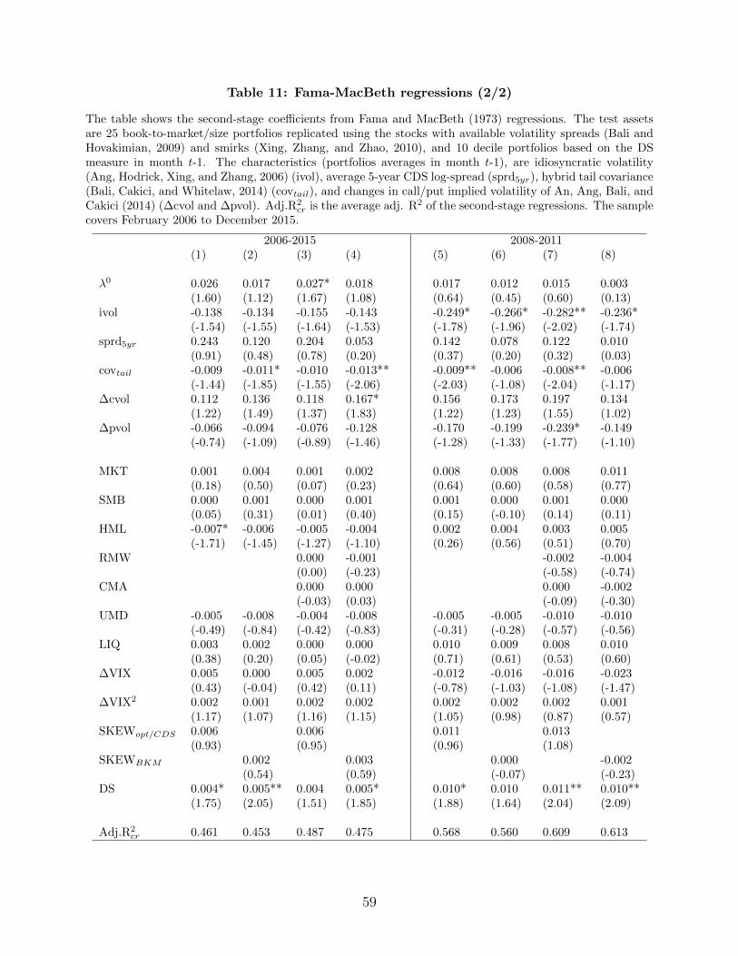
Table 11: Fama-MacBeth regressions (2/2)

The table shows the second-stage coefficients from Fama and MacBeth (1973) regressions. The test assetsare 25 book-to-market/size portfolios replicated using the stocks with available volatility spreads (Bali andHovakimian, 2009) and smirks (Xing, Zhang, and Zhao, 2010), and 10 decile portfolios based on the DSmeasure in month t-1. The characteristics (portfolios averages in month t-1), are idiosyncratic volatility(Ang, Hodrick, Xing, and Zhang, 2006) (ivol), average 5-year CDS log-spread (sprd5yr), hybrid tail covariance(Bali, Cakici, and Whitelaw, 2014) (covtail), and changes in call/put implied volatility of An, Ang, Bali, andCakici (2014) (∆cvol and ∆pvol). Adj.R2

cr is the average adj. R2 of the second-stage regressions. The samplecovers February 2006 to December 2015.

2006-2015 2008-2011(1) (2) (3) (4) (5) (6) (7) (8)

λ0 0.026 0.017 0.027* 0.018 0.017 0.012 0.015 0.003(1.60) (1.12) (1.67) (1.08) (0.64) (0.45) (0.60) (0.13)

ivol -0.138 -0.134 -0.155 -0.143 -0.249* -0.266* -0.282** -0.236*(-1.54) (-1.55) (-1.64) (-1.53) (-1.78) (-1.96) (-2.02) (-1.74)

sprd5yr 0.243 0.120 0.204 0.053 0.142 0.078 0.122 0.010(0.91) (0.48) (0.78) (0.20) (0.37) (0.20) (0.32) (0.03)

covtail -0.009 -0.011* -0.010 -0.013** -0.009** -0.006 -0.008** -0.006(-1.44) (-1.85) (-1.55) (-2.06) (-2.03) (-1.08) (-2.04) (-1.17)

∆cvol 0.112 0.136 0.118 0.167* 0.156 0.173 0.197 0.134(1.22) (1.49) (1.37) (1.83) (1.22) (1.23) (1.55) (1.02)

∆pvol -0.066 -0.094 -0.076 -0.128 -0.170 -0.199 -0.239* -0.149(-0.74) (-1.09) (-0.89) (-1.46) (-1.28) (-1.33) (-1.77) (-1.10)

MKT 0.001 0.004 0.001 0.002 0.008 0.008 0.008 0.011(0.18) (0.50) (0.07) (0.23) (0.64) (0.60) (0.58) (0.77)

SMB 0.000 0.001 0.000 0.001 0.001 0.000 0.001 0.000(0.05) (0.31) (0.01) (0.40) (0.15) (-0.10) (0.14) (0.11)

HML -0.007* -0.006 -0.005 -0.004 0.002 0.004 0.003 0.005(-1.71) (-1.45) (-1.27) (-1.10) (0.26) (0.56) (0.51) (0.70)

RMW 0.000 -0.001 -0.002 -0.004(0.00) (-0.23) (-0.58) (-0.74)

CMA 0.000 0.000 0.000 -0.002(-0.03) (0.03) (-0.09) (-0.30)

UMD -0.005 -0.008 -0.004 -0.008 -0.005 -0.005 -0.010 -0.010(-0.49) (-0.84) (-0.42) (-0.83) (-0.31) (-0.28) (-0.57) (-0.56)

LIQ 0.003 0.002 0.000 0.000 0.010 0.009 0.008 0.010(0.38) (0.20) (0.05) (-0.02) (0.71) (0.61) (0.53) (0.60)

∆VIX 0.005 0.000 0.005 0.002 -0.012 -0.016 -0.016 -0.023(0.43) (-0.04) (0.42) (0.11) (-0.78) (-1.03) (-1.08) (-1.47)

∆VIX2 0.002 0.001 0.002 0.002 0.002 0.002 0.002 0.001(1.17) (1.07) (1.16) (1.15) (1.05) (0.98) (0.87) (0.57)

SKEWopt/CDS 0.006 0.006 0.011 0.013(0.93) (0.95) (0.96) (1.08)

SKEWBKM 0.002 0.003 0.000 -0.002(0.54) (0.59) (-0.07) (-0.23)

DS 0.004* 0.005** 0.004 0.005* 0.010* 0.010 0.011** 0.010**(1.75) (2.05) (1.51) (1.85) (1.88) (1.64) (2.04) (2.09)

Adj.R2cr 0.461 0.453 0.487 0.475 0.568 0.560 0.609 0.613

59

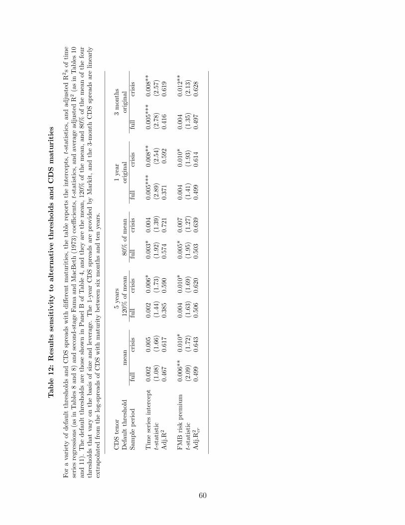
Tab

le12:

Resu

lts

sen

siti

vit

yto

alt

ern

ati

ve

thre

shold

san

dC

DS

matu

riti

es

For

ava

riet

yof

def

ault

thre

shol

ds

and

CD

Ssp

read

sw

ith

diff

eren

tm

atu

riti

es,

the

tab

lere

port

sth

ein

terc

epts

,t-

stati

stic

s,an

dad

just

edR

2s

of

tim

ese

ries

regr

essi

ons

(as

inT

able

s8

and

8)an

dse

con

d-s

tage

Fam

aan

dM

acB

eth

(1973)

coeffi

cien

ts,t-

stati

stic

s,an

dav

erage

ad

just

edR

2(a

sin

Tab

les

10

and

11).

Th

ed

efau

ltth

resh

old

sar

eth

ose

show

nin

Pan

elB

of

Tab

le4,

an

dth

eyare

the

mea

n,

120%

of

the

mea

n,

an

d80%

of

the

mea

nof

the

fou

rth

resh

old

sth

atva

ryon

the

bas

isof

size

and

leve

rage.

Th

e1-y

ear

CD

Ssp

read

sare

pro

vid

edby

Mar

kit

,and

the

3-m

onth

CD

Ssp

read

sare

linea

rly

extr

apol

ated

from

the

log-

spre

ads

ofC

DS

wit

hm

atu

rity

bet

wee

nsi

xm

onth

san

dte

nye

ars

.

CD

Ste

nor

5ye

ars

1ye

ar

3m

onth

sD

efau

ltth

resh

old

mea

n120%

of

mea

n80%

of

mea

nori

gin

al

ori

gin

al

Sam

ple

per

iod

full

cris

isfu

llcr

isis

full

cris

isfu

llcr

isis

full

cris

is

Tim

ese

ries

inte

rcep

t0.

002

0.00

50.0

02

0.0

06*

0.0

03*

0.0

04

0.0

05*

**

0.0

08**

0.0

05***

0.0

08**

t-st

atis

tic

(1.0

8)(1

.66)

(1.4

4)

(1.7

3)

(1.9

2)

(1.3

9)

(2.8

9)(2

.54)

(2.7

8)

(2.5

7)

Ad

j.R

20.

467

0.61

70.3

85

0.5

90

0.5

74

0.7

21

0.3

71

0.5

92

0.4

16

0.6

19

FM

Bri

skp

rem

ium

0.00

6**

0.01

0*0.0

04

0.0

10*

0.0

05*

0.0

07

0.0

04

0.0

10*

0.0

04

0.0

12**

t-st

atis

tic

(2.0

9)(1

.72)

(1.6

3)

(1.6

9)

(1.9

5)

(1.2

7)

(1.4

1)

(1.9

3)

(1.3

5)

(2.1

3)

Ad

j.R

2 cr

0.49

90.

643

0.5

06

0.6

20

0.5

03

0.6

39

0.4

99

0.6

14

0.4

97

0.6

28

60