Embed Size (px)
Citation preview

Firm Sorting and Agglomeration
Cecile Gaubert∗
Department of Economics, Princeton University
JOB MARKET PAPER
Abstract
The distribution of firms in space is far from uniform. Some locations host the most produc-tive large firms, while others barely attract any. In this paper, I study the sorting of het-erogeneous firms across locations and analyze policies designed to attract firms to particularregions (place-based policies). I first propose a theory of the distribution of heterogeneousfirms in a variety of sectors across cities. Aggregate TFP and welfare depend on the extentof agglomeration externalities produced in cities and on how heterogeneous firms sort acrossthem. The distribution of city sizes and the sorting patterns of firms are uniquely determinedin equilibrium. This allows me to structurally estimate the model, using French firm-leveldata. I find that nearly two thirds of the observed productivity advantage of large cities isdue to firm sorting. I use the estimated model to quantify the general equilibrium effects ofplace-based policies. I find that policies that decrease local congestion lead to a new spa-tial equilibrium with higher aggregate TFP and welfare. In contrast, policies that subsidizeunder-developed areas have negative aggregate effects.
∗[email protected]. I am extremely grateful to Esteban Rossi-Hansberg, Steve Redding and GeneGrossman for their continuous guidance and support. I also thank Treb Allen, Costas Arkolakis, Thomas Chaney,Jan De Loecker, Oleg Itskhoki, Eduardo Morales, David Nagy, Felix Tintelnot and John Vogel for helpful discussionand comments. Financial support from the International Economics Section at Princeton University is gratefullyacknowledged.
1

1 Introduction
The distribution of firms in space is far from uniform. Some locations host the most productive
large firms, while others barely attract any. Recognizing the key role played by firms in the devel-
opment of local activity, governments offer financial incentives to attract firms to specific areas.
Such interventions aim, in general, to reduce spatial disparities and to increase welfare by fostering
local agglomeration externalities. In practice, though, positive local impacts may be counterbal-
anced by undesirable effects in other regions. In addition, spatial disparities could be reinforced if
subsidies attract low-productivity firms while leaving high-productivity ones in booming regions.
To understand these effects, I propose a theory of the distribution of heterogeneous firms in a
variety of sectors across cities. The model has a unique equilibrium, which is affected by the
implementation of these place-based policies. This allows me to conduct a counterfactual policy
analysis and to quantify their impact in terms of aggregate productivity and welfare.
Place-based policies are pervasive. Kline and Moretti (2013) report that an estimated 95 billion
dollars are spent annually in the United States to attract firms to certain locations. Massive
subsidies are targeted to individual firms in a nationwide competition to attract plants.1 Federal
programs provide generous tax breaks in an effort to attract firms to less developed areas, as
analyzed most recently by Busso et al. (2013). The European Union regulates these aids and
reports a yearly figure of 15 billion euros.2 In a broader sense, place-based policies also encompass
regulations that impact the growth of cities, such as zoning regulations or restrictions on the height
of buildings. I analyze the impact of both types of policies in the light of my framework.
To analyze the long-run impact of these policies, one needs to understand how heterogeneous
firms react to them and how targeted cities grow or shrink as a result. I develop a model that is
uniquely suited to answering these questions. Heterogeneous firms sort across cities. Cities are
endogenously impacted by this sorting. They grow when firms choose to locate there and increase
the local labor demand. Since firms’ location choices are distorted by local policies, cities are,
in turn, endogenously affected. Importantly, the model admits a unique equilibrium, which is
impacted by local policies. The model captures several forces. Cities are ex ante identical. They
are the locus of intangible agglomeration externalities such as thick labor markets or knowledge
spillovers (Duranton and Puga (2003)). The sorting of firms into cities of different sizes is driven
1Examples abound and are compiled in Story (2012). Recent examples include Apple who obtained a reported88 million dollars in tax cuts to locate a data center in Reno, Nevada, Caterpillar with a reported 77 million dollarsincentives to build a plant in Georgia, or Boeing getting a 120 million dollars subsidy from South Carolina toexpand its operations in Charleston.
2In contrast to the United States, the European Union regulates the amount and geographical scope of theseaids. They are restricted to less advantaged regions. Both in Europe and in the US, there exists a wider range ofpolicies that are designed with spatial impact in mind but are not accounted for in these figures, such as the designof local tax reporting for multi-location firms. Bartik (2004) reports a taxonomy of such policies.
2

by a trade-off between gains in productivity, through local externalities, and higher labor costs.
I assume that more efficient firms benefit relatively more from local externalities. This generates
positive assortative matching: more efficient firms locate in larger cities, reinforcing their initial
edge. A class of city developers compete to attract firms to their city. They act as a coordinating
device in the economy, leading to a unique spatial equilibrium.
Using firm-level data, I show that the model is able to reproduce salient features of the French
economy. First, in the model, initial differences in productivity between firms induce sorting across
city sizes. This, in turn, reinforces firm heterogeneity, as firms in large cities benefit from stronger
agglomeration forces. The resulting firm-size distribution is more thick-tailed for sectors that tend
to locate in larger cities. Second, across sectors, firm sorting is shaped by the intensity of input
use. In labor-intensive sectors, firms locate more in small cities where wages are lower. Third,
within sectors, firms have higher revenues in larger cities. They may have lower employment,
though, since they face higher labor costs. I show that these outcomes of the model are broadly
consistent with stylized facts about French firms.
I structurally estimate the model. This structure is needed to quantify the impact of place-based
policies on the spatial equilibrium, absent a real-life counterfactual. The structural estimation
recovers a model-based estimate of the shape of agglomeration externalities. It allows me to
disentangle the roles played by agglomeration forces on the one hand, and firm sorting on the
other hand, in shaping productivity gains associated with city size. I estimate that nearly two
thirds of the measured productivity advantage of large cities comes from the sorting of firms based
on their efficiency. The magnitude of the agglomeration economies I estimate are in line with
existing estimates in the literature as reported by Rosenthal and Strange (2004).
Finally, I simulate the new spatial equilibrium that results from two policies: a tax-relief scheme
targeted at firms locating in smaller cities, and the removal of regulations that hamper city growth,
such as zoning or building-height regulations, as advocated by Glaeser and Gottlieb (2008). Firms
make different location choices as a result, which modifies local labor demand and in equilibrium
impacts the city-size distribution. The productive efficiency of the new equilibrium depends in
particular on the new city-size distribution: it drives the extent of agglomeration externalities
leveraged by firms in the economy. I find that a policy that subsidizes less productive areas has
negative aggregate effects on TFP and welfare. In contrast, a policy that favors the growth of
cities leads to a new spatial equilibrium that is significantly more productive, by endogenously
creating agglomeration externalities and reducing the impact of market failures.
The paper is related to several strands of the literature. The main contribution of the paper is to
propose a model of spatial equilibrium that is well suited to the analysis of place-based policies,
since it features freely mobile, heterogeneous firms and endogenous city sizes, and has a unique
3

equilibrium. The literature that studies systems of cities, pioneered by Henderson (1974), has tra-
ditionally focused on homogenous firms. Recent contributions have introduced richer heterogeneity
in the spatial setting.3 In a seminal contribution, Behrens et al. (2010) study the spatial sorting
of entrepreneurs who produce non-tradable intermediates. I study the polar case of producers
of perfectly tradable goods. An important difference for policy analysis is the uniqueness of the
equilibrium I obtain here. Another closely related strand of the literature (Eeckhout et al. (2010),
Davis and Dingel (2012) and Davis and Dingel (2013)) studies the spatial sorting of workers who
differ in skill level, to shed light on patterns of wage inequality and on the spatial distribution of
skills. My paper uses similar conceptual tools, borrowed from the assignment literature, to focus
on how firms sort and impact local labor demand, motivated by the fact that firms are directly
targeted by place-based policies.4
Second, the model shows novel theoretical and empirical evidence of a link between the geo-
graphical pattern of economic activity and the sectoral firm-size distribution. It contributes to
the literature that aims to explain the determinants of firm-size distribution by exploiting cross-
sectoral heterogeneity. Rossi-Hansberg and Wright (2007a) focus on the role of decreasing returns
to scale in determining the shape of the establishment-size distribution, while di Giovanni et al.
(2011) consider the role played by endogenous selection into exporting. I focus instead on the role
played by location choice. The model also contributes to the literature on city-size distribution.
City-size distribution is traditionally explained by random growth models, as in Gabaix (1999)
and Eeckhout (2004), for example. Here, as in Behrens et al. (2010), the distribution of city sizes
is endogenous to the sorting of heterogeneous firms in a static spatial equilibrium, since cities are
the collection of the labor force employed by local firms. The city-size distribution is shaped by
properties of the firm-size distribution.
As in Desmet and Rossi-Hansberg (2013) and Behrens et al. (2013), I use structural estimation
of a model of a system of cities to assess the welfare implications of the spatial equilibrium. The
focus of the analysis is different, since they do not explicitly account for sorting by heterogeneous
firms. The paper also contributes to the literature that measures agglomeration externalities, as
reviewed in Rosenthal and Strange (2004). Most analyses do not take into account the sorting
of heterogeneous agents, workers or firms, across locations. A notable exception is Combes et
al. (2008), who use detailed data on workers characteristics to control for worker heterogeneity
and sorting in a reduced form analysis. I use a structural approach to explicitly account for the
3Early studies of heterogeneous firms in the spatial context include Nocke (2006) and Baldwin and Okubo (2006).They predict that more productive firms self-select in larger markets. These results are obtained in a setting wherethe size of regions is fixed and exogenously given. In contrast, I focus on how local policies endogenously changethe spatial equilibrium, including city sizes themselves, as they attain their objective to see targeted cities grow.
4The model borrows insights from the assignment model literature, such as Costinot and Vogel (2010), and inparticular Eeckhout and Kircher (2012) and Sampson (forthcoming), who focus on heterogeneous firms matchingwith heterogeneous workers. Here, firms match with heterogeneous city sizes.
4

sorting of firms. Combes et al. (2012) also emphasize the heterogeneous effect of agglomeration
externalities on heterogeneous firms. They show that the most efficient firms are disproportionally
more efficient in large cities, indicating potential complementarities between firm productivity
and city size. Their analysis is based on a model without firm location choice, in contrast to the
approach I take.
Finally, the counterfactual policy analysis offers a complementary approach to research that as-
sesses the impact of specific place-based policies (see, for example, Busso et al. (2013) for the
US, Mayer et al. (2012) for France and Criscuolo et al. (2012) for the UK). The literature has
traditionally focused on estimating the local effects of these policies. A notable exception is Kline
and Moretti (2013), who develop a methodology to estimate their aggregate effects.5 For the
policy they consider, they estimate that positive local effects are offset by losses in other parts
of the country. My approach is similar in spirit, with the difference that I account explicitly for
firm sorting. I find a negative aggregate effect of policies targeting the smallest cities. Finally,
Glaeser and Gottlieb (2008) study theoretically the economic impact of place-based policies. My
analysis brings in heterogeneous firms and the general equilibrium effect of place-based policies on
the productive efficiency of the country.
The paper is organized as follows. Section 2 presents the model and its predictions. Section
3 details the empirical analysis. I show salient features from French firm-level data that are
consistent with the forces at play in the model. I then structurally estimate the model using
indirect inference. In section 4, I conduct a counterfactual analysis using the estimated model.
Section 5 concludes.
2 A Model of the Location Choice of Heterogeneous Firms
Consider an economy in which production takes place in locations that I call cities. The economy
is composed of a variety of sectors. Within sectors, firms are heterogeneous in productivity. They
produce, in cities, using local labor and traded capital. Non-market interactions within cities
give rise to positive agglomeration externalities. I assume that they have heterogeneous effects on
firms, in the sense that more efficient firms are more able to leverage local externalities. Firms’
choice of city results from a trade-off between the strength of local externalities, the local level
of input prices and, possibly, the existence of local subsidies. Heterogeneous firms face different
incentives, which yields heterogeneity in their choice. I follow Henderson (1974) and postulate
the existence of a class of city developers. In each potential city site, a developer represents local
5Albouy (2012) focuses on a related question. He argues that federal taxes impose a de facto unequal geographicburden since they do not account for differences in local cost of living, and estimates he the corresponding welfarecost.
5

landowners and competes against other sites to attract firms. City developers play a coordination
role in the creation of cities, which leads to a unique equilibrium of the economy. The model
describes a long-run steady state of the economy and abstracts from dynamics.
2.1 Set-up and agents’ problem
2.1.1 Cities
Each potential city site has a given stock of land, normalized to 1. Sites are identical ex-ante.
Cities emerge endogenously on these sites, potentially with different population levels L. In
what follows, I index cities and all the relevant city-level parameters by city size L. City size is
sufficient to characterize all the economic forces at play, in the tradition of models of systems of
cities pioneered by Henderson (1974). In particular the distance between two cities plays no role
as goods produced in the economy are either freely traded between cities within the country, or
are, in the case of housing, non tradable.
Land is used to build housing, which is divisible and consumed by workers. Atomistic landown-
ers construct housing h by combining their land s with local labor `, according to the housing
production function
h = sb( `
1− b)1−b
. (1)
The land-use intensity b governs the amount of housing that can be produced with a given stock
of land. Lowering b increases the housing supply in a city where the stock of land is fixed.
This parameter summarizes the technological and regulatory constraints on housing supply in a
city. In the policy experiments, I analyze how it impacts productivity and welfare in the spatial
equilibrium.
Landowners compete in the housing market, taking both the housing price pH(L) and the local
wage w(L) as given. Since there is a fixed supply of land in the city, the housing supply equation
is
H(L) =(pH(L)
w(L)
) 1−bb , (2)
where H(L) is the total quantity of housing supplied in a city of size L.
2.1.2 Workers
Set-up There is a mass N0 of identical workers. Each worker is endowed with one unit of labor.
A worker lives in the city of his choosing, consumes a bundle of traded goods and housing, and is
6

paid the local wage w(L). Workers’ utility is
U =
(c
η
)η(h
1− η
)1−η
, (3)
where h denotes housing and c is a Cobb-Douglas bundle of goods across S sectors of the economy
defined as
c =
j=S∏j=1
cξjj , with
j=S∑j=1
ξj = 1.
Within a sector j, consumers choose varieties according to the CES aggregator
cj =
[ ∫cj(i)
σj−1
σj di
] σjσj−1
.
I denote by P the aggregate price index for the composite good c. Since goods are freely tradable,
the price index is the same across cities. Workers are perfectly mobile and ex ante identical.
Workers’ problem Workers in city L consume c(L) units of the good and h(L) units of housing
to maximize their utility (3), under the budget constraint
P c(L) + pH(L)h(L) = w(L).
As a result, the aggregate local demand for housing is
H(L) =(1− η)w(L)L
pH(L). (4)
The local housing market clears. Equations (2) and (4) pin down prices and quantities of housing
produced.6 The quantity of housing consumed by each worker in city L is
h(L) = (1− η)1−b L−b. (5)
Housing consumption is lower in more populous cities because cities are constrained in space.
This congestion force counterbalances the agglomeration-inducing effects of positive production
externalities in cities and prevents the economy from complete agglomeration into one city.
Since workers are freely mobile, their utility must be equalized in equilibrium across all inhabited
locations to a level U . In equilibrium, wages must increase with city size to compensate workers
6Appendix A gives the equilibrium housing prices and labor hired.
7

for congestion costs, according to
w(L) = w((1− η)L) b1−ηη , (6)
where w = U1η P is an economy-wide constant to be determined in the general equilibrium.
2.1.3 Firms
Production The economy consists of many sectors that manufacture differentiated tradable
products. Firms have the same factor intensities within their sectors but differ in productivity.
Firms produce varieties using two factors of production that have the following key characteristics.
One has a price that increases with city size; the other has a constant price across cities. For
simplicity, I consider only one factor whose price depends on city size: labor. In particular, I do
not consider land directly in the firm production function. I call the other factor capital, as a
shorthand for freely tradable inputs. Capital is provided competitively by absentee capitalists.
The price of capital is fixed exogenously in international markets, and the stock of capital in the
country adjusts to the demand of firms.
Firms differ exogenously in efficiency z. A firm of efficiency z in sector j and city of size L produces
output according to the following Cobb-Douglas production function
yj(z, L) = ψ(z, L, sj) kαj `1−αj ,
where ` and k denote labor and capital inputs, αj is the capital intensity of firms in sector j and
ψ(z, L, sj) is a firm-specific Hicks-neutral productivity shifter, as detailed below. It is determined
by the firm’s ‘raw’ efficiency, the extent of the local agglomeration externalities and a sector-specific
parameter sj.
Firms engage in monopolistic competition. Varieties produced by firms are freely tradable across
space: there is a sectoral price index that is constant through space. Firms take it as given.
What matters for location choice is the trade-off between production externalities and costs of
production. The relative input price varies with city size. Wages increase with L (equation (6)),
whereas capital has a uniform price. Therefore, the factor intensity of a firm shapes, in part, its
location decision. A more labor-intensive firm faces, all else equal, a greater incentive to locate in
a smaller city where wages are lower.
Productivity and agglomeration The productivity of a firm ψ(z, L, sj) depends on its own
‘raw’ efficiency z, on local agglomeration externalities that increase with city size L, and on a
sector-specific parameter sj. I explain the roles of these parameters in turn.
8
A key assumption of the model is that ψ exhibits a strong complementarity between local external-
ities and the efficiency of the firm. Firms that are more efficient at producing are also more efficient
at leveraging local agglomeration externalities, such as knowledge spillovers or labor-market pool-
ing. The empirical literature offers some suggestive evidence pointing to such complementarity
between firm efficiency and agglomeration externalities. Arzaghi and Henderson (2008) present
an empirical study of the advertising industry. They measure the benefit agencies derive from
interactions in local networks and provide evidence that agencies that were larger in the first place
are more willing than smaller ones to pay higher rents in order to have access to a better local
network. Combes et al. (2012) study a wide set of French industries and provide suggestive evi-
dence that more efficient firms are disproportionately more productive in larger cities, pointing to
such a complementarity as a potential explanation for this fact. Finally, in Section 3, I present a
set of stylized facts on French firms’ location and production patterns. They are consistent with
sorting, a consequence of the assumed complementarity.
Knowledge spillovers can arguably exhibit this type of complementarity. More efficient firms can
better leverage the local information they obtain. A similar idea, though for individual agents,
is provided by Davis and Dingel (2012). In their model, more able individuals optimally spend
less time producing and more time leveraging local knowledge, which increases their productivity,
leading to such a complementarity. In Appendix B, I extend this idea to the set-up of my model
where workers are hired to produce the blueprint of the firm. The firm can have workers work
at the plant or spend time improving the blueprint by leveraging local information, e.g., on pro-
duction processes or product appeal. It is optimal for more efficient firms to encourage workers
to spend more time discovering local ideas. As a result, the productivity of the firm exhibits
complementarity between city size and the firm’s own efficiency.7
In what follows, I remain agnostic on the source of agglomeration externalities and their spe-
cific functional form. This allows me to highlight the generic features of an economy with such
complementarities. I let the productivity ψ(z, L, s) have the following properties:
Assumption A ψ(z, L, s) is log-supermodular in city size L, firm raw efficiency z and sectoral
characteristic s, and is twice differentiable. That is,
∂2log ψ(z, L, s)
∂L∂z≥ 0,
∂2log ψ(z, L, s)
∂L∂s≥ 0, and
∂2log ψ(z, L, s)
∂z∂s≥ 0.
I introduce a sector-specific parameter sj that allows sectors to vary in the way they benefit
from local urbanization externalities. Rosenthal and Strange (2004) note that empirical studies
7The productivity function is log-supermodular in firm efficiency and city size.
9

suggest that the force and scope of agglomeration externalities vary across industries. More specif-
ically, Audretsch and Feldman (1996) suggest that the benefits from agglomeration externalities
are shaped by an industry’s life-cycle and that highly innovative sectors benefit more strongly
from local externalities than mature industries. I index industries such that, in high s sectors,
firms benefit from stronger agglomeration forces, for a given city size.8 In the estimation of the
model, I allow for parameter values that shut down the heterogeneous effect between agglomera-
tion externalities and firm efficiency. The specification I retain for ψ nests the typical specification
considered in the literature, where only agglomeration forces of the form ψ = zLs are at play.9
Finally, I restrict the analysis to productivity functions ψ(z, L, s) for which the firms’ problem is
well defined and concave, absent any local subsidies, for all firms. In other words, I assume that the
positive effects of agglomeration externalities are not too strong compared to the congestion forces.
In particular, given that the congestion forces increase with city size with a constant elasticity,
agglomeration externalities must have decreasing elasticity to city size to prevent a degenerate
outcome with complete agglomeration of firms in the largest city.
Entry and location choice There is an infinite supply of potential entrants who can enter the
sector of their choosing. Firms pay a sunk cost fEj in terms of the final good to enter sector j,
then draw a raw efficiency level z from a distribution Fj(.). I assume that this distribution has
convex support. This assumption is made for tractability; the results carry through without it,
although the notation is more cumbersome. Once firms discover their raw efficiency, they choose
the size of the city where they want to produce.10
Firms’ problem A firms’ choice of city size is influenced by three factors. First, relative input
prices vary by city size. Second, firm productivity increases with city size, through greater ag-
glomeration externalities. Third, local city developers compete to attract firms to their cities by
subsidizing profits at rate Tj(L), which varies by city-size and sector.11
The firm’s problem can be solved recursively. For a given city size, the problem of the firm is to
hire labor and capital and set prices to maximize profits, taking as given the size of the city (and
8In addition, I assume that ∂2log ψ(z,L,s)∂z∂s is non-negative. For any city size L, the elasticity of firm productivity
to its initial efficiency is either equal across sectors, or larger in high s sectors.9In that case ∂2log ψ(z,L,s)
∂L∂z = 0, ∂2log ψ(z,L,s)
∂s∂z = 0 and ∂2log ψ(z,L,s)∂L∂s > 0.
10Contrary to the setting in Melitz (2003), the model abstracts from any selection of firms at entry, since there isno fixed cost to produce. I focus instead on where firms decide to produce once they discover their efficiency, andhow this shapes the spatial equilibrium of the economy. That is, rather than selection on entry, I focus on selectionon city size.
11The subsidy offered by city developers Tj(L) may in principle differ across cities for cities of the same size.As I show in the next section, this is not the case in equilibrium. Anticipating this, I abstract from introducingcumbersome notation denoting different cities of the same size.
10

hence the size of the externality term), input prices, and subsidies. Then, firms choose location
to maximize this optimized profit.
Consider a firm of efficiency z producing in sector j and in a city of size L. Firms hire optimally
labor and capital, given the relative factor prices w(L)ρ
– where ρ denotes the cost of capital – and
their local productivity ψ(z, L, sj). This choice is not distorted by local subsidies to firms’ profits.
Firms treat local productivity as exogenous, so that the agglomeration economies take the form of
external economies of scale. Given the CES preferences and the monopolistic competition, firms
set constant markups over their marginal cost. This yields optimized profits for firm z in sector j
as a function of city size L
πj(z, L) = κ1j
(1 + Tj(L)
)(ψ(z, L, sj)
w(L)1−αj
)σj−1
Rj Pσj−1j , (7)
where Pj is the sectoral price index, Rj is the aggregate spending on goods from sector j and κ1j
is a sector-specific constant.12
Note that firm employment, conditional on being in a city of size L, is given by
`j(z, L) = (1− αj)(σj − 1)πj(z, L)
w(L)(1 + Tj(L)
) . (8)
The proportionality between profits - net of subsidies - and the wage bill is a direct consequence of
constant factor shares, implied by the Cobb-Douglas production function, and of constant markup
pricing.
The problem of the firm thus is to choose the city size L to maximize (7).
2.1.4 City developers
Set-up City developers fully tax local landowners and compete to attract firms to their city
by subsidizing their profits. Absent these developers, there would be a coordination failure as
atomistic agents alone - firms, workers or landowners - cannot create a new city. Developers have
limited information over firms. They observe the industry of the firm as well as the profits made
by firms locally, but they do not observe the level of efficiency of every individual firm. As a result,
they do not have the full set of instruments that would allow them to internalize the externalities
in this economy, contrary to the case in Henderson (1974). The equilibrium outcome will not
be efficient. Nevertheless, as in Henderson (1974), city developers act as a coordinating device
12The sectoral constant κ1j is κ1j =((σj−1)α
αjj (1−αj)1−αj ρ−αj )σj−1
σσjj
11

that allows a unique equilibrium to emerge in terms of city-size distribution.13 There is perfect
competition and free entry among city developers, which drives their profits to zero in equilibrium.
City developers’ problem Each city developer i announces a city size L and a level of subsidy
to local firms’ profits in sector j, T ij (L). Developers are funded by the profits made on the housing
market. As the housing market clears in each city, aggregate landowner profits at the city level
are:
πH(L) = b(1− η)Lw(L), (9)
as detailed in Appendix A. It will prove useful when solving for the equilibrium to note that a
constant share of the local labor force is hired to build housing, namely
`H(L) = (1− b)(1− η)L. (10)
This impacts the local labor-market-clearing conditions used in equilibrium.
A city developer i developing a city of size L faces the following problem:
maxL,T ij (L)j∈1,...,S
ΠL = b(1− η)w(L)L−S∑j=1
∫z
T ij (L)
1 + T ij (L)πj(z, L)Aj(z, L, i)MjdFj(z),
such that
Aj(z, L, i) = 1 if L = arg maxL
πj(z, L) and firm z chooses city i,
Aj(z, L) = 0 otherwise.
(11)
In this expression, Mj denotes the mass of firms in sector j, Fj(.) is the distribution of raw
efficiencies in sector j and πj(z, L) is the local profit of a firm of efficiency z in sector j, as defined
in (7).
2.2 Spatial equilibrium
Having set up the problems of workers, firms, landowners and city developers, I am now ready to
solve for the equilibrium of the economy. I show that this equilibrium exists and is unique.
13The model is silent on which location is used by city developers. The equilibrium is unique in terms of city-sizedistribution, not in terms of the actual choice of sites by developers, as all sites are ex ante identical.
12

2.2.1 Equilibrium definition
Definition 1 An equilibrium is a set of cities L characterized by a city-size distribution fL(.),
a wage schedule w(L), a housing-price schedule pH(L) and for each sector j = 1, ..., S a location
function Lj(z), an employment function `j(z), a capital-use function kj(z), a production function
yj(z), a price index Pj and a mass of firms Mj such that
(i) workers maximize utility (equation (3)) given w(L), pH(L) and Pj,
(ii) utility is equalized across all inhabited cities,
(iii) firms maximize profits (equation (7)) given w(L), ρ and Pj,
(iv) landowners maximize profits given w(L) and pH(L),
(v) city developers choose Tj(L) to maximize profits (equation (11)) given w(L) and the firm
problem,
(vi) factors, goods and housing markets clear; in particular, the labor market clears in each city,
(vii) capital is optimally allocated, and
(viii) firms, developers and landowners earn zero profits.
In what follows, I present a constructive proof of the existence of a such an equilibrium. Fur-
thermore, I show that the equilibrium is unique. As is standard in the literature, I allow for the
possibility of a non-integer number of cities of any given size (see Abdel-Rahman and Anas (2004)
for a review and more recently Rossi-Hansberg and Wright (2007b) or Behrens et al. (2010)).
Proposition 1 There exists a unique equilibrium of this economy.
2.2.2 Constructing the spatial equilibrium
The equilibrium is constructed in four steps. First, I solve for the equilibrium subsidy offered by
city developers. Second, I show that it pins down how firms match with city sizes, as well as the set
of city sizes generated in equilibrium by city developers. Third, general equilibrium quantities are
determined by market clearing conditions and free entry conditions in the traded goods sectors,
once we know the equilibrium matching function from step 2. Finally, the city-size distribution is
determined by these quantities, using labor-market clearing conditions. In each step, the relevant
functions and quantities are uniquely determined; hence, the equilibrium is unique.
Step 1: Equilibrium subsidy
Lemma 2 In equilibrium, city developers offer a constant subsidy to firms’ profit
T ∗j =b(1−η)(1−αj)(σj−1)
1−(1−η)(1−b) for firms in sector j, irrespective of city size.
13

I sketch the proof in the case of an economy with only one traded goods sector. The formal proof
with S sectors follows the same logic and is given in Appendix C. City developers face perfect
competition, which drives their profits down to zero in equilibrium. Their revenues correspond to
the profits made in the housing sector (equation (9)), which are proportional to the aggregate wage
bill in the city w(L)L. They compete to attract firms by subsidizing their profits. In equilibrium,
irrespective of which firms choose to locate in city L, these profits will also be proportional to the
sectoral wage bill w(L)N , where N is the labor force hired in the traded goods sector locally, as
can be seen from equation (8). Finally, the local labor force works either in the housing sector
(equation (10)) or the traded goods sector, so that N = L(1 − (1 − b)(1 − η)). Profits given by
(11) simplify to b(1−η)w(L)L−T (1−(1−b)(1−η))(σ−1)(1−α)
w(L)L. The choice of city size is irrelevant, and T ∗
is the only subsidy consistent with zero profits. City developers that offer lower subsidies will not
attract any firm, hence will not create cities. City developers that offer higher subsidies attract
firms but make negative profits.
The equilibrium subsidy does not depend on city size, perhaps surprisingly. This comes from the
fact that city developers only have a limited set of tools to influence firms’ choices, since they only
subsidize profits and do not observe firm efficiencies. These tools do not allow them to influence
firm choices and internalize the local production externalities. In this economy, the existence of a
class of city developers helps pin down the set of cities that is opened up in equilibrium - as seen
below - but does not influence firm choices. Therefore, the characterization of the equilibrium in
terms of firms’ outcomes, which I detail later, does not depend on the existence of city developers.
They are also valid in an economy where cities are exogenously given.
Step 2: Equilibrium city sizes and the matching function The city developers’ problem
determines the equilibrium city sizes generated in the economy. Cities are opened up when there
is an incentive for city developers to do so, i.e. when there exists a set of firms and workers that
would be better off choosing this city size. Workers are indifferent between all locations, but firms
are not, since their profits vary with city size. Given the equilibrium subsidy T ∗j offered by city
developers, the profit function of firm z in sector j is:
π∗j (z, L) = κ1j
(1 + T ∗j
)(ψ(z, L, sj)
w(L)1−αj
)σj−1
Rj Pσj−1j (12)
There is a unique profit-maximizing city size for a firm of type z in sector j, under the regularity
conditions I have assumed. Define the optimal city size as follows
L∗∗j (z) = arg maxL≥0
π∗j (z, L). (13)
14

Assume that, for some firm type z and sector j, no city of size L∗∗j (z) exists. There is then a
profitable deviation for a city developer on an unoccupied site to open up this city. It will attract
the corresponding firms and workers, and city developers will make a positive profit by subsidizing
firms at a rate marginally smaller than T ∗j . The number of such cities adjusts so that each city
has the right size in equilibrium. This leads to the following lemma, letting L denote the set of
city sizes in equilibrium:
Lemma 3 The set of city sizes L in equilibrium is the optimal set of city sizes for firms.
Given this set of city sizes, the optimal choice of each firm is fully determined. Define the matching
function
L∗j(z) = arg maxL∈L
π∗j (z, L). (14)
It is readily seen that the profit function of the firm (equation (12)) inherits the log-supermodularity
of the productivity function in z and L. Therefore, the following lemma holds.
Lemma 4 The matching function L∗j(z) is increasing in z.
This result comes from a classic theorem in monotone comparative statics (Topkis (1998)). The
benefit to being in larger cities is greater for more productive firms and only they are willing in
equilibrium to pay the higher factor prices there. Furthermore, the matching function is fully
determined by the firm maximization problem, conditional on the set of city sizes L. As seen from
equation (12), this optimal choice does not depend on general equilibrium quantities that enter
the profit function proportionally for all city sizes. Finally, under the regularity assumptions made
on ψ as well as on the distribution of z, Fj(.), the set of city sizes chosen by firms is a convex set.
The matching function is invertible over this support. For a given sector, I use the notation z∗j (L)
to denote the inverse of L∗j(z). It is increasing in L.
Step 3: General equilibrium quantities The equilibrium has been constructed up to the
determination of the following general equilibrium values. The reference level of wages w defined
in equation (6) is taken as the numeraire. The remaining unknowns are the aggregate revenues in
the traded goods sector R, the mass of firms Mj and the sectoral price indexes Pj.
I use the following notation:
Ej =
∫ψ(z, L∗j(z), sj)
σj−1
L∗j(z)b(1−η)(1+(1−αj)(σj−1))
η
dFj(z), and (15)
Sj =
∫ (ψ(z, L∗j(z), sj)
L∗j(z)b(1−η)(1−αj)
η
)σj−1
dFj(z), (16)
15

where Ej and Sj are sector-level quantities that are fully determined by the matching functions
L∗j(z) for each sector j. They are normalized measures of employment and sales in each sector.14
There is free entry of firms in each sector. Therefore, for all j ∈ 1, ..., S,
fEj P = (1 + T ∗j )κ1j
κ3j
Sj ξjRPσj−1j , (17)
where fEj is the units of final goods used up in the sunk cost of entry.
Aggregate production in each sector is the sum of individual firms’ production. Therefore, for all
j ∈ 1, ..., S,
ξjR =σjκ1j
κ3j
Mj Sj ξjRPσj−1j . (18)
The mass of workers No works either in one of the traded goods sectors or in the construction
sector. The national labor market clearing condition is therefore
No =S∑j=1
Mjκ2j
κ3j
Ej ξjRPσj−1j +No(1− b)(1− η), (19)
where the last term derives from equation (10).
Inverting this system of 2S + 1 equations gives the 2S + 1 unknowns Pj, Mj for all j ∈ 1, ..., Sand R, the aggregate revenues in the traded goods sector, as detailed in Appendix D.
Step 4: Equilibrium city-size distribution The city developers’ problem and the firms’
problem jointly characterize (1) the set of city sizes that necessarily exist in equilibrium and (2)
the matching function between firm type and city size. Given these, the city-size distribution
is pinned down by the labor market clearing conditions. The population living in a city of size
smaller than any L must equal the number of workers employed by firms that have chosen to
locate in these same cities, plus the workers hired to build housing. That is,
∀L > Lmin,∫ L
Lmin
ufL(u) du =n∑j=1
Mj
∫ z∗j (L)
z∗j (Lmin)
`j(z, L∗(z)) dFj(z) + (1− η)(1− b)
∫ L
Lmin
ufL(u) du,
where Lmin = inf(L) the smallest city size in the equilibrium.15
14Given the wage equation (6) and the expression for operating profits (7), aggregate operating profits in sector j
areκ1j
κ3jMj Sj Rj P
σj−1j (1 + T ∗j ) where κ3j = (1− η)b(1−η)(1−αj)(σj−1). Similarly, aggregate revenues in sector j are
σjκ1j
κ3jMjSjRjP
σj−1j and aggregate employment in sector j is
κ2j
κ3jMj Ej Rj P
σj−1j , where κ2j = κ1j(1−αj)(σj − 1).
15I abuse notations here since z∗j (L) is not defined over the entire set L but over a convex set strictly included inL.
16

Differentiating this with respect to L and dividing by L on both sides gives the city size density
(fL(L) is not normalized to sum to 1)
fL(L) = κ4
∑Sj=1MjIj(L) `j(z
∗j (L)) fj(z
∗j (L))
dz∗j (L)
dL
L, (20)
where κ4 = 11−(1−η)(1−b) and Ij(L) = 1 if sector j has firms in cities L, and 0 otherwise.
The equilibrium distribution of city sizes fL(.) is uniquely determined by equation (20).
Lemma 5 fL(.) is the unique equilibrium of this economy in terms of the distribution of city sizes.
Several remarks are in order here. First, the city-size distribution is shaped by the distribution of
firm efficiency and by the sorting mechanism. This offers a static view of the determination of the
city-size distribution, driven by heterogeneity in firm types. In the empirical exercise, I compute
the city-size distribution obtained with equation (20), where firm heterogeneity is estimated from
French firm-level data but the city-size distribution is not used in the estimation. It exhibits Zipf’s
law, consistent with the data on cities.16. Second, as all sites used by city developers are identical
ex ante, the model has no predictions on which sites are used to build these cities. Finally, for
each city size, the share of employment in each sector can be computed using the same method,
now sector by sector. For a given city size, the average sectoral composition over all such cities is
determined by the model. On the other hand, the model is mute on the sectoral composition of an
individual city within a given class, which is irrelevant for aggregate outcomes. The model could
easily be extended to accommodate localization externalities, by assuming that, for a given sector,
the agglomeration externality depends on the size of this sector and not the overall city size. This
would lift this city-level indeterminacy. Cities would be perfectly specialized in that sector, since
the congestion costs depend on the overall city size, but the benefits are sector-specific. This would
not change any other characterization of the equilibrium. In particular, the city-size distribution
defined in equation (20) and lemma 5 would still hold.
This step completes the full characterization of the unique equilibrium of the economy.
2.3 Characterization
I proceed to derive several properties of the equilibrium, following two objectives. The first is
to verify that the assumptions of the model lead to predictions that are broadly consistent with
salient features of the data. I derive the theoretical predictions here and, in the empirical Section
3, I present a set of stylized facts from French firm-level data that are broadly consistent with
16I show in Appendix C.5 that under some parametric restrictions for ψ, consistent with the ones used in theempirical section, the city size distribution follows Zipf’s law if the firm-size distributions follow Zipf’s law.
17

these predictions. My second objective is to propose a model-based decomposition of the impact
of place-based policies on welfare and the productive efficiency of the equilibrium, which will guide
the counterfactual policy analysis I conduct in Section 4.
2.3.1 Within-sector patterns
Within a given sector j, the revenue, production and employment distributions are all determined
by the matching function L∗j(z). In the sorting equilibrium, for a firm of efficiency z, productivity,
revenues and employment are given by
ψ∗j (z) = ψ(z, L∗(z), sj),
r∗j (z) = σjκ1j
(ψ(z, L∗(z), sj)
w(L∗j(z))1−αj
)σj−1
P σ−1j Rj, (21)
`∗j(z) = κ2jψ(z, L∗(z), sj)
σ−1
w(L∗j(z))(σ−1)(1−αj)+1Pσj−1j Rj, (22)
where the starred variables denote the outcomes in the sorting equilibrium. Since there is positive
assortative matching between a firm’s raw efficiency and city size (lemma 4), firm-level observables
also exhibit complementarities with city size. Let L denote the set of city sizes in the economy. In
all that follows, the characterizations hold regardless of whether L is the unique set determined
in equilibrium by the city developers problem, or L is exogenously given.
Proposition 6 In equilibrium, within each sector, firm revenues, profits and productivity increase
with city size, in the following sense. For any LH , LL ∈ L such that LH > LL, take zH such that
L∗j(zH) = LH and L∗j(zL) = LL. Then, r∗j (zH) > r∗j (zL), π∗j (zH) > π∗j (zL), and ψ∗j (zH) > ψ∗j (zL).
These strong predictions on the ranking of the size of firms (in revenues or productivity) vis a vis
the city size are a direct consequence of the perfect sorting of firms.17 In contrast, employment
can be either positively or negatively associated with city size through the effect of wages. Within
a sector, `∗(z) ∝ r∗(z)w(L∗(z))
, where both revenues and wages increase with city size. Firms may have
lower employment in larger cities, even though they are more productive and profitable. More
precisely, if εl = d log ¯∗(L)d log L
and εr = d log r∗(L)d log L
are the elasticities of mean employment and mean
revenues with respect to city size in equilibrium, then
εl = εr − b1− ηη
, (23)
so that εl is not necessarily positive.
17In the data, the sorting is imperfect. I allow for imperfect sorting in the estimation by specifying an errorstructure around the baseline model.
18

2.3.2 Comparative statics across sectors
I now compare the predicted distribution of firm outcomes across sectors. Sectors differ in their
capital intensity αj and in the strength of their benefit from agglomeration externalities sj, and
both impact the sorting process, leading in turn to differences in observed outcomes. The model
delivers predictions on the geographic distribution of sectors as well as on the heterogeneity of the
firm-size distribution across sectors, which I use to guide the estimation in Section 3.
Geographic distribution Define the geographic distribution of firms in a sector as the proba-
bility that a firm from the sector is in a city of size smaller than L. That is, let
F (L;αj, sj) = P (firm from sector (αj, sj) is in a city of size smaller that L).
Proposition 7 In a competitive equilibrium, all else equal, the geographic distribution Fj of a high
αj sector first-order stochastically dominates that of a lower αk sector. The geographic distribution
Fj of a high sj sector first-order stochastically dominates that of a lower sk sector.
The formal proofs are in Appendix C. These results stem from the following observation. As
shown before, the matching function L∗j(z) is always increasing, but its slope and absolute level
depend on the capital intensity αj and the strength of agglomeration externalities sj in the sector.
In labor-intensive sectors, the weight of the wage effect is heavier in the trade-off between the
benefits of agglomeration externalities and labor costs. This pushes the matching function down,
towards smaller cities. For any city size threshold, there are more firms from a labor-intensive
sector that choose to locate in a city smaller than the threshold. In contrast, in sectors with strong
agglomeration externalities, firms benefit more from a given city size, which pushes the matching
function up for all firms. All else equal, they locate more in larger cities.
Note that the model predicts that firms of different sectors coexist in equilibrium within each type
of city size.18 The support of city sizes chosen by firms in each sector is shaped by sj and αj; in
particular, if the productivity distribution has convex and bounded support, the support of city
sizes chosen by firms is summarized by an interval, whose bounds increase with αj or sj. The
intersection of such supports is not, a priori, empty. Holding city size fixed, a variety of sectors
may be present in some types of cities at equilibrium, but each with a different efficiency level,
realized productivity, and realized revenues, as the matching function differs by sector.
18As noted above, the share of employment in each sector is pinned down on average over all cities of the samesize, but is indeterminate for individual cities. If, in contrast to what I assume, externalities were sector-specific(localization externalities), the model would predict the same sectoral shares on average over all cities of a givensize. The only difference would be that individual cities would then be fully specialized.
19

Firm-size distribution Because firm sorting reinforces initial differences between firms, the
intensity of sorting impacts the dispersion of the observed sectoral firm-size distribution. Let
Qj(p) denote the p-th quantile of the firm revenue distribution in sector j.
Proposition 8 If (α2, s2) ≥ (α1, s1), the observed firm-size distribution in revenues is more spread
in Sector 2 than in Sector 1. For any p1 < p2 ∈ (0, 1), Q1(p2)Q1(p1)
≤ Q2(p2)Q2(p1)
.
In other words, if one normalizes the median of each revenue distribution to the same level, all
higher quantiles in the revenue distribution of Sector 2 are strictly higher than in Sector 1, and
all lower quantiles are below. The distribution in Sector 1 is more unequal. As a consequence,
higher αj or higher sj sectors have thicker upper-tails in their firm-size distributions. This yields
the following corollary.
Corollary 9 Let (α2, s2) ≥ (α1, s1). If the revenue distribution can be approximated by a Pareto
distribution in the right tail for both sectors, with respective shape parameter ζ1 and ζ2, then the
firm-size distribution in Sector 2 has thicker tails than in sector 1: ζ2 < ζ1.
2.3.3 Policy implications
Having characterized the equilibrium, I now turn to proposing a model-based decomposition of
welfare, which will guide the counterfactual policy analyses I conduct in Section 4.
In the quantitative exercise, I analyze two types of policies. First, federal governments subsidize
firms to modify their location choice. In general, these policies are designed to attract firms to
underdeveloped areas.19 They are advocated for reasons of equity – policy makers want to smooth
out spatial inequalities – and efficiency, since helping cities grow can have multiplying effects on
productivity in the presence of agglomeration externalities. In what follows, I discuss how to
analyze their aggregate welfare effects in the context of the model. These policies do no affect
spatial inequalities in terms of welfare, since utility is equalized across all cities in equilibrium
in the model. Nevertheless, they do impact other measures of spatial inequality, such as spatial
inequality in real wage or in productivity. I quantify the impact of place-based policies on such
measures, together with their aggregate welfare impact, in Section 4.
I model place-based policies as follows. In contrast to the constant subsidies given out by local
developers, these policies subsidize firms more when they choose to locate in less productive cities,
i.e., smaller cities in the context of the model.20 This takes the form of subsidies or tax breaks
that are linked with the size of the city chosen by firms. This scheme shapes the incentives of firms
19I discuss these policies in more detail in the policy analysis section.20Smaller cities host the least productive firms in the model
20

and distorts the equilibrium matching functions L∗j(z), leaving the wage schedule unchanged. This
policy is funded by raising a lump-sum tax on firms.
Second, I study policies that aim to remove some of the existing constraints on city growth. This
class of policies encompasses a broad range of instruments which make the housing supply more
elastic, such as lifting existing zoning regulations or building-height regulations. In the model, the
housing supply elasticity is driven by the land-use intensity b in the housing production function
(1). I model an easing of zoning regulations as a decrease in land-use intensity b. This leads to
a direct, mechanical, positive welfare effect that is not the focus here, and for which I control in
the quantitative analysis: all else equal, more housing can be built with the same amount of land,
which directly increases workers’ utility. I focus instead on the indirect effects this policy has on
the differentiated goods sectors. Because the utility of workers is equalized across city sizes, the
wage elasticity to city size b1−ηη
is also shaped by the land-use intensity. In turn, this elasticity
impacts the firm matching function, and, ultimately, the productive efficiency of the differentiated
goods sectors. Firms match with larger cities, and cities are larger in equilibrium.
Welfare depends on the productivity of the economy, as well as on the congestion costs borne out
by workers. The policies I study impact both. I first examine the channels through which policies
impact aggregate productivity in the differentiated goods sectors, before turning to their overall
welfare impact.
Productivity Let Yj, Nj and Kj denote, respectively, sectoral levels of output, employment and
capital. As I show in Appendix D, sectoral productivity TFPj ≡ Yj
Kαjj N
1−αjj
can be expressed
TFPj = M1
σj−1
j
Sjσjσj−1
−αj
Ej1−αj , (24)
where Ej and Sj are defined in equations (15) and (16).
Holding fixed the matching function L∗j(z) and the mass of firms Mj, this expression would be
maximized if w(L) did not depend on city size. In that case, TFPj is simply
(∫ψ(z, L∗j (z), sj)
σj−1dFj(z)
) 1σj−1
.
This is reminiscent of the results in the misallocation literature (Hsieh and Klenow (2009)).
Productivity is maximized when all firms face the same input price, whereas in the spatial equi-
librium, wages increase with city size. Second, given the wage schedule and the mass of firms Mj,
productivity increases if the matching function Lj(z) is pushed up, since firms benefit from more
21

externalities. Finally, TFPj increases as more firms enter the market, through a standard love of
variety effect.21
These three channels offer a way to decompose the effects of place-based policies on the productive
efficiency of the economy. I quantify each in the quantitative section. Qualitatively, the first
type of policies I study affects productivity by pushing down the equilibrium matching function.
Firms tend to be pushed down toward samller cities, but on the other hand, in the new spatial
equilibrium, city sizes adjust to local labor demand and small cities grow. The aggregate effect on
productive efficiency is ambiguous, as is the entry effect. The second type of policies has positive
effects both through the misallocation channel, since the wage schedule is flatter, and through a
new matching function in which firms sort into larger cities in equilibrium. The entry effect is a
priori ambiguous.
Welfare The model lends itself naturally to welfare analysis. Given the choice of numeraire,
welfare is given by
U =
(1
P
)ηAs shown in Appendix D, welfare depends positively on a measure of aggregate productivity, and
negatively on a term that summarizes the aggregate congestion costs in the economy. Comparing
two equilibria,
U ∝( S∏
j=1
TFPξjj
) η1−α( S∏
j=1
(SjEj
)ξj(1−αj))− η1−α
,
where α =S∑j=1
αjξj is an aggregate measure of the capital intensity of the economy.
The termS∏j=1
TFPξjj is a model-based measure of aggregate productivity. Take the example of
a policy that increases TFP by pushing firms to larger cities. It has a direct positive impact on
welfare, magnified by the term 11−α that captures the fact that capital flows in response to the
increased TFP in the economy, making workers more productive.
This effect is dampened by the second term, which captures the congestion effects that are at play
21The expression for the mass of firms is Mj ∝
((∑Sj=1 ξj
EjSj
)1−α S∏j=1
S
ξjσj−1
j
) σ−1(1−α)(σ−1)−1
where α =S∑j=1
αjξj
and 1σ−1 =
S∑j=1
ξjσj−1 .
22

in the economy. Recall that in this economy, wages increase to compensate workers for increased
congestion costs in larger cities. Here,SjEj
measures the ratio of the average sales of firms to their
average employment in a given sector. It is a model-based measure of the representative wage in
the economy, sincer∗j (z)
`∗j (z)∝ w(L∗(z)) for each firm. Coming back to the example of a policy that
tends to push firms into larger cities, such a policy will also tend to increase aggregate congestion
in the economy by pushing workers more into larger cities. Individual workers are compensated for
this congestion by increased wages, in relative terms across cities, so that all workers are indifferent
across city sizes. But the level of congestion borne by the representative worker depends on how
workers are distributed across city sizes. It increases as the economy is pushed toward larger cities.
This negative effect is captured by the second term in the welfare expression that decreases with
the representative wage.
3 Estimation of the Model
I now take the model to the data, in order to be able to perform a quantitative policy analysis.
Using French firm-level data, I first show that sectors display location patterns and firm-size
distribution characteristics that are consistent with the theoretical predictions presented above. I
then use these theoretical characterizations of the equilibrium to guide the structural estimation
of the model.
3.1 Data
I use a firm-level data set of French firms (BRN). It contains information on the balance sheets of
French firms, declared for tax purposes. All firms with revenues over 730,000 euros are included.
It reports information on employment, capital, value added, production, and 3-digit industry clas-
sification. It is matched with establishment-level data (SIRENE), which indicate the geographical
location at the postal code level of each establishment of a given firm-year. As is standard in
the literature, the geographical areas I use to measure city size are the 314 French commuting
zones, or ”Zones d’emploi” (employment zones), within metropolitan France. They are defined
with respect to the observed commuting patterns of workers and cover all of France.22 They are
designed to capture local labor markets and are better suited than administrative areas, which
they abstract from, to capturing the economic forces at play in the model.23 To measure the size
of the city, I use the total local employment of the area, since I need a proxy for externalities such
22They are presented as areas where ”most workers live and work, and where establishments can find most oftheir workforce”.
23The previous definition of these zones was constrained by some administrative borders. A new definition ofthese zones was published by INSEE in 2011. Updated measures of zone sizes were published for all years after1997.
23

as knowledge spillovers or labor market pooling that depend on the size of the workforce. I use
the data for the year 2000 in the estimation procedure.
I retain only tradable sectors in the analysis, consistent with the assumptions of the model. The
set of industries is the one considered in Combes et al. (2012), i.e., manufacturing sectors and
business services, excluding finance and insurance. Finally, I retain firms with two employees or
more. Data for smaller firms tend to be very noisy. I trim the bottom and top 1% of the data.
This leaves me with 130,018 firms. Summary statistics are reported in Table 1.
3.2 Descriptive evidence on sorting
Before proceeding to the structural estimation of the model, I present a first look at the raw data.
My objective is to check that the comparative statics of the model are broadly consistent with
the patterns exhibited in the data. Recall that in the model, the complementarity between firm
efficiency and agglomeration forces leads to the sorting of firms across cities of different sizes. This
impacts the elasticity of firm-level observables with respect to city size within industries (lemma
6). Furthermore, firm sorting is shaped by two key sector-level parameters, namely, the sectoral
strength of agglomeration externalities sj as well as the sectoral intensity of use of traded inputs
αj. The model shows how these parameters shape (i) the location patterns of firms in a given
industry (lemma 7) and (ii) the dispersion of the sectoral firm-size distribution (lemma 8). I turn
to examining the raw data in these dimensions.
To do so, I use the most disaggregated level of industry available in the data. I keep sectors
with more than 200 observations, for a total of 148 industries, and present correlations between
different sectoral characteristics, guided by the theory. These correlations could be driven by
explanations alternative to the ones I propose in the model. To mitigate these concerns, I check
that the patterns I find are robust to a set of sectoral controls that I detail below. The broad
consistency of the data with the salient features of the model are only suggestive evidence that
sorting forces may be at play.
I first investigate how, in each sector, average firm value added and average firm employment
change as city size increases.24 In the model, the elasticity of firm revenues to city size is positive
within industries whereas the elasticity of employment to city size is strictly lower and possibly
negative. Empirically, I compute the average firm-level value added and employment by industry
and city and compute their elasticity with respect to city size.25 Figure 1 plots the distributions
24 Because the model does not feature the use of intermediates, I use value added as the measure of firm output.25For this measure, I restrict the sample to single-establishment firms as the data on value added is only available
at the firm level for multi-establishment firms. Single establishment account for 81% of firms and 45% of employmentin the sample.
24

of these elasticities. For value added, it is positive for 95% of the observations, and is significantly
negative for only one industry, sawmills. This is intuitive since natural resources drive location in
this industry —a dimension the sorting model abstracts from. The elasticity of employment to
city size is shifted to the left compared to the elasticity of value added to city size. This is broadly
consistent with the intuition of the model.
Second, the model suggests that firm location choices are linked to sectoral characteristics and, in
particular, the intensity of input use, which I can measure in the data. The model distinguishes
between inputs whose price varies locally and inputs with constant price across space. To proxy
for inputs whose price does not systematically increase with city size, I use a measure of “tradable
capital” defined as total capital net of real estate assets. I measure tradable capital intensity,
αK , as the Cobb-Douglas share of this tradable capital in value added. I then run the following
regression:
sj = β0 + β1αKj + β2Xj + εj,
where j indexes sectors, sj is the share of establishments in sector j located in large cities (i.e., the
largest cities that hosts half of the population) and Xj is a set of control variables varying at the
industry level. Table 2 reports the coefficient estimates. It shows that industries that use more
tradable capital are significantly more likely to be located in larger cities. However, these industries
could also be the ones with higher skill intensity, driven to larger cities in search of skilled workers.
To control for that, I use an auxiliary data set to measure industry-level skill intensity, since the
main data set does not have information on the composition of the workforce.26 Specification
(III) in Table 2 shows that controlling for industry-level skill intensity does not affect the results.
Specification (IV) runs the same specification, limiting the sample to export-intensive industries.
This control aims at mitigating the concern that location choice may be driven by demand-side
explanation, whereas the model focuses on supply-side explanations. Again, the results are robust
to using this reduced sample. Overall, Table 2 is consistent with the idea that firms location
choices are shaped by the intensity of input use in their industry.
Third, the model predicts that firms that locate in large cities benefit disproportionally from
agglomeration externalities. As a consequence, the sectoral firm-size distribution is more fat-
tailed for industries located in larger cities. Table 3 correlates the thickness of the industry-level
firm-size distribution, summarized by its shape parameter ζj, with the share of establishments
located in large cities in industry j. The shape parameter ζj is estimated by running the following
26I use the random sample of 1/12 of the French workforce published by INSEE. It contains information onworkers’ skill level, salary and industry. For each industry, I measure the share of the labor force that is high-skilled. I define a dummy variable that equals one for sectors with above-median skill-intensity.
25

regression, following Gabaix and Ibragimov (2011):
log
(rankij −
1
2
)= αj − ζj log(value addedij) + εij, (25)
where j indexes industries, i indexes firms and rankji is the rank of firm i in industry j in terms of
value added. Table 3 shows a negative correlation between ζj and the fraction of establishments
in industry j located in large cities (defined as in Table 2). In other words, industries that locate
more in large cities have thicker-tailed firm-size distributions. This negative correlation is robust
to controlling for the number of firms and the average value added in industry i (Specification II),
as well as reducing the sample to export-intensive industries (Specification III).
Finally, the model predicts that more efficient firms self-select into larger cities. I investigate
this question by focusing on the relocation pattern of movers, i.e. mono-establishment firms that
change location from one year to the next. The nature of this question leads me to extend the
sample period to 1999-2006. There is no direct way to measure a firm’s raw efficiency from the data.
However, in the model, within a city-industry pair, firm revenues increase with firm efficiency. I
thus compute the following firm-level residual ωijt and use it to proxy for firm efficiency:
log(value addedcijt) = δc + δt + δj + ωijt,
where δc, δt and δj are sets of, respectively, city, year and industry fixed-effects, and i is a firm
in industry j located in city c in year t. For all firms relocating from year t to t + 1, I define
∆tCity Sizei as log(Li,t+1/Li,t), where Li,t is the size of the city where firm i is located in year t.
I then estimate:
∆tCity Sizei = α + βωijt +Xit + εit
where Xit is the logarithm of Li,t or a set of initial city fixed effects.27 Table 4 shows that,
conditional on moving, firms that are initially larger tend to move into larger cities. I emphasize
that this result is a simple correlation and cannot be interpreted causally in the absence of a valid
instrument for the selection into the sample of movers. Table 4 simply shows that, among the set
of movers, there exists a positive correlation between initial firm size and the size of the city the
firm moves into, a correlation pattern that is consistent with sorting.
3.3 Structural estimation
I now turn to the estimation of the model. The model is estimated industry by industry, on
23 aggregated industries. I use an indirect inference method and minimize the distance between
27These controls absorb the mechanical relationship by which firms in large (resp. small) cities are more likely,conditional on moving, to move to smaller (resp. larger) cities.
26

moments of the data and their simulated counterparts to estimate the sectoral parameters that
govern the model. Because, in the theory, the strength of agglomeration externalities shapes (i)
the location patterns of firms ; (ii) the elasticity of firm-level revenues to city size and (iii) the
dispersion of the sectoral firm-size distribution, I use moments that describe these dimensions of
the data as targets of the estimation procedure.
3.3.1 Model specification
I first lay out the econometric specification of the model. The literature has traditionally as-
sumed that agglomeration externalities were of the form ψ(z, L, sj) = zLsj , where sj measures
the strength of externalities. However, in such a framework, externalities enter multiplicatively in
the profit function and there is no complementarity between firm productivity and city size. In
contrast, the model presented in Section 2 assumes such a complementarity. I thus postulate the
following functional form of the productivity function, for each sector j ∈ 1 . . . S:
Assumption B
log(ψj(z, L, sj)) = aj logL+ log(z)(1 + logL
Lo)sj + εz,L for log(z) ≥ 0 and L ≥ Lo (26)
log(ψj(z, L)) = 0 for L < Lo
The parameter aj measures the classic log-linear agglomeration externality. The strength of the
complementarity between agglomeration externalities and firm efficiency is captured by sj. When
sj = 0, the model nests the traditional model of agglomeration externalities without complemen-
tarity. Lo measures the minimum city size below which a city is too small for a firm to produce in.
It is a normalization parameter in levels that changes proportionally the size of all cities but does
not affect the estimation, which relies on relative measures. In what follows, I write L = LLo
, and
L the set of normalized city sizes in the simulated economy.28 I assume that log (z) is distributed
according to a normal distribution with variance νZ , truncated at its mean to prevent log(z) from
being negative. This restriction is needed for the productivity of a firm to be increasing in city
size in equation (26).
I introduce an error structure by assuming that firms draw idiosyncratic productivity shocks εz,L
for each city size, where εz,L is i.i.d. across city sizes and firms. It is distributed as a type-I
extreme value, with mean zeros and variance νR. This generates imperfect sorting. This shock
captures the fact that an entrepreneur has idiosyncratic motives for choosing a specific location:
28Lo changes proportionaly the size of all cities but does not alter the relative matching function and firm-sizedistributions used in the estimation nor the relative prices. L is the relevant measure for firm choices. Lo iscalibrated to match the actual level of city sizes in the data.
27

for example, he could decide to locate in a city where he has a lot of personal connections that
make him more efficient at developing his business.29
I assume that idiosyncratic shocks are city-size specific, with mean zero and a constant variance
across city size bins, and not city-specific as would perhaps be more natural. Still, these shocks can
themselves represent the maximum of shocks at a more disaggregated level (e.g., at the city level).
The maximum of a finite number of independent draws from a type-I extreme value distribution
is also distributed as a type-I EV, with the same variance. Aggregating at the city-size level
does not impact the estimation of the variance of the draws. I normalize the mean to be zero.
If the model is misspecified and in reality, there is a systematic difference in mean idiosyncratic
shocks across different city-size bins, this mean value is not separately identified from the log-linear
agglomeration externality term aj, which will capture both in the estimation.
3.3.2 Estimation procedure
The estimation is conducted in two stages. In the first stage, a set of parameters is calibrated from
the data. In the second stage, I use indirect inference to back out the parameters that require a
simulation method to be estimated. The indirect inference method is carried through sector by
sector. I retain a rather aggregated definition of sectors, corresponding to 23 industries of the
French NAF classification, in order to limit the computing requirements of the procedure. I still
am able to capture relevant heterogeneity across sectors.
In the first stage, I start by calibrating for each industry its capital intensity αj and elasticity
of substitution σj. The capital intensities are calibrated to the share of capital in sectoral Cobb-
Douglas production functions, and the elasticity of substitution is calibrated to match the average
revenue to cost margin in each sector.30 I then calibrate the land-use intensity b and housing share
1 − η. b and 1 − η jointly determine (1) the elasticity of wages to city size and (2) the elasticity
of the housing supply. I thus calibrate them to match the median elasticity of housing supply
measured in the US by Saiz (2010) and the wage elasticity to city size measured in the data.31 To
measure the elasticity of wages to city size, I follow equation (23) and use the difference between
the elasticities of average firm revenue to city size and the elasticities of average firm employment
to city size across all sectors. Finally, I calibrate the Cobb-Douglas share of each industry ξj by
simply measuring its share of value-added produced.
29I show in Appendix B that under Assumption B, firms in sectors with a lower labor intensity 1−αj or a higheragglomeration parameter sj locate with a higher probability in larger cities, whereas in the theoretical section thisstatement was not probabilistic.
30In each sector, σj and αj are calibrated usingσjσj−1 = mean( v.a.
costs ) where costs exclude the cost of intermediate
inputs, and αj = αCDjσjσj−1 where αCDj is the sectoral revenue-based Cobb-Douglas share of capital.
31I use the median measure of housing supply elasticity for the US as there has been no similar study done onFrench data, to my knowledge.
28

In the second stage, I estimate the following parameters for each sector: aj, which measures
the log-linear agglomeration term; sj, which measures the intensity of complementarity between
agglomeration externalities and firm efficiency; νZj, which measures the variance of the firms’ raw
efficiency; and νRj, which is the variance of the firm-city size idiosyncratic shock. Firms make a
discrete choice of (normalized) city size, according to the following equation
log L∗j(z) = arg maxlog L∈L
log(z)(1 + log L
)sj + (aj − b(1− αj)1− ηη
) log L+ εz,L, (27)
which is the empirical counterpart of equation (14). Because the choice equation involves unob-
servable heterogeneity across firms and is non-linear, I have to use a simulation method to recover
the model primitives. I use an indirect inference method (Gourieroux and Monfort (1997)) to
estimate the true parameter θj0 = (aj, sj, νjR, νjZ) for each sector j. The general approach is close to
the one in (Eaton et al. (2011)), except that I also use indirect moments in the inference (namely,
regression coefficient estimates). The estimate θjII minimizes an indirect inference loss function
‖mj − mj(θ)‖W 2j
=(mj − mj(θ)
)′Wj
(mj − mj(θ)
), (28)
where mj is a vector stacking a set of moments constructed using French firm data, as detailed
below; mj(θ) is the vector for the corresponding moments constructed from the simulated economy
for parameter value θ; Wj is a matrix of weights.32 I compute standard errors using a bootstrap
technique.33
I simulate an economy with 100,000 firms and 200 city sizes. I follow the literature in using a
number of draws that is much larger than the actual number of firms in each sector, to minimize
the simulation error. I use a grid of 200 normalized city sizes L, ranging from 1 to M where M
32 The weighting matrix Wj for sector j is a generalized inverse of the estimated variance-covariance matrix Ωjof the moments calculated from the data mj . I calculate Ωj using the following bootstrap procedure. For a sectorwith Nj firms, (1) I resample with replacement Nj firms from the initial set of firms in this sector (2) for eachresampling, I compute mb
j , the value of the moments for this set of firms (3) I compute
Ωj =1
2000
2000∑b=1
(mbj −mj)(m
bj −mj)
′.
I take its generalized inverse to compute Wj .33I run the estimation procedure 30 times; for each iteration, I take a new set of normalized draws for the firm
productivity and the firm-city size idiosyncratic shocks. This accounts for simulation error. For each iteration, Ialso recompute the targeted moments by resampling firms in the data. This accounts for sampling error. I thenestimate the parameter value θjb , which minimizes (28). The standard errors I report for parameters in sector j arethe square root of the diagonal elements of
Vj =1
30
30∑b=1
(θjb − θjII)(θ
jb − θ
jII)′.
29

is the ratio of the size of the largest city to the size of the smallest city among the 314 cities
observed in the French data. This set of city-sizes L is taken as exogenously given.34 In contrast,
the corresponding city-size distribution is not given a priori: the number of cities of each size will
adjust to firm choices in general equilibrium to satisfy the labor-market clearing conditions.
The algorithm I use to simulate the economy and estimate the parameters for each sector is as
follows:
Step 1: I draw, once and for all, a set of 100,000 random seeds and a set of 100,000 × 200 random
seeds from a uniform distribution on (0, 1).
Step 2: For given parameter values of νR and νz, I transform these seeds into the relevant distri-
bution for firm efficiency and firm-city size shocks.
Step 3: For given parameter values of a and s, I compute the optimal city size choice of firms
according to equation (27).
Step 4: I compute the 17 targeted moments described below.
Step 5: I find the parameters that minimize the distance between the simulated moments and the
targeted moments from the data (equation (28)) using the simulated annealing algorithm.
The estimation is made in partial equilibrium, given the choice set of normalized city-sizes L.
It relies on measures that are independent of general equilibrium quantities, namely the sectoral
matching function between firm efficiency and city size, and relative measures of firm size within
a sector.35
3.3.3 Moments
I use four sets of moments to characterize the economy, guided by the predictions of the model,
and provide intuition for how they help identify the parameters of the model.
(i) Sectoral location. The first set of moments summarizes the geographic distribution of
economic activity within a sector. I use the share of employment in a given sector that falls into
one of 4 bins of city sizes. I order cities in the data by size and create bins using as thresholds
cities with less than 25%, 50% and 75% of the overall workforce. I normalize these sizes by the size
of the smallest city, and call these thresholds tLi . I compute the fraction of employment for each
34As pointed out in the theory section, the characterizations of the economy provided in Section 2 hold if the setof possible city sizes is exogenously given.
35Specifically, as detailed in the theoretical model, the optimal choice of city size by a firm depends only onits productivity function and on the elasticity of wages with respect to city size. It does not depend on generalequilibrium quantities. The sizes of all firms in a given sector depend proportionally on a sector-level constantdetermined in general equilibrium (see equations (21) and (22)). Normalized by its median value, the distributionof firm sizes within a sector is fully determined by the matching function.
30

sector in each of the city bins, both in the data and in the simulated sample. The corresponding
moment for sector j and bin i is
sL,ji =
∑tLi ≤L<tLi+1
∫`∗j(z)1L∗j (z)=L dFj(z)∫`∗j(z)dFj(z)
,
where `∗j(z) is the employment of firm z and 1L∗j (z)=L is a characteristic function which equals 1
if and only if firm z in sector j chooses to locate in city size L. These moments depend directly
on the matching function between firms and city size. This procedure defines 4 moments for each
industry.
(ii) Elasticity of revenues to city size. I use the elasticity of average firm revenues to city size
as an additional moment. In the model, absent an idiosyncratic productivity shocks, this elasticity
would have a closed-form expression that does not depend on the distribution of firm efficiency
and would only be a function of the strength of agglomeration externalities. In the presence of an
error structure, the elasticity of average firm revenues to city size is also shaped by the presence
of idiosyncratic productivity shocks, which dampens the elasticities predicted by perfect sorting.
This moment is computed as follows in sector j. Define
rj(L) =
∫r∗j (z)1L∗j (z)=LdFj(z)∫1L∗j (z)=LdFj(z)
the average revenues of sector j firms that locate in city L. The elasticity of average firm revenue
to city size in sector j is the regression coefficient estimate εr,j of the following equation:
log(rj(Li)) = cj + εr,j logLi + νi,
where i indexes the city sizes in L. In the data, I compute this moment on the sub-sample of
mono-establishment firms, as the information on value-added is only available at the firm level
and not at the establishment level.
(iii) Firm-size distribution in revenues. Third, I use moments that characterize the firm-
size distribution in revenues. As discussed in Section 2, these are directly impacted by the sorting
mechanism. To compute these moments, I first normalize firms value-added within a given sector
by their median value. I retrieve from the data the 25, 50, 75 and 90th percentiles of the distribu-
tion and denote them tr,ji .36 These percentiles define 5 bins of normalized revenues. I then count
36As in Eaton et al. (2011), higher quantiles are emphasized in the procedure, since they capture most of thevalue added, and the bottom quantiles are noisier.
31

the fraction of firms that fall into each bin
sr,ji =
∫1tr,ji ≤rj(z)<t
r,ji+1dFj(z)∫
dFj(z),
where rj(z) are the normalized revenues of firm z in sector j. I also measure the tail of the
distribution, captured by a log rank-log size regression as in equation 25. This procedure define 6
moments for each sector.
If the matching function alone does not allow me to identify separately νR from νZ , these moments
do. In contrast to a classic discrete choice setting, I observe not only the choice of city size made by
firms, but also additional outcomes that are impacted by this choice, namely, firm employment and
value-added. In particular, these relationships allow me to identify the variance of idiosyncratic
shocks separately form the variance of firm’s raw efficiency. Intuitively, νZ impacts the relative
quantiles of the firm-size distribution both indirectly, through the matching function, and directly,
through the distribution of raw efficiency z. In contrast, νR impacts the relative quantiles of the
firm-size distribution only indirectly, through the matching function.
(iv) Firm-size distribution in employment. Fourth, I construct the same set of moments
as in (iii) for employment. In a model with perfect sorting, there would be a perfect correlation
between ex-ante firm efficiency and city size and hence between wages and revenues. Thus, with
perfect sorting, the information contained in the distribution of revenues and employment would
be redundant. However, the presence of idiosyncratic shock leads to imperfect sorting and shapes
the difference between the distribution of employment and the distribution of revenues. Having
both these distributions as moments contributes to quantifying the amount of imperfect sorting,
captured by νR.
3.3.4 Model fit
Targeted moments. I first examine the model fit for the set of moments targeted by the
estimation procedure. Figure 2 shows the cross-sectoral fit between the estimated moments and
their targeted value in the data, for the following moments: (1) the shape parameter of the
distribution in revenues (2) the shape parameter of the distribution of employment (3) the elasticity
of revenues to city size and (4) the share of employment located in cities below the median city
(as defined above). The 45o line represents the actual moments in the data. Overall, as seen in
Figure 2, the model captures well the cross-sectional heterogeneity in these targeted moments.
The estimation relies on five other moments of the sectoral firm-size distribution in revenues. To
get a sense of the fit of the model fit in this dimension, I show in Figure 3 how the whole firm-size
distribution compares in the data and in the model. In general, the fit is better for the upper tail
32

than the lower tail, which is intuitive since the estimation focuses on upper-tail quantiles and the
initial distribution of z is truncated to the left. The fit for the employment distribution is similar
and is not reported. Finally, the estimation relies on the share of sectoral employment in four
given city-size bins. I compute more generally for each sector the share of employment by decile of
city size and represent the simulated vs. actual shares on Figure 4. The model accurately captures
the cross-sectoral heterogeneity in location patterns. The within-sector patterns are noisier, but
still follow well the overall trends in the data. Formally, I measure the variance explained by the
model as an R2 of a regression of the simulated share on the actual shares, forcing an origin of 0
and a slope of 1. The R2 is 0.38 (0.46 when weighting by sector size).
Moments not targeted. Next, I investigate the model fit for moments not used in the esti-
mation. First, I examine how the firm-size distribution differs for the set of firms located in small
cities and the set of firms located in large cities. This is motivated by the analysis in Combes et
al. (2012), who show that the productivity distribution of firms is more dilated for the set of firms
that locate in larger cities. I measure the ratio of the 75th percentile to the 25th percentile of the
firm-size distribution in revenues, both for firms located in cities above the median threshold and
in cities below. I define “dilation” as the ratio of this two measures. Figure 5 plots for each sector
the log of “dilation” computed on the simulated data against the same variable computed on the
actual data. I measure the fit of the model by computing the R2 of a regression of the simulated
dilation on the actual dilation, forcing an origin of 0 and a slope of 1. The R-squared is 0.39 (0.45
when weighting by sector size). The model captures the existence of a dilation effect in firm-size
distribution, between small and large cities, as well as the cross-sectoral heterogeneity in dilation.
Finally, another moment not targeted in the estimation is the city-size distribution. The estimation
is made on a grid of possible city sizes that have the same maximum to minimum range as in the
data. I make, however, no assumption on the number of cities in each size bin, i.e., on the city-size
distribution. Armed with sectoral estimations, I can solve for the general equilibrium of the model
and in particular compute the city-size distribution that clears labor markets at the estimated
parameter values (see Section 2). The estimated city-size distribution exhibits Zipf’s law and
follows quite well the actual city-size distribution measured here in total local employment of the
city, consistent with the data used in estimation. The fit is shown in Figure 6, where the city-size
distribution is plotted for the simulated data and the actual data. The fitted lines correspond to
a log rank-log size regression run on each of these distributions. Parallel slopes indicate that both
distributions have the same tail.37
37The levels are arbitrary and chosen so that the figure is readable.
33

3.3.5 Analysis of the parameter estimates
I turn to the analysis of the parameter estimates of the model. Table 5 reports the estimated
parameters industry by industry, with standard errors in parenthesis. The sectoral estimate of sj,
the parameter that governs the strength of the complementarity between firm efficiency and ag-
glomeration externalities, is positive for all but three industries. These three industries correspond
to the shoes and leather industry, the manufacture of glass and ceramics (where the coefficient
is non significantly different from 0) and metallurgy. All three are relatively mature industries.
Three other sectors have positive but insignificant point-estimates for sj, namely paper products,
rubber and plastic products, and office machinery. That more mature industries tend to exhibit
different agglomeration forces is reminiscent of the argument in Audretsch and Feldman (1996),
who argues that the nature of agglomeration forces depend on the life cycle of industries and show
that agglomeration forces tend to decline as industries get more mature and less innovative.
Together, the agglomeration parameters and the variance parameters jointly determine the dis-
tribution of the realized productivity of firms and, crucially, the productivity gains associated
with city size in equilibrium. These gains have been used in the literature as a proxy to mea-
sure agglomeration externalities. Here, the productivity gains associated with city size depend
not only on the strength of agglomeration externalities, but on the sorting of firms, and on their
selection on local idiosyncratic productivity shocks. In what follows, I present direct and coun-
terfactual measures of the elasticity of firm productivity to city size to highlight how these forces
interplay and understand how the parameter estimates translate into economic forces. I present
average measures across sectors in the main text. Table 6 reports these decompositions industry
by industry.
A first raw measure of the observed elasticity of firm productivity to city size (or city density, as
all cities have the same amount of land in the model) can be computed by running the following
simple OLS regression:
logProdi,j = β0 + β1 log Li + δj + µi, (29)
where Prodi,j stands for ψi,j, the equilibrium productivity of firm i with efficiency zi in industry
j, Li = L∗j(zi) is the size of the city where firm i has chosen to produce and δj is an industry
fixed effect. The OLS estimate of β1, the elasticity of observed firm productivity to city size,
is 5.4%. Interestingly, this measure falls within the range of existing measures of agglomeration
externalities, as reported in Rosenthal and Strange (2004). They typically range from 3% to 8%.
Rosenthal and Strange (2004) note that most studies do not account for sorting or selection effects
when estimating he economic gains to density - they are therefore broadly comparable, in scope, to
34

the OLS estimation of β1 in equation (29).38 In the estimated model, these observed productivity
gains are driven only in part by the existence of agglomeration externalities. Part of these gains
come from the sorting of more efficient firms into larger cities, which I examine now.
To measure the contribution of firm sorting in the observed economic gains to density, I conduct
the following counterfactual analysis. I simulate the model using the same distribution of firm
efficiency and idiosyncratic shocks as in the baseline equilibrium, but constrain firms to choose their
city size as if they all had the average efficiency in their sector. I recover from this simulation a new
distribution of firm-level observables. In this counterfactual, the difference in firms’ location choice
is only driven by firm-city size specific iid productivity shocks.39 This counterfactual thus allows
me to compute what would be realized productivities if firms did not sort across cities according to
their raw efficiencies. Panel A of Figure 7 compares the relationship between firm-level productivity
and city size, in the baseline model and in this counterfactual simulation. This relationship is flatter
in the counterfactual simulation. Estimating equation (29) on the counterfactual data leads to
an elasticity of firm productivity to city size of 2.1%. By this account, firm sorting accounts for
almost two thirds of the productivity gains measured in equilibrium between cities of different
sizes.
I now turn to a different exercise and compute a model-based estimate of what would be the
impact on firm productivities of an exogenous increase in city size, all else equal. To do so, I first
decompose the observed equilibrium firm-level productivities into a “systematic” component and
an idiosyncratic component as follows:
log ψi,j = log ψi,j + εi,Li .
The “systematic” component in productivity is defined as
log ψi,j = aj logLi + log(zi)(1 + logLiLo
)sj
from equation (26), where Li is the optimal city size chosen by firm zi in equilibrium. The id-
iosyncratic shocks are orthogonal to z and L ex ante. Because firms select their optimal city size
based on their draws, there is a correlation ex post between the realized εz,Li and the firm-level
observables. Panel B of Figure 7 plots the observed firm productivity against city size at equilib-
rium, as well as its systematic and its idiosyncratic components. As Panel B of Figure 7 shows,
the magnitude of the realized idiosyncratic shocks decreases with city size. This result can be
38An exception is Combes et al. (2008), who estimate agglomeration externalities using detailed French worker-level data and control for the sorting of workers across locations. They find an estimate of 3.7% of the elasticity ofproductivity to employment density.
39I also keep the set of possible city sizes constant.
35
intuitively explained as follows. Absent idiosyncratic shocks, firms tend to be more profitable in
larger cities, on average. To locate in smaller cities, they need to draw a relatively large idiosyn-
cratic shock there. This selection effect tends to dampen the OLS estimate of β1 in equation
(29). Using the structure of the model, I can estimate the effect of an exogenous increase in city
size on local firms productivity, by computing the sensitivity of the systematic component of firm
productivity ψ to city size L.40 To do so, I measure ψ in the baseline equilibrium for all firms
that share a common efficiency level z but have chosen in equilibrium to locate in different city
sizes, driven by the iid shocks εzL. Panel C of Figure 7 plots, for a given level of firm efficiency
z, the systematic component of firm productivity as a function of city size. Results are shown for
the 25th percentile, the median and the 75% percentile of the raw efficiency distribution z. The
corresponding elasticity of firm systematic productivity to city size are estimated, respectively, at
5.8%, 7.2% and 8.3%. These estimates offer a model-based measure of what would be the increase
in firm productivity if a city size doubled (and local agglomeration externalities increased accord-
ingly), all else equal. It also illustrates the heterogeneous effects of agglomeration externalities, at
the estimated parameter values.
4 The Aggregate Impact of Place-Based Policies
Equipped with the estimates of the model’s parameters, I now turn to the evaluation of the general
equilibrium impact of a set of place-based policies.
4.1 Local tax incentives
I first study policies that subsidize firms locating in less developed cities. This type of federal
program is widespread and has been studied, for example, in Busso et al. (2013) for the US or Mayer
et al. (2012) for France. They aim at reducing spatial disparities and are advocated for reason of
efficiency. The case for increased efficiency relies on the idea that in the presence of agglomeration
externalities, jump-starting a local area by attracting more economic activity can locally create
more agglomeration externalities, enhancing local TFP. This argument, however, needs to be
refined. As has been pointed out in the literature (Glaeser and Gottlieb (2008), Kline and Moretti
(2013)) this effect depends in particular on the overall shape of agglomeration externalities. While
smaller cities may in fact benefit from these policies, larger cities marginally lose some resources –
and therefore benefit from less agglomeration economies. The net effect on the overall economy is a
priori ambiguous. Turning to spatial disparities, since utility is equalized across all workers, there
is no welfare inequality in equilibrium in the model. Nevertheless, the economy is characterized by
40This exercise is by definition partial equilibrium in that I hold constant firms’ location and realization ofidiosyncratic productivity shocks.
36

spatial disparities in real wages, and in the productivity of firms located in different cities. Place-
based policies impact these spatial inequalities. They tend to benefit the targeted areas, but the
extent to which they reduce aggregate measures of inequality depends on the overall reallocation
of economic activity in space, which I examine in the quantitative exercise below.
To evaluate these policies in the context of my model, I consider a set of counterfactuals in
which firms are subsidized to locate in the smallest cities of the country, which are also the least
productive ones. I first calibrate the policy to match the key characteristics of the French “ZFU”
program (Zones Franches Urbaines), a policy similar to to the Empowerment Zone program in
the US. This policy costs 500 to 600 million euros in a typical year, corresponding to extensive
tax breaks given to local establishments. It is targeted to geographically delimited zones that
cover an overall population of 1.5M, or 2.3% of the French population. I retain this number as
the geographical scope of these policies and implement a scheme that subsidizes firms locating in
the smallest cities corresponding to 2.3% of the population in the simulated data. I implement
a subsidy of 15% of firms’ profits in these areas, paid for by a lump-sum tax levied on all firms
in the country. The gross cost of this subsidy in the model is 0.03% of GDP, which matches the
one reported for France for the ZFU program. A 15% subsidy on profits correspond to a 45%
tax break on the French corporate tax, whereas the French ZFU program offers full corporate tax
breaks for 5 years as well as other generous labor tax and property tax relief.
To compute the counterfactual equilibrium, I proceed as follows.
Step 1: I start from the equilibrium estimated in the data. I hold fixed the number of workers in
the economy, the real price of capital, the set of idiosyncratic productivity shocks for each
firm and city-size bin, and the distribution of firms’ initial raw efficiencies.
Step 2: I recompute the optimal choice of city-size by firms, taking into account the altered in-
centives they face in the presence of the subsidy.
Step 3: Because the composition of firms within a given city-size bin changes, total labor demand
in a city-size bin is modified. I hold constant the number of cities in each bin and allow the
city size to grow (or shrink) so that the labor market clears within each city-size bin. This
methodology captures the idea that these policies are intended to“push” or jump-start
local areas, which in addition grow through agglomeration effects.41
Step 4: As city sizes change, the agglomeration economies and wage schedules are modified, which
feeds back into firms’ location choice.
Step 5: I iterate this procedure from step 2, using the interim city-size distribution.
The fixed point of this procedure constitutes the new counterfactual equilibrium.
41I maintain the subsidy to the cities initially targeted as they grow.
37

Local effects The model predicts large effects of this policy on the targeted cities. In targeted
cities, the number of establishments grows by 21%. The corresponding local increase in population
is, however, only 6%. This is because the firms attracted by the policy in these areas are small and
have low productivity. These results are roughly consistent with the order of magnitude estimated
in Mayer et al. (2012) on the effect of the French ZFU; Mayer et al. (2012) find a 31% increase
in the entry rate of establishments in the three years following the policy’s implementation and
note that these new establishments are small relative to existing establishments. Of course, this
is just a “plausibility check” since the two exercises are not directly comparable - the ZFU targets
sub-areas smaller than the cities of my model, and the model does not have dynamic effects.
Aggregate effects Beyond evaluating the effects of the policy on the targeted cities, the coun-
terfactual exercise allows me to compute the general equilibrium effect of this type of policy. I
compute the aggregate TFP and welfare effects of the policy for different levels of the subsidy,
holding constant the targeted areas. Figure 8 reports the TFP and welfare in the counterfactual
equilibrium, relative to the reference equilibrium, as a function of the gross cost of the subsidy
expressed in percentage of GDP. In the model, the subsidy is paid for by lump-sum transfers and
there is no shadow cost of public funds; hence, the welfare estimates are upper bounds on the
actual effects of the policy.
The simulation show that these place-based policies have negative long-run effects, both on the
productive efficiency of the economy and in terms of welfare. A subsidy to smaller cities that
amounts to 1% of GDP leads to a loss of 1.6% in TFP in the aggregate, and a loss of 2.2% in
welfare. While such a policy allows to decrease congestion overall (see Section 2), the welfare gain
from decreasing congestion is only 0.25%. It is largely dominated by the TFP effect.42
I use the counterfactual economy to study the impact of these place-based policies on inequality.
I look at two measures of inequality: (1) the Gini coefficient for the distribution of real income
across workers (2) a Gini coefficient for the distribution of production outcomes across cities.
This second measure summarizes to what extent the fraction of total output produced in each
city is distributed (un)equally across cities and therefore captures the inequality in the relative
contribution of cities to the aggregate economy. A reason to focus on such a measure is that policy
makers may want to smooth out this type of inequality across cities.
Surprisingly, the type of place-based policies I study leads to an increase in spatial inequalities as
measured by these two Gini indices (see Panel B of Figure 8). The intuition for this result is as
follows. The counterfactual equilibrium is characterized by (1) growth in the size of smaller cities,
42As shown in section 2, TFP has a magnified impact on welfare as capital flows in and out of the economy inresponse to the TFP shock.
38

(2) a decrease in the population of mid-size cities, and (3) an increase in the population of the
largest cities. That larger city grows in the counterfactual economy comes from the fact that, as
mid-size cities lose population in favor of smaller cities, they offer less agglomeration externalities.
As a consequence, these mid-size cities become less attractive than larger cities for a set of firms
that were previously indifferent between these mid-size cities and larger cities. Small and large
cities thus expand at the expense of mid-size cities. Quantitatively, this leads to a rise in the two
Gini coefficients.
According to these results, place-based policies may have general equilibrium effects that run
counter to their rationale.
4.2 Land-use regulation
Glaeser and Gottlieb (2008) forcefully argue against policies that limit the growth of cities. In
this section, I study one such policy, land-use regulation. At a general level, land-use regulation
consists in policies that constrain the available housing supply. Zoning regulations or regulations
on the type or height of buildings that can be built within a city constitute examples of such
land-use regulations.43 A rationale for these restrictions on land-use development is that they
may increase the quality of life for existing residents. On the other hand, by constraining the
housing supply and limiting the size of cities, they may dampen the agglomeration effects at play
in the economy.
I model the loosening of land-use regulation by decreasing the land-use intensity parameter b in
the housing production function (equation (1)). Decreasing this parameter increases the elasticity
of housing supply. To quantify the impact of land-use regulation policies, I compare the aggregate
TFP and welfare of two counterfactual economies: one where the housing supply elasticity is set
at the 25th percentile of the housing supply elasticity distribution, as estimated by Saiz (2010),
and one where it is set at the 75th percentile.
Increasing the housing supply elasticity has two separate effects on welfare. First, a direct –
mechanical – effect on utility. All else equal, as the housing sector becomes more productive
and the housing supply elasticity increases, the housing units available to households increase,
which directly raise their utility. This mechanical effect is not the focus here. Beyond this direct
effect, an increase in the housing supply elasticity flattens out the wage schedule (see equation
(6)), which leads firms in the heterogeneous goods sectors to locate in larger cities. This indirect
effect enhances the productive efficiency of these sectors. To focus on this indirect effect, I control
for the direct effect on utility of an increase in housing supply as follows. For each value of
43Empirically, Gyourko et al. (2008) develop an index of differences in the local land-use regulatory climate acrossUS cities based on various measures of the local regulatory environment.
39
the housing supply elasticity, I simulate the equilibrium of the economy as described above. To
measure welfare per capita, I take into account the spatial reallocation of economic activity, but
hold constant b, hence the price of housing, in the utility of workers. Fixing the price of housing
mutes the mechanical welfare effect coming from an increase in housing supply.
Figure 9 reports TFP and welfare, relative to the reference equilibrium, for various levels of the
housing supply elasticity. An increase in the housing supply elasticity from the 25th to the 75th
percentile leads to a 3.1% gain in TFP and a 3.3% indirect gain in welfare.44
The 3.1% gain in TFP can be decomposed into an externality effect, an entry effect and a mis-
allocation effect, as described in Section 2. The externality effect stems from the fact that an
increase in the housing supply elasticity shifts the spatial equilibrium toward larger cities, that
offer larger agglomeration externalities. This increase in productivity drives up firm profits, which
in turn attracts more entry, resulting in increased variety for consumers. Combined together, these
effects are estimated to lead to a 2.5% increase in aggregate TFP. The remaining effect can be
attributed to reduced misallocation in the economy: since the increase in housing supply elasticity
flattens out the wage schedule, firms face less distortion in input prices. Factors are allocated
to heterogeneous firms in a more efficient way, which leads to an increase in TFP. The effect of
reduced misallocation is quantitatively smaller than the externality and the entry effect combined
(0.6% vs. 2.5%).
This policy experiment illustrates how increasing housing supply in cities can have positive effects
beyond directly reducing congestion costs. They allow a more efficient spatial organization of
production in the differentiated goods sectors by endogenously creating agglomeration externalities
and reducing the extent of misallocation.
5 Conclusion
I offer a new general equilibrium model of heterogeneous firms that are freely mobile within a
country and can choose the size of the city where they produce. I show that the way firms sort
across cities of different sizes is relevant to understanding aggregate outcomes. This sorting shapes
the productivity of each firm and the amount of agglomeration externalities in the economy. It also
shapes the allocation of factors across firms: cities are a medium through which the production of
heterogeneous firms is organized within a country. The sorting of firms, mediated by the existence
of city developers who act as a coordinating device for the creation of cities, lead to a unique
spatial equilibrium of this economy. Therefore, the model can be used to conduct policy analysis.
44The aggregate welfare gain, including both the direct and the indirect effects of an increase in housing supply,is 20.5%
40

It allows the quantification of the complex spatial equilibrium effects of spatial policies. This
complements the existing literature, which has traditionally focused on estimating local effects of
such policies. Using the structure of the model, I estimate the general equilibrium effects of two
types of place-based policies. A policy that explicitly targets firms locating in the least productive
cities tends to hamper the productivity of the economy as a whole. For the specific policy I study,
spending 1% of GDP on local tax relief leads to an aggregate welfare loss of 2.2% and does not
reduce the observed spatial disparities. On the other hand, policies that encourage the growth of
all cities - not just the smallest ones - can enhance equilibrium productivity and welfare: moving
the housing-supply elasticity from the 25th to the 75th percentile of housing-supply elasticity leads
to a 3.3% welfare gain through a spatial reorganization of production.
References
Abdel-Rahman, Hesham and Alex Anas, “Theories of systems of cities,” Handbook of Re-
gional and Urban Economics, 2004, 4, 2293–2339.
Albouy, David, “Evaluating the efficiency and equity of federal fiscal equalization,” Journal of
Public Economics, 2012, 96 (9-10), 824–839.
Arzaghi, Mohammad and Vernon Henderson, “Networking off Madison Avenue,” Review
of Economic Studies, 2008, 75 (4), 1011–1038.
Audretsch, David and Maryann Feldman, “Innovative clusters and the industry life cycle,”
Review of Industrial Organization, 1996, 11 (2), 253–273.
Baldwin, Richard and Toshihiro Okubo, “Heterogeneous firms, agglomeration and economic
geography: spatial selection and sorting,” Journal of Economic Geography, June 2006, 6 (3),
323–346.
Bartik, Timothy, “Evaluating the Impacts of Local Economic Development Policies on Local
Economic Outcomes: What Has Been Done and What Is Doable?,” in “Evaluating Local Eco-
nomic and Employment Development” Book chapters authored by Upjohn Institute researchers,
W.E. Upjohn Institute for Employment Research, April 2004, pp. 113–142.
Behrens, Kristian, Gilles Duranton, and Frederic Robert-Nicoud, “Productive cities:
Sorting, selection and agglomeration,” CEPR Discussion Papers 7922, C.E.P.R. Discussion Pa-
pers July 2010.
, Giordano Mion, Yasusada Murata, and Jens Sudekum, “Spatial frictions,” Technical
Report, Discussion Paper Series, Forschungsinstitut zur Zukunft der Arbeit 2013.
Busso, Matias, Jesse Gregory, and Patrick Kline, “Assessing the Incidence and Efficiency
of a Prominent Place Based Policy,” American Economic Review, April 2013, 103 (2), 897–947.
41

Combes, Pierre-Philippe, Gilles Duranton, and Laurent Gobillon, “Spatial wage dispar-
ities: Sorting matters!,” Journal of Urban Economics, 2008, 63 (2), 723–742.
, , , Diego Puga, and Sebastien Roux, “The Productivity Advantages of Large Cities:
Distinguishing Agglomeration From Firm Selection,” Econometrica, November 2012, 80 (6),
2543–2594.
Costinot, Arnaud and Jonathan Vogel, “Matching and Inequality in the World Economy,”
Journal of Political Economy, 08 2010, 118 (4), 747–786.
Criscuolo, Chiara, Ralf Martin, Henry Overman, and John Van Reenen, “The Causal
Effects of an Industrial Policy,” CEP Discussion Papers dp01113, Centre for Economic Perfor-
mance, LSE January 2012.
Davis, Donald and Jonathan Dingel, “A Spatial Knowledge Economy,” NBER Working
Papers 18188, National Bureau of Economic Research June 2012.
and , “The Comparative Advantage of Cities,” Working Paper 2013.
Desmet, Klaus and Esteban Rossi-Hansberg, “Urban Accounting and Welfare,” American
Economic Review, 2013, 103 (6), 2296–2327.
di Giovanni, Julian, Andrei Levchenko, and Romain Ranciere, “Power laws in firm size
and openness to trade: Measurement and implications,” Journal of International Economics,
September 2011, 85 (1), 42–52.
Duranton, Gilles and Diego Puga, “Micro-foundation of urban agglomeration economies, in
Henderson V. J. and Thisse JF.(eds) “Handbook of Regional and Urban Economics Vol. 4 Cities
and Geography,” 2003.
Eaton, Jonathan, Samuel Kortum, and Francis Kramarz, “An anatomy of international
trade: Evidence from French firms,” Econometrica, 2011, 79 (5), 1453–1498.
Eeckhout, Jan, “Gibrat’s Law for (All) Cities,” American Economic Review, December 2004,
94 (5), 1429–1451.
and Philipp Kircher, “Assortative matching with large firms: Span of control over more
versus better workers,” Working Paper 2012.
, Roberto Pinheiro, and Kurt Schmidheiny, “Spatial sorting: Why New York, Los Angeles
and Detroit attract the greatest minds as well as the unskilled,” Working Paper 2010.
Gabaix, Xavier, “Zipf’s Law For Cities: An Explanation,” Quarterly Journal of Economics,
August 1999, 114 (3), 739–767.
and Rustam Ibragimov, “Rank-1/2: A Simple Way to Improve the OLS Estimation of Tail
Exponents,” Journal of Business & Economic Statistics, 2011, 29 (1), 24–39.
42

Glaeser, Edward and Joshua Gottlieb, “The economics of place-making policies,” Brookings
Papers on Economic Activity, 2008, 2008 (1), 155–239.
Gourieroux, Christian and Alain Monfort, Simulation-based Econometric Methods
OUP/CORE Lecture Series, OUP Oxford, 1997.
Gyourko, Joseph, Albert Saiz, and Anita Summers, “A new measure of the local regulatory
environment for housing markets: The Wharton Residential Land Use Regulatory Index,” Urban
Studies, 2008, 45 (3), 693–729.
Henderson, Vernon, “The Sizes and Types of Cities,” American Economic Review, September
1974, 64 (4), 640–56.
Hsieh, Chang-Tai and Peter Klenow, “Misallocation and manufacturing TFP in China and
India,” Quarterly Journal of Economics, 2009, 124 (4), 1403–1448.
Kline, Patrick and Enrico Moretti, “Local Economic Development, Agglomeration
Economies, and the Big Push: 100 Years of Evidence from the Tennessee Valley Authority,”
August 2013.
Mayer, Thierry, Florian Mayneris, and Loriane Py, “The Impact of Urban Enterprise
Zones on Establishments’ Location Decisions: Evidence from French ZFUs,” 2012.
Melitz, Marc J., “The Impact of Trade on Intra-Industry Reallocations and Aggregate Industry
Productivity,” Econometrica, November 2003, 71 (6), 1695–1725.
Nocke, Volker, “A Gap for Me: Entrepreneurs and Entry,” Journal of the European Economic
Association, 09 2006, 4 (5), 929–956.
Rosenthal, Stuart and William Strange, “Evidence on the nature and sources of agglomera-
tion economies,” Handbook of Regional and Urban Economics, 2004, 4, 2119–2171.
Rossi-Hansberg, Esteban and Mark Wright, “Establishment size dynamics in the aggregate
economy,” American Economic Review, 2007a, 97 (5), 1639.
and , “Urban structure and growth,” Review of Economic Studies, 2007b, 74 (2), 597–624.
Saiz, Albert, “The geographic determinants of housing supply,” Quarterly Journal of Economics,
2010, 125 (3), 1253–1296.
Sampson, Thomas, “Selection into trade and wage inequality,” American Economic Journal:
Microeconomics, forthcoming.
Story, Louise, “As Companies Seek Tax Deals, Governments Pay High Price,” New York Times
December 2012.
Topkis, D, Supermodularity and complementarity, Princeton University Press, 1998.
43

Table 1: Summary statistics.
log value added log employment Nmean p10 p90 mean p10 p90
Manufacture of food products and beverages 7.82 6.27 9.81 2.44 1.10 4.09 12,613Manufacture of textiles 8.30 6.62 10.10 2.91 1.39 4.56 2,741Manufacture of wearing apparel 7.83 6.13 9.54 2.63 1.10 4.22 2,858Manufacture of leather goods and footwear, leather tanning 8.10 6.24 10.06 2.90 1.10 4.87 824Manufacture and products of wood, except furniture 7.94 6.60 9.40 2.52 1.39 3.83 3,454Manufacture of pulp, paper and paper products 8.85 6.97 11.01 3.22 1.39 5.25 1,214Publishing, printing and reproduction of recorded media 7.79 6.28 9.52 2.18 0.69 3.69 8,829Manufacture of chemicals and chemical products 9.17 6.74 11.98 3.24 1.10 5.57 2,342Manufacture of rubber and plastic products 8.60 6.92 10.44 3.02 1.39 4.77 3,359Manufacture of glass, ceramic, brick and cement products 8.23 6.65 10.07 2.61 1.10 4.28 2,848Manufacture of basic metals 9.24 7.26 11.57 3.58 1.79 5.81 793Manufacture of fabricated metal products, except machinery 8.17 6.81 9.57 2.59 1.39 3.89 15,269Manufacture of machinery 8.24 6.64 10.09 2.61 1.10 4.34 7,040Manufacture of office machinery and computers 8.41 6.49 10.76 2.79 1.10 4.75 263Manufacture of electrical machinery 8.36 6.65 10.55 2.84 1.10 4.85 2,090Manufacture of radio, television and communication equipment 8.53 6.75 10.49 2.93 1.10 4.82 1,376Manufacture of medical, precision and optical instruments 8.02 6.59 9.78 2.37 1.10 4.04 3,704Manufacture of motor vehicles 8.66 6.76 11.25 3.16 1.39 5.46 1,269Manufacture of other transport equipment 8.25 6.24 10.72 2.77 1.10 4.98 872Manufacture of furniture 7.72 6.15 9.47 2.36 0.69 3.94 4,413Recycling 7.88 6.53 9.39 2.23 1.10 3.58 1,237Information technology services 8.01 6.30 9.97 2.30 0.69 3.97 7,749Business services, non I.T. 7.65 6.33 9.17 1.89 0.69 3.26 39,915
Table 2: Share of establishment in larger cities and tradable capital intensity.
Dep. variable Share of establishments in large citiesI II III IV
exportSample all tradables intensive
Tradable capital intensity 0.467** 0.591** 0.566** 0.488**(0.146) (0.142) (0.162) (0.178)
High skill intensity 0.057** 0.010(0.029) (0.029)
Nb firms no yes yes yesMean va no yes yes yesR-squared 0.066 0.220 0.173 0.128Observations 148 147 118 89
(*)p < 0.10, (** )p < 0.05. Tradable capital intensity: share of capital net of real estate assets in a Cobb-Douglas production function with labor, tradable capital and non tradable capital. Large cities: largercities representing 50% of workers. High skill intensity are sectors above median of skill intensity. Exportintensive: industry above median for all sectors in the economy in export intensity, proxied by the ratio ofexport to domestic sales.
44

Table 3: Tail of the firm-size distribution (ζ) vs sector location.
ζ, tail of firm-size distributionI II III
exportSample all tradables intensive
Share in large cities -0.533** -0.681** -0.263**(0.142) (0.105) (0.113)
Nb firms no yes yesMean value added no yes yesR-squared 0.088 0.574 0.487Observations 148 147 89
(*)p < 0.10, (** )p < 0.05. Pareto Shape: ζ estimated by Log(Ranki − 1/2) = a− ζLog(vai) + εi,on firms above median size, for industries with more than 200 firms. Export intensive: industryabove median for all sectors in the economy in export intensity, proxied by the ratio of export todomestic sales.
Table 4: Movers.
∆t City SizeI II III IV
Sample all tradables export intensive
ln(firm size) 0.100** 0.081** 0.092** 0.080**(0.027) (0.024) (0.030) (0.029)
Initial City Size -0.950** -0.950**(0.066) (0.059)
Constant 11.824** -0.243** 11.761** -0.290**(0.776) (0.005) (0.688) (0.006)
Initial city F.E. yes yesCluster city city city cityR-squared 0.504 0.608 0.505 0.611Observations 6103 6103 3675 3675
(*)p < 0.10, (** )p < 0.05. Set of mono-establishment firms which move between 2 years, between 1999 and 2005.
∆t City Size= ln(Ct+1
Ct), where Ct is the size of the city where the firm locates at time t. Size is measured by the firm
value added relative to other firms in the same sector-year-city, as the residual of ln(V A)i = DSi +DTi +DCi + εiwhere DS is a sector fixed effect, DT a year fixed effect, DC a city fixed effect. Export intensive: industry abovemedian for all sectors in the economy in export intensity, proxied by the ratio of export to domestic sales.
45

Table 5: Estimated parameters.
νz νR a s
Manufacture of food products and beverages 0.366 0.310 0.025 0.143(0.009) (0.022) (0.034) (0.033)
Manufacture of textiles 0.340 0.102 0.014 0.130(0.023) (0.016) (0.009) (0.014)
Manufacture of wearing apparel 0.052 0.166 0.015 0.817(0.005) (0.009) (0.001) (0.056)
Manufacture of leather goods and footwear, leather tanning 0.241 0.166 0.053 -0.117(0.027) (0.014) (0.012) (0.015)
Manufacture and products of wood, except furniture 0.287 0.167 0.006 0.047(0.016) (0.010) (0.002) (0.008)
Manufacture of pulp, paper and paper products 0.339 0.230 0.033 0.091(0.023) (0.025) (0.001) (0.054)
Publishing, printing and reproduction of recorded media 0.109 0.312 0.012 0.892(0.004) (0.016) (0.009) (0.073)
Manufacture of chemicals and chemical products 0.939 0.115 0.000 0.071(0.058) (0.055) (0.001) (0.017)
Manufacture of rubber and plastic products 0.371 0.279 0.052 0.053(0.052) (0.024) (0.028) (0.042)
Manufacture of glass, ceramic, brick and cement products 0.409 0.348 0.069 -0.179(0.006) (0.035) (0.034) (0.113)
Manufacture of basic metals 0.187 0.301 0.049 -0.729(0.062) (0.028) (0.016) (0.031)
Manufacture of fabricated metal products, except machinery 0.067 0.180 0.007 0.798(0.004) (0.005) (0.004) (0.025)
Manufacture of machinery 0.140 0.208 -0.005 0.512(0.013) (0.011) (0.024) (0.135)
Manufacture of office machinery and computers 0.095 0.288 0.236 0.095(0.053) (0.024) (0.052) (0.170)
Manufacture of electrical machinery 0.148 0.214 0.063 0.433(0.009) (0.016) (0.010) (0.040)
Manufacture of radio, television and communication equipment 0.073 0.254 0.025 0.899(0.014) (0.015) (0.014) (0.257)
Manufacture of medical, precision and optical instruments 0.128 0.276 0.100 0.441(0.014) (0.014) (0.007) (0.068)
Manufacture of motor vehicles 0.159 0.289 0.099 0.258(0.042) (0.021) (0.010) (0.053)
Manufacture of other transport equipment 0.172 0.236 -0.033 0.634(0.078) (0.024) (0.021) (0.036)
Manufacture of furniture 0.225 0.240 0.022 0.271(0.011) (0.013) (0.021) (0.070)
Recycling 0.271 0.377 0.018 0.505(0.019) (0.025) (0.012) (0.078)
Information technology services 0.544 0.096 0.093 0.090(0.017) (0.008) (0.013) (0.031)
Business services, non I.T. 0.130 0.255 0.098 0.673(0.001) (0.006) (0.013) (0.041)
46

Table 6: Elasticity of firm productivity to city size: decompositions.
(I) (II) (III) (IV) (V)With
sortingWithoutsorting
Systematic Component
at 25thperc.
atmedian
at 75thperc.
Manufacture of food products and beverages 0.04 0.03 0.03 0.04 0.05Manufacture of textiles 0.05 0.02 0.02 0.03 0.03Manufacture of wearing apparel 0.04 0.02 0.03 0.05 0.07Manufacture of leather goods and footwear, leather tanning 0.03 0.03 0.05 0.05 0.04Manufacture and products of wood, except furniture 0.03 0.03 0.01 0.01 0.01Manufacture of pulp, paper and paper products 0.03 0.02 0.04 0.04 0.05Publishing, printing and reproduction of recorded media 0.08 0.01 0.06 0.09 0.14Manufacture of chemicals and chemical products 0.10 0.01 0.01 0.02 0.03Manufacture of rubber and plastic products 0.03 0.02 0.05 0.06 0.06Manufacture of glass, ceramic, brick and cement products 0.01 0.03 0.06 0.05 0.04Manufacture of basic metals 0.02 0.02 0.09 0.09 0.08Manufacture of fabricated metal products, except machinery 0.05 0.02 0.03 0.05 0.07Manufacture of machinery 0.05 0.02 0.01 0.03 0.05Manufacture of office machinery and computers 0.03 0.03 0.24 0.24 0.24Manufacture of electrical machinery 0.04 0.02 0.08 0.09 0.10Manufacture of radio, television and communication equipment 0.06 0.02 0.05 0.08 0.11Manufacture of medical, precision and optical instruments 0.04 0.03 0.11 0.12 0.14Manufacture of motor vehicles 0.03 0.02 0.11 0.11 0.12Manufacture of other transport equipment 0.08 0.02 0.00 0.03 0.07Manufacture of furniture 0.04 0.02 0.03 0.04 0.06Recycling 0.07 0.01 0.05 0.08 0.12Information technology services 0.06 0.02 0.10 0.10 0.11Business services, non I.T. 0.07 0.02 0.13 0.15 0.18
Notes. The elasticity of productivity to city size is computed as the regression coefficient βj for sector j in the firm-level regression logProdi,j =β0 +βj log Li+νi run industry by industry, where Li is the size of the city chosen by firm i and Prodi,j is a measure of the productivity of firm i insector j evaluated as follows. In Specification (I), Prodi,j is the productivity of firm i in sector j from the baseline model where heterogeneous firmssort across city sizes according to their raw efficiency. In Specification (II), Prodi,j is the productivity of firm i in sector j from a counterfactualexercise where heterogeneous firms do not sort across city sizes according to their raw efficiency. In Specifications (III-V), Prodi,j measures the“systematic” component of firm i productivity, and the regression is run only on firms that share the same raw efficiency z. In Specification(III),(IV), (V) z is, respectively, at the 25th, 50th and 75th percentile of the sectoral distribution of raw efficiencies.
47

Figure 1: Elasticity of mean value added and employment with city size.0
.51
1.5
22.
5
-.5 0 .5 1Elasticity of mean va to city size
01
23
4
-.5 0 .5 1City size elasticity of mean va and mean employment
mean va mean employment
Note: Histogram by firm of β in the regression: log mean va(Lj) = α+ β logLj + εj (resp. log mean empl(Lj)),ran sector by sector at the NAF600 level for industries with more than 200 mono-establishment firms.
Figure 2: Subset of targeted moments, data and model.
0.2 0.4 0.6 0.8 1 1.2 1.4 1.6 1.8 20.2
0.4
0.6
0.8
1
1.2
1.4
1.6
1.8
2
Pareto shapes in revenues
0.2 0.4 0.6 0.8 1 1.2 1.4 1.6 1.8 20.2
0.4
0.6
0.8
1
1.2
1.4
1.6
1.8
2
Pareto shapes in employment
−0.2 −0.1 0 0.1 0.2 0.3 0.4 0.5 0.6 0.7 0.8−0.2
−0.1
0
0.1
0.2
0.3
0.4
0.5
0.6
0.7
0.8
Elasticity of revenues to city size
0 0.1 0.2 0.3 0.4 0.5 0.6 0.7 0.8 0.9 10
0.1
0.2
0.3
0.4
0.5
0.6
0.7
0.8
0.9
1
Share of employment below median city
Note: The blue points correspond to sectoral estimates for each moment, plotted agains the sectoral values in thedata. The red line is the 45o line.
48
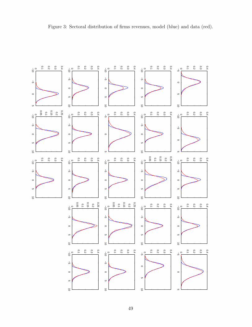
Figure 3: Sectoral distribution of firms revenues, model (blue) and data (red).
−5
05
100
0.1
0.2
0.3
0.4
−10
−5
05
0
0.1
0.2
0.3
0.4
−10
−5
05
100
0.1
0.2
0.3
0.4
−10
−5
05
100
0.1
0.2
0.3
0.4
−5
05
0
0.1
0.2
0.3
0.4
−10
−5
05
100
0.1
0.2
0.3
0.4
−10
−5
05
100
0.1
0.2
0.3
0.4
−10
−5
05
100
0.05
0.1
0.15
0.2
0.25
−10
−5
05
100
0.1
0.2
0.3
0.4
−5
05
100
0.1
0.2
0.3
0.4
−10
−5
05
100
0.1
0.2
0.3
0.4
−5
05
0
0.1
0.2
0.3
0.4
−10
−5
05
100
0.1
0.2
0.3
0.4
−10
−5
05
100
0.05
0.1
0.15
0.2
0.25
−10
−5
05
100
0.1
0.2
0.3
0.4
−10
−5
05
100
0.1
0.2
0.3
0.4
−10
−5
05
100
0.1
0.2
0.3
0.4
−10
−5
05
100
0.1
0.2
0.3
0.4
−10
−5
05
100
0.05
0.1
0.15
0.2
0.25
−10
−5
05
100
0.1
0.2
0.3
0.4
−10
−5
05
0
0.1
0.2
0.3
0.4
−10
−5
05
100
0.05
0.1
0.15
0.2
0.25
−10
−5
05
100
0.1
0.2
0.3
0.4
49

Figure 4: Employment share by decile of city size, model (blue) and data (red).
02
46
810
0
0.05
0.1
0.15
0.2
0.25
02
46
810
0
0.05
0.1
0.15
0.2
0.25
02
46
810
0.02
0.04
0.06
0.08
0.1
0.12
0.14
0.16
0.18
02
46
810
0
0.05
0.1
0.15
0.2
0.25
0.3
0.35
02
46
810
0
0.05
0.1
0.15
0.2
0.25
0.3
0.35
02
46
810
0
0.05
0.1
0.15
0.2
02
46
810
0
0.05
0.1
0.15
0.2
0.25
0.3
0.35
02
46
810
0
0.05
0.1
0.15
0.2
02
46
810
0
0.05
0.1
0.15
0.2
02
46
810
0
0.05
0.1
0.15
0.2
0.25
02
46
810
0
0.05
0.1
0.15
0.2
0.25
0.3
0.35
0.4
02
46
810
0.02
0.04
0.06
0.08
0.1
0.12
0.14
0.16
02
46
810
0.04
0.06
0.08
0.1
0.12
0.14
0.16
02
46
810
0
0.05
0.1
0.15
0.2
0.25
0.3
0.35
02
46
810
0.04
0.06
0.08
0.1
0.12
0.14
0.16
02
46
810
0
0.05
0.1
0.15
0.2
0.25
02
46
810
0.02
0.04
0.06
0.08
0.1
0.12
0.14
0.16
02
46
810
0
0.05
0.1
0.15
0.2
0.25
0.3
0.35
02
46
810
0
0.05
0.1
0.15
0.2
0.25
0.3
0.35
0.4
02
46
810
0.02
0.04
0.06
0.08
0.1
0.12
0.14
0.16
0.18
02
46
810
0.02
0.04
0.06
0.08
0.1
0.12
0.14
0.16
02
46
810
0
0.1
0.2
0.3
0.4
0.5
0.6
0.7
02
46
810
0
0.1
0.2
0.3
0.4
0.5
50

Figure 5: Dilation in firm-size distribution in revenues, large cities vs small cities.
−0.4 −0.2 0 0.2 0.4 0.6 0.8 1−0.4
−0.2
0
0.2
0.4
0.6
0.8
1
Note: For each sector j, dj = log( q75
q25) large− log( q75
q25) small, where ’large’ (resp. ’small’) indexes the set of firms
that locate above (resp. below) the median threshold of city size. q(p) indicates the pth quantile of revenue
distribution. The graph plots this dilation measure dj from the estimated model against dj in the data.
Figure 6: City size distribution, model and data.
8 9 10 11 12 13 14 15 16−10
−8
−6
−4
−2
0
2
4
model: slope= 1.01data: slope= 0.94
All cities
9 10 11 12 13 14 15 16−10
−8
−6
−4
−2
0
2
4
model: slope= 1.07data: slope= 1.02
Right tail
51

Figure 7: Elasticity of productivity with respect to city size: decompositions.
7 8 9 10 11 12 13 14 15 161
1.05
1.1
1.15
1.2
1.25
1.3
1.35
1.4
1.45
Log City Size
Log
Pro
duct
ivity
of F
irms
Firms sort according to their raw efficiencyFirms do not sort according to their raw efficiency
A. Productivity and city size,with and without firm sorting
7 8 9 10 11 12 13 14 15 160
0.2
0.4
0.6
0.8
1
1.2
1.4
1.6
Log City Size
Log
Pro
duct
ivity
of F
irms
Observed log productivityContribution of idiosyncratic shocks (after selection)Contribution of the systematic component
B. Productivity and city size,systematic and idiosyncratic components
7 8 9 10 11 12 13 14 15 160.8
1
1.2
1.4
1.6
1.8
2
Log City Size
Log
Pro
duct
ivity
of F
irms
(Sys
tem
atic
Com
pone
nt)
Firm at 25th percentile of the efficiency distributionFirm at 50th percentile of the efficiency distributionFirm at 75th percentile of the efficiency distribution
C. Systematic productivity and city size,for three levels of firm efficiency
Note: these plots represent averages across sectors. Lines are smoothed for readability. The simulated data have avariance around this line as there is not a unique productivity level for each city-size-sector pair.
52

Figure 8: Aggregate impact of local subsidies, as a function of the cost of the policy.
0 0.5 1 1.5−3.5
−3
−2.5
−2
−1.5
−1
−0.5
0
0.5
Gross Cost of Policy (% GDP)
%
TFP growth (%)Utility growth ( %)
A. TFP and welfare impact,relative to the reference equilibrium
0 0.5 1 1.50
0.2
0.4
0.6
0.8
1
1.2
1.4
1.6
Gross Cost of Policy (% GDP)
%
Change in Gini coefficient for real wage inequality (%)Change in Gini coefficient for city production inequality ( %)
B. Change in the Gini coefficients for real wageinequality and city production inequality
Note: Firms profits are subsidized when they locate in the smallest cities of the reference equilibrium. Thetargeted area represents 2.3% of the population. The policy is financed by a lump-sum tax on firms.
Figure 9: TFP and indirect welfare effects of increasing housing-supply elasticity.
0.90 1.25 1.75 2.45 3.25−5
−4
−3
−2
−1
0
1
2
3
4
Housing−supply elasticity
%
TFP growth (%, relative to median housing supply elasticity)Utility growth ( %, relative to median housing supply elasticity)
The horizontal axis measures housing supply elasticity in the economy dlogHdlogpH
. Saiz (2010) reports that medianelasticity of housing supply is 1.75, the 25th percentile is at 2.45 and the 75th percentile at 1.25.
53

Appendix
A Housing market
Housing supply (equation (2)) and demand (equation (4)) equate so that pH(L) = (1 − η)b w(L)Lb. This yields
the following labor use and profits in the housing sector:
`H(L) = (1− b)(1− η)L, and (30)
πH(L) = b(1− η)Lw(L). (31)
The housing supply elasticity is given by d logH(L)d log pH(L) = η 1−b
b .
Anticipating on the policy discussion, note that a decrease in b increases the housing supply elasticity and also
leads to a flatter wage schedule across city sizes, as d logw(L)d logL = b 1−η
η .
B Extensions of the model
B.1 Log supermodular productivity function
I adapt the model of Davis and Dingel (2012) who microfound complementarity between entrepreneur skill and
city size to a setting where entrepreneurs hire workers to produce output. Workers supply one efficiency unit of
labor. They can also spend a share ψ of their time outside of the firm to gather information that will make them
better at producing the firm blueprint z, such as information on efficient processes of production, or on the appeal
of a product design. The return to this activity is z φ f(L) where the return increases in city size through f(L):
information gathering is more productive when there is more local information available. As a result of this process,
the worker’s amount of labor in efficiency units is: g(z, φ, L) = (1−φ)(1+z φ f(L)). The firm chooses the time spent
on productive activity 1− φ by maximizing their profit, given their production function Y = z kα (` g(z, φ, L))1−α.
As the firm profit function is multiplicatively separable in g(z, φ, L), they choose optimally φ to maximize this
term. This yields an optimized g∗(z, L) = 1f(L)z (f(L)z + 1 − α)(1 + f(L)z)1−α at the optimal φ∗, which can be
shown after some algebra to be log-supermodular in z and L as long as f(L) increases with L (∂2log g∗(z,L)∂z∂L > 0).
B.2 Model with imperfect sorting
Let p(z, Li; j) the probability that a firm of type z in sector j chooses city size Li against other cities Lk for
k = 1, ..., n . As the idiosyncratic shocks to productivity follows a type I extreme value distribution,
p(z, L; j) =π(z, Li, j)n∑k=1
π(z, Lk, j).
It is readily seen that p inherits the log-supermodularity of π in (z, L, j) (abusing notations, j standing for sj or
αj). Therefore the probability distribution of establishments in a high j vs a low j sector follows the monotone
likelihood ratio property. First order stochastic dominance follows.
54

C Proofs
C.1 Lemma 2
Proof Consider a given city of size L developed by city developer i. Let
Nj(L, i) =
∫z
`j(z, L)A(z, L, i)MjdGj(z)
denote the number of workers working in sector j in this specific city i. Equation (8) shows that, for a given city
size and a given sector, labor hired by local firms is proportionate to the ratio of firms profit to the local wage. The
total local profits of firms in sector j is therefore proportional to the sectoral wage bill w(L)Nj . The city developers
problem (11) then simplifies to
maxL,Tj(L)j∈1,...,S
ΠL = b (1− η)w(L)L−S∑j=1
Tj(L)w(L)Nj
(1− αj)(σj − 1)(32)
Free entry pushes the profit of city developers to zero in equilibrium, which drives Tj(L) to T ∗j . The problem is akin
to a Bertrand game. Consider a given city size L. First, any deviation from T ∗j downwards leads a city developer to
loose all firms from the corresponding sector, as new city developers could offer T ∗j for sector j and 0 for all other
sectors, attract all firms for sector j for whom this subsidy is more attractive, and make exactly zero profit. A city
L that attracts only firms from sector j attracts Nj = L − `H(L) = L(1 − (1 − η)(1 − b)
)workers from sector j,
where `H(L) is the labor force hired in the construction sector and the second equality stems from equation (10). It
is readily seen from this expression that the subsidy T ∗j for sector j and 0 for all other sectors leads to zero profits.
Second, any deviation from T ∗j upwards in any sector j leads to negative profits. To see this, consider all cities of
size L, and take the one that offers the highest subsidy city to firms in sector j. Call this city i, and assume that
T ij > T ∗j . From the first step of the proof, we know that in any given city, for all sectors k, either Tk ≥ T ∗k and
Nk ≥ 0 or Tk < T ∗k and Nk = 0. City developer profits in city i are therefore :
Πi = b (1− η)w(L)L−S∑k=1
T ikw(L)N i
k
(1− αk)(σk − 1)
< b (1− η)w(L)L−S∑k=1
T ∗kw(L)N i
k
(1− αk)(σk − 1)
< b (1− η)w(L)L− b(1− η)
1− (1− η)(1− b)w(L)(
S∑j=1
Nk) < 0
where the last inequality comes from∑Sj=1Nk = L− `H(L) and (10).
C.2 Lemma 3
Proof Let Lo denote the suboptimal city size where firms of type (z, j) are located. They get profit π∗j (z, Lo).
Denote ∆ =π∗j (zj ,L
∗(z))
π∗j (z,Lo) − 1 > 0. A city developer can open a city of size L∗(z) by offering a subsidy Tj =
1+ ∆2
1+∆ (1 + T ∗j ) − 1, which will attract firms as they make a higher profit than at Lo, and allows the city developer
to make positive profits. City size distribution adjusts in equilibrium to determine the number of such cities.
55

C.3 Lemma 4
Proof Fix s. Since π(z, L, s) is strictly LSM in (z, L), if follows that for all z1 > z2 and L1 > L2,π(z1,L1,s)π(z1,L2,s)
>π(z2,L1,s)π(z2,L2,s)
. So if z2 has higher profits in L1 than in L2, so does z1. Necessarily, L∗(z1) ≥ L∗(z2).
Moreover, under the technical assumptions made here, L∗j (z) is a strictly increasing function. Since the set of z is
convex, and ψ(z, L, s) is such that the profit maximization problem is concave for all firms, the optimal set of city
sizes is itself convex. It follow that L∗j (z) is invertible. It is locally differentiable (using in addition that ψ(z, L, s)
is differentiable), as the implicit function theorem applies anddL∗j (z)
dz = −∂(ψ2Lψ
)
∂z (z,L∗j (z),s)
∂(ψ2Lψ
)
∂L (z,L∗j (z),s)
.
C.4 Lemma 5
The proof is in the main text.
C.5 City size distribution
I establish here the following characterization of the city-size distribution.
Characterization 10 If the firm size distribution in revenues follow Zipf ’s law, a sufficient condition for the city
size distribution to follow Zipf’s law is that revenues have constant elasticity with respect to city size in equilibrium,
under realistic parameter values.
When the productivity function is log(ψj(z, L, sj)) = aj logL+log(z)(1+log LLo
)sj , equilibrium firm-level revenues
have constant elasticity with respect to city size in equilibrium.
Proof There is a bijection between z and firm level observable at equilibrium r∗, `∗, L∗. By an abuse of nota-
tion, this functional relationship will be denoted z(r), z(L), `(z). All of these relationship pertain to the sorting
equilibrium, but I omit the star to keep the notations light.
Step 1: Write gj(r) the distribution of revenues in sector j. The firm-size distribution in revenues is readily
computed through a change of variable, starting from the raw efficiency distribution:
gj(r) = fj(z(r))dz
dr(r) (33)
Step 2: Assume that in all sectors - or at least for the ones that will locate in the largest cities in equilibrium -,
firm-size distribution in revenues is well approximated by a Pareto distribution with Pareto shape ζj , close to 1.
Write gj(r) the distribution of revenues in sector j:
∃rj,o : ∀ r > rj,o, gj(r) ∝ r−ζj−1 (34)
Step 3: The city size distribution fL(.) as defined by equation 20 can be written as:
fL(L) =
S∑j=1
Mj f j(L)
where f j(L) =`j(z
∗j (L)) fj(z
∗j (L))
dz∗j (L)
dL
L . Then,
56

f j(L) ∝ gj(r∗(L))
dr∗jdL
rj(L)
Lbη
1−η+1
∝ rJ(L)−ζj+1
Lbη
1−η+2
The first line uses (33), `j ∝ rj(L)w(L) and w(L) ∝ Lb
η1−η . The second line uses the assumption that r∗ has constant
elasticity with respect to L at the sorting equilibrium, and (34). As ζ ∼ 1,
f j(L) ∝ 1
Lbη
1−η+2and fL(L) ∝ 1
Lbη
1−η+2.
Finally, b η1−η << 1, as it measures the elasticity of wages with city size, on the order of magnitude of 5%. The
tail of the city size distribution is well approximated by a Pareto of shape close to 1. City size distribution follows
Zipf’s law.
C.6 Proposition 6
Proof Fix j. For productivity, the results comes from the facts that (1) L∗j (z) is non decreasing in z and (2) that
ψ(z, L, sj) is increasing in L. Revenues are proportional to profits (rj ∗ (z) =σj
1+T∗jπ∗j (z)). The proof for profits is
as follows. ψ(zH , LL, sj) > ψ(zL, LL, sj) as ψ is increasing in z, which leads to π(zH , LL) > π(zL, LL), as firms
face the same wage in the same city. Finally, π(zH , LH , sj) ≥ π(zH , LL, sj) as LH is the profit maximizing choice
for zH . Therefore, π(zH , LH , sj) > π(zL, LL, sj).
In addition, εl = εr − (1− α) 1−ηη .
Proof For a given city size L and a given sector j, r∗j (L) =∑z in L r
∗j (z) ∝
∑z in L w(L)`∗j (z) ∝ w(L) ¯∗
j (L),
where their proportion is constant across city sizes. Therefored log ¯∗
j (L)
d log L =d log r∗j (L)
d log L − εw, where the elasticity of
wages with respect to city sizes is εw = b η1−η
C.7 Proposition 7
Proof The proof here covers both the case of the main assumptions of the model (continuity and convexity of
the support of z and L), and the case where the set of city sizes is exogenously given, and in particular discrete.
Let Z : L x A x E → Z be the correspondence that assigns to any L ∈ L and α ∈ A a set of z that chooses L
at equilibrium. (It is a function under the assumptions made in the main text (see proof of Lemma 4).) Define
z(L,α, s) = maxzz ∈ Z(L,α, s) as the maximum efficiency level of a firm that chooses city size L in a sector
characterized by the parameters (α, s). I will use the following lemmas:
Lemma 11 log π is supermodular with respect to the triple (z, L, α)
It is readily seen that: ∂2log π(z,L,α,s)∂z∂L > 0, ∂
2log π(z,L,α,s)∂z∂α = 0 and ∂2log π(z,L,α,s)
∂L∂α = (1−η)γL > 0. This result does not
rely on an assumption on the convexity of L. Checking the cross partials are sufficient to prove the supermodularity
even if L is taken from a discrete set, as π can be extended straightforwardly to a convex domain, the convex hull
of L.
Lemma 12 z(L,α, s) is non decreasing in α, s.
57

The lemma is a direct consequence of the supermodularity of log π with respect to the quadruple (z, L, α, s).
Using a classical theorem in monotone comparative statics, if log π(z, L, α, s) is supermodular in (z, L, α, s), and
L∗(z, α, s) = maxL log π(z, L, α, s) then (zH , αH , sH) ≥ (zL, αL, sL)⇒ L∗(zH , αH , sH) ≥ L∗(zL, αL, sL). Note that
everywhere, the ≥ sign denotes the lattice order on R3 (all elements are greater or equal than).
Coming back to the proof of the main proposition, we can now write:
F (L;α, s) = P (firm from sector(α, s) is in a city of size smaller that L)
= F (z(L,α, s))
where F (.) the the raw efficiency distribution of the firms in the industry. Let αH > αL.
For any z ∈ Z, the previous lemma ensures that L∗(z, αH , s) ≥ L∗(z, αL, s). In particular, fix a given L and s and
write using shorter notation: zαL = z(L,αL, s). Then L∗(zαL , αH , s) ≥ L∗(zαL , αL, s) = L. Because L∗(z, αH , s) is
increasing in z, it follows that:
z ∈ Z(L,αH , s)⇒ z ≤ zαL
and therefore zαH ≤ zαL or using the long notation: z(L,αH , s) ≤ z(L,αL, s)It follows that F (z(L,αH)) ≤ F (z(L,αL)) and that F (L;α, s) is decreasing in α. This completes the proof of the
first order stochastic dominance of the geographic distribution of a high α sector vs that of a lower α.
The proof is exactly the same for the comparative static in s, we just have to verify that π(z, L, s) is log supermodular
in (z, L, s). Since π(z, L, sj) = κ
(ψ(z,L,sj)w(L)1−α
)σ−1Rj
P 1−σj
and w(L) doesn’t depend on s, π(z, L, s) directly inherits the
log supermodularity of ψ(z, L, s) in its parameters.
C.8 Proposition 8
Proof The proof here covers both the case of the main assumptions of the model (continuity and convexity of
the support of z and L), and the case where the set of city sizes is exogenously given, and in particular discrete.
Within sectors, the revenue function r∗j (z) at the sorting equilibrium is an increasing function for any j. Let
p1 < p2 ∈ (0, 1). Under the assumption, maintained throughout the comparative static exercise, that sectors draw
z from the same distribution, there ∃ z1 < z2 such that Qj1(p1) = r∗j1(z1) and Qj2(p1) = r∗j2(z1) (same thing for
z2 and p2), ie. the quantiles of the r∗j1 and r∗j2 distributions correspond to the same quantile of the z distribution.
This yieldsQj1 (p2)
Qj1 (p1) =r∗j1(z2)
r∗j1(z1) , andQj2 (p2)
Qj2 (p1) =r∗j2(z2)
r∗j2(z1) .
Finally, it is a classic result in monotone comparative statics (Topkis (1998)) that if π(z, L, α) is log-supermodular
in (z, L, α), then π∗(z, α) = maxL π(z, L, α) is log supermodular in (z, α), orπ∗j2(z2)
π∗j2(z1) ≥π∗j1(z2)
π∗j1(z1) . Revenues are
proportional to profits within sectors, which completes the proof. The same proof applies for s.
C.9 Corollary 9
Proof Let pj ∈ (0, 1) be a threshold above which the distribution is well approximated by a Pareto distribution
in sector j, and rj the corresponding quantile of the distribution. The distribution of r conditional on being larger
than rj is:
∀r > rj , Hj(r | r ≥ rj) ≈ 1− (r
rj)−ζj ,
58
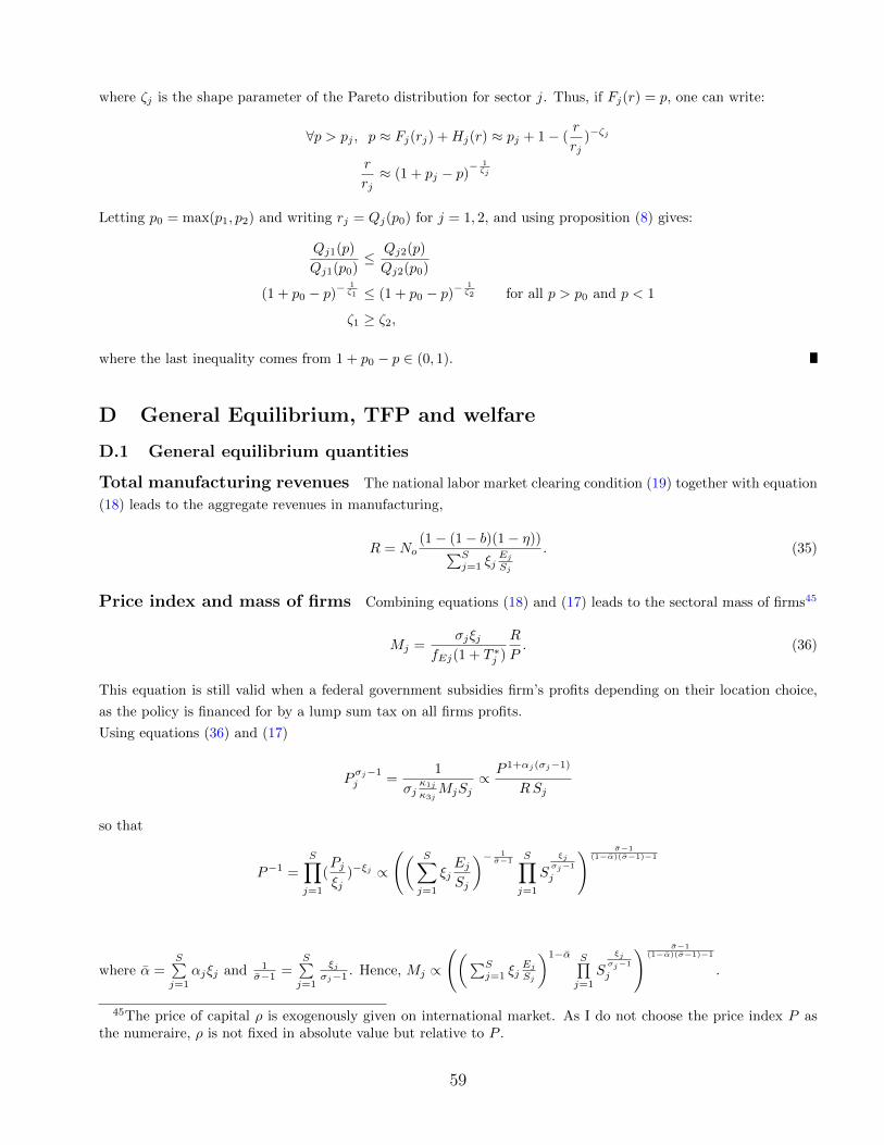
where ζj is the shape parameter of the Pareto distribution for sector j. Thus, if Fj(r) = p, one can write:
∀p > pj , p ≈ Fj(rj) +Hj(r) ≈ pj + 1− (r
rj)−ζj
r
rj≈ (1 + pj − p)
− 1ζj
Letting p0 = max(p1, p2) and writing rj = Qj(p0) for j = 1, 2, and using proposition (8) gives:
Qj1(p)
Qj1(p0)≤ Qj2(p)
Qj2(p0)
(1 + p0 − p)−1ζ1 ≤ (1 + p0 − p)−
1ζ2 for all p > p0 and p < 1
ζ1 ≥ ζ2,
where the last inequality comes from 1 + p0 − p ∈ (0, 1).
D General Equilibrium, TFP and welfare
D.1 General equilibrium quantities
Total manufacturing revenues The national labor market clearing condition (19) together with equation
(18) leads to the aggregate revenues in manufacturing,
R = No(1− (1− b)(1− η))∑S
j=1 ξjEjSj
. (35)
Price index and mass of firms Combining equations (18) and (17) leads to the sectoral mass of firms45
Mj =σjξj
fEj(1 + T ∗j )
R
P. (36)
This equation is still valid when a federal government subsidies firm’s profits depending on their location choice,
as the policy is financed for by a lump sum tax on all firms profits.
Using equations (36) and (17)
Pσj−1j =
1
σjκ1j
κ3jMjSj
∝ P 1+αj(σj−1)
RSj
so that
P−1 =
S∏j=1
(Pjξj
)−ξj ∝
(( S∑j=1
ξjEjSj
)− 1σ−1
S∏j=1
S
ξjσj−1
j
) σ−1(1−α)(σ−1)−1
where α =S∑j=1
αjξj and 1σ−1 =
S∑j=1
ξjσj−1 . Hence, Mj ∝
((∑Sj=1 ξj
EjSj
)1−α S∏j=1
S
ξjσj−1
j
) σ−1(1−α)(σ−1)−1
.
45The price of capital ρ is exogenously given on international market. As I do not choose the price index P asthe numeraire, ρ is not fixed in absolute value but relative to P .
59

D.2 TFP and welfare
TFP Let Yj , Nj and Kj denote the sectoral output, employment and capital. Sectoral productivity TFPj ≡Yj
Kαjj N
1−αjj
can be expressed as follows.
Yj = M1
σj−1
j
(∫ (ψ(u, L∗j (u), sj) k
∗j (u)αj `∗j (u)1−αj
)σj−1
σj dFj(u)
) σjσj−1
= Kαjj N
1−αjj M
1σj−1
j
(∫ (ψ(u, L∗j (u), sj) o
kj (u)αj o`j(u)1−αj
)σj−1
σj dFj(u)
) σjσj−1
, (37)
where
o`j(z) =`∗j (z)
Nj=
ψ(z,L∗j (z),sj)σj−1
w(L∗j (z))(1−αj)(σj−1)+1∫ (ψ(u,L∗j (u),sj)
σj−1
w(L∗j (u))(1−αj)(σj−1)+1
)dFj(u)
, and
o`k(z) =k∗j (z)
Kj=
ψ(z,L∗j (z),sj)σj−1
w(L∗j (z))(1−αj)(σj−1)∫ (ψ(u,L∗j (u),sj)
σj−1
w(L∗j (u))(1−αj)(σj−1)
)dFj(u)
.
(38)
After some algebra, this leads to
TFPj = M1
σj−1
j
(∫ψ(u,L∗j (u),sj)
σj−1
w(L∗j (u))(1−αj)(σj−1)+1 dFj(u)
) σjσj−1−αj
(∫ψ(u,L∗j (u),sj)
σj−1
w(L∗j (u))(1−αj)(σj−1)+1 dFj(u)
)1−αj
TFPj = M1
σj−1
j
Sjσjσj−1−αj
Ej1−αj , (39)
where Sj and Ej are defined in the main text. Sectoral TFP only depends on the matching function L∗j (z) and the
wage schedule elasticity with respect to city size. To see this, consider the wage schedule defined by equation 6.
The wage level w(1− η)b1−ηη does not enter expressions (38). The absolute wage level cancels out in the expression
of the ratios o`j(z) and okj (z). It follows that the absolute wage level does not impact equations (37) or (39).
Decomposing Welfare
TFPj = M1
σj−1
j (SjEj
)1−αjS1
σj−1
j
Given equation (36) and the expression for the price index,
P−1j = TFPj(
EjSj
1−αj)
1
Pαj
P−1 ∝( S∏j=1
TFPξjj
(EjSj
)ξj(1−αj)) 11−α
60