Embed Size (px)
Citation preview

Firm Productivity, Worker Ability, and
Returns to Education
Garth Frazer
University of Toronto
Abstract This paper takes a different approach to wage equation estimation–that of the firm. In the
human-capital/competitive-market model, the coefficients in the wage equation estimate the skill
production function. The paper demonstrates (and proves) that this skill production function is
also the labour term in a firm production function, providing a new method for estimating, for
example, the schooling coefficient in a Mincer equation. In addition, inclusion of this skill
production function in the labour term of a firm production function opens up a new methodology
for acquiring a measure of unobserved worker ability, which can then be used as a direct control for
ability in a wage regression. While the wage equation human capital coefficients should be
identical to the production function human capital coefficients, the methodology allows for testing
to determine whether various characteristics such as schooling are remunerated according to their
productivity. Since a productivity-based definition of worker ability is included in the wage
estimation, this not only avoids the traditional ability bias, but also other forms of endogeneity
that occur after the schooling decision. The methodology is tested in the context of Ghana, a
setting where the accurate measurement of returns to education is particularly important. Using
this method, the internal rate of return to education is estimated at roughly 7%, after correcting
for an average ability bias of approximately 3%.
Keywords: returns to education, productivity, linked employer-employee datasets, Africa,
structural estimation of production functions JEL Classification Numbers: J24, J30, D24, O12
1 Introduction
Estimating wage equations is at the heart of labor economics. Determining the productive
contribution of various characteristics to a person’s productivity, and therefore one’s wage
is one of the central questions in the field. For example, accurately determining the causal
impact of education on earnings is a central question that requires estimation of a wage
equation. Such an equation is of the form:
(1) w = f(X;β) + ε
where w is the natural logarithm of the wage (the specification used for the dependent
variable in virtually all studies), and f is either a parametric or semi-parametric function
of observable characteristics, denoted by the vector X, and the associated parameter vector
β. Since schooling is virtually always one of the X variables, one of the central questions
that has been estimated in such regressions has been the returns to schooling. Typically,
the theoretical model that is underlying the wage equation above is some form of human
capital model (following Becker (1964), Ben-Porath (1967) and Mincer (1974)), where the
schooling is an investment in human capital made early in one’s life, resulting in an increase in
productivity and therefore wages later in life from the increased human capital. In addition,
in the Mincer (1974) model, the coefficient on schooling also represents an internal rate of
return on the schooling investment, under assumptions that are shown to be fairly restrictive
by Heckman, Lochner, and Todd (2006). In addition, Wolpin (2003) highlights the fact that
the interpretation of the coefficients (including schooling) in such a wage equation depend
on the specific model assumed to be operable, and that the interpretation of the schooling
coefficient is different, for example, in the context of a search model.
Still, the vast majority of explorations of wages with the above equation have been
working from a model of human capital.1 In the human capital model, the observable
characteristics, X, increase an individual’s productive skill. As noted in Griliches (1977),1In addition to the search model interpretations of the above wage equation, signalling models also allow
1
for example, in the case of a competitive market for this skill, the f function can be broken
into the a person’s skill, and the remuneration for that skill:
(2) w = pS + g(X;β) + ε
where pS is the natural logarithm of the market-determined price for skill, and the g
function represents an individual’s skill level. With such an interpretation, the intercept in
a wage regression captures the skill price in the economy.2
As mentioned, a central concern in such an equation relates to its estimation using least-
squares regression. In such a context, we would expect that the error term, ε, which contains
unobservable characteristics and factors, such as a person’s ability, would certainly be cor-
related with the observable characteristics, such as schooling, resulting in biased parameter
estimates. Typically, most labor economists expect that individuals of higher ability will
also obtain higher schooling, resulting in an upward-biased estimate of the return to school-
ing, but as noticed from the early writers (Griliches (1977)), that bias could be downward
as well under certain conditions. Different strands of the literature have taken different
approaches to deal with this problem. Card (1999) summarizes a couple of strands of this
literature including the use of twins as a natural experiment in different levels of schooling,
as well as the use of instrumental variables such as distance to college or school, parental
education, quarter of birth, or other natural or policy-based experiments to instrument for
the level of schooling. In contrast, the structural labor literature (e.g. Belzil and Hansen,
2002; Keane and Wolpin, 1997) has estimated the unobservables in the context of a dynamic
model.
The goal of this paper is to develop a method for estimating the β parameters in the
above wage equation, but the method employed is entirely different from previous work.
for different interpretation of the coefficients. In signalling models, schooling does not lead to productiveincreases in skill, but merely signals to employers higher ability.
2Note that this can be generalized to a Roy (1951) model where there are different returns to observablecharacteristics in separate sectors/occupations, and therefore different wage equations (and therefore differentg functions) in different sectors/occupations, with one such equation for each sector.
2
Here, I take the perspective of the firm. In a human capital model, the g functional form
represents the productive return to observable characteristics, that is the skill production
function, and so the starting point is to recognize (and then prove) that the g function can
also be found in a production function of a firm. Once this is accomplished, the techniques
in the literature on production function estimation that allow for consistent estimation of
production function parameters become available. This is advantageous because in the
competitive-market/human-capital model, these coefficients should be the coefficients on
productive coefficients in the wage equation (to be proved shortly). Moreover, if we have an
independent method of estimating the wage equation parameters consistently (using either
structural or non-structural approaches), we can in fact test the human-capital/competitive-
market model for wage determination, by comparing the production function parameters to
the wage equation parameters. In addition, estimating the production function provides
us a new method to directly obtain measures of unobservable worker ability (similar to the
structural labor literature, but using information from the firm perspective). With the
inclusion of these unobservable productive attributes, we can consistently estimate the wage
equation highlighted above.
To be specific, consider the coefficient on schooling in skill production function (g) above.
The Mincer specification, which has been found to fit the data reasonably well in a wide
variety of different countries and datasets, specifies the g function with a linear term in
schooling and a quadratic function in experience. While this is based on a particular
(restrictive) theoretical model in Mincer (1958) and Mincer (1974), this functional form has
been widely replicated because of its applicability, although improvements have certainly
been made in some contexts and with some datasets.3 The major issue in the estimation
of the schooling coefficient is the issue of ability bias—that the schooling variable will be
3Heckman, Lochner, and Todd (2006) demonstrate that using higher order terms in schooling and expe-rience, as well as their interactions provides a better fit to recent U.S. data. They also raise a number ofother issues in their paper which will be addressed in the current paper.
3

correlated with unobserved individual ability, which is part of the ε term in the above wage
equation so that estimation by least squares will result in biased parameter estimates.
Inclusion of an appropriate measure of worker ability in the wage regression would address
the ability bias problem. While there has been some debate about whether, for example, IQ
is an adequate measure of worker ability, the definition of ability that matters for estimating
a wage equation is the part that contributes to productive skill, because that is the part of
human ability that, if observable, should be included in the g function in (2) above. The
advantage of approaching the issue of estimating the g function from the production function
side is that the productive unobserved skill of the workers is the exact definition of ability
that turns out to be estimable from a production function. This measure can be used in a
wage equation to control directly for ability, and avoid problems of ability bias.
In fact, the measure of worker ability that is included in this regression is able to address
additional issues. Worker ability is typically assumed to be static, and so the ability bias
issue is typically framed in a static context. Here, worker ability can change over time.
This relates to the Rosenzweig and Wolpin (2000) critique of the twins’ literature in the case
where the error term contains endogenous post-schooling choices, or when schooling impacts
on future opportunity sets and choices.4 When the control for unobserved productive ability
is included, this controls for these post-schooling choices, which either end up being revealed
in the form of productive skill, and therefore controlled for directly, or are irrelevant from
the perspective of the g function.
Therefore, in short the goal of the paper is to provide a novel mechanism for estimating
the β parameter vector in the human capital production function, g, above, by approaching
the issue from the perspective of the firm. This is not the first paper to include a school-
ing variable in some form in a production function.5 However, this is the first study to
4A more important limitation of twins’ studies of returns to schooling in the developing country contextis the simple lack, to my knowledge, of any twins’ datasets.
5The inclusion of schooling and experience into a production function is not new to this study, but wasused in Bils and Klenow (2000), and has been used with firm data in Jones (2001), Bigsten et. al. (2000),
4
demonstrate the production function that is consistent with the specification in (1) above,
and therefore the production function that is consistent with, in particular, the widely-used
Mincer specification. Estimating this production function allows for a different method of
consistently estimating the g function above. In addition, it allows us to test whether the
human-capital/competitive-market model for wage determination holds for some or all of the
X characteristics in the g function. This allows us to test questions such as the following. Is
the productive return to schooling greater than its remuneration? What about experience,
or other worker characteristics, that might reflect some form of discrimination?6 Clearly,
there are a wide variety of questions that can be explored by comparing the productive and
remunerative return to different worker characteristics.
The assumptions required to prove that the g function above occurs in firm produc-
tion functions are simply those of the human-capital model with a competitive market in
skill. Therefore, provided that the parameters of the production function are estimated con-
sistently, we should obtain consistent parameters of the parameters of the g function. To
obtain consistent estimates of the production function parameters, we follow the state-of-the-
art in the industrial organization literature on production function estimation, as identified
in a survey article by Griliches and Mairesse (1998).7 This literature has a widely-used
set of common assumptions that form the basis of the production function estimation. In
essence then, what the approach in this paper does is replace the non-structural or struc-
tural assumptions of the wage equation estimation literature in labor economics with the
commonly-used assumptions in the industrial organization literature on estimating produc-
and Hellerstein, et. al. (1999). The inclusion of ability, and the incorporation of standard wage equationspecification (where log(wage) is the dependent variable) into the production function is new to this study.
6These questions have been studied, with a different set of assumptions, and functional forms in Hellersteinet. al. (1999).
7While Griliches and Mairesse discuss the advantages of using the Olley and Pakes (1996) approach toproduction function estimation, I use the technique of Ackerberg, Caves and Frazer (2006), which uses thesame assumptions as Olley and Pakes approach, but is immune to a collinearity critique that Ackerberg,Caves and Frazer identify as applying to both the Olley and Pakes method, and the Levinsohn and Petrin(2003) methods of production function estimation.
5

tion functions. Since these assumptions are markedly different from those employed in
either the structural or non-structural labor literature, they provide an independent method
for estimating the g function coefficients. The primary limitation in this approach is that
it requires the estimation of a production function, and therefore requires linked employer-
employee data, including the data required for production function estimation on the firm
side, as well as data on (at least a sub-sample of) the workers at these firms on the employee
side.8
The context where I explore these questions is the context of Ghana. The reason for this
setting is threefold. First, linked employer-employee data is available for Ghana. Second,
knowledge of the β parameters, and in particular the returns to schooling in the Ghanaian
context is a crucial policy question in a context where resources are comparatively limited,
and therefore competition for government budget dollars is exceptionally intense. Third,
in developing country contexts, where it is very difficult to effectively separate poor from
non-poor in targeted poverty programs, education is one of the most important anti-poverty
programs.9 In this context, even knowledge of the private returns to education (which
provide a lower bound to the social returns) is important from a development, anti-poverty
perspective. Furthermore, understanding the importance of education is particularly pointed
in Africa, which has experienced lower growth and lower levels of education than all other
regions over the past thirty years, and yet the growth of the stock of education has been
more rapid in Africa than elsewhere (Nehru et. al., 1995). Despite this fact, there has been
comparatively little "best practice" research done for African countries (Appleton, et. al.,
1996; Behrman, 1996). Therefore, in addition to demonstrating the general technique of
estimating the g function above using firm-level information, this paper also uses the above
8See Abowd and Kramarz (1999) for a survey of the linked employer-employee literature.9Some studies which have examined the returns to schooling in the context of developing countries include:
Behrman and Deolalikar (1991) - Indonesia ; Behrman, et. al., (1999) - India; Duflo (2001) - Indonesia;Godana (1997) - Zimbabwe; Li and Zhang (1998) - China; Mwabu and Schultz (1996) - South Africa,Nielsen and Westergård-Nielsen (2001) - Zambia; Ram and Singh (1988) - Burkina Faso; Siphambe (2000) -Botswana; Smith and Metzger (1998) - Mexico; Lassibille and Tan (2005) - Rwanda.
6

technique to examine the concrete question of ability bias in the measurement of returns to
education in the context of Ghana.10
Although the approach used here is quite different from the structural literature, the
estimated Mincer coefficient is similar. Specifically, the results reveal an upward bias on
the education coefficient, which is the direction of ability bias most often expected by labor
economists. It is found that the returns to schooling vary by schooling level, even using the
standard Mincer specification, but the average results are between 6 and 7%, in each case
roughly 3% below the estimate based on OLS results. The outline of this paper is as follows.
Section 2 outlines the incorporation of the Mincer specification into the production function,
including the issue of ability bias, and the production function specification. Section 3
describes the wage equation estimation. Section 4 describes the data used for estimation,
with the results in Section 5, and a brief conclusion in Section 6.
2 Modeling the Production of the Firm
A frequent specification for production function estimation is the Cobb-Douglas form, which,
written in logarithmic form, using lower-cased variables, is:11
(3) yft = β0 + βllft + βkkft + εft
where y is the value-added, l the labor, and k the capital of firm f in period t. Estimation
of equation (3) by least-squares raises two concerns. The first, the problem of simultaneity
bias, has been understood in the literature at least since Marschak and Andrews (1944),
although satisfying solutions to this problem have only arisen recently (Olley and Pakes,
1996; Levinsohn and Petrin, 2003; Ackerberg, Caves, and Frazer (2006)). The second is the
10Glewwe (1999) estimates a Mincer coefficient on education for Ghana for the period 1998-99 (GhanaLiving Standards Survey (GLSS) - Round 2), the most comparable results to our own. He finds that theOLS measure of the returns to education is 8.5%. Using the GLSS data which is closest to the time periodof the data under investigation here, the GLSS Round 4 data for 1998-99, we find that the OLS estimatehas changed little, and is now 8.8% (author calculation).11Throughout this paper, upper-cased Roman letters will refer to the standard form of variables, and lower
cased letters their natural logarithms.
7

assumption of homogeneous labor, in that the variable l is typically specified as the number
of employees or the number of worker-hours at a firm, or at best split into two types at
the firm level. Considerable effort, therefore, will be given in this paper to improving the
labor term in the production function. First, however, let us briefly examine the problem
of simultaneity, which will also be addressed in this paper.
The simultaneity problem arises because the error term includes firm productivity, which
is seen by the firm manager and will very likely be correlated with this period’s labor input,
which is typically considered to be freely variable. It is typically not assumed to be correlated
with this period’s capital stock, which is generally considered to have been determined last
period.12 If some additional assumptions are made on the correlations between capital, labor
and the error term, the simultaneity bias will result in an upward bias on the labor coefficient,
and possibly a downward bias on the capital coefficient (Levinsohn and Petrin, 2003). The
current standard approach in the production function literature builds on the work of Olley
and Pakes (1996).13 In short, they separate the error term into firm productivity, ωft, which
is seen by the firm manager, and ηft, which is a pure noise residual, including for example,
measurement error in output. The production function then becomes:
(4) yft = β0 + βllft + βkkft + ωft + ηft
In the Olley and Pakes model, the productivity term is derived in the context of a dynamic
model to be a nonparametric function of investment and the firm’s capital stock, at least
when investment is strictly positive. While restricting to observations with non-zero in-
vestment forces Olley and Pakes to lose 8 percent of their observations, in other datasets
(such as the current one) this can force deletion of a much larger fraction of observations,
and frequently the majority of observations in developing country datasets.14 To overcome
12This paper requires a much weaker assumption on the capital stock than this, as outlined in AppendixA3.13See Griliches and Mairesse (1998) for a fuller discussion of the advantages of this approach.14For example, following the Olley-Pakes approach would require deletion of 56 percent of the observations
used in the Ghanaian dataset used in this study.
8
this limitation, Levinsohn and Petrin (2003) modify the Olley and Pakes procedure to use
intermediate inputs, instead of investment, in the estimation of firm productivity. Unfor-
tunately, both of these procedures have come under a methodological critique regarding the
(lack of) identification of the labor coefficient in these estimation procedures (Ackerberg,
Caves, and Frazer, 2006). This study therefore uses the procedure of Ackerberg, Caves, and
Frazer (2006), which builds on both of the Olley/Pakes and Levinsohn/Petrin methodologies,
but is immune to the critique. The current paper also modifies the Ackerberg, Caves, and
Frazer (2006) procedure by including human capital variables in the production function, as
described below and in Appendix A.3.
As mentioned, the other problem of simple estimation of equation (3) is the assumption
of homogeneity of labor. This simplification reflects the limitations of the data which
have typically been available for estimation. Fortunately, with the increasing availability of
linked employer-employee datasets, which provide data on at least a sub-sample of, a firm’s
employees, we can now ask the question of what is a more sensible specification for labor’s
contribution to firm product.
The approach taken is immediately applicable to almost any functional form of a wage
equation where the natural logarithm of the wage is the dependent variable (equation (1)),
which is the specification used in essentially all forms of wage equation estimation. For
clarity, the approach will be delineated for a Mincer specification, and that will be the
benchmark specification used in the estimation. Generalizations to this functional form will
be discussed later. A Mincer (1974) specification for the wage equation, with the addition
of an ability term would be:
(5) wi = λ0 + λSSi + λXXi + λYX2i + λAAi + υi
where S represents years of schooling, A represents ability, and X represents potential
experience (X = G−S− 6), with G representing age. Heckman, Lochner and Todd (2006)
summarize the two models outlined by Mincer (1958, 1974) develops models under which
9
the coefficient λS can also be interpreted as the internal rate of return to an additional year
of schooling investment, calculated at the start of an individual’s life.15 If ability is omitted
from regressions estimating the above equation, the schooling coefficient will be biased, as
noticed at least since Becker (1964). A variety of approaches have been used to address this
problem, and these approaches, and their limitations, are summarized in survey articles by
Card (1999) and Belzil (2007). As Griliches (1977, p. 5) notes, “the simplest way of dealing
with this problem is to find a measure of ‘ability’ and include it in such an equation,” and
such an approach was common in the earlier literature (Griliches and Mason, 1972; Griliches,
1976; Griliches, 1977). However, as Griliches (1977) notes in the same article, the value
of using IQ-measures as ability controls was controversial: “Two polar views are possible.
‘Ability’ is IQ, or something close to it, and the only problem is that our measures of it are
subject to possibly large (test-retest) errors...The alternative view is that ‘ability’, in the
sense of being able to earn higher wages, other things equal, has little to do with IQ.” (p.
7) In the subsequent 25 years, the latter view has held sway, as IQ or other test-related
measures have not often been used to control for ability bias. The current study uses a
direct control for ability, but not one which is obtained from an IQ-type test, but rather one
which is revealed through an individual’s productivity.
The direct control for ability which has at times been used in the developing country con-
text, the Raven Progressive Matrices test, has virtually always been insignificant in log(wage)
regressions of the above form (Boissiere, et. al., 1985; Knight and Sabot, 1990; Alderman,
Berhman, Ross and Sabot, 1996; as well as Glewwe, 1996; Glewwe, 1999 in the context of
Ghana), although Alderman, Berhman, Ross and Sabot (1996) do find it to have a small,
significant impact on wages in Pakistan, without the inclusion of other controls.16 While
15Heckman, Lochner and Todd (2006) abstract from the issue of ability bias, but they calculate the internalrate of return to various levels of schooling, allowing for nonparametric treatments of both the schooling andexperience variables, and accounting for tuition, taxes, uncertainty, and assumptions about agent expectationformation. This paper will address many of the important issues raised by their paper.16Alderman, Behrman, Khan, Ross, and Sabot (1997) look at the impact of ability on cognitive achievement
in reading and mathematics, and find that the Raven’s test scores do have a significant effect on reading and
10

it may be true that ability has no independent effect on a person’s earnings, resulting in
the repeatedly insignificant coefficient, it may also be true that the Raven’s test provides an
inadequate measure of workplace ability. This paper is motivated by the latter possibility.
The total human capital available at the firm can be obtained by summing the human
capital of all of its workers. For the Mincer specification, including ability, an individual’s
skill (the g function of equation (2)) is g(X;β) = eλSSi+λXXi+λAAi+ξi, and so the total human
capital at the firm is:Pι
(eλSSi+λXXi+λAAi+ξi). Label the price of this human capital as pH ,
and recall that pH = eλ0. Then, the total value of the human capital is also the firm’s wage
bill:17
(6)Xι
(eλ0+λSSi+λXXi+λAAi+ξi)
If the firm is optimizing (given that the firm is a price-taker in wages), the productive
contributions of workers’ characteristics should reflect the relative costs of these character-
istics. In order for this to be the case, the labor term in the production function should
have the same form as (6). That the labor term in the production function should have
the same form as the wage bill for a profit-maximizing firm is proved in Appendix A.1.
Therefore, the production function which is consistent with a Mincerian wage equation is
F [P
Ljeλ∗0+λSSj+λXXj+λAAj ,K,Q,M ]. Here, M and Q are two components of firm pro-
ductivity that will be discussed subsequently, and the number of workers of type j with
characteristics (Sj,Xj, Aj) is Lj (so thatP
Lj = L is the total number of workers at the
firm, and Lj = 0 for types that are unused by the firm). Therefore, defining the price of
output as p, the profit function for the firm is:
(7) Π = pF [P
Ljeλ∗0+λSSj+λXXj+λAAj ,K,Q,M ]−PLje
λ0+λSSj+λXXj+λAAj+ξj − rK
mathematics achievement test scores.17In this case, a linear experience term is used. However, note that the analysis can be extended to a
quadratic in experience, and to the inclusion of additional controls, as it is for estimation purposes in thispaper. In that case, the experience-squared term (and other terms) receive the same treatment as theschooling term and the experience term. These other terms are omitted from the exposition for simplicity.
11
The cost of capital is r. The choice variables for the firm are the values for each
of the Lj’s, as well as K, with the first term of the production function labelled equally as
human capital, or the quality of labor, or effective labor.18 While, by Appendix A.1, the
coefficients on an individual’s schooling in the production function must equal that on the
wage equation in the above profit function, so that the parameters of our g function can be
derived from the production function, this restriction will be tested, rather than imposed on
the data. Therefore, the profit function that will be considered is of the form:
(8) Π = pF [P
Ljeβ1+βSSj+βXXj+βAAj ,K,Q,M ]−PLje
λ0+λSSj+λXXj+λAAj+ξj − rK
After estimating the production function, and the wage equation separately, the equalities
βS = λS and βX = λX will be tested. Following the literature standard, the technology for
F will be Cobb-Douglas, and therefore the production function to be estimated is:
(9) Y = eβ0(P
Ljeβ1+βSSj+βXXj+βAAj)βHKβK (eMeQ)βωeε
In equation (9), for the summation to calculate labor quality, the only types that matter
are those chosen in positive quantity (Lj > 0), so that this term can be re-indexed by the
i = 1, ..., L workers chosen at a firm to get:
(10) Y = eβ0(LPi=1
eβ1+βSSi+βXXi+βAAi)βHKβK(eMeQ)βωeε
The subscripts for firm f and time t remain omitted for this discussion of functional form,
but will be introduced subsequently. If we use the logarithmic Cobb-Douglas form, by taking
logarithms of both sides of the equation, and representing each variable’s natural logarithm
using its lower-cased letter, then:
(11) y = β0 + log(LPi=1
eβ1+βSSi+βXXi+βAAi)βH + βKk + βω(M +Q) + ε
18To be precise, it is assumed that the labor force is dense enough that the firm is able to choose the valueof Lj for each of the possible three-tuples (Sj ,Xj , Aj) in the space of the domain. For the purposes of theempirical investigation, Sj and Xj will be measured in integral values from 0 to say 30 and 90, respectively.For consistency of exposition here, think of Aj as taking on values between 0 and 100. The actual domaindefinitions are inconsequential for the analysis that follows, but are given for completeness. All of thearguments that follow carry through to the continuous case.
12

Now, if we observed measures for each of the variables in the estimation procedure then
equation (11) could be estimated using a non-linear method. Such estimation would require
knowledge of the distribution of workers at the firm (or at least a sample estimate of the
distribution), and their schooling, experience, and ability. Unfortunately, the productivity
components, M and Q, as well as each of the Ai’s is unobserved. Before being able to
use the most recent techniques from the literature on estimating production functions for
estimating equation (11), some further work is needed. First note that the factor eβ1 is
common across all workers, and can be factored out, resulting in:
(12) y = β0 + β1βH + log(LPi=1
eβSSi+βXXi+βAAi)βH + βKk + βω(M +Q) + ε
To simplify the labor term, define f(S1, ...SL,X1, ...XL, A1, ...AL) = log(LPi=1
eβSSi+βXXi+βAAi).
As demonstrated in Appendix A.2, a first-order Taylor approximation to f around the global
mean of the worker variables (S , X , A )is the following:
f(S1, ...SL,X1, ...XL, A1, ...AL) =(13)
βSS + βXX + βAA+ logL+ βS(S̄ − S) + βX(X −X) + βA(A−A)
Therefore, the production function of (12), using this first-order Taylor expansion, be-
comes:
y = β0 + β1βH + βHβSS + βHβXX + βHβAA+ βH logL+ βHβS(S̄ − S)(14)
+βHβX(X −X) + βHβA(A−A) + βKk + βω(M +Q) + ε
Note that in the production function estimation method of Ackerberg, Caves, and Frazer
(2006), (as in Levinsohn/Petrin or Olley/Pakes), the simultaneity in the production func-
tion is handled by controlling for that portion of the productivity which is seen by the firm
manager and revealed through the firm’s use of intermediate inputs (or investment in Ol-
ley/Pakes), conditional on the firm’s capital stock. By that definition, the ability of workers
13

at a firm is clearly part of the firm’s productivity. Therefore, we can reorganize equation
(14) and define firm productivity as ω = βHβAA+βω(M+Q). Then equation (14) can now
be expressed in a form that makes clear how the production function estimation will proceed
(letting β∗0 = β0 + β1βH , and re-introducing the quadratic in experience, for completeness):
yft = β∗0 + βHβSS + βHβXX + βHβYX2 + βH logLft + βHβS(S̄ft − S)(15)
+βHβX(Xft −X) + βHβY (X2ft −X2) + βKkft + ωft + εft
First, note that once the estimation of equation (15) is complete, the coefficients βS, βX , and
βY provide estimates of the contributions of schooling and experience in our skill production
function, g. However, we can also use the information from the above production function
to assist in the estimation of a wage equation, to test whether the λS, λX , and λY in the
wage equation are equal to these β coefficients. Specifically, once the estimation of (15) is
complete, the estimates of ωft can be decomposed (details in the next section) in order to
achieve an estimate of the average worker ability at the firm, in order to control for ability in
the wage equation estimation. Note that the labor term which we have defined as f can also
be approximated by a second- or higher-order Taylor expansion.19 In general, these higher-
order Taylor expansions can easily be used for production function estimation. However,
in our case, we wish to not only estimate the production function, but obtain a measure of
worker ability from this estimation. The first-order Taylor expansion is the only order for
which worker ability can be separated from the other components of firm productivity, and
therefore equation (15) is used for estimation. The method of Ackerberg, Caves, and Frazer
(2006) which is used to estimate equation (15) is summarized in Appendix A.3.
19For example, it can be shown that a full second-order Taylor approximation including schooling, expe-rience, and ability would give the following production function (details from author on request):
y = β∗0 + βHβSS + βHβXX + βHβAA+ βH logL+ βHβS(S̄ − S) + βHβX(X −X) + βHβA(A−A)
+βHβ
2S
2var(S − S) +
βHβ2X
2var(X −X) +
βHβ2A
2var(A−A) + βHβSβXcov(S − S,X −X)
+βHβSβAcov(S − S,A−A) + βHβXβAcov(X −X,A−A) + βKk + βω(M +Q) + ε
14

3 Controlling for Ability Bias in the Wage Equation
To this point, a firm production function has been estimated. In the process of includ-
ing labor’s productive characteristics (schooling, experience, and ability) in the production
function, the ability term has, through the estimation procedure, formed one component of
the firm productivity term. Recall the expression for productivity in our firm production
function:
(16) ωft = βAβH_
Aft + βωMf + βωQt
To this point, I have referred to M and Q as two components of firm productivity. Let
me now more carefully define them. First, M is a time-invariant component of firm pro-
ductivity that is firm-specific. Here, it can be thought of as the managerial component of
firm productivity since managers rarely change within this dataset.20 In contrast, Q is a
component of firm productivity that is allowed to vary in an arbitrary way over time, but
is constant across firms. It would include, for example, technological change. This makes
clear the key assumption required to control for worker ability—that changes in productivity
that are idiosyncratic to the firm reflect changes in workers or their abilities.21 Therefore, in
order to use this measure of ability, it needs to be separated from the other two components,
which is the task of this section.
To solve for ability explicitly gives:
(17)_
Aft =1
βAβH[ωft − βωMf − βωQt]
This provides an expression for the average ability level of workers in a firm in a given year.
However, recall that the wage equation from the human capital model is an individual-level
20In fact, this was the inspiration for Mundlak’s (1961) use of fixed effects to control for productivity.However, of course, Mundlak did not allow for any other components of productivity.21That is, worker ability is something that can evolve over time, even for a given set of workers. The
ability of workers can improve over time at a firm. It does not need to be fixed, although ability bias arisesbecause it does contain a component which is correlated with schooling, which is fixed for a given worker.
15
equation, specifically:
(18) logWift = λ0 + λSSift + λXXift + λYX2ift + λAAift + χift
In order to be able to use the expression for ability from equation (17) in the earnings
equation, equation (18) needs to be estimated as a grouped regression, where the grouping
is at the level of the firm. The grouped regression will still provide consistent, if inefficient,
estimation of the model’s parameters, in particular the Mincer coefficient on education,
λS.22 Averaging across workers at a firm to run a grouped regression, and defining wft =LftPi=1
(logWift)/Lft gives:
(19) wft = λ0 + λSS̄ft + λXX̄ft + λYX2ft + λA
_
Aft + χft
Equation (19) is now in a format that can use the measure of worker ability captured from
the firm production function. Substituting equation (17) into equation (19) gives:
(20) wft = λ0 + λSS̄ft + λXX̄ft + λYX2ft +
λAβAβH
[ωft − βωMf − βωQt] + χft
The within estimator of equation (20), obtained by differencing from the firm-level means,
is of the following form:
wft − wf = λS(S̄ft − Sf) + λX(X̄ft −Xf) + λY (X2ft −X2
f )(21)
+λω(ωft − _ωf) + ρ(Qt −Q) + τ ∗ft
where wf =TPt=1
wft/T , Sf =TPt=1
S̄ft/T , Xf =TPt=1
X̄ft/T , X2f =
TPt=1
X2ft/T ,
_ωf =
TPt=1
ωft/T , andQ =TPt=1
Qt/T .23 Note that in practice, ρ(Qt−Q) can and will be replaced withtime dummies. This equation is taken to data to estimate the rate of return to education.
22This assumes that the χi is not dependent on worker characteristics, as the unobservable idiosyncraticcomponent for a given worker is captured in the ability term.23For purposes of completeness, λω = λA
βAβH, and ρ = −βωλAβAβH
, and τ∗ft = χft − χf . Also, note that these
averages are different from the (unsubscripted) S and X of the previous section which refer to global, ratherthan firm-level averages of these variables.
16
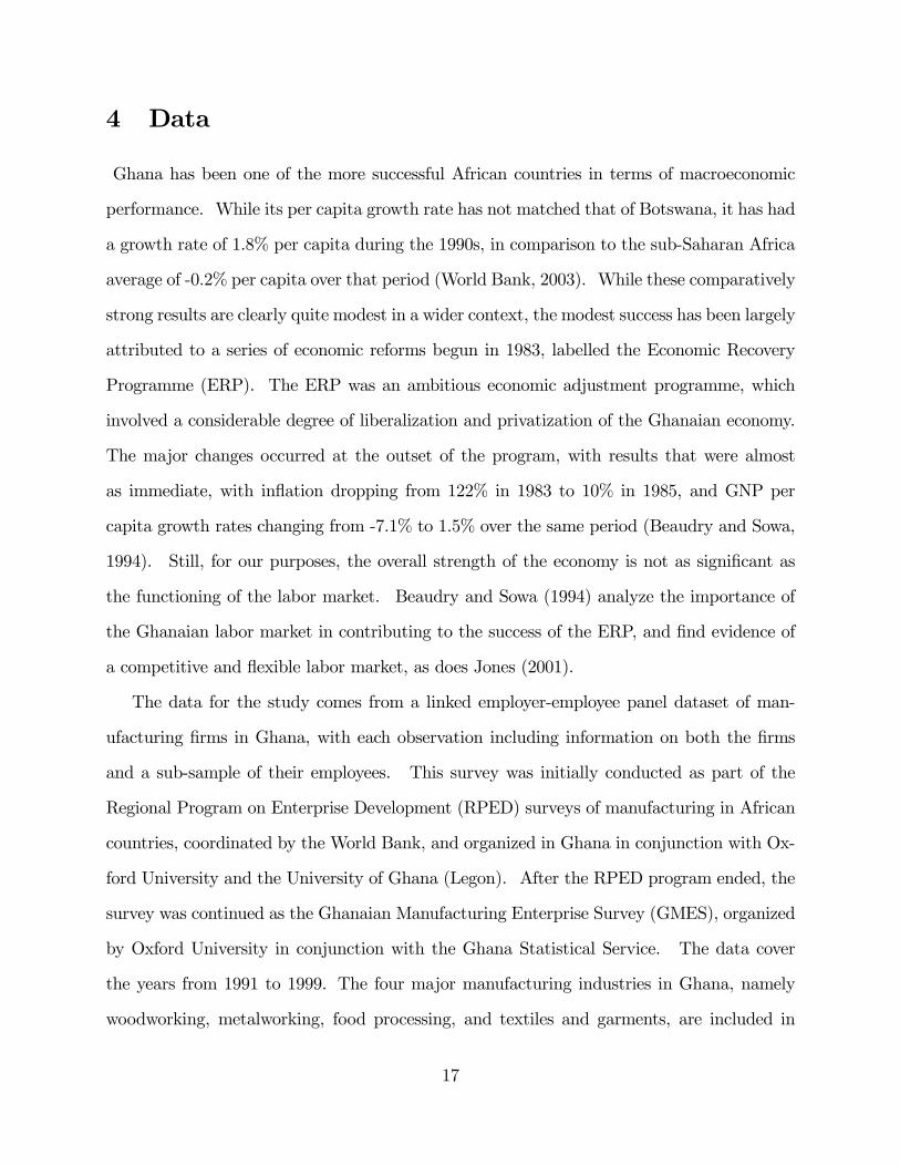
4 Data
Ghana has been one of the more successful African countries in terms of macroeconomic
performance. While its per capita growth rate has not matched that of Botswana, it has had
a growth rate of 1.8% per capita during the 1990s, in comparison to the sub-Saharan Africa
average of -0.2% per capita over that period (World Bank, 2003). While these comparatively
strong results are clearly quite modest in a wider context, the modest success has been largely
attributed to a series of economic reforms begun in 1983, labelled the Economic Recovery
Programme (ERP). The ERP was an ambitious economic adjustment programme, which
involved a considerable degree of liberalization and privatization of the Ghanaian economy.
The major changes occurred at the outset of the program, with results that were almost
as immediate, with inflation dropping from 122% in 1983 to 10% in 1985, and GNP per
capita growth rates changing from -7.1% to 1.5% over the same period (Beaudry and Sowa,
1994). Still, for our purposes, the overall strength of the economy is not as significant as
the functioning of the labor market. Beaudry and Sowa (1994) analyze the importance of
the Ghanaian labor market in contributing to the success of the ERP, and find evidence of
a competitive and flexible labor market, as does Jones (2001).
The data for the study comes from a linked employer-employee panel dataset of man-
ufacturing firms in Ghana, with each observation including information on both the firms
and a sub-sample of their employees. This survey was initially conducted as part of the
Regional Program on Enterprise Development (RPED) surveys of manufacturing in African
countries, coordinated by the World Bank, and organized in Ghana in conjunction with Ox-
ford University and the University of Ghana (Legon). After the RPED program ended, the
survey was continued as the Ghanaian Manufacturing Enterprise Survey (GMES), organized
by Oxford University in conjunction with the Ghana Statistical Service. The data cover
the years from 1991 to 1999. The four major manufacturing industries in Ghana, namely
woodworking, metalworking, food processing, and textiles and garments, are included in
17

the sample, and together they comprise 70 percent of manufacturing employment in Ghana
(CSAE and University of Ghana, 1994). The original sampling frame was the 1987 Census
of Manufacturing Activities in Ghana. For details on the sampling procedure, see CSAE
and University of Ghana (1994). Some exit and attrition from the sample occurred, and
these firms were replaced with firms of the same size category, sector, and location, so that
near (but not exactly) 200 firms were sampled in each year. Overall then, the dataset is an
unbalanced panel. Moreover, a sample of 10 workers at each firm was surveyed (or all of
the firm’s workers, in the case of fewer than 10 workers), thus creating the linked employer-
employee dataset, allowing the use of the techniques described in the methodology section.
Information on firm output prices and input costs are used to construct firm-level price and
input price deflators. Earnings are deflated using the consumer price index.
In addition to the GMES, the fourth round of the Ghana Living Standards Survey (GLSS
4), a nationally representative household survey (6000 households) in Ghana conducted
between April 1998 and March 1999, is also used in this study for comparison purposes for
the summary statistics. The third round of this data, GLSS 3, collected betwen 1991 and
1992, is used to calculate school tuition amounts. The returns to education calculated in
this paper should be interpreted as the returns to education within the manufacturing sector
in Ghana, although when we compare the characteristics of these (GMES) workers to wage
workers from the GLSS (in Appendix Table A1), we find similarities.
5 Results
The methodology in the previous section delineates the procedure for the case of the Mincer
specification of the wage equation. Heckman, Lochner, and Todd (2006) note that the
central functional form prediction of one version of Mincer’s model is that log-earnings
experience profiiles are parallel across schooling levels (and that log-earnings age profiles
diverge with age across schooling levels). They propose an empirical test for this, which we
18

also follow. Specifically, we nonparametrically estimate log-earnings experience profiles (for
men) for different education levels—none, primary, middle, and secondary, with the results
presented in Appendix Figure A1.24 First, we note that in comparison to their results,
the wage profiles are relatively flat across experience levels. Following Heckman, Lochner,
and Todd (2006), we test whether these log-earnings experience profiles are parallel across
schooling levels, with the results of this test in Appendix Table A2. Following the test,
we cannot reject at the 5% level that the lines are parallel, but can reject at the 10% level.
However, glancing at the nonparametric results in Appendix Figure A1, we see that a more
serious assumption that appears to be violated in the data is the assumption of linearity
in schooling. The difference in years of schooling between none and primary, primary and
middle, and middle and secondary is 6, 4, and 5 respectively, and yet clearly the returns to
secondary are higher than the other returns.25 In order to address this fact, a quadratic
functional form in education will be used in the estimation below.
The first step in our procedure to estimate consistently the returns to education involves
estimating the production function. The production function estimates are presented in
Table 1. The first two columns are the results of least-squares estimation, including or
omitting a gender control. In the OLS specification, the coefficients on the labor term,
education, and the capital term are precisely estimated, while the other labor coefficients
are not precisely estimated. The lack of significance on the experience terms is consistent
with the lack of a strong wage return to experience as noted in the nonparametric results.
The production function results of the ACF procedure for the base specification are provided
in columns (3) and (4), and for a quadratic specification are provided in columns (5) and
(6). The ACF procedure is designed to handle simultaneity in the production function.
Levinsohn and Petrin (2003) provide the conditions under which the least-squares labour
24The confidence intervals are bootstrapped, with b=300.25The number who have completed tertiary education is extremely small, 1% of the sample, insufficient
for the nonparametric analysis and tests. Therefore, this group has been dropped from the Mincer testingdescribed here, but not from any other calculations in the paper.
19

coefficient is upward-biased in a production function, and the least-squares capital coefficient
downward-biased, and we find some evidence for this in columns (3) through (6). The a
priori prediction is not as clear for the average education level of the workforce, and we
find that it does not differ significantly from the OLS results. Finally, a quadratic for
education is used in columns (5) and (6). The results for the non-education terms are fairly
similar. Also, the squared term of the education quadratic is only significant at the 10%
level, and only with the inclusion of the gender control. The linear education term ceases
to be significant.26
As noted previously, these coefficient estimates allow us to calculate the coefficients in the
skill production function (g). The skill production coefficients for schooling are calculated
and provided at the bottom of the table (βS and βV ). Here, the estimates suggest that,
in the linear case, an additional year of schooling increases one’s skill or human capital by
7.4%.
We can also compare the production function estimates of the skill production parameters
with those obtained in the wage equation, using the specification of (21) to control for
worker ability in the wage regressions. The benchmark results are provided in Table 2. As
previously mentioned, in order to make use of the measures of worker ability obtained from
the firm production functions, the regressions are all grouped regressions, which do provide
consistent (although inefficient) estimates of all parameters. Note that since the productivity
term has been generated in the first stage of the regression, the standard errors have been
bootstrapped. The first column presents the least-squares estimates, that is the grouped
regression version of equation (5), without the ability control. The second column presents
the results of estimating equation (21). The Mincer coefficient on the education term drops
from 0.104 to 0.074, in accord with the a priori expectations of most researchers. Columns
26Another specification that relaxes the Mincer linearity assumption is to use dummy variables for each ofthe categories of schooling in the Ghanaian context. This is also attempted, with the results in AppendixTable A3. Unfortunately, with the larger number of human capital coefficients, the coefficient estimates areimprecise, and so this specification is not used further.
20

(3) and (4) repeat the results of columns (1) and (2), but including a gender control, with
a similar estimate of 0.072 in the corrected version.27 In columns (5) and (6), we see that
the skill production coefficient on schooling estimated from the production function (0.074)
is very similar to the skill production coefficient on schooling in the wage equation (0.072),
although the bootstrapped standard error on the production function coefficient prevents
strong conclusions here.
In Table 3, we allow for a quadratic specification for education, using the results of
columns (5) and (6) of Table 1. Since the linear education specification of Table 2 is nested
in the quadratic specification of Table 3, technically the test of whether the quadratic speci-
fication is preferred to the linear specification is a test of the significance of the squared term
in the quadratic specification. This term is significant in each of the non-OLS specifica-
tions, and its presence forces the linear term to be insignificant. For comparison purposes,
when we calculate the internal rate of return to education, we will use both the linear and
quadratic specifications for education.
As previously noted, the education skill production coefficient from a Mincer regression
only represents the internal rate of return (IRR) to education under strict conditions. It is
still possible to use the coefficients on schooling from the regressions of Tables 2 and 3 to
calculate such an internal rate of return as the discount rate that equates lifetime earnings
streams for two different schooling levels. The tuition cost of schooling, as well as the tax
rate should be taken into account when making this calculation.28 That is, for the schooling
27Recall that the productivity variable varies according to the regression, depending on the regressorsincluded in the wage equation (and therefore in the corresponding production function). That is, theprocedure described earlier requires that the same variables are included in the production function as inthe wage equation, in order to capture the appropriate measure of productivity.28In fact, Heckman, Lochner and Todd (2006) generalize even this specification to also account for un-
certainty, and agent expectation formation. In addition, they find that once one allows for the sequentialresolution of uncertainty, unique internal rates of return to education are no longer guaranteed. Theiranalysis certainly suggests the fruitfulness of a more general analysis of the value of education. However,just as Heckman, Lochner and Todd (2006) abstract from the issue of ability bias in order to introduce theseimportant issues, this paper will abstract from the issue of sequential resolution of uncertainty to focus onthe ability bias issue. Future research will seek to merge the two. Calculating a more robust IRR, thepurpose of this paper, is an important first step, particularly in the developing country context.
21
levels s1 and s2, the internal rate of return rI(s1, s2) solves the equation:
[T (s1)−s1]R0
(1− τ)e−rI(x+s1)w(s1, x)dx−s1R0
v(z)e−rIzdz(22)
=[T (s2)−s2]R
0
(1− τ)e−rI(x+s2)w(s2, x)dx−s2R0
v(z)e−rIzdz
where tuition costs of schooling level z are captured in v(z), taxes in τ , the length of a
worklife with s years of schooling in T (s), and the wage with schooling s and experience x
captured in w(s, x). The wage data in our survey measures after-tax wages, and so we do not
need to explicitly include the taxation rate.29 While data on school tuition is not collected
in the GMES survey, we use the GLSS 3 survey30 to calculate the average amount of money
spent on an individual’s student’s education in Ghana, at various education levels.31 This
amount is calculated as a separate average for primary school, middle school, secondary
school, and tertiary education. We calculate a discretized version of the education of
equation (22). The results are presented in Table 4, under the assumption of an earning life
of 42 years, which is consistent with the life expectancy in Ghana in the early 1990s. For
the linear case, we see that the OLS results overestimate the returns to education by roughly
3 percent in comparison to our preferred results. On the other hand, when the quadratic in
education is used, we see higher returns for higher levels of education. Moreover, correcting
for ability bias makes a large difference (5 versus 9 percent) at lower levels of education,
but a smaller difference (12 versus 13 percent) at higher levels of education. An important
caveat should accompany this conclusion. In this specification, education is allowed to have
a non-linear (quadratic) impact on the wage, while ability is restricted to be linear, given the
29Income taxes are only an issue for those firms within the formal sector. For firms in the informal sector,workers’ incomes are not taxed. In either case, we have a measure of the income taken home by the worker.30The GLSS 3 Survey was conducted between September 1991 and September 1992. This survey is used,
rather than the GLSS 4 because this survey is earlier, and therefore closer to the time when the workforceunder examination (or more specifically their parents) would having been making schooling decisions, basedon future expectations of schooling’s value. All values are converted to 1991 cedis for the purpose of thesecalculations.31This totals the amount spent on school and registration fees, contributions to parent/teacher associations,
school uniforms, books and school supplies, transportation to and from school, food and lodging at the school(if applicable), and other cash and in-kind school expenses.
22
methodology. While technically speaking, ability could enter in a non-linear (e.g. quadratic)
fashion in the wage equation, and therefore into the production function, only the composite
ability term (the combined linear plus squared term of the quadratic) could be isolated in
the left-hand-side of equation (17) in this procedure, in essence restricting the impact of
ability to being linear. The conclusions on the IRR quadratic should be interpreted with
this caveat in mind.
Further robustness checks on the estimation are performed in Appendix Table A4, which
includes firm size as an additional regressor in the wage equation. The basic magnitude
and direction of the results does not change. The estimated coefficient on the education
term in the preferred specification with and without a gender control are 0.075 and 0.072,
respectively, which is very similar to the earlier results of 0.074 and 0.072 for both preferred
specifications of Table 2.
As mentioned previously, the wage equation has been estimated as a grouped regression,
grouping at the level of the firm, based on a sub-sample of workers at each firm. This will
create measurement error in the worker variables in the production function (although it
should be noted that this measurement error is considerably preferred to the omitted variable
bias that usually exists with the omission of these variables). As a result, it will also create
measurement error in the productivity variable for use in the wage regression. The fact that
not all of the workers at a firm are surveyed technically also affects the measurement of the
worker variables in the wage regression, although since the wage is calculated from the same
subset of workers, this is not the primary issue on the worker variables.
To address these issues, the analysis is re-done on the set of firms with 20 or fewer
employees. The measurement error issue should be drastically improved for this set of
firms.32 These results are presented in Table 5. In all cases, we see that measurement
error on the productivity variable did appear to be an issue, as the productivity coefficient
32The analysis was also performed on firms with 10 or fewer employees, for which sample-related measure-ment error is not an issue, and there was very little difference from the 20 or fewer results.
23
increases considerably. We also see that the linear education coefficient is roughly 0.01
larger in all specifications, in both OLS and preferred specifications. This suggests that the
measurement error affected roughly all specifications symmetrically. Of course, it is also
possible that the returns to education are merely different in these smaller firms. In Table 6,
we calculate the internal rates of return for the workers of these small firms. The results are
very similar to those of Table 4. Again, in the linear specification, the OLS results overstate
the returns to education by roughly 3 percent. In the quadratic specification, we again see
that correcting for ability bias matters more at the lower and middle levels of education than
it does at upper levels, subject to the caveat mentioned earlier.
6 Conclusion
This paper has demonstrated a new method for estimating the coefficients in a wage equa-
tion, which are typically interpreted as the skill production or human capital production
coefficients in a competitive market for skill. The approach is to consider the use of skill
from the firm’s perspective, and to measure the productive returns of these characteristics
in a firm production function. This paper has developed (and proved) the unique form
for the labor term in the production function that is consistent with a general form of the
wage equation. In addition to estimating the skill production parameters directly in a firm
production function, the paper has demonstrated that we can also use information captured
in the production function estimation in order to consistently estimate parameters in a wage
equation. Specifically, we find that an estimate of worker ability is retrievable from the
production function estimation, and this measure of worker ability can be used to control
directly for worker ability in a wage regression. This should not be surprising. Firm pro-
ductivity in essence captures the productive differences of firms that have similar observable
characteristics, such as the number of workers, the size of the capital stock, and the average
schooling of the workforce. Certainly, part of these differences in firm productivity reflect
24
differences in worker ability.
The methodology used in this paper, while obtaining a measure of worker ability from the
structural industrial organization literature, was closer in procedure to the non-structural
returns to education literature. In much of the non-structural (IV) literature, the preferred
estimates are frequently larger than the OLS estimates. Card (1999, 2001) and Heckman,
Lochner and Todd (2006) offer discussions of why the IV estimates might be above the OLS
estimates. In contrast, the structural estimates of returns to education for the population as
a whole are frequently lower than the OLS estimates. Here, by using a novel procedure for
controlling for ability bias that differs considerably from the structural methods currently
used, we also find an ability bias that is in the upward direction.
Specifically, the preferred results from the wage equation estimation procedure (which are
found to be similar to the production function estimates) suggest a linear schooling coefficient
of 0.080, in comparison to the OLS coefficient of 0.100 (in the small firms, least affected by
measurement error), with a corresponding average internal rate of return of roughly 7%.
However, the results also suggest that the returns to education increase with the level of
education in Ghana. Using a quadratic specification, we find that ability bias continues
to matter, is on average roughly 3 percent, although ability bias also appears higher at the
lower levels of education, where the returns are also lower.
For the Ghanaian context, an additional point should be made. The returns to education
appear to be considerably higher for secondary than for primary levels. Of course, primary
education is an input into secondary education. These results seem to suggest that the
returns to primary education reflect its role as an input at least as much as its direct con-
tribution to earnings, at least in the Ghanaian manufacturing sector, although the returns
to primary education do remain non-trivial, at at least 5%, after accounting for the cost of
such an education.
Fortunately, the recent expansion in the availability of linked employer-employee datasets
25

has increased the potential to use firm information to answer a wide variety of questions
related to workers. In fact, labor economists have been the first to make extensive use of
these linked datasets to examine questions of interest to them. However, linked datasets
are also of use to those studying the firm. This paper has demonstrated the means by
which the a generic wage equation can be made consistent with, and incorporated into, the
production function of the firm. While this technique should expand the potential areas
of inquiry, hopefully it will spark further research into the best use of information about a
firm’s workers, in terms of its contribution to the understanding of the firm as well.
26
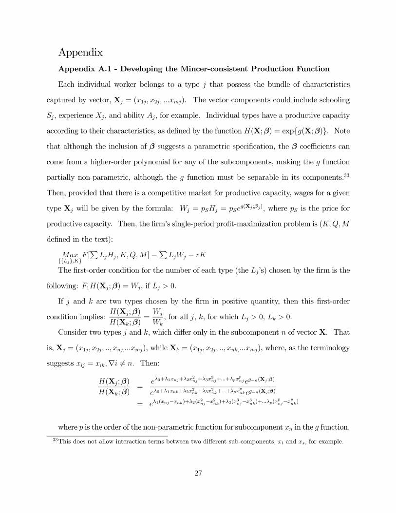
AppendixAppendix A.1 - Developing the Mincer-consistent Production Function
Each individual worker belongs to a type j that possess the bundle of characteristics
captured by vector, Xj = (x1j, x2j, ...xmj). The vector components could include schooling
Sj, experience Xj, and ability Aj, for example. Individual types have a productive capacity
according to their characteristics, as defined by the functionH(X;β) = exp{g(X;β)}. Notethat although the inclusion of β suggests a parametric specification, the β coefficients can
come from a higher-order polynomial for any of the subcomponents, making the g function
partially non-parametric, although the g function must be separable in its components.33
Then, provided that there is a competitive market for productive capacity, wages for a given
type Xj will be given by the formula: Wj = pSHj = pSeg(Xj ;βj), where pS is the price for
productive capacity. Then, the firm’s single-period profit-maximization problem is (K,Q,M
defined in the text):
Max{{Lj},K}
F [P
LjHj,K,Q,M ]−PLjWj − rK
The first-order condition for the number of each type (the Lj’s) chosen by the firm is the
following: F1H(Xj;β) =Wj, if Lj > 0.
If j and k are two types chosen by the firm in positive quantity, then this first-order
condition implies:H(Xj;β)
H(Xk;β)=
Wj
Wk, for all j, k, for which Lj > 0, Lk > 0.
Consider two types j and k, which differ only in the subcomponent n of vector X. That
is, Xj = (x1j, x2j, .., xnj,...xmj), while Xk = (x1j, x2j, .., xnk,...xmj), where, as the terminology
suggests xij = xik,∇i 6= n. Then:
H(Xj;β)
H(Xk;β)=
eλ0+λ1xnj+λ2x2nj+λ3x
3nj+...+λpx
pnjeg−n(Xj ;β)
eλ0+λ1xnk+λ2x2nk+λ3x
3nk+...+λpx
pnkeg−n(Xj ;β)
= eλ1(xnj−xnk)+λ2(x2nj−x2nk)+λ3(x3nj−x3nk)+...λp(xpnj−xpnk)
where p is the order of the non-parametric function for subcomponent xn in the g function.
33This does not allow interaction terms between two different sub-components, xi and xs, for example.
27
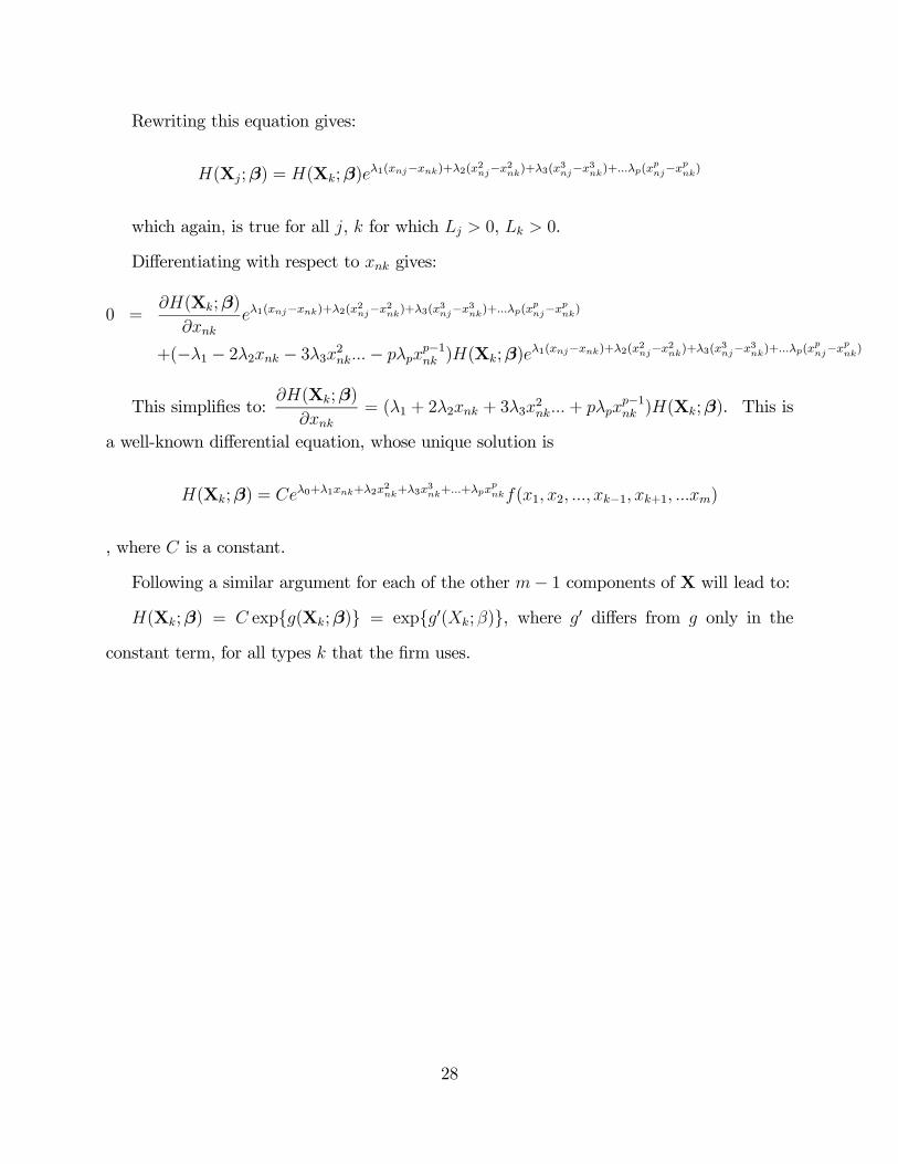
Rewriting this equation gives:
H(Xj;β) = H(Xk;β)eλ1(xnj−xnk)+λ2(x2nj−x2nk)+λ3(x3nj−x3nk)+...λp(xpnj−xpnk)
which again, is true for all j, k for which Lj > 0, Lk > 0.
Differentiating with respect to xnk gives:
0 =∂H(Xk;β)
∂xnkeλ1(xnj−xnk)+λ2(x
2nj−x2nk)+λ3(x3nj−x3nk)+...λp(xpnj−xpnk)
+(−λ1 − 2λ2xnk − 3λ3x2nk...− pλpxp−1nk )H(Xk;β)e
λ1(xnj−xnk)+λ2(x2nj−x2nk)+λ3(x3nj−x3nk)+...λp(xpnj−xpnk)
This simplifies to:∂H(Xk;β)
∂xnk= (λ1 + 2λ2xnk + 3λ3x
2nk... + pλpx
p−1nk )H(Xk;β). This is
a well-known differential equation, whose unique solution is
H(Xk;β) = Ceλ0+λ1xnk+λ2x2nk+λ3x
3nk+...+λpx
pnkf(x1, x2, ..., xk−1, xk+1, ...xm)
, where C is a constant.
Following a similar argument for each of the other m− 1 components of X will lead to:
H(Xk;β) = C exp{g(Xk;β)} = exp{g0(Xk;β)}, where g0 differs from g only in the
constant term, for all types k that the firm uses.
28
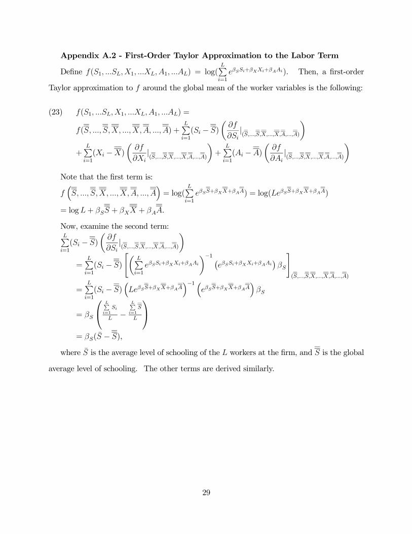
Appendix A.2 - First-Order Taylor Approximation to the Labor Term
Define f(S1, ...SL,X1, ...XL, A1, ...AL) = log(LPi=1
eβSSi+βXXi+βAAi). Then, a first-order
Taylor approximation to f around the global mean of the worker variables is the following:
f(S1, ...SL, X1, ...XL, A1, ...AL) =(23)
f(S, ..., S,X, ..., X,A, ..., A) +LPi=1
(Si − S)
µ∂f
∂Si|(S,...,S,X,...,X,A,...,A)
¶+
LPi=1
(Xi −X)
µ∂f
∂Xi|(S,...,S,X,...,X,A,...,A)
¶+
LPi=1
(Ai −A)
µ∂f
∂Ai|(S,...,S,X,...,X,A,...,A)
¶Note that the first term is:
f³S, ..., S,X, ..., X,A, ..., A
´= log(
LPi=1
eβSS+βXX+βAA) = log(LeβSS+βXX+βAA)
= logL+ βSS + βXX + βAA.
Now, examine the second term:LPi=1
(Si − S)
µ∂f
∂Si|(S,...,S,X,...,X,A,...,A)
¶=
LPi=1
(Si − S)
"µLPi=1
eβSSi+βXXi+βAAi
¶−1 ¡eβSSi+βXXi+βAAi
¢βS
#(S,...,S,X,...,X,A,...,A)
=LPi=1
(Si − S)³LeβSS+βXX+βAA
´−1 ³eβSS+βXX+βAA
´βS
= βS
⎛⎝ LPi=1
Si
L−
LPi=1
S
L
⎞⎠= βS(S̄ − S),
where S̄ is the average level of schooling of the L workers at the firm, and S is the global
average level of schooling. The other terms are derived similarly.
29
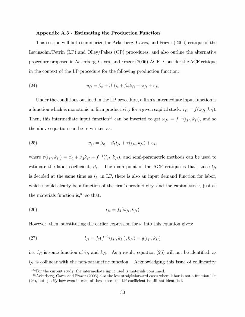
Appendix A.3 - Estimating the Production Function
This section will both summarize the Ackerberg, Caves, and Frazer (2006) critique of the
Levinsohn/Petrin (LP) and Olley/Pakes (OP) procedures, and also outline the alternative
procedure proposed in Ackerberg, Caves, and Frazer (2006)-ACF. Consider the ACF critique
in the context of the LP procedure for the following production function:
(24) yft = β0 + β1lft + β2kft + ωft + εft
Under the conditions outlined in the LP procedure, a firm’s intermediate input function is
a function which is monotonic in firm productivity for a given capital stock: ift = f(ωft, kft).
Then, this intermediate input function34 can be inverted to get ωft = f−1(ift, kft), and so
the above equation can be re-written as:
(25) yft = β0 + β1lft + τ(ift, kft) + εft
where τ(ift, kft) = β0 + β2kft + f−1(ift, kft), and semi-parametric methods can be used to
estimate the labor coefficient, βl. The main point of the ACF critique is that, since lft
is decided at the same time as ift in LP, there is also an input demand function for labor,
which should clearly be a function of the firm’s productivity, and the capital stock, just as
the materials function is,35 so that:
(26) lft = f2(ωft, kft)
However, then, substituting the earlier expression for ω into this equation gives:
(27) lft = f2(f−1(ift, kft), kft) = g(ift, kft)
i.e. lft is some function of ift and kft. As a result, equation (25) will not be identified, as
lft is collinear with the non-parametric function. Acknowledging this issue of collinearity,
34For the current study, the intermediate input used is materials consumed.35Ackerberg, Caves and Frazer (2006) also the less straightforward cases where labor is not a function like
(26), but specify how even in each of these cases the LP coefficient is still not identified.
30

ACF recognize that the production function can be re-written as:
(28) yft = φ(ift, kft, lft) + εft
where φ(ift, kft) = τ(ift, kft, lft)+ g(ift, kft), allowing for the possibility that labor is chosen
at some time t − b, 0 < b < 1, between the choice of capital (t − 1) and the choice ofintermediate inputs (t).36 Therefore, in the first stage of ACF estimation, no coefficients
are identified, just the φ function.37 Then, each of the relevant coefficients is estimated in
the second stage of estimation using appropriate moment conditions, as outlined presently.
As in both OP and LP, ACF assume that the productivity term follows a first-order Markov
process:
(29) ωft = E[ωft|ωft−1] + ξft
As in both OP and LP, for ACF, the current period’s capital stock is assumed to be
determined by investment in the previous period, so that the unexpected innovation in
productivity is orthogonal to the current period’s capital stock:
(30) E[ξft|kft] = 0
To construct the empirical analogue of this moment, ACF use the following expression,
working from equation (29):
(31)
ξft(βk, βl) = ωft(βk, βl)−E[ωft|ωft−1;βk, βl] = (cφft−βkkft−βllft)−bψ(βk, βl, dφft−1, kft−1, lft−1)As mentioned, values of cφft are obtained in the first stage of estimation, and the bψ
terms are predicted values from a non-parametric regression of (cφft − βkkft − βllft) on
(dφft−1 − βkkft−1 − βllft−1). A second moment condition is required (as there are two
36Note that another assumption in this method (and that of OP and LP) is that the input prices areassumed constant across firms for the period of estimation of a given φ function (the entire period in ourdataset), and so these prices do not need to be entered directly into the input demand functions.37The nonparametric estimation method used is a Nadaraya-Watson local-constant-least-squares estimator
with a normal kernel, and an optimal bandwidth.
31
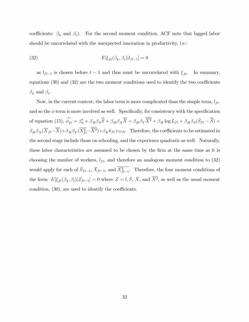
coefficients: βk and βl). For the second moment condition, ACF note that lagged labor
should be uncorrelated with the unexpected innovation in productivity, i.e.:
(32) E[ξft(βk, βl)|lft−1] = 0
as lft−1 is chosen before t − 1 and thus must be uncorrelated with ξft. In summary,
equations (30) and (32) are the two moment conditions used to identify the two coefficients
βk and βl.
Now, in the current context, the labor term is more complicated than the simple term, lft.
and so the φ term is more involved as well. Specifically, for consistency with the specification
of equation (15), cφft = β∗0 + βHβSS + βHβXX + βHβYX2 + βH logLft + βHβS(S̄ft − S) +
βHβX(Xft−X)+βHβY (X2ft−X2)+βKkft+ωft. Therefore, the coefficients to be estimated in
the second stage include those on schooling, and the experience quadratic as well. Naturally,
these labor characteristics are assumed to be chosen by the firm at the same time as it is
choosing the number of workers, lft, and therefore an analogous moment condition to (32)
would apply for each of S̄ft−1, X̄ft−1, and X2ft−1. Therefore, the four moment conditions of
the form: E[ξft(βk, βl)|Zft−1] = 0 where Z = l, S̄, X̄, and X2, as well as the usual moment
condition, (30), are used to identify the coefficients.
32
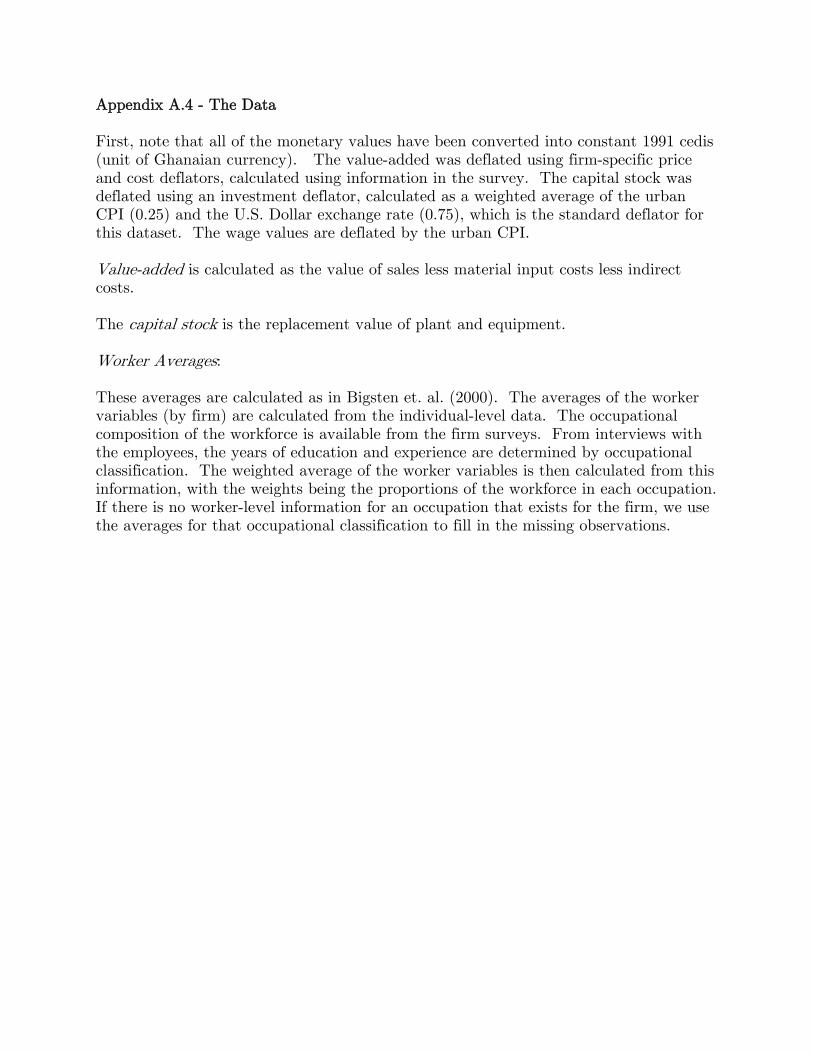
Appendix A.4 - The Data First, note that all of the monetary values have been converted into constant 1991 cedis (unit of Ghanaian currency). The value-added was deflated using firm-specific price and cost deflators, calculated using information in the survey. The capital stock was deflated using an investment deflator, calculated as a weighted average of the urban CPI (0.25) and the U.S. Dollar exchange rate (0.75), which is the standard deflator for this dataset. The wage values are deflated by the urban CPI. Value-added is calculated as the value of sales less material input costs less indirect costs. The capital stock is the replacement value of plant and equipment. Worker Averages: These averages are calculated as in Bigsten et. al. (2000). The averages of the worker variables (by firm) are calculated from the individual-level data. The occupational composition of the workforce is available from the firm surveys. From interviews with the employees, the years of education and experience are determined by occupational classification. The weighted average of the worker variables is then calculated from this information, with the weights being the proportions of the workforce in each occupation. If there is no worker-level information for an occupation that exists for the firm, we use the averages for that occupational classification to fill in the missing observations.
References
Abowd, J. M. and Kramarz, F. (1999), “The Analysis of Labor Markets Using MatchedEmployer-Employee Data”, in O. Ashenfelter and D. Card (eds.), Handbook of Labor Eco-nomics, Vol. 3B (New York: Elsevier Science, North-Holland).
Ackerberg, D. A., Caves, K., and Frazer, G. (2006), “Structural Estimation of ProductionFunctions,” mimeo, University of Toronto and UCLA.
Alderman, H., Behrman, J.R., Khan, S., Ross, D.R., and Sabot, R. (1997), “The IncomeGap in Cognitive Skills in Rural Pakistan,” Economic Development and Cultural Change,46, pp. 97-122.
Alderman, H., Behrman, J.R., Ross, D.R., and Sabot, R. (1996), “The Returns to En-dogenous Human Capital in Pakistan’s Rural Wage Labour Market,” Oxford Bulletin ofEconomics and Statistics, 58, pp. 29-55.
Angrist, Joshua D. and Imbens, Guido W. (1994), “Identification and Estimation of LocalAverage Treatment Effects,” Econometrica, 62(2), March, pp. 467-475.
Angrist, Joshua D. and Krueger, A. B. (1991) “Does Compulsory School Attendance AffectSchooling and Earnings?” Quarterly Journal of Economics, 106, November, pp. 979-1014.
Appleton, S., Hoddinnott, J. and MacKinnon, J. (1996), “Education and Health in Sub-Saharan Africa”, Journal of International Development, 8, 307-339.
Ashenfelter, Orley and Zimmerman, D. (1997), “Estimates of the Return to Schooling fromSibling Data: Fathers, Sons and Brother,” Review of Economics and Statistics, 79, pp. 1-9.
Beaudry, P. and Sowa, N. K. (1994), “Ghana”, in S. Horton, R. Kanbur, and D. Mazumdar,(eds.), Labor markets in an era of adjustment, Vol. 2. (Washington, D.C.: World Bank).
Becker, G. S. (1964) Human Capital: A Theoretical and Empirical Analysis, with SpecialReference to Education (New York: Columbia University Press).
Behrman, J. R. (1996), “Human Capital Formation, Returns and Policies: Analytical Ap-proaches and Research Questions”, Journal of International Development, 8, 341-373.
Behrman, J. R., Foster, A. D., Rosenzweig, M. R. and Vashishtha, P. (1999), “Women’sSchooling, Home Teaching, and Economic Growth”, Journal of Political Economy, 107, 682-714.
Behrman, J. R. and Deolalikar, A. B. (1991), “School Repetition, Dropouts, and the Ratesof Return to Schooling: the Case of Indonesia”, Oxford Bulletin of Economics and Statistics,53, 467-480.
Belzil, C. (2007) “The Return to Schooling in Structural Dynamic Models: A Survey,”European Economic Review, 51, 1059-1105.
34
Belzil, C. and Hansen, J. (2007) “A Structural Analysis of the Correlated Random CoefficientWage Regression Model,” Journal of Econometrics, in press.
Belzil, C. and Hansen, J. (2002), “Unobserved Ability and the Return to Schooling,” Econo-metrica, 70(5), 2075-2091.
Bigsten, A., Collier, P., Dercon, S., Fafchamps, M., Gauthier, B., Gunning, J. W., Isaksson,A., Oduro, A., Oostendorp, R., Patillo, C., Soderbom, M., Teal, F., and Zeufack, A. “Con-tract Flexibility and Dispute Resolution in African Manufacturing”, Journal of DevelopmentStudies, 36, 1-17.
Bils, M. R. and Klenow, P. J. (2000), “Does Schooling Cause Growth?” American EconomicReview, 90, 1160-1183.
Boissiere, M., Knight, J. B. and Sabot, R. H. (1985), “Earnings, Schooling, Ability, andCognitive Skills”, American Economic Review, 75, 1016-1030.
Brunello, G., and Miniaci, R. (1999), “The Economic Returns to Schooling for Italian Men.An Evaluation Based on Instrumental Variables,” Labour Economics, 6, pp. 509-519.
Callan, T. and Harmon, C., (1999), “The Economic Return to Schooling in Ireland,” LabourEconomics, 6, pp. 543-550.
Card, D. (2001), “Estimating the Return to Schooling: Progress on Some Persistent Econo-metric Problems”, Econometrica, 69, 1127-1160.
Card, D. (1999) “The Causal Effect of Education on Earnings”, in O. Ashenfelter and D.Card (eds.), Handbook of Labor Economics, Vol. 3 (New York: Elsevier Science).
Card, D. (1995) “Earnings, Schooling, and Ability Revisited”, in S. W. Polachek (ed.),Research in Labor Economics, Vol. 14 (Greenwich, Conn.: JAI Press).
Centre for the Study of African Economies (CSAE) - University of Oxford and University ofGhana, “The Ghanaian Manufacturing Sector 1991-92: Findings of Waves 1 and 2” (WorldBank RPED paper #029).
Duflo, E. (2001), “Schooling and Labor Market Consequences of School Construction inIndonesia: Evidence from an Unusual Policy Experiment.” American Economic Review, 91,795-813.
Glewwe, P. (1999) The Economics of School Quality Investments in Developing Countries:An Empirical Study of Ghana (Houndmills, U.K.: Macmillan Press).
Glewwe, P. (1996), “The Relevance of Standard Estimates of Rates of Return to Schooling forEducation Policy: A Critical Assessment”, Journal of Development Economics, 51, 267-290.
Godana, T. (1997), “Returns to Education in the Manufacturing Sector in Zimbabwe: SomeEmpirical Evidence”, South African Journal of Economics, 65, 99-113.
35
Griliches, Z. (1977), “Estimating the Returns to Schooling: Some Econometric Problems.”Econometrica, 45, 1-22.
Griliches, Z. (1976), “Wages of Very Young Men”, Journal of Political Economy, 1976, 84,Part 2, pp. S69-S86.
Griliches, Z. and Mairesse, J. (1998), “Production Functions: The Search for Identification”,in S. Strøm (ed.), Econometrics and Economic Theory in the Twentieth Century: The RagnarFrisch Centennial Symposium (Cambridge, UK: Cambridge University Press).
Griliches, Z. andMason, W. M. (1972), “Education, Income and Ability”, Journal of PoliticalEconomy, 80, Part 2, S74-S103.
Harmon, C. and Walker, I. (1995), “Estimating the Economic Return to Schooling for theUnited Kingdom,” American Economic Review, 85, p. 1278-1286.
Heckman, J., Lochner, L., and Todd, P. (2006), “Earnings Functions, Rates of Return andTreatment Effects: The Mincer Equation and Beyond,” in Eric A. Hanushek nad FinishWelch, eds., Handbook of the Economics of Education, vol. 1. (Amsterdam: Elsevier North-Holland).
Heckman, James and Polachek, Solomon. (1974), “Empirical Evidence on the FunctionalForm of the Earnings-Schooling Relationship,” Journal of the American Statistical Associa-tion, 69 (346), June, pp. 350-354.
Hellerstein, J. K., Neumark, D. and Troske, K. R. (1999), “Wages, Productivity, and WorkerCharacteristics: Evidence from Plant-Level Production Functions and Wage Functions.”Journal of Labor Economics, 17, 409-446.
Imbens, G. and Angrist, J. (1994), “Identification and estimation of local average treatmenteffects,” Econometrica, 62, 467-476.
Jones, P. (2001), “Are Educated Workers Really More Productive?” Journal of DevelopmentEconomics, 64, 57-79.
Kane, T. J. and Rouse, C. E. (1993), “LaborMarket Returns to Two- and Four-Year Colleges:Is a Credit a Credit and Do Degrees Matter?” NBER Working Paper #4268, Cambridge,MA, pp. 46.
Keane, Michael P. and Wolpin, Kenneth I. (1997). “The Career Decisions of Young Men,”Journal of Political Economy, 105(3), pp. 473-522.
Knight, J. B. and Sabot, R. H. (1990) Education, Productivity, and Inequality: The EastAfrican Natural Experiment (New York: Oxford University Press).
Lassibille, G. and Tan, Jee-Peng. (2005) “The Returns to Education in Rwanda,” Journalof African Economics, 14(1), 92-116.
36
Levin, J. and Plug, Erik J.S. (1999) “Instrumenting Education and the Returns to Schoolingin the Netherlands,” Labour Economics, 6, pp. 521-534.
Levinsohn, J. and Petrin, A. (2003), “Estimating Production Functions Using Inputs toControl for Unobservables”, Review of Economic Studies, 70, 317-341.
Li, T. and Zhang, J. (1998), “Returns to Education under Collective and Household Farmingin China”, Journal of Development Economics, 56, 307-335.
Lucas, R. E., Jr. (1988), “On the Mechanics of Economic Development”, Journal of Mone-tary Economics, 22, 3-42.
Marschak, J. and Andrews W. H., Jr. “Random Simultaneous Equations and the Theory ofProduction”, Econometrica, 12, 143-205.
Mincer, J. (1974) Schooling, Experience, and Earnings (New York: National Bureau ofEconomic Research).
Mundlak, Y. (1961) "Empirical Production Function Free of Management Bias." Journal ofFarm Economics, 43(1), 44-56.
Mwabu, G. and Schultz, T. P. (1996) “Education Returns Across Quantiles of the WageFunction: Alternative Explanations for Returns to Education by Race in South Africa”,American Economic Review - Papers and Proceedings, 86, 335-339.
Nehru, V., Swanson, E. and Dubey, A. (1995), “A New Database on Human Capital Stockin Developing and Industrial Countries: Sources, Methodology, and Results”, Journal ofDevelopment Economics, 46, 379-401.
Nielsen, H. S. and Westergård-Nielsen, N. (2001), “Returns to Schooling in Less DevelopedCountries: New Evidence from Zambia”, Economic Development and Cultural Change, 49,364-394.
Olley, S. and Pakes, A. (1996), “The Dynamics of Productivity in the TelecommunicationsEquipment Industry”, Econometrica, 64, 1263-97.
Pritchett, Lant. (2001), “Where Has All the Education Gone?” World Bank Economic Re-view, 15(3), 367-391.
Ram, R. and Singh, R. D. (1988), “Farm Households in Rural Burkina Faso: Some Evi-dence on Allocative and Direct Return to Schooling, and Male-Female Labor ProductivityDifferentials”, World Development, 16, 419-424.
Romer, P. M. (1986), “Increasing Returns and Long-Run Growth”, Journal of PoliticalEconomy, 94, 1002-37.
Siphambe, H. K. (2000), “Rates of Return to Education in Botswana”, Economics of Edu-cation Review, 19, 291-300.
37
Söderbom, M., Teal, F., Wambugu, A., and Kahyarara, G. (2006), “The Dynamics of Returnsto Education in Kenyan and Tanzanian Manufacturing,” Oxford Bulletin of Economics andStatistics, 68(3), 261-288.
Smith, P. A. and Metzger, M. R. (1998), “The Return to Education: Street Vendors inMexico”, World Development, 26, 289-296.
Teal, F. (1996), “The Size and Sources of Economic Rents in a Developing Country Manu-facturing Labour Market,” Economic Journal 106 (July), 963-976.
Temple, J. R. (2001), “Generalizations that Aren’t? Evidence on Education and Growth”,European Economic Review, 45, 905-918.
Wolpin, Kenneth. (2003), “Wage Equations and Education Policy,” in Mathias Dewatripont,Lars P. Hansen and Stephen J. Turnovsky, eds., Advances in Economics and Econometrics:Theory and Applications: Eighth World Congress, Volume II. Cambridge, UK: CambridgeUniversity Press.
World Bank (2003) African Development Indicators (Washington, D.C.: World Bank).
38
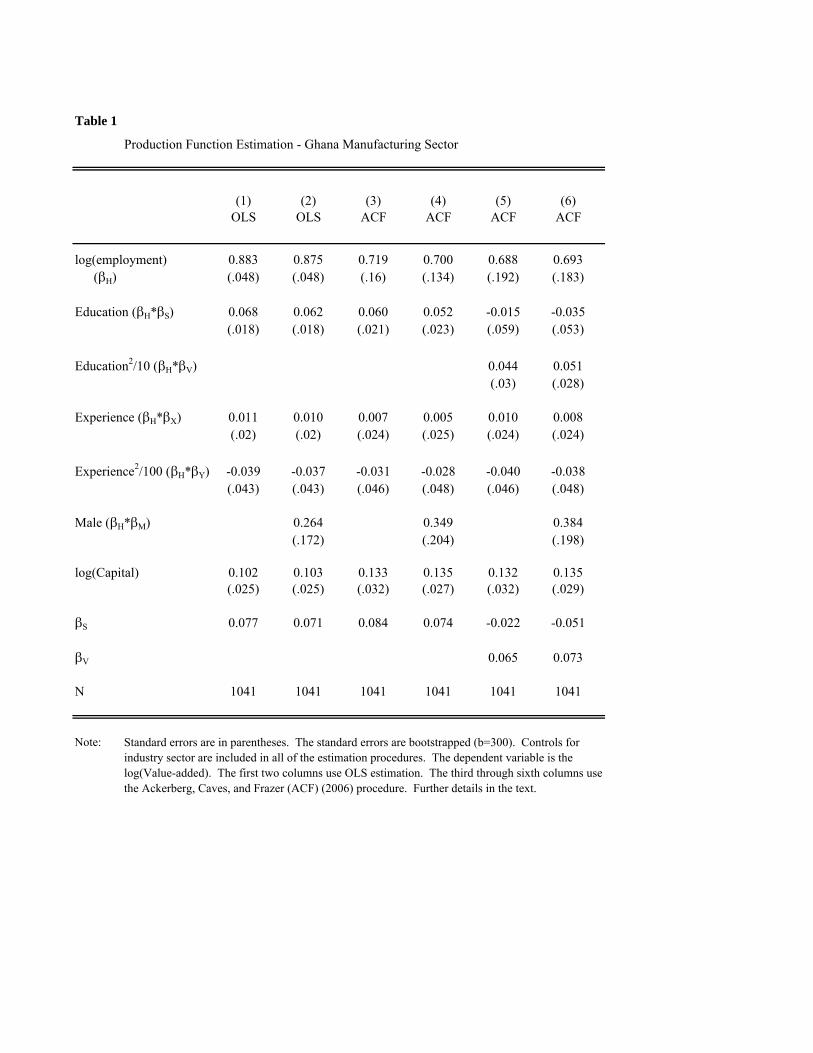
Table 1
Production Function Estimation - Ghana Manufacturing Sector
(1) (2) (3) (4) (5) (6)OLS OLS ACF ACF ACF ACF
log(employment) 0.883 0.875 0.719 0.700 0.688 0.693(βH) (.048) (.048) (.16) (.134) (.192) (.183)
Education (βH*βS) 0.068 0.062 0.060 0.052 -0.015 -0.035(.018) (.018) (.021) (.023) (.059) (.053)
Education2/10 (βH*βV) 0.044 0.051(.03) (.028)
Experience (βH*βX) 0.011 0.010 0.007 0.005 0.010 0.008(.02) (.02) (.024) (.025) (.024) (.024)
Experience2/100 (βH*βY) -0.039 -0.037 -0.031 -0.028 -0.040 -0.038(.043) (.043) (.046) (.048) (.046) (.048)
Male (βH*βM) 0.264 0.349 0.384(.172) (.204) (.198)
log(Capital) 0.102 0.103 0.133 0.135 0.132 0.135(.025) (.025) (.032) (.027) (.032) (.029)
βS 0.077 0.071 0.084 0.074 -0.022 -0.051
βV 0.065 0.073
N 1041 1041 1041 1041 1041 1041
Note: Standard errors are in parentheses. The standard errors are bootstrapped (b=300). Controls for industry sector are included in all of the estimation procedures. The dependent variable is the log(Value-added). The first two columns use OLS estimation. The third through sixth columns use the Ackerberg, Caves, and Frazer (ACF) (2006) procedure. Further details in the text.
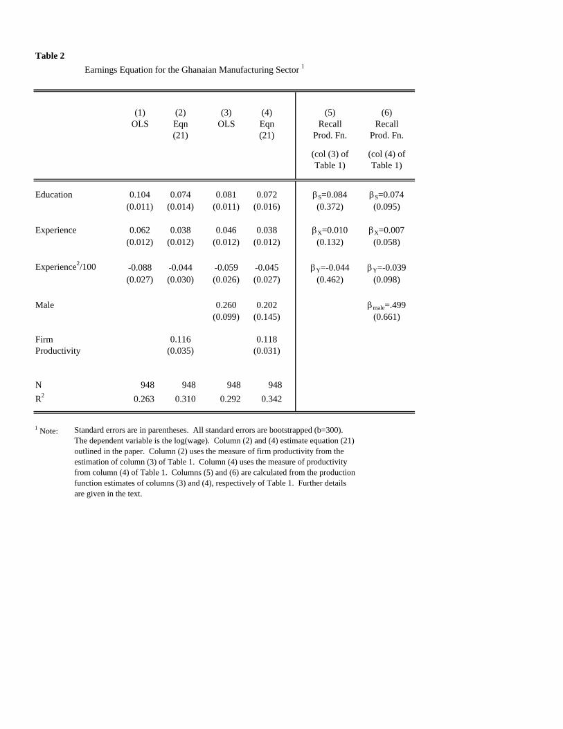
Table 2Earnings Equation for the Ghanaian Manufacturing Sector 1
(1) (2) (3) (4) (5) (6)OLS Eqn OLS Eqn Recall Recall
(21) (21) Prod. Fn. Prod. Fn.
(col (3) of (col (4) ofTable 1) Table 1)
Education 0.104 0.074 0.081 0.072 βS=0.084 βS=0.074(0.011) (0.014) (0.011) (0.016) (0.372) (0.095)
Experience 0.062 0.038 0.046 0.038 βX=0.010 βX=0.007(0.012) (0.012) (0.012) (0.012) (0.132) (0.058)
Experience2/100 -0.088 -0.044 -0.059 -0.045 βY=-0.044 βY=-0.039(0.027) (0.030) (0.026) (0.027) (0.462) (0.098)
Male 0.260 0.202 βmale=.499(0.099) (0.145) (0.661)
Firm 0.116 0.118Productivity (0.035) (0.031)
N 948 948 948 948R2 0.263 0.310 0.292 0.342
1 Note: Standard errors are in parentheses. All standard errors are bootstrapped (b=300). The dependent variable is the log(wage). Column (2) and (4) estimate equation (21) outlined in the paper. Column (2) uses the measure of firm productivity from the estimation of column (3) of Table 1. Column (4) uses the measure of productivity from column (4) of Table 1. Columns (5) and (6) are calculated from the production function estimates of columns (3) and (4), respectively of Table 1. Further details are given in the text.
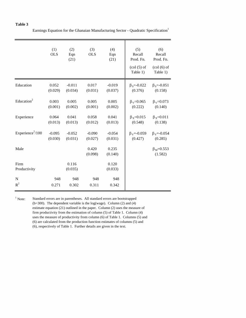
Table 3Earnings Equation for the Ghanaian Manufacturing Sector - Quadratic Specification1
(1) (2) (3) (4) (5) (6)OLS Eqn OLS Eqn Recall Recall
(21) (21) Prod. Fn. Prod. Fn.
(col (5) of (col (6) ofTable 1) Table 1)
Education 0.052 -0.011 0.017 -0.019 βS=-0.022 βS=-0.051(0.029) (0.034) (0.031) (0.037) (0.376) (0.158)
Education2 0.003 0.005 0.005 0.005 βV=0.065 βV=0.073(0.001) (0.002) (0.001) (0.002) (0.222) (0.140)
Experience 0.064 0.041 0.058 0.041 βX=0.015 βX=0.011(0.013) (0.013) (0.012) (0.013) (0.548) (0.138)
Experience2/100 -0.095 -0.052 -0.090 -0.054 βY=-0.059 βY=-0.054(0.030) (0.031) (0.027) (0.031) (0.427) (0.285)
Male 0.420 0.235 βM=0.553(0.098) (0.140) (1.582)
Firm 0.116 0.120Productivity (0.035) (0.033)
N 948 948 948 948R2 0.271 0.302 0.311 0.342
1 Note: Standard errors are in parentheses. All standard errors are bootstrapped (b=300). The dependent variable is the log(wage). Column (2) and (4) estimate equation (21) outlined in the paper. Column (2) uses the measure of firm productivity from the estimation of column (5) of Table 1. Column (4) uses the measure of productivity from column (6) of Table 1. Columns (5) and (6) are calculated from the production function estimates of columns (5) and (6), respectively of Table 1. Further details are given in the text.
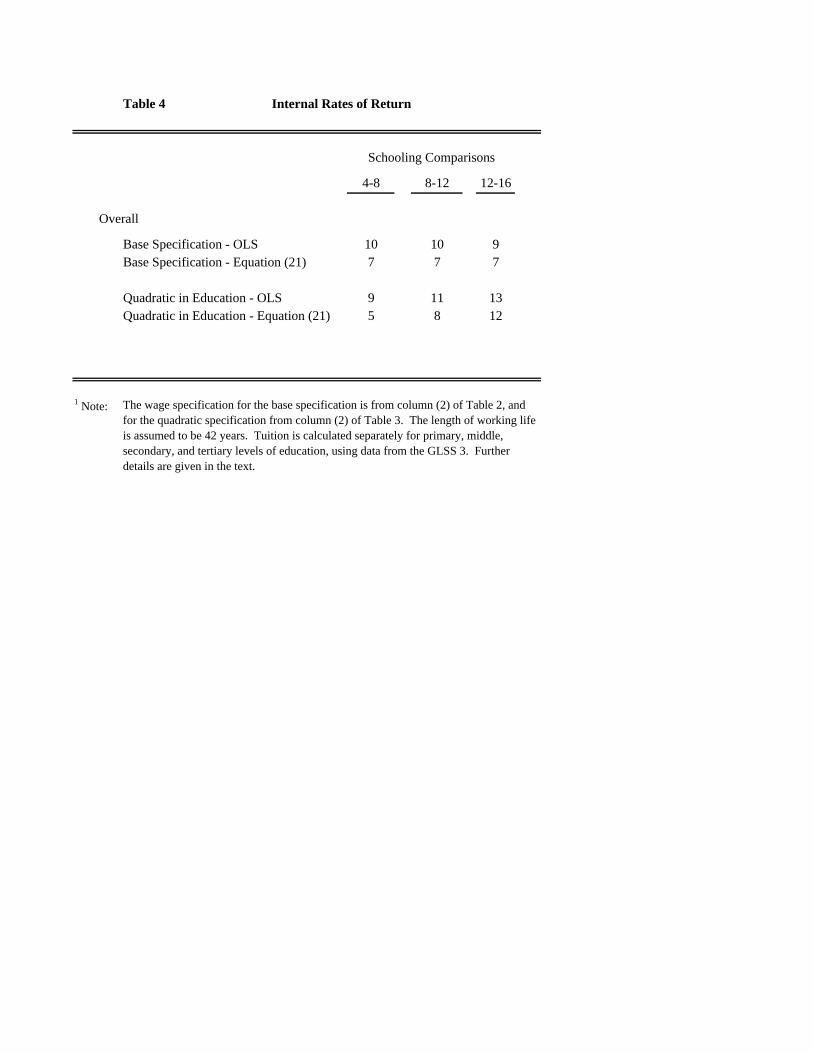
Table 4 Internal Rates of Return
4-8 8-12 12-16
Overall
Base Specification - OLS 10 10 9Base Specification - Equation (21) 7 7 7
Quadratic in Education - OLS 9 11 13Quadratic in Education - Equation (21) 5 8 12
1 Note:
Schooling Comparisons
The wage specification for the base specification is from column (2) of Table 2, and for the quadratic specification from column (2) of Table 3. The length of working life is assumed to be 42 years. Tuition is calculated separately for primary, middle, secondary, and tertiary levels of education, using data from the GLSS 3. Further details are given in the text.

Table 5Earnings Equation for the Ghanaian Manufacturing Sector - Small Firms1
(1) (2) (3) (4) (5) (6) (7) (8) (9) (10) (11) (12)OLS Eqn OLS Eqn OLS Eqn OLS Eqn Prod. Fn. Prod. Fn. Prod. Fn. Prod. Fn.
(21) (21) (21) (21) Parameter Parameter Parameter Parameter
Education 0.112 0.082 0.100 0.080 0.035 -0.044 -0.006 -0.052 βS=0.061 βS=0.065 βS=-0.005 βS=-0.024(0.016) (0.020) (0.015) (0.020) (0.039) (0.046) (0.041) (0.051) (0.111) (0.147) (0.165) (0.332)
Education2 0.005 0.007 0.007 0.008 βV=0.015 βV=0.030(0.002) (0.002) (0.002) (0.002) (0.107) (0.144)
Experience 0.075 0.063 0.069 0.063 0.078 0.066 0.072 0.065 βX=0.040 βX=0.047 βX=0.048 βX=0.044(0.020) (0.023) (0.018) (0.021) (0.019) (0.021) (0.018) (0.020) (0.096) (0.113) (0.079) (0.240)
Exp2/100 -0.113 -0.078 -0.103 -0.078 -0.127 -0.091 -0.119 -0.092 βY=0.021 βY=0.025 βY=0.016 βY=0.011(0.048) (0.058) (0.041) (0.054) (0.047) (0.054) (0.043) (0.052) (0.135) (0.244) (0.131) (0.362)
Male 0.354 0.226 0.430 0.271 βM=-0.015 βM=0.131(0.140) (0.220) (0.139) (0.216) (0.652) (1.582)
Firm 0.210 0.207 0.217 0.217Productivity (0.070) (0.068) (0.065) (0.064)
N 481 481 481 481 481 481 481 481R2 0.280 0.328 0.313 0.362 0.298 0.313 0.343 0.365
1 Note: Standard errors are in parentheses. All standard errors are bootstrapped (b=300). The dependent variable is the log(wage). Column (2), (4), (6), and (8) estimate equation (21) outlined in the paper. The comparable production function parameters for columns (2), (4), (6), and (8) are given in columns (9) through (12), respectively. Further details are given in the text.
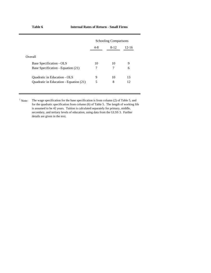
Table 6 Internal Rates of Return - Small Firms
4-8 8-12 12-16
Overall
Base Specification - OLS 10 10 9Base Specification - Equation (21) 7 7 6
Quadratic in Education - OLS 9 10 13Quadratic in Education - Equation (21) 5 8 12
1 Note:
Schooling Comparisons
The wage specification for the base specification is from column (2) of Table 5, and for the quadratic specification from column (6) of Table 5. The length of working life is assumed to be 42 years. Tuition is calculated separately for primary, middle, secondary, and tertiary levels of education, using data from the GLSS 3. Further details are given in the text.
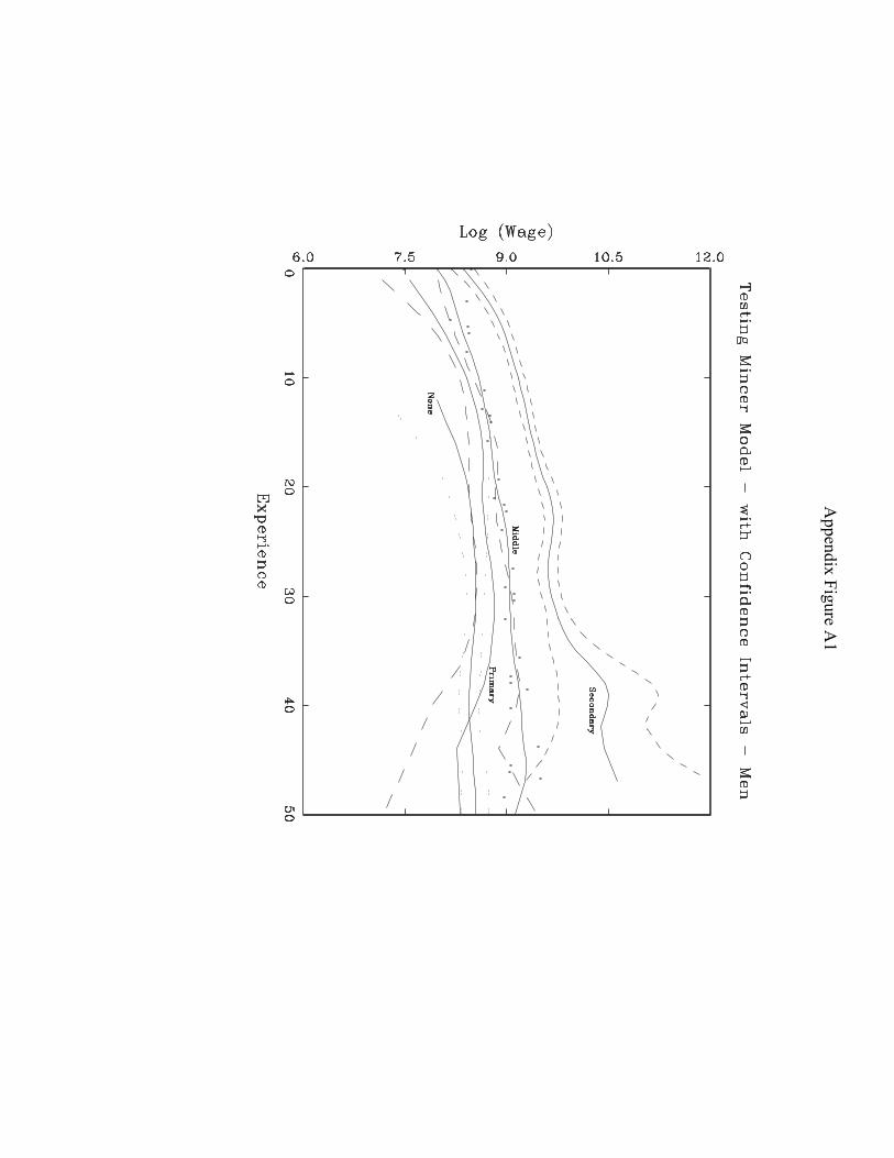
Appendix Figure A
1

Appendix Table A1 Mean Comparison of GMES Sample to GLSS Survey
GLSS SurveyWorker Variables GMES Sample (Employees)
Years of Education 10.6 10.7Years of Experience 20.3 21.9Age 36.8 38.6Hours Worked (Weekly) 46.4 44.8

Appendix Table A2: Tests of Parallelism in Log Earnings Experience Profiles
Estimated Difference in Male Hourly Earnings (cedis) Between Education LevelsExperienceLevel None vs. Primary Primary vs. Middle Middle vs. Secondary
10 2110 1000 470320 315 2741 711630 1813 2442 736740 835 4942 25646
p-value for lines parallel 0.128 0.092 0.290
p-value of joint test that the lines are parallel: .093
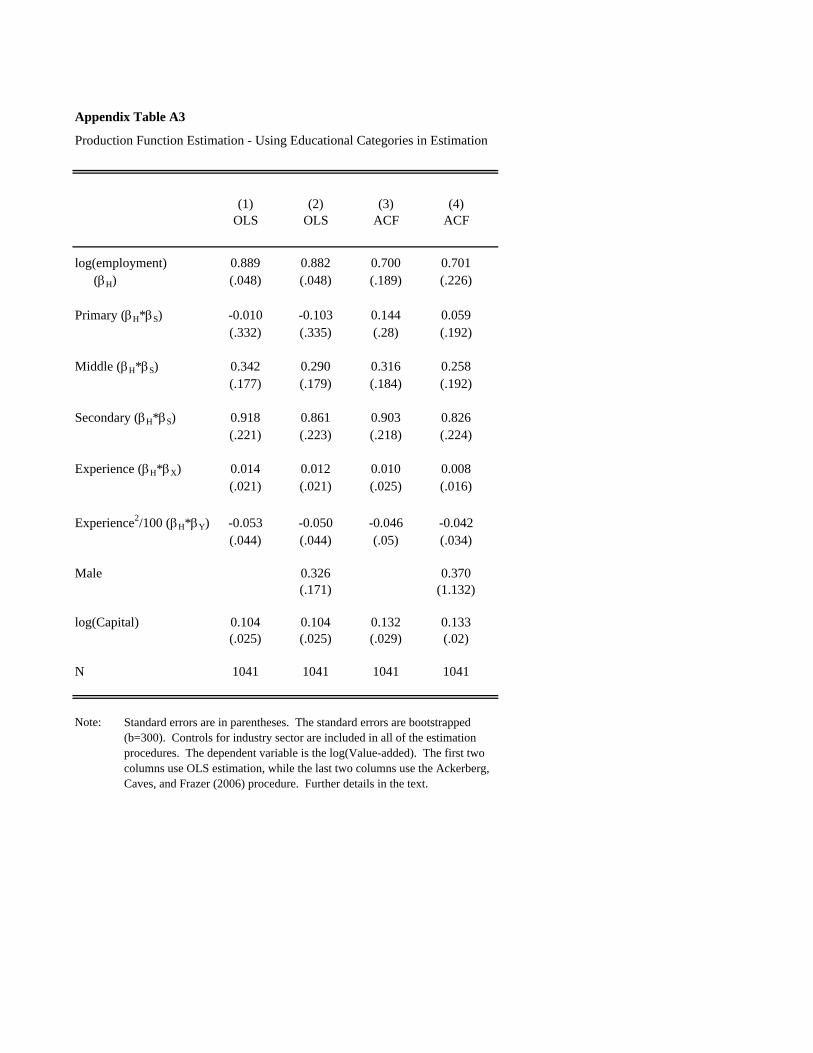
Appendix Table A3
Production Function Estimation - Using Educational Categories in Estimation
(1) (2) (3) (4)OLS OLS ACF ACF
log(employment) 0.889 0.882 0.700 0.701(βH) (.048) (.048) (.189) (.226)
Primary (βH*βS) -0.010 -0.103 0.144 0.059(.332) (.335) (.28) (.192)
Middle (βH*βS) 0.342 0.290 0.316 0.258(.177) (.179) (.184) (.192)
Secondary (βH*βS) 0.918 0.861 0.903 0.826(.221) (.223) (.218) (.224)
Experience (βH*βX) 0.014 0.012 0.010 0.008(.021) (.021) (.025) (.016)
Experience2/100 (βH*βY) -0.053 -0.050 -0.046 -0.042(.044) (.044) (.05) (.034)
Male 0.326 0.370(.171) (1.132)
log(Capital) 0.104 0.104 0.132 0.133(.025) (.025) (.029) (.02)
N 1041 1041 1041 1041
Note: Standard errors are in parentheses. The standard errors are bootstrapped (b=300). Controls for industry sector are included in all of the estimation procedures. The dependent variable is the log(Value-added). The first two columns use OLS estimation, while the last two columns use the Ackerberg, Caves, and Frazer (2006) procedure. Further details in the text.
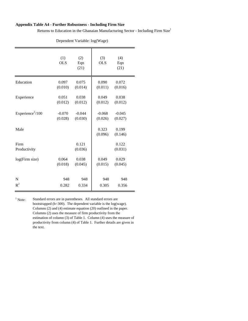
Appendix Table A4 - Further Robustness - Including Firm SizeReturns to Education in the Ghanaian Manufacturing Sector - Including Firm Size1
Dependent Variable: log(Wage)
(1) (2) (3) (4)OLS Eqn OLS Eqn
(21) (21)
Education 0.097 0.075 0.090 0.072(0.010) (0.014) (0.011) (0.016)
Experience 0.051 0.038 0.049 0.038(0.012) (0.012) (0.012) (0.012)
Experience2/100 -0.070 -0.044 -0.068 -0.045(0.028) (0.030) (0.026) (0.027)
Male 0.323 0.199(0.096) (0.146)
Firm 0.121 0.122Productivity (0.036) (0.031)
log(Firm size) 0.064 0.038 0.049 0.029(0.018) (0.045) (0.015) (0.045)
N 948 948 948 948R2 0.282 0.334 0.305 0.356
1 Note: Standard errors are in parentheses. All standard errors are bootstrapped (b=300). The dependent variable is the log(wage). Columns (2) and (4) estimate equation (20) outlined in the paper. Columns (2) uses the measure of firm productivity from the estimation of column (3) of Table 1. Column (4) uses the measure of productivity from column (4) of Table 1. Further details are given in the text.