Embed Size (px)
Citation preview
American Economic Association
Firm Heterogeneity and the Long-run Effects of Dividend Tax ReformAuthor(s): François Gourio and Jianjun MiaoSource: American Economic Journal: Macroeconomics, Vol. 2, No. 1 (January 2010), pp. 131-168Published by: American Economic AssociationStable URL: http://www.jstor.org/stable/25760287 .
Accessed: 10/05/2014 07:32
Your use of the JSTOR archive indicates your acceptance of the Terms & Conditions of Use, available at .http://www.jstor.org/page/info/about/policies/terms.jsp
.JSTOR is a not-for-profit service that helps scholars, researchers, and students discover, use, and build upon a wide range ofcontent in a trusted digital archive. We use information technology and tools to increase productivity and facilitate new formsof scholarship. For more information about JSTOR, please contact [email protected].
.
American Economic Association is collaborating with JSTOR to digitize, preserve and extend access toAmerican Economic Journal: Macroeconomics.
http://www.jstor.org
This content downloaded from 109.175.154.155 on Sat, 10 May 2014 07:32:38 AMAll use subject to JSTOR Terms and Conditions
American Economic Journal: Macroeconomics 2010, 2:1, 131-168
http://www. aeaweb. org/articles.php ?doi=10.1257/mac. 2.1.131
Firm Heterogeneity and the Long-run Effects of Dividend Tax Reform1
By Francois Gourio and Jianjun Miao*
To study the long-run effect of dividend taxation on aggregate capi tal accumulation, we build a dynamic general equilibrium model in which there is a continuum of firms subject to idiosyncratic pro
ductivity shocks. We find that a dividend tax cut raises aggregate
productivity by reducing the frictions in the reallocation of capital across firms. Our baseline model simulations show that when both
dividend and capital gains tax rates are cut from 25 and 20 percent,
respectively, to the same 15 percent level permanently, the aggregate
long-run capital stock increases by about 4 percent. (JEL D21, E22,
E62, G32, G35, H25, H32)
Dividends
are taxed at both the corporate and personal levels in the United States.
This double taxation of dividends may distort investment efficiency. Partly motivated by this consideration, the US Congress enacted the Jobs and Growth Tax
Relief Reconciliation Act (JGTRRA) in 2003. This act reduced the tax rates on dividends and capital gains, and eliminated the wedge between these two tax rates
through 2008. Because one primary goal of JGTRRA is to promote long-run capital formation, these tax cuts could be made permanent. In this paper, we ask the fol
lowing question: What is the quantitative long-run effect of the 2003 dividend tax
reform on aggregate capital accumulation?
This question is of significant interest to economists and policymakers. Economists
disagree about the economic effects of dividend taxation on investment. Two views are prevalent.1 The key consideration is the marginal source of investment finance.
Under the "new view," firms use internal funds to finance investment and do not
*Gourio: Department of Economics, Boston University, 270 Bay State Road, Boston, MA 02215 (e-mail: [email protected]); Miao: Department of Economics, Boston University, 270 Bay State Road, Boston, MA 02215
(e-mail: [email protected]) and Zhongnan University of Economics and Law. We thank John Boyd, Christophe Chamley, Russell Cooper, Dean Corbae, Janice Eberly, Simon Gilchrist, Roger Gordon, Chris House, Bob
King, Narayana Kocherlakota, Anton Korinek, Larry Kotlikoff, Jim Poterba, Joseph Stiglitz, anonymous referees, and seminar participants at Boston University, Chinese University of Hong Kong, the International
Monetary Fund, Northwestern University, the University of Minnesota, the University of Texas at Austin, the
University of Rochester, the 2007 China International Conference in Finance in Chengdu, the 2008 European Econometric Society Meetings, the 2007 Econometric Society Winter and Summer Meetings, the 2007 Midwest Macroeconomics Meeting, and the 2007 Society of Economic Dynamics Meeting for helpful comments.
f To comment on this article in the online discussion forum, or to view additional materials, visit the articles
page at http://www.aeaweb.org/articles.php?doi=10.1257/mac.2.1.131. 1 There is the third "tax irrelevance" view proposed by Merton H. Miller and Myron S. Scholes (1978, 1982).
According to this view, marginal investors do not face differential tax rates on dividends and capital gains. Thus, dividend taxation has no effect on investment. This view has been generally rejected by empirical evidence. See Alan J. Auerbach (2002), Roger Gordon and Martin Dietz (2006), or James M. Poterba and Lawrence H. Summers
(1985) for an exposition of the three views.
131
This content downloaded from 109.175.154.155 on Sat, 10 May 2014 07:32:38 AMAll use subject to JSTOR Terms and Conditions
132 AMERICAN ECONOMIC JOURNAL: MACROECONOMICS JANUARY 2010
raise new equity. Thus, dividend taxation does not influence the user cost of capi tal and investment (Mervyn A. King 1977, Auerbach 1979a, 1979b; and David F. Bradford 1981). Under the "traditional view," the marginal source of funds is new
equity, and the return to investment is used to pay dividends. A dividend tax cut
reduces the user cost of capital and raises investment. Empirical evidence on these two views is inconclusive. For example, Poterba and Summers (1983, 1985) find evidence supporting the traditional view using data from the United Kingdom, and
Mihir A. Desai and Austan D. Goolsbee (2004) find evidence supporting the new view using data from the United States. However, Auerbach and Kevin A. Hassett
(2003) show that in US data, firms behave according to both views, an indication of substantial heterogeneity in the data.
Our paper builds on the existing literature on dividend taxation in two distinct
ways. First, we embed the traditional single-firm model used in empirical studies in a computable dynamic general equilibrium framework.2 Second, we incorporate a
continuum of heterogeneous firms in the model. These firms are subject to idiosyn cratic productivity shocks.3 This firm heterogeneity plays a key role in our analy sis. Specifically, at any point in time, depending on its productivity and its capital stock, a firm finds itself in one of three finance regimes: the equity issuance regime, the dividend distribution regime, or the liquidity constrained regime. In the equity issuance regime, the marginal source of finance is new equity, which reflects the
traditional view of dividend taxation. In the dividend distribution regime, the mar
ginal source of finance is retained earnings, which reflects the new view of dividend
taxation. In the liquidity constrained regime, the firm's investment is limited to the amount of retained earnings. Because of firm heterogeneity, at any point in time
different firms may be in different finance regimes, and respond to the dividend tax cut in different ways.
We show that if there were a representative firm in the economy, dividend taxa
tion would have no effect on long-run capital accumulation, and this highlights the
importance of heterogeneity to our results. A representative firm would, in a deter
ministic steady state, behave according to the new view of dividend taxation, and
would use internal funds rather than equity as its source of financing. We document
empirical evidence that firms' investment and financing patterns are different in
different finance regimes, and that the distribution of firms across different finance
regimes changed following the 2003 tax reform. This evidence supports our model
mechanism.
We use our calibrated model to provide a quantitative evaluation of the long-run effects of the dividend and capital gains tax cuts enacted in 2003.4 We assume that
the benchmark tax system in the initial steady state reflects the federal statutory tax
2 See Auerbach (1979a) for an early overlapping generations model of dividend taxation with a single firm.
See Auerbach and Laurence J. Kotlikoff (1987) for an important comprehensive study of fiscal policy in dynamic
general equilibrium models. See Robert J. Barro (1989) and Marianne Baxter and Robert G. King (1993) for a
general equilibrium analysis of government purchases and the financing of these purchases. 3 In the empirical industrial organization literature, many researchers have found firm level productivity dif
ferences are large and persistent (see Eric J. Bartelsman and Mark Doms 2000 for a survey). 4 The Congressional Budget Office (CBO) uses several models to evaluate JGTRRA. The CBO's (2003) esti
mates are based on an average of model results using two sets of model inputs with one set reflecting the tradi
tional view and the other set reflecting the new view.
This content downloaded from 109.175.154.155 on Sat, 10 May 2014 07:32:38 AMAll use subject to JSTOR Terms and Conditions
VOL. 2 NO. 1 G0URI0 AND MI AO: FIRM LONG-RUN EFFECTS OF DIVIDEND TAX REFORM 133
rates in 2003, before the tax cuts. Because the redistributive effect of the tax cuts is
not our focus of study, we assume that there is a representative household that owns
all firms in the model. In 2003, this household has an average income that falls in
the 25 percent federal income tax bracket. It then faces the 25 percent dividend tax
rate and the 20 percent capital gains tax rate under the 2003 tax system before the
tax cuts.5 In our baseline model, we suppose that the 2003 tax cuts are permanent,
lowering both dividends and capital gains tax rates to the 15 percent level. In this
case, the long-run aggregate capital stock rises by about 4 percent. When we restrict
the tax cut to dividends alone, the effect is much smaller: a permanent reduction
of the dividend tax rate from 25 to 20 percent raises the long-run capital stock by about 0.5 percent. We show that these increases may be smaller when we extend the
baseline model to incorporate a revenue-neutral shift from dividend taxation to labor
income taxation, debt financing, transactions costs of external finance, and share
repurchases. We find that a dividend tax cut has a reallocation effect that generates produc
tivity gains because the dividend tax acts as a friction in the allocation of capital. The intuition is that after a dividend tax cut, some previously liquidity constrained firms move to the equity issuance regime. These firms are more productive, issue new equity, and invest in more capital. Removing the wedge between the tax rate on dividends and the tax rate on capital gains makes the allocation of factors across
firms more efficient.
The general equilibrium price feedback effect is important for our results.
Specifically, the increase in aggregate capital raises the aggregate demand for labor
and, hence, raises the equilibrium wage. The increased wage lowers profits and the returns to investment, and dampens the positive effect of the dividend and capital gains tax cuts. To assess the dampening effect of general equilibrium price move ments quantitatively, we fix the wage rate at its level prior to the tax cuts, and show that the increase in aggregate capital after the tax cuts in partial equilibrium could be six times larger than that in general equilibrium.
Our paper is related to a vast literature on investment and dividend taxation in
public finance, corporate finance, and macroeconomics. To our knowledge, our
paper provides the first computable dynamic general equilibrium model with firm
heterogeneity to evaluate the 2003 dividend tax cut. We show both heterogeneity and general equilibrium price movements are critical to a proper quantitative assess ment of this issue. Our model framework is related to Joao F. Gomes (2001), who
analyzes the issue of investment-cash flow sensitivity,6 although, in contrast to our
work, he does not address taxation or tax policy. We extend his model to incorporate personal and corporate taxation, and adjustment costs. While both models feature three finance regimes, the three finance regimes in our model are generated through
5 Although dividend taxes are skewed toward upper income households, our calibrated 25 percent tax rate
is not too low since a large share of equity is held by low-tax institutional investors, such as pension funds (see Poterba 2004). 6
There is a large empirical literature on the investment-cash flow sensitivity (e.g., Steven M. Fazzari, Robert Glenn Hubbard, and Bruce C. Petersen 1988; Simon Gilchrist and Charles Himmelberg 1995; Russell Cooper and Joao Ejarque 2003; Nathalie Moyen 2004; and Christopher A. Hennessy and Toni M. Whited 2007). This literature argues that external finance is costly because of taxes, asymmetric information, and transactions costs.
This content downloaded from 109.175.154.155 on Sat, 10 May 2014 07:32:38 AMAll use subject to JSTOR Terms and Conditions
134 AMERICAN ECONOMIC JOURNAL: MACROECONOMICS JANUARY 2010
differential tax treatments on dividends and capital gains, as opposed to transaction costs of external financing modeled in Gomes (2001).
Our paper is also related to Christopher L. House and Matthew D. Shapiro (2006), who analyze the quantitative effects of the timing of the tax rate changes enacted in 2001 and 2003. Unlike our paper, they assume a representative firm in the model and do not consider the question we analyzed here. Anton Korinek and Joseph E. Stiglitz
(2009) provide a partial equilibrium model to study the effects of dividend taxation on investment. They show that firm heterogeneity implies that a dividend tax cut
has a small effect on aggregate investment. Unlike our model, their model lacks the
general equilibrium mechanism.
The remainder of the paper is organized as follows. Section I documents evidence on the changes in corporate behavior after the 2003 dividend tax cut. Section II sets
up the model. Section III analyzes a single firm's decision problem, and the effects of dividend taxation in partial equilibrium. Section IV provides quantitative results.
Section V considers several extensions. Section VI concludes. Technical details
regarding model solution and data construction are relegated to the Appendix.
I. Empirical Evidence on Corporate Behavior from the 2003 Dividend Tax Cut
The 2003 JGTRRA makes two major changes in tax law. First, the capital gains tax rate is reduced from the previous 20 percent for individuals in the top 4 tax
brackets (facing marginal tax rates of 25, 28, 33, and 35 percent) to 15 percent. It
is reduced from the previous 10 percent for individuals in the lower 2 tax brackets
(facing marginal tax rates of 10 and 15 percent) to 5 percent. Second, dividends are
taxed at the same rate as capital gains. In particular, dividends are taxed at the rate of
15 percent for individuals in the top 4 tax brackets. Dividends were previously taxed as regular income. In this section, we document empirical evidence on the effects
of the 2003 dividend tax cut on corporate investment and financing behavior. This
evidence complements the findings of Raj Chetty and Emmanuel Saez (2005). Our
data are drawn from the COMPUSTAT database. Appendix Section A describes the
construction of our data in detail.
We sort firms according to their finance regimes: firms distributing dividends
(dividend distribution regime), firms issuing new equity but not paying dividends
(equity issuance regime), and firms neither issuing new equity nor paying dividends
(liquidity constrained regime). Because many firms in our data issue very small
amounts of equity, we say that a firm issues new equity if the ratio of equity issu
ance to the capital stock is greater than or equal to 2 percent.7 We find that about
20 percent of firms in our data in any given year distribute dividends and issue new
equity. This behavior is puzzling for the standard theory based on taxes, since it
implies that there exists a profitable opportunity to reduce dividends and equity issu ance. As Stephen Bond and Costas Meghir (1994) argue, the observed behavior may be explained by transactions costs or signaling theory (e.g., Sudipto Bhattacharya
7 Changing this threshold to 1 percent does not affect our results significantly.
This content downloaded from 109.175.154.155 on Sat, 10 May 2014 07:32:38 AMAll use subject to JSTOR Terms and Conditions
VOL. 2 NO. 1 GOURIO AND MIAO: FIRM LONG-RUN EFFECTS OF DIVIDEND TAX REFORM 135
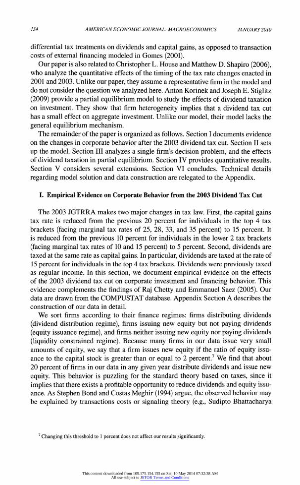
Table 1?Distribution of Firms across Finance Regimes in the Data (Average over 1988-2002)
Share of firms Share of capital Share of investment
Earnings-capital ratio
Investment-capital ratio Tobin's q
Equity issuance regime
0.230 0.028 0.039 0.567 0.290 3.768
Liquidity constrained regime
0.297 0.059 0.057 0.275 0.193 1.784
Dividend distribution regime
0.474 0.913 0.904 0.355 0.194 2.837
Notes: The share of firms for a regime is equal to the total number of firms in that regime divided by the total num ber of firms in all regimes. The share of capital (investment) for a regime is equal to the total capital stock (invest ment) of the firms in that regime divided by aggregate capital stock (investment) of all firms. The earnings-capital ratio for a regime is equal to the earnings of the firms in that regime divided by their total capital stock, i.e., it is
capital-weighted. The investment-capital ratio and Tobin's q are computed in a similar way.
1979). Since the objective of our study is not on the preceding "dividend puzzle," we
group these firms into the dividend distribution regime. We compute the investment-to-capital ratio in any year for firms in each finance
regime as their total investment in that year divided by their total capital in that year.
Similarly, we compute ratios of earnings to capital and Tobin's q in a year for firms in each finance regime. Table 1 presents the average across years from 1988 to 2002, before the dividend tax cut.
Table 1 reveals that, on average, about half of the firms pay dividends. The rest is divided into two approximately equal-sized groups: firms that issue equity, and firms that do not. Consistent with the existing literature (e.g., Tim Loughran and Jay R. Ritter 1997; Evgeny Lyandres, Le Sun, and Lu Zhang 2008), this table shows that firms issuing equity are significantly more productive than the rest, as measured by the earnings-to-capital ratio. These firms are small (measured by capital) and have
high Tobin's q. Apparently, these "growth firms" are productive, have good invest ment opportunities, and require external finance to make investments. The two other
groups have similar investments, but the firms paying dividends have higher Tobin's
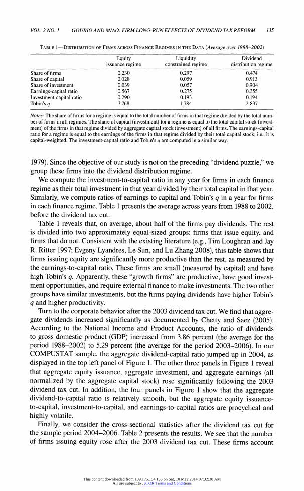
q and higher productivity. Turn to the corporate behavior after the 2003 dividend tax cut. We find that aggre
gate dividends increased significantly as documented by Chetty and Saez (2005). According to the National Income and Product Accounts, the ratio of dividends to gross domestic product (GDP) increased from 3.86 percent (the average for the
period 1988-2002) to 5.29 percent (the average for the period 2003-2006). In our COMPUSTAT sample, the aggregate dividend-capital ratio jumped up in 2004, as
displayed in the top left panel of Figure 1. The other three panels in Figure 1 reveal that aggregate equity issuance, aggregate investment, and aggregate earnings (all normalized by the aggregate capital stock) rose significantly following the 2003 dividend tax cut. In addition, the four panels in Figure 1 show that the aggregate dividend-to-capital ratio is relatively smooth, but the aggregate equity issuance
to-capital, investment-to-capital, and earnings-to-capital ratios are procyclical and
highly volatile.
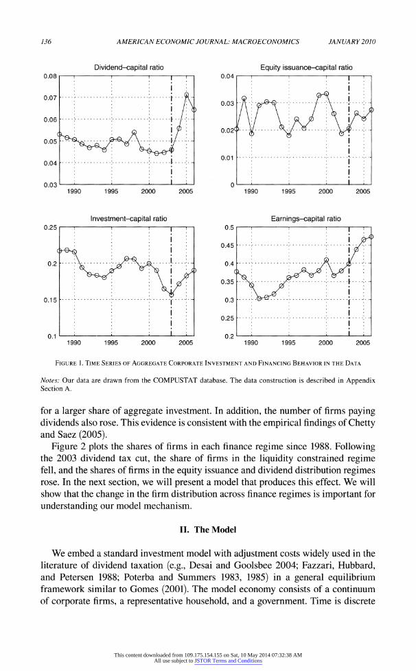
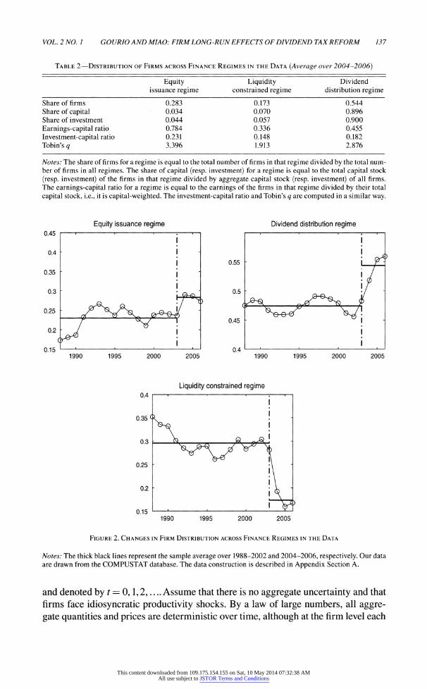
Finally, we consider the cross-sectional statistics after the dividend tax cut for the sample period 2004-2006. Table 2 presents the results. We see that the number of firms issuing equity rose after the 2003 dividend tax cut. These firms account
This content downloaded from 109.175.154.155 on Sat, 10 May 2014 07:32:38 AMAll use subject to JSTOR Terms and Conditions
136 AMERICAN ECONOMIC JOURNAL: MACROECONOMICS JANUARY 2010
Investment-capital ratio Earnings-capital ratio
1990 1995 2000 2005 1990 1995 2000 2005
Figure 1. Time Series of Aggregate Corporate Investment and Financing Behavior in the Data
Notes: Our data are drawn from the COMPUSTAT database. The data construction is described in Appendix Section A.
for a larger share of aggregate investment. In addition, the number of firms paying dividends also rose. This evidence is consistent with the empirical findings of Chetty and Saez (2005).
Figure 2 plots the shares of firms in each finance regime since 1988. Following the 2003 dividend tax cut, the share of firms in the liquidity constrained regime fell, and the shares of firms in the equity issuance and dividend distribution regimes rose. In the next section, we will present a model that produces this effect. We will
show that the change in the firm distribution across finance regimes is important for
understanding our model mechanism.
II. The Model
We embed a standard investment model with adjustment costs widely used in the
literature of dividend taxation (e.g., Desai and Goolsbee 2004; Fazzari, Hubbard, and Petersen 1988; Poterba and Summers 1983, 1985) in a general equilibrium framework similar to Gomes (2001). The model economy consists of a continuum
of corporate firms, a representative household, and a government. Time is discrete
This content downloaded from 109.175.154.155 on Sat, 10 May 2014 07:32:38 AMAll use subject to JSTOR Terms and Conditions
VOL. 2 NO. 1 GOURIO AND MI AO: FIRM LONG-RUN EFFECTS OF DIVIDEND TAX REFORM 137
Table 2?Distribution of Firms across Finance Regimes in the Data (Average over 2004-2006)
Equity issuance regime
Liquidity constrained regime
Dividend distribution regime
Share of firms Share of capital Share of investment
Earnings-capital ratio
Investment-capital ratio Tobin's q
0.283 0.034 0.044 0.784 0.231 3.396
0.173 0.070 0.057 0.336 0.148 1.913
0.544 0.896 0.900 0.455 0.182 2.876
Notes: The share of firms for a regime is equal to the total number of firms in that regime divided by the total num ber of firms in all regimes. The share of capital (resp. investment) for a regime is equal to the total capital stock
(resp. investment) of the firms in that regime divided by aggregate capital stock (resp. investment) of all firms. The earnings-capital ratio for a regime is equal to the earnings of the firms in that regime divided by their total
capital stock, i.e., it is capital-weighted. The investment-capital ratio and Tobin's q are computed in a similar way.
Equity issuance regime Dividend distribution regime
0.55
0.5
1990 1995 2000 2005
0.45
0.4
*****
1990 1995 2000 2005
Liquidity constrained regime 0.4
0.35
0.3
0.25
0.2
0.15 1990 1995 2000 2005
Figure 2. Changes in Firm Distribution across Finance Regimes in the Data
Notes: The thick black lines represent the sample average over 1988-2002 and 2004-2006, respectively. Our data are drawn from the COMPUSTAT database. The data construction is described in Appendix Section A.
and denoted by t ? 0,1,2,.... Assume that there is no aggregate uncertainty and that
firms face idiosyncratic productivity shocks. By a law of large numbers, all aggre
gate quantities and prices are deterministic over time, although at the firm level each
This content downloaded from 109.175.154.155 on Sat, 10 May 2014 07:32:38 AMAll use subject to JSTOR Terms and Conditions
138 AMERICAN ECONOMIC JOURNAL: MACROECONOMICS JANUARY 2010
firm still faces idiosyncratic uncertainty. We will focus on steady-state stationary equilibrium in which all aggregate variables are constant over time.
We begin by describing the firms' decision problem. Firms are ex ante iden
tical, and are subject to idiosyncratic productivity shocks. They differ ex post in that they may experience different histories of productivity shocks. Assume that these shocks are generated by a Markov process with transition function given by
Q:Zx 2->[0,l], where (Z,Z) is a measurable space. In order to focus on the key issue of dividend taxation in the simplest possible way,
we make two assumptions. First, as in most papers in the literature, we consider flat taxes with full loss offset provisions. In particular, we assume that firms face corpo rate income tax at the constant rate rc, while individuals face constant tax rates rd on
dividends, rt on labor and interest income, and rg on accrued capital gains.8 Second, we abstract from debt and assume that firms are all equity financed, as in Auerbach and Hassett (2002), Desai and Goolsbee (2004), and Poterba and Summers (1985). Incorporating debt financing would complicate our analysis since we would need to
include debt as an additional state variable in the dynamic programming problem
(8). A simple way to incorporate debt financing is to assume that a fixed fraction of
capital is financed by debt, as in Poterba and Summers (1983). We will consider this extension in Section VB.
Because all firms are ex ante identical, we consider a single firm's decision prob lem, and then study aggregation. In order to formulate this problem, we first derive the firm's equity valuation equation. Let the ex-dividend equity value be Pt at date t.
In equilibrium, the following no arbitrage equation must hold:
where Et[-\ denotes the expectation operator conditional on the firm's history of
idiosyncratic shocks, Rt denotes the required return to equity, dM is the firm's divi
dend payment, and Pf+l is the period t + 1 value of equity outstanding in period t.
The firm may issue new shares or repurchase old shares. Thus, equity value at date
t + 1 satisfies Pt+l = + st+h where sM denotes the value of new shares issued
(repurchased) if st+x > (<) 0. Many researchers argue that external equity financing is costly due to asymmetric information or transactions costs. In the baseline model
here, we do not consider such costly external financing. Instead, we consider this
issue in Section VC.
We will show that since there is no aggregate uncertainty, the steady-state equi librium required return to equity satisfies:
A. Firms
(i) R, = ? Et[(l -
rd) dt+l + (1 -
rg)(P;?+1 -
/>,)],
(2) R,= (\-T^r,
8 In the United States, capital gains are taxed on realization rather than on accrual. Incorporating a realiza tion-based capital gains tax would complicate our analysis significantly, and it is not important in this context.
This content downloaded from 109.175.154.155 on Sat, 10 May 2014 07:32:38 AMAll use subject to JSTOR Terms and Conditions
VOL. 2 NO. 1 GOURIO AND MIAO: FIRM LONG-RUN EFFECTS OF DIVIDEND TAX REFORM 139
where r is the steady-state equilibrium interest rate. Using equations (1) and (2), we can derive
(3) P,[(l -
T,-)r + 1 - rj =
Et[{\ -
rd)dt+l + (1 -
rg)(Pt+1 -
st+l)}.
We define the cum-dividend equity value Vt+l as
(4) = " + J?f~ dt+i.
Using (3), we can then show that
r*\ 1/ 1 " Td a , EtlVt+l] (5) V' =
T=V*-*+ l+rfl-Tj/fl-rJ
We will use this equation to formulate the firm's dynamic programming problem. The firm combines labor and capital to produce output. Suppose the firm has a
decreasing-returns-to-scale production function given by F(k9 /; z), where k, /, and
z denote capital, labor, and productivity shock, respectively. Assume that F( ) is
strictly increasing, strictly concave, and satisfies the usual Inada conditions. We can
then derive the operating profit function 7r(?,z;w) by solving the following static labor choice problem:
(6) 7c(k,z; w) = max {F(k, /;z)
- wl},
where w denotes the wage. This problem gives the labor demand /(&, z; w) and the
output supply y(k, z\ w) ?
F(k, 1{K z\ w); z). The firm can also make investments x to increase its capital stock so that the capi
tal stock in the next period k' satisfies:
(7) k' = (1 -
S)k + x,
where 6 G (0,1) denotes the depreciation rate. Investments incur adjustment costs.
For simplicity, we consider the quadratic adjustment cost function, ipx2/(2k), widely used in the empirical investment literature (e.g., Cooper and John C. Haltiwanger 2006). The firm's problem is then to choose investment and financial policies so as
to maximize its equity value.
Let V(k,z;w) denote equity value at the state (k,z) given that the equilibrium steady-state wage rate is w. Then by (5), V(k,z',w) satisfies the following Bellman
equation:
(8) V(k,Z;W) = - , + { + ̂ _ ^
_ / V(kW,W) Q{zM\
This content downloaded from 109.175.154.155 on Sat, 10 May 2014 07:32:38 AMAll use subject to JSTOR Terms and Conditions
140 AMERICAN ECONOMIC JOURNAL: MACROECONOMICS JANUARY 2010
subject to (7) and
(9) x + ipx2 + d = (1
- rc) 7r (k,z\w) + rcSk + s, 2k
(10) d>0,
(11) s>0.
Equation (9) describes the flow of funds condition for the firm. The source of funds consists of after-tax profits, depreciation allowances, and new equity issuance. The use of funds consists of investment expenditure, adjustment costs, and dividend pay ments.9 Dividend payments cannot be negative. We impose constraint (10). There
may be further constraints on dividend payments. For example, one may assume that
the firm should pay a fraction of earnings as dividends (e.g., Auerbach 2002; Poterba
and Summers 1983). The motivation for a constraint like this typically comes from
asymmetric information problems or agency problems between managers and share
holders, and lies outside the purpose of our present investigation. While share repurchases are allowed in the United States, there are several rea
sons to think that share repurchases are either effectively constrained or costly.
Regular share repurchases may lead the Internal Revenue Service (IRS) to treat the
repurchases as dividends, thus erasing their tax advantage. Additional repurchase costs may arise as a result of asymmetric information (see, e.g., Michael J. Brennan
and Anjan V. Thakor 1990 and Michael J. Barclay and Clifford W. Smith, Jr. 1988). For simplicity, we follow most papers in the literature to impose constraint (ll).10 Because we rule out share repurchases, the baseline model cannot address the "divi
dend puzzle" which asks why firms pay dividends given the tax advantage of share
repurchases. In Section VD, we will relax this assumption and follow Poterba and
Summers (1985) to impose a constraint that share repurchases are bounded by some
maximal amount. We refer the reader to Gordon and Dietz (2006) for a survey of
models of the dividend puzzle.
By a standard dynamic programming argument (see Hennessy and Whited 2005
or Nancy L. Stokey, and Robert E. Lucas, Jr., and Edward C. Prescott 1989), one
can show that there is a unique value function V satisfying the Bellman equation (8). Also V is continuous, strictly increasing, and strictly concave in k. Thus, there exist
unique decision rules denoted by
(12) x = x (k, z\ w),k' = g(k9 z;w),s = s (k, z\ w)9d = d (?, z\ w).
9 Note that we treat the adjustment cost as part of investment expenditures so that it is not tax deductible. One
may treat the adjustment cost as part of a wage bill so that it is tax deductible. This alternative modeling does not
change our key insights. 10 See, for example, Auerbach (1979b, 2002), Gomes (2001), Bond and Meghir (1994), Desai and Goolsbee
(2004), and Hennessy and Whited (2005).
This content downloaded from 109.175.154.155 on Sat, 10 May 2014 07:32:38 AMAll use subject to JSTOR Terms and Conditions
VOL. 2 NO. 1 GOURIO AND MIAO: FIRM LONG-RUN EFFECTS OF DIVIDEND TAX REFORM 141
B. Stationary Distribution and Aggregation
Because there is a continuum of firms that are subject to idiosyncratic shocks, there is a cross-sectional distribution \i of firms over the state (k,z). By Stokey, Lucas, and Prescott (1989), the law of motion for the firm distribution is given by
(13) //(A x B) = J lg{U;w) eA Q(z,B) n (dk,dz),
where 1 is an indicator function, and A and B are Borel sets. Note that we suppress the dependence of distributions on the wage w. When //
= \i = //*, we call /i* the
stationary distribution. Given the stationary distribution //, we can compute the fol
lowing aggregate quantities:
aggregate output supply,
(14) F(/i*;w) = |y(k,z\w) fi*(dk,dz);
aggregate labor demand,
(15) Ld(fjL*'9w) = j l(k9z;w) ii\dk,dz)\
aggregate investment,
(16) /(/i*;w) = jx(k,z',w) fi(dk,dz)\ and
aggregate adjustment cost,
(17) ?(^ =
C. Household
The representative household derives utility from consumption and leisure accord
ing to the standard time-additive utility function:
(18) OO
E l3'U(Ct,Q, t=0
This content downloaded from 109.175.154.155 on Sat, 10 May 2014 07:32:38 AMAll use subject to JSTOR Terms and Conditions
142 AMERICAN ECONOMIC JOURNAL: MACROECONOMICS JANUARY 2010
where (3 is the discount factor; Ct denotes consumption; Lt denotes labor supply; and U satisfies Ux > 0, Uxx < 0, U2 < 0, U22 < 0, and the Inada conditions. The house hold owns all firms and trades firms' shares. In addition, the household also trades a
risk-free bond in zero net supply. It pays dividend taxes, personal income taxes, and
capital gains taxes.11 Thus, the budget constraint is given by
(19) Ct+ \pt9t+xdpt + bM
= j[(l~
rd) dt + P?- rg(PQt -
Pt_x)) Otdnt + (1 + (1 -
r?r
+ (l-7>fL,+ r,,
where 9t denotes the shares owned by the household, bt denotes bond holdings, rt denotes the interest rate, and Tt denotes the transfer from the government. In equi librium, 9t
? 1 and bt = 0.
The household's problem is to choose consumption, labor supply, and trading
strategies to maximize its utility (18) subject to (19). We consider the household problem in a stationary equilibrium in which the interest rate rt, the wage rate wt, and aggregate quantities are constant over time. As in Gomes (2001), one can show that in a stationary equilibrium the intertemporal marginal rate of substitution (the pricing kernel) is equal to (5. Thus, the interest rate satisfies:
(20) 0(r(l -
r,.) + 1) = 1,
and the required return to equity is given by (2). In addition, in the steady state, the household's problem can be simplified to the following static problem:
(21) max U(C,L)
subject to
(22) C = (1 -
rd) Jd{k,z;w)ti(dk,dz) -
(1 -
rg) js{k,z\^)n*{dk,dz)
+ (1 -T>L + r(w,//),
11 According to the US tax system, capital losses are tax deductible within some limit. For tractability, we
ignore this limit in our model.
This content downloaded from 109.175.154.155 on Sat, 10 May 2014 07:32:38 AMAll use subject to JSTOR Terms and Conditions
VOL. 2 NO. 1 GOURIO AND MI AO: FIRM LONG-RUN EFFECTS OF DIVIDEND TAX REFORM 143
where T(w,f/,*) is the steady-state transfer. This problem gives decision rules for
consumption C(h>, //, T(w9 //*)) and labor supply Ls(w, //, T(w9 fx*)).
Because the focus of the paper is on the distortionary effect of dividend taxation
on investment, we assume that tax revenues collected by the government are rebated
to the household in a lump-sum manner. Thus, we abstract from other distortionary effects associated with using distortionary taxation to finance government spending on goods and services. Incorporating government spending would complicate our
analysis since a tax cut must eventually be financed with some combination of other
tax increases or spending cuts. We also do not consider government debt. The analy sis of how the dividend and capital gains tax cut is financed is beyond the scope of
the present paper and is left for future research. In Section VA, we extend our model
to allow for revenue-neutral tax reform by shifting from dividend taxation to labor
income taxation.
Because the government collects corporate income taxes, dividend taxes, per sonal income taxes, and capital gains taxes, and transfers these tax revenues to the
household, the government budget constraint is given by:
A stationary equilibrium consists of a constant wage rate w, a stationary distribu
tion of firms //, aggregate quantities, C(/i*; w), /(//*; w), *J/(^*; w), Y(/j,*;w), Z/(//; w), Z/(//;w), and decision rules, k' ? g(k,z',w), x = x(k,z\w), s = s{k,z\w), d = d(k, z\ w), such that the decision rules solve the firm's problem (8); C(w,/i*, T(w, //)) and Z/(w,//, T(w9 //*)) solve the problem by (21); /i* satisfies equation (13) and aggre gate quantities satisfy equations (14)?(17); T(w,/jl*) satisfies the government budget constraint (23); and markets clear,
D. Government
(23) T ? rc fa (k>z;w) -
5k) fi(dk,dz) + rd \d(k9z;w) \i (dk9dz)
E. Stationary Equilibrium
(24) 4? = %';4
(25)
III. Analysis of a Single Firm's Decision Problem
In order to analyze the general equilibrium effects of a dividend tax cut, we first
analyze a single firm's decision problem in partial equilibrium. We fix the wage rate and suppress the variable w throughout this section.
This content downloaded from 109.175.154.155 on Sat, 10 May 2014 07:32:38 AMAll use subject to JSTOR Terms and Conditions
144 AMERICAN ECONOMIC JOURNAL: MACROECONOMICS JANUARY 2010
It proves more convenient to rewrite the dynamic programming problem (8) as
the following sequence problem:
(26) max E xt, kt+l,st
1
lS o~+7(i -rm -rg)y vi dt~st
subject to
(27)
(28)
(29)
(30)
X, + + d, = (l- Tc) 7T (k?zt) + TcSk, + st,
kt+l = (1-5)^ + x?
d,>0,
st>0.
Let qt, A? > 0 and A? > 0 be the Lagrange multipliers associated with the constraints
(28)-(30), respectively. As is well known, q, can be interpreted as the shadow price of capital and is referred to as the marginal q. Using equation (27) to eliminate d? we obtain the following first-order conditions:
(31) st:\^-+Xdt+\st=h
(32) x,:qt = [T-^+\U J [l
+ ^ l-rg+X^){l+ k
(33) kt+1 : q, = i + ̂ _ ^
_ ^
Et {qt+1
(1-5) +
We also have the usual transversality condition and the complementary slackness
condition, which are omitted here for simplicity.
A. Financial Policy
We start by analyzing the firm's financial policy, holding the investment policy fixed. This financial policy is determined by equation (31), which has the following interpretation. Raising one unit of new equity to pay dividends relaxes the dividend
constraint and the share repurchase constraint. In addition, the shareholder receives
This content downloaded from 109.175.154.155 on Sat, 10 May 2014 07:32:38 AMAll use subject to JSTOR Terms and Conditions
VOL. 2 NO. 1 G0URI0 AND MIAO: FIRM LONG-RUN EFFECTS OF DIVIDEND TAX REFORM 145
(1 ?
Tj)/(1 ?
rg) units of after tax dividends. Thus, the expression on the left-hand side of (31) represents the marginal benefit to the shareholder. On the other hand, one unit increase in new shares lowers equity value by one unit, and the expression on the right-hand side of (31) gives the marginal cost to the shareholder. Equation (31) requires that the preceding marginal benefit and marginal cost must be equal at optimum.
If rd = Tg, then there is no tax differential between dividends and retained earn
ings. Equation (31) implies that Xdt =
Xst = 0. In this case, the firm's financial policy
is irrelevant. That is, it does not matter for firm value and investment policy how much earnings to retain for use as internal finance, rather than distributing dividends and raising new equity in the external equity market. More formally, in the firm's
problem (26), the payout dt -
st can be determined. However, dividends dt and new
equity st are indeterminate. This is the celebrated Miller and Franco Modigliani (1961) dividend policy irrelevance theorem.
However, if rd ̂ rg, then the firm's financial policy matters. Before the 2003 dividend tax cut, the tax rate on dividends in the United States was higher than the tax rate on capital gains, so we assume that rd > rg. In this case, it follows from (31) that we cannot have A?
= \st
= 0. That is, it is not optimal for the firm to simultane
ously issue new equity and distribute dividends. The intuition is simple. New equity or share repurchases change equity value and, hence, capital gains. Thus, they are taxed at the capital gains rate rg. By contrast, dividends are taxed at a higher rate rd. To maximize equity value, the firm should reduce dividends, but repurchase shares to the extent possible. This implies that one of the constraints (10) and (11) must be binding. This observation gives us three cases to consider. Each case corresponds to a different finance regime (see Hennessy and Whited 2005, and Stiglitz 1973).
In the first case, dt > 0 and st = 0. We call this case the dividend distribution
regime. In this regime, the firm has enough retained earnings to finance invest ment and to distribute dividends. In addition, the firm has exhausted opportunities to
repurchase shares so that the share repurchase constraint binds, st ? 0. This regime
corresponds to the "new view" of dividend taxation. In the second case, dt ? 0 and
st > 0. We call this case the equity issuance regime. In this regime, the firm does not have enough internal funds to distribute dividends. Instead, the firm reduces dividends to the extent possible, so that the nonnegative dividend constraint binds, dt
= 0. In addition, the firm has unused opportunities to repurchase shares in that
st > 0. The marginal source of investment finance is the external equity market. This
regime reflects the traditional view of divided taxation. In the third case, dt = 0 and
st ? 0. We call this case the liquidity constrained regime. In this regime, the firm
exhausts all internal funds to finance investment and, hence, does not distribute divi dends. In addition, the firm does not issue new equity because the marginal return to investment does not justify the reduction in equity value due to share dilution. In this regime, a windfall addition to current earnings, which conveys no information about the firm's future profitably, will raise investment. The presence of firms in this
regime may account for the excess sensitivity of investment to measures of internal funds.
We should emphasize that finance regimes may change over time because of the stochastic productivity shocks and the intertemporal investment policy. As will be
This content downloaded from 109.175.154.155 on Sat, 10 May 2014 07:32:38 AMAll use subject to JSTOR Terms and Conditions
146 AMERICAN ECONOMIC JOURNAL: MACROECONOMICS JANUARY 2010
discussed later, this implies that we cannot simply do comparative statics based on
the current source of marginal finance. In addition, in the cross section with firm
heterogeneity, different firms may be in different finance regimes. Next, we turn to
the firm's investment policy.
B. Investment Policy
We first derive a ^-theoretic investment equation, and then derive the user cost
of capital. Based on this derivation, we analyze the effect of dividend taxation on
investment in partial equilibrium. This analysis generalizes Auerbach (1979b), J. S. S. Edwards and M. J. Keen (1984), and Poterba and Summers (1985) to include
adjustment costs.
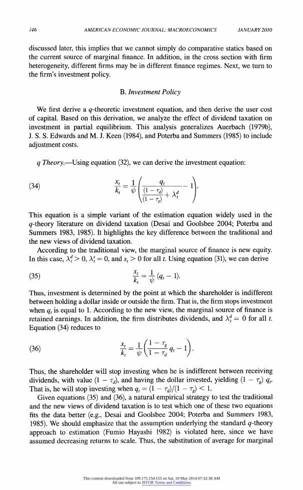
q Theory.?Using equation (32), we can derive the investment equation:
(34) ? = -1)
This equation is a simple variant of the estimation equation widely used in the
^-theory literature on dividend taxation (Desai and Goolsbee 2004; Poterba and
Summers 1983, 1985). It highlights the key difference between the traditional and the new views of dividend taxation.
According to the traditional view, the marginal source of finance is new equity. In this case, Af > 0, AJ = 0, and st > 0 for all t. Using equation (31), we can derive
(35) t = i(*-1)
Thus, investment is determined by the point at which the shareholder is indifferent
between holding a dollar inside or outside the firm. That is, the firm stops investment
when qt is equal to 1. According to the new view, the marginal source of finance is
retained earnings. In addition, the firm distributes dividends, and Af = 0 for all t.
Equation (34) reduces to
Thus, the shareholder will stop investing when he is indifferent between receiving
dividends, with value (1 -
rd), and having the dollar invested, yielding (1 -
rg) qt. That is, he will stop investing when qt = (1
- rd)/(l
? rg) < 1.
Given equations (35) and (36), a natural empirical strategy to test the traditional
and the new views of dividend taxation is to test which one of these two equations fits the data better (e.g., Desai and Goolsbee 2004; Poterba and Summers 1983,
1985). We should emphasize that the assumption underlying the standard ^-theory
approach to estimation (Fumio Hayashi 1982) is violated here, since we have assumed decreasing returns to scale. Thus, the substitution of average for marginal
This content downloaded from 109.175.154.155 on Sat, 10 May 2014 07:32:38 AMAll use subject to JSTOR Terms and Conditions
VOL. 2 NO. 1 GOURIO AND MI AO: FIRM LONG-RUN EFFECTS OF DIVIDEND TAX REFORM 147
q produces a measurement error (see Gomes 2001). As Cooper and Ejarque (2003) point out, this misspecification of g-theory based models implies that any inferences
about the size of the quadratic adjustment cost, or the significance about the financial
variable, may be invalid.
What seems counterintuitive is that under the traditional view, tax parameters do
not enter (35), but they appear in (36). In fact, the intuition is easy to explain. Solving equation (33) recursively forward, and using the law of iterated expectation and the
transversality condition, we obtain
(37)
where
(38)
qt = Et (1
- gy-1 mpkt +j
Jt(i + r(i-Ti.)/(i-Tg)y j
mpkt+j = + [(!
- Tc) ""i (kt+j'Zt+j) + Tc6 + ^x /(2*?J
This equation simply says that marginal q reflects the firm's marginal valuation.
Thus, a change in dividend tax rate changes q and influences investment under the
traditional view. However, under the new view, dividend taxes are fully capitalized in equity value (Af+;
= 0 for all j), and the dividend tax parameter in q fully offsets the factor (1
- rg)/(l
- rd) in (36). This implies that dividend taxation has no effect
on marginal investment.
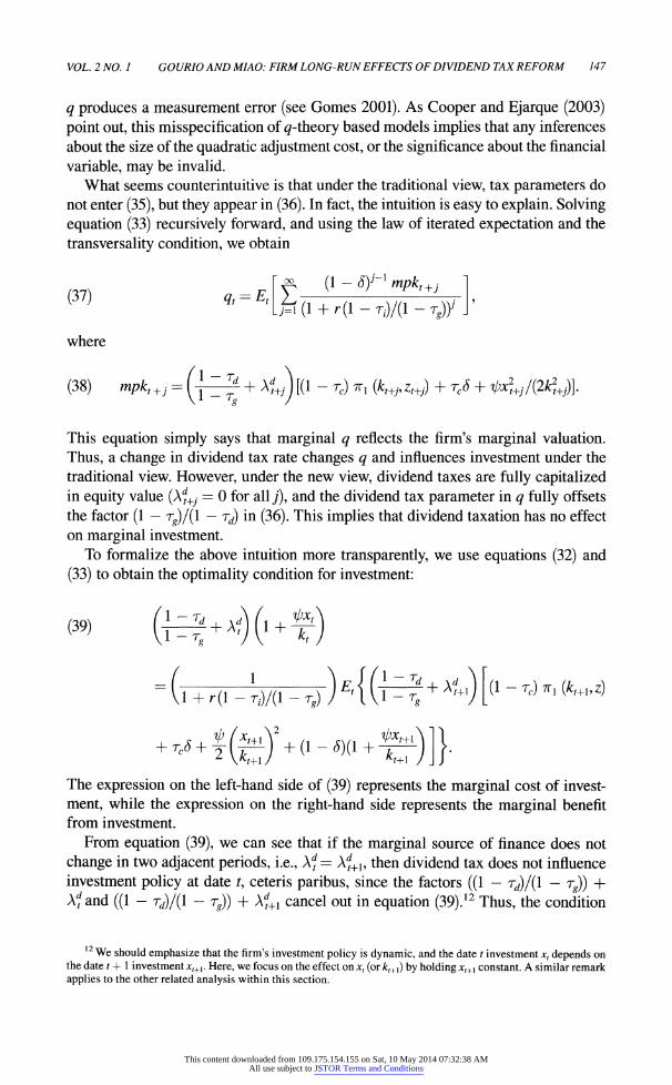
To formalize the above intuition more transparently, we use equations (32) and
(33) to obtain the optimality condition for investment:
(39) 1 -
T? fA? 1 +
1 + r(l -
r,.)/(l -
rg) t+\ (1
- Tc) ITi (kt+l,z)
+ TC5 + t _ 2 V*.
4+1
The expression on the left-hand side of (39) represents the marginal cost of invest
ment, while the expression on the right-hand side represents the marginal benefit from investment.
From equation (39), we can see that if the marginal source of finance does not
change in two adjacent periods, i.e., A? =
A?+1, then dividend tax does not influence investment policy at date t, ceteris paribus, since the factors ((1
- rd)/(l
- rg)) +
A? and ((1 -
rd)/(l -
rg)) + A?+1 cancel out in equation (39).12 Thus, the condition
12 We should emphasize that the firm's investment policy is dynamic, and the date t investment xt depends on
the date t + 1 investment xt+l. Here, we focus on the effect on xt (or kt+]) by holding xt+l constant. A similar remark applies to the other related analysis within this section.
This content downloaded from 109.175.154.155 on Sat, 10 May 2014 07:32:38 AMAll use subject to JSTOR Terms and Conditions
148 AMERICAN ECONOMIC JOURNAL: MACROECONOMICS JANUARY 2010
mc
l-Td l-Tt
MB3
0 (1
- rc) 7r(k, z) + Srck
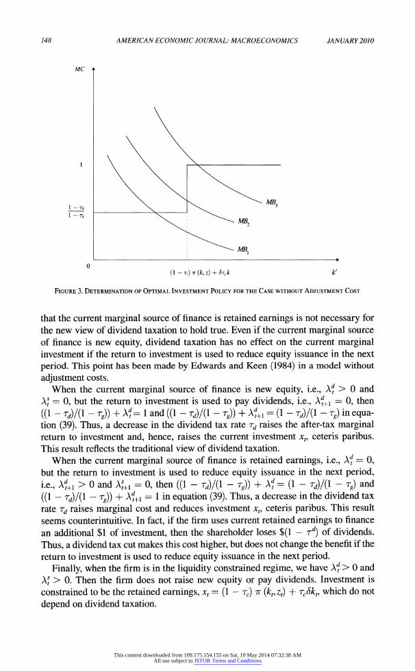
Figure 3. Determination of Optimal Investment Policy for the Case without Adjustment Cost
that the current marginal source of finance is retained earnings is not necessary for
the new view of dividend taxation to hold true. Even if the current marginal source
of finance is new equity, dividend taxation has no effect on the current marginal investment if the return to investment is used to reduce equity issuance in the next
period. This point has been made by Edwards and Keen (1984) in a model without
adjustment costs.
When the current marginal source of finance is new equity, i.e., Af > 0 and
Xst = 0, but the return to investment is used to pay dividends, i.e., Af+1
= 0, then
((1 -
rd)/(l -
rg)) + A? = 1 and ((1 -
r,)/(l -
rg)) + Af+1 = (1
- rd)/{\
- rg) in equa
tion (39). Thus, a decrease in the dividend tax rate rd raises the after-tax marginal return to investment and, hence, raises the current investment xt9 ceteris paribus. This result reflects the traditional view of dividend taxation.
When the current marginal source of finance is retained earnings, i.e., Af = 0,
but the return to investment is used to reduce equity issuance in the next period,
i.e., Af+1 > 0 and Af+1 - 0, then ((1 -
rd)/{\ -
rg)) + Af = (1 -
rd)/{l -
rg) and
((1 ?
rd)/(l ?
rg)) + Af+1 = 1 in equation (39). Thus, a decrease in the dividend tax
rate rd raises marginal cost and reduces investment xt, ceteris paribus. This result
seems counterintuitive. In fact, if the firm uses current retained earnings to finance
an additional $1 of investment, then the shareholder loses $(1 - of dividends.
Thus, a dividend tax cut makes this cost higher, but does not change the benefit if the
return to investment is used to reduce equity issuance in the next period.
Finally, when the firm is in the liquidity constrained regime, we have Af > 0 and
Xst > 0. Then the firm does not raise new equity or pay dividends. Investment is
constrained to be the retained earnings, xt ?
(1 ?
rc) tt (kt9zi) + rcSkt9 which do not
depend on dividend taxation.
This content downloaded from 109.175.154.155 on Sat, 10 May 2014 07:32:38 AMAll use subject to JSTOR Terms and Conditions
VOL. 2 NO. 1 GOURIO AND MIAO: FIRM LONG-RUN EFFECTS OF DIVIDEND TAX REFORM 149
Figure 3 illustrates the determination of the optimal investment policy for the
case without adjustment cost = 0). When the investment demand is low, as with
the MB1 schedule, investment spending can be financed from internal funds, at the
expense of extra dividends. The marginal cost is equal to (1 ?
rd)/(l ?
rg). By con
trast, for high investment demand, as with the MB3 schedule, the firm raises new
equity, and the marginal cost is equal to one. For an intermediate level of investment
demand, as with the MB2 schedule, the firm is constrained to invest at the amount
of retained earnings (1 ?
rc) it (k9z) + rc6k.
User Cost of Capital.?We can also analyze the effects of dividend taxation on
investment using the user cost of capital framework following Dale W. Jorgenson
(1963). To simplify the analysis, we only consider the deterministic case. We gener alize Andrew B. Abel's (1990) and Jorgenson's (1963) definition of the user cost of
capital to include adjustment cost and dividend taxation. We define the user cost of
capital as the cost ut, such that it is equal to the after-corporate-tax marginal cash
flow of an additional unit of capital, i.e.,
(40) H(=(1_r>1(^+l)+^|?Lj.
Using (33), we can derive that
(41) u, = + Af+1)
1 [q, (r (1 -
r,.)/(l -
rg) + 6)- Aq,(l -
5)} - 6rc,
where Aqt =
qt+x ?
qt. Thus, the user cost of capital is equal to the sum of the tax
adjusted interest rate, physical depreciation, and the capital loss, minus deprecia tion allowance. Importantly, it depends on the firm's dynamic finance regimes as
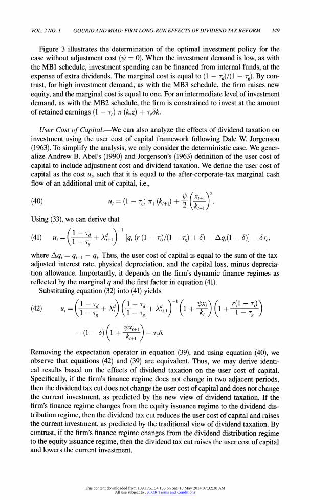
reflected by the marginal q and the first factor in equation (41). Substituting equation (32) into (41) yields
Removing the expectation operator in equation (39), and using equation (40), we
observe that equations (42) and (39) are equivalent. Thus, we may derive identi cal results based on the effects of dividend taxation on the user cost of capital. Specifically, if the firm's finance regime does not change in two adjacent periods, then the dividend tax cut does not change the user cost of capital and does not change the current investment, as predicted by the new view of dividend taxation. If the firm's finance regime changes from the equity issuance regime to the dividend dis tribution regime, then the dividend tax cut reduces the user cost of capital and raises the current investment, as predicted by the traditional view of dividend taxation. By contrast, if the firm's finance regime changes from the dividend distribution regime to the equity issuance regime, then the dividend tax cut raises the user cost of capital and lowers the current investment.
This content downloaded from 109.175.154.155 on Sat, 10 May 2014 07:32:38 AMAll use subject to JSTOR Terms and Conditions
150 AMERICAN ECONOMIC JOURNAL: MACROECONOMICS JANUARY 2010
We have pointed out before that if rd = rg, then the Miller-Modigliani dividend
irrelevance theorem holds, and Af =
Af+1 = 0. We can then use equation (42) to show
that a cut of the common tax rate rd = rg lowers the user cost of capital and raises
investment for a firm in any finance regime. This result is useful for understanding our policy experiments in Section IV.
C. Importance of Firm Heterogeneity
To understand the importance of heterogeneity in determining the steady-state effect of the dividend tax reform, we consider the case in which there is only one
representative firm in the model described in Section II. Also, we suppose there is no uncertainty. Because aggregate consumption in a steady state is constant over
time, equation (20) determines the interest rate. In addition, equations (31)?(33) still describe the representative firm's first-order conditions, except that we remove
the shock variable zt and the expectation operator. Because kt =
kt+h xt = 5kt, and
Af = A?+1 for all t in a deterministic steady state, it follows from (39) that the steady state capital stock k* satisfies
(43) 1 + # = 1 + (r(1
_ _ [(1 -
rc) 7rt (F) + rc5 + (#2/2)
+ (1 +#)(,-<*)].
This equation implies that in a model without firm heterogeneity, dividend taxation
does not influence the steady-state capital stock. This is because the representative firm can finance its investment using retained earnings in the deterministic steady state, and its finance regime does not change over time. By contrast, in our model
with firm heterogeneity, because of idiosyncratic productivity shocks, firms face dif
ferent finance regimes, and respond to a dividend tax cut in different ways. Thus, a
dividend tax cut will influence the steady-state capital stock. In the next section, we
analyze its quantitative effects.
IV. Quantitative Results
Now, we turn to the general equilibrium model presented in Section II. Because
this model does not permit a closed-form solution for the stationary equilibrium, we
resort to a numerical method to compute the approximate equilibrium. Appendix Section B details our numerical method.
A. Baseline Parametrization
To solve the model numerically, we need to specify functional forms for utility and technology. We also need to assign parameter values. We assume a time period in the model corresponds to one year. We calibrate our baseline model to match
some moments obtained from the COMPUSTAT database. The sample period
This content downloaded from 109.175.154.155 on Sat, 10 May 2014 07:32:38 AMAll use subject to JSTOR Terms and Conditions
VOL. 2 NO. 1 GOURIO AND Ml AO: FIRM LONG-RUN EFFECTS OF DIVIDEND TAX REFORM 151
ranges from 1988 to 2002, which corresponds to the period before the dividend tax
cut. Appendix Section A describes the data construction.
Tax System.?It is delicate to calibrate tax rates since in reality they are nonlinear
and change each year, while we have assumed constant and flat rates in our model.
In order to evaluate the 2003 dividend tax reform, we suppose that the initial steady state tax rates are given by the federal statutory rates in 2003 before the tax reform.
We set the corporate income tax rate rc = 0.34. Dividend tax rate, personal income tax rate, and capital gains tax rate depend on the individual's income tax bracket. We
suppose the representative household has an average income in the United States, which falls into the lowest of the top four tax brackets at the personal income tax
rate rt = 0.25. This household faces the capital gains tax rate rg = 0.20. Because
dividends are taxed at the personal income tax rate, we set rd ? 0.25.
Preferences.?We take the utility function:
(44) C/(c,L) = ln(c)-^,
where h > 0 is the weight on leisure. This utility function has a unit Frisch elasticity of labor supply, which is reasonable for macro models as argued by Robert E. Hall
(2008). We choose the discount factor (3 such that the interest rate r is equal to 0.04 using equation (20). We choose the parameter h to match the equilibrium labor sup
ply of 0.3, which is the average fraction of time spent on market work.
Technology.?We choose the Cobb-Douglas production function with decreas
ing returns to scale, F(kJ;z) = zka" la\ where 0 < ak^at < 1 and ak + at < 1. We
assume that the productivity shock follows the process,
(45) In zt = p In zt-i + et,
where et is independently and identically distributed and normally distributed with mean zero and variance a2. In Appendix Section C, we detail the procedure for
calibrating the parameter values ah ah p, and o. We find p ? 0.767, a = 0.211,
ak = 0.311, and al = 0.650. These estimates are similar to those in Cooper and
Haltiwanger (2006), Gomes (2001), and Hennessy and Whited (2005). We set the depreciation rate to match the aggregate investment-capital ratio, which is equal to 0.095 according to the National Income and Product Accounts.
The final parameter to be calibrated is the adjustment cost parameter ip. Because the volatility (standard deviation) of the investment rate is very sensitive to this parameter, we choose a value to match the cross-sectional volatility of the invest ment rate in our data, which is 0.156. More specifically, for any given value of ̂ , we solve the model numerically and obtain the stationary distribution of firms.
Using this stationary distribution, we compute the cross-sectional standard devia tion of the investment rate in the model. If there were no adjustment cost, our model
would imply excessive sensitivity of investment to variations in productivity shocks, which is inconsistent with empirical evidence. Our calibrated value of t/j is equal to
This content downloaded from 109.175.154.155 on Sat, 10 May 2014 07:32:38 AMAll use subject to JSTOR Terms and Conditions
152 AMERICAN ECONOMIC JOURNAL: MACROECONOMICS JANUARY 2010
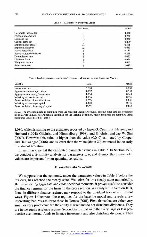
Table 3?Baseline Parametrization
Parameter Value
Corporate income tax rc 0.340 Personal income tax 0.250
Dividend tax rd 0.250
Capital gains tax Tg 0.200
Exponent on capital ak 0.311
Exponent on labor a, 0.650 Shock persistence p 0.767 Shock standard deviation cr 0.211
Depreciation rate $ 0.095 Discount factor /3 0.971
Weight on leisure h 6.616
Adjustment cost ip 1.080
Table 4?Aggregate and Cross-Sectional Moments in the Baseline Model
Variable Data Model
Investment rate 0.095 0.095
Aggregate dividends/earnings 0.137 0.353
Aggregate new equity/investment 0.130 0.148
Volatility of investment rate 0.156 0.156 Autocorrelation of investment rate 0.596 0.648
Volatility of earnings/capital 0.623 0.175
Autocorrelation of earnings/capital 0.791 0.658
Notes: The investment rate is computed from the National Income Accounts, and the other data are computed
using COMPUSTAT. See Appendix Section B for the variable definition. Model moments are computed using parameter values listed in Table 3.
1.080, which is similar to the estimates reported by Jason G. Cummins, Hassett, and
Hubbard (1994); Gilchrist and Himmelberg (1998); and Gilchrist and Jae W. Sim
(2007). However, this value is higher than the value (0.049) estimated by Cooper and Haltiwanger (2006), and is lower than the value (about 20) estimated in the early investment literature.
In summary, we list the calibrated parameter values in Table 3. In Section IVE, we conduct a sensitivity analysis for parameters p, cr, and ip since these parameter values are important for our quantitative results.
B. Baseline Model Results
We suppose that the economy, under the parameter values in Table 3 before the
tax cuts, has reached the steady state. We solve for this steady state numerically. Before reporting aggregate and cross sectional moments, it proves useful to consider
the finance regimes for the firms in the cross section. As analyzed in Section IIIB, firms in different finance regimes may respond to the dividend tax cut in different
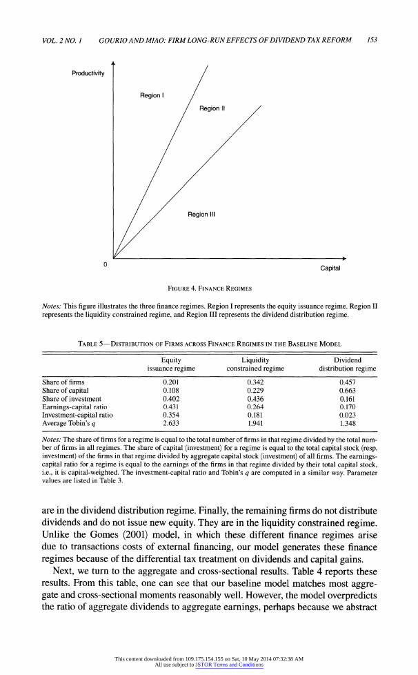
ways. Figure 4 illustrates these regimes for the baseline model and reveals a few
interesting features similar to those in Gomes (2001). First, firms that are either very small or very productive tap the equity market and do not distribute dividends. They are in the equity issuance regime. Second, firms that are either very large or less pro ductive use internal funds to finance investment and also distribute dividends. They
This content downloaded from 109.175.154.155 on Sat, 10 May 2014 07:32:38 AMAll use subject to JSTOR Terms and Conditions
VOL. 2 NO. 1 G0URI0 AND MI AO: FIRM LONG-RUN EFFECTS OF DIVIDEND TAX REFORM 153
Productivity
Capital
Figure 4. Finance Regimes
Notes: This figure illustrates the three finance regimes. Region I represents the equity issuance regime. Region II
represents the liquidity constrained regime, and Region III represents the dividend distribution regime.
Table 5?Distribution of Firms across Finance Regimes in the Baseline Model
Equity issuance regime
Liquidity constrained regime
Dividend distribution regime
Share of firms Share of capital Share of investment
Earnings-capital ratio
Investment-capital ratio
Average Tobin's q
0.201 0.108 0.402 0.431 0.354 2.633
0.342 0.229 0.436 0.264 0.181 1.941
0.457 0.663 0.161 0.170 0.023 1.348
Notes: The share of firms for a regime is equal to the total number of firms in that regime divided by the total num ber of firms in all regimes. The share of capital (investment) for a regime is equal to the total capital stock (resp. investment) of the firms in that regime divided by aggregate capital stock (investment) of all firms. The earnings capital ratio for a regime is equal to the earnings of the firms in that regime divided by their total capital stock, i.e., it is capital-weighted. The investment-capital ratio and Tobin's q are computed in a similar way. Parameter values are listed in Table 3.
are in the dividend distribution regime. Finally, the remaining firms do not distribute dividends and do not issue new equity. They are in the liquidity constrained regime. Unlike the Gomes (2001) model, in which these different finance regimes arise due to transactions costs of external financing, our model generates these finance
regimes because of the differential tax treatment on dividends and capital gains. Next, we turn to the aggregate and cross-sectional results. Table 4 reports these
results. From this table, one can see that our baseline model matches most aggre gate and cross-sectional moments reasonably well. However, the model overpredicts the ratio of aggregate dividends to aggregate earnings, perhaps because we abstract
This content downloaded from 109.175.154.155 on Sat, 10 May 2014 07:32:38 AMAll use subject to JSTOR Terms and Conditions
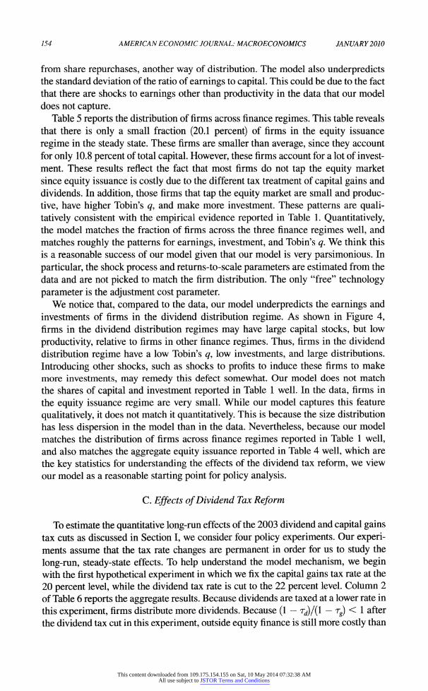
154 AMERICAN ECONOMIC JOURNAL: MACROECONOMICS JANUARY 2010
from share repurchases, another way of distribution. The model also underpredicts the standard deviation of the ratio of earnings to capital. This could be due to the fact
that there are shocks to earnings other than productivity in the data that our model
does not capture. Table 5 reports the distribution of firms across finance regimes. This table reveals
that there is only a small fraction (20.1 percent) of firms in the equity issuance
regime in the steady state. These firms are smaller than average, since they account
for only 10.8 percent of total capital. However, these firms account for a lot of invest
ment. These results reflect the fact that most firms do not tap the equity market
since equity issuance is costly due to the different tax treatment of capital gains and
dividends. In addition, those firms that tap the equity market are small and produc tive, have higher Tobin's q, and make more investment. These patterns are quali
tatively consistent with the empirical evidence reported in Table 1. Quantitatively, the model matches the fraction of firms across the three finance regimes well, and
matches roughly the patterns for earnings, investment, and Tobin's q. We think this
is a reasonable success of our model given that our model is very parsimonious. In
particular, the shock process and returns-to-scale parameters are estimated from the
data and are not picked to match the firm distribution. The only "free" technology
parameter is the adjustment cost parameter. We notice that, compared to the data, our model underpredicts the earnings and
investments of firms in the dividend distribution regime. As shown in Figure 4, firms in the dividend distribution regimes may have large capital stocks, but low
productivity, relative to firms in other finance regimes. Thus, firms in the dividend
distribution regime have a low Tobin's q, low investments, and large distributions.
Introducing other shocks, such as shocks to profits to induce these firms to make more investments, may remedy this defect somewhat. Our model does not match
the shares of capital and investment reported in Table 1 well. In the data, firms in
the equity issuance regime are very small. While our model captures this feature
qualitatively, it does not match it quantitatively. This is because the size distribution
has less dispersion in the model than in the data. Nevertheless, because our model
matches the distribution of firms across finance regimes reported in Table 1 well, and also matches the aggregate equity issuance reported in Table 4 well, which are
the key statistics for understanding the effects of the dividend tax reform, we view
our model as a reasonable starting point for policy analysis.
C. Effects of Dividend Tax Reform
To estimate the quantitative long-run effects of the 2003 dividend and capital gains tax cuts as discussed in Section I, we consider four policy experiments. Our experi
ments assume that the tax rate changes are permanent in order for us to study the
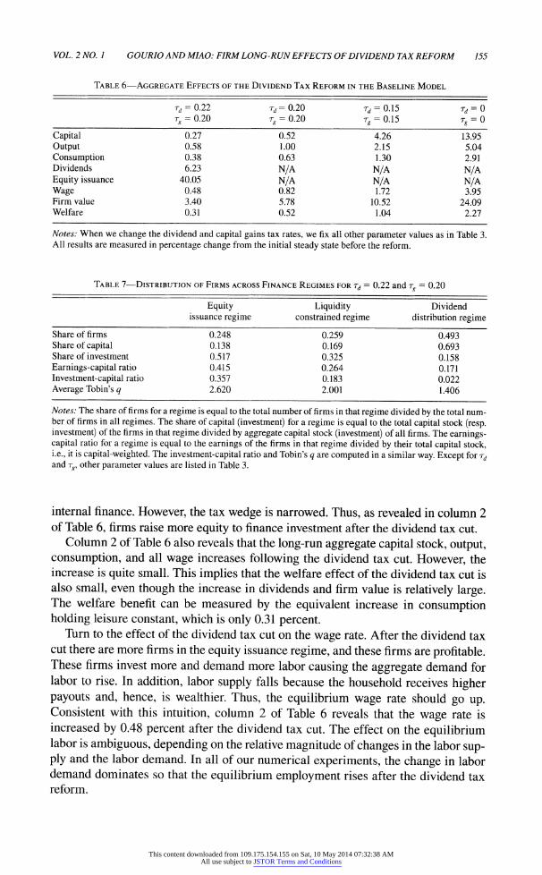
long-run, steady-state effects. To help understand the model mechanism, we begin with the first hypothetical experiment in which we fix the capital gains tax rate at the
20 percent level, while the dividend tax rate is cut to the 22 percent level. Column 2
of Table 6 reports the aggregate results. Because dividends are taxed at a lower rate in
this experiment, firms distribute more dividends. Because (1 ?
rrf)/(l ?
rg) < 1 after
the dividend tax cut in this experiment, outside equity finance is still more costly than
This content downloaded from 109.175.154.155 on Sat, 10 May 2014 07:32:38 AMAll use subject to JSTOR Terms and Conditions
VOL. 2 NO. 1 GOURIO AND MIAO: FIRM LONG-RUN EFFECTS OF DIVIDEND TAX REFORM
Table 6?Aggregate Effects of the Dividend Tax Reform in the Baseline Model
155
rd = 022 rd=0.20 Td
= 0.\5 rd = 0
Tg = Q.2Q 7-^
= 0.20 tg = 0.15 rg
= 0
Capital 0.27 0.52 4.26 13.95 Output 0.58 1.00 2.15 5.04 Consumption 0.38 0.63 1.30 2.91 Dividends 6.23 N/A N/A N/A Equity issuance 40.05 N/A N/A N/A Wage 0.48 0.82 1.72 3.95 Firm value 3.40 5.78 10.52 24.09 Welfare 0.31 0.52 1.04 2.27
Notes: When we change the dividend and capital gains tax rates, we fix all other parameter values as in Table 3. All results are measured in percentage change from the initial steady state before the reform.
Table 7?Distribution of Firms across Finance Regimes for rd = 0.22 and rg
= 0.20
Equity Liquidity Dividend issuance regime constrained regime distribution regime
Share of firms 0.248 0.259 0493 Share of capital 0.138 0.169 0.693 Share of investment 0.517 0.325 0.158
Earnings-capital ratio 0.415 0.264 0.171
Investment-capital ratio 0.357 0.183 0.022
Average Tobin's q 2.620 2.001 1.406
Notes: The share of firms for a regime is equal to the total number of firms in that regime divided by the total num ber of firms in all regimes. The share of capital (investment) for a regime is equal to the total capital stock (resp. investment) of the firms in that regime divided by aggregate capital stock (investment) of all firms. The earnings capital ratio for a regime is equal to the earnings of the firms in that regime divided by their total capital stock, i.e., it is capital-weighted. The investment-capital ratio and Tobin's q are computed in a similar way. Except for rd and rg, other parameter values are listed in Table 3.
internal finance. However, the tax wedge is narrowed. Thus, as revealed in column 2 of Table 6, firms raise more equity to finance investment after the dividend tax cut.
Column 2 of Table 6 also reveals that the long-run aggregate capital stock, output, consumption, and all wage increases following the dividend tax cut. However, the increase is quite small. This implies that the welfare effect of the dividend tax cut is also small, even though the increase in dividends and firm value is relatively large. The welfare benefit can be measured by the equivalent increase in consumption holding leisure constant, which is only 0.31 percent.
Turn to the effect of the dividend tax cut on the wage rate. After the dividend tax cut there are more firms in the equity issuance regime, and these firms are profitable. These firms invest more and demand more labor causing the aggregate demand for labor to rise. In addition, labor supply falls because the household receives higher payouts and, hence, is wealthier. Thus, the equilibrium wage rate should go up. Consistent with this intuition, column 2 of Table 6 reveals that the wage rate is increased by 0.48 percent after the dividend tax cut. The effect on the equilibrium labor is ambiguous, depending on the relative magnitude of changes in the labor sup ply and the labor demand. In all of our numerical experiments, the change in labor demand dominates so that the equilibrium employment rises after the dividend tax reform.
This content downloaded from 109.175.154.155 on Sat, 10 May 2014 07:32:38 AMAll use subject to JSTOR Terms and Conditions
756 AMERICAN ECONOMIC JOURNAL: MACROECONOMICS JANUARY 2010
To understand the effect on aggregate capital accumulation, we recall that firm
heterogeneity plays a key role. As shown in Section IIIC, if there was no firm het
erogeneity, dividend taxes would have no effect on the steady-state capital stock.
Table 7 illustrates the importance of firm heterogeneity. Compared with Table 5, Table 7 reveals that after the dividend tax cut, fewer firms are constrained. That is, some firms in the liquidity constrained regime move to the equity issuance regime, and some firms move to the dividend distribution regime. The firms in the equity issuance regime account for most of the increase in investment. The behavior of these firms is consistent with the traditional view of dividend taxation. The changes in the cross-sectional distribution of firms are consistent with the empirical results
reported in Section I.
Next, we consider the second policy experiment in which we fix the capital gains tax rate at the 20 percent level, while the dividend tax rate is cut to the 20 percent level. As a result, firms do not face the tax differential cost of external equity finance. Because there is no other friction associated with external equity finance
in the baseline model, the celebrated Miller and Modigliani (1961) dividend policy irrelevance theorem holds, as analyzed in Section IIIA. Thus, in column 3 of Table
6, the values of aggregate dividends and new equity are indeterminate (marked as
"N/A" ). Because firms do not face any financing frictions after the second policy
experiment, the long-run aggregate capital stock, output, consumption, and wage all increase more than that in the first policy experiment. In particular, aggregate
capital is raised by 0.52 percent, and aggregate output is raised by 1 percent. The
welfare increase measured by the increase in aggregate consumption is still small,
equal to 0.52 percent. We, now, consider the third policy experiment in which both the capital gains
tax rate and the dividend tax rate are cut permanently to the same level of 15 per cent. These tax cuts are implemented by JGTRRA. Column 4 of Table 6 reports the results. Compared with the second policy experiment reported in column 3, we
can see that the increases in aggregate capital, output, consumption, and wage are
higher. In particular, aggregate capital and welfare increase by 4.26 and 1.04 per cent, respectively. This larger effect is caused by a different channel in addition to
the preceding reallocation channel. From (8) or (26), we can see that the after-tax
interest rate is given by r(l ?
rf)/(l ?
rg). Thus, a decrease in rg ?
rd lowers the
after-tax interest rate and, hence, the user cost of capital for all firms, as analyzed in Section IIIB. Our numerical experiments illustrate that this channel has a larger
impact than the reallocation channel.
We conduct the fourth experiment in which both dividend and capital gains taxes
are eliminated permanently. We find a much larger impact on the economy, because
there is a large decrease in the user cost of capital for all firms in the economy. In
particular, aggregate capital increases by 13.95 percent and welfare increases by 2.27 percent.
D. Productivity Gains
We have shown that a dividend tax cut stimulates long-run capital formation in our
model with firm heterogeneity. In our model, firms with high productivity but with
This content downloaded from 109.175.154.155 on Sat, 10 May 2014 07:32:38 AMAll use subject to JSTOR Terms and Conditions
VOL. 2 NO. 1 GOURIO AND MIAO: FIRM LONG-RUN EFFECTS OF DIVIDEND TAX REFORM 157
little capital issue new equity. These firms are primarily responsible for the increase
in investment after the dividend tax cut. When the dividend tax is reduced, some
liquidity constrained firms move to the equity issuance regimes and they attract
more capital and labor. Hence, the allocation of capital and labor is more efficient, which generates productivity gains.
To gauge the productivity gains quantitatively, we use two measures: aggregate labor productivity (Y/L) and total factor productivity (Y/(KakLa')). To focus on the effect of dividend taxes alone, we consider the changes of rd from 0.25 to 0.22 and
0.20, and fix all other parameter values as in Table 3. Table 8 reports the results.
Row 2 of Table 8 reveals that total factor productivity (TFP) increases following the decrease in the dividend tax rate. To see the intuition, we use the Cobb-Douglas
production function to derive TFP as follows:
Y _U (&?k) W~ai V {dKdz)]
l~ai _ E(1 [z1/(1-^ ka^l-ai)]l-a>
(46) TFP = -^qji- ^(JMz)p "
(fi^
where and Cov^ denote the expectation and covariance operators for the stationary distribution of firms respecitively. The covariance term represents the reallocation
effect, which captures the fact that capital may move among firms with different
productivity shocks. If there were no reallocation effect, the covariance term would
be zero. If, in addition, production had constant returns to scale ak ? 1 ? ah then
TFP would be equal to {E^[zx^k])a\ which would not change following a change in the dividend tax rate. However, we have assumed decreasing returns to scale in our
model.13 In addition, row 4 of Table 8 reveals that the correlation between capital and productivity shock is positive and increases following a decrease in the dividend tax rate. Clearly, the higher this correlation, the more efficient the allocation of capi tal across firms. Row 5 shows that the slope coefficient in a regression of log capital on log firm productivity also increases, reflecting that firms with high productivity have relatively more capital. Thus, we should expect that TFP will increase if the
dividend tax rate is lowered. This intuition is confirmed in row 2 of Table 8.
We now turn to row 3 of Table 8, which reveals that labor productivity (Y/L) increases as the dividend tax rate decreases. To see the intuition, we use the Cobb
Douglas production function to compute labor productivity as follows:
(47) Y= /(Zr')1/^a'V(^^z)(a//w)a'/(1-Q') =J^ L
f(zka>)m-ai ?(dk,dz)(a,MW~ad ai'
13 Urban J. Jermann and Vincenzo Quadrini (2007) use a model with financial frictions and decreasing returns
to scale in production to explain the productivity gains in the 1990s. Unlike our model with taxation, they assume financial frictions are generated by the enforcement problem of lending contracts.
This content downloaded from 109.175.154.155 on Sat, 10 May 2014 07:32:38 AMAll use subject to JSTOR Terms and Conditions
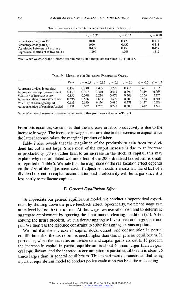
158 AMERICAN ECONOMIC JOURNAL: MACROECONOMICS JANUARY 2010
Table 8?Productivity Gains from the Dividend Tax Cut
rd = 0.25 rd
= 0.22 rd = 0.20
Percentage change in TFP 0.00 0.479 0.721
Percentage change in Y/L 0.00 0.430 0.818
Correlation between In k and In z 0.438 0.450 0.457
Regression coefficient of In k on In z 1.203 1.268 1.312
Note: When we change the dividend tax rate, we fix all other parameter values as in Table 3.
Table 9?Moments for Different Parameter Values
Data p = 0.65 p
= 0.85 a = 0.1 a = 0.3 ^ = 0.5 rj>
= 1-5
Aggregate dividends/earnings 0.137 0.290 0.435 0.296 0.413 0.481 0.315
Aggregate new equity/investment 0.130 0.007 0.340 0.010 0.294 0.419 0.069
Volatility of investment rate 0.156 0.098 0.224 0.076 0.208 0.254 0.127
Autocorrelation of investment rate 0.596 0.566 0.683 0.690 0.603 0.588 0.668
Volatility of earnings/capital 0.623 0.160 0.176 0.080 0.273 0.157 0.186
Autocorrelation of earnings/capital 0.791 0.557 0.732 0.720 0.588 0.647 0.662
Note: When we change one parameter value, we fix other parameter values as in Table 3.
From this equation, we can see that the increase in labor productivity is due to the
increase in wage. The increase in wage is, in turn, due to the increase in capital since
the latter increase raises the marginal product of labor.
Table 8 also reveals that the magnitude of the productivity gain from the divi
dend tax cut is not large. Since most of the output increase is due to an increase
in productivity (TFP), rather than to an increase in the stock of capital, this may
explain why our simulated welfare effect of the 2003 dividend tax reform is small, as reported in Table 6. We note that the magnitude of the reallocation effect depends on the size of the adjustment cost. If adjustment costs are smaller, the effect of a
dividend tax cut on capital accumulation and productivity will be larger since it is
less costly to reallocate capital.
E. General Equilibrium Effect
To appreciate our general equilibrium model, we conduct a hypothetical experi ment by shutting down the price feedback effect. Specifically, we fix the wage rate
at its level before the tax reform. At this wage, we use labor demand to determine
aggregate employment by ignoring the labor market-clearing condition (24). After
solving the firm's problem, we can derive aggregate investment and aggregate out
put. We then use the resource constraint to solve for aggregate consumption. We find that the increase in capital stock, output, and consumption in partial
equilibrium after the tax reform is much higher than that in general equilibrium. In
particular, when the tax rates on dividends and capital gains are cut to 15 percent, the increase in capital in partial equilibrium is about 6 times larger than in gen eral equilibrium, and the increase in consumption in partial equilibrium is about 26
times larger than in general equilibrium. This experiment demonstrates that using a partial equilibrium model to conduct policy evaluation can be quite misleading.
This content downloaded from 109.175.154.155 on Sat, 10 May 2014 07:32:38 AMAll use subject to JSTOR Terms and Conditions
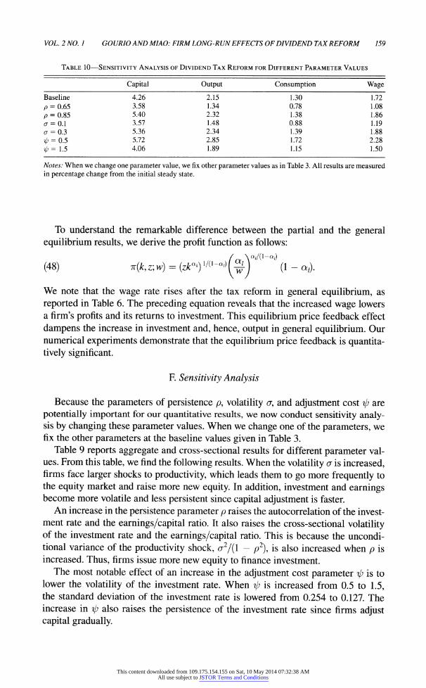
VOL. 2 NO. 1
Table 10
GOURIO AND MIAO: FIRM LONG-RUN EFFECTS OF DIVIDEND TAX REFORM
>?Sensitivity Analysis of Dividend Tax Reform for Different Parameter Values
159
Capital Output Consumption Wage
Baseline 4.26 2.15 1.30 1.72
p = 0.65 3.58 1.34 0.78 1.08
p = 0.85 5.40 2.32 1.38 1.86
(7 = 0.1 3.57 1.48 0.88 1.19 a = 03 5.36 2.34 1.39 1.88
^ = 0.5 5.72 2.85 1.72 2.28
xj) = 1.5 4.06 1.89 1.15 1.50
Notes: When we change one parameter value, we fix other parameter values as in Table 3. All results are measured in percentage change from the initial steady state.
To understand the remarkable difference between the partial and the general equilibrium results, we derive the profit function as follows:
(48) 7r(*,z;w) = (zk^Y^^j
(1 - a,). We note that the wage rate rises after the tax reform in general equilibrium, as
reported in Table 6. The preceding equation reveals that the increased wage lowers a firm's profits and its returns to investment. This equilibrium price feedback effect
dampens the increase in investment and, hence, output in general equilibrium. Our numerical experiments demonstrate that the equilibrium price feedback is quantita tively significant.
F. Sensitivity Analysis
Because the parameters of persistence p, volatility a, and adjustment cost if; are
potentially important for our quantitative results, we now conduct sensitivity analy sis by changing these parameter values. When we change one of the parameters, we fix the other parameters at the baseline values given in Table 3.
Table 9 reports aggregate and cross-sectional results for different parameter val ues. From this table, we find the following results. When the volatility a is increased, firms face larger shocks to productivity, which leads them to go more frequently to the equity market and raise more new equity. In addition, investment and earnings become more volatile and less persistent since capital adjustment is faster.
An increase in the persistence parameter p raises the autocorrelation of the invest ment rate and the earnings/capital ratio. It also raises the cross-sectional volatility of the investment rate and the earnings/capital ratio. This is because the uncondi tional variance of the productivity shock, o2/(l
? p2), is also increased when p is
increased. Thus, firms issue more new equity to finance investment. The most notable effect of an increase in the adjustment cost parameter ip is to
lower the volatility of the investment rate. When if; is increased from 0.5 to 1.5, the standard deviation of the investment rate is lowered from 0.254 to 0.127. The increase in ip also raises the persistence of the investment rate since firms adjust capital gradually.
This content downloaded from 109.175.154.155 on Sat, 10 May 2014 07:32:38 AMAll use subject to JSTOR Terms and Conditions
160 AMERICAN ECONOMIC JOURNAL: MACROECONOMICS JANUARY 2010
Table 10 reports the results when the tax rates are cut to rd = rg ? 0.15. This
table reveals that our estimates of the effects on capital, output, and consumption in
the baseline model are not very sensitive to the choice of parameter values. In par
ticular, for a wide range of parameter values, the steady-state capital stock and out
put increase by 3-6 percent and 1-3 percent, respectively. Notably, the steady-state increase in consumption is almost always below 2 percent. When the adjustment cost
parameter is small = 0.5), the reallocation effect and productivity gains from the
tax cut are large, as discussed in Section HID. In this case, the resulting increases in
aggregate output, capital, and consumption are relatively large.
V. Extensions
In this section, we consider extensions of our baseline model by relaxing some of
our previous assumptions. First, we consider a revenue-neutral tax reform. Second, we introduce debt financing. Third, we consider the effect of transaction costs of
equity issuance. Finally, we allow for share repurchases. When we relax one assump
tion, we hold everything else constant as in the baseline model. We show that our
estimates of the benefit from the 2003 dividend tax cut will be reduced in these extensions.
A. Revenue-Neutral Tax Reform
Our baseline model assumes tax revenues are rebated back to the household. Tax
revenues must decrease after a dividend and capital gains tax cut. This means that
the household receives smaller lump-sum transfers from the government. If the gov ernment tries to keep tax revenues constant after a dividend and capital gains tax cut,
it must raise other taxes. If the increased taxes are distortionary, the benefit from a
dividend and capital gains tax cut will be reduced.
To illustrate this point quantitatively, we consider an experiment in which the
government raises the personal (labor) income tax rate to keep tax revenues iden
tical to the level before the tax cut. We find that the equilibrium tax revenues are
reduced by 3.1 percent after the dividend and capital gains tax rates are cut to rd =
rg = 0.15 from their baseline values. To restore tax revenues to their level before
the tax cut, the government must raise the tax rate on labor income to r( = 0.266,
1.6 percentage points higher than the level before the tax cut. This higher labor
income tax rate distorts labor supply and thus reduces the benefit from the dividend
and capital gains tax cut. In particular, we find that aggregate capital, output, and
consumption increase by 3.23, 1.16, and 0.30 percent, respectively. These numbers
are all smaller than the corresponding values (4.26, 2.15, and 1.30 percent) in our
baseline model.
B. Debt Financing
Our baseline model assumes that the only source of outside financing is equity.
However, firms also rely on debt to finance investment (either through the bond
market or through bank loans). In this section, we introduce debt financing in the
This content downloaded from 109.175.154.155 on Sat, 10 May 2014 07:32:38 AMAll use subject to JSTOR Terms and Conditions
VOL. 2 NO. 1 GOURIO AND MIAO: FIRM LONG-RUN EFFECTS OF DIVIDEND TAX REFORM 161
model to study how it affects our results. We follow Poterba and Summers (1983), and assume that debt is risk-free and is equal to a fixed fraction of capital, bt
? ?jkt.
This assumption may be motived by a binding collateral constraint as in Nobuhiro
Kiyotaki and John Moore (1997).14 As a firm accumulates more capital, it raises its debt capacity, in that capital is tantamount to collateral. This simple formulation
simplifies our numerical solution since we still solve the dynamic programming
problem (8), but the flow of funds constraint (9) is modified to be:
ibx2 (49) x + + d + (1 + (1
- rc)r)b = (1
- rc) tt (k,z\w) + rc6k + s + b',
(50) b = ?k9 b' = &'.
To illustrate how our results are affected by this modification, we keep the same
parameter values as in Table 3, and set ? = 0.5. This number is in the range of
estimates reported by Valerie A. Ramey and Shapiro (2001), and is close to the estimates of Hennessy and Whited (2005). We find that equity issuance becomes smaller, because firms can access debt financing rather than only using internal funds or equity issuance. The ratio of equity issuance to investment is 5 percent rather than 14.8 percent. In addition, there are fewer firms issuing equity (14.9 per cent rather than 20.1 percent).
We next analyze the effects of the dividend tax cut by conducting experiments similar to Table 6. We find that the effects on the wage, consumption, and equity issuance are smaller than in the baseline model. This is because the reallocation effect is smaller with debt financing. We also find that the increase in capital in the model with debt financing is a little larger than in the baseline model when we
reduce rd alone to 0.20 (0.71 percent versus 0.52 percent), but is a little smaller than in the baseline model when we reduce both rg and rd to 0.15 (2.81 percent versus 4.26
percent). The intuition appears to be the following. On the one hand, when firms can issue debt, they rely less on equity financing. Thus, reducing dividend taxes should have a smaller effect than in the baseline model without debt financing. On the other hand, an increase in capital in the model with debt relaxes the collateral constraint and allows firms to take on more debt, thereby stimulating more capital accumulation. For small tax changes, the second effect dominates, but for large tax
changes, the first effect dominates.
C. Costly External Finance
So far, we have assumed that external equity finance is costly only because of the differential tax treatment on capital gains and dividends. Many researchers
14 In the case with occasionally binding collateral constraint, as in Hennessy and Whited (2005) and Gourio and Miao (2007), debt is an additional state variable. Our dynamic programming problem becomes three dimen sional, which is harder to solve numerically.
This content downloaded from 109.175.154.155 on Sat, 10 May 2014 07:32:38 AMAll use subject to JSTOR Terms and Conditions
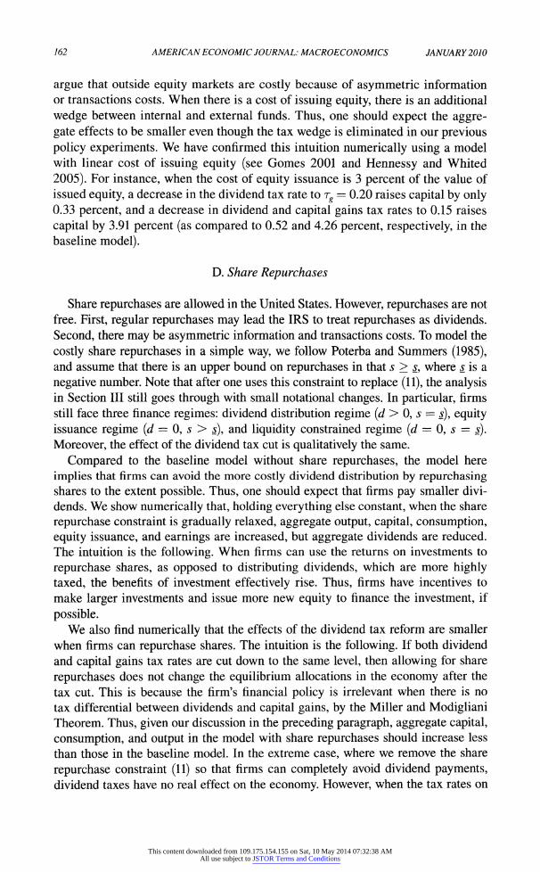
762 AMERICAN ECONOMIC JOURNAL: MACROECONOMICS JANUARY 2010
argue that outside equity markets are costly because of asymmetric information or transactions costs. When there is a cost of issuing equity, there is an additional
wedge between internal and external funds. Thus, one should expect the aggre
gate effects to be smaller even though the tax wedge is eliminated in our previous
policy experiments. We have confirmed this intuition numerically using a model
with linear cost of issuing equity (see Gomes 2001 and Hennessy and Whited
2005). For instance, when the cost of equity issuance is 3 percent of the value of
issued equity, a decrease in the dividend tax rate to rg = 0.20 raises capital by only
0.33 percent, and a decrease in dividend and capital gains tax rates to 0.15 raises
capital by 3.91 percent (as compared to 0.52 and 4.26 percent, respectively, in the
baseline model).
D. Share Repurchases
Share repurchases are allowed in the United States. However, repurchases are not
free. First, regular repurchases may lead the IRS to treat repurchases as dividends.
Second, there may be asymmetric information and transactions costs. To model the
costly share repurchases in a simple way, we follow Poterba and Summers (1985), and assume that there is an upper bound on repurchases in that s > s, where s is a
negative number. Note that after one uses this constraint to replace (11), the analysis in Section III still goes through with small notational changes. In particular, firms
still face three finance regimes: dividend distribution regime (d > 0, s = s), equity issuance regime (d
? 0, s > s), and liquidity constrained regime (d ? 0, s = s).
Moreover, the effect of the dividend tax cut is qualitatively the same.
Compared to the baseline model without share repurchases, the model here
implies that firms can avoid the more costly dividend distribution by repurchasing shares to the extent possible. Thus, one should expect that firms pay smaller divi
dends. We show numerically that, holding everything else constant, when the share
repurchase constraint is gradually relaxed, aggregate output, capital, consumption,
equity issuance, and earnings are increased, but aggregate dividends are reduced.
The intuition is the following. When firms can use the returns on investments to
repurchase shares, as opposed to distributing dividends, which are more highly taxed, the benefits of investment effectively rise. Thus, firms have incentives to
make larger investments and issue more new equity to finance the investment, if
possible. We also find numerically that the effects of the dividend tax reform are smaller
when firms can repurchase shares. The intuition is the following. If both dividend
and capital gains tax rates are cut down to the same level, then allowing for share
repurchases does not change the equilibrium allocations in the economy after the
tax cut. This is because the firm's financial policy is irrelevant when there is no
tax differential between dividends and capital gains, by the Miller and Modigliani Theorem. Thus, given our discussion in the preceding paragraph, aggregate capital,
consumption, and output in the model with share repurchases should increase less
than those in the baseline model. In the extreme case, where we remove the share
repurchase constraint (11) so that firms can completely avoid dividend payments, dividend taxes have no real effect on the economy. However, when the tax rates on
This content downloaded from 109.175.154.155 on Sat, 10 May 2014 07:32:38 AMAll use subject to JSTOR Terms and Conditions
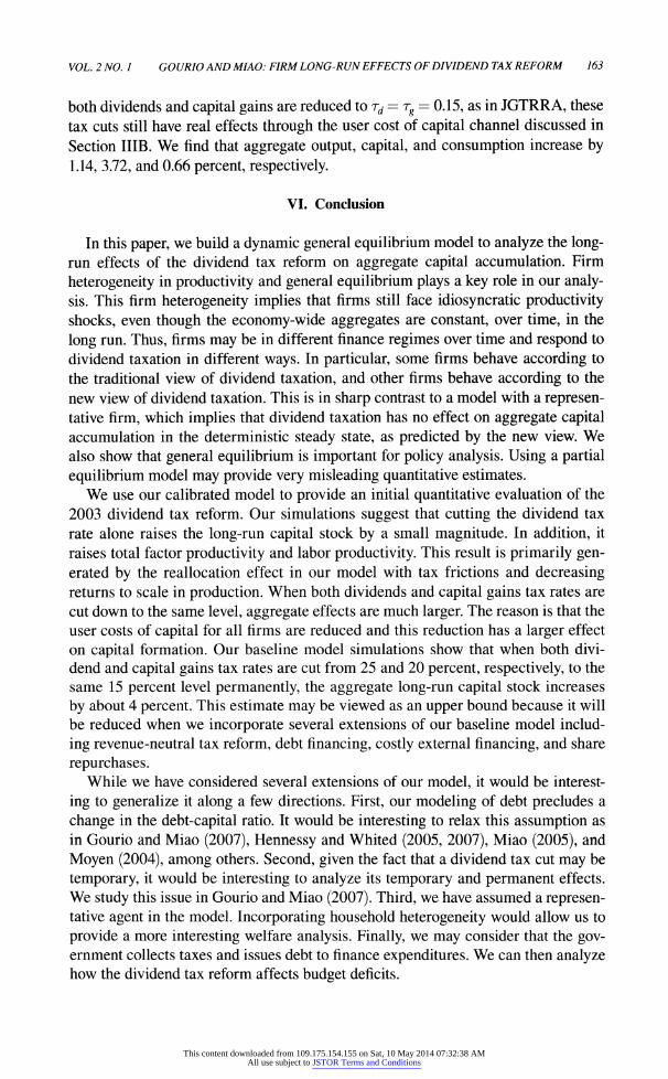
VOL. 2 NO. 1 GOURIO AND MI AO: FIRM LONG-RUN EFFECTS OF DIVIDEND TAX REFORM 163
both dividends and capital gains are reduced to rd ?
rg ? 0.15, as in JGTRRA, these
tax cuts still have real effects through the user cost of capital channel discussed in
Section IIIB. We find that aggregate output, capital, and consumption increase by
1.14, 3.72, and 0.66 percent, respectively.
VI. Conclusion
In this paper, we build a dynamic general equilibrium model to analyze the long run effects of the dividend tax reform on aggregate capital accumulation. Firm
heterogeneity in productivity and general equilibrium plays a key role in our analy sis. This firm heterogeneity implies that firms still face idiosyncratic productivity shocks, even though the economy-wide aggregates are constant, over time, in the
long run. Thus, firms may be in different finance regimes over time and respond to
dividend taxation in different ways. In particular, some firms behave according to
the traditional view of dividend taxation, and other firms behave according to the
new view of dividend taxation. This is in sharp contrast to a model with a represen tative firm, which implies that dividend taxation has no effect on aggregate capital accumulation in the deterministic steady state, as predicted by the new view. We
also show that general equilibrium is important for policy analysis. Using a partial
equilibrium model may provide very misleading quantitative estimates.
We use our calibrated model to provide an initial quantitative evaluation of the
2003 dividend tax reform. Our simulations suggest that cutting the dividend tax
rate alone raises the long-run capital stock by a small magnitude. In addition, it
raises total factor productivity and labor productivity. This result is primarily gen erated by the reallocation effect in our model with tax frictions and decreasing returns to scale in production. When both dividends and capital gains tax rates are
cut down to the same level, aggregate effects are much larger. The reason is that the
user costs of capital for all firms are reduced and this reduction has a larger effect
on capital formation. Our baseline model simulations show that when both divi
dend and capital gains tax rates are cut from 25 and 20 percent, respectively, to the
same 15 percent level permanently, the aggregate long-run capital stock increases
by about 4 percent. This estimate may be viewed as an upper bound because it will
be reduced when we incorporate several extensions of our baseline model includ
ing revenue-neutral tax reform, debt financing, costly external financing, and share
repurchases.
While we have considered several extensions of our model, it would be interest
ing to generalize it along a few directions. First, our modeling of debt precludes a
change in the debt-capital ratio. It would be interesting to relax this assumption as
in Gourio and Miao (2007), Hennessy and Whited (2005, 2007), Miao (2005), and Moyen (2004), among others. Second, given the fact that a dividend tax cut may be
temporary, it would be interesting to analyze its temporary and permanent effects.
We study this issue in Gourio and Miao (2007). Third, we have assumed a represen tative agent in the model. Incorporating household heterogeneity would allow us to
provide a more interesting welfare analysis. Finally, we may consider that the gov ernment collects taxes and issues debt to finance expenditures. We can then analyze how the dividend tax reform affects budget deficits.
This content downloaded from 109.175.154.155 on Sat, 10 May 2014 07:32:38 AMAll use subject to JSTOR Terms and Conditions
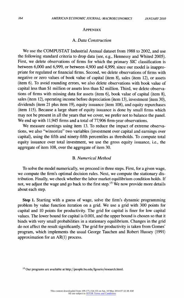
164 AMERICAN ECONOMIC JOURNAL: MACROECONOMICS JANUARY 2010
Appendix
A. Data Construction
We use the COMPUSTAT Industrial Annual dataset from 1988 to 2002, and use the following standard criteria to drop data (see, e.g., Hennessy and Whited 2005). First, we delete observations of firms for which the primary SIC classification is between 6,000 and 6,999, or between 4,900 and 4,999, since our model is inappro priate for regulated or financial firms. Second, we delete observations of firms with
negative or zero values of book value of capital (item 8), sales (item 12), or assets
(item 6). To avoid rounding errors, we also delete observations with book value of
capital less than $1 million or assets less than $2 million. Third, we delete observa tions of firms with missing data for assets (item 6), book value of capital (item 8), sales (item 12), operating income before depreciation (item 13), investment (item 30), dividends (item 21 plus item 19), equity issuance (item 108), and equity repurchases (item 115). Because a large share of equity issuance is done by small firms which
may not be present in all the years that we cover, we prefer not to balance the panel. We end up with 11,945 firms and a total of 77,906 firm-year observations.
We measure earnings using item 13. To reduce the impact of extreme observa
tions, we also "winsorize" two variables (investment over capital and earnings over
capital), using the fifth and ninety-fifth percentiles as thresholds. To compute total
equity issuance over total investment, we use the gross equity issuance, i.e., the
aggregate of item 108, over the aggregate of item 30.
B. Numerical Method
To solve the model numerically, we proceed in three steps. First, for a given wage, we compute the firm's optimal decision rules. Next, we compute the stationary dis
tribution. Finally, we check whether the labor market equilibrium condition holds. If
not, we adjust the wage and go back to the first step.15 We now provide more details
about each step.
Step 1. Starting with a guess of wage, solve the firm's dynamic programming
problem by value function iteration on a grid. We use a grid with 300 points for
capital and 10 points for productivity. The grid for capital is finer for low capital values. The lower bound for capital is 0.001, and the upper bound is chosen so that it
binds with very small probabilities in a stationary equilibrium. Changes in the grid do not affect the result significantly. The grid for productivity is taken from Gomes'
program, which implements the usual George Tauchen and Robert Hussey (1991)
approximation for an AR(1) process.
15 Our programs are available at http://people.bu.edu/fgourio/research.html.
This content downloaded from 109.175.154.155 on Sat, 10 May 2014 07:32:38 AMAll use subject to JSTOR Terms and Conditions
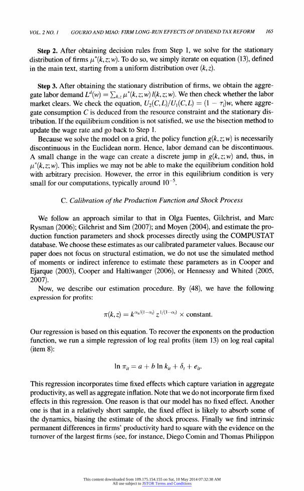
VOL. 2 NO. 1 G0URI0 AND MIAO: FIRM LONG-RUN EFFECTS OF DIVIDEND TAX REFORM 165
Step 2. After obtaining decision rules from Step 1, we solve for the stationary distribution of firms ii(k,z\w). To do so, we simply iterate on equation (13), defined in the main text, starting from a uniform distribution over (k,z).
Step 3. After obtaining the stationary distribution of firms, we obtain the aggre
gate labor demand Ld(w) =
Y,k,z & w) w)- We then check whether the labor market clears. We check the equation, U2(C9L)/Ul(C,L)
= (1
- t,)w, where aggre
gate consumption C is deduced from the resource constraint and the stationary dis
tribution. If the equilibrium condition is not satisfied, we use the bisection method to
update the wage rate and go back to Step 1.
Because we solve the model on a grid, the policy function g(k,z\w) is necessarily discontinuous in the Euclidean norm. Hence, labor demand can be discontinuous.
A small change in the wage can create a discrete jump in g(k9z\w) and, thus, in
H*(Kz\ w). This implies we may not be able to make the equilibrium condition hold with arbitrary precision. However, the error in this equilibrium condition is very small for our computations, typically around 10~5.
C. Calibration of the Production Function and Shock Process
We follow an approach similar to that in Olga Fuentes, Gilchrist, and Marc
Rysman (2006); Gilchrist and Sim (2007); and Moyen (2004), and estimate the pro duction function parameters and shock processes directly using the COMPUSTAT
database. We choose these estimates as our calibrated parameter values. Because our
paper does not focus on structural estimation, we do not use the simulated method
of moments or indirect inference to estimate these parameters as in Cooper and
Ejarque (2003), Cooper and Haltiwanger (2006), or Hennessy and Whited (2005, 2007).
Now, we describe our estimation procedure. By (48), we have the following
expression for profits:
tt(?,z) = k"^1-"1* zw~ai) x constant.
Our regression is based on this equation. To recover the exponents on the production function, we run a simple regression of log real profits (item 13) on log real capital
(item 8):
In 7rit ? a + b In kit + St + eit.
This regression incorporates time fixed effects which capture variation in aggregate
productivity, as well as aggregate inflation. Note that we do not incorporate firm fixed
effects in this regression. One reason is that our model has no fixed effect. Another one is that in a relatively short sample, the fixed effect is likely to absorb some of
the dynamics, biasing the estimate of the shock process. Finally we find intrinsic permanent differences in firms' productivity hard to square with the evidence on the turnover of the largest firms (see, for instance, Diego Comin and Thomas Philippon
This content downloaded from 109.175.154.155 on Sat, 10 May 2014 07:32:38 AMAll use subject to JSTOR Terms and Conditions
166 AMERICAN ECONOMIC JOURNAL: MACROECONOMICS JANUARY 2010
2005). We recognize, however, that the absence of firm fixed effects may increase
the endogeneity problem in this production function estimation.
Our estimate of b is b = 0.889. Following the macroeconomics literature, we set
at = 0.65, since labor share is approximately 65 percent in the US data. Given thatfe
is an estimate of ak/(\ ?
a,), this yields an estimate of ak: ak = 0.311.
We use the residuals from the regression to measure the shock process. We fit an
AR(1) to 77ff=(l -a^eit:
Vi,t =
PVi,t-\ +
where Qt is independently and identically distributed across i and t, and drawn from a standard normal distribution. These estimates imply that the parameters of the
shock process z are
p = 0.767, & = 0.211.
Overall, our estimates for parameters of the production function and the shock pro cess are quite similar to those in the papers previously cited.
REFERENCES
Abel, Andrew B. 1990. "Consumption and Investment." In Handbook of Monetary Economics Vol
ume 2, ed. B. M. Friedman and F. H. Hahn, 726-75. Amsterdam: Elsevier Science.
Auerbach, Alan J. 1979a. "Share Valuation and Corporate Equity Policy." Journal of Public Econom
ics, 11(3): 291-305. Auerbach, Alan J. 1979b. "Wealth Maximization and the Cost of Capital." Quarterly Journal of Eco
nomics, 93(3): 433-46. Auerbach, Alan J. 2002. "Taxation and Corporate Financial Policy." In Handbook of Public Econom
ics Volume 3, ed. Alan J. Auerbach and Martin Feldstein, 1251-92. Amsterdam: Elsevier Science.
Auerbach, Alan J., and Kevin A. Hassett. 2003. "On the Marginal Source of Investment Funds."
Journal of Public Economics, 87(1): 205-32. Auerbach, Alan J., and Laurence J. Kotlikoff. 1987. Dynamic Fiscal Policy. New York: Cambridge
University Press.
Barclay, Michael J., and Clifford W. Smith, Jr. 1988. "Corporate Payout Policy: Cash Dividends ver
sus Open-Market Repurchases." Journal of Financial Economics, 22(1): 61-82.
Barro, Robert J. 1989. "The Neoclassical Approach to Fiscal Policy." In Modern Business Cycle The
ory, ed. Robert J. Barro, 178-235. Cambridge, MA: Harvard University Press.
Bartelsman, Eric J., and Mark Doms. 2000. "Understanding Productivity: Lessons from Longitudi nal Microdata." Journal of Economic Literature, 38(3): 569-94.
Baxter, Marianne, and Robert G. King. 1993. "Fiscal Policy in General Equilibrium." American Eco
nomic Review, 83(3): 315-34. Bhattacharya, Sudipto. 1979. "Imperfect Information, Dividend Policy, and 'The Bird in the Hand'
Fallacy." Bell Journal of Economics, 10(1): 259-70. Bond, Stephen, and Costas Meghir. 1994. "Dynamic Investment Models and the Firm's Financial Pol
icy." Review of Economic Studies, 61(2): 197-222. Bradford, David F. 1981. "The Incidence and Allocation Effects of a Tax on Corporate Distributions."
Journal of Public Economics, 15(1): 1-22. Brennan, Michael J., and Anjan V. Thakor. 1990. "Shareholder Preferences and Dividend Policy."
Journal of Finance, 45(4): 993-1018. Chetty, Raj, and Emmanuel Saez. 2005. "Dividend Taxes and Corporate Behavior: Evidence from the
2003 Dividend Tax Cut." Quarterly Journal of Economics, 120(3): 791-833. Comin, Diego, and Thomas Philippon. 2005. "The Rise in Firm-Level Volatility: Causes and Con
sequences." In NBER Macroeconomics Annual, ed. Mark Gertler and Kenneth Rogoff, 167-202.
Cambridge, MA: MIT Press.
This content downloaded from 109.175.154.155 on Sat, 10 May 2014 07:32:38 AMAll use subject to JSTOR Terms and Conditions
VOL. 2 NO. 1 GOURIO AND MIAO: FIRM LONG-RUN EFFECTS OF DIVIDEND TAX REFORM 167
Congressional Budget Office. 2003. How CBO Analyzed the Macroeconomic Effects of the Presi
dent's Budget. Congress of the United States, http://www.cbo.gov/ftpdocs/44xx/doc4454/07-28 PresidentsBudget.pdf.
Cooper, Russell, and Joao Ejarque. 2003. "Financial Frictions and Investment: Requiem in Q." Review of Economic Dynamics, 6(4): 710-28.
Cooper, Russell W., and John C. Haltiwanger. 2006. "On the Nature of Capital Adjustment Costs."
Review of Economic Studies, 73(3): 611-33. Cummins, Jason G., Kevin. A. Hassett, and R. Glenn Hubbard. 1994. "A Reconsideration of Invest
ment Behavior Using Tax Reforms as Natural Experiments." Brookings Papers on Economic
Activity, 2: 1-59.
Desai, Mihir A., and Austan D. Goolsbee. 2004. "Investment, Overhang, and Tax Policy." Brookings Papers on Economic Activity, 2: 285-338.
Edwards, J. S. S., and M. J. Keen. 1984. "Wealth Maximization and the Cost of Capital: A Com ment." Quarterly Journal of Economics, 99(1): 211-14.
Fazzari, Steven M., Robert Glenn Hubbard, and Bruce C. Petersen. 1988. "Financing Constraints and Corporate Investment." Brookings Papers on Economic Activity, 1: 141-95.
Fuentes, Olga, Simon Gilchrist, and Marc Rysman. 2006. "Discrete Adjustment Costs and Invest ment Dynamics: A Maximum Likelihood Approach." Unpublished.
Gilchrist, Simon, and Charles Himmelberg. 1995. "Evidence on the Role of Cash Flow for Invest ment." Journal of Monetary Economics, 36(3): 541-72.
Gilchrist, Simon, and Charles Himmelberg. 1998. "Investment: Fundamentals and Finance." In NBER Macroeconomics Annual, ed. Ben S. Bernanke and Julio J. Rotemberg, 223-62. Cam
bridge, MA: MIT Press.
Gilchrist, Simon, and Jae W. Sim. 2007. "Investment During the Korean Financial Crisis: A Struc tural Econometric Approach." http://people.bu.edu/sgilchri/research/invk0507.pdf.
Gomes, Joao F. 2001. "Financing Investment." American Economic Review, 91(5): 1263-85.
Gordon, Roger, and Martin Dietz. 2006. "Dividends and Taxes." National Bureau of Economic Research Working Paper 12292.
Gourio, Francois, and Jianjun Miao. 2007. "Dynamic Effects of Permanent and Temporary Divi dend Tax Policies on Corporate Investment and Financial Policies." http://people.bu.edu/miaoj/ div-PE-24.pdf.
Hall, Robert E. 2008. "Sources and Mechanisms of Cyclical Fluctuations in the Labor Market."
http://www.stanford.edu/~rehall/SM022208.pdf. Hayashi, Fumio. 1982. "Tobin's Marginal Q and Average Q: A Neoclassical Interpretation." Econo
metrica, 50(1): 213-24. Hennessy, Christopher A., and Toni M. Whited. 2005. "Debt Dynamics." Journal of Finance, 60(3):
1129-65.
Hennessy, Christopher A., and Toni M. Whited. 2007. "How Costly Is External Financing? Evidence from a Structural Estimation." Journal of Finance, 62(4): 1705-45.
House, Christopher L., and Matthew D. Shapiro. 2006. "Phased-in Tax Cuts and Economic Activity." American Economic Review, 96(5): 1835-49.
Jermann, Urban J., and Vincenzo Quadrini. 2007. "Stock Market Boom and the Productivity Gains of the 1990s." Journal of Monetary Economics, 54(2): 413-32.
Jorgenson, Dale W. 1963. "Capital Theory and Investment Behavior." American Economic Review,
53(2): 247-59. King, Mervyn A. 1977. Public Policy and the Corporation. London: Chapman and Hall.
Kiyotaki, Nobuhiro, and John Moore. 1997. "Credit Cycles." Journal of Political Economy, 105(2): 211-48.
Korinek, Anton, and Joseph E. Stiglitz. 2009. "Dividend Taxation and Intertemporal Tax Arbitrage." Journal of Public Economics, 93(1-2): 142-59.
Loughran, Tim, and Jay R. Ritter. 1997. "The Operating Performance of Firms Conducting Seasoned
Equity Offerings." Journal of Finance, 52(5): 1823-50. Lyandres, Evgeny, Le Sun and Lu Zhang. 2008. "The New Issues Puzzle: Testing the Investment
Based Explanation." Review of Financial Studies, 21(6): 2825-55. Miao, Jianjun. 2005. "Optimal Capital Structure and Industry Dynamics." Journal of Finance, 60(6):
2621-59.
Miller, Merton H., and Franco Modigliani. 1961. "Dividend Policy, Growth, and the Valuation of Shares." Journal of Business, 34(4): 411-33.
Miller, Merton H., and Myron S. Scholes. 1978. "Dividends and Taxes." Journal of Financial Eco nomics, 6(4): 333-64.
This content downloaded from 109.175.154.155 on Sat, 10 May 2014 07:32:38 AMAll use subject to JSTOR Terms and Conditions
168 AMERICAN ECONOMIC JOURNAL: MACROECONOMICS JANUARY 2010
Miller, Merton H., and Myron S. Scholes. 1982. "Dividends and Taxes: Some Empirical Evidence."
Journal of Political Economy, 90(6): 1118-41. Moyen, Nathalie. 2004. "Investment-Cash Flow Sensitivities: Constrained versus Unconstrained
Firms." Journal of Finance, 59(5): 2061-92. Poterba, James. 2004. "Taxation and Corporate Payout Policy." American Economic Review, 94(2):
171-75.
Poterba, James M., and Lawrence H. Summers. 1983. "Dividend Taxes, Corporate Investment, and
'Q.'" Journal of Public Economy, 22(2): 135-67.
Poterba, James M., and Lawrence H. Summers. 1985. "The Economic Effects of Dividend Taxation."
In Recent Advances in Corporate Finance, ed. Edward Altman and Martin G. Subrahmanyam, 227-84. Homewood, IL: Richard D. Irwin Publishers.
Ramey, Valerie A., and Matthew D. Shapiro. 2001. "Displaced Capital: A Study of Aerospace Plant
Closings." Journal of Political Economy, 109(5): 958-92. Stiglitz, Joseph E. 1973. "Taxation, Corporate Financial Policy, and the Cost of Capital." Journal of
Public Economics, 2(1): 1-34. Stokey, Nancy L., Robert E. Lucas, Jr., and Edward C. Prescott. 1989. Recursive Methods in Eco
nomic Dynamics. Cambridge, MA: Harvard University Press.
Tauchen, George, and Robert Hussey. 1991. "Quadrature-Based Methods for Obtaining Approximate Solutions to Nonlinear Asset Pricing Models." Econometrica, 59(2): 371-96.
This content downloaded from 109.175.154.155 on Sat, 10 May 2014 07:32:38 AMAll use subject to JSTOR Terms and Conditions