Electronic copy available at: http://ssrn.com/abstract=1934456

Firm Exit Through Bankruptcy —The Effect of

Accounting Bias on Product Market Competition∗

Hui Chen Bjorn Jorgensen

The University of Colorado

Abstract

We analyze the effect of accounting biases on the profits of firms that compete in

a Cournot product market. We find accounting biases strictly decrease firms’profits

when the firms are fully equity-financed. However, different results emerge when we

introduce debt into the firms’financial structures. Firms must report interim account-

ing signals, on which their debt covenants are based. We contrast firms’profits under

an unbiased accounting system, a conservative accounting system and an aggressive

accounting system. Conservative accounting system increases the likelihood of debt

covenant violations and firm liquidation. Interestingly, the increased likelihood of liq-

uidation could make the borrowing firms better off by turning the surviving firm into

a monopolist that captures the entire market share. In addition, conservative account-

ing bias gives the banks more decision rights in liquidating or re-organizing the firms’

operations, thus reducing the "excessive liquidation" problem. Absent renegotation,

conservative accounting system improves the banks’payoffs.

∗The authors’ emails are hui.chen@colorado.edu and bjorn.jorgensen@colorado.edu, respectively. Wewould like to thank Tim Baldenius, Eva Labro, Jing Li, Jeremy Michels, Nathalie Moyen, and workshopparticipants at Carnegie Mellon University for helpful discussions and comments.

Electronic copy available at: http://ssrn.com/abstract=1934456

I. Introduction

Most debt covenants are based on accounting information1. This fact suggests account-

ing is likely to play an important role when debt is present. In this paper, we demonstrate

how accounting practices could influence the structure/organization of an oligopolistic prod-

uct market through the debt borrowed by the competing firms. This effect arises primarily

through the bank’s liquidation decision, which is based on the accounting signals reported by

the borrowing firms. The accounting bias contained in a firm’s reported signal could cause

the firm to be inappropriately liquidated (or continued), thus changing the competitive na-

ture of the whole industry.

Prior studies have examined the impact of product market competition on accounting

disclosure, the impact of product market competition on debt, and the impact of debt on

accounting disclosure. However, to our knowledge, no study has looked at all of these three

components together in a single setting. We thus contribute to the existing literature by

showing how accounting disclosure could affect product market competition through debt.

As our analyses show, this effect is non trivial. Banks’liquidation decisions can change a

product market from a duopoly into a monopoly, or even completely shut down the market.

Accounting reports are the information the banks use to make such liquidation decisions.

Depending on the direction of accounting bias and the demand function of the market,

accounting bias can lead to excessive-liquidation (or excessive-continuation) of the firms

in the product market. However, the over-liquidation does not necessarily cause the debt-

effi ciency to go down. In fact, accounting bias can actually increase the total expected payoff

of the banks and borrowing firms to a level higher than that under an unbiased accounting

system. Thus, the banks and the borrowing firms competing in an oligopoly may prefer an

accounting regime with deliberate bias.

We investigate the effect of accounting bias on imperfect product market competition

1For example, Demerjian (2011) examines 100 randomly-selected private debt covnants, and found 96 useincome statement -based information and 68 use balance sheet-based information.

1

through debt. We analyze two firms that compete in an imperfect product market in Cournot

fashion. Both firms borrow from banks to finance their operations. The firms are subject to

an externally imposed accounting system that may have a conservative or aggressive bias.

After the firms learn their cost information, they must provide a public report following

the requirements of the accounting system. The firms’debt covenants with the banks are

also based on the accounting reports. When a good signal is reported, the firm’s control

rights remain in the hands of the firm owner/manager. When a bad signal is reported,

the firm is taken over by the creditor. A conservative accounting system thus provides the

creditor with more decision rights than an aggressive accounting system by triggering debt

covenant violation earlier. While the firm’s owner/manager always prefers to continue the

firm’s operation and cannot reduce "false negative" error, the creditor can reduce "false

positives" by not always terminating firms with bad reports.2

We first show that accounting bias decreases the firms’payoffs in a debt-free world.

Compared to the benchmark of an unbiased accounting system, the firms’expected profits

are strictly lower under the conservatively or aggressively biased accounting systems. We

then proceed to a conservative setting where the firms are forced to sometimes report a bad

signal when the true cost is good. The consequence of such conservative accounting bias

is excessive liquidation as the firms’debt covenants are easily violated. However, the firms

may actually benefit from this increased frequency of convenant violation. In an imperfect

product market, one firm being shut down means the market share is transferred to the

surviving rival. Thus, it is possible for the remaining firm to earn higher profit due to

the change in the market structure. We show when the potential increase in firm profits

due to the market structural change outweighs the potential loss of profits due to excessive

liquidation, the firms are actually better off under conservative accounting system.

Further, the banks take over the control rights of the firms when a covenant violation

2We consider the borrower’s potential bankruptcy risk as the primary concern of the bank, thus falsenegative refers to the error when a firm is reported as good but is actually a bad type; while false positiverefers to the error when a firm is reported as bad but is actually a good type.

2

is triggered by bad cost reports. The banks then have the option of immediately liquidating

the firms, or re-organizing the firms and letting them continue operations.3 If the banks

randomly liquidate the firms with bad cost reports, there would be a Pareto improvement

to all players payoffs. Since we assume a zero-profit constraint on the banks, the gains from

the random liquidation would be passed over to the firms, thus lowering the firms’interest

rates and increasing their expected profits.

Under an aggressive accounting system, the firms’payoffs are generally lower than that

under an unbiased accounting system. With aggressive accounting bias in the cost report,

the debt covenant is less likely to be violated. On the contrary, there is a higher likelihood of

firms that should have been liquidated being allowed to continue. Thus, the firms’expected

profits are generally lower due to more intense competition.

The intuition behind accounting conservatism leading to possible higher payoffs lies in

the conservative bias’role in softening Cournot competition. With a conservative account-

ing system, the competing firms are sometimes forced to abandon the market through bank

liquidation. The surviving firm then gets to capture the entire market share. The banks

thus indirectly play a role in mitigating market competition between the rival firms. Aggres-

sive accounting system does the opposite. It exacerbates the situation by inducing fiercer

competition. The players’payoffs are therefore lower.

Another interesting case arises when the same bank lends to both competing firms. In

the context of Cournot competition, the bank can decide which firm to liquidate and which

firm to allow to survive, when both firms report bad signals. The bank thus effectively turns

the surviving firm into a monopolist, which then generates enough profit to pay back the

debt. Since the bank only has decision rights when the reported signal is bad, conservatism

serves to facilitate the control over the market and reduce the risk faced by the creditor.

Again since the bank earns zero-profit, the extra gain from conservative accounting is passed

3In the U.S., a firm can choose to file Chapter 7 or Chapter 11 bankruptcy. With Chapter 7 bankruptcy,the firm is immediately liquidated; while with Chapter 11 bankrupcy, the firm is re-orgnized and allowed tocontinue with operations.

3

onto the borrowing firms through decreased interest rate.

The setup of our model is standard. We assume the nature of the product market

competition is Cournot with perfectly substitutable products. We follow Venugopalan (2001)

and Li (2009) in characterizing accounting conservatism, which is exogenously given in the

model. When the accounting system is conservative, a good signal is perfectly informative

while a bad signal is noisy. When the accounting system is aggressive, a bad signal is

perfectly informative while the good signal is noisy. These definitions are also consistent

with the interpretation of conservatism by most empirical work such as Basu (1997). We

assume perfect competition in the banking market, thus our representative bank faces a

zero-profit constraint.4

We do not intend to endogenously derive the optimal level of conservatism in a single

firm setting. Rather, we examine the impact of conservatism that is exogenously imposed.

We also do not explain the existence of debt. The demand for debt is assumed rather

than derived. Our goal in this paper is to show the presence of debt affects the interaction

between accounting conservatism and firms’ operating decisions in an imperfect product

market setting. Conservatism provides the creditor with additional tools for reducing the

lending risk associated with asymmetric information on the borrower’s type; thus improves

lending effi ciency and reduce interest rate.

Our paper is related to three areas of research. The first area is the impact on accounting

disclosure of imperfect product market competition (without the presence of debt). Several

studies present related research findings in different settings. Darrough and Stoughton (1990)

show threat of entry may provide firms with incentives to disclose information. Darrough

(1993) examines firms’reporting behavior when engaged in Cournot or Bertrand competition.

Wagonhoffer (1990) studies a firm’s optimal voluntary disclosure strategy when facing a

strategic market rival, and finds such disclosure may increase the firm’s product price while

4The zero-profit constraint is not critical in obtaining our main results. When the banks are allowed tomaximize their own payoffs, they would not transfer all extra payoff to the borrowing firms. The banks thuswould demonstrate a strict preference to a conservative accounting system.

4

simultaneously imposing a proprietary cost on itself. Bagnoli and Watts (2010) also examine

how firms bias their accounting reports when competing in a Cournot fashion and the effect

of accounting bias on the firms’production decision.

A second area of literature focuses on capital structure and imperfect product market

competition. Brander and Lewis (1986) show a firm competing in an oligopolistic market

behaves more aggressively when it has higher debt, thus the whole industry settles on an

equilibrium with the excessive debt in the firms’financial structure. Clayton and Jorgensen

(2005) examine the strategic effect of cross-holding of competing firms on their product

market competition. Hughes and Kao (1998), Hughes and Williams (2008) analyze how

financial structure can be used as a commitment device in oligopolistic competition.

A third area of research our paper relates to is how debt contracting affects accounting

behavior. Specifically, there is a recent stream of literature focusing on debt contract effi -

ciency and accounting conservatism. Venugopalan (2004) models accounting conservatism as

a systematic bias to put more weight on bad news. He shows conservatism does not improve

debt contracting effi ciency. Gigler et al. (2009) extend the Venugopalan study to a more

general setting and characterize the statistical nature of conservatism, showing the same

result. Li (2009) incorporates the possibility of debt renegotiation. She shows conservatism

may marginally increase the borrower’s welfare when renegotiation is allowed, provided the

renegotiation cost is neither too high nor too low.

We build on and extend these prior studies, but also differ from them in our modelling

setup. For example, our firms do not control the disclosure of their cost reports. The cost

reports are produced by an externally imposed accounting system, and the firms do not have

discretion in the reporting process. Further, we assume the firms cannot communicate its

true cost except through the accounting report. That is, the firm may know the accounting

report carries a bias, but is not able to report the "true" cost through other channels. The

firms’only strategic decision is on production quantity. Also, the banks in our model are

strategic in their liquidation decisions. Upon receiving a bad cost report, the banks take

5

over the decision rights of the firm. Conditional on the reports received, the banks may

choose to liquidate a firm, continue a firm, or even choose to randomly liquidate a firm.

This setup differs from Brander and Lewis (1986), in which firms are never liquidated before

production. It also differs from Venugopalan (2004), Gigler et al. (2009), in which firms are

always liquidated when bad signals are given. Further, we do not allow the firms and banks

to renegotiate, as in Li (2009) . The banks in our model may choose to not liquidate a firm

with bad cost reports, but the firms always choose to continue despite the true production

cost.

The rest of the paper is organized as follows: Section 2 sets up the model. Section 3

presents the analyses and results. Section 4 concludes the paper.

II. The Setup

We examine the interaction between two firms i and j and their creditor(s). The two

firms compete in Cournot fashion. As the focus of this paper is not the firms’ optimal

financial structure, we assume their operations are fully debt-financed. For each firm, the

bank loans an amount of initial cash of I, and the face value of the loan for each firm is D.

The linear inverse demand function for the firms is P = a − Qi − Qj, where P is the

unit price for the product, Qi and Qj is the quantity produced and sold by each firm i or j,

a is the intercept of market demand, with a > 0. The firm i’s marginal cost Ci is its private

information. We assume Ci ∈ {cg, cb}, with cb > cg > 0. The probability of the firm having

a low marginal cost Ci = cg is θ, while the probability of the firm having a high marginal

cost Ci = cb is 1− θ. The marginal costs of firm 1 and 2 are independent. Each firm’s profit

is Πi = Qi(P − Ci).

Upon privately observing its own cost, each firm simultaneously discloses a signal of

cost Ci ∈ {cg, cb} to the public. The report is observed by everyone, including the bank

and the competitor. The signal may be biased by containing a certain degree of accounting

distortion. When both firms simultaneously decide the quantities of their outputs, firm i

6

maximizes its profit conditional on the realized value of its own cost Ci, its cost report, and

its competitor’s cost report. That is, the profit function for firm i is

(1) Πi = Πi

(Ci, Ci, Cj

)= E(Qi(a−Qi − E(Qj)− Ci)).

The bank(s) and the firms use the cost signals for their debt covenants. If firm’s reported

cost signal is good, the firm’s manager retians the decision rights of the firm. If the signal is

bad, the bank takes over control rights and can liquidate the firm if needed. The reported

cost signal is subject to the external accounting system. We model the firm’s accounting

system through two variables δ and γ that represent the firms’reporting requirements, with

δ ∈ [0, 1] and γ ∈ [0, 1]. Nature takes the first move, and decides whether firm i’s cost is cg

or cb. A report is then produced by an exogenously determined accounting system. There

are three different accounting systems: unbiased, conservative and aggressive. An unbiased

accounting system is defined as generating a cost report consistent with the true cost with

probability 1. A conservative accounting system is defined as generating a downward bias.

Specifically, it generates a bad cost report with probability 1 when the true cost is bad;

but generates a good cost report with probability γ (and a bad cost report with probability

1 − γ) when the true cost is good. An agressive accounting system is the opposite of the

conservative accounting system, generating a good cost report with probability 1 when the

true cost is good, and a bad cost report with probability δ (and a bad cost report with

probability 1 − δ) when the true cost is bad. We denote the posterior probabilities of true

cost being consistent with the report as Pr [cg|cg] = α and Pr [cb|cb] = β.5

5Essentially, the setup is similar in spirit to that of Venugopalan (2001). While his definition of accountingbias can go both directions, we restrict the bias in our systems to be distinctively one way.

7

cb

cg

θ

cb

cg

1­θ

cg

cb

γ

1 ­ γ

cg

cb cb

θ

1­θ

δ

1­δ

cg

cb

cb

cg cg

θ

1­θ

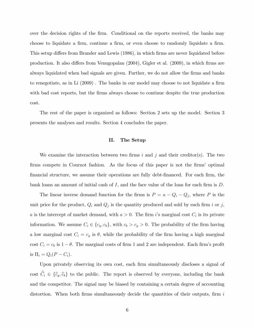
A. Unbiased system B. Conservative system C. Agressive system

Figure 1. Illustration of different accounting systems

The accounting systems in our model can only bias accounting reports in one direction.

That is, the conservative system only generates downwardly biased report and the aggressive

system only generates upwardly biased report. The degree of bias is captured in the variables

γ and δ. Specifically, the lower γ the more conservative the conservative system is, and the

higher δ the more agressive the agressive system is. Note that the case of agressive accounting

systemis not a prevalent phenomenon in practice. We nevertheless examine it for the sake

of completeness. The posterior probabilities under the three accounting systems are defined

as:

Unbiased System: α = 1 β = 1

Conservative System: α = 1 β = 1−θ(1−θ)+θ(1−γ)

Aggressive System: α = θθ+((1−θ)δ) β = 1

The sequence of the game is as follows. At time 0, the firms borrow the needed cash

from the bank(s). At time 1, nature reveals the firms’marginal costs, which can only be

observed by the firms themselves. Each firm discloses a public signal that is generated by

the firm’s accounting system. The signal is observed by both the bank and the competitor.

The firm’s decision rights are controlled by the firm if the reported signal is good, and by the

bank if the reported signal is bad. At time 2, the bank makes its decision to either continue

or terminate the firm’s operations. Thus at time 3, there are three possible outcomes. If

8

both firms are terminated, then there is no market. If only one firm survive, it becomes a

monopoly. If both firms survives, there is Cournot competition. At time 4, the firms make

respective quantity decisions. At last, payoffs are then realized for all parties involved at the

end.

In the next sections, we analyze the role of the accounting system in several variations

of the model described above. To establish a baseline, we first examine the impact of the

accounting systems on firms’ payoffs in a debt-free environment. Then we examine the

accounting effect when two firms each borrow debt from two independent banks. The third

case we investigate is when the two competing firms borrow from the same bank. In each

of these cases, we contrast the results from an unbiased accounting system with that from a

conservative system and an aggressive accounting system.

III. Equity Financing

We first examine the case when firms are fully equity-financed. Since there is no debt,

there is no need for the bank. As described above, the two firms have the same binary cost

realization. They then provide cost reports to the public. Finally the two firms compete

based on the information they have.

A. Unbiased Accounting System

Suppose the firms’true costs have to be reported without any bias. That is, a good

cost is reported as good with 100 percent probability, and a bad cost is reported as bad with

100 percent probability. It is in effect equivalent to firms’true costs being public knowledge.

Since there is no imperfect information, we simply denote the firm profit as a function of its

own cost and the competitor’s cost. For example, Π (cg,cg) refers to firm profit when its own

cost and its competitor’s cost are both good. There are four possible levels of profit for firm

i:

1. With probability θ2, both firms have good cost realizations, and the firm profit from

9

Cournot competition is Π (cg,cg) = (a−cg)2

9.

2. With probability (1− θ)2 , both firms have bad cost realizations, and the firm profit

from Cournot competition is Π (cb,cb) = (a−cb)29

.

3. With probability θ (1− θ) , firm i’s own cost is good and the competitor’s cost is bad,

and firm profit is Π (cg,cb) = ((a−cg)+(cb−cg))2

9.

4. With probability θ (1− θ) , firm i’s own cost is bad and the competitor’s cost is good,

and firm profit is Π (cb,cg) = ((a−cb)−(cb−cg))2

9.

The total expected profit E (Πunb.) for firm i is simply the weighted average of the above

values.6

B. Conservative Accounting System

Now we examine the case when the two competing firms are subject to an accounting

system with conservative bias. Under conservative accounting system, the firms must report

bad cost when the true cost is bad. But when the true cost is good, the firm may report

good cost with probability γ and report good cost with probability 1− γ. A firm’s profit is

a function of its own cost, its reported cost and its competitor’s reported cost. We denote

a firm’s profit and production quantity accordingly. For example, Π (cg,cg,cg) refers to the

firm profit when its cost is good, its reported signal is good, and its competitor’s reported

cost is good.

With conservatively-biased accounting signal, there are 6 possible levels of firm profit:

1. With probability θ2γ2, firm i has good cost, reports good cost and its competitor also

reports good cost. The firm’s profit is Π (cg,cg,cg) = (a−cg)2

9. This profit is the same as

that under the unbiased accounting system when both firms have good costs. This is

6Note the total expected production quantities when there is perfect information and when there issymmetric imperfect information (when firms do not even know their own cost realization) are the same,but the total expected firm profits is higher when there is perfect information.

10

because good signal is fully informative under conservative accounting system. Thus

when both firms send out good cost signals, they both know their competitors’costs

are truly good.

2. With probability θ2γ(1− γ), firm i has good cost, reports bad cost and its competitor

reports good cost. The firm’s profit is then Π (cg,cb,cg) = (2(a−cg)−β(cb−cg))2

36, with β =

1−θ(1−θ)+θ(1−γ)

.

3. With probability θγ(1 − θ), firm i has bad cost, reports bad cost and its competitor

reports good cost. The firm’s profit is then Π (cb,cb,cg) = (2(a−cb)−(1+β)(cb−cg))2

36.

4. With probability θγ (1− θγ), firm i has good cost, reports good cost and its competitor

reports bad cost. The firm’s profit is then Π (cg,cg,cb) = (2(a−cg)+2β(cb−cg))2

36.

5. With probability θ(1 − γ) (1− θγ), firm i has good cost, reports bad cost and its

competitor reports bad cost. The firm’s profit is then Π (cg,cb,cb) = (2(a−cg)+β(cb−cg))2

36.

6. With probability (1− θ) (1− θγ), firm i has bad cost, reports bad cost and its com-

petitor reports bad cost. The firm’s profit is then Π (cb,cb,cb) = (2(a−cb)−(1−β)(cb−cg))2

36.

The expected firm profit E (Πcon.)is the weighted-average of above firm profits.

C. Agressive Accounting System

Under an aggressive accounting system, the firms must report good cost when the true

cost is good. But when the true cost is bad, the firm may report bad cost with probability

δ and report good cost with probability 1− δ. There are also 6 possible levels of firm profit:

1. With probability θ (θ + δ − θδ), firm i has good cost, reports good cost and its com-

petitor also reports good cost. The firm’s profit is Π (cg,cg,cg) = (2(a−cg)+(1−α)(cb−cg))2

36b,

with α = θθ+((1−θ)δ) .

11

2. With probability θ(1− θ) (1− δ), firm i has good cost, reports good cost and its com-

petitor reports bad cost. The firm’s profit is then Π (cg,cg,cb) = (2(a−cg)+(1+α)(cb−cg))2

36b.

3. With probability δ (1− θ) (θ + δ − θδ), firm i has bad cost, reports good cost and its

competitor reports good cost. The firm’s profit is then Π (cb,cg,cg) = (2(a−cb)−α(cb−cg))2

36b.

4. With probability (1− θ)2 δ (1− δ), firm i has bad cost, reports good cost and its com-

petitor reports bad cost. The firm’s profit is then Π (cb,cg,cb) = (2(a−cb)+α(cb−cg))2

36b.

5. With probability (1− θ) (1− δ) (θ + δ − θδ), firm i has bad cost, reports bad cost and

its competitor reports good cost. The firm’s profit is thenΠ (cb,cb,cg) = (2(a−cb)−2α(cb−cg))2

36b.

6. With probability (1− θ)2 (1− δ)2, firm i has bad cost, reports bad cost and its com-

petitor reports bad cost. The firm’s profit is then Π (cb,cb,cb) = (a−cb)29b

.This profit is the

same as that under the unbiased accounting system when both firms have bad costs.

This is because bad signal is fully informative under aggressive accounting system.

Thus when both firms send out bad cost signals, they both know their competitors’

costs are truly bad.

Again, the total expected firm profit E(Πagg.) is just the weighted average of the values

outlined above.

By examining the firms’payoffs, it is obvious that the firms would always prefer to

report good signal even when its true cost is bad. Thus under aggressive accounting system,

the competing firms prefer to report aggressively.

Proposition 1. When firms compete in Cournot fashion in a debt-free world, their profits

under conservative/aggressive accounting systems are strictly lower than that under unbiased

accounting system, and their profits decreases with the level of conservatism/aggressiveness.

Proof. See appendix.

Proposition 1 demonstrates that accounting bias decreases the amount of firm profit

in a Cournot setting. The firms thus prefer a less biased accounting regime. The reason

12

for the decreased profit is the effi ciency loss caused by accounting distortion. Note there

are two scenarios when the firm profit is higher under conservative accounting system than

that under an unbiased accounting system: Π (cg,cg,cb) and Π (cg,cb,cb). However, the profits

from the other four scenarios are all lower than that under unbiased accounting system. The

losses thus outweigh the gains.

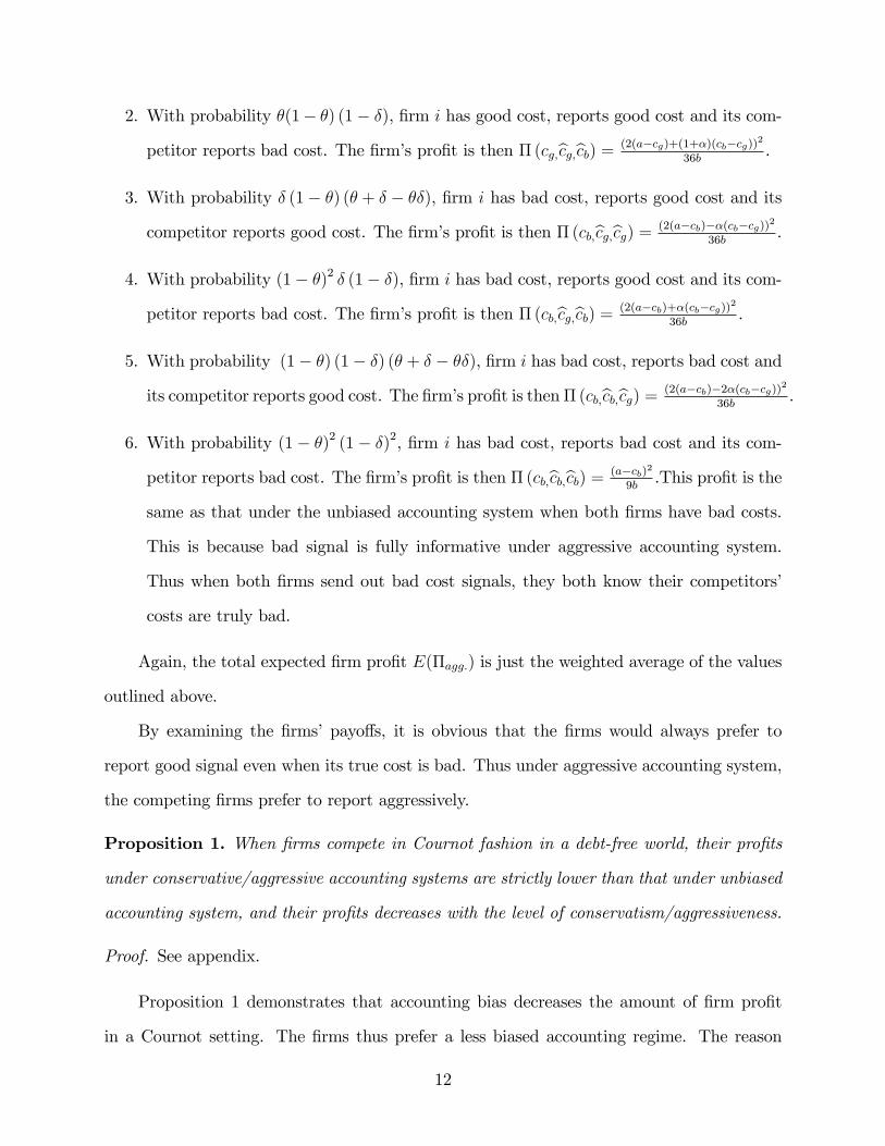
The following two figures visually demonstrate the effi ciency loss due to accounting

distortion.

0.0 0.2 0.4 0.6 0.8 1.0

7.40

7.45

7.50

7.55

7.60

7.65

gamma

firm profit

0.0 0.2 0.4 0.6 0.8 1.0

7.40

7.45

7.50

7.55

7.60

7.65

delta

firm profit

A: Conservative bias B: Aggressive bias

– unbiased system; - - - conservative system; · · · agressive system

Numerical values: θ=0.5, a=10, cg=1, cb=3.

Figure2: Firm profit level as a function of accounting bias.

IV. Debt Financing

Now we introduce debt into the model. We assume the two competing firms each must

finance their production through a different creditor. The probability distribution of cost is

ex-ante known to all the players of the game. At time 0, each of the two firms borrows debt

with face value D from its creditor. The cash flow paid out to each firm by the creditor is

I. The firms then disclose their costs generated by their reporting systems.

Absent renegotiation, it can be easily seen that the firm’s owner will always prefer to

13

continue the operations, since the payoff of termination is 0. However, the creditors will only

prefer to continue when the payoff of continuing is higher than liquidation value K, which

represents the depreciated firm assets at time 2. Note the creditors never have incentive to

discontinue the operations if K is suffi ciently small. Thus here we assume K is large enough

to guarantee a more interesting story involving possible liquidation. When a good signal

is reported, the firm’s decision rights reside with the firm’s owner who will continue the

firm’s operations. When a bad signal is reported, the firm’s decision rights transfer to the

creditor who may choose to liquidate. The payoffs for the banks and the borrowing firms are

determined at the end of the timeline. When a firm reports a good signal, and hence does

not violate the debt covenant, the bank gets min{D; Π} and the firm gets max{0,Π −D}.

When a firm reports bad signal and is terminated by the bank, the bank gets the liquidation

value K and the firm gets 0. When a firm reports bad signal but is allowed to continue by

the bank, the bank gets Π and the firm gets 0.

A. Unbiased Accounting System

We first examine the firm payoffs under an unbiased accounting system. We assume

the firms’liquidation value K is higher than the profit level of a firm with bad cost that

competes in the Cournot market. That is, K > Πc (cb, cb) > Πc (cb, cg). (The subscript "c"

denotes Cournot competition.) Thus the bank will always choose to discontinue the firm’s

operation whenever the firm’s reported cost is bad.

An interesting consequence emerges when one firm reports good signal and the other bad

signal. The firm with bad signal is liquidated, and the remaining firm becomes a monopolist,

with a profit even higher than when both firms have good cost. That is, Πm (cg) > Πc (cg,cg).

(Here the subscript "m" denotes monopoly market.) The payofftable for the banks and firms

14

is shown below:

Bank 1; 2

Firm 1; 2Prob. = θ Prob. = 1− θ

Prob. = θD;D

Πc (cg,cg)−D; Πc (cg,cg)−D

D;K

Πm (cg)−D; 0

Prob. = 1− θK;D

0; Πm (cg)−D

K;K

0; 0

Table 1. Payoffs of banks/firms under unbiased accounting system

Each bank’s expected payoff is

(2) θ2D + (1− θ)2K + θ(1− θ) (D +K) = K −Kθ + θD.

With the bank’s zero profit constraint, we know K −Kθ+ θD = I, and thus D = I−Kθ

+K.

Firm i’s expected payoff is

(3) θ2 (Πc (cg, cg)−D) + θ(1− θ) (Πm (cg)−D) ,

where Πc (cg, cg) = (a−cg)2

9and Πm (cg) = (a−cg)2

4. Thus, firm i’s expected profit is

E (Πunb.) = θ2

((a− cg)2

9−D

)+ θ(1− θ)

((a− cg)2

4−D

)

= θ2 (a− cg)2

9+ θ(1− θ)(a− cg)2

4− (I −K + θK)(4)

Bank’s Decision.– The bank has three possible decision choices when receiving a bad

cost report: to always continue, to always liquidate, or liquidate randomly. Obviously, if K

is lower than the firm’s profit level, then the bank would always choose to let the firm with

15

bad cost continue. In that case, the bank’s payoff would then be

(5) θ2D + (1− θ)2 Πc (cb,cb) + θ(1− θ) (D + Πc (cb,cg)) .

In the previous section, we assume the liquidation value K is strictly higher than the firm

profit level when its cost is bad. Thus the bank always liquidates a firm when the firm gives a

bad report. However, a complication arises when the cost reports sent out by both firms are

bad. If one bank chooses to let its borrowing firm continue, while the other bank liquidates

the other borrowing firm, the remaining firm would turn into a monopolist and generates

a profit Πm (cb) that could be higher than K. When Πm (cb) > K, the banks could use a

random strategy in liquidating the borrowing firms and improve the payoffs for all players.

Lemma 2. Under an unbiased accounting system, when both firms report bad cost, and when

Πm (cb) > K, the banks may let their borrowing firms continue operating with probability

Πm(cb)−KΠm(cb)−Πc(cb,cb)

to improve the total welfare of all players.

Proof. See Appendix.

Lemma 2 demonstrates the flexibility a competitive product market provides to the

creditors of the firms competing in the market. Even when both firms are in bad condition,

the random termination of one firm softens competition, thus give the remaining firm a

chance to be profitable again. The optimal probability of liquidation is simply the usual

ratio between the difference in payoffs induced by different decisions. Since the banks are

assumed to earn zero profit, any gain from the random liquidation would be transferred to

the borrowing firms in reduced interest rates. The random liquidation strategy thus provides

a Pareto improvement to the payoffs of all players.7

Note that the effect demonstrated in Lemma 2 is independent of potential accounting

7We do not consider the potential welfare impact to consumers created by the change in product marketstructure. It is not immediately clear whether the consumer surplus would increase or decrease. For example,the random liquidation strategy could potentially improve consumer welfare since it prevents a completemarket shutdown.

16

influence, as there is no bias under unbiased accounting system. We show in the following

section this effect could be amplified when the accounting system is biased. Also note the

increase in number of firms in Cournot competition does not change the qualitative nature

of the result. For simplicity, we include two competing firms in our model. As the number of

firms competing in the same product market increases, the competition becomes more fierce.

Nevertheless, the liquidation of one firm still softens the market competition and leaves the

surviving firms better off.

B. Conservative Accounting System

Now we switch to the conservative accounting system. Following the same setup as

under the unbiased accounting system, we first assume banks always liquidate the firms with

a bad cost report. Thus, firms that have good cost but report bad cost under the conservative

17

accounting system would also be liquidated.

Bank 1

Bank 2Prob. = θγ Prob. = θ(1− γ) Prob. = (1− θ)

Firm 1

Firm 2

Prob. = θγ

D

D

Πc (cg,cg)−D

Πc (cg,cg)−D

K

D

0

Πm (cg)−D

K

D

0

Πm (cg)−D

Prob. = θ(1− γ)

D

K

Πm (cg)−D

0

K

K

0

0

K

K

0

0

Prob. = (1− θ)

D

K

Πm (cg)−D

0

K

K

0

0

K

K

0

0

Table 2. Payoffs of banks/firms under conservative accounting system.

Examining the payoff table, we can see the conservative accounting system induces inappro-

priate termination of firms with good cost. The total expected payoff to the bank is the

weighted average of above values:

(6) θγD + (1− θγ)K

This payoff is lower than the bank payoff under the unbiased accounting system of

18

θD + (1− θ)K. With the bank facing the same zero profit constraint, we have

(7) D =I −K + θγK

θγ.

Firm i’s expected profit is

(8) E(Πcon.) = θ2γ2 (a− cg)2

9+ θγ (1− θγ)

(a− cg)2

4− (I −K + θγK) .

Interestingly, under certain circumstances, the firms’expected profits under the conser-

vative accounting system could even be higher than that under unbiased accounting system.

Proposition 3. When (θ + θγ)(

(a−cg)2

4− (a−cg)2

9

)>(

(a−cg)2

4−K

), and θ 6= 0, γ 6= 1, the

firms’expected profits are higher under the conservative accounting system than that under

the unbiased accounting system.

Proof. See Appendix.

The above proposition demonstrates that accounting conservative bias induces two ef-

fects in the expected profits of the Cournot firms. One effect is the increased likelihood

of a firm becoming a monopolist (as shown in Lemma 2). The second effect is the de-

creased chance of survival due to the creditors’excessive liquidation. When the first effect

dominates the second, the firms’ expected profits actually increase when there is an im-

posed conservative bias. Note that the second effect reduces the firm profit by the amount

θ (1− γ) (Πm (cg)−K). This is because when a firm is liquidated, the creditor still gets

liquidation value K. Since the creditors face zero-profit constraint, any extra value it gains

will be still passed back to the firms through lower interest payments.

In addition, the firm’s profit under the conservative accounting system depends on some

parameter values.

Corollary 4. Under the conservative accounting system, the firms’profits decrease with the

19

degree of accounting conservatism when Πm (cg) − K > 2θγ (Πc (cg,cg)− Πm (cg)); and in-

crease with the degree of accounting conservatism when Πm (cg)−K > 2θγ (Πd (cg,cg)− Πm (cg)).

Proof. See Appendix.

The intuition behind the corollary 4 comes from the debts’role in changing the compet-

itive nature of the industry. Although a conservative accounting system imposes excessive

liquidation on firms that report a bad cost signal, it turns the surviving firm into a monopo-

list that generates higher profit than a Cournot duopolist. When the difference between the

monopolist profit and duopolist profit is higher than the difference between the monopolist

profit and the liquidation value, higher degree of conservatism actually increases firm profit.

Combining the findings of Proposition 3 and Corollary 4, we know that the firms’

profits under the conservative accounting system could be higher than that under the un-

biased accounting system when (Πm (cg)−K) < (θ + θγ) (Πm (cg)− Πc (cg,cg)) . Further,

the firm profits increase as the degree of conservatism increases when Πm (cg) − K <

2θγ (Πm (cg)− Πc (cg,cg)) .This result is quite different from the prior literature on the effect

of debt on conservatism, which typically shows conservatism decreases debt effi ciency. The

reason for the different result in our setting is due to the fact that accounting conservatism

can indirectly change the industry structure through the firms’debt contracts.

Banks’Liquidation Decision.– Now we examine the creditors’decision to liquidate

versus to let continue a firm that reports a bad signal. As under the unbiased accounting

system, the liquidation decision largely depends on the value of K. If the banks never

liquidate the firms with bad cost signals, the bank’s payoff is

θγD + θ2γ(1− γ)Πc (cg,cb,cg) + θ(1− γ) (1− θγ) Πc (cg,cb,cb)

+θγ (1− θ) Πc (cb,cb,cg) + (1− θ) (1− θγ) Πc (cb,cb,cb) .(9)

Hence, the necessary condition for the bank to choose to always continue a firm with a

20

bad cost signal is for the bank’s payoff to be higher if this firm is continued. That is,

θ2γ(1− γ)Πc (cg,cb,cg) + θ(1− γ) (1− θγ) Πc (cg,cb,cb)

+θγ (1− θ) Πc (cb,cb,cg) + (1− θ) (1− θγ) Πc (cb,cb,cb)(10)

> (1− θγ)K

Obviously, the smaller the liquidation value K is, the more likely it is the above inequal-

ity will hold. Conversely, when the bank knows the cost report issued by the firm it lends to

is bad, and the cost report the rival firm sends out is good, the bank should always liquidate

the firm if (1− β) Πc (cg,cb,cg) + βΠc (cb,cb,cg) < K.

Similar to Lemma 2, the bank could use a random strategy in the liquidation decision

if Πm (cb) > K, when the cost reports sent out by both firms are bad.

Corollary 5. Under the conservative accounting system,when both firms report bad cost, and

when Πm (cb) > K, the banks let their borrowing firms continue operating with probability

βΠm(cb)+(1−β)Πm(cg)−KβΠm(cb)+(1−β)Πm(cg)−βΠc(cb,cb,cb)+(1−β)Πc(cg,cb,cb)

to improve the total welfare of all players.

Proof. See Appendix.

The intuition of corollary 5 is similar to that of Lemma 2, except that the conservative

bias in the accounting system effectively increases the decision space for the banks. The banks

hence have more flexibility in their liquidation decisions to improve the players’payoffs.

C. Aggressive accounting system

Now we analyze when there is an aggressive accounting distortion in the firms’reports.

Contrary to the conservative system, the firms must report good cost as good cost, and may

report good or bad when the cost is truly bad. Again we first examine the payoff table of

21

the banks and firms.

Bank 1

Bank 2Prob. = θ

Prob. =

(1− θ) δ

Prob. =

(1− θ) (1− δ)

Firm 1

Firm 2

Prob. = θ

D

D

Πc (cg,cg, cg)−D

Πc (cg,cg, cg)−D

Πc(cb,cg, cg)

D

0

Πc (cg,cg, cb)−D

K

D

0

Πm (cg)−D

Prob. =

(1− θ) δ

D

Πc(cb,cg, cg)

Πc (cg,cg, cb)−D

0

Πc (cb,cg, cb)

Πc (cb,cg, cb)

0

0

K

D

0

Πm (cb)−D

Prob. =

(1− θ) (1− δ)

D

K

Πm (cg)−D

0

D

K

Πm (cb)−D

0

K

K

0

0

Table 3. Payoffs of banks and firms under aggressive accounting system

Examining the payoff table, it is clear the problem under aggressive accounting system

is the inappropriate continuation of firms with bad costs. The total expected payoff to the

bank is:

(θ + (1− θ)2 δ (1− δ)

)D + θ (1− θ) δΠc(cb,cg, cg)

+ (1− θ)2 δ2Πc(cb,cg, cb) + (1− θ) (1− δ)K(11)

22

Again, the banks’payoffs are smaller compared to the banks’payoffs under the unbiased

accounting system of θD + (1− θ)K, since Πc(cb,cg, cg) < K and Πc(cb,cg, cb) < K. With

the bank facing the same zero profit constraint, we set the bank’s payoff equal to I and have

(12) D =

(I − θ (1− θ) δΠc(cb,cg, cg)− (1− θ)2 δ2Πc(cb,cg, cb)− (1− θ) (1− δ)K

)(θ + (1− θ)2 δ (1− δ)

) ,

then we have firm i’s expected profit

E (Πagg.) = θ2

(2 (a− cg) + (1− θ

θ+((1−θ)δ)) (cb − cg))2

36

+θ (1− θ) δ

(2 (a− cg) +

(1 + θ

θ+((1−θ)δ)

)(cb − cg)

)2

36b(13)

+θ (1− θ) (1− δ) (a− cg)2

4+ (1− θ) δ (1− δ) (a− cb)2

4

−

I − θ (1− θ) δ (2(a−cb)− θθ+((1−θ)δ) (cb−cg))

2

36b

− (1− θ)2 δ2 (2(a−cb)+ θθ+((1−θ)δ) (cb−cg))

2

36b− (1− θ) (1− δ)K

Compared to the firm’s payoff under the unbiased accounting system, the firm’s payoff

is almost always lower, except that Πc (cg,cg, cg) > Πc (cg, cg) with probability θ2.8

Proposition 6. When θ2 (Πc (cg,cg, cg)− Πc (cg, cg)) > (θ(1− θ)Πm (cg)− (I −K + θK))− θ (1− θ) δΠc (cg,cg, cb) + θ (1− θ) (1− δ) Πm (cg) + (1− θ) δ (1− δ) Πm (cb)

−(I − θ (1− θ) δΠc(cb,cg, cg)− (1− θ)2 δ2Πc(cb,cg, cb)− (1− θ) (1− δ)K

), and θ 6=

0, δ 6= 1, the firms’expected profits are higher under aggressive accounting system than that

under unbiased accounting system.

Proof. The result is immediately clear from examining the expected firm profit levels under

unbiased and aggressive accounting systems.

8The profit levels of firms with good costs competing under the agressive accounting system is higherthan under unbiased accounting system. The reason is that under an agressive accounting system, the firmstake into consideration that the rivals’reported good cost may not be true. The competition is thus softenedas both firms lower their production quantities accordingly.

23

The above proposition shows that only when θ is suffi ciently large is it possible for

an aggressive accounting system to induce higher profit for the firms than under unbiased

system.

Banks’decision.–Without renegotiation, the banks have no way to prevent the prob-

lem of inappropriate continuation of firms with bad costs. The managers of the borrowing

firms, on the other hand, have no incentive to terminate the firms by themselves. Thus there

is no possible correction to the error induced by the aggressive accounting system.

V. One Bank and Two Firms

Now we introduce another scenario where the competing firms borrow from the same

creditor. The change from two creditors to one common creditor is non-trivial. The firms’

cost realizations are independent of each other, and the common creditor in our model still

cannot infer one firm’s cost from the other. However, now the single creditor is able to

manipulate the competitive nature of the market by strategic liquidation. The payoffs with

one creditor are mostly the same as when there are two banks lending to two firms, but the

bank maximizes its payoff from the whole industry rather than from each individual firm.

Therefore, when both firms report bad cost signals, the bank may be better off letting one

firm survive. Especially, when the profit of a monopolist with bad cost Πm (cb) > K, the

strategic liquidation provides a Pareto improvement on all players’payoffs.

A. Unbiased accounting system

We again first examine the payoffs under the unbiased accounting system. The payoff

to the bank is essentially the sum of the two banks in the previous analyses. Examining

the lower right cell of Table 1, in which both firms report bad cost signals, the best the two

banks can do is to use random strategy to liquidate the firms (as described in Lemma 1).

However, when there is one bank lending to both firms, it is able to deterministically let one

24

firm liquidate and the other continue as a monopolist. Its payoff is thus:

(14) θ22D + (1− θ)2 (K + Πm (cb)) + 2θ(1− θ) (D +K) .

Since the above must equal the total initial cash investment 2I, we know

(15) D =2I − (1− θ)2 Πm (cb)− (1− θ)(1 + θ)K

2θ,

which is strictly lower than I−(1−θ)Kθ

if the bank does not perform such random liquidation.

Since the bank faces zero-profit constraint, all the extra profit is transferred to the firms

through lower interest rate. Firm i’s payoff is

θ2 (Πd (cg, cg)−D) + θ(1− θ) (Πm (cg)−D)(16)

= θ2Πd (cg, cg) + θ(1− θ)Πm (cg)−2I − (1− θ)2 Πm (cb)− (1− θ)(1 + θ)K

2,

which is strictly higher than θ2Πd (cg, cg)+θ(1−θ)Πm (cg)−(I −K +Kθ) , the payoff should

such random liquidation not occur.

B. Conservative accounting system

Compared to the unbiased accounting system, the probability of both firms reporting

a bad cost is higher under the conservative accounting system. In fact, the four lower

right cells in Table 2 all contain double liquidations. With one bank lending to both firms,

one liquidation and one monopolist survivor would replace these cells instead. The bank’s

expected payoff would then be:

(17) 2θγD + 2θγ (1− θγ)K + θ (1− γ) (1− θγ) Πm (cg) + (1− θ) (1− θγ) Πm (cb)

This payoff is greater than the bank payoff under strategic random liquidation. Again

25

we compute the face value of the debt:

(18) D =2I − 2θγ (1− θγ)K − θ (1− γ) (1− θγ) Πm (cg)− (1− θ) (1− θγ) Πm (cb)

2θγ,

which is smaller than if the bank does not perform the random liquidation.

The firm i’s expected profit is thus

θ2γ2Πc (cg,cg) + θγ (1− θγ) Πm (cg)−(19)

2I − 2θγ (1− θγ)K − θ (1− γ) (1− θγ) Πm (cg)− (1− θ) (1− θγ) Πm (cb)

2

C. Aggressive Accounting System

As shown in Table 3, the aggressive accounting system also has one cell where both

firms are liquidated. The single bank that lends to both firms could also replicate the same

strategy to liquidate one firm and turn the surviving rival into a monopolist. However,

the probability of both firms report bad cost is much smaller than that under conservative

system.

The results of above finding is summarized in the following proposition.

Proposition 7. Under all accounting systems, when two competing firms borrow from one

common bank, the bank may improve the overall payoffs by turning one of the two firms that

report a bad cost into a surviving monopolist.

Proof. The result is immediately clear from examining the banks/firms payoffs.

VI. Conclusion

We show accounting biases decrease the expected firm profits when the firms compete in

Cournot product market in a debt-free world. However, some different results emerge when

debt is introduced into the firms’financial structure. Specifically, when accounting reports

are used for debt covenants, accounting biases affect the likelihood of covenant violation

26

and the banks’subsequent liquidation decision. When one of the two firms is terminated,

the other one becomes a monopolist. The surviving firm is then able to capture the entire

market share,making a profit higher than when it competes with a rival firm. We then

demonstrate the firms’payoffs under the conservative accounting system could be higher

than that under the unbiased accounting system. In addition, the conservative accounting

system provides the creditors with more control by triggering debt covenant violation more

frequently. The creditors can reduce "false positives" by not always terminating firms with

bad reports. Further, the creditors can choose to randomly allow one firm to survive when

both firms report bad signals. The remaining monopolist then generates enough profit to

pay back the debt. With assumption of zero-profit constraint for the bank, the extra gain

from conservative accounting is passed to the firms through decreased interest rates.

Our study shows accounting bias could have a real effect on the firms’operating de-

cisions through the presence of debt. Accounting is often perceived to be just a distortion

of information, and not have real impact on the economic agents’behavior. However, the

accounting bias in our setting could change the competitive nature of market in which the

borrowing firms compete.

REFERENCES

Athey, S., and K. Bagwell. 2001. Optimal collusion with private information. RAND Journal

of Economics, 32 (3), 428-465.

Bagwell, K., 1995. Commitment and observability in games. Games and Economic Behavior,

8 (2), 271-280.

Bagnoli, M., and S.G. Watts, 2010. Oligopoly, disclosure, and earnings management. The

Accounting Review, 85 (June).

Basu, S., 1997. The conservatism principle and the asymmetric timeliness of earnings. Journal

of Accounting and Economics, 24, 3-37.

27

Beatty, A., J. Webber and J. Yu, 2008. Conservatism and debt. Journal of Accounting and

Economics, 45 (2-3), 157-174.

Brander, J.A., and T.R. Lewis, 1986. Oligopoly and financial structure: The limited liability

effect. The American Economic Review, 76 (5), 956-970.

Corona, C., and Nan, L., 2010. Bluffi ng contests: The real effects of pre-announcing com-

petitive decisions. Working paper, Carnegie-Mellon University

Clayton, M. J. and B. Jorgensen 2005, Optimal Cross Holding with Externalities and Strate-

gic Interactions. Journal of Business, Vol. 78, No. 4, July, pp. 1505 —1522.

Demerjian, P., 2011. Accounting Standards and Debt Covenants: Has the “Balance Sheet

Approach”Led to a Decline in the Use of Balance Sheet Covenants?”Journal of Accounting

and Economics, forthcoming.

Darrough, M., 1993. Disclosure bolicy and competition: Cournot vs. Bertrand. The Account-

ing Review, 68 (3), 534—561.

Darrough, M. N. and NM. Stoughton. Financial Disclosure Policy in an Entry Game. Journal

of Accounting and Economics 12 (1990), 219-243

Gigler, F., C. Kanodia, H. Sapra and R. Venugopalan, 2009. Accounting conservatism and

the effciency of debt contracts. Journal of Accounting Research 47 (3), 767-797.

Hughes, J.S., J. Kao, and A. Mukherji, 1998. Oligopoly, financial structure, and resolution

of uncertainty. Journal of economics and Management Strategy, 7 (1), 67-88.

Hughes, J.S., and M.G. Williams, 2008. Commitment and disclosure in oligopolies. The

Accounting Review, 83 (1).

Li, J. 2009. Accounting Conservatism and Debt Contracts: Effi cient Liquidation and

Covenant Renegotiation. Working paper, Carnegie-Mellon University

28

Venugopalan, R., 2004. Conservatism in accounting: good or bad? Working paper, University

of Chicago.

Watts, R.L., 2003. Conservatism in accounting Part I: Explanations and implications. Ac-

counting Horizons, 3, 207-221.

Appendix

A Computation of the firm profits in the debt-free world

To compute the expected firm profit, we must compute the firm profits for each of the

six scenarios under both conservative and aggressive systems.

A. With Conservative Bias

Scenario 1: When both firms report good signals.–When firm i has good cost,

reports good cost and its competitor firm j also reports good cost, we know both firms must

be reporting truthfully, since α = 1. That is, both firms must have the same true cost

and same reported cost. Thus the problem reduces to a standard Cournot game. Firm i’

objective function is:

(A1) qi (cg,cg,cg) (a− qi (cg,cg,cg)− qj (cg,cg,cg)− cg) .

Firm j’objective function is:

(A2) qj (cg,cg,cg) (a− qj (cg,cg,cg)− qi (cg,cg,cg)− cg) .

Both firms maximize their profit functions over q. Setting the two FOCs equal to zero

and solve for qi and qj , we have:

(A3) qi (cg,cg,cg) = qj (cg,cg,cg) =a− cg

3.

29

Substitute into the profit function, we have:

(A4) Πc (cg,cg,cg) =(a− cg)2

9.

Scenarios 2, 3 and 4: When one firm reports good signal and one firm reports

bad signal.– Suppose firm i reports a good signal and firm j reports a bad signal. Firm i

must have true good cost. Firm j could have true bad cost or have good cost but report a

bad cost. The three FOCs are:

(A5) qj (cg,cb,cg) =a− cg − qi (cg,cg,cb)

2

(A6) qj (cb,cb,cg) =a− cb − qi (cg,cg,cb)

2

(A7) qi (cg,cg,cb) =a− cg − (βqj (cb,cb,cg) + (1− β) qj (cg,cb,cg))

2

Solving for the three unknowns and applying symmetry, we have:

(A8) q (cg,cg,cb) =2 (a− cg) + 2β (cb − cg)

6

(A9) q (cg,cb,cg) =2(a− cg)− β(cb − cg)

6

(A10) q (cb,cb,cg) =2 (a− cb)− (1 + β) (cb − cg)

6

30

The corresponding firm profits are:

(A11) Π (cg,cg,cb) =(2 (a− cg) + 2β (cb − cg))2

36

(A12) Π (cg,cb,cg) =(2(a− cg)− β(cb − cg))2

36

(A13) Π (cb,cb,cg) =(2 (a− cb)− (1 + β) (cb − cg))2

36

Scenarios 5 and 6: When both firms report bad signals.–When two bad signals

are reported, the competing firms have symmetric imperfect information. Each firm must

take into consideration that the competitor could have truly bad cost, or have good cost

but report bad. Firm i maximizes its profit by choosing production quantity qi so that

∂∂qi

(qi(a− qi − E (qj)− ci) = 0, where E(qj) = βqj (cb,cb,cb) + (1− β) qj (cg,cb,cb). Firm j

does the same. Applying symmetry, we have the following four equations:

(A14) qi (cb,cb,cb) =1

2(a− cb − βqj (cb,cb,cb)− (1− β) qj (cg,cb,cb))

(A15) qi (cg,cb,cb) =1

2(a− cg − βqj (cb,cb,cb)− (1− β) qj (cg,cb,cb))

(A16) qj (cb,cb,cb) =1

2(a− cb − βqi (cb,cb,cb)− (1− β) qi (cg,cb,cb))

(A17) qj (cg,cb,cb) =1

2(a− cg − βqi (cb,cb,cb)− (1− β) qi (cg,cb,cb))

31

Solving the four equations and applying symmetry, we have:

(A18) q (cg,cb,cb) =2 (a− cg) + β(cb − cg)

6

(A19) q (cb,cb,cb) =2 (a− cb)− (1− β) (cb − cg)

6

Firm i’s profit is:

(A20) Π (cg,cb,cb) =(2(a− cg) + β (cb − cg))2

36

(A21) Π (cb,cb,cb) =(2(a− cb)− (1− β) (cb − cg))2

36

B. With Aggressive Bias

Scenarios 1 and 2: when both firms report good signals.–When two good

signals are reported, the firms could have truly good cost, or have bad cost but report good.

Thus, firm i’s objective function is qi(a − qi − E (qj) − ci, where E(qj) = αqj (cg,cg,cg) +

(1− α) qj (cb,cg,cg). Firm j does the same. Applying symmetry, we have 4 equations:

(A22) qi (cg,cg,cg) =1

2(a− cg − αqj (cg,cg,cg)− (1− α) qj (cb,cg,cg))

(A23) qi (cb,cg,cg) =1

2(a− cb − αqj (cg,cg,cg)− (1− α) qj (cb,cg,cg))

(A24) qj (cg,cg,cg) =1

2(a− cg − αqi (cg,cg,cg)− (1− α) qi (cb,cg,cg))

32

(A25) qj (cb,cg,cg) =1

2(a− cb − αqi (cg,cg,cg)− (1− α) qi (cb,cg,cg))

Solving the four equations and applying symmetry, we have:

(A26) q (cg,cg,cg) =2 (a− cg) + (1− α) (cb − cg)

6

(A27) q (cb,cg,cg) =2 (a− cb)− α (cb − cg)

6

Firm i’s profit is:

(A28) Π (cg,cg,cg) =(2 (a− cg) + (1− α) (cb − cg))2

36

(A29) Π (cb,cg,cg) =(2 (a− cb)− α (cb − cg))2

36

Scenarios 3, 4 and 5: When one firm reports a good signal and one firm

reports a bad signal.– Let firm i report a good signal and firm j report a bad signal.

Firm i could have true good cost or have bad cost but report good cost. Firm j must have

true bad cost. The three FOCs are:

(A30) qi (cg,cg,cb) =a− cg − qj (cb,cb,cg)

2

(A31) qi (cb,cg,cb) =a− cb − qj (cb,cb,cg)

2

(A32) qj (cb,cb,cg) =a− cg − (αqi (cg,cg,cb) + (1− α) qi (cb,cg,cb))

2

33

Solving for the three unknowns and applying symmetry, we have:

(A33) q (cg,cg,cb) =2 (a− cg) + (1 + α) (cb − cg)

6

(A34) q (cb,cg,cb) =2(a− cb) + α(cb − cg)

6

(A35) q (cb,cb,cg) =2 (a− cb)− 2α (cb − cg)

6

And the corresponding firm profits are:

(A36) Π (cg,cg,cb) =(2 (a− cg) + (1 + α) (cb − cg))2

36

(A37) Π (cb,cg,cb) =(2(a− cb) + α(cb − cg))2

36

(A38) Π (cb,cb,cg) =(2 (a− cb)− 2α (cb − cg))2

36

Scenario 6: When both firms report bad signals.– Under aggressive accounting

system, the firms must have truly bad cost when they both report bad signals. Thus again

the problem reduces to a standard Cournot game. Firm i’s FOC is:

(A39) qi (cb,cb,cb) = qj (cb,cb,cb) =a− cb

3.

Substituting into the profit function, we have:

(A40) Π (cb,cb,cb) =(a− cb)2

9.

34

B Proof of Proposition 1

The expected payoffs of firm i in three different accounting systems are listed below.

Unbiased system:

E(Πunb.) = θ2 (a− cg)2

9+ (1− θ)2 (a− cb)2

9(B1)

+θ(1− θ)((a− cg) + (cb − cg))2

9+ (1− θ)θ ((a− cb)− (cb − cg))2

9

Conservative system:

E(Πcon.) = θ2γ2 (a− cg)2

9+ θγθ(1− γ)

(2(a− cg)− 1−θ

(1−θ)+θ(1−γ)(cb − cg)

)2

36

+θγ (θ(1− γ) + (1− θ))

(2 (a− cg) + 2 1−θ

(1−θ)+θ(1−γ)(cb − cg)

)2

36

+θ(1− γ) (θ(1− γ) + (1− θ))

(2(a− cg) + 1−θ

(1−θ)+θ(1−γ)(cb − cg)

)2

36

+θγ (1− θ)

(2 (a− cb)−

(1 + 1−θ

(1−θ)+θ(1−γ)

)(cb − cg)

)2

36(B2)

+ (1− θ) (θ(1− γ) + (1− θ))

(2(a− cb)−

(1− 1−θ

(1−θ)+θ(1−γ)

)(cb − cg)

)2

36

35

Aggressive system:

E(Πagg.) =(θ2 + θ (1− θ) δ

) (2 (a− cg) + (1− θθ+((1−θ)δ)) (cb − cg)

)2

36

+θ (1− θ) (1− δ)

(2 (a− cg) +

(1 + θ

θ+((1−θ)δ)

)(cb − cg)

)2

36

+(θ(1− θ)δ + (1− θ)2 δ2

) (2 (a− cb)− θθ+((1−θ)δ) (cb − cg)

)2

36(B3)

+ (1− θ) δ (1− θ) (1− δ)

(2(a− cb) + θ

θ+((1−θ)δ)(cb − cg))2

36

+ (θ (1− θ) (1− δ) + (1− θ) δ (1− θ) (1− δ))

(2 (a− cb)− 2 θ

θ+((1−θ)δ) (cb − cg))2

36

+ (1− θ)2 (1− δ)2 (a− cb)2

9

To compute the difference in these profits, we subtract the conservative/aggressive profit

from the unbiased profit.

(B4) E(Πunb.)− E(Πcon.) =11

36θ (cb − cg)2 (1− θ) 1− γ

1− θγ > 0

(B5) E(Πunb.)− E(Πagg.) =11

36θδ (cb − cg)2 1− θ

θ + δ − θδ > 0

Thus we know the profit level under unbiased accounting system is always higher than

that under conservative/aggressive accounting system.

To demonstrate the relationship between the firm profit and the level of conserva-

tive/aggressive bias, we take the partial derivative of firm i’s profit w.r.t. γ and δ.

(B6)∂

∂γE(Πcon.) =

11

36θ (cb − cg)2 (θ − 1)2

(θγ − 1)2 > 0

36

(B7)∂

∂γE(Πagg.) =

11

36θ2 (cb − cg)2 θ − 1

(θ + δ − θδ)2 < 0

It is clear that the higher level of bias is, the lower the firm profit.

C Proof of Lemma 2

Suppose bank 1 let the borrowing firm continue with bad cost report with probability

x, and bank 2 does so with probability y. Then bank 1 should have the following program:

(C1) max xyΠc (cb,cb) + x (1− y) Πm (cb) + (1− x)K

Taking the first order condition, we have:

∂

∂x(xyΠc (cb,cb) + x (1− y) Πm (cb) + (1− x)K)(C2)

= Πm (cb)−K + yΠc (cb, cb)− yΠm (cb) = 0

Solving for y, we have:

(C3) y =Πm (cb)−K

Πm (cb)− Πc (cb, cb).

D Proof of Proposition 3

The firms’expected profits under unbiased accounting system are

(D1) θ2Πc (cg,cg) + θ(1− θ)Πm (cg)− (I −K + θK) .

The firms’expected profits under conservative accounting system are

(D2) θ2γ2Πc (cg,cg) + θγ (1− θγ) Πm (cg)− (I −K + θγK) .

37

Taking the difference between these two expected profits, we have

θ2γ2Πc (cg,cg) + θγ (1− θγ) Πm (cg)− (I −K + θγK)

−(θ2Πc (cg,cg) + θ(1− θ)Πm (cg)− (I −K + θK)

)(D3)

= θ (1− γ) ((θ + θγ) (Πm (cg)− Πc (cg,cg))− (Πm (cg)−K)) .

We know Πm (cg) = (a−cg)2

4> Πc (cg,cg) = (a−cg)2

9> K. Thus the above value will be strictly

positive when (θ + θγ) (Πm (cg)− Πc (cg,cg)) > (Πm (cg)−K).

E Proof of Corollary 4

We examine the change of the firm’s profit in γ. Taking the partial derivative, we have

∂

∂γ

(θ2γ2Πc (cg,cg) + θγ (1− θγ) Πm (cg)− (I −K + θγK)

)(E1)

= θ ((Πm (cg)−K) + 2θγ (Πc (cg,cg)− Πm (cg))) .

Clearly the firms’profits will increase in γ if Πm (cg)−K > 2θγ (Πm (cg)− Πc (cg,cg)), which

means less conservatism leads to higher profit. However, ifΠm (cg)−K < 2θγ (Πm (cg)− Πc (cg,cg)),

the firms’profits will decrease in γ, which means higher conservatism leads to higher profit.

F Proof of Corollary 5

Suppose the bank let the borrowing firm continue with probability x. Then it will have

the following program:

maxx

xy (βΠc (cb,cb,cb) + (1− β) Πc (cg,cb,cb))(F1)

+x (1− y) (βΠm (cb) + (1− β) Πm (cg)) + (1− x)K

38

Setting the FOC = 0 and solving for y, we obtain

(F2) y =βΠm (cb) + (1− β) Πm (cg)−K

βΠm (cb) + (1− β) Πm (cg)− βΠc (cb,cb,cb) + (1− β) Πc (cg,cb,cb).

39