Fireball Models for Flares in AE Aquarii

Mon. Not. R. Astron. Soc. 000, 000–000 (2002)

Fireball Models for Flares in AE Aquarii

K. J. Pearson?†, Keith Horne, Warren Skidmore‡School of Physics and Astronomy, University of St. Andrews, North Haugh, St Andrews KY16 9SS

Accepted . Received ; in original form

ABSTRACT

We examine the flaring behaviour of the cataclysmic variable AE Aqr in the contextof the ‘magnetic propeller’ model for this system. The flares are thought to arise fromcollisions between high density regions in the material expelled from the system afterinteraction with the rapidly rotating magnetosphere of the white dwarf. We calculatethe first quantitative models for the flaring and calculate the time-dependent emergentoptical spectra from the resulting hot, expanding ball of gas. We compare the resultsunder different assumptions to observations and derive values for the mass, lengthscaleand temperature of the material involved in the flare. We see that the fits suggest thatthe secondary star in this system has Population II composition.

Key words: accretion, radiative transfer, stars: flares, stars: individual: AE Aqr,novae, cataclysmic variables

1 INTRODUCTION

AE Aqr is an unusual cataclysmic variable star exhibitingbizarre phenomena that can now be interpreted in the con-text of a magnetic propeller that throws gas out of the bi-nary system (Wynn, King & Horne 1997). The magneticpropeller efficiently extracts energy and angular momentumfrom the white dwarf and transports it via magnetic fieldsto gas stream material which it ejects from the binary sys-tem. Detailed understanding of the magnetic propeller ef-fects may therefore help us to unlock some of the secrets ofmagnetic viscosity in accretion flows.

In the AE Aqr binary system, a slightly evolved K star(Welsh, Horne & Gomer 1995) that overflows its Roche lobeis locked in a 9.88 hour orbit with a rapidly spinning magne-tized white dwarf. Coherent oscillations in optical (Patterson1979), ultraviolet (Eracleous et al. 1994), and X-ray (Patter-son et al. 1980) lightcurves reveal the white dwarf’s 33s spinperiod. The oscillation has two unequal peaks per spin cy-cle, consistent with broad hotspots on opposite sides of thewhite dwarf ∼ 15◦ above and below the equator (Eracleouset al. 1994). These oscillations are strongest in the ultravio-

? Send offprint requests to: [email protected]† Present address: Lousiana State University, Department ofPhysics and Astronomy, Nicholson Hall, Baton Rouge, LA 70803-4001, USA‡ Present address: Department of Physics and Astronomy, Uni-versity of California, Irvine, 4129 Frederick Reines Hall, Irvine,CA 92697-4575, USA

let, where their spectra show a blue continuum with broadLy α absorption consistent with a white dwarf (log g ≈ 8)atmosphere with T ∼ 3×104 K (Eracleous et al. 1994). Thesimplest interpretation is accretion heating near the poles ofa magnetic dipole field tipped almost perpendicular to therotation axis.

An 11-year study of the optical oscillation period (deJager 1994) shows that the white dwarf is spinning downat an alarming rate. Something extracts rotational energyfrom the white dwarf at a rate Iωω ∼ 60νLν ie. some 60times the luminosity of the system. We now believe that tobe a magnetic propeller. This model was first proposed byWynn, King & Horne (1995) and Eracleous & Horne (1996)and expanded upon in Wynn, King & Horne (1997) withcomparison of observed and modelled tomograms. Furtherwork on the flaring region was reported in Welsh, Horne &Gomer (1998) and Horne (1999).

The gas stream emerging from the companion starthrough the L1 nozzle encounters a rapidly spinning mag-netosphere. The rapid spin makes the effective ram pressureso high that only a low-density fringe of material becomesthreaded onto field lines. Most of the stream material re-mains diamagnetic, and is dragged toward co-rotation withthe magnetosphere. As this occurs outside the co-rotationradius, this magnetic drag propels material forward, boost-ing its velocity up to and beyond escape velocity. The ma-terial emerges from the magnetosphere and sails out of thebinary system. This process efficiently extracts energy andangular momentum from the white dwarf, transferring it viathe long-range magnetic field to the stream material, which

brought to you by COREView metadata, citation and similar papers at core.ac.uk

provided by CERN Document Server

https://core.ac.uk/display/25362128?utm_source=pdf&utm_medium=banner&utm_campaign=pdf-decoration-v1

2 Pearson, Horne, Skidmore

is expelled from the system. The ejected outflow consists ofa broad equatorial fan of material launched over a range ofazimuths on the side away from the K star.

The material stripped from the gas stream and threadedby the field lines has a different fate, one which we be-lieve gives rise to the radio and X-ray emission. This ma-terial co-rotates with the magnetosphere while acceleratingalong field lines either toward or away from the white dwarfunder the influences of gravity and centrifugal forces. Thesmall fraction of the total mass transfer that leaks belowthe co-rotation radius at ∼ 5 Rwd accretes down field linesproducing the surface hotspots responsible for the 33s os-cillations. Particles outside co-rotation remain trapped longenough to accelerate up to relativistic energies through mag-netic pumping, eventually reaching a sufficient energy den-sity to break away from the magnetosphere (Kuijpers et al.1997). The resulting ejection of balls of relativistic magne-tized plasma is thought to give rise to the flaring radio emis-sion (Bastian, Dulk & Chanmugam 1988a; Bastian, Dulk &Chanmugam 1988b).

This paper addresses the optical and ultraviolet vari-ability seen in AE Aqr. In many studies the lightcurves ex-hibit dramatic flares, with 1-10 minute rise and fall times(Patterson 1979; van Paradijs, Kraakman & van Ameron-gen 1989; Bruch 1991; Welsh, Horne & Oke 1993). Theflares seem to come in clusters or avalanches of many super-imposed individual flares separated by quiet intervals ofgradually declining line and continuum emission (Eracleous& Horne 1996; Patterson 1979). These quiet and flaringstates typically last a few hours. Power spectra computedfrom the lightcurves have a power-law form, with largeramplitudes on longer timescales. Elsworth & James (1982)found that the index in A ∝ να was -1. That is, that the am-plitude of the flare or flicker varies inversely as the frequencyof its occurence. Bruch (1992) examined several datasets andfound values for α in the range−0.71–−1.64. Such power-lawspectra are often associated with physical processes involv-ing self-organized criticality, for example earthquakes, snowor sandpile avalanches (Bak 1996). Similar red noise powerspectra are seen in active galaxies, X-ray binaries, and othercataclysmic variables, and is therefore regarded as charac-teristic of accreting sources in general. However, flickeringin other cataclysmic variables typically has an amplitudeof 5-20% (Bruch 1992), contrasting with factors of severalin AE Aqr. If the mechanism is the same, then it must beweaker or dramatically diluted in other systems.

The optical and ultraviolet spectra of the AE Aqr flaresare not understood at present except in the most generalterms. The lines and continua rise and fall together, with lit-tle change in the equivalent widths or ratios of the emissionlines (Eracleous & Horne 1996). This suggests that the flaresrepresent changes in the amount of material involved morethan changes in physical conditions. The Balmer emissionlines decay somewhat more slowly than the optical contin-uum – perhaps revealing a recombination time delay (Welsh,Horne & Gomer 1998). Ultraviolet spectra from HST reveala wide range of lines representing a diverse mix of ionizationstates and densities. Eracleous & Horne (1996) conclude:

“Based on the critical densities of the observed semiforbiddenlines we suggest that in a large fraction of the line-emitting gas

the density is in the range n ∼ 109–1011 cm−3. It is likely that

denser regions also exist.”

thus setting a lower limit on the density range in the flar-ing region. Such spectra suggest shocks. The CIV emissionis unusually weak, suggesting non-solar abundances. For ex-ample, carbon depletion may occur if CNO-processed ma-terial is being transferred from the secondary star, which isan evolved star being whittled down by Roche lobe over-flow. So far no quantitative fits to the spectra have beenachieved either by shock or photo-ionization models. IUEobservations by Jameson, King & Sherrington (1980) de-rive an emission measure (VHIIN

2e ) from Lyα of 1061 m−3.

UBVRI colour photometry of flares by Beskrovnaya et al.(1996) give colour indices close to those for a blackbody inthe 15 000–20 000K range with an emitting area ∼ 1016 m2.

What mechanism triggers these dramatic optical andultraviolet flares? Clues come from multi-wavelength co-variability and orbital kinematics. Simultaneous VLA andoptical observations show that the radio flux variations oc-cur on similar timescales but are not correlated with theoptical and ultraviolet flares, which therefore require a dif-ferent mechanism (Abada-Simon et al. 1995). It was pro-posed that the flares represent modulations of the accretionrate onto the white dwarf, so that they should be correlatedwith X-ray variability. Some correlation was found, but thecorrelation is not high. However, HST observations discardthis model, because the ultraviolet oscillation amplitude isunmoved by transitions between the quiet and flaring states(Eracleous & Horne 1996). This disconnects the origins ofthe oscillations and flares, and the oscillations arise fromaccretion onto the white dwarf, so the flares must arise else-where.

Further clues come from emission line kinematics. Theemission line profiles may be roughly described as broadGaussians with widths ∼ 1 000 km s−1, though they of-ten exhibit kinks and sometimes multiple peaks. Detailedstudy of the Balmer lines (Welsh, Horne & Gomer 1998) in-dicates that the new light appearing during a flare can haveemission lines shifted from the line centroid and somewhatnarrower, ∼ 300 km s−1. Individual flares therefore occupyonly a subset of the entire emission-line region.

The emission line centroid velocities vary sinusoidallywith orbital phase, with semi-amplitudes ∼ 200 km s−1 andmaximum redshift near phase ∼0.8 (Welsh, Horne & Gomer1998). These unusual orbital kinematics are shared by bothultraviolet and optical emission lines. The implication is thatthe flares arise from gas moving with a∼ 200 km s−1 velocityvector that rotates with the binary and points away theobserver at phase 0.8. This is hard to understand in thestandard model of a cataclysmic variable star, though manycataclysmic variables show similar anomalous emission-linekinematics (Thorstensen et al. 1991). Kepler velocities in anAE Aqr accretion disc would be > 600 km s−1 (though webelieve no disc to be present.) The gas stream has a similardirection but its velocity is ∼ 1 000 km s−1. A success ofthe magnetic propeller models is its ability to account forthe anomalous emission-line kinematics. The correct velocityamplitude and direction occurs in the exit fan just outsidethe Roche lobe of the white dwarf. But the question remainsof why the flares are ignited here, several hours after the gasslips silently through the magnetosphere.

Fireball Models for Flares in AE Aquarii 3

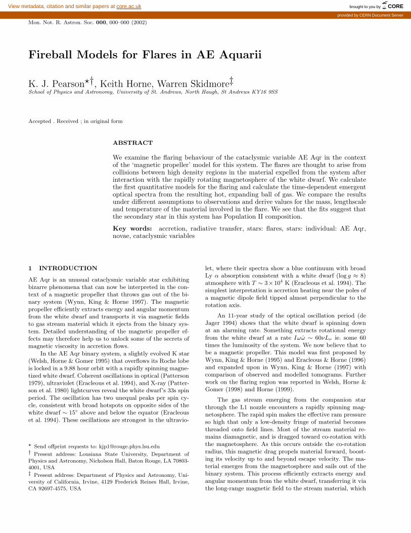
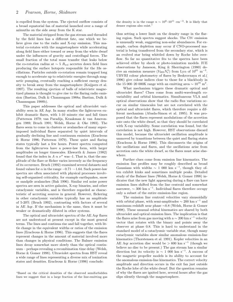
The key insight which solved this puzzle was the realiza-tion that the magnetic propeller acts as a blob sorter. Morecompact, denser, diamagnetic blobs are less affected by mag-netic drag. They punch deeper into the magnetosphere andemerge at a larger azimuth with a smaller terminal velocity.These compact blobs can therefore be overtaken by ‘fluffier’blobs ejected with a larger terminal velocity in the same di-rection, having left the companion star somewhat later butspent less time in the magnetosphere (Wynn, King & Horne1997). The result is a collision between two gas blobs, whichcan give rise to shocks and flares. Calculations of the tra-jectories of magnetically propelled diamagnetic blobs withdifferent drag coefficients indicate that they cross in an arc-shaped region of the exit stream, in just the right placeto account for the orbital kinematics of the emission lines(Welsh, Horne & Gomer 1998; Horne 1999). Figure 1 showshow these trajectories map to a locus of points in the lowerleft quadrant of the Doppler map that is otherwise difficultto populate.

There remains the problem of developing a quantita-tive understanding of the unusual emission-line spectra ofthe blobs. We have two aims for this paper: the principleaim is to see if the observed peak optical flare spectrum canbe reproduced by conditions appropriate to the aftermathof a collision between blobs. The secondary objective is todevelop as far as possible an understanding of the mecha-nisms by which the observed spectra are formed and evolve.We have approached both goals in the spirit of attemptingto find the simplest models that explain the observations.

In section 2 we outline the basic assumptions used inour models. We go on in section 3 to consider the radia-tive transfer problem and calculate analytic expressions forthe behaviour of the optical flare spectra and lightcurvesand outline some numerical considerations . In section 4 wepresent the results of numerical simulations of the flare be-haviour, both lightcurves and spectra, and consider furtherthe limits of applicability of our method. We discuss the in-terpretation of our results in section 5 in terms of the fireballmodel. Finally we summarise our results in section 6.

2 FIREBALL MODELS

2.1 Rough Estimates

We derive rough estimates for the physical parameters asso-ciated with the colliding blobs by using the typical rise timet ∼ 300 s and an observed optical flux fν ∼ 50 mJy with aclosing velocity V ∼ 300 km s−1 for the blobs. We estimatea mass transfer rate

M ∼ 2νLν

V 2=

2νfνd2

V 2≈ 1014 kg s−1 (1)

using a distance of 100pc. This compares to a value fromthe standard evolutionary equation

−M2 ≈ 6× 10−10(

Ph

3

) 53

M�y−1 = 3× 1014 kg s−1 (2)

(Frank, King & Raine 1992). The mean density of the over-flowing gas stream in a CV can be calculated from

ρ =M

QV(3)

Quantity Value

Observed Flux fν 50 mJyClosing Velocity V 300 km s−1

Flare Risetime trise 300 s

Mass Transfer Rate M 1014 kg s−1

Fireball Mass M 3× 1016 kgPre-Collision Lengthscale a 9× 107 m

Initial Temperature T 106 KTotal Energy E 3× 1026 J

Typical Density ρ 3× 10−8 kg m−3

Number Density n 3× 1019 m−3

Column Density N 3× 1027 m−2

Table 1. Estimates of typical values for flare quantities.

where the stream cross-section

Q ≈ 2.4× 1013(

Ts

104 K

)P 2

orb(h) m2 (4)

has been derived by several authors (Papaloizou & Bath1975; Meyer & Meyer-Hofmeister 1983; Hameury, King &Lasota 1986; Ritter 1988; Kovetz, Prialnik & Shara 1988;Sarna 1990; Warner 1995). With a secondary temperatureTs = 4 500 K (Skidmore et al. 2002), we have a mean density,

ρ ≈ 3.2× 10−8(

V

300 km s−1

)−1

kg m−3 (5)

ie.

n ≈ ρ

µmH= 3.2 × 1019 m−3 (6)

where µ ≈ 0.6 is the mean molecular weight appropriate fora fully ionized gas with solar composition. This is consistentwith the lower limits from HST uv observations discussedearlier. It must be remembered that this is the mean densityin a smooth stream. A stream composed of discrete blobs ofmaterial would have range of densities about this value.

We estimate the total mass involved in the collision tobe

M ∼ Mt ∼ 3× 1016 kg. (7)

The typical pre-collision lengthscale a of the problem is givenby

a ∼ V t ∼ 9× 107 m. (8)

Following the collision we might expect a somewhat smallerlengthscale eg.∼ 5×107 m. The above density then suggestsan emission measure Qan2 ≈ 1063 m−3 consistent with theabove IUE measurements for an optically thick Lyα line.

The initial post collision temperature T following astrong shock

T ∼ 3

16

µmHV 2

k≈ 1.2× 106 K. (9)

Finally we have the energy involved in the collision and max-imum possible flare energy E

E ∼ MV 2

8≈ 3× 1026 J. (10)

A summary of typical values is provided in Table 1.


Figure 1. Trajectories of diamagnetic blobs passing though the AE Aquarii system with the corresponding Doppler tomogram.The open circles mark the time of flight in units of 0.1 Porb. Asterisks and grey patches mark the locations where lower densityblobs overtake and collide with more compact blobs, producing fireballs. This occurs in the lower left quadrant at the locationcorresponding to the observed emission lines.

2.2 Initial Conditions

We envision an expanding fireball emerging from the after-math of a collision between two masses m1 + m2 = M . Inthe centre of mass frame, these masses approach with initialvelocities satisfying m1v1 = m2v2. The initial kinetic energyin the centre of mass frame is

E =m1v

21 + m2v

22

2=

MV 2q

2 (1 + q)2(11)

where V = v1 + v2 is the (frame-independent) relative ve-locity and q = m1/m2(= v2/v1) is the mass ratio. Note thatfor a given M and V a range of energies is possible, rangingfrom zero for very extreme mass ratios up to a maximum ofE0 = MV 2/8 for equal masses.

As the collision progresses, some of the energy E is con-verted to thermal energy through dissipation in shocks. Theinitial dissipative phase lasts a short time

ti ∼ ai

V= 300

(ai

108 m

)(V

300 km s−1

)−1

s. (12)

The ratio E/M of energy per mass sets the initial tem-perature Ti and sound speed cs,i through

E

M≈ γkTi

µmH≈ cs,i

2, (13)

where a specific heat ratio γ = 5/3 is appropriate for fullyionized atomic gas. For V ∼ 300 km s−1, Ti ∼ 106 K, so thatthe initial ball of hot gas is atomic and completely ionized.

Since V ∼ cs,i, sound waves have time to cross the initialfireball during the collision time ti, and we therefore expecta roughly uniform temperature profile inside ai.

2.3 Expansion

With nothing to hold it back, the hot ball of gas expandsat the initial sound speed, launching a fireball. We adopt auniform, spherically symmetric, Hubble-like expansion V =

Hr0 = Hr/β, in which the Eulerian radial coordinate r ofa gas element is given in terms of its initial position r0 andtime t by

r(r0, t) = r0 + v(r0)t = r0 + Hr0t = r0(1 + Ht) ≡ r0β. (14)

This defines an expansion factor β which we can use as adimensionless time parameter. The ‘Hubble’ constant is setby the initial conditions Hai ≈ v(ai) ≈ cs,i.

Uniform free expansion is a suitable approximation be-cause the flow becomes supersonic as it expands and cools.If we can determine parameters at some time t = 0 ie. β = 1for the lengthscale (a0), temperature (T0) and mass (M) wecan derive the time evolution as follows. We adopt a Gaus-sian density profile

ρ(r, t) = ρ0β−3e−η2

(15)

where

ρ0 =M

(πa20)

32

(16)

is the initial central density and

η ≡ r0

a0=

r

a(17)

is a dimensionless radius coordinate, the radius r scaled tothe lengthscale a = βa0.

Although this Gaussian density profile is only a guess,it is motivated by the Gaussian shapes of observed velocityprofiles, and by the thought that the initial thermal velocitydistribution in the hot gas will map into the density profileof the expanding fireball because the fast particles travelfarther than slow ones.

2.4 Cooling

We consider three cooling schemes: adiabatic, isothermaland radiative. The adiabatic fireball cools purely as a re-sult of its expansion and corresponds to a situation where


the radiative and recombination cooling rates are negligible.In contrast, the isothermal model maintains a fixed temper-ature throughout its evolution. A truly isothermal fireballwould require a finely balanced energy source to counter-act the expansion cooling. However, it may an appropriateapproximation to a situation where a photospheric regiondominates the emission and presents a fixed effective tem-perature to the observer as a result of the stong dependenceof opacity on temperature. The radiative models cool adia-batically throughout and as a result of radiation from a thinzone near the photosphere which we model by immediatelydropping the temperature to Tp ∼ 104 K at this surface.

2.4.1 Adiabatic Cooling

During adiabatic expansion, P ∝ ργ and T ∝ P/ρ ∝ ργ−1.If we consider the evolution of a given gas element then,with ρ ∝ β−3, the temperature decreases with time as

T (r, t) = T0(r0)β−3(γ−1). (18)

We see that an initially uniform temperature distributionremains uniform and so, for this case, we can write, moresimply,

T (r, t) = T0β−3(γ−1). (19)

With γ = 5/3 for a monatomic gas, T ∝ β−2, and so thesound speed cs ∝ T 1/2 ∝ β−1. The sound crossing timea/cs ∝ β2. The fireball becomes almost immediately super-sonic. We can derive the behaviour of the sonic point fromthe definition that it is the position where the expansionrate matches the sound speed. Thus,

1 ≡ v(rs, t)

cs(t)=

Hrs,0

cs(t)=

Hrs

βcs(t)=

Hrs

cs,0. (20)

Assuming a uniform temperature profile and γ = 5/3, thisgives

rs =cs,0

H= a0. (21)

Hence, we can see that the sonic point remains fixed in spaceat a0. The initial density structure emerging through thesonic surface at radius a0 is subsequently ‘frozen in’ by therapid expansion.

2.4.2 Radiative Cooling Timescales

The time required for the fireball to radiate away its in-ternal energy depends crucially on the temperature of thephotosphere (assuming that the fireball is optically thick).For a uniform temperature distribution the timescale is veryshort:

U

U∼ Mk

mHσR2T 3(22)

= 1.5

(M

1017 kg

)(R

108 m

)−2 ( T

104 K

)−3

s. (23)

We would thus expect the region from which the radiationescapes to cool rapidly until the region becomes opticallythin and the cooling efficiency drops.

If the photospheric temperature Tp is significantly

cooler than the optically thick region, the radiative timescale

U

U∼ MkT

mHσR2T 4p

(24)

= 150

(M

1017 kg

)(R

108 m

)−2

×(

T

106 K

)(Tp

104 K

)−4

s (25)

can become comparable to the evolutionary timescale of thefireball.

2.4.3 Radiative Cooling Front

Following the exact behaviour of radiative cooling and heat-ing is a complex process requiring us to follow the behaviourof the internal radiation field of the fireball through theoptically thick to optically thin transition. Such detailedmodelling is beyond the scope of the initial investigationspresented here. We note that studies of cooling from op-tically thin plasmas (Lynden-Bell & Tout 2001; Dalgarno& McCray 1972) show that there is a significant reductionin efficiency due to hydrogen recombination and the con-sequent loss of free electrons below approximately 104 K.Since the photosphere is the region where the optical depthfor escaping radiation is unity, this suggests that the photo-sphere may adopt a roughly constant effective temperatureTp ∼ 104 K. The relatively dense material in the fireballwill be able to cool rapidly down to this temperature beforethe cooling rate stalls. We approximate a radiatively coolingfireball by maintaining a hot core region which cools adia-batically as it expands. Once gas elements cross the bound-ary to this region, we assume them to cool immediately tothe effective temperature of the photosphere and thereafteradiabatically. We derive the radius of the photospheric sur-face below, using the blackbody luminosity and the thermalenergy of the central region.

To find the photospheric radius rp = a0βηp in our ra-diative model we calculate the total thermal energy in asphere of radius rp

U =

∫ rp

0

3

2

ρkT

µmH4πr2dr (26)

=6πk

µmH

T0a30ρc,0

β3(γ−1)

∫ ηp

0

e−η2η2dη. (27)

Hence, differentiating,

∂U

∂ηp=

6πkT0a30ρc,0

µmHβ3(γ−1)η2pe−η2

p . (28)

Radiative cooling at fixed effective temperature Tp gives

∂U

∂β= −4πHa2

0β2η2

pσT 4p (29)

and so, using

∂ηp

∂β≡(

∂U

∂β

)(∂U

∂ηp

)−1

, (30)

we have the differential equation for the core radius as afunction of time

∂ηp

∂βe−η2

p = −Cβ3γ−1, (31)


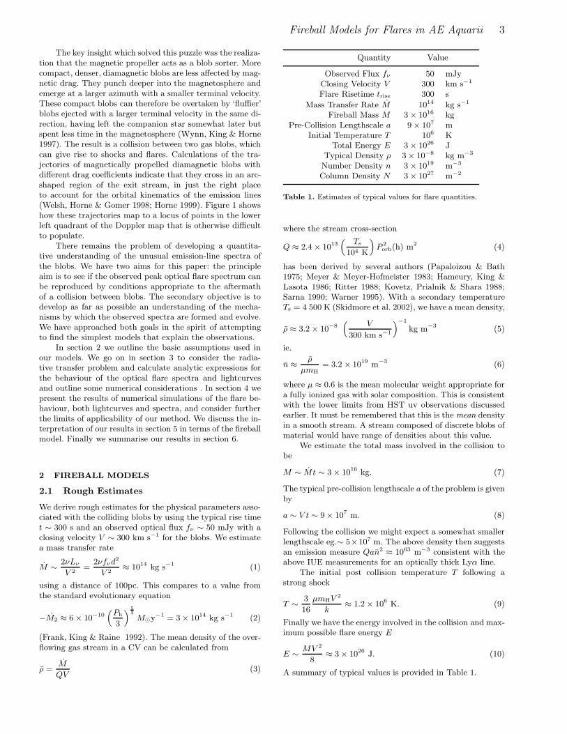
Figure 2. The evolution of the temperature boundary for theradiative model with M = 6.8 × 1016 kg, a0 = 9.6 × 107 m andT0 = 18 000 K. The solid line is for Tp = 10 000 K and thedashed line for Tp = 18 000 K. In each case we have initial valuesfor ηp = 2, 3, 4, 5.

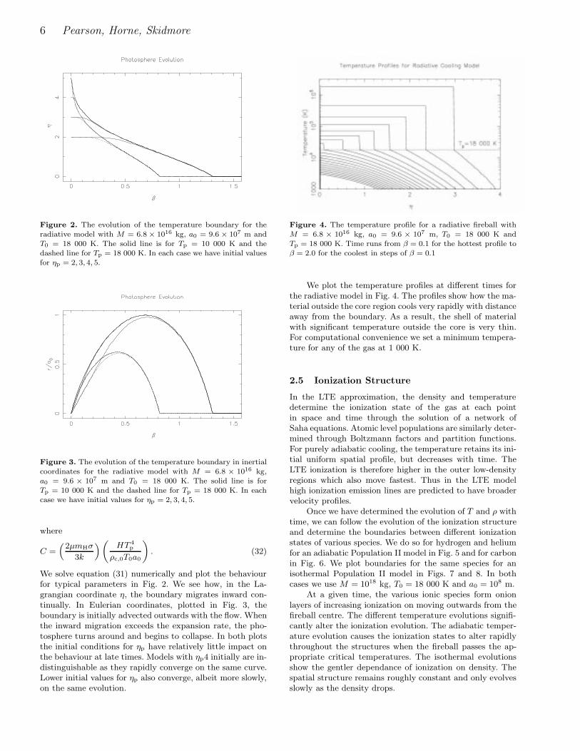
Figure 3. The evolution of the temperature boundary in inertialcoordinates for the radiative model with M = 6.8 × 1016 kg,a0 = 9.6 × 107 m and T0 = 18 000 K. The solid line is forTp = 10 000 K and the dashed line for Tp = 18 000 K. In eachcase we have initial values for ηp = 2, 3, 4, 5.

where

C =(

2µmHσ

3k

)( HT 4p

ρc,0T0a0

). (32)

We solve equation (31) numerically and plot the behaviourfor typical parameters in Fig. 2. We see how, in the La-grangian coordinate η, the boundary migrates inward con-tinually. In Eulerian coordinates, plotted in Fig. 3, theboundary is initially advected outwards with the flow. Whenthe inward migration exceeds the expansion rate, the pho-tosphere turns around and begins to collapse. In both plotsthe initial conditions for ηp have relatively little impact onthe behaviour at late times. Models with ηp4 initially are in-distinguishable as they rapidly converge on the same curve.Lower initial values for ηp also converge, albeit more slowly,on the same evolution.

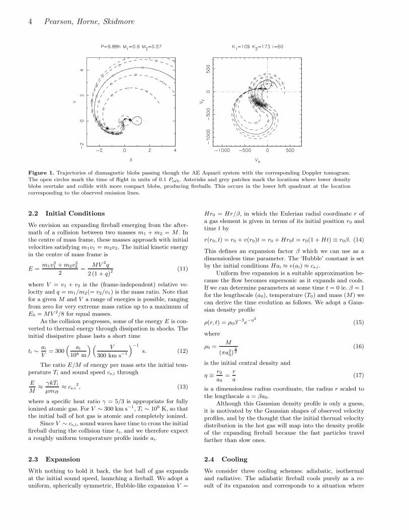
Figure 4. The temperature profile for a radiative fireball withM = 6.8 × 1016 kg, a0 = 9.6 × 107 m, T0 = 18 000 K andTp = 18 000 K. Time runs from β = 0.1 for the hottest profile toβ = 2.0 for the coolest in steps of β = 0.1

We plot the temperature profiles at different times forthe radiative model in Fig. 4. The profiles show how the ma-terial outside the core region cools very rapidly with distanceaway from the boundary. As a result, the shell of materialwith significant temperature outside the core is very thin.For computational convenience we set a minimum tempera-ture for any of the gas at 1 000 K.

2.5 Ionization Structure

In the LTE approximation, the density and temperaturedetermine the ionization state of the gas at each pointin space and time through the solution of a network ofSaha equations. Atomic level populations are similarly deter-mined through Boltzmann factors and partition functions.For purely adiabatic cooling, the temperature retains its ini-tial uniform spatial profile, but decreases with time. TheLTE ionization is therefore higher in the outer low-densityregions which also move fastest. Thus in the LTE modelhigh ionization emission lines are predicted to have broadervelocity profiles.

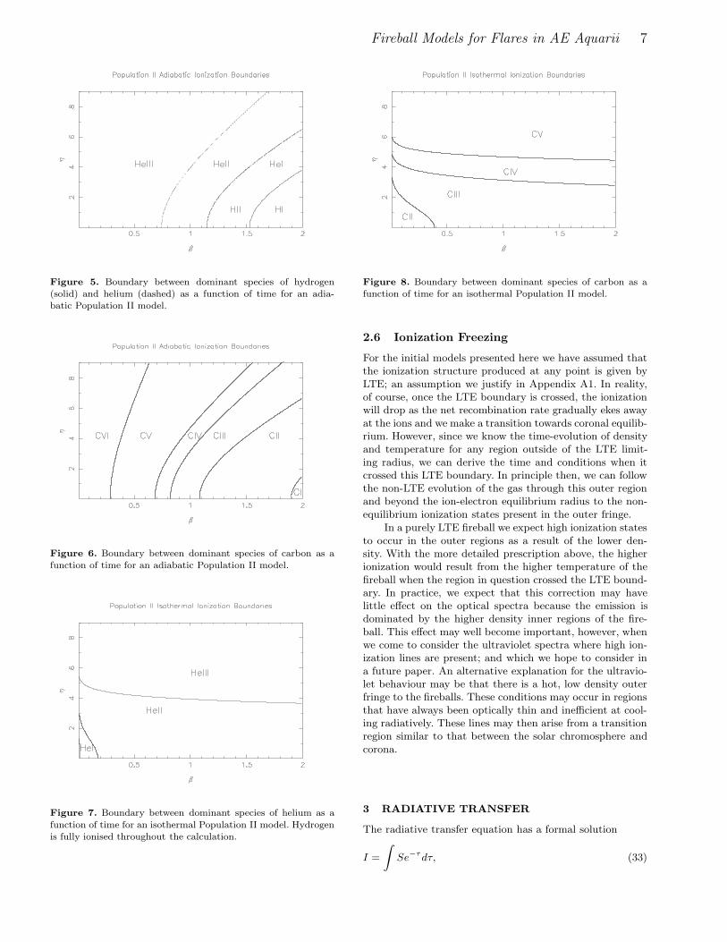
Once we have determined the evolution of T and ρ withtime, we can follow the evolution of the ionization structureand determine the boundaries between different ionizationstates of various species. We do so for hydrogen and heliumfor an adiabatic Population II model in Fig. 5 and for carbonin Fig. 6. We plot boundaries for the same species for anisothermal Population II model in Figs. 7 and 8. In bothcases we use M = 1018 kg, T0 = 18 000 K and a0 = 108 m.

At a given time, the various ionic species form onionlayers of increasing ionization on moving outwards from thefireball centre. The different temperature evolutions signifi-cantly alter the ionization evolution. The adiabatic temper-ature evolution causes the ionization states to alter rapidlythroughout the structures when the fireball passes the ap-propriate critical temperatures. The isothermal evolutionsshow the gentler dependance of ionization on density. Thespatial structure remains roughly constant and only evolvesslowly as the density drops.


Figure 5. Boundary between dominant species of hydrogen(solid) and helium (dashed) as a function of time for an adia-batic Population II model.

Figure 6. Boundary between dominant species of carbon as afunction of time for an adiabatic Population II model.

Figure 7. Boundary between dominant species of helium as a

function of time for an isothermal Population II model. Hydrogenis fully ionised throughout the calculation.

Figure 8. Boundary between dominant species of carbon as afunction of time for an isothermal Population II model.

2.6 Ionization Freezing

For the initial models presented here we have assumed thatthe ionization structure produced at any point is given byLTE; an assumption we justify in Appendix A1. In reality,of course, once the LTE boundary is crossed, the ionizationwill drop as the net recombination rate gradually ekes awayat the ions and we make a transition towards coronal equilib-rium. However, since we know the time-evolution of densityand temperature for any region outside of the LTE limit-ing radius, we can derive the time and conditions when itcrossed this LTE boundary. In principle then, we can followthe non-LTE evolution of the gas through this outer regionand beyond the ion-electron equilibrium radius to the non-equilibrium ionization states present in the outer fringe.

In a purely LTE fireball we expect high ionization statesto occur in the outer regions as a result of the lower den-sity. With the more detailed prescription above, the higherionization would result from the higher temperature of thefireball when the region in question crossed the LTE bound-ary. In practice, we expect that this correction may havelittle effect on the optical spectra because the emission isdominated by the higher density inner regions of the fire-ball. This effect may well become important, however, whenwe come to consider the ultraviolet spectra where high ion-ization lines are present; and which we hope to consider ina future paper. An alternative explanation for the ultravio-let behaviour may be that there is a hot, low density outerfringe to the fireballs. These conditions may occur in regionsthat have always been optically thin and inefficient at cool-ing radiatively. These lines may then arise from a transitionregion similar to that between the solar chromosphere andcorona.

3 RADIATIVE TRANSFER

The radiative transfer equation has a formal solution

I =

∫Se−τdτ, (33)


where I is the intensity of the emerging radiation, S is thesource function, and τ is the optical depth measured alongthe line of sight from the observer. This integral sums contri-butions Sdτ to the radiation intensity, attenuating each bythe factor e−τ because it has to pass through optical depthτ to reach the observer.

Since we have assumed LTE, the source function is thePlanck function, and opacities both for lines and continuumare also known once the velocity, temperature, and densityprofiles and element abundances are specified. The integralcan therefore be evaluated numerically, either in this formor more quickly by using Sobolev resonant surface approxi-mations.

The above line integral gives the intensity I(y) for linesof sight with different impact parameters y. We let x mea-sure distance from the fireball centre toward the observer,and y the distance perpendicular to the line of sight. Thefireball flux, obtained by summing intensities weighted bythe solid angles of annuli on the sky, is then

f(λ) =

∫ ∞

0

I(λ, y)2πy

d2dy (34)

where d is the source distance.

3.1 Continuum Lightcurves and Spectra

In a forthcoming paper (Pearson, Horne & Skidmore, inprep.) we will consider generic analytic models for fireballbehaviour applicable to a variety of systems. We use thegeneral opacity given in equation (A4). We quote here anapproximation to the lightcurve behaviour being the sum ofoptically thick and optically thin contributions:

fν = fν,0β20τ b

0s (τ0) (35)

where

fν,0 =πa2

0

2d2Bν(T ), (36)

β0 =

[ε

ν3

κ1M2

√2πT0π3a5

0

] 210−Γ

, (37)

ε = 1− e−hνkT (38)

τ0 =

(β0

β

) 10−Γ2

, (39)

b =6− Γ

10− Γ, (40)

s(τ ) =

{1 τ < 11 + ln τ

ττ ≥ 1

. (41)

Here β0 is the time that the fireball first becomes opticallythin through its centre and τ0 is the current optical depththrough the fireball centre.

The peak flux occurs when

τ0 = eb

1−b (42)

which occurs at a time

βpk = β0e− b

2 . (43)

We note that equations (37) and (43) predict that the peakflux will occur at different times for different wavelengths.

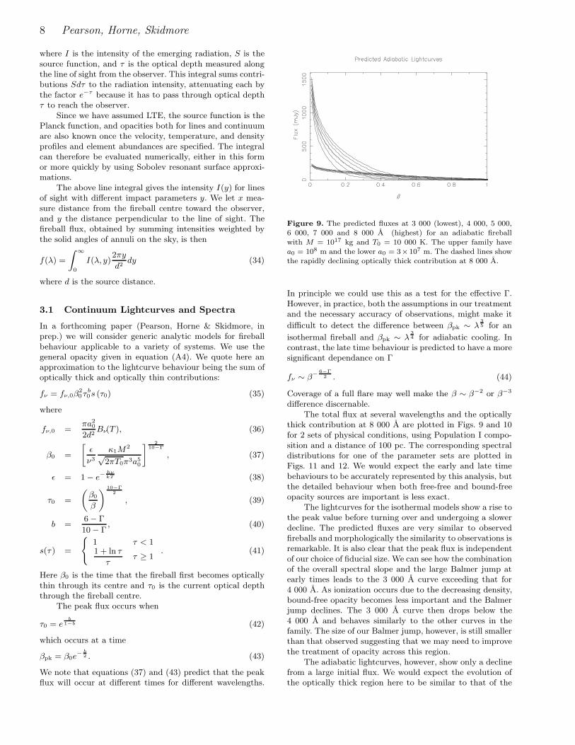
Figure 9. The predicted fluxes at 3 000 (lowest), 4 000, 5 000,6 000, 7 000 and 8 000 A (highest) for an adiabatic fireballwith M = 1017 kg and T0 = 10 000 K. The upper family havea0 = 108 m and the lower a0 = 3×107 m. The dashed lines showthe rapidly declining optically thick contribution at 8 000 A.

In principle we could use this as a test for the effective Γ.However, in practice, both the assumptions in our treatmentand the necessary accuracy of observations, might make it

difficult to detect the difference between βpk ∼ λ35 for an

isothermal fireball and βpk ∼ λ34 for adiabatic cooling. In

contrast, the late time behaviour is predicted to have a moresignificant dependance on Γ

fν ∼ β−6−Γ

2 . (44)

Coverage of a full flare may well make the β ∼ β−2 or β−3

difference discernable.The total flux at several wavelengths and the optically

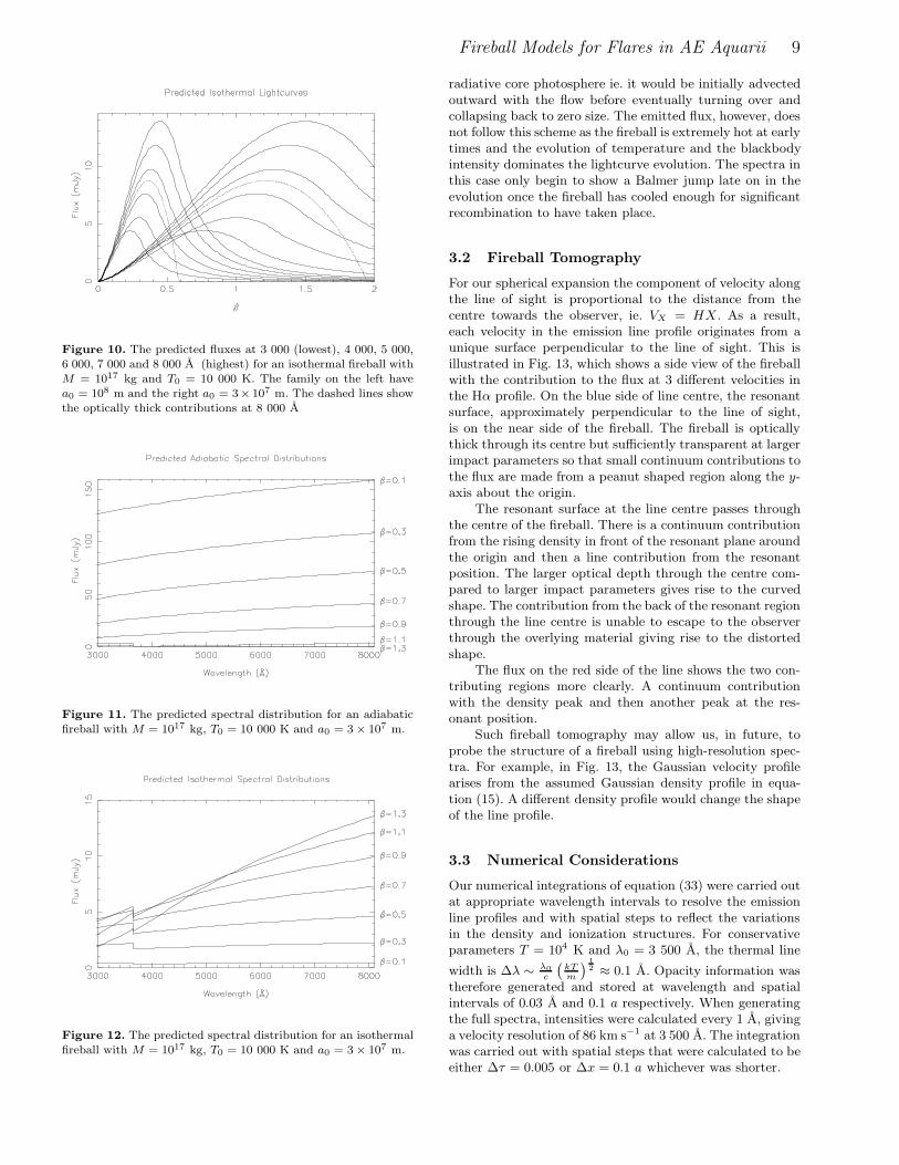
thick contribution at 8 000 A are plotted in Figs. 9 and 10for 2 sets of physical conditions, using Population I compo-sition and a distance of 100 pc. The corresponding spectraldistributions for one of the parameter sets are plotted inFigs. 11 and 12. We would expect the early and late timebehaviours to be accurately represented by this analysis, butthe detailed behaviour when both free-free and bound-freeopacity sources are important is less exact.

The lightcurves for the isothermal models show a rise tothe peak value before turning over and undergoing a slowerdecline. The predicted fluxes are very similar to observedfireballs and morphologically the similarity to observations isremarkable. It is also clear that the peak flux is independentof our choice of fiducial size. We can see how the combinationof the overall spectral slope and the large Balmer jump atearly times leads to the 3 000 A curve exceeding that for4 000 A. As ionization occurs due to the decreasing density,bound-free opacity becomes less important and the Balmerjump declines. The 3 000 A curve then drops below the4 000 A and behaves similarly to the other curves in thefamily. The size of our Balmer jump, however, is still smallerthan that observed suggesting that we may need to improvethe treatment of opacity across this region.

The adiabatic lightcurves, however, show only a declinefrom a large initial flux. We would expect the evolution ofthe optically thick region here to be similar to that of the


Figure 10. The predicted fluxes at 3 000 (lowest), 4 000, 5 000,6 000, 7 000 and 8 000 A (highest) for an isothermal fireball withM = 1017 kg and T0 = 10 000 K. The family on the left havea0 = 108 m and the right a0 = 3× 107 m. The dashed lines showthe optically thick contributions at 8 000 A

Figure 11. The predicted spectral distribution for an adiabaticfireball with M = 1017 kg, T0 = 10 000 K and a0 = 3× 107 m.

Figure 12. The predicted spectral distribution for an isothermalfireball with M = 1017 kg, T0 = 10 000 K and a0 = 3× 107 m.

radiative core photosphere ie. it would be initially advectedoutward with the flow before eventually turning over andcollapsing back to zero size. The emitted flux, however, doesnot follow this scheme as the fireball is extremely hot at earlytimes and the evolution of temperature and the blackbodyintensity dominates the lightcurve evolution. The spectra inthis case only begin to show a Balmer jump late on in theevolution once the fireball has cooled enough for significantrecombination to have taken place.

3.2 Fireball Tomography

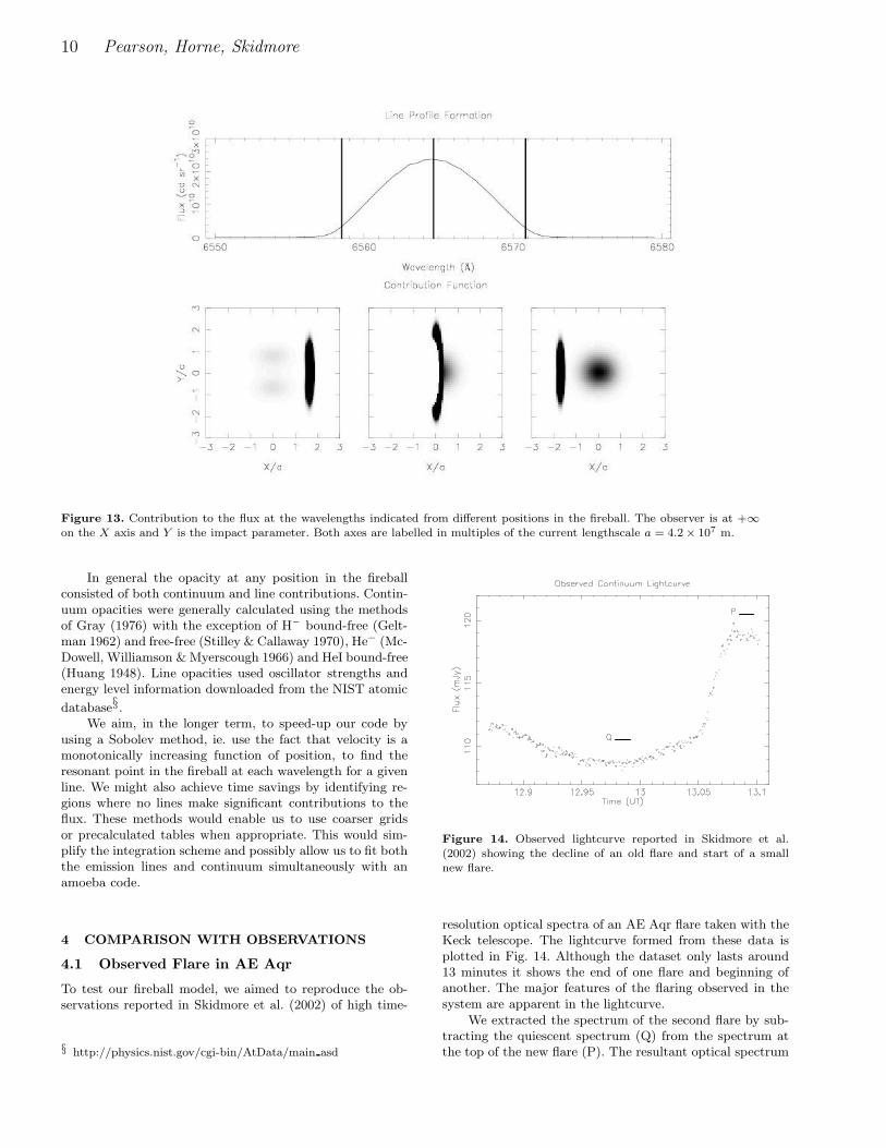
For our spherical expansion the component of velocity alongthe line of sight is proportional to the distance from thecentre towards the observer, ie. VX = HX. As a result,each velocity in the emission line profile originates from aunique surface perpendicular to the line of sight. This isillustrated in Fig. 13, which shows a side view of the fireballwith the contribution to the flux at 3 different velocities inthe Hα profile. On the blue side of line centre, the resonantsurface, approximately perpendicular to the line of sight,is on the near side of the fireball. The fireball is opticallythick through its centre but sufficiently transparent at largerimpact parameters so that small continuum contributions tothe flux are made from a peanut shaped region along the y-axis about the origin.

The resonant surface at the line centre passes throughthe centre of the fireball. There is a continuum contributionfrom the rising density in front of the resonant plane aroundthe origin and then a line contribution from the resonantposition. The larger optical depth through the centre com-pared to larger impact parameters gives rise to the curvedshape. The contribution from the back of the resonant regionthrough the line centre is unable to escape to the observerthrough the overlying material giving rise to the distortedshape.

The flux on the red side of the line shows the two con-tributing regions more clearly. A continuum contributionwith the density peak and then another peak at the res-onant position.

Such fireball tomography may allow us, in future, toprobe the structure of a fireball using high-resolution spec-tra. For example, in Fig. 13, the Gaussian velocity profilearises from the assumed Gaussian density profile in equa-tion (15). A different density profile would change the shapeof the line profile.

3.3 Numerical Considerations

Our numerical integrations of equation (33) were carried outat appropriate wavelength intervals to resolve the emissionline profiles and with spatial steps to reflect the variationsin the density and ionization structures. For conservativeparameters T = 104 K and λ0 = 3 500 A, the thermal line

width is ∆λ ∼ λ0c

(kTm

) 12 ≈ 0.1 A. Opacity information was

therefore generated and stored at wavelength and spatialintervals of 0.03 A and 0.1 a respectively. When generatingthe full spectra, intensities were calculated every 1 A, givinga velocity resolution of 86 km s−1 at 3 500 A. The integrationwas carried out with spatial steps that were calculated to beeither ∆τ = 0.005 or ∆x = 0.1 a whichever was shorter.


Figure 13. Contribution to the flux at the wavelengths indicated from different positions in the fireball. The observer is at +∞on the X axis and Y is the impact parameter. Both axes are labelled in multiples of the current lengthscale a = 4.2× 107 m.

In general the opacity at any position in the fireballconsisted of both continuum and line contributions. Contin-uum opacities were generally calculated using the methodsof Gray (1976) with the exception of H− bound-free (Gelt-man 1962) and free-free (Stilley & Callaway 1970), He− (Mc-Dowell, Williamson & Myerscough 1966) and HeI bound-free(Huang 1948). Line opacities used oscillator strengths andenergy level information downloaded from the NIST atomic

database§.We aim, in the longer term, to speed-up our code by

using a Sobolev method, ie. use the fact that velocity is amonotonically increasing function of position, to find theresonant point in the fireball at each wavelength for a givenline. We might also achieve time savings by identifying re-gions where no lines make significant contributions to theflux. These methods would enable us to use coarser gridsor precalculated tables when appropriate. This would sim-plify the integration scheme and possibly allow us to fit boththe emission lines and continuum simultaneously with anamoeba code.

4 COMPARISON WITH OBSERVATIONS

4.1 Observed Flare in AE Aqr

To test our fireball model, we aimed to reproduce the ob-servations reported in Skidmore et al. (2002) of high time-

§ http://physics.nist.gov/cgi-bin/AtData/main asd

Figure 14. Observed lightcurve reported in Skidmore et al.(2002) showing the decline of an old flare and start of a smallnew flare.

resolution optical spectra of an AE Aqr flare taken with theKeck telescope. The lightcurve formed from these data isplotted in Fig. 14. Although the dataset only lasts around13 minutes it shows the end of one flare and beginning ofanother. The major features of the flaring observed in thesystem are apparent in the lightcurve.

We extracted the spectrum of the second flare by sub-tracting the quiescent spectrum (Q) from the spectrum atthe top of the new flare (P). The resultant optical spectrum


Line Fitted FWHM Deconvolved FWHM(km s−1) (km s−1)

Hα 1909 ± 7 1856 ± 7HeI 5876 1510 ± 6 1424 ± 6HeI 4922 1353 ± 13 1214 ± 13

Hβ 1681 ± 3 1569 ± 3Hγ 1743 ± 3 1589 ± 3Hδ 2171 ± 4 2050 ± 4Hε 1645 ± 5 1469 ± 5

CaH 2423 ± 21 2306 ± 21

Table 2. Fitted and deconvolved widths of several emission lines.

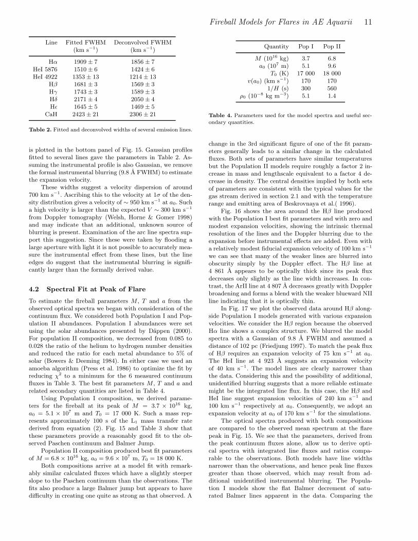
is plotted in the bottom panel of Fig. 15. Gaussian profilesfitted to several lines gave the parameters in Table 2. As-suming the instrumental profile is also Gaussian, we removethe formal instrumental blurring (9.8 A FWHM) to estimatethe expansion velocity.

These widths suggest a velocity dispersion of around700 km s−1. Ascribing this to the velocity at 1σ of the den-sity distribution gives a velocity of ∼ 950 km s−1 at a0. Sucha high velocity is larger than the expected V ∼ 300 km s−1

from Doppler tomography (Welsh, Horne & Gomer 1998)and may indicate that an additional, unknown source ofblurring is present. Examination of the arc line spectra sup-port this suggestion. Since these were taken by flooding alarge aperture with light it is not possible to accurately mea-sure the instrumental effect from these lines, but the lineedges do suggest that the instrumental blurring is signifi-cantly larger than the formally derived value.

4.2 Spectral Fit at Peak of Flare

To estimate the fireball parameters M , T and a from theobserved optical spectra we began with consideration of thecontinuum flux. We considered both Population I and Pop-ulation II abundances. Population I abundances were setusing the solar abundances presented by Dappen (2000).For population II composition, we decreased from 0.085 to0.028 the ratio of the helium to hydrogen number densitiesand reduced the ratio for each metal abundance to 5% ofsolar (Bowers & Deeming 1984). In either case we used anamoeba algorithm (Press et al. 1986) to optimize the fit byreducing χ2 to a minimum for the 6 measured continuumfluxes in Table 3. The best fit parameters M , T and a andrelated secondary quantities are listed in Table 4.

Using Population I composition, we derived parame-ters for the fireball at its peak of M = 3.7 × 1016 kg,a0 = 5.1 × 107 m and T0 = 17 000 K. Such a mass rep-resents approximately 100 s of the L1 mass transfer ratederived from equation (2). Fig. 15 and Table 3 show thatthese parameters provide a reasonably good fit to the ob-served Paschen continuum and Balmer Jump.

Population II composition produced best fit parametersof M = 6.8× 1016 kg, a0 = 9.6× 107 m, T0 = 18 000 K.

Both compositions arrive at a model fit with remark-ably similar calculated fluxes which have a slightly steeperslope to the Paschen continuum than the observations. Thefits also produce a large Balmer jump but appears to havedifficulty in creating one quite as strong as that observed. A

Quantity Pop I Pop II

M (1016 kg) 3.7 6.8a0 (107 m) 5.1 9.6

T0 (K) 17 000 18 000v(a0) (km s−1) 170 170

1/H (s) 300 560ρ0 (10−8 kg m−3) 5.1 1.4

Table 4. Parameters used for the model spectra and useful sec-ondary quantities.

change in the 3rd significant figure of one of the fit param-eters generally leads to a similar change in the calculatedfluxes. Both sets of parameters have similar temperaturesbut the Population II models require roughly a factor 2 in-crease in mass and lengthscale equivalent to a factor 4 de-crease in density. The central densities implied by both setsof parameters are consistent with the typical values for thegas stream derived in section 2.1 and with the temperaturerange and emitting area of Beskrovnaya et al.( 1996).

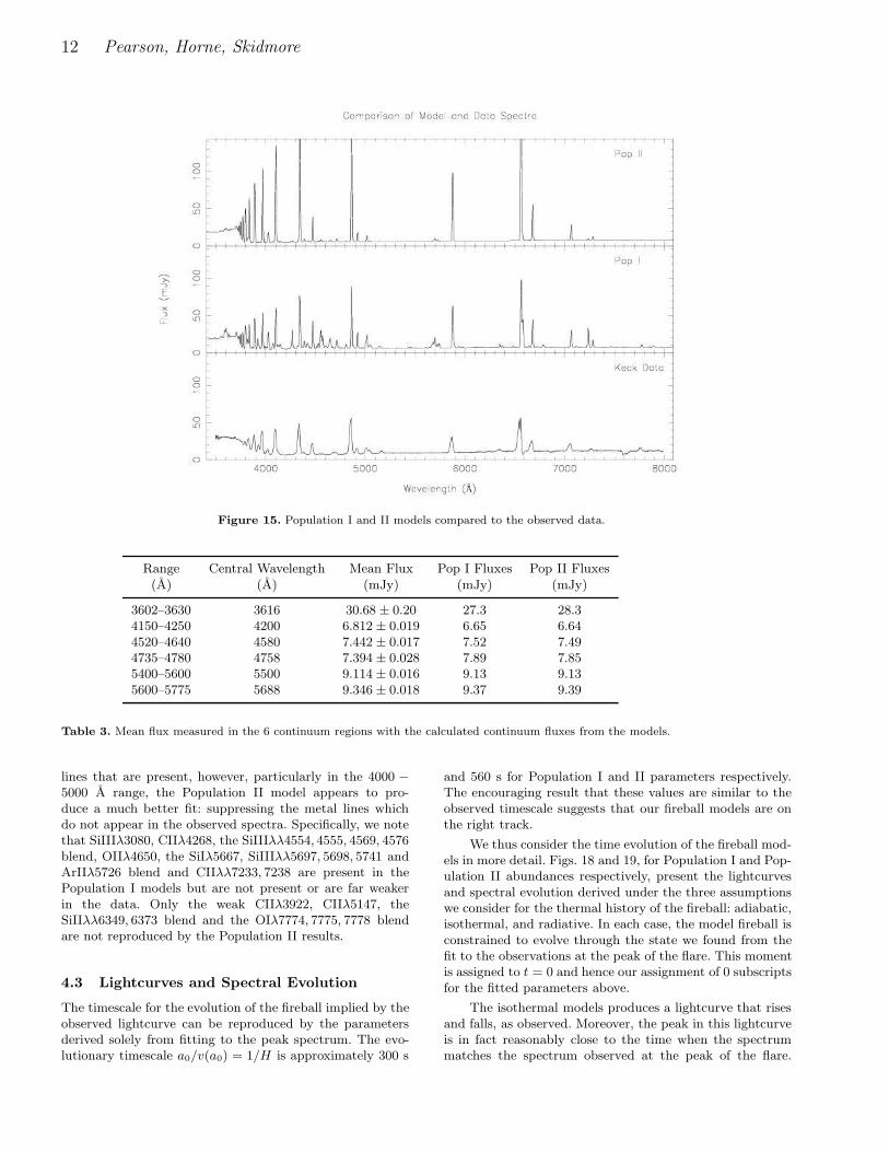
Fig. 16 shows the area around the Hβ line producedwith the Population I best fit parameters and with zero andmodest expansion velocities, showing the intrinsic thermalresolution of the lines and the Doppler blurring due to theexpansion before instrumental effects are added. Even witha relatively modest fiducial expansion velocity of 100 km s−1

we can see that many of the weaker lines are blurred intoobscurity simply by the Doppler effect. The Hβ line at4 861 A appears to be optically thick since its peak fluxdecreases only slightly as the line width increases. In con-trast, the ArII line at 4 807 A decreases greatly with Dopplerbroadening and forms a blend with the weaker blueward NIIline indicating that it is optically thin.

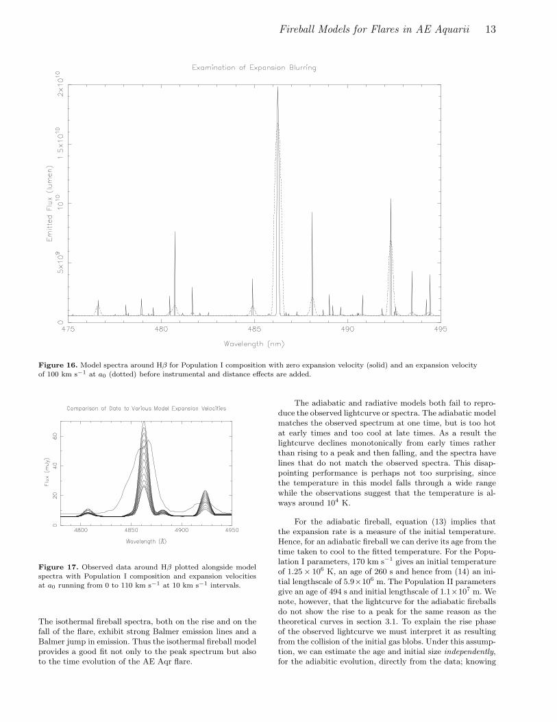
In Fig. 17 we plot the observed data around Hβ along-side Population I models generated with various expansionvelocities. We consider the Hβ region because the observedHα line shows a complex structure. We blurred the modelspectra with a Gaussian of 9.8 A FWHM and assumed adistance of 102 pc (Friedjung 1997). To match the peak fluxof Hβ requires an expansion velocity of 75 km s−1 at a0.The HeI line at 4 923 A suggests an expansion velocityof 40 km s−1. The model lines are clearly narrower thanthe data. Considering this and the possibility of additional,unidentified blurring suggests that a more reliable estimatemight be the integrated line flux. In this case, the Hβ andHeI line suggest expansion velocities of 240 km s−1 and100 km s−1 respectively at a0. Consequently, we adopt anexpansion velocity at a0 of 170 km s−1 for the simulations.

The optical spectra produced with both compositionsare compared to the observed mean spectrum at the flarepeak in Fig. 15. We see that the parameters, derived fromthe peak continuum fluxes alone, allow us to derive opti-cal spectra with integrated line fluxes and ratios compa-rable to the observations. Both models have line widthsnarrower than the observations, and hence peak line fluxesgreater than those observed, which may result from ad-ditional unidentified instrumental blurring. The Popula-tion I models show the flat Balmer decrement of satu-rated Balmer lines apparent in the data. Comparing the


Figure 15. Population I and II models compared to the observed data.

Range Central Wavelength Mean Flux Pop I Fluxes Pop II Fluxes(A) (A) (mJy) (mJy) (mJy)

3602–3630 3616 30.68 ± 0.20 27.3 28.34150–4250 4200 6.812 ± 0.019 6.65 6.644520–4640 4580 7.442 ± 0.017 7.52 7.494735–4780 4758 7.394 ± 0.028 7.89 7.855400–5600 5500 9.114 ± 0.016 9.13 9.135600–5775 5688 9.346 ± 0.018 9.37 9.39

Table 3. Mean flux measured in the 6 continuum regions with the calculated continuum fluxes from the models.

lines that are present, however, particularly in the 4000 −5000 A range, the Population II model appears to pro-duce a much better fit: suppressing the metal lines whichdo not appear in the observed spectra. Specifically, we notethat SiIIIλ3080, CIIλ4268, the SiIIIλλ4554, 4555, 4569, 4576blend, OIIλ4650, the SiIλ5667, SiIIIλλ5697, 5698, 5741 andArIIλ5726 blend and CIIλλ7233, 7238 are present in thePopulation I models but are not present or are far weakerin the data. Only the weak CIIλ3922, CIIλ5147, theSiIIλλ6349, 6373 blend and the OIλ7774, 7775, 7778 blendare not reproduced by the Population II results.

4.3 Lightcurves and Spectral Evolution

The timescale for the evolution of the fireball implied by theobserved lightcurve can be reproduced by the parametersderived solely from fitting to the peak spectrum. The evo-lutionary timescale a0/v(a0) = 1/H is approximately 300 s

and 560 s for Population I and II parameters respectively.The encouraging result that these values are similar to theobserved timescale suggests that our fireball models are onthe right track.

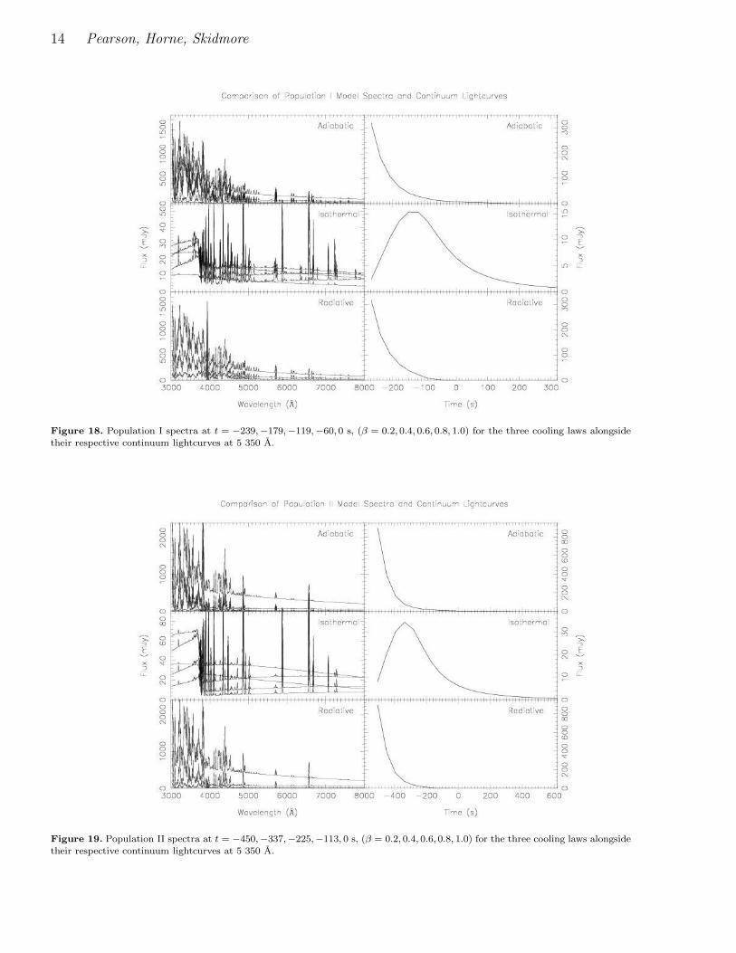
We thus consider the time evolution of the fireball mod-els in more detail. Figs. 18 and 19, for Population I and Pop-ulation II abundances respectively, present the lightcurvesand spectral evolution derived under the three assumptionswe consider for the thermal history of the fireball: adiabatic,isothermal, and radiative. In each case, the model fireball isconstrained to evolve through the state we found from thefit to the observations at the peak of the flare. This momentis assigned to t = 0 and hence our assignment of 0 subscriptsfor the fitted parameters above.

The isothermal models produces a lightcurve that risesand falls, as observed. Moreover, the peak in this lightcurveis in fact reasonably close to the time when the spectrummatches the spectrum observed at the peak of the flare.


Figure 16. Model spectra around Hβ for Population I composition with zero expansion velocity (solid) and an expansion velocityof 100 km s−1 at a0 (dotted) before instrumental and distance effects are added.

Figure 17. Observed data around Hβ plotted alongside modelspectra with Population I composition and expansion velocitiesat a0 running from 0 to 110 km s−1 at 10 km s−1 intervals.

The isothermal fireball spectra, both on the rise and on thefall of the flare, exhibit strong Balmer emission lines and aBalmer jump in emission. Thus the isothermal fireball modelprovides a good fit not only to the peak spectrum but alsoto the time evolution of the AE Aqr flare.

The adiabatic and radiative models both fail to repro-duce the observed lightcurve or spectra. The adiabatic modelmatches the observed spectrum at one time, but is too hotat early times and too cool at late times. As a result thelightcurve declines monotonically from early times ratherthan rising to a peak and then falling, and the spectra havelines that do not match the observed spectra. This disap-pointing performance is perhaps not too surprising, sincethe temperature in this model falls through a wide rangewhile the observations suggest that the temperature is al-ways around 104 K.

For the adiabatic fireball, equation (13) implies thatthe expansion rate is a measure of the initial temperature.Hence, for an adiabatic fireball we can derive its age from thetime taken to cool to the fitted temperature. For the Popu-lation I parameters, 170 km s−1 gives an initial temperatureof 1.25× 106 K, an age of 260 s and hence from (14) an ini-tial lengthscale of 5.9×106 m. The Population II parametersgive an age of 494 s and initial lengthscale of 1.1×107 m. Wenote, however, that the lightcurve for the adiabatic fireballsdo not show the rise to a peak for the same reason as thetheoretical curves in section 3.1. To explain the rise phaseof the observed lightcurve we must interpret it as resultingfrom the collision of the initial gas blobs. Under this assump-tion, we can estimate the age and initial size independently,for the adiabitic evolution, directly from the data; knowing


Figure 18. Population I spectra at t = −239,−179,−119,−60, 0 s, (β = 0.2, 0.4, 0.6, 0.8, 1.0) for the three cooling laws alongsidetheir respective continuum lightcurves at 5 350 A.

Figure 19. Population II spectra at t = −450,−337,−225,−113, 0 s, (β = 0.2, 0.4, 0.6, 0.8, 1.0) for the three cooling laws alongsidetheir respective continuum lightcurves at 5 350 A.


the rise time of the flare and the typical closing velocities:

tage ∼ trise = 63 s (45)

l ∼ V trise = 3× 105 × 60 = 1.8× 107 m. (46)

The radiative model looks roughly the same as the adia-batic model. This occurs because the cooling front (as shownin Fig. 4) occurs well outside the photosphere. We therefore“see” into the adiabatically-cooling core. This is not con-sistent with our assumption that the rapid cooling occursnear the photosphere as a result of the opacity drop thereand suggests that a more sophisticated approach involvingheating of the gas by emergent photons may be required foran accurate treatment of such a model.

5 DISCUSSION

The spectra produced with Population II composition re-produce the optical observations well. The fitted parametersare consistent with both the expected conditions in the masstransfer stream and with the lower limits on the density im-plied by the uv observations. The presence of high ionizationand semi-forbidden lines in the uv data can be understoodqualitatively in terms of their formation in the low densityouter fringes of the fireball and the wide variety of ioniza-tion states by the wide range of densities in the expandingfireball structure. For β = 1, µ = 0.53 and Population IIparameters, the density of 1017 m−3, important for the uvsemi-forbidden lines, occurs at η ≈ 2.3. From Fig. A1 we seethat this lies outside the limit for LTE behaviour. Quantita-tive fits for the fringe and uv behaviour, therefore, remain tobe addressed in the non-LTE regime extension to this work.

Parameters implying a lower overall density would re-sult in an optically thinner fireball and spectrum. TheBalmer decrement would increase as would the equivalentwidths of the optically thick Balmer lines as the continuumdropped away from the blackbody envelope. Continued de-crease would result in the lines eventually becoming opticallythin and losing the characteristically consistent strengthspresent when they are all saturated.

The behaviour of the lightcurve for an isothermalmodel, like its theoretical counterpart is much more simi-lar to the observed lightcurve than the other models givinga peak close to the observed time without the need to invokethe collision process. Clearly though, an expanding gas ballwould be expected to cool both from radiative and adiabaticexpansion effects.

The radiative model shows very similar behaviour tothe adiabatic models. The thin shell of cooling material ataround 104 K does not provide sufficient opacity to mimicthe isothermal behaviour and the adiabatic core is still visi-ble to the outside observer. This effect appears to be insensi-tive to the exact choice of temperature we assign to materialemerging from the central region.

We noted in section 2.6 that an accurate picture of theionization would need to follow the LTE to non-LTE ion-ization transition. However, even considering only the earlyevolution of the fireballs, the isothermal lightcurve and spec-tral behaviour is stiller closer to the observations than theadiabatic.

In short, we find that isothermal fireballs reproduce the

observations rather well, whereas adiabatically cooling fire-balls fail miserably! How can the expanding gas ball presenta nearly constant temperature at its surface?

5.1 Thermostat

We offer two possible mechanisms which may operate tomaintain the apparent fireball temperature in the 1–2 ×104 K region. The first relies on the fact that both free-freeand bound-free opacity decrease with temperature and thusopacity peaks just above the temperature at which hydro-gen begins to recombine. In the model where a core regionis cooling through radiation from its surface, we can envi-sion a situation where the material just outside the core hasreached this high opacity regime and is absorbing significantamounts of energy from the core’s radiation field. This wouldhelp to counteract the effect of adiabatic cooling and maymaintain an effectively isothermal blanket around the core.If the temperature in the blanket were to rise, the opacitywould decrease, more energy would escape and the blan-ket would cool again. Similarly, until recombination, coolingwould result in higher opacity and therefore greater heatingof the blanket region. For such a thermostatic mechanismto work, the optical depth through the blanket region wouldneed to be high which would be consistent with it being thephotosphere as seen by an outside observer. Realistic simu-lations of such a model would require a detailed treatmentof the radiation field and its heating effect using a moresophisticated method than the one we have employed here.

5.2 External Photoionization

Alternatively the ionization of the fireball might be held ata temperature typical of the 1–2 × 104 K range throughphotoionization by the white dwarf. In Fig. 20 we plotthe hydrogen ionization and recombination rates as a func-tion of temperature for a typical electron number densityne = 3 × 1018 m−3 using additional routines for photoion-ization from Verner et al. (1996) and collisional ionizationby Verner using the results of Voronov (1997). We calculatea conservative overestimate for the self-photoionization ofthe fireball assuming the sky is half filled by blackbody ra-diation at the given fireball temperature. Also shown is thephotoionization due to a blackbody with the same radiusand distance as the white dwarf. The general white dwarftemperature is uncertain but, as mentioned earlier, there isevidence to suggest that the hot spots have a temperatureof around 3×104 K. We can see that the flux from the whitedwarf overtakes that from the fireball itself as the dominantionization mechanism at ∼ 104 K. We have assumed a typ-ical distance from the white dwarf for the fireball equal tothat of the L1 point from the white dwarf (although in adifferent direction). The recombination rates for this plothave been calculated assuming ne is a constant and so fortemperatures below about 104 K are conservative overesti-mates of the LTE recombination rate that will occur in ourfireball. In spite of this, the white dwarf photoionization at3×104 K comfortably exceeds the recombination rates downto at least 103 K and, hence, we would expect the fireballto remain almost completely ionized in this case. This sug-gests that the white dwarf radiation field may be the cause


Figure 20. Ionization and recombination rates for a hydrogenatom or ion respectively with ne = 3× 1018 m−3.

of the fireball appearing isothermal when we consider thelightcurve behaviour and consistent line strengths and ra-tios.

Ionization by an external black body at a different tem-perature will clearly cause our fireball to no longer be inLTE and require a non-LTE model to follow the fireballbehaviour. However, we can anticipate the results of a fullnon-LTE treatment as follows. Writing the total ionizationrate per atom per second from all processes as b(nH, ne, T )and similarly the total recombination rate as a(ne, T ), wehave the simple equilibrium condition

bnn = ani. (47)

Hence the ionization fraction is given by

ni

nn + ni=

b

b + a. (48)

We calculate the evolutions of the boundary betweenHI and HII dominated regions for a pure hydrogen fireballusing M = 1016 kg, a0 = 107 m and T0 = 18 000 K. Since inthis simplified case ne = ni, we can easily iterate to produceself-consistent ionization profiles in cases where b containscontributions from ordinary atomic processes and also anadditional contribution from white dwarf photoionization.We plot the evolutions in Fig. 21 for no white dwarf pho-toionization and with rates appropriate to photoionizationfrom a white dwarf at 2× 104 K and 3× 104 K. We see thatthe white dwarf can have a significant effect on the ioniza-tion structure of the fireball and keep large parts of it in anionized state.

6 SUMMARY

We have shown for AE Aqr how the observed flare spectrumand evolution is reproducible with an isothermal fireball atT = 18 000 K with Population II abundances but not whenadiabatic cooling is incorporated. We suspect that the causeof the apparently isothermal nature is a combination of twomechanisms. First, a nearly isothermal photosphere whichis self-regulated by the temperature dependance of the con-tinuum opacity and the hydrogen recombination front and

Figure 21. Comparison of the evolution of the hydrogen ioniza-tion boundary for purely LTE and LTE plus white dwarf pho-toionization cases.

second, particularly at late times, by the ionizing effect ofthe white dwarf radiation field.

The observed photosphere in the isothermal models isinitially advected outward with the flow before the decreas-ing density causes the opacity to drop and the photosphereto shrink to zero size. This gives rise to a lightcurve thatrises and then falls. Emission lines and edges arise becausethe photospheric radius is larger at wavelengths with higheropacity. Surfaces of constant Doppler shift are perpendicularto the line of sight and thus Gaussian density profiles giverise to Gaussian velocity profiles.

Direct application of our LTE fitting method to the uvregion would not reproduce the observed spectra with theirvariety of ionization states and semi-forbidden and permit-ted lines. We have outlined techniques and possible improve-ments to the model that will increase our understandingfurther and enable us to take the work into the uv. Moredetailed modelling of the ionization and recombination pro-cesses is suggested that also incorporates the heating effectsof both the white dwarf’s and the fireballs own photon fields.The self-consistent solution to these rate equations will ex-tend the treatment to the non-LTE regimes discussed in Sec-tion 5 and Appendix A1. These modifications may in turnhave consequences for the predicted optical spectra.

Improved modelling of these fireballs offers us thechance to probe the chemical composition of the secondarystar in AE Aqr. Normally this is difficult because the spec-trum of the relatively dim secondary star is contaminatedby light from other components in the system. We expectthat the fireball models will be applicable more generally tothe flickering observed in most CV systems.

Acknowledgements

We would like to thank Gary Ferland and Kirk Korista forinformative discussions regarding atomic ionization and re-combination processes and the routines for calculating them.We are grateful to the anonymous referee and editor for help-ful comments that improved the presentation of this paper.


REFERENCES

Abada-Simon, M., Bastian, T. S., Horne, K. D., Robinson, E.L., Bookbinder, J. A., 1995, in Buckley, D. A. H., Warner,B., eds., Proc. Cape Workshop on Magnetic CataclysmicVariables, ASP Conf. Series, 355

Arnaud, M., Raymond, J., 1992, ApJ, 398, 394

Bak, P., 1996, How nature works: the science of self-organizedcriticality, Copernicus, New York

Bastian, T. S., Dulk, G. A., Chanmugam, G. 1988, ApJ, 324, 431

Bastian, T. S., Dulk, G. A., Chanmugam, G. 1988, ApJ, 330, 518

Beskrovnaya N., Ikhsanov N., Bruch A., Shakhovskoy N., 1996,

A&A, 307, 840

Bowers, R. L., Deeming, T., 1984, Astrophysics I Stars, Jonesand Bartlett, Boston

Bruch A., 1991, A&A, 251, 59

Bruch, A., 1992, A&A, 266, 237

Bruch A., Gruuter M., 1997, Act Ast, 47, 307

Cota, S. A., 1987, Ph.D. Thesis, Ohio State Univ.

Dalgarno, A., McCray, R. A., 1972, ARA&A, 10, 375

Dappen, W., 2000, in Cox, A. N., Allen’s AstrophysicalQuantities, Chapter 3, Springer-Verlag, New York

de Jager, O. C., Meintjes, P. J., O’Donoghue, D., Robinson, E.L., 1994, MNRAS, 267, 577

Elsworth, Y. P., James, J. F., 1982, MNRAS, 198, 889

Eracleous, M., Horne, K. D., Robinson, E. L., Zhang, E.-H.,Marsh, T. R., Wood, J. H., 1994, ApJ, 433, 313

Eracleous, M., Horne, K. D., 1996, ApJ, 471, 427

Frank, J., King, A. R., Raine, D. J., 1992, Accretion Power inAstrophysics, Cambridge Univ. Press

Friedjung, M., 1997, NewA, 2, 319

Geltman, S., 1962, ApJ, 136, 935

Glasco, H. P., Zirin, H., 1964, ApJS, 9, 193

Goldston, R. J., Rutherford, P. H., 1995, Introduction toPlasma Physics, Bristol, IOP Publishing

Gray, D. F., 1976, Observations and Analysis of StellarPhotospheres, New York, Wiley

Horne, K. D., 1999, in Hellier, K., Mukai, K., eds, AnnapolisWorkshop on Magnetic Cataclymic Variables, ASP Conf.Series, 157, 357

Huang, S., 1948, ApJ, 108, 354

Hameury, J. M., King, A. R., Lasota, J.-P., 1986, A&A, 162, 71

Jameson, R. F., King, A. R., Sherrington, M. R., 1980, MNRAS,191, 559

Kingdon, J. B., Ferland, G. H., 1996, ApJS, 106, 205

Kovetz, A., Prialnik, D., Shara, M. M., 1988, ApJ, 325, 828

Kuijpers, J., Fletcher, L., Abada-Simon, M., Horne, K. D.,Raadu, M. A., Ramsay, G., Steeghs, D., 1997, A&A, 322, 242

Landini, M., Monsignori Fossi, B. C., 1990, A&AS, 82, 229

Landini, M., Monsignori Fossi, B. C., 1991, A&AS, 91, 183

Lynden-Bell, D., Tout, C., 2001, ApJ, 558, 1

McDowell, M. R. C., Williamson, J. H., Myerscough, V. P.,1966, ApJ, 144, 827

Mazzotta, P., Mazzitelli, G., Colafrancesco, S., Vittorio, N.,1998, A&AS, 133, 403

Meyer, F., Meyer-Hofmeister, E., 1983, A&A, 121, 29

Papaloizu, J. C. B, Bath, G. T., 1975, MNRAS, 172, 339

Patterson J., 1979, ApJ, 234, 978

Patterson, J., Branch, D., Chincarini, G., Robinson, E. L., 1980,ApJ, 240, L133

Pequignot, D., Petitjean, P., Boisson, C., 1991, A&A, 251, 680

Press, W. H., Teukolsky, S. A., Vetterling, W. T., Flannery, B.P., 1986, Numerical Recipes in Fortran, Cambridge Univ.Press

Ritter, H., 1988, A&A, 202, 93

Sarna, M. J., 1990, A&A, 239, 163

Shull, J. M., Van Steenberg, M., 1982, ApJS, 48,95

Skidmore, W., O’Brien, K., Horne, K. D., Gomer, R., Oke, J.

B., Pearson, K. J., 2002, MNRAS, submittedStilley, J. L., Callaway, J., 1970, ApJ, 160, 245Thorstensen, J. R., Ringwald, F. A., Wada, R. A., Schmidt, G.

A., Norsworthy, J. E., 1991, AJ, 102, 272van Paradijs J., Kraakman H., van Amerongen S., 1989, A&AS,

79, 205Verner, D. A., Ferland, G. J., 1996, ApJS, 103, 467Verner, D. A., Ferland, G. J., Korista, K. T., Yakovlev, D. G.,

1996, ApJ, 465, 487Voronov, G. S., 1997, Atomic Data and Nuclear Data Tables,

65, 1Warner, B., 1995, Cataclysmic Variable Stars, Cambridge Univ.

PressWelsh W.F., Horne K., Oke B., 1993, ApJ, 406, 229Welsh, W. F., Horne, K. D., Gomer, R., 1995, MNRAS, 275, 649Welsh, W. F., Horne, K. D., Gomer, R., 1998, MNRAS, 298, 285Wynn, G. A., King, A. R., Horne, K. D., 1995, in Buckley, D. A.

H., Warner, B., eds., Cape Workshop on MagneticCataclysmic Variables, ASP Conf. Series, 85, 196, Astron.Soc. Pacific., San Francisco

Wynn, G. A., King, A. R., Horne, K. D., 1997, MNRAS, 286,436

APPENDIX A1: VALIDITY OF THE LTEAPPROXIMATION

LTE requires that the electron, ions and photons are all inthermal equilibrium. LTE also requires that detailed balanceis able to be maintained. Rapid expansion can interfere withthis. Since recombination rates decrease with density, ion-ization equilibrium should break down in the low densityoutskirts of the fireball.

We derive a limiting radius inside which statistical equi-librium for ionization holds from the condition that the ex-pansion timescale (texp) be longer than the recombinationtimescale (trec). Now,

texp =V

V=

43πr3

4πr2r=

r

3r=

β

3H(A1)

and

trec,i ={

αine

[ni+1

ni− αi−1

αi

]}−1

, (A2)

where we have taken the effective recombination timescalefor the ith state of a given element from Bottorff et al.(2000), αi is the recombination coefficient to the ith ion-ization state and the term in square brackets contains acorrection factor to the commonly used expression. Here,we assume that this term is unity but for detailed checks insection A1.1 we evaluate using the calculated densities.

For an initial estimate, we consider a fireball which iscomposed purely of hydrogen. Equating (A1) and (A2), weplot an estimate of the limiting ionization equilibrium radiusfor hydrogen in Fig. A1, using parameters M = 1017 kg,a0 = 108 m, T0 = 18 000 K and a velocity at a0 of300 km s−1 giving H = 3.0 × 10−3 s−1. We use a radiativerecombination rate given by

α = ar

√ T

T1

(1 +

√T

T1

)1−b(1 +

√T

T2

)1+b−1

(A3)

where ar = 7.982× 10−17 m3 s−1, b = 0.7480, T1 = 3.148 K


and T2 = 7.036 × 105 K (Verner & Ferland 1996). We canestimate the range of times for which the fireball is opticallythick using a general opacity

κ = κ1εT− 1

2 ν−3ρ2 (A4)

where ε is the stimulated emission correction and κ1 is a con-stant dependant upon the composition and whether bound-free or free-free opacity is being considered. For free-freeopacity and pure hydrogen composition κ1 = 1.34 × 1052.We parameterize the temperature evolution in the formT = T0β

−Γ. Thus, Γ = 0 for an isothermal model and Γ = 2for adiabatic cooling. Integrating (A4) over a line of sightthrough the centre of the Gaussian density profile we canderive an optical depth through the fireball

τ =κ1εM

2

T120 ν3π

52 a5

0

β−10−Γ

2 . (A5)

Hence the condition for τ > 1 becomes

β <∼{

0.35 for Γ = 00.27 for Γ = 2

(A6)

using the parameters considered above and evaluating at3 000 A. We can see that the expanding gas is opticallythick at early times and that the limiting β is relativelyinsensitive to the exact parameters given the strong powerof β in (A5). However, it is most strongly dependant on (atleast inversely proportional to) the fiducial lengthscale a0.

We can estimate the time for temperature equilibriumto be established from the collision frequency between elec-trons and ions using the method of Goldston & Rutherford(1995)

νei = ni <σeive > (A7)

=2

12 niZ

2e4 ln Λ

12π32 ε20m

12e (kTe)

32

(A8)

≈ 7.3 × 10−5 n

T32

e

s−1 (A9)

≈ 3.3 × 108β3(Γ2−1)e−η2

s−1. (A10)

where we have evaluated the expression for the case of hy-drogen using ln λ = 20 and the same fiducial parameters asabove. By considering the energy exchanged in a collisionand integrating over a Maxwellian distribution of electronvelocities we arrive at a timescale for ions and electrons tocome into equilibrium

tei,eq =3π(2π)

12 ε20mi(kTe)

32

neZ2e4m12e lnΛ

(A11)

≈ 2.8× 10−6β3(1− Γ2 )eη2

s. (A12)

Electrons collide on a similar frequency but share out there

energy on a timescale roughly(

memH

) 12 quicker.

We can estimate the timescale for photons and electronsto reach equilibrium in an analogous way using the free-freecross-section σff and the opacity outlined above

νγe = neσffc (A13)

= κ1ερ2c

ν3T12e

(A14)

≈ 2.9× 10−3βΓ2−6e−2η2

s−1 (A15)

Figure A1. Equilibrium limiting radii as a function of time fora pure hydrogen fireball. Adiabatic evolutions are shown in solidlines, isothermal in dashed.

where we have evaluated the expression in the uv at 2 000 A.This estimate becomes less accurate at low optical depthssince photons will be able to travel through significantchanges in density before absorption. This would necessi-tate an integral over the probability of absorption per unitdistance for an exact treatment. However, since inward pho-tons will approach regions of higher density and outwardlower density the mean density represented by this methodis sufficiently precise for the use here. Once the expansionbecomes optically thin, then the assumption of a Planckdistribution in the derivation of (A15) breaks down and thedefinition of the limiting radius itself becomes more fuzzy asphotons will interact with electrons throughout the volume.When a photon is absorbed it gives up all its energy so thatwe can calculate the timescale to approach equilibrium bya similar method to that above. Integrating over frequencywe arrive at a timescale

tγ,e =3c2T

12e

16πm2Hκ1ni

(A16)

≈ 1.8β3− Γ2 eη2

s. (A17)

The limiting radii, where these timescales equal the ex-pansion timescale are plotted as a function of time in Fig. A1alongside the ionization equilibrium limiting radius. Thelowest of these three boundaries marks the limit for LTEto hold.

Even for the late time behaviour, the minimum photon-electron equilibrium radius occurs at R ∼ 1.5a0 ie.2.0σ which contains ∼ 95% of the mass. The ionization-equilibrium timescale is the most volatile of the plottedtimescales, since the limiting radius depends on the ion-ization structure for each element. As such, it should becalculated after each simulation using the stored ionizationhistory to double check the validity. This radius will alsoevolve differently for each element.

A1.1 Detailed Check

Examining the conditions for equality of equations (A1) and(A2), we can check the limiting radius for ionization equilib-


Figure A2. Ionization equilibrium limit of the simulations for aPopulation II, adiabatically cooling fireball for all ions includedwith non-zero densities.

rium to hold for each ion included in each of the simulations.We plot results, for all the included ions, for the Popula-tion II adiabatic and isothermal models in Figs. A2 and A3.We use routines to calculate the recombination coefficientfor all the appropriate processes using codes for radiativeevents by Verner (Verner & Ferland 1996; Pequignot, Pe-titjean & Boisson 1991; Arnaud & Raymond 1992; Shull &Van Steenberg 1982; Landini & Monsignori Fossi 1990; Lan-dini & Monsignori Fossi 1991), dielectronic (Mazzotta et.al. 1998), three-body by Cota (1987) as used in Cloudy andcharge transfer recombination events by Kingdon & Ferland(1996). We can see that, in general, there is a slow evolutionof the limiting radius with time. The quantised nature of thegrid on which the ionization states, and thus recombinationtimescales, were calculated is apparent (∆η = 0.1). The dra-matic switching that sometimes occurs results from changesin the ionization structure between one spectrum and thenext. However, since we only require enough spectra to gen-erate a clear lightcurve, the lack of temporal resolution forthese changes is not of significant concern.

Except for late times, both of these evolutions give anionization equilibrium limit η3.0 ie. 4.2σ of the density dis-tribution. As a result we can be assured that, under ourassumptions, only a small fraction of the mass of the fire-ball has non-LTE composition and our LTE treatment isreasonable.

This paper has been produced using the Blackwell ScientificPublications LATEX style file.

Figure A3. Ionization equilibrium limit of the simulations for aPopulation II, isothermal fireball for all ions included with non-zero densities.

Documents

Fireball Models for Flares in AE Aquarii