Finite Sample Distributions

of Some Common Regression Tests

Peter C. Reiss1

Stanford University

Current Draft, August 2016

Abstract

This paper proposes methods for computing the non-null finite-sample distribu-

tions of common regression test statistics. Statistics covered include: two-tailed

t tests, F tests or Wald tests, Lagrange multiplier tests, R-squareds, adjusted

R-squareds, and Wu-Hausman-Revenkar endogeneity tests. The distribution

results cover models with incorrect restrictions and functional forms. Besides

providing analytical formulae for the distribution functions, efficient computa-

tional algorithms are proposed. Practical implementation issues are addressed

through a series of examples illustrating the effects of omitted variables, mul-

ticollinearity, endogenous and proxy variables on rejection rates.

Keywords: Power Calculations, Doubly Noncentral Distributions, and Regression.

1Stanford University, Stanford, CA 94305-5015, and NBER. E-mail: preiss@stanford.edu. Theauthor’s Matlab programs are available from http:\\www.stanford.edu\˜preiss\research.htm.

1 Introduction

Applied econometric studies often employ classical hypothesis tests to evaluate re-

strictions on parameters. In some applications, the researcher’s data and specifica-

tion may raise questions about the power of a test. In other applications, researchers

may wish to evaluate how changes in their research design, incorrect functional form

assumptions, omitted variables or endogenous regressors may impact the probability

of a Type I or Type II error. Despite the frequency with which concerns about the

accuracy of nominal significance levels arise, it is rare to see formal finite sample

evaluations in applied econometric work.

There are several practical reasons why researchers do not attempt to evaluate the

non-null distribution of regression test statistics, including: it can be difficult to

identify clear alternative hypotheses or models; the researcher may be uncomfortable

specifying the distribution of the regression errors; and, it may be unclear how to

evaluate unknown terms in complex non-null distribution formulae associated with

regression tests. While some of these issues have been addressed in the statistics and

econometrics literatures, this wisdom has not had a major impact on econometric

practice or textbooks. For instance, it is rare to find textbooks that discuss how to

compute power functions for common regression test statistics.1

This paper reviews and extends finite-sample non-null distribution results for regres-

sion test statistics that can be expressed as ratios of normal quadratic forms. Among

the tests considered are: two-tailed t tests, F or Wald tests, Lagrange multiplier tests,

R-squareds, adjusted R-squareds, and Wu-Hausman-Revenkar endogeneity tests. The

distribution results cover models with incorrect restrictions and incorrect functional

forms. Although some of these results have antecedents in the statistics and econo-

1While boostrap methods provide a practical alternative for studying the distribution of statistics,they are sample dependent and not necessarily easily generalized to study the distribution of statisticsfor alternative models.

1

metrics literatures, their applicability to a variety of regression settings has not been

systematically exploited.

Section 2 reviews existing theory and computational strategies for tests in which the

regressors are non-stochastic. Section 3 extends these results to cover situations in

which the regressors are stochastic and conceivably correlated with the regression

error. Connections are made to Fisher’s (1928) early results for multiple correlation

coefficients and tests of restrictions in simultaneous equations models. These results

also can be extended to situations in which a researcher assigns weights or “priors”

to more than one alternative. Section 4 illustrates the practical issues that arise

in using these distributional results. It uses them to compute power functions, the

impact of omitted or proxy variables, and the distribution of Wu-Hausman-Revenkar

endogeneity tests (cf. Nakamura and Nakamura (1998)).

2 Noncentral Distribution Theory

Our starting point is the classical linear model

y = Xβ + ε (1)

where the N×K matrix of regressors X is nonstochastic. Suppose a researcher wishes

to test the null hypothesis that β satisfies the K2 linear constraints:

Rβ = r (2)

versus the alternative Rβ 6= r. Assume the K2 × 1 vector of constants r is known,

the K2 × K matrix of known constants R is of full row rank (K2) and that ε ∼

N(µ, σ2IN), where µ is an N × 1 nonzero vector and IN is a N ×N identity matrix.

The assumption that ε has nonzero mean allows for the possibility that the regression

model conditional mean may be misspecified even though the coefficient restrictions

are correct. An example of this would be when relevant independent and identically

2

distributed variables have been excluded from the regression model (e.g., µ = Lγ,

where L consists of excluded regressors).

Several common tests of the restrictions in (2) have the ratio form:

m =z′PW z

z′PDz(3)

where

z = (y −W (W ′W )−1r)/σ

W = X(X ′X)−1R′

PD = D(D′D)−1D′

MD = I −D(D′D)−1D′ = I − PD.

(4)

The matrix D in the projection PD governs the type of m test. When PD = I − PX ,

m is proportional to the F statistic of the restrictions Rβ = r. A special case of this

is the squared t-statistic with R = [0, ..., 0, 1, 0, ..., 0]. When PD = MX + PW , m is

proportional to the Lagrange multiplier statistic. A special case of the LM statistic is

the regression R2 (or adjusted R2) when X includes a constant, R = [ 0 : IK−1 ] and

r = 0. A variety of specification tests can be cast as F tests or R2’s from auxiliary

regression models (e.g., Davidson and MacKinnon (1993, Chs. 6 and 11)).

To compute the power functions of these statistics, we require the distribution of m

under the null and alternative. This is readily obtained using the decomposition:

z′z = z′PW z + z′MXz + z′(PX − PW )z = Q1 +Q2 +Q3.

The above assumptions allow the application of the Fisher-Cochran theorem (Rao,

1973, p. 185). This theorem states that that the Qi have independent noncentral

chi-squared distributions (conditional on X and µ). The independence of the Qi

follows from the fact that the weighting matrices in the quadratic forms are orthogonal

projections.

3

The noncentral chi-square distribution is parameterized by a degrees of freedom, n,

and a noncentrality parameter, ∆. For the Qi above, [n1, n2, n3] = [K2, N −K, K1]

and

∆1

∆2

∆3

=1

σ2

(Rβ − r +W ′µ)′ (W ′W )−1 (Rβ − r +W ′µ)

µ′MXµ

(β + (X ′X)−1X ′µ)′ (X ′X −R′(X ′X)−1R) (β + (X ′X)−1X ′µ).

(5)

The Lagrange multiplier form of m is

mβ =Q1

Q1 +Q2

.

This ratio of noncentral chi-squared Qi has a doubly-noncentral beta distribution

(e.g., Johnson and Kotz (1970)). Relatedly,

mF =Q1

Q2

is proportional to a doubly noncentral F random variable. Both the doubly non-

central beta and F distributions are four-parameter distributions, i.e., Pr(m ≤

M |n1, n2,∆1,∆2), where n1, n2, ∆1 and ∆2 are the degrees of freedom and non-

centrality parameters of Q1 and Q2.

Several methods are available for computing probabilities from doubly noncentral F or

beta distributions. Some strategies rely on clever groupings of terms and truncations

of doubly infinite series representations of the distribution (e.g., Price (1964), Bulgren

(1971), Tiku (1974) and Chattanvelli (1995)) or approximations (e.g., Butler and

Paolella (2002)). Reiss (2015) and Ennis and Johnson (1993) in a somewhat different

context propose the use of Imhof’s algorithm. Reiss (2015) for example shows how

to use Imhof’s (1961) algorithm to compute the distribution function of m. Imhof’s

algorithm numerically inverts the characteristic function of an indefinite quadratic

form in normal random variables. Specifically, let Qr be a noncentral chi-squared

4

random variable with nr degrees of freedom and noncentrality parameter ∆r. Imhof’s

formula for computing the distribution function of a weighted sum of independent

noncentral chi-squared random variables is given by the univariate integral

Pr

(R∑r=1

λrQr ≤ q

)=

1

2−∫ ∞0

sin(θ(u))

uρ(u)du (6)

where

θ(u) = −qu2

+R∑r=1

[nr2

tan−1(λru) +λr ∆r u

2(1 + λ2r u2)

]

ρ(u) =R∏r=1

(1 + λ2r u2)nr/4 exp

(λ2r u

2 ∆r

2(1 + λ2r u2)

) (7)

In these equations, the λr are the quadratic form weights in equation (6) and R is

the number of distinct independent noncentral χ2(nr,∆r) random variables.

To apply Imhof’s method to m observe:

Pr(m ≤M) = Pr

(z′PW z

z′PDz≤M

)= Pr(λ1z

′PW z + λ2z′PDz ≤ 0 ) (8)

where the constants λ1 and λ2 depend on the form of the test statistic. For mβ,

λ1 = 1 −M and λ2 = −M . For mF , λ1 = 1 and λ2 = −M . The equations in (7)

simplify in either case to

θ(u) =K2

2tan−1(λ1u) +

λ1 ∆1 u

2(1 + λ21 u2)

+N −K

2tan−1(λ2u) +

λ2 ∆2 u

2(1 + λ22 u2)

ρ(u) = (1 + λ21 u2)K2/4(1 + λ22 u

2)(N−K)/4 exp

(λ21 u

2 ∆1

2(1 + λ21 u2)

+λ22 u

2 ∆2

2(1 + λ22 u2)

)(9)

Equations (6) and (9) provide the formulae necessary to evaluate the distribution

of many common regression tests when Rβ 6= r and µ 6= 0.2 For example, they

2Koerts and Abrahamse (1969) were among the first to explore the use of Imhof’s algorithm inregression settings where they applied it to the (singly noncentral) distribution of the regression R2

and tests for serial correlation. Curiously, they did not explore connections between R2 and theregression F , or consider linear restrictions or specification errors more generally.

5

can be used to explore the effects of near regressor collinearity, proxy variables and

specification errors.

Section 4 illustrates some of the practical issues that arise in applying these formulae.

In particular, the researcher must be able to map features of the regression model

to the four parameters of the doubly-noncentral F or beta distributions. Although

the non-analytic form of the distribution function makes it difficult to evaluate how

these parameters affect the shape of the distribution function, extensive numerical

evaluations suggest that ∂Pr(m ≤ M)/∂∆1 ≥ 0 and ∂Pr(m ≤ M)/∂∆2 ≤ 0. Or,

increases in ∆1 tend to increase the power of the test while increases in ∆2 tend

to reduce it. These comparative statics can provide useful initial intuitions about

how aspects of the model, data and hypotheses might influence power. Consider, for

example, the case where y = Xβ+ ε is estimated but the true regression specification

is y = Xβ +Lγ + η. In this case, the incorrect ommission of the observable variables

L impacts both the numerator and denominator noncentrality parameters even when

Rβ = r, suggesting that the chances of rejecting the correct linear restrictions can be

overstated or understated. Specifically, ∆1

∆2

=1

σ2η

(R(X ′X)−1X ′Lγ)′ (W ′W )−1 (R(X ′X)−1X ′Lγ)

γ′L′MXLγ

(10)

To deduce how exactly the distribution of the test is affected, one will have to use

the distribution formulae (6) to compute the probability of a Type I or II error. The

formulae importantly suggest, however, that when the omitted variables in L are

orthogonal to X, that the probability of a Type I error will be less than the assumed

nominal significance level. (See subsection 4.2.)

6

3 Extensions

The previous section reviewed known distribution results and showed how they could

be readily implemented with existing software. This section extends these results to

several situations in which the regressors are stochastic and possibly correlated with

the regression error. The results of this section generalize the multivariate correlation

results of Fisher (1928). They also can be used to evaluate the finite sample distri-

bution of the popular Wu-Hausman-Revenkar test for the endogeneity of regressors.

The previous section derived the distribution of tests that were ratios of normal

quadratic forms conditional on the regressors X and the mean of the regression dis-

turbances, µ. To obtain the unconditional distribution of m, we can integrate out

these random variables from the conditional distribution to obtain

Pr(m ≤M) =

∫ ∞−∞

. . .

∫ ∞−∞

Pr(m ≤M |X,µ) g(X,µ) dX dµ

where g(X,µ) is the joint density of the regressors and the mean of the regression

error terms.

At this level of generality, it is difficult to see how one might carry out these inte-

grations. Notice, however, that X and µ enter the conditional distribution Pr(m ≤

M |X) only through the two noncentrality parameters of the doubly noncentral F or

beta distribution. This means that the multivariate integral (3) can be reduced to

the calculation of the double integral

Pr(m ≤M) =

∫ ∞0

∫ ∞0

Pr(m ≤M |n1, n2,∆1,∆2 ) f(∆1,∆2) d∆1 d∆2 (11)

To implement this approach, we require f(·, ·), the joint density of the noncentrality

parameters ∆1 and ∆2. Although it may be possible to derive the joint density of the

noncentrality parameters analytically, this can be difficult to do even when the X’s

are independent and identically normally distributed.

7

3.1 Simulation Techniques

Instead of integrating equation (11) directly, it is possible to simulate the integral

using the actual data or monte carlo draws. For example, monte carlo integration

techniques can be used to estimate (11) when it is easy to draw from f(∆1,∆2). For

example, one could use the unbiased crude frequency simulator

Pr(m ≤M) =S∑s=1

Pr(m ≤M |n1, n2,∆1s,∆2s)

S(12)

where ∆1s and ∆2s are random draws from the joint density of the noncentrality

parameters. It may also be possible to use importance sampling or other techniques

to devise a more efficient simulator.

To illustrate the usefulness of the simulation approach, consider the simultaneous

equations model

yi = xiβ + ε

xi = µxi + vi

(13)

for i = 1, ..., N with εi

v′i

∼ N

0, σ2ε Σεv

0, Σvε Σεv

(14)

Here, the 1 × K vector xi has an observation-varying nonstochastic mean µi and

observation-invariant variance-covariance matrix. A non-zero K× 1 vector Σεv = Σ′vε

allows for the possibility that some or all of the right hand side xi are correlated with

the structural equation error εi.

To calculate the distribution ofm, we start with its distribution conditional onX. The

correlation between X and ε alters the noncentrality parameters in (5). Specifically,

observe

µ = E(ε|X) = E(ε|V ) = V Σ−V ΣV ε = V γ

σ2IN = Var(ε|X) = (σ2ε − ΣεV Σ−V ΣV ε) IN .

(15)

8

In these equations, the generalized inverse Σ−V allows for the possibility that not all

the xi are random. When some of the xi are non-random, these expressions can be

replaced with submatrices of ΣV and ΣV ε corresponding to the stochastic regressors.

The first two noncentrality parameters are ∆1

∆2

=1

σ2

(Rβ − r +W ′V γ)′ (W ′W )−1 (Rβ − r +W ′V γ)

γV ′MXV γ

(16)

Following (12), an unbiased simulation estimate of the distribution of m can be con-

structed by simulated normal vi’s and inserting them into (16). This approach does

not require analytical knowledge of the joint density f(∆1,∆2) and requires much less

computation than performing repeated monte carlos on the regression model itself.

A potential disadvantage of this approach is that it may be difficult to gauge the

accuracy of this estimate. In the applications section, we illustrate these benefits and

limitations through numerical examples.

3.2 Formulae for Correlation Coefficients

This subsection considers a case in which the double integral (11) can be obtained

directly. This case is interesting because it generalizes Fisher’s (1928) formulae for

the distribution of the sample multiple correlation coefficient to a linear regression

setting where the mean of the dependent variable varies across observations. When

the regression degrees of freedom are even, the distribution function can be expressed

as a finite sum that is easily evaluated. This result can be used to study the non-null

distribution of regression R2’s or F statistics when the regressors are fixed or jointly

normally distributed. For example, the results can be used to generalize the moment

results in Cramer (1987) to simultaneous equations models.

In 1928, Fisher provided the exact non-null distribution of the sample squared corre-

lation coefficient between a N × 1 normal vector y and a N ×K normal matrix X.

9

The squared sample correlation coefficient is given by

ρ2 =σxy′ Σ−1x σxy

σ2y

(17)

where σ2y σyx

σxy Σx

=1

T

(y − y)′(y − y) (y − y)′(X −X)

(X −X)′(y − y) (X −X)′(X −X)

. (18)

In these equations, i is a N × 1 column vector of ones, Pi = i(i′i)′i′, y = Piy and

X = PiX. The population analog of ρ2 is

ρ2 =σ′xy Σ−1x σxy

σ2y

(19)

where σyx = Cov(yi, xi) = σ′xy, Σx = Var(xi), and σ2y = Var(yi). In the scalar case

this formula reduces to the familiar expression ρ2 = Cov(yi, xi)2/Var(xi)Var(yi).

The sample multiple regression coefficient for regression

y = iω +Xβ + ε. (20)

is the regression R2. This R2 is a ratio of normal quadratic forms and thus has an

m statistic form. It would appear that Fisher’s results could be used to evaluate the

distribution of m statistics with random X’s. The problem with applying Fisher’s

results directly is that Fisher’s results presume that the joint distribution of (yi, xi)

is N(µ,Σ), whereas many econometric applications would minimally allow for an

observation-varying mean, i.e., (yi, xi) ∼ N(µi,Σ). The following derivations extend

Fisher’s results to this case.

Following the developments of the previous section, R2 can be written as a ratio of

quadratic forms in y,

R2 = ρ2 =Q1

Q1 +Q2

=y′Pwy

y′Miy=

y′Pwy

y′Pwy + y′Mzy. (21)

Here, Mi = IN − Pi, IN is a N × N identity matrix, Z = [i,X], W = MiX, Pw =

10

W (W ′W )−1W ′, and Mz = IN − Z(Z ′Z)−1Z ′.

Assuming (1) is the true model, we have conditional on X,

Mzy |X ∼ N(0, σ2εMz) and Pwy |X ∼ N(Wβ, σ2

εPw) (22)

implying

Q2/σ2ε ∼ χ2

N−K−1(0) and Q1/σ2ε ∼ χ2

K−1(∆1)

with ∆1 = β′W ′Wβ/σ2ε .

The results in the previous section establish that the regressionR2 conditionally has a

(singly) noncentral beta distribution which, following Koerts and Abrahamse (1969),

can be computed using Imhof’s routine.3 In this case, however, the randomness in X

requires us to compute

df(r2) = Pr(R2 ≤ r2) =

∫ ∞0

df((r2 |∆1) pdf(∆1)d∆1. (23)

A variety of approaches are available to evaluate this expression numerically once we

have an expression for pdf(∆1).4

In this joint normal case, an analytic expression for the distribution function is avail-

able. Because X is normally distributed,

Wβ/σε ∼ N(Miµβ/σε, (β′Σxβ/σ

2ε )Mi) (24)

where E(X) = µ. The noncentrality parameter ∆ is therefore proportional to a

noncentral chi-square random variable, i.e. ∆ = (σ2ε/β

′Σxβ) ∆ where

∆ ∼ χ2N−1(θ) (25)

3Recall that if Q1 and Q2 are independently distributed noncentral chi-square random variableswith degrees of freedom n1 and n2, then the ratio Q1/(Q1 +Q2 is distributed as a doubly noncentralbeta random variable with parameters n1/2, n2/2,∆1 amd ∆2.

4Conventional numerical integration techniques can be used to approximate the integral, as couldsimulation.

11

and θ is the noncentrality parameter β′µ′Miµβ/β′Σxβ. The (unconditional) distribu-

tion function of R2 can thus can be obtained from (23) as a mixture of a noncentral

beta and a noncentral chi-squared density functions.

Imhof’s algorithm unfortunately cannot be used to evaluate the integral in (23) di-

rectly. It is possible, however, to simplify an infinite series representation of (23) in

the case when one-half the denominator degrees of freedom, i.e. b = (N −K − 1)/2,

is integer. (See Appendix A.) In this case, the mixture of the noncentral beta and

chi-squared density functions has the form

df(r2) = exp

(−ρ

2θ(1− r2)

2(1− ρ2r2)

)[1− ρ2

1− ρ2r2

]cΓ(c)r2a(1− r2)b−1

b−1∑l=0

[r2

(1− r2)

]l b−l−1∑j=0

[ρ2r2

1− ρ2r2

]jΓ(c+ j)

Γ(b− l − j)Γ(a+ l + j + 1)

j∑i=0

zi

Γ(j + 1− i)Γ(c+ i)i!

(26)

where a = K/2, c = (N − 1)/2,

θ =β′µ′Miµβ

β′Σxβ, ρ2 =

β′Σxβ

β′Σxβ + σ2ε

and z =θ(1− ρ2)

(2(1− ρ2r2)).

When b is noninteger (i.e., N−K−1 is odd), this formula can still be used to interpo-

late the distribution function using the distribution function evaluated at neighboring

integer values of b.

An interesting special case of (26) occurs when the regressors are nonstochastic and

R2 has a noncentral beta distribution. In this case, β′Σxβ → 0, ρ2 → 0, and θ →∞,

12

implying

df(r2) = Γ(c) r2a (1− r2)b−1 exp

(−∆(1− r2)

2

) b−1∑l=0

[r2

(1− r2)

]lb−l−1∑j=0

(∆r2/2)j

Γ(b− l − j) Γ(a+ l + j + 1) j!.

(27)

This is the distribution function of a noncentral beta random variable with noncen-

trality parameter ∆ = β′W ′Wβ/σ2ε , and shape parameters a and b. This finite sum

is comparable to Kramer’s (1963) equation (1) and Nicholson’s (1954) equation (10)

and is easily calculated.

4 Applications

This section explores practical issues that can arise in using foregoing distribution

results to compute the distribution or power of regression tests.

4.1 Distribution of R2

This subsection computes the non-null distribution of the regression R2. Previously,

Cramer (1987) developed series approximations for the moments ofR2 and Koerts and

Abrahamse (1969) computed its distribution for certain special cases. Here we show

how to apply the formulae of sections 2 and 3 when the regressors are deterministic

or normally distributed.

The first example is based on the bivariate time-series regression model

yi = β0 + β1xi + εi

where xi possibly follows a noisy linear trend

xi = αt+ ηi

13

and εi

ηi

∼ N

0 , σ2ε 0

0 , 0 σ2η

.

When ση = 0, xi has a deterministic trend and the distribution function of R2 can

be computed using either (6) or (27). When ση > 0, the distribution of R2 can

be computed using simulation (16) or via the exact expression (26). The stochastic

regressor case appears not to have been systematically studied except in Fisher’s

special case where there is no trend and the xi are i.i.d. normal.

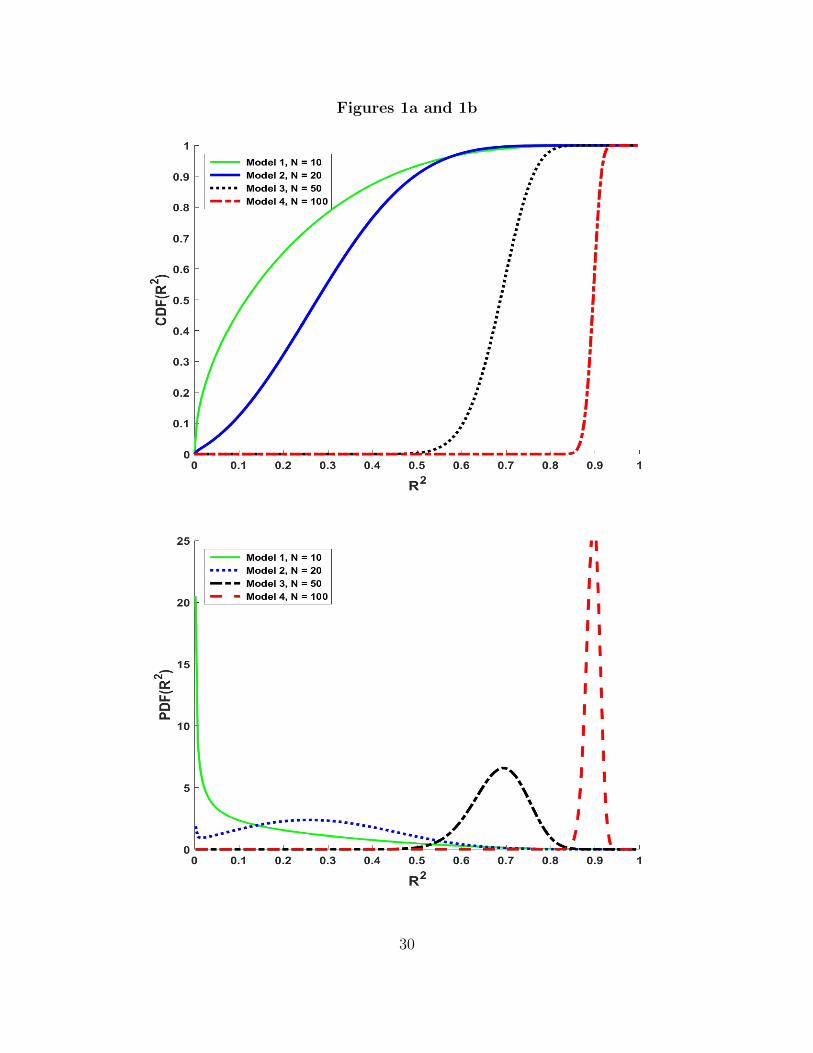
Figures 1 and 2 illustrate how the non-null distribution of R2 depends on the re-

gressors and model parameters. These figures compare the distribution or density

functions for the following models:

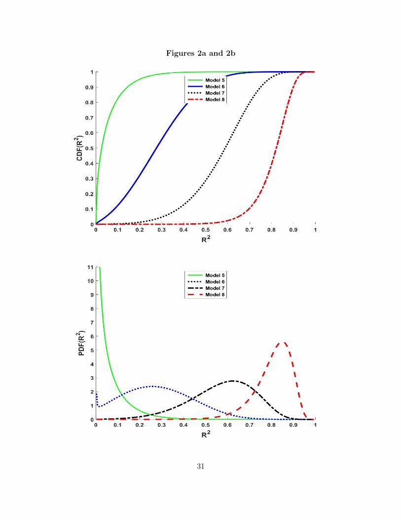
Table 1

Model K T β1 α1 σ2ε σ2

η ∆1 ∆2 θ ρ

1 2 10 0.1 1.0 1.0 0.0 0.835 0.02 2 20 0.1 1.0 1.0 0.0 6.650 0.03 2 50 0.1 1.0 1.0 0.0 104.125 0.04 2 100 0.1 1.0 1.0 0.0 833.250 0.0

5 2 20 0.0 0.1 1.0 0.0 0.000 0.06 2 20 0.1 0.1 1.0 0.0 0.066 0.07 2 20 1.0 0.1 1.0 1.0 6.65 0.508 2 20 1.0 0.1 1.0 4.0 1.66 0.80

In Models 1-4, xi is a deterministic time-trend and the regression R2 has a noncentral

beta distribution. The parameters of the noncentral beta are: 1, N − K, ∆1 =

(β1/σε)2T (T+1)(T−1)/12 and ∆2 = 0. Thus, the numerator noncentrality parameter

increases with the cube of the sample size and the numerator noncentrality parameter

depends on the ratio β1/σε. This ratio measures how fast the mean of y changes

each period relative to the standard deviation of the noise in the time series. If, for

example, β1/σε = 0.1, then it takes 20 periods on average for the conditional mean

14

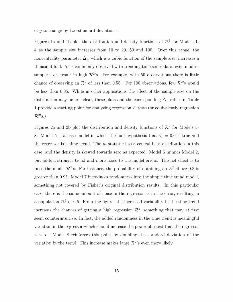
of y to change by two standard deviations.

Figures 1a and 1b plot the distribution and density functions of R2 for Models 1-

4 as the sample size increases from 10 to 20, 50 and 100. Over this range, the

noncentrality parameter ∆1, which is a cubic function of the sample size, increases a

thousand-fold. As is commonly observed with trending time series data, even modest

sample sizes result in high R2’s. For example, with 50 observations there is little

chance of observing an R2 of less than 0.55.. For 100 observations, few R2’s would

be less than 0.85. While in other applications the effect of the sample size on the

distribution may be less clear, these plots and the corresponding ∆1 values in Table

1 provide a starting point for analyzing regression F tests (or equivalently regression

R2’s.)

Figures 2a and 2b plot the distribution and density functions of R2 for Models 5-

8. Model 5 is a base model in which the null hypothesis that β1 = 0.0 is true and

the regressor is a time trend. The m statistic has a central beta distribution in this

case, and the density is skewed towards zero as expected. Model 6 mimics Model 2,

but adds a stronger trend and more noise to the model errors. The net effect is to

raise the model R2’s. For instance, the probability of obtaining an R2 above 0.8 is

greater than 0.95. Model 7 introduces randomness into the simple time trend model,

something not covered by Fisher’s original distribution results. In this particular

case, there is the same amount of noise in the regressor as in the error, resulting in

a population R2 of 0.5. From the figure, the increased variability in the time trend

increases the chances of getting a high regression R2, something that may at first

seem counterintuitive. In fact, the added randomness in the time trend is meaningful

variation in the regressor which should increase the power of a test that the regressor

is zero. Model 8 reinforces this point by doubling the standard deviation of the

variation in the trend. This increase makes large R2’s even more likely.

15

4.2 F Tests and Omitted Variables

The results in the previous subsection focused on singly noncentral or mixtures of

singly noncentral beta or F distributions. This subsection evaluates doubly noncentral

distributions that result from model misspecifications such as omitting regressors.

Specifically, we use the results of Section 2 to study the impact of omitted variables

on the size and power of F tests. While the consequences of omitted variables for

the moments of the least squares coefficient estimates are well understood, their

consequences for significance tests are less well understood. As an example, consider

the extreme case where there are omitted regressors L, and these omitted regressors

are uncorrelated with the included regressors X. In this case, the coefficients on

the included regressors are unbiased, but little attention is given to how the omitted

regressors might affect coefficient inferences. For example, it might seem that because

the estimates of the coefficients are unbiased, that the likelihood of rejecting a correct

null is unaffected. This is not the case.

To illustrate, consider the previous bivariate linear trend regression:

yt = β0 + β1t+ εt.

Suppose that we have incorrectly omitted the single regressor L which is a nonlinear

function of time:

L = γ0t+ γ1 sin(t).

The parameter γ0 affects the correlation between the included time trend and the

excluded variable L, which oscillates with t. The following models examine how the

truth of the null and the correlation of the excluded variable with the included time

trend affect the square of the t statistic on the time trend (which has the Lagrange

multiplier form given in equation (2)). Models 9-12 test the incorrect restriction that

16

β1 = 0.0. The model labelled Null in the last line of the table correctly tests β1 = 0.1.5

Table 2aModel 9-12 Descriptions

Model K T β1 γ0 γ1 σ2ε Corr(t, L) ∆1 ∆2

9 2 20 0.1 0.0 0.00 1.0 – 6.650 0.00010 2 20 0.1 5.0 0.00 1.0 -0.095 1.125 253.87811 2 20 0.1 5.0 0.25 1.0 0.296 56.366 253.87812 2 20 0.1 1.0 0.50 1.0 0.581 194.731 253.878

Null 2 20 0.1 0.0 0.0 1.0 – 0.000 0.000

Table 2bPower Calculations for F-test

Model Acceptance Rates forα = 0.10 α = 0.05 α = 0.01

9 0.201 0.316 0.59210 1.000 1.000 1.00011 0.233 0.718 0.99912 0.000 0.000 0.010

Null 0.900 0.950 0.990

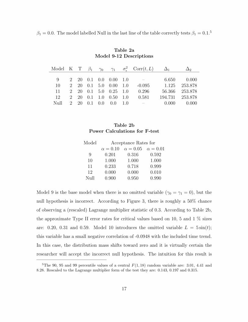
Model 9 is the base model when there is no omitted variable (γ0 = γ1 = 0), but the

null hypothesis is incorrect. According to Figure 3, there is roughly a 50% chance

of observing a (rescaled) Lagrange multiplier statistic of 0.3. According to Table 2b,

the approximate Type II error rates for critical values based on 10, 5 and 1 % sizes

are: 0.20, 0.31 and 0.59. Model 10 introduces the omitted variable L = 5 sin(t);

this variable has a small negative correlation of -0.0948 with the included time trend.

In this case, the distribution mass shifts toward zero and it is virtually certain the

researcher will accept the incorrect null hypothesis. The intuition for this result is

5The 90, 95 and 99 percentile values of a central F (1, 18) random variable are: 3.01, 4.41 and8.28. Rescaled to the Lagrange multiplier form of the test they are: 0.143, 0.197 and 0.315.

17

that the omitted variable inflates the apparent variance of the regression error, which

is reflected in a large denominator noncentrality parameter, ∆2.

Model 11 increases the correlation of the time trend and the omitted variable to 0.296,

while keeping the denominator noncentrality parameter the same as Model 10. This

change shifts the distribution to the right, increasing the power of the test so that the

Type II error rate using a 10 percent critical value is comparable to what it would

be if there were no omitted variable. Model 12 increases the correlation further and

shows that eventually the F test can detect the incorrect null with high probability

despite the pesence of the omitted variable.

4.3 Wu-Hausman-Revenkar Endogeneity Tests

The applied econometrics literature has devoted considerable attention to the problem

of testing whether some right hand side regressors in a linear regression model are

correlated with the equation’s error term. Nakamura and Nakamura (1998) provide

an overview and survey of this topic and discuss popular tests proposed by Wu (1973),

Hausman (1978) and Revenkar (1978). The power of these tests can be an important

issue in finite samples, particularly in cases where the instruments are seen as “weak”.

As with many linear specification tests, the Wu-Hausman-Revenkar (WHR) endo-

geneity test can be implemented via an auxiliary regression (Hausman (1977) and

Davidson and McKinnon (1993)). For example, let the equation of interest be

y1 = X1β1 + Y2β2 + η1 (28)

where the X1 are exogenous variables uncorrelated with η1 and the Y2 are candidate

endogenous variables. Let the candidate endogenous variables have the reduced form

Y2 = X1π21 +X2π22 + V2 = Xπ2 + V2 (29)

where the X2 are potential instruments. Under the endogeneity hypothesis, η1 has

18

the form

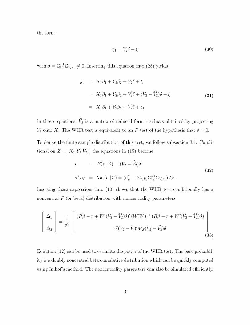
η1 = V2δ + ξ (30)

with δ = Σ−1V2 ΣV2η1 6= 0. Inserting this equation into (28) yields

y1 = X1β1 + Y2β2 + V2δ + ξ

= X1β1 + Y2β2 + V2δ + (V2 − V2)δ + ξ

= X1β1 + Y2β2 + V2δ + ε1

(31)

In these equations, V2 is a matrix of reduced form residuals obtained by projecting

Y2 onto X. The WHR test is equivalent to an F test of the hypothesis that δ = 0.

To derive the finite sample distribution of this test, we follow subsection 3.1. Condi-

tional on Z = [X1 Y2 V2 ], the equations in (15) become

µ = E(ε1|Z) = (V2 − V2)δ

σ2IN = Var(ε1|Z) = (σ2ε1− Σε1V2Σ

−1V2

ΣV2ε1) IN .

(32)

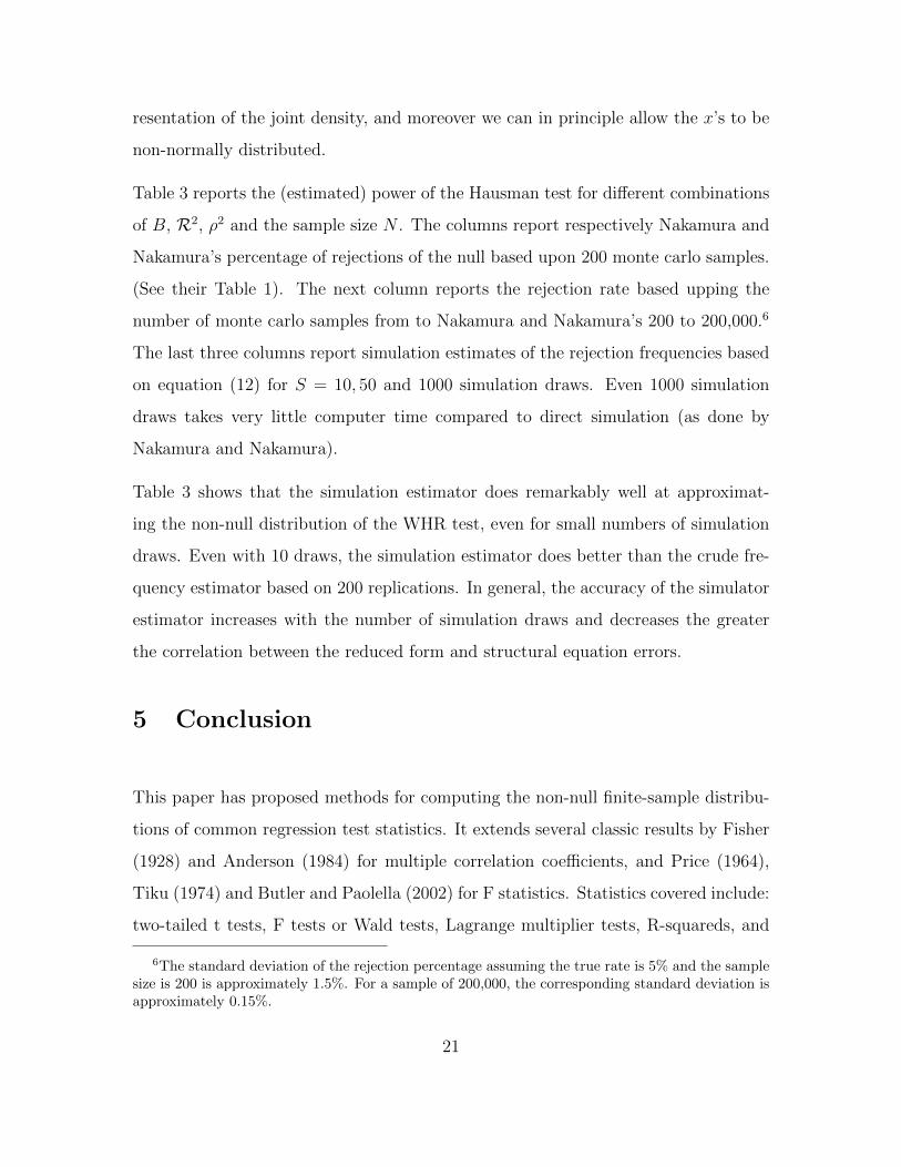
Inserting these expressions into (10) shows that the WHR test conditionally has a

noncentral F (or beta) distribution with noncentrality parameters

∆1

∆2

=1

σ2

(Rβ − r +W ′(V2 − V2)δ)′ (W ′W )−1 (Rβ − r +W ′(V2 − V2)δ)

δ′(V2 − V )′MZ(V2 − V2)δ

(33)

Equation (12) can be used to estimate the power of the WHR test. The base probabil-

ity is a doubly noncentral beta cumulative distribution which can be quickly computed

using Imhof’s method. The noncentrality paraneters can also be simulated efficiently.

19

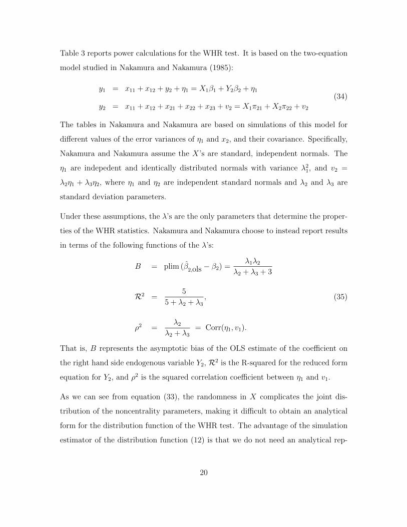
Table 3 reports power calculations for the WHR test. It is based on the two-equation

model studied in Nakamura and Nakamura (1985):

y1 = x11 + x12 + y2 + η1 = X1β1 + Y2β2 + η1

y2 = x11 + x12 + x21 + x22 + x23 + v2 = X1π21 +X2π22 + v2

(34)

The tables in Nakamura and Nakamura are based on simulations of this model for

different values of the error variances of η1 and x2, and their covariance. Specifically,

Nakamura and Nakamura assume the X’s are standard, independent normals. The

η1 are indepedent and identically distributed normals with variance λ21, and v2 =

λ2η1 + λ3η2, where η1 and η2 are independent standard normals and λ2 and λ3 are

standard deviation parameters.

Under these assumptions, the λ’s are the only parameters that determine the proper-

ties of the WHR statistics. Nakamura and Nakamura choose to instead report results

in terms of the following functions of the λ’s:

B = plim (β2,ols − β2) =

λ1λ2λ2 + λ3 + 3

R2 =5

5 + λ2 + λ3,

ρ2 =λ2

λ2 + λ3= Corr(η1, v1).

(35)

That is, B represents the asymptotic bias of the OLS estimate of the coefficient on

the right hand side endogenous variable Y2, R2 is the R-squared for the reduced form

equation for Y2, and ρ2 is the squared correlation coefficient between η1 and v1.

As we can see from equation (33), the randomness in X complicates the joint dis-

tribution of the noncentrality parameters, making it difficult to obtain an analytical

form for the distribution function of the WHR test. The advantage of the simulation

estimator of the distribution function (12) is that we do not need an analytical rep-

20

resentation of the joint density, and moreover we can in principle allow the x’s to be

non-normally distributed.

Table 3 reports the (estimated) power of the Hausman test for different combinations

of B, R2, ρ2 and the sample size N . The columns report respectively Nakamura and

Nakamura’s percentage of rejections of the null based upon 200 monte carlo samples.

(See their Table 1). The next column reports the rejection rate based upping the

number of monte carlo samples from to Nakamura and Nakamura’s 200 to 200,000.6

The last three columns report simulation estimates of the rejection frequencies based

on equation (12) for S = 10, 50 and 1000 simulation draws. Even 1000 simulation

draws takes very little computer time compared to direct simulation (as done by

Nakamura and Nakamura).

Table 3 shows that the simulation estimator does remarkably well at approximat-

ing the non-null distribution of the WHR test, even for small numbers of simulation

draws. Even with 10 draws, the simulation estimator does better than the crude fre-

quency estimator based on 200 replications. In general, the accuracy of the simulator

estimator increases with the number of simulation draws and decreases the greater

the correlation between the reduced form and structural equation errors.

5 Conclusion

This paper has proposed methods for computing the non-null finite-sample distribu-

tions of common regression test statistics. It extends several classic results by Fisher

(1928) and Anderson (1984) for multiple correlation coefficients, and Price (1964),

Tiku (1974) and Butler and Paolella (2002) for F statistics. Statistics covered include:

two-tailed t tests, F tests or Wald tests, Lagrange multiplier tests, R-squareds, and

6The standard deviation of the rejection percentage assuming the true rate is 5% and the samplesize is 200 is approximately 1.5%. For a sample of 200,000, the corresponding standard deviation isapproximately 0.15%.

21

adjusted R-squareds, as well as similar statistics that apply to models with stochas-

tic regressors, such as Wu-Hausman-Revenkar endogeneity tests. The distribution

results cover models with incorrect restrictions and functional forms. In addition to

providing distribution formulae, practical computational algorithms were proposed

and illustrated. The examples included models with trends, omitted variables and

stochastic regressors.

While the results of this paper can be used to understand the consequences of model-

ing choices for test outcomes when the model errors are normally distributed, further

work needs to be done to understand finite sample issues that arise when the errors

are not normally distributed. Some of the results here can be extended to cover more

general error distributions in the elliptical family. Some of the simulation techniques

could also be used to study error distributions composed of mixtures of normals.

These possibilities are being explored in future work.

22

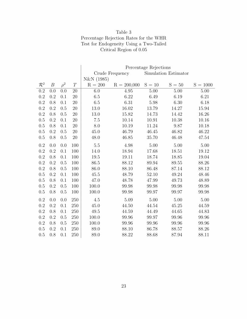
Table 3Percentage Rejection Rates for the WHRTest for Endogeneity Using a Two-Tailed

Critical Region of 0.05

Percentage RejectionsCrude Frequency Simulation Estimator

N&N (1985)R2 B ρ2 T R = 200 R = 200,000 S = 10 S = 50 S = 10000.2 0.0 0.0 20 6.0 4.95 5.00 5.00 5.000.2 0.2 0.1 20 6.5 6.22 6.49 6.19 6.210.2 0.8 0.1 20 6.5 6.31 5.98 6.30 6.180.2 0.2 0.5 20 13.0 16.02 13.79 14.27 15.940.2 0.8 0.5 20 13.0 15.82 14.73 14.42 16.260.5 0.2 0.1 20 7.5 10.14 10.91 10.38 10.160.5 0.8 0.1 20 8.0 10.19 11.24 9.87 10.180.5 0.2 0.5 20 45.0 46.79 46.45 46.82 46.220.5 0.8 0.5 20 48.0 46.85 35.70 46.48 47.54

0.2 0.0 0.0 100 5.5 4.98 5.00 5.00 5.000.2 0.2 0.1 100 14.0 18.94 17.68 18.51 19.120.2 0.8 0.1 100 19.5 19.11 18.74 18.85 19.040.2 0.2 0.5 100 86.5 88.12 89.94 89.55 88.260.2 0.8 0.5 100 86.0 88.10 86.48 87.14 88.120.5 0.2 0.1 100 45.5 48.79 52.10 49.24 48.460.5 0.8 0.1 100 47.0 48.78 47.99 49.73 48.890.5 0.2 0.5 100 100.0 99.98 99.98 99.98 99.980.5 0.8 0.5 100 100.0 99.98 99.97 99.97 99.98

0.2 0.0 0.0 250 4.5 5.09 5.00 5.00 5.000.2 0.2 0.1 250 45.0 44.50 44.54 45.25 44.590.2 0.8 0.1 250 49.5 44.59 44.49 44.65 44.830.2 0.2 0.5 250 100.0 99.96 99.97 99.96 99.960.2 0.8 0.5 250 100.0 99.96 99.96 99.96 99.960.5 0.2 0.1 250 89.0 88.10 86.78 88.57 88.260.5 0.8 0.1 250 89.0 88.22 88.68 87.94 88.11

23

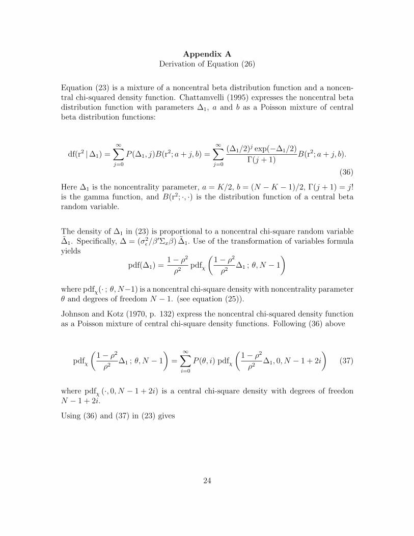
Appendix ADerivation of Equation (26)

Equation (23) is a mixture of a noncentral beta distribution function and a noncen-tral chi-squared density function. Chattamvelli (1995) expresses the noncentral betadistribution function with parameters ∆1, a and b as a Poisson mixture of centralbeta distribution functions:

df(r2 |∆1) =∞∑j=0

P (∆1, j)B(r2; a+ j, b) =∞∑j=0

(∆1/2)j exp(−∆1/2)

Γ(j + 1)B(r2; a+ j, b).

(36)

Here ∆1 is the noncentrality parameter, a = K/2, b = (N −K − 1)/2, Γ(j + 1) = j!is the gamma function, and B(r2; ·, ·) is the distribution function of a central betarandom variable.

The density of ∆1 in (23) is proportional to a noncentral chi-square random variable∆1. Specifically, ∆ = (σ2

ε/β′Σxβ) ∆1. Use of the transformation of variables formula

yields

pdf(∆1) =1− ρ2

ρ2pdfχ

(1− ρ2

ρ2∆1 ; θ,N − 1

)where pdfχ(· ; θ,N−1) is a noncentral chi-square density with noncentrality parameterθ and degrees of freedom N − 1. (see equation (25)).

Johnson and Kotz (1970, p. 132) express the noncentral chi-squared density functionas a Poisson mixture of central chi-square density functions. Following (36) above

pdfχ

(1− ρ2

ρ2∆1 ; θ,N − 1

)=∞∑i=0

P (θ, i) pdfχ

(1− ρ2

ρ2∆1, 0, N − 1 + 2i

)(37)

where pdfχ (·, 0, N − 1 + 2i) is a central chi-square density with degrees of freedonN − 1 + 2i.

Using (36) and (37) in (23) gives

24

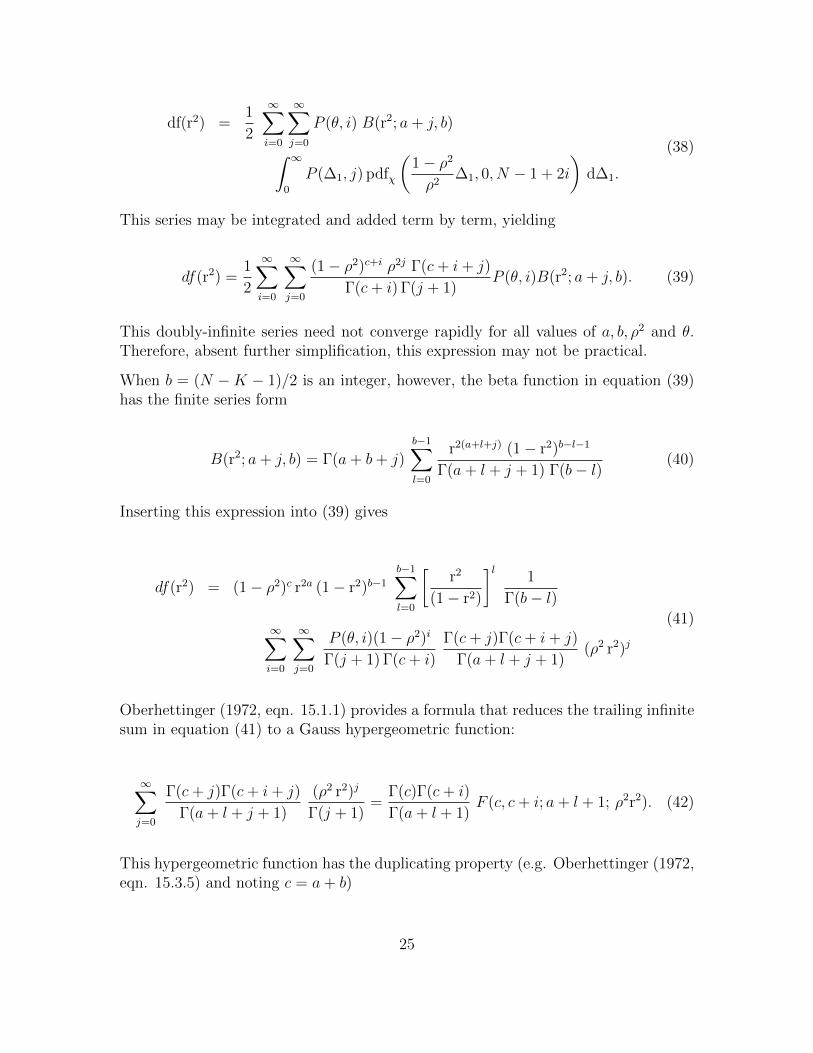
df(r2) =1

2

∞∑i=0

∞∑j=0

P (θ, i) B(r2; a+ j, b)∫ ∞0

P (∆1, j) pdfχ

(1− ρ2

ρ2∆1, 0, N − 1 + 2i

)d∆1.

(38)

This series may be integrated and added term by term, yielding

df(r2) =1

2

∞∑i=0

∞∑j=0

(1− ρ2)c+i ρ2j Γ(c+ i+ j)

Γ(c+ i) Γ(j + 1)P (θ, i)B(r2; a+ j, b). (39)

This doubly-infinite series need not converge rapidly for all values of a, b, ρ2 and θ.Therefore, absent further simplification, this expression may not be practical.

When b = (N −K − 1)/2 is an integer, however, the beta function in equation (39)has the finite series form

B(r2; a+ j, b) = Γ(a+ b+ j)b−1∑l=0

r2(a+l+j) (1− r2)b−l−1

Γ(a+ l + j + 1) Γ(b− l)(40)

Inserting this expression into (39) gives

df(r2) = (1− ρ2)c r2a (1− r2)b−1b−1∑l=0

[r2

(1− r2)

]l1

Γ(b− l)

∞∑i=0

∞∑j=0

P (θ, i)(1− ρ2)i

Γ(j + 1) Γ(c+ i)

Γ(c+ j)Γ(c+ i+ j)

Γ(a+ l + j + 1)(ρ2 r2)j

(41)

Oberhettinger (1972, eqn. 15.1.1) provides a formula that reduces the trailing infinitesum in equation (41) to a Gauss hypergeometric function:

∞∑j=0

Γ(c+ j)Γ(c+ i+ j)

Γ(a+ l + j + 1)

(ρ2 r2)j

Γ(j + 1)=

Γ(c)Γ(c+ i)

Γ(a+ l + 1)F (c, c+ i; a+ l + 1; ρ2r2). (42)

This hypergeometric function has the duplicating property (e.g. Oberhettinger (1972,eqn. 15.3.5) and noting c = a+ b)

25

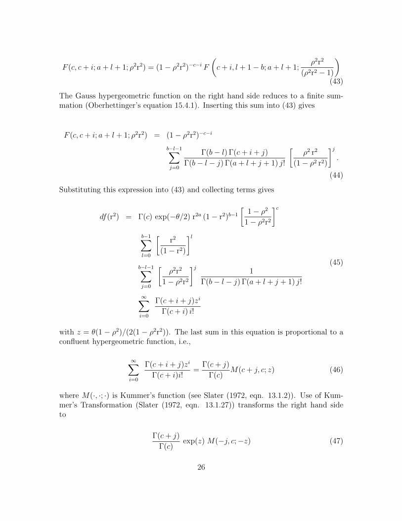
F (c, c+ i; a+ l + 1; ρ2r2) = (1− ρ2r2)−c−i F(c+ i, l + 1− b; a+ l + 1;

ρ2r2

(ρ2r2 − 1)

)(43)

The Gauss hypergeometric function on the right hand side reduces to a finite sum-mation (Oberhettinger’s equation 15.4.1). Inserting this sum into (43) gives

F (c, c+ i; a+ l + 1; ρ2r2) = (1− ρ2r2)−c−i

b−l−1∑j=0

Γ(b− l) Γ(c+ i+ j)

Γ(b− l − j) Γ(a+ l + j + 1) j!

[ρ2 r2

(1− ρ2 r2)

]j.

(44)

Substituting this expression into (43) and collecting terms gives

df(r2) = Γ(c) exp(−θ/2) r2a (1− r2)b−1[

1− ρ2

1− ρ2r2

]cb−1∑l=0

[r2

(1− r2)

]lb−l−1∑j=0

[ρ2r2

1− ρ2r2

]j1

Γ(b− l − j) Γ(a+ l + j + 1) j!

∞∑i=0

Γ(c+ i+ j)zi

Γ(c+ i) i!

(45)

with z = θ(1 − ρ2)/(2(1 − ρ2r2)). The last sum in this equation is proportional to aconfluent hypergeometric function, i.e.,

∞∑i=0

Γ(c+ i+ j)zi

Γ(c+ i)i!=

Γ(c+ j)

Γ(c)M(c+ j, c; z) (46)

where M(·, ·; ·) is Kummer’s function (see Slater (1972, eqn. 13.1.2)). Use of Kum-mer’s Transformation (Slater (1972, eqn. 13.1.27)) transforms the right hand sideto

Γ(c+ j)

Γ(c)exp(z) M(−j, c;−z) (47)

26

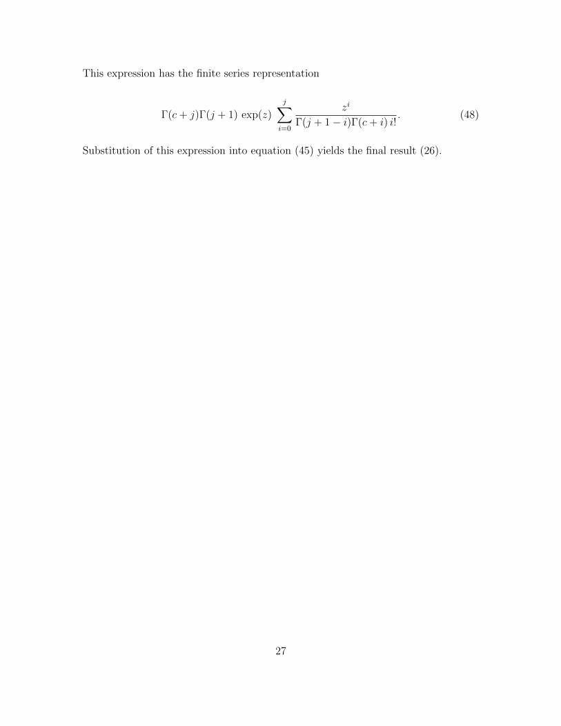
This expression has the finite series representation

Γ(c+ j)Γ(j + 1) exp(z)

j∑i=0

zi

Γ(j + 1− i)Γ(c+ i) i!. (48)

Substitution of this expression into equation (45) yields the final result (26).

27

References

Anderson, T.W. (1984), An Introduction, to Multivariate Statistical Analysis. NewYork: John Wiley & Sons.

Chattamvelli, R. (1995), “A Note on the Noncentral Beta Distribution Function,”The American Statistician 49(2): 231-234

Cohen, J. (1977), Statistical Power Analysis for the Behavioral Sciences. New York:Academic Press.

Davidson, R. and J. MacKinnon (1993), Estimation and Inference in Economet-rics,New York: Oxford University Press

Evans, G.B.A. and N.E. Savin (1982), “Conflict Among the Criteria Revisited: TheW, LR and LM Tests,” Econometrica 50, 737-748.

Fisher, R.A. (1928), “The General Sampling Distribution of the Multiple CorrelationCoefficient,” Proceedings of the Royal Society of London 121 A, 654-673.

Imhof, J.P. (1961), “Computing The Distribution of Quadratic Forms in NormalVariables,” Biometrika 48, 419-426.

Johnson, N.L. and S. Kotz (1970), Continuous Univariate Distributions - 2. NewYork: John Wiley & Sons.

Kennedy, W.E. and J.E. Gentle (1980), Statistical Computing. New York: MarcelDekker.

Koerts, J. and A.P.J. Abrahamse (1969), On The Theory and Application of theGeneral Linear Model. Rotterdam: Universitaire Pers Rotterdam.

Kramer, K.H. (1963), “Tables for Constructing Confidence Limits on the MultipleCorrelation Coefficient,” Journal of the American Statistical Association 58,1082-1085.

Lenth, R.V. (1987), “Algorithm AS 226: Computing Noncentral Beta Probabilities,”Applied Statistics 35, 241-244.

Muirhead, R. (1982), Aspects of Multivariate Statistical Theory. New York: JohnWiley & Sons.

Nakamura, A. and M. Nakamura (1998), “Model specification and endogeneity,”Journal of Econometrics, 83, 213-237.

Nicholson, W.L. (1954), “A Computing Formula for the Power of the Analysis ofVariance Test,” Annals of Mathematical Statistics 25, 607-610.

28

Oberhettinger, F. (1972), “Hypergeometric Functions,” Chapter 15 in M. Abramowitzand I. Stegun eds., Handbook of Mathematical Functions with Formulas, Graphs,and Mathematical Tables, National Bureau of Standards Applied MathematicsSeries: 55, Tenth edition; Washington.

Patnaik, P.B. (1949), “The Noncentral x2 and F Distributions and Their Applica-tions,” Biometrika 36, 202-232.

Phillips, P.C.B. (1986), “The Exact Distribution of the Wald Statistic,” Economet-rica 54, 881-895.

Posten, H. (1993). ”An Effective Algorithm for the Noncentral Beta DistributionFunction”. The American Statistician 47 (2): 129131.

Price, R. (1964), “Some Noncentral F Distributions Expressed in Closed Form,”Biometrika 51, 107-122.

Rao, C.R. (1973), Linear Statistical Inference and its Applications. New York: JohnWiley & Sons.

Reiss, P.C. (2015), Further Distribution Results on Correlation Coefficients in Nor-mal Samples. Stanford Business School Working Paper.

Slater, L.J. (1972), “Confluent Hypergeometric Functions,” Chapter 13 in M. Abramowitzand I. Stegun eds., Handbook of Mathematical Functions with Formulas, Graphs,and Mathematical Tables, National Bureau of Standards Applied MathematicsSeries: 55, Tenth edition; Washington.

Tang, P.C. (1938), “The Power Function of the Analysis of Variance Tests withTables and Illustrations of Their Use,” Statistical Research Memoirs 2, 126-158.

Tiku, M.L. (1967), “Tables of the Power of the F Test,” Journal of the AmericanStatistical Association 62, 525-539.

Tiku, M.L. (1974), Doubly Noncentral F Distribution - Tables and Applications. InH.L. Harter and D.B. Owen eds., Selected Tables in Mathematical Statistics,Volume 2, Providence, R.I.: American Mathematical Society.

Wishart, J. (1932), “A Note on the Distribution of the Correlation Ratio,” Biometrika24, 441-456.

Zelen, M. and N. Severo (1972), “Probability Functions,” Chapter 26 in M. Abramowitzand I. Stegun eds., Handbook of Mathematical Functions, Washington, D.C.:U.S. Department of Commerce.

29

Figures 1a and 1b

30

Figures 2a and 2b

31

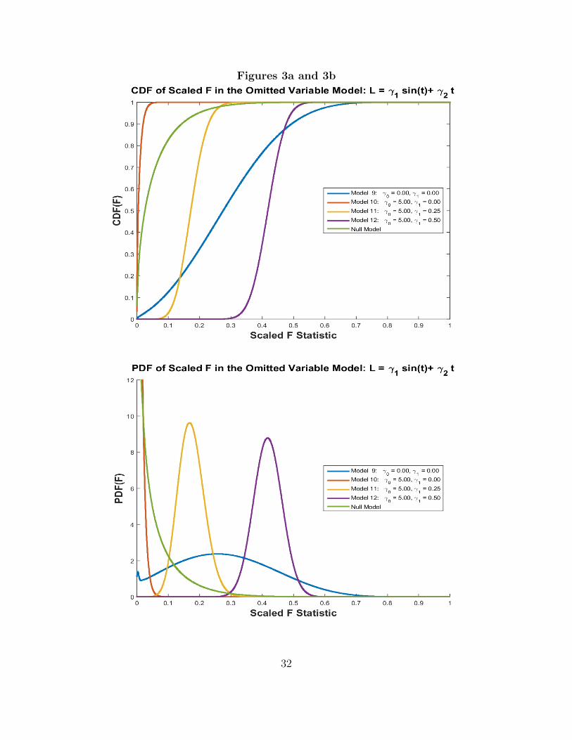
Figures 3a and 3b

32