Finite-Reynolds-numbereﬀectsinturbulence

J. Fluid Mech. (2006), vol. 554, pp. 477–498. c© 2006 Cambridge University Press

doi:10.1017/S002211200600913X Printed in the United Kingdom

477

Finite-Reynolds-number effects in turbulenceusing logarithmic expansions

By K. R. SREENIVASAN1 AND A. BERSHADSKII21The Abdus Salam International Centre for Theoretical Physics, 34014 Trieste, Italy

2ICAR, P.O. Box 31155, Jerusalem 91000, Israel

(Received 4 August 2005 and in revised form 14 January 2006)

Experimental or numerical data in turbulence are invariably obtained at finiteReynolds numbers whereas theories of turbulence correspond to infinitely largeReynolds numbers. A proper merger of the two approaches is possible only ifcorrections for finite Reynolds numbers can be quantified. This paper heuristicallyconsiders examples in two classes of finite-Reynolds-number effects. Expansions interms of logarithms of appropriate variables are shown to yield results in agreementwith experimental and numerical data in the following instances: the third-orderstructure function in isotropic turbulence, the mixed-order structure function for thepassive scalar and the Reynolds shear stress around its maximum point. Resultssuggestive of expansions in terms of the inverse logarithm of the Reynolds number,also motivated by experimental data, concern the tendency for turbulent structuresto cluster along a line of observation and (more speculatively) for the longitudinalvelocity derivative to become singular at some finite Reynolds number. We suggestan elementary hydrodynamical process that may provide a physical basis for theexpansions considered here, but note that the formal justification remains tantalizinglyunclear.

1. IntroductionIf there is a unique state of turbulence at infinitely high Reynolds number, the

question arises as to how to discern its properties from experiments and simulationsat finite Reynolds numbers. The successful history of critical phenomena can bethought to be due to a powerful interplay between experiments on the one handand, on the other hand, theories that accounted for the ‘finite’ effects (such as due tofinite size and finite ‘distances’ away from the critical point). In turbulence, we shouldadmit to knowing no formal way of inferring the right expansions around the infinite-Reynolds-number state, but offer here a few suggestive examples where logarithmicor inverse logarithmic expansions can be given reasonable justification and seem toplay a constructive role – in so far as they allow us to obtain some new results andorganize existing data more systematically. Logarithmic expansions do arise in fieldtheory, and their appropriateness can be established there by partial resummationsbut these tools do not work for turbulence. The only past instances where inverselogarithmic expansions were employed in turbulence seem to be those in Barenblatt(1993), Barenblatt & Goldenfeld (1995), Barenblatt, Chorin & Prostokishin (1997),Castaing, Gagne & Hopfinger (1990) and Dubrulle (1996). We shall not duplicate theexamples that these authors have ably discussed, but examine other instances afterintroducing each of them briefly in the following sections.

478 K. R. Sreenivasan and A. Bershadskii

0

0.2

0.4

0.6

0.8

1.0

log r

–�∆

u3 �/�

ε�r

(i)

(ii)

(iii)

(iv)

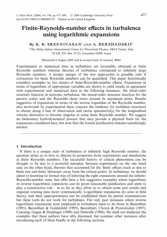
Figure 1. A qualitative sketch of the Kolmogorov function −〈�u3r 〉/〈ε〉r , in terms of the

scale separation r .

The next two sections deal with logarithmic expansions: § 2 considers theKolmogorov and Yaglom laws in isotropic turbulence, while § 3 considers wall-bounded flows. Sections 4 and 5 consider respectively inverse logarithmic expansionsfor the clustering exponents of turbulent structures along an axis of intersection, andfor the flatness factor of velocity derivatives. In each case, results of these expansionsare compared with data from experiments and direct numerical simulations (DNS).Section 6 discusses physical mechanisms in possible support of log-expansions inturbulence.

2. Results for the inertial range of isotropic turbulenceWe restrict attention to stationary isotropic turbulence without concerning ourselves

with the effects of shear, though we expect the results to hold for shear flows as well.

2.1. The Kolmogorov law in isotropic turbulence

The intermediate scales between the large scale L and the dissipation (or Kolmogorov)scale η is called the inertial range. The inertial range of scales is associated with the4/5ths law of Kolmogorov (1941) which states that⟨

�u3r

⟩= − 4

5〈ε〉r. (2.1)

Here, �ur ≡ u(x + r) − u(x) is the longitudinal velocity increment, u is the velocitycomponent in the direction x, and 〈ε〉 is the average of the energy dissipation rate,ε. The Kolmogorov law has a special status in turbulence as it is exact – since it isderived from the Navier–Stokes equations subject only to the asymptotic requirementof ‘sufficiently high’ Reynolds number.

The qualitative behaviour of 〈�u3r 〉, called the third-order structure function, across

the entire range of scales is shown in figure 1. The part labelled (i) is obtained bya Taylor expansion in the limit of r → 0, and that labelled (iii) corresponds to theregion of constant energy flux where the Kolmogorov law is valid. Part (iv) dependson the properties of large scales of the flow. Very little is known about the form of thepart labelled (ii), although there exists an interpolation formula for the corresponding

Logarithmic expansions in turbulence 479

region in even moments (Batchelor 1951; Stolovitzky, Sreenivasan & Juneja 1993).The part (iii) corresponding to (2.1) is expected to appear at high Reynolds numbersand become more extensive with increasing Reynolds number. Experimentally, thereare claims that part (iii) appears even at modest Reynolds numbers but that itsenlargement is very slow in Reynolds number – certainly slower than the growth ofthe ratio between integral and Kolmogorov scales.

To analyse the behaviour at finite Reynolds numbers, consider the Navier–Stokesequations for a viscous incompressible fluid with random force f (x, t), given by

∂ui

∂t+ uj

∂ui

∂xj

= − 1

ρ

∂p

∂xi

+ ν∂2ui

∂x2j

+ fi(x, t), (2.2a)

∂ui

∂xi

= 0, (2.2b)

where ν is kinematic viscosity and ρ is the fluid density. Since the potential part of theexternal force can be included in the pressure gradient, the force can be assumed to besolenoidal. To simplify considerations below, f will be assumed to be Gaussian withzero mean and a rapidly oscillating character, or a δ-correlation in time (Kraichnan1968). Such fields are defined completely by their second-rank correlation tensor

〈fi(x + r, t + τ )fj (x, t)〉Fij (r)δ(τ ). (2.3)

Novikov (1965) used (2.2) and (2.3) to show that the second- and third-orderlongitudinal structure functions are related by the equation

S3 = 6νdS2

dr− 2

r4

∫ r

0

x4Fii(x) dx, (2.4)

where Sn ≡ 〈�unr 〉. Novikov also showed that

Fii(0) = 2〈ε〉. (2.5)

Thus, Fii corresponds to an external energy input rate, an assertion that is alsosupported by Novikov’s relation 〈fi(x, t)vj (x ′, t)〉 = 1

2Fij (x − x ′)).

For r � L, it can be shown readily from (2.4) and (2.5) (see Novikov 1965) that

S3 � 6νdS2

dr− 4

5〈ε〉r. (2.6)

Without the viscous term, this is indeed Kolmogorov’s 4/5ths law. Kolmogorovobtained the result without assumptions on the nature of forcing, but our point isthat the formalism, which we use below, is consistent with the exact result.

Let us rewrite (2.4) formally as

S3 = − 2

r4

∫ r

0

x4F (x) dx, (2.7)

where we define the generalized energy input rate as

F (x) ≡ Fii(x) − 3ν

x4

d(x4dS2/dx)

dx. (2.8)

Assuming the existence of a local maximum of the generalized energy input rate,i.e. a local maximum of F (x) at x = xm (where η < xm < L), let us expand it in termsof the logarithm of the relative distance from xm:

F (x) = F (xm) − a1(ln(x/xm))2 + · · · + an−1(ln(x/xm))n + · · · , (2.9)


1 10 100 10000

0.1

0.2

0.3

0.4

0.5

0.6

0.7

r/η

–�∆

u3 �/�

ε�r

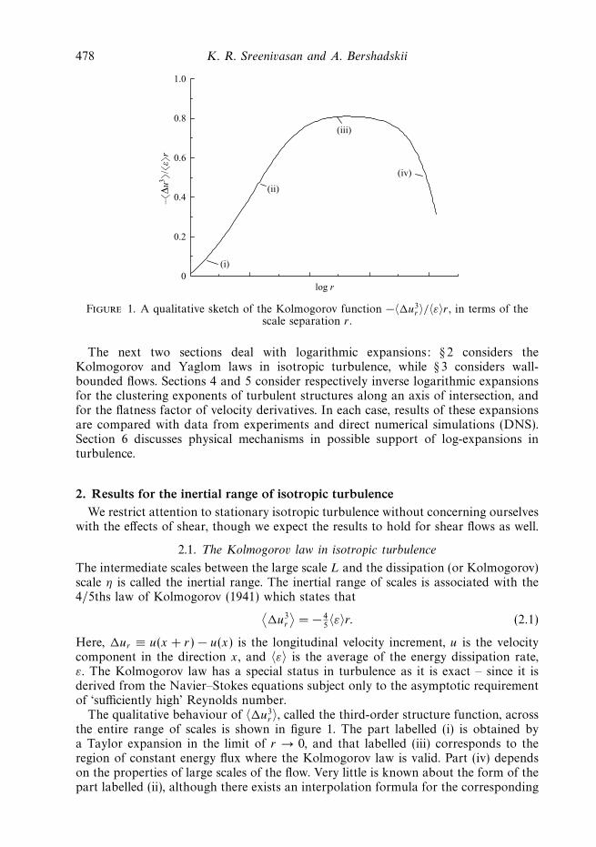
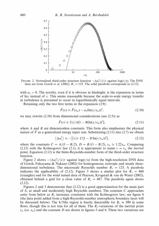
Figure 2. Normalized third-order structure function −�u3r /〈ε〉r against log(r/η). The DNS

data are from Gotoh et al. (2002), Rλ = 125. The solid parabola corresponds to (2.12).

with a1 > 0. The novelty, even if it is obvious in hindsight, is the expansion in termsof lnx instead of x. This seems reasonable because the scale-to-scale energy transferin turbulence is presumed to occur in logarithmically equal intervals.

Retaining only the two first terms in the expansion (2.9):

F (x) � F (xm) − a1(ln(x/xm))2, (2.10)

we may rewrite (2.10) from dimensional considerations (see (2.5)) as

F (x) � 2〈ε〉A[1 − B(ln(x/xm))2], (2.11)

where A and B are dimensionless constants. This form also emphasizes the physicalnature of F as a generalized energy input rate. Substituting (2.11) into (2.7) we obtain⟨

�u3r

⟩� − 4

5〈ε〉r C[1 − D ln(r/rm))2], (2.12)

where the constants C = A/(1 − B/2), D = B/(1 − B/2), rm � 1.22xm. Comparing(2.12) with the Kolmogorov law (2.1), it is appropriate to name r = rm the inertialpoint. Equation (2.12) is the finite-Reynolds-number form of the third-order structurefunction.

Figure 2 shows −〈�u3r 〉/〈ε〉r against log(r/η) from the high-resolution DNS data

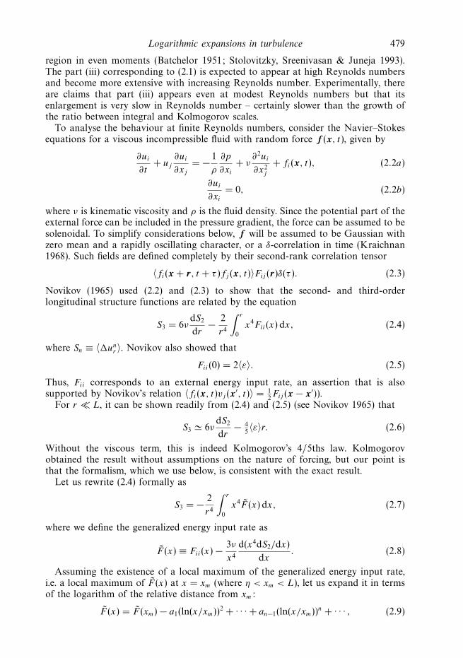
of Gotoh, Fukayama & Nakano (2002) for homogeneous, isotropic and steady three-dimensional turbulence. The microscale Reynolds number Rλ = 125. A parabolaindicates the applicability of (2.12). Figure 3 shows a similar plot for Rλ = 460(triangles) and for the wind tunnel data of Pearson, Krogstad & van de Water (2002),obtained behind a grid for a close value of Rλ = 487. The parabola again shows(2.12).

Figures 2 and 3 demonstrate that (2.12) is a good approximation for the main partof S3 at small and moderately high Reynolds numbers. The constant C approachesunity from below as Rλ increases, consistent with the Kolmogorov law; see figure 4(the data point added from a high-Reynolds-number atmospheric boundary layer willbe discussed below). The 4/5ths region is barely discernible for Rλ ≈ 500 in someflows, though this is not true for all of them. The Rλ-variations of the inertial pointrm (i.e. xm) and the constant D are shown in figures 5 and 6. These two variations are


1 10 100 10000

0.2

0.4

0.6

0.8

r/η

–�∆

u3 �/�

ε�r

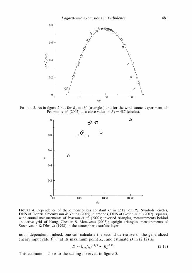
Figure 3. As in figure 2 but for Rλ = 460 (triangles) and for the wind-tunnel experiment ofPearson et al. (2002) at a close value of Rλ = 487 (circles).

10 100 1000 100000

0.2

0.4

0.6

0.8

1.0

Rλ

C

Figure 4. Dependence of the dimensionless constant C in (2.12) on Rλ. Symbols: circles,DNS of Donzis, Sreenivasan & Yeung (2005); diamonds, DNS of Gotoh et al. (2002); squares,wind-tunnel measurements of Pearson et al. (2002); inverted triangles, measurements behindan active grid of Kang, Chester & Meneveau (2003); upright triangles, measurements ofSreenivasan & Dhruva (1998) in the atmospheric surface layer.

not independent. Indeed, one can calculate the second derivative of the generalizedenergy input rate F (x) at its maximum point xm, and estimate D in (2.12) as

D ∼ (rm/η)−4/3 ∼ R−0.97λ . (2.13)

This estimate is close to the scaling observed in figure 5.


10 100 100010

100

1000

Rλ

rm—η

0.73

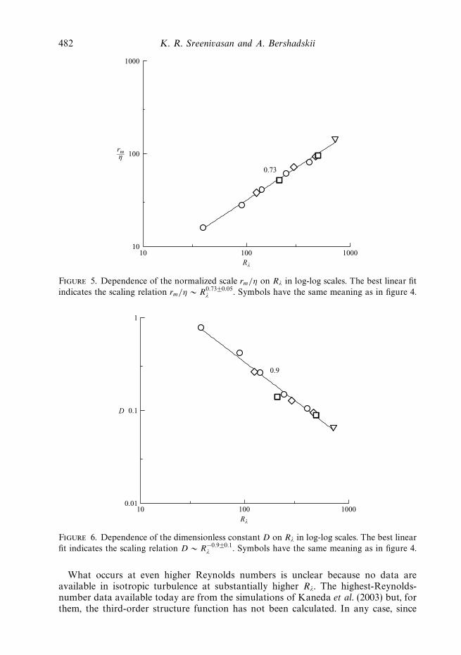
Figure 5. Dependence of the normalized scale rm/η on Rλ in log-log scales. The best linear fit

indicates the scaling relation rm/η ∼ R0.73±0.05λ . Symbols have the same meaning as in figure 4.

10 100 10000.01

0.1

1

Rλ

D

0.9

Figure 6. Dependence of the dimensionless constant D on Rλ in log-log scales. The best linear

fit indicates the scaling relation D ∼ R−0.9±0.1λ . Symbols have the same meaning as in figure 4.

What occurs at even higher Reynolds numbers is unclear because no data areavailable in isotropic turbulence at substantially higher Rλ. The highest-Reynolds-number data available today are from the simulations of Kaneda et al. (2003) but, forthem, the third-order structure function has not been calculated. In any case, since


1 10 100 1000 100000

0.2

0.4

0.6

0.8

1.0

r/η

–�∆

u3 �/�

ε�r

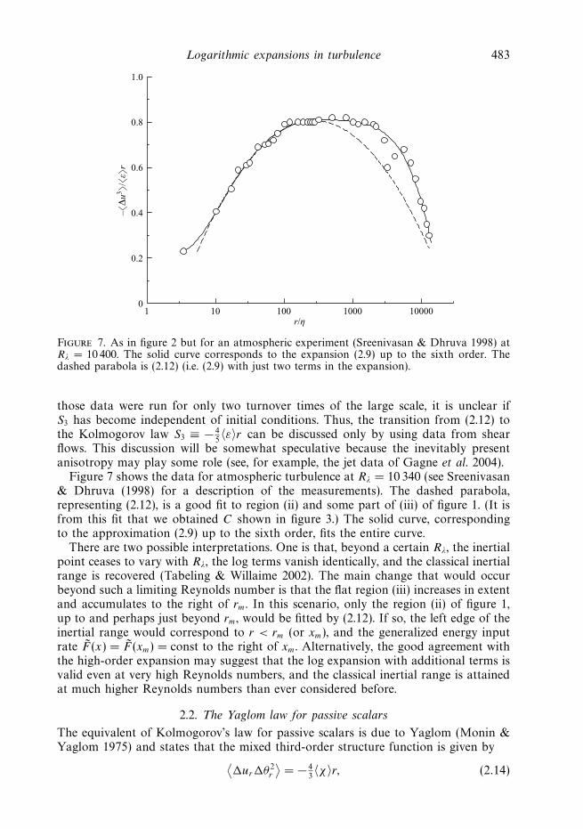
Figure 7. As in figure 2 but for an atmospheric experiment (Sreenivasan & Dhruva 1998) atRλ = 10 400. The solid curve corresponds to the expansion (2.9) up to the sixth order. Thedashed parabola is (2.12) (i.e. (2.9) with just two terms in the expansion).

those data were run for only two turnover times of the large scale, it is unclear ifS3 has become independent of initial conditions. Thus, the transition from (2.12) tothe Kolmogorov law S3 ≡ − 4

5〈ε〉r can be discussed only by using data from shear

flows. This discussion will be somewhat speculative because the inevitably presentanisotropy may play some role (see, for example, the jet data of Gagne et al. 2004).

Figure 7 shows the data for atmospheric turbulence at Rλ = 10 340 (see Sreenivasan& Dhruva (1998) for a description of the measurements). The dashed parabola,representing (2.12), is a good fit to region (ii) and some part of (iii) of figure 1. (It isfrom this fit that we obtained C shown in figure 3.) The solid curve, correspondingto the approximation (2.9) up to the sixth order, fits the entire curve.

There are two possible interpretations. One is that, beyond a certain Rλ, the inertialpoint ceases to vary with Rλ, the log terms vanish identically, and the classical inertialrange is recovered (Tabeling & Willaime 2002). The main change that would occurbeyond such a limiting Reynolds number is that the flat region (iii) increases in extentand accumulates to the right of rm. In this scenario, only the region (ii) of figure 1,up to and perhaps just beyond rm, would be fitted by (2.12). If so, the left edge of theinertial range would correspond to r < rm (or xm), and the generalized energy inputrate F (x) = F (xm) = const to the right of xm. Alternatively, the good agreement withthe high-order expansion may suggest that the log expansion with additional terms isvalid even at very high Reynolds numbers, and the classical inertial range is attainedat much higher Reynolds numbers than ever considered before.

2.2. The Yaglom law for passive scalars

The equivalent of Kolmogorov’s law for passive scalars is due to Yaglom (Monin &Yaglom 1975) and states that the mixed third-order structure function is given by⟨

�ur�θ2r

⟩= − 4

3〈χ〉r, (2.14)


where �θr ≡ θ(x + r) − θ(x) is the increment of the passive scalar θ over a scaleof size r and 〈χ〉 is the average value of the dissipation rate of scalar variance, χ .This formula is valid in the so-called convective range of isotropic turbulence, whichis analogous to the inertial range for hydrodynamic turbulence. The experimentalsituation of this fundamental law is similar to that of the 4/5ths law. On the onehand, indications of this law appear for rather small values of Peclet number. Onthe other hand, formation of the convective (inertial) range itself is quite slow withincreasing Peclet number. Since the qualitative characteristics of the Yaglom law aresimilar to those of Kolmogorov’s, we will be brief in describing overlapping aspects.

The diffusion–convection equation for a passive scalar with random ‘force’ (source)f (x, t) is

∂θ

∂t+ uj

∂θ

∂xj

= κ∂2θ

∂x2j

+ f (x, t), (2.15)

where κ is the molecular diffusivity. As before, we assume Gaussianity and δ-correlation in time for the forcing. The Gaussian forces with zero mean are definedby their second-rank correlation

〈f (x + r, t + τ )f (x, t)〉 = F (r)δ(τ ). (2.16)

It is known that the mixed (longitudinal) structure function of third order

Suθ3 (r) = 〈�ur (�θr )

2〉 (2.17)

is related to the second-order structure function Sθ2 (r) = 〈(�θr )

2〉 by the equation

Suθ3 = 2κ

dSθ2

dr− 2

r2

∫ r

0

x2F (x) dx. (2.18)

Let us rewrite (2.18) formally as

Suθ3 = − 2

r2

∫ r

0

x2F (x) dx, (2.19)

where we define generalized input rate for the variance of the passive scalar as

F (x) ≡(

F (x) − κ

x2

d(x2dSθ

2

/dx

)dx

). (2.20)

Let us now assume the existence of a local maximum of the generalized input rate,i.e. a local maximum of F (x) at x = xm (where η < xm < Lθ , η being the moleculardiffusion scale and Lθ the integral scale). From dimensional considerations

F (x) = χψ(x/xm) (2.21)

where ψ(x/xm) is a dimensionless function. The inertial (convective) range is expectedto appear in the flow for sufficiently large Peclet numbers (Monin & Yaglom 1975).We assume that ψ(x/xm) = ψ(1) = const in this range and that, for r within thatrange, this particular value of ψ gives the main contribution to the integral (2.19).From (2.19) follows the result that

Suθ3 (r) = − 2

3χψ(1)r. (2.22)

Taking into account the Yaglom law (2.14) for the convective range, we obtain

ψ(1) = 2. (2.23)


1 10000

0.2

0.4

0.6

0.8

1.0

1.2

1.4

r/η

–�∆

u∆θ

2 �/�

χ�

r

10 100

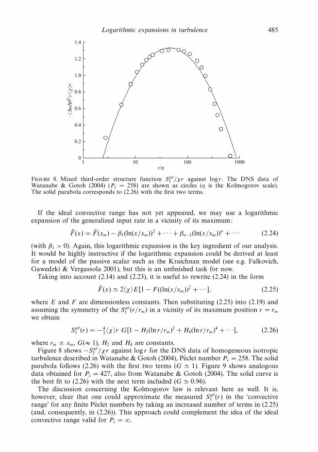
Figure 8. Mixed third-order structure function Suθ3 /χr against log r . The DNS data of

Watanabe & Gotoh (2004) (Pλ = 258) are shown as circles (η is the Kolmogorov scale).The solid parabola corresponds to (2.26) with the first two terms.

If the ideal convective range has not yet appeared, we may use a logarithmicexpansion of the generalized input rate in a vicinity of its maximum:

F (x) = F (xm) − β1(ln(x/xm))2 + · · · + βn−1(ln(x/xm))n + · · · (2.24)

(with β1 > 0). Again, this logarithmic expansion is the key ingredient of our analysis.It would be highly instructive if the logarithmic expansion could be derived at leastfor a model of the passive scalar such as the Kraichnan model (see e.g. Falkovich,Gawedzki & Vergassola 2001), but this is an unfinished task for now.

Taking into account (2.14) and (2.23), it is useful to rewrite (2.24) in the form

F (x) � 2〈χ〉E[1 − F ((ln(x/xm))2 + · · ·], (2.25)

where E and F are dimensionless constants. Then substituting (2.25) into (2.19) andassuming the symmetry of the Suθ

3 (r/rm) in a vicinity of its maximum position r = rm

we obtain

Suθ3 (r) = − 4

3〈χ〉r G[1 − H2(ln r/rm)2 + H4(ln r/rm)4 + · · ·], (2.26)

where rm ∝ xm, G(≈ 1), H2 and H4 are constants.Figure 8 shows −Suθ

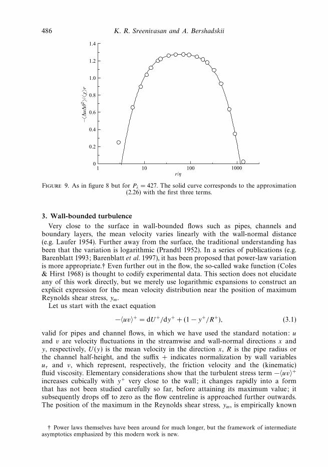
3 /χr against log r for the DNS data of homogeneous isotropicturbulence described in Watanabe & Gotoh (2004), Peclet number Pλ = 258. The solidparabola follows (2.26) with the first two terms (G � 1). Figure 9 shows analogousdata obtained for Pλ = 427, also from Watanabe & Gotoh (2004). The solid curve isthe best fit to (2.26) with the next term included (G � 0.96).

The discussion concerning the Kolmogorov law is relevant here as well. It is,however, clear that one could approximate the measured Suθ

3 (r) in the ‘convectiverange’ for any finite Peclet numbers by taking an increased number of terms in (2.25)(and, consequently, in (2.26)). This approach could complement the idea of the idealconvective range valid for Pλ = ∞.


1 10000

0.2

0.4

0.6

0.8

1.0

1.2

1.4

r/η

–�∆

u∆θ

2 �/�

χ�

r

10 100

Figure 9. As in figure 8 but for Pλ = 427. The solid curve corresponds to the approximation(2.26) with the first three terms.

3. Wall-bounded turbulenceVery close to the surface in wall-bounded flows such as pipes, channels and

boundary layers, the mean velocity varies linearly with the wall-normal distance(e.g. Laufer 1954). Further away from the surface, the traditional understanding hasbeen that the variation is logarithmic (Prandtl 1952). In a series of publications (e.g.Barenblatt 1993; Barenblatt et al. 1997), it has been proposed that power-law variationis more appropriate.† Even further out in the flow, the so-called wake function (Coles& Hirst 1968) is thought to codify experimental data. This section does not elucidateany of this work directly, but we merely use logarithmic expansions to construct anexplicit expression for the mean velocity distribution near the position of maximumReynolds shear stress, ym.

Let us start with the exact equation

−〈uv〉+ = dU+/dy+ + (1 − y+/R+), (3.1)

valid for pipes and channel flows, in which we have used the standard notation: u

and v are velocity fluctuations in the streamwise and wall-normal directions x andy, respectively, U (y) is the mean velocity in the direction x, R is the pipe radius orthe channel half-height, and the suffix + indicates normalization by wall variablesuτ and ν, which represent, respectively, the friction velocity and the (kinematic)fluid viscosity. Elementary considerations show that the turbulent stress term −〈uv〉+

increases cubically with y+ very close to the wall; it changes rapidly into a formthat has not been studied carefully so far, before attaining its maximum value; itsubsequently drops off to zero as the flow centreline is approached further outwards.The position of the maximum in the Reynolds shear stress, ym, is empirically known

† Power laws themselves have been around for much longer, but the framework of intermediateasymptotics emphasized by this modern work is new.


1 10 1000

0.1

0.2

0.3

0.4

0.5

0.6

0.7Re = 3220

Re = 4586

1 10 1000

0.2

0.4

0.6

0.8

1.0

0

0.2

0.4

0.6

0.8

1.0

y+ y+

–�u+v+

�–�

u+v+

�

Re = 10039

1 10 100 1000

Re = 13925

1 10 1000

0.1

0.2

0.3

0.4

0.5

0.6

0.7

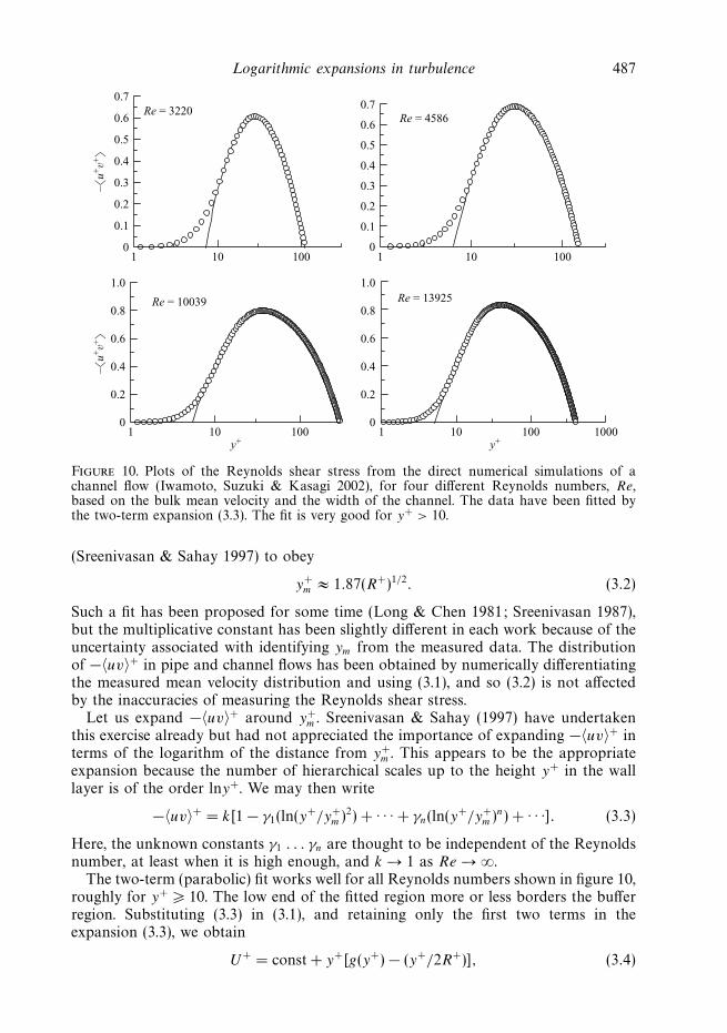
Figure 10. Plots of the Reynolds shear stress from the direct numerical simulations of achannel flow (Iwamoto, Suzuki & Kasagi 2002), for four different Reynolds numbers, Re,based on the bulk mean velocity and the width of the channel. The data have been fitted bythe two-term expansion (3.3). The fit is very good for y+ > 10.

(Sreenivasan & Sahay 1997) to obey

y+m ≈ 1.87(R+)1/2. (3.2)

Such a fit has been proposed for some time (Long & Chen 1981; Sreenivasan 1987),but the multiplicative constant has been slightly different in each work because of theuncertainty associated with identifying ym from the measured data. The distributionof −〈uv〉+ in pipe and channel flows has been obtained by numerically differentiatingthe measured mean velocity distribution and using (3.1), and so (3.2) is not affectedby the inaccuracies of measuring the Reynolds shear stress.

Let us expand −〈uv〉+ around y+m . Sreenivasan & Sahay (1997) have undertaken

this exercise already but had not appreciated the importance of expanding −〈uv〉+ interms of the logarithm of the distance from y+

m . This appears to be the appropriateexpansion because the number of hierarchical scales up to the height y+ in the walllayer is of the order lny+. We may then write

−〈uv〉+ = k[1 − γ1(ln(y+/y+m )2) + · · · + γn(ln(y+/y+

m )n) + · · ·]. (3.3)

Here, the unknown constants γ1 . . . γn are thought to be independent of the Reynoldsnumber, at least when it is high enough, and k → 1 as Re → ∞.

The two-term (parabolic) fit works well for all Reynolds numbers shown in figure 10,roughly for y+ � 10. The low end of the fitted region more or less borders the bufferregion. Substituting (3.3) in (3.1), and retaining only the first two terms in theexpansion (3.3), we obtain

U+ = const + y+[g(y+) − (y+/2R+)], (3.4)


1 10 100 1000 100000

0.2

0.4

0.6

0.8

1.0

y+

(U+/y

+)

+ (

y+/d

+)

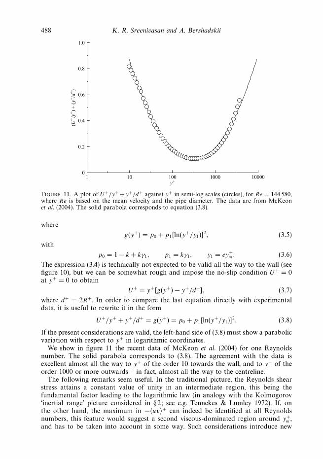
Figure 11. A plot of U+/y+ +y+/d+ against y+ in semi-log scales (circles), for Re = 144 580,where Re is based on the mean velocity and the pipe diameter. The data are from McKeonet al. (2004). The solid parabola corresponds to equation (3.8).

where

g(y+) = p0 + p1[ln(y+/y1)]2, (3.5)

with

p0 = 1 − k + kγ1, p1 = kγ1, y1 = ey+m. (3.6)

The expression (3.4) is technically not expected to be valid all the way to the wall (seefigure 10), but we can be somewhat rough and impose the no-slip condition U+ = 0at y+ = 0 to obtain

U+ = y+[g(y+) − y+/d+], (3.7)

where d+ = 2R+. In order to compare the last equation directly with experimentaldata, it is useful to rewrite it in the form

U+/y+ + y+/d+ = g(y+) = p0 + p1[ln(y+/y1)]2. (3.8)

If the present considerations are valid, the left-hand side of (3.8) must show a parabolicvariation with respect to y+ in logarithmic coordinates.

We show in figure 11 the recent data of McKeon et al. (2004) for one Reynoldsnumber. The solid parabola corresponds to (3.8). The agreement with the data isexcellent almost all the way to y+ of the order 10 towards the wall, and to y+ of theorder 1000 or more outwards – in fact, almost all the way to the centreline.

The following remarks seem useful. In the traditional picture, the Reynolds shearstress attains a constant value of unity in an intermediate region, this being thefundamental factor leading to the logarithmic law (in analogy with the Kolmogorov‘inertial range’ picture considered in § 2; see e.g. Tennekes & Lumley 1972). If, onthe other hand, the maximum in −〈uv〉+ can indeed be identified at all Reynoldsnumbers, this feature would suggest a second viscous-dominated region around y+

m ,and has to be taken into account in some way. Such considerations introduce new


elements in the asymptotic analysis of the wall-bounded flows, and were the subject ofSreenivasan & Sahay (1997). Alternatively, it is possible that the relation (3.2) holdsonly for ‘low’ Reynolds numbers in which case the present considerations hold onlythat range of Reynolds numbers. It is possible that y+

m remains fixed beyond a certainReynolds number so the major influence of increasing the Reynolds number furtheris simply to fill up more and more of the flat part of the Reynolds stress to the rightof y+

m . At present, we do not have sufficiently good data to choose one scenario overthe other.

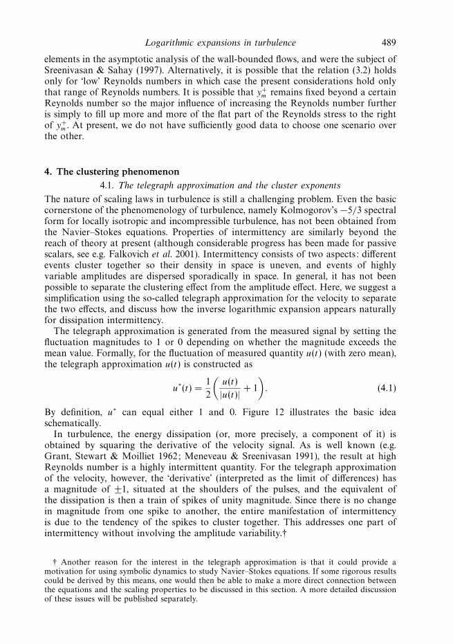
4. The clustering phenomenon4.1. The telegraph approximation and the cluster exponents

The nature of scaling laws in turbulence is still a challenging problem. Even the basiccornerstone of the phenomenology of turbulence, namely Kolmogorov’s −5/3 spectralform for locally isotropic and incompressible turbulence, has not been obtained fromthe Navier–Stokes equations. Properties of intermittency are similarly beyond thereach of theory at present (although considerable progress has been made for passivescalars, see e.g. Falkovich et al. 2001). Intermittency consists of two aspects: differentevents cluster together so their density in space is uneven, and events of highlyvariable amplitudes are dispersed sporadically in space. In general, it has not beenpossible to separate the clustering effect from the amplitude effect. Here, we suggest asimplification using the so-called telegraph approximation for the velocity to separatethe two effects, and discuss how the inverse logarithmic expansion appears naturallyfor dissipation intermittency.

The telegraph approximation is generated from the measured signal by setting thefluctuation magnitudes to 1 or 0 depending on whether the magnitude exceeds themean value. Formally, for the fluctuation of measured quantity u(t) (with zero mean),the telegraph approximation u(t) is constructed as

u∗(t) =1

2

(u(t)

|u(t)| + 1

). (4.1)

By definition, u∗ can equal either 1 and 0. Figure 12 illustrates the basic ideaschematically.

In turbulence, the energy dissipation (or, more precisely, a component of it) isobtained by squaring the derivative of the velocity signal. As is well known (e.g.Grant, Stewart & Moilliet 1962; Meneveau & Sreenivasan 1991), the result at highReynolds number is a highly intermittent quantity. For the telegraph approximationof the velocity, however, the ‘derivative’ (interpreted as the limit of differences) hasa magnitude of ±1, situated at the shoulders of the pulses, and the equivalent ofthe dissipation is then a train of spikes of unity magnitude. Since there is no changein magnitude from one spike to another, the entire manifestation of intermittencyis due to the tendency of the spikes to cluster together. This addresses one part ofintermittency without involving the amplitude variability.†

† Another reason for the interest in the telegraph approximation is that it could provide amotivation for using symbolic dynamics to study Navier–Stokes equations. If some rigorous resultscould be derived by this means, one would then be able to make a more direct connection betweenthe equations and the scaling properties to be discussed in this section. A more detailed discussionof these issues will be published separately.


0

1

u* (t)

–1

0

1

t

∆u* /∆

tu(

t)

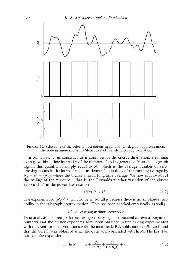
Figure 12. Schematic of the velocity fluctuations signal and its telegraph approximation.The bottom figure shows the ‘derivative’ of the telegraph approximation.

In particular, let us construct, as is common for the energy dissipation, a runningaverage within a time interval τ of the number of spikes generated from the telegraphsignal; this quantity is simply equal to Nτ , which is the average number of zero-crossing points in the interval τ . Let us denote fluctuations of the running average byN ′

τ = Nτ − 〈Nτ 〉, where the brackets mean long-time average. We now inquire aboutthe scaling of the variance – that is, the Reynolds-number variation of the clusterexponent µ∗ in the power-law relation

〈N ′2τ 〉1/2 ∼ τµ∗

. (4.2)

The exponents for 〈N ′qτ 〉1/q will also be µ∗ for all q because there is no amplitude vari-

ability in the telegraph approximation. (This has been checked empirically as well.)

4.2. Inverse logarithmic expansion

Data analysis has been performed using velocity signals measured at several Reynoldsnumbers and the cluster exponents have been obtained. After having experimentedwith different forms of variations with the microscale Reynolds number Rλ, we foundthat the best fit was obtained when the data were correlated with ln Rλ. The first twoterms in the expansion

µ∗(ln Rλ) = q0 +q1

lnRλ

+q2

(lnRλ)2+ · · · (4.3)


0.05 0.10 0.15 0.200

0.1

0.2

0.3

0.4

1/ln (Rλ)

µ*

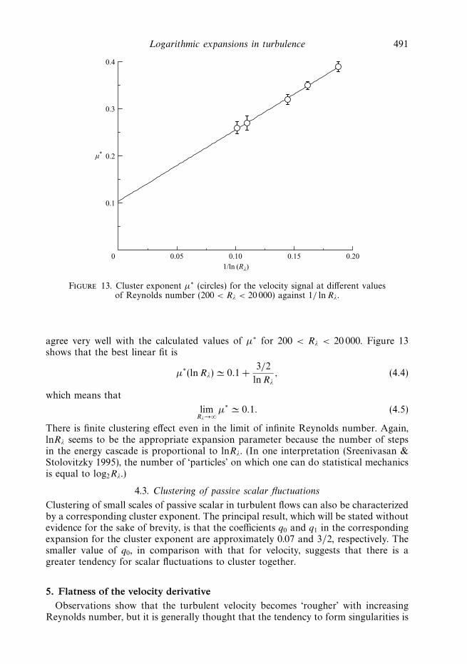
Figure 13. Cluster exponent µ∗ (circles) for the velocity signal at different valuesof Reynolds number (200 < Rλ < 20 000) against 1/ ln Rλ.

agree very well with the calculated values of µ∗ for 200 < Rλ < 20 000. Figure 13shows that the best linear fit is

µ∗(ln Rλ) � 0.1 +3/2

lnRλ

, (4.4)

which means that

limRλ→∞

µ∗ � 0.1. (4.5)

There is finite clustering effect even in the limit of infinite Reynolds number. Again,lnRλ seems to be the appropriate expansion parameter because the number of stepsin the energy cascade is proportional to lnRλ. (In one interpretation (Sreenivasan &Stolovitzky 1995), the number of ‘particles’ on which one can do statistical mechanicsis equal to log2Rλ.)

4.3. Clustering of passive scalar fluctuations

Clustering of small scales of passive scalar in turbulent flows can also be characterizedby a corresponding cluster exponent. The principal result, which will be stated withoutevidence for the sake of brevity, is that the coefficients q0 and q1 in the correspondingexpansion for the cluster exponent are approximately 0.07 and 3/2, respectively. Thesmaller value of q0, in comparison with that for velocity, suggests that there is agreater tendency for scalar fluctuations to cluster together.

5. Flatness of the velocity derivativeObservations show that the turbulent velocity becomes ‘rougher’ with increasing

Reynolds number, but it is generally thought that the tendency to form singularities is


0.1 0.2 0.3 0.4 0.50

0.05

0.10

0.15

0.20

0.25

0.30

0.35

1/ln(Rλ)

F–1

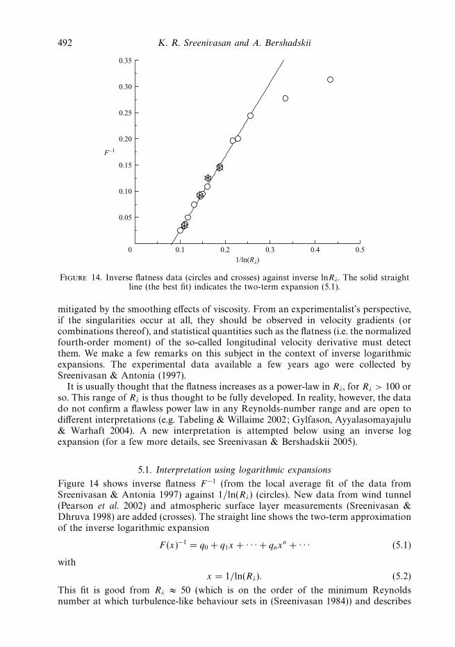
Figure 14. Inverse flatness data (circles and crosses) against inverse lnRλ. The solid straightline (the best fit) indicates the two-term expansion (5.1).

mitigated by the smoothing effects of viscosity. From an experimentalist’s perspective,if the singularities occur at all, they should be observed in velocity gradients (orcombinations thereof), and statistical quantities such as the flatness (i.e. the normalizedfourth-order moment) of the so-called longitudinal velocity derivative must detectthem. We make a few remarks on this subject in the context of inverse logarithmicexpansions. The experimental data available a few years ago were collected bySreenivasan & Antonia (1997).

It is usually thought that the flatness increases as a power-law in Rλ, for Rλ > 100 orso. This range of Rλ is thus thought to be fully developed. In reality, however, the datado not confirm a flawless power law in any Reynolds-number range and are open todifferent interpretations (e.g. Tabeling & Willaime 2002; Gylfason, Ayyalasomayajulu& Warhaft 2004). A new interpretation is attempted below using an inverse logexpansion (for a few more details, see Sreenivasan & Bershadskii 2005).

5.1. Interpretation using logarithmic expansions

Figure 14 shows inverse flatness F −1 (from the local average fit of the data fromSreenivasan & Antonia 1997) against 1/ln(Rλ) (circles). New data from wind tunnel(Pearson et al. 2002) and atmospheric surface layer measurements (Sreenivasan &Dhruva 1998) are added (crosses). The straight line shows the two-term approximationof the inverse logarithmic expansion

F (x)−1 = q0 + q1x + · · · + qnxn + · · · (5.1)

with

x = 1/ln(Rλ). (5.2)

This fit is good from Rλ ≈ 50 (which is on the order of the minimum Reynoldsnumber at which turbulence-like behaviour sets in (Sreenivasan 1984)) and describes


2 8 10 120

1

2

3

4

5

ln(Rλ)

ln(F)

4 6

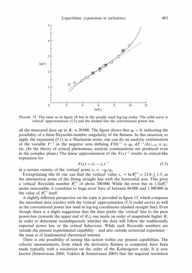
Figure 15. The same as in figure 14 but in the usually used log-log scales. The solid curve is‘critical’ approximation (5.3) and the dashed line the conventional power law.

all the measured data up to Rλ ≈ 20 000. The figure shows that q0 < 0, indicating thepossibility of a finite-Reynolds-number singularity of the flatness. In this situation, toapply the expansion (5.1) as a Maclaurin series, one can do an analytic continuationof the variable F −1 in the negative area defining F (0)−1 ≡ q0, dF −1/dx|x=0 ≡ q1,etc. (In the theory of critical phenomena, analytic continuations are produced evenin the complex plane.) The linear approximation of the F (x)−1 results in critical-likeexpression for

F (x) ∼ (x − xc)−1 (5.3)

in a certain vicinity of the ‘critical’ point xc = −q0/q1.Extrapolating this fit one can find the ‘critical’ value xc = lnR

(c)λ � 12.6 ± 1.5, as

the intersection point of the fitting straight line with the horizontal axis. This givesa ‘critical’ Reynolds number R

(c)λ of about 300 000. While the error bar in 1/lnR

(c)λ

seems reasonable, it translates to huge error bars of between 66 000 and 1 300 000 inthe value of R

(c)λ itself.

A slightly different perspective on the topic is provided in figure 15, which comparesthe smoothed data (circles) with the ‘critical’ approximation (5.3) (solid curve) as wellas the conventional power law used in log-log coordinates (dashed straight line). Eventhough there is a slight suggestion that the data prefer the ‘critical’ line to the purepower-law (towards the upper end of Rλ), one needs an order of magnitude higher Rλ

in order to determine unambiguously whether the data will follow the traditionallyexpected power law or the critical behaviour. While such Reynolds numbers areoutside the present experimental capability – and also outside terrestrial experience –the issue is of fundamental theoretical interest.

There is one possibility of testing this notion within our present capabilities. Thevelocity measurements, from which the derivative flatness is computed, have beenmade typically with a resolution on the order of the Kolmogorov scale. It is nowknown (Sreenivasan 2004; Yakhot & Sreenivasan 2005) that the required resolution


η

κV

2λ

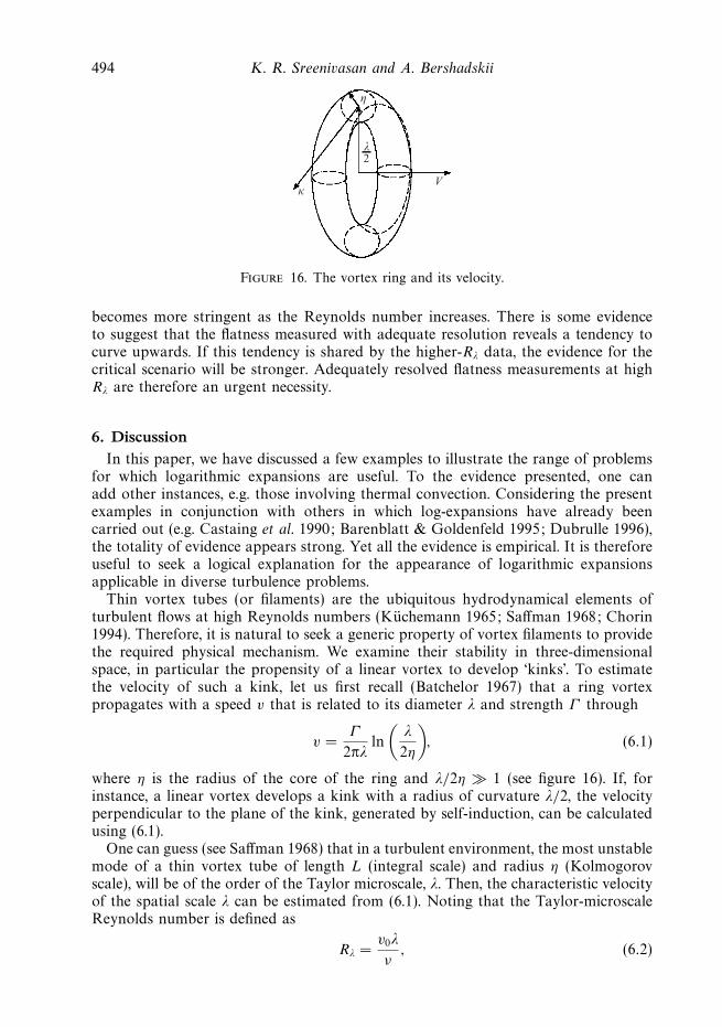
Figure 16. The vortex ring and its velocity.

becomes more stringent as the Reynolds number increases. There is some evidenceto suggest that the flatness measured with adequate resolution reveals a tendency tocurve upwards. If this tendency is shared by the higher-Rλ data, the evidence for thecritical scenario will be stronger. Adequately resolved flatness measurements at highRλ are therefore an urgent necessity.

6. DiscussionIn this paper, we have discussed a few examples to illustrate the range of problems

for which logarithmic expansions are useful. To the evidence presented, one canadd other instances, e.g. those involving thermal convection. Considering the presentexamples in conjunction with others in which log-expansions have already beencarried out (e.g. Castaing et al. 1990; Barenblatt & Goldenfeld 1995; Dubrulle 1996),the totality of evidence appears strong. Yet all the evidence is empirical. It is thereforeuseful to seek a logical explanation for the appearance of logarithmic expansionsapplicable in diverse turbulence problems.

Thin vortex tubes (or filaments) are the ubiquitous hydrodynamical elements ofturbulent flows at high Reynolds numbers (Kuchemann 1965; Saffman 1968; Chorin1994). Therefore, it is natural to seek a generic property of vortex filaments to providethe required physical mechanism. We examine their stability in three-dimensionalspace, in particular the propensity of a linear vortex to develop ‘kinks’. To estimatethe velocity of such a kink, let us first recall (Batchelor 1967) that a ring vortexpropagates with a speed v that is related to its diameter λ and strength Γ through

v =Γ

2πλln

(λ

2η

), (6.1)

where η is the radius of the core of the ring and λ/2η � 1 (see figure 16). If, forinstance, a linear vortex develops a kink with a radius of curvature λ/2, the velocityperpendicular to the plane of the kink, generated by self-induction, can be calculatedusing (6.1).

One can guess (see Saffman 1968) that in a turbulent environment, the most unstablemode of a thin vortex tube of length L (integral scale) and radius η (Kolmogorovscale), will be of the order of the Taylor microscale, λ. Then, the characteristic velocityof the spatial scale λ can be estimated from (6.1). Noting that the Taylor-microscaleReynolds number is defined as

Rλ =v0λ

ν, (6.2)


r

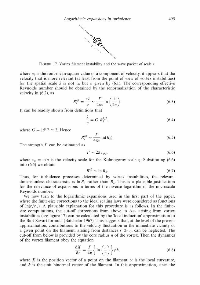
Figure 17. Vortex filament instability and the wave packet of scale r .

where v0 is the root-mean-square value of a component of velocity, it appears that thevelocity that is more relevant (at least from the point of view of vortex instabilities)for the spatial scale λ is not v0 but v given by (6.1). The corresponding effectiveReynolds number should be obtained by the renormalization of the characteristicvelocity in (6.2), as

Reffλ =

vλ

ν∼ Γ

2πνln

(λ

2η

). (6.3)

It can be readily shown from definitions that

λ

η= G R

1/2λ , (6.4)

where G = 151/4 � 2. Hence

Reffλ ∼ Γ

4πνln(Rλ). (6.5)

The strength Γ can be estimated as

Γ ∼ 2πvηη, (6.6)

where vη = ν/η is the velocity scale for the Kolmogorov scale η. Substituting (6.6)into (6.5) we obtain

Reffλ ∼ lnRλ. (6.7)

Thus, for turbulence processes determined by vortex instabilities, the relevantdimensionless characteristic is ln Rλ rather than Rλ. This is a plausible justificationfor the relevance of expansions in terms of the inverse logarithm of the microscaleReynolds number.

We now turn to the logarithmic expansions used in the first part of the paper,where the finite-size corrections to the ideal scaling laws were considered as functionsof ln(r/rm). A plausible explanation for this procedure is as follows. In the finite-size computations, the cut-off corrections from above to �ur arising from vortexinstabilities (see figure 17) can be calculated by the ‘local induction’ approximation tothe Biot-Savart formula (Batchelor 1967). This suggests that, at the level of the presentapproximation, contributions to the velocity fluctuation in the immediate vicinity ofa given point on the filament, arising from distances r � η, can be neglected. Thecut-off from below is provided by the core radius η of the vortex. Then the dynamicsof the vortex filament obey the equation

dXdt

=Γ

4π

{ln

(r

η

)}γ b, (6.8)

where X is the position vector of a point on the filament, γ is the local curvature,and b is the unit binormal vector of the filament. In this approximation, since the


dependence on r is exclusively determined by the logarithmic term in the right-handside of (6.8), a correction function to the turbulent velocity fluctuations, related to thefinite-size effects, is also a function of ln(r/η).

Let us now consider a finite-size correction function f (ln(r/η)) with its maximum atr = rm (see § 2). This function can be rewritten as f (ln(r/η)) ≡ f (ln(r/rm)+ ln(rm/η)).In the vicinity of the maximum, we have

lnrm

η� ln

r

rm

. (6.9)

Therefore we can effectively use a power series expansion in this vicinity:

f

(ln

r

η

)≡ f

(ln

r

rm

+lnrm

η

)= a0 +a2

(ln

r

rm

)2

+ · · ·+an

(ln

r

rm

)n

+ · · · , (6.10)

where

a0 = f

(ln

rm

η

), an =

1

n!

dnf (x)

dxn

∣∣∣∣x=ln(rm/η)

.

That is, all turbulent processes – for which the instability of the vortex filamentsdetermines finite-size effects – can be expanded in terms of logarithmic power expan-sions. Equation (6.9) provides a condition of effective applicability of such expansions.Taking into account that the effective length of the vortex filament is ∼ L, one canroughly estimate rm ∼ (Lη)1/2 ∼ R

3/4λ η. This result is in agreement with the scaling

shown in figure 5.In summary, we have argued here that, instead of expansions in terms of powers

of the Reynolds number or its inverse, those in terms of powers of the logarithmof the Reynolds number or its inverse are more generic, at least in those instanceswhere vortex instabilities are involved. Since most turbulent processes are likely tobe related to such instabilities, it is reasonable to speculate that such expansions arenatural for turbulence theories. We have discussed a few instances where they haveproved to be useful, and there is little doubt that more are likely to be identified.

We thank T. Gotoh, K. Iwamoto, B. McKeon, C. Meneveau, B.R. Pearson andP.K. Yeung for providing the data of their numerical simulations and experiments.

REFERENCES

Barenblatt, G. I. 1993 Scaling laws for fully developed turbulent shear flows. J. Fluid Mech. 248,513–520.

Barenblatt, G. I., Chorin, A. J. & Prostokishin, V. M. 1997 Scaling laws for fully developedturbulent flows in pipes. Appl. Mech. Rev. 50, 413–429.

Barenblatt, G. I. & Goldenfeld, N. 1995 Does fully developed turbulence exist? Reynolds numberindependence versus asymptotic covariance. Phys. Fluids 7, 3078–3082.

Batchelor, G. K. 1951 Pressure fluctuations in isotropic turbulence. Proc. Camb. Phil. Soc. 47,359–374.

Batchelor, G. K. 1967 An Introduction to Fluid Dynamics. Cambridge University Press.

Castaing, B., Gagne, Y. & Hopfinger, E. J. 1990 Velocity probability density-functions of highReynolds-number turbulence. Physica D 46, 177–200.

Chorin, A. J. 1994 Vorticity and Turbulence. Springer.

Coles, D. E. & Hirst, E. A. 1969 Computation of turbulent boundary layres. Proc. 1968 AFOSR-IFP-Stanford Conference. Thermosciences Division, Stanford University.

Donzis, D. A., Sreenivasan, K. R. & Yeung, P. K. 2005 Scalar dissipation rate and dissipativeanomaly in isotropic turbulence. J. Fluid Mech. 532, 199–216.


Dubrulle, B. 1996 Anomalous scaling and generic structure function in turbulence. J. de Phys. II,6, 1825–1840.

Falkovich, G., Gawedzki, K. & Vergassola, M. 2001 Particles and fields in fluid turbulence. Rev.Mod. Phys. 73, 913–975.

Gagne, Y., Castaing, B., Baudet, Ch. & Malecot, Y. 2004 Reynolds dependence of third-ordervelocity structure functions. Phys. Fluids 16, 482–485.

Gotoh, T., Fukayama, D. & Nakano, T. 2002 Velocity field statistics in homogeneous steadyturbulence obtained using a high-resolution direct numerical simulation. Phys. Fluids 14,1065–1081.

Grant, H. L., Stewart, R. W. & Moilliet, A. 1962 Turbulence spectra from a tidal channel.J. Fluid Mech. 12, 211–268.

Gylfason, A., Ayyalasomayajula, S. & Warhaft, Z. 2004 Intermittency, pressure and accelerationstatistics from hot-wire measurements in wind-tunnel turbulence. J. Fluid Mech. 501, 213–229.

Iwamoto, K., Suzuki, Y. & Kasagi, N. 2002 Reynolds number effect on wall turbulence: towardeffective feedback control Intl J. Heat Fluid Flow 23, 678–689.

Kang, H. S., Chester, S. & Meneveau, C. 2003 Decaying turbulence in an active-grid-generatedflow and comparisons with large-eddy simulation. J. Fluid Mech. 480, 129–160.

Kaneda, Y., Ishihara, T., Yokokawa, M., Itakura, K. & Uno, A. 2003 Energy dissipation rateand the energy spectrum in high resolution direct numerical simulations of turbulence in aperiodic box. Phys. Fluids 15, L21–L24.

Kolmogorov, A. N. 1941 Dissipation of energy in locally isotropic turbulence. Dokl. Akad. Nauk.SSSR 32, 16–18.

Kraichnan, R. H. 1968 Small-scale structure of a scalar field convected by turbulence. Phys. Fluids11, 945–953.

Kuchemann, D. 1965 Report on the IUTAM symposium on concentrated vortex motion in fluids.J. Fluid Mech. 21, 1–20.

Laufer, J. 1954 The structure of turbulence in fully developed pipe flow. NACA Rep. 1174.

Long, R. R. & Chen, T. C. 1981 Experimental evidence for the existence of mesolayer in turbulentsystems. J. Fluid Mech. 105, 19–59.

McKeon, B. J., Li, J., Jiang, W., Morrison, J. F. & Smits, A. J. 2004 Further observations on themean velocity distribution in fully developed pipe flow. J. Fluid Mech. 501, 135–147.

Meneveau, C. & Sreenivasan, K. R. 1991 The multifractal nature of the turbulent energydissipation. J. Fluid Mech. 224, 429–484.

Monin, A. S. & Yaglom, A. M. 1975 Statistical Fluid Mechanics, Vol. 2. MIT Press.

Moisy, F., Tabeling, P. & Willaime, H. 1999 Kolmogorov equation in a fully developed turbulenceexperiment. Phys. Rev. Lett. 82, 3994–3997.

Novikov, E. A. 1965 Functionals and random-force method in turbulence theory. Sov. Phys. JETP20, 1290–1294.

Pearson, B. R., Krogstad, P.-A. & van de Water, W. 2002 Measurements of the turbulent energydissipation rate. Phys. Fluids 14, 1288–1290.

Prandtl, L. 1952 Essentials of Fluid Mechanics. Hafner Publishing, New York.

Saffman, P. G. 1968 Lectures on homogeneous turbulence. In Topics in Nonlinear Physics (ed. N. J.Zabusky), pp. 485–614. Springer.

Sreenivasan, K. R. 1984 On the scaling of the turbulence energy dissipation rate. Phys. Fluids 27,1048–1051.

Sreenivasan, K. R. 1987 A unified view of the origin and morphology of the turbulent boundarylayer structure. In Turbulence Management and Relaminarisation (ed. H. W. Liepmann &R. Narasimha), pp. 37–61. Springer.

Sreenivasan, K. R. 2004 Possible effects of small-scale intermittency in turbulent reacting flows.Flow, Turbulence & Combust. 72, 115–131.

Sreenivasan, K. R. & Antonia, R. A. 1997 The phenomenology of small-scale turbulence. Annu.Rev. Fluid Mech. 29, 435–475.

Sreenivasan, K. R. & Bershadskii, A. 2005 Does the flatness of the velocity derivative blow up ata finite Reynolds number? Pramana 64, 939–945.

Sreenivasan, K. R. & Dhruva, B. 1998 Is there scaling in high-Reynolds-number turbulence? Prog.Theor. Phys. Supp. 130, 103–120.


Sreenivasan, K. R. & Sahay, A. 1997 The persistence of viscous effects in the overlap region,and the mean velocity in turbulent pipe and channel flows. In Self-Sustaining Mechanismof Wall Turbulence (ed. R. L. Panton), pp. 253–271 Computational Mechanics Publications,Southhampton and Boston.

Sreenivasan, K. R. & Stolovitzky, G. 1995 Turbulent cascades. J. Statist. Phys. 78, 311–331.

Stolovitzky, G., Sreenivasan, K. R. & Juneja, A. 1993 Scaling functions and scaling exponentsin turbulence. Phys. Rev. E 48, R3217–R3220.

Tabeling, P. & Willaime, P. H. 2002 Transition at dissipative scales in large-Reynolds-numberturbulence Phys. Rev. E 65, 066301.

Tennekes, H. & Lumley, J. L. 1972 A First Course in Turbulence. MIT Press.

Watanabe, T. & Gotoh, T. 2004 Statistics of a passive scalar in homogeneous turbulence. NewJ. Phys. 6, Art. 40.

Yakhot, V. & Sreenivasan, K. R. 2005 Anomalous scaling of structure functions and dynamicconstraints on turbulence simulation. J. Statist. Phys. 121, 823–841.

Documents

Finite-Reynolds-numbereﬀectsinturbulence