Embed Size (px)
Citation preview
Finite Queues and Cyclic QueuesAuthor(s): Ernest KoenigsbergSource: Operations Research, Vol. 8, No. 2 (Mar. - Apr., 1960), pp. 246-253Published by: INFORMSStable URL: http://www.jstor.org/stable/167207 .
Accessed: 09/05/2014 14:51
Your use of the JSTOR archive indicates your acceptance of the Terms & Conditions of Use, available at .http://www.jstor.org/page/info/about/policies/terms.jsp
.JSTOR is a not-for-profit service that helps scholars, researchers, and students discover, use, and build upon a wide range ofcontent in a trusted digital archive. We use information technology and tools to increase productivity and facilitate new formsof scholarship. For more information about JSTOR, please contact [email protected].
.
INFORMS is collaborating with JSTOR to digitize, preserve and extend access to Operations Research.
http://www.jstor.org
This content downloaded from 169.229.32.138 on Fri, 9 May 2014 14:51:28 PMAll use subject to JSTOR Terms and Conditions
FINITE QUEUES AND CYCLIC QUEUES
Ernest Koenigsberg
Touche, Ross, Bailey & Smart, San Francisco, California
(Received January 12, 1960)
The finite queue problem, for which tables exist,['] is a special case of the cyclic queue.[2] We consider a closed system with two stages, the first a repair stage and the second an operating stage. There are N machines in the system, of which a maximum of A can be operating or productive at any one time (A operators). When breakdowns occur at a mean rate A2 the machines enter the repair stage which has M parallel servers (M repair- men), who service the machines at a mean rate /i. If IAI and L2 are defined by an exponential distribution, then the numbers N, A, M, and 42/U1 define the output of the system. When A =N the problem is identical to the Swedish Machine problem for which tables are already available. ['1
T 'E FINITE queue problem for which tables have been given by PECK AND HAZELWOOD11] can be viewed as a special case of the cyclic
queue. [21 Instead of the usual development, this so-called 'Swedish machine problem' 3' 4] can be considered as a two-stage cyclic queue in which the machines move through a closed loop and the mechanics are 'fixed.' As in the usual treatment, the service rate of mechanics has an exponential distribution. The rate at which machines require service is also exponential and the arrival rate at the repair facility is proportional to the number of machines in service.
The problem treated here is more general than the previous work in that spare or standby equipment is available to replace units under repair. The effects of such equipment on the efficiency of the system is evaluated. This treatment, therefore, focuses some attention on the nature of produc- tive processes. Just as inventory can be a substitute for productive capacity (and vice-versa), standby equipment and repair facilities can also substitute for capacity. Much of the work on production-inventory and production-repair problems is directly concerned with the substituta- bility of one facility for another.
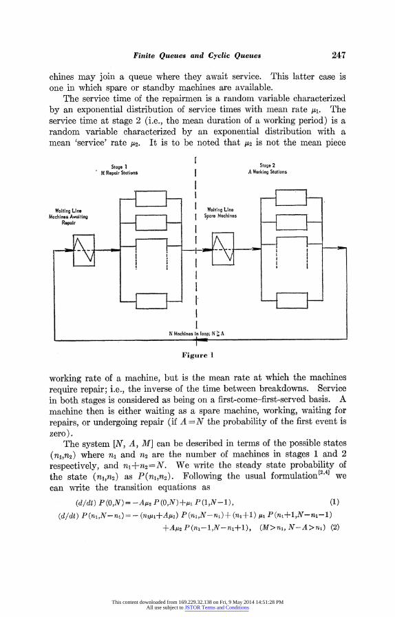
We consider the system shown in Fig. 1. There are N machines which move through the cycle. In stage 1, there are M repairmen; machines that have completed service at stage 1 (i.e., have been repaired) move on to stage 2, which is the working stage. The number of operators or works ing positions for the machines is A which is less than or equal to N. If A N the problem reduces to the Swedish machine problem, which has been extensively treated in the literature."""41 If A<N, repaired ma-
246
This content downloaded from 169.229.32.138 on Fri, 9 May 2014 14:51:28 PMAll use subject to JSTOR Terms and Conditions
Finite Queues and Cyclic Queues 247
chines may join a queue where they await service. This latter case is one in which spare or standby machines are available.
The service time of the repairmen is a random variable characterized by an exponential distribution of service times with mean rate Iu. The service time at stage 2 (i.e., the mean duration of a working period) is a random variable characterized by an exponential distribution with a mean 'service' rate 1X2. It is to be noted that /X2 is not the mean piece
Stage I Stage 2
M Repair Stations A Working Stations
Waiting Line Waiting Line Machines Awaiting Spare Machines
Repair
I 11 01 '] j~I
N Machines loop; N A
Figure 1
working rate of a machine, but is the mean rate at which the machines require repair; i.e., the inverse of the time between breakdowns. Service in both stages is considered as being on a first-come-first-served basis. A machine then is either waiting as a spare machine, working, waiting for repairs, or undergoing repair (if A= N the probability of the first event is zero) .
The system [N, A, M] can be described in terms of the possible states (nln2) where nl and n2 are the number of machines in stages 1 and 2 respectively, and nl+n2-N. We write the steady state probability of the state (nln2) as P(n1,n2). Following the usual formulation[24] we can write the transition equations as
(d/dt) P (O,N) =-A,2 P(0,N)?+p1 P(1,N-1), (1
(d/dt) P(niN-n;)= - (ncpc+AtiU2) P(n;,N-ni)+ (n-li) /t P(ni+1,N-n1-1)
+Apc P(nr-1,N-n1+1), (M>ni, N-A>nl) (2)
This content downloaded from 169.229.32.138 on Fri, 9 May 2014 14:51:28 PMAll use subject to JSTOR Terms and Conditions
248 Ernest Koenigsberg
(d/dt) P(ni,N-ni)= -(Mys+A.t2) P(ni,N-ni)+Mij P(nj+1,N-n1-1)
+AA2P(ni-1,N-ni+1), (M5ni<N-A) (3)
(d/dt) P(n ,N-nl)= -fnl ti+ (N-ni) ]21 P(n1,N-ni)
+ (ni+l),ui P(ni+1,N-nj-1)+ (N-n-+-) ,u2 P(ni-1,N-n+1?),
(M>ni>N-A) (4)
(d/dt) P (ni,N-n1 )=-[MI-t + (N-ni ) I'2j P(ni,N-nj)+Ml,/I P(nj+1,N-ni-1)
+ (N-nl+l) ,U2 P(ni-1,N-n,+1). (M1-<ni, N-A<ni) (5)
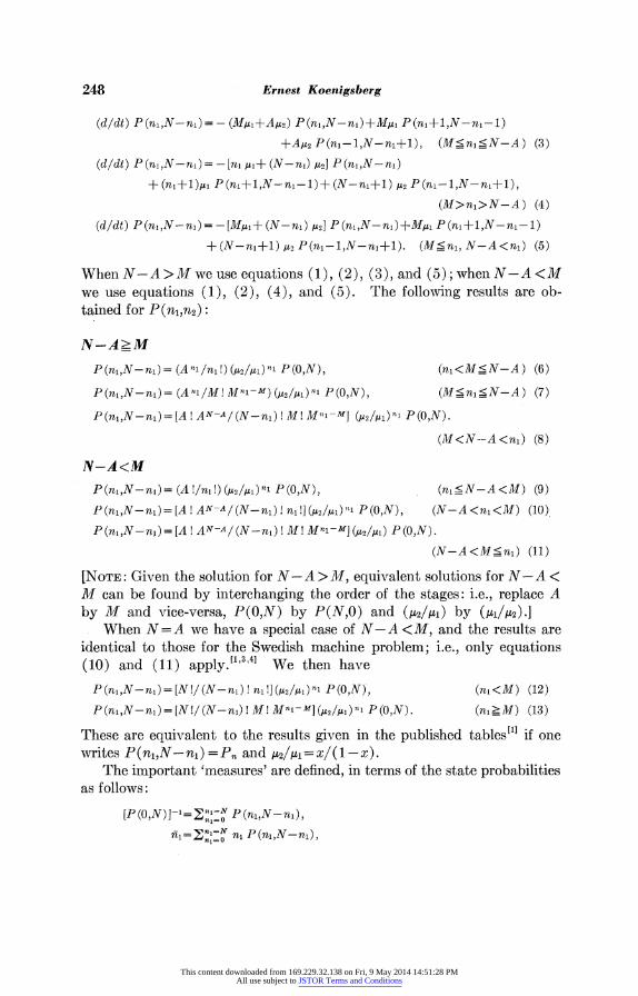
When N -A >M we use equations (1), (2), (3), and (5); when N -A <M we use equations (1), (2), (4), and (5). The following results are ob- tained for P(n1,n2):
N-AM
P(ni,N-ni)= (An,/n1!)(p2 /,-I) ni P(O,N), (ni<M<N-A) (6)
P(n,,N - ni)= (An, IM! Mt- M)("/1 n P (O,N), (M:!~nj: <N-A) (7)
? (n,,N- nj) = [A ! AN-A/ (N-ni) ! M:! M-1-m] (,u2/Pll) n' P (O,N).
(M<N--A<ni) (8)
N-A<M P(n,,N-nl)= (A !/nl !) (Y 2 /PI4lP (O,N), (nl <N-A<M) (9) P (ni,N- ni) = [A! AN-A/(N-nl)! ni !] (/2//1 ) P (0,N), (N-A <ni<M) (10),
P (nl ,N - nl) = [A ! AN-A / (N-n ) ! M !Mnl -M] (/u2//uL) P (O,N) .
(N-A<M5ni) (11)
[NOTE: Given the solution for N - A > M, equivalent solutions for N- A < M can be found by interchanging the order of the stages: i.e., replace A by M and vice-versa, P(O,N) by P(N,O) and ('2/41) by (1/,'2).]
When N - A we have a special case of N - A <M, and the results are identical to those for the Swedish machine problem; i.e., only equations (10) and (11) apply.""34' We then have
P (ni,N-ni ) = [N!/ (N-nl)! nli !] (Y2/,/1 ) n P (0,N), (ni<M) (12)
P (ni,N- ni) = [N!/ (N-ni)! M 1! Mnl-M] (&t2/b )nj P (0,N). (n1 _ M) (13)
These are equivalent to the results given in the published tables"1' if one writes P (ni,N-ni ) = Pn and g12/4=l -X/( I-x) .
The important 'measures' are defined, in terms of the state probabilities as follows:
[P (O0,N) ]-I = Pn,:N p (ni,N- ni.), nznl =N n, P (n,,N - n),
This content downloaded from 169.229.32.138 on Fri, 9 May 2014 14:51:28 PMAll use subject to JSTOR Terms and Conditions
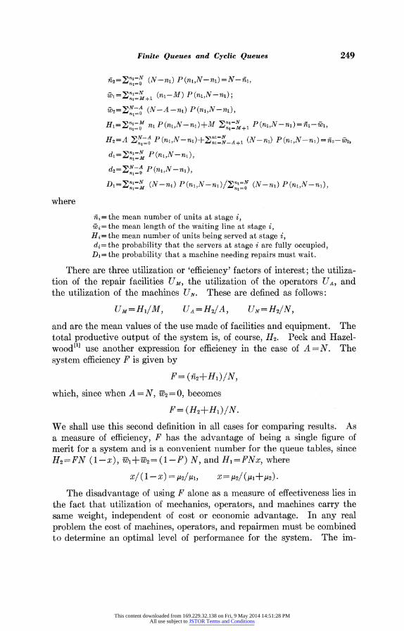
Finite Queues and Cyclic Queues 249
i2 =l-=N (N-n1) P(ni,N-ni)=N-fi1,
iW1 =:njN+ +1 (n - M) P (ni N - ni);
W2= ENjM (N-A-ni) P(ni,N-n1),
H1-= 'njM ni P (ni,N-ni) +M 2nl=N P(niN-nj)= ii-W,
H2=A n P(niN-A P) n-l N-A_-1 (N-ni) P(ni,N-nj)==i2-i2,
di = 2;nj N P (nlN-ni = A+
d2 =2N-A P(n,,N-ni),
D1i =2;njN (N-ni) P (nN-ni )/'nl=N (N-ni) P (n1,N-ni),
where
nii= the mean number of units at stage i, b =the mean length of the waiting line at stage i,
Hi= the mean number of units being served at stage i, di=the probability that the servers at stage i are fully occupied, D1= the probability that a machine needing repairs must wait.
There are three utilization or 'efficiency' factors of interest; the utiliza- tion of the repair facilities UM, the utilization of the operators UA, and the utilization of the machines UN. These are defined as follows:
UM = H1/M, UA= H2/A, UN=H2/N,
and are the mean values of the use made of facilities and equipment. The total productive output of the system is, of course, H2. Peck and Hazel- wood"1' use another expression for efficiency in the case of A N. The system efficiency F is given by
F= (fi2+H1)/N,
which, since when A =N, W2=0, becomes
F= (H2+fH1)/IN.
We shall use this second definition in all cases for comparing results. As a measure of efficiency, F has the advantage of being a single figure of merit for a system and is a convenient number for the queue tables, since H2=FN (1-X), w1+W2= (1-F) N, and Hi=FNx, where
X/I( 1 - X) )-Y21A, X - Y2/ (,41+,42) .
The disadvantage of using F alone as a measure of effectiveness lies in the fact that utilization of mechanics, operators, and machines carry the same weight, independent of cost or economic advantage. In any real problem the cost of machines, operators, and repairmen must be combined to determine an optimal level of performance for the system. The im-
This content downloaded from 169.229.32.138 on Fri, 9 May 2014 14:51:28 PMAll use subject to JSTOR Terms and Conditions
250 Ernest Koenigsberg
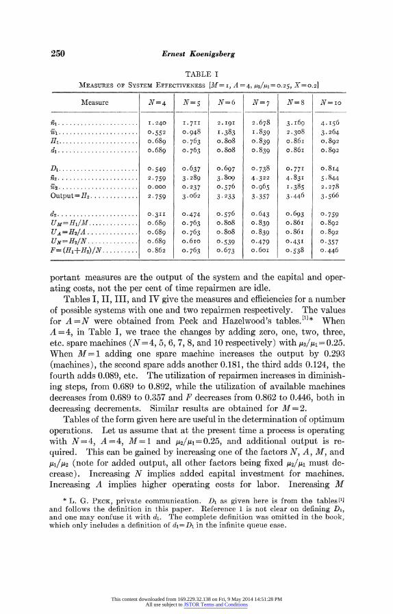
TABLE I
MEASURES OF SYSTEM EFFECTIVENESS [M-I, A 4, g2//l1= 0.25, X=0.21
Measure N=4 N=5 N=6 N=7 N=8 N= io
fl ..................... I. 240 I.71I 2. I9I 2.678 3. i69 4. I56 ...... .. ............ 0. 0552 0.948 I .383 I.839 2 .308 3.264 .....................0. o.689 0.763 o.8o8 o.839 o.86i 0.892
di ..................... 0. o.689 0.763 o .8o8 o.839 o.86i 0. 892
D1...................... 0- 549 o.637 o.697 0.738 0.77 o0.84
f12 ...................... 2.759 3. 289 3.809 4.322 4.831 5.844 W2 .0............... . .000 0.237 0.576 o0 965 1.385 2 . 278
Output= H2. . . . . . . . . . . . .2 759 3. o62 3. 233 3.357 3.446 3.566
d2 ......... ............0. o*3 0.474 0.576 o.643 o.693 0.759
UM= Hl/M0 *. . o0. 689 0.763 o .8o8 o.839 o.86i o0.892
UA =H2/A . . o 689 0.763 o .8o8 o.839 o.86I o0.892 UN1-H2/N . . o 689 o.6Io 0.539 0.479 0.431 0.357
F= (IH+H2)/N .......... o 862 0.763 o.673 o .6oi 0.538 0.446
portant measures are the output of the system and the capital and oper- ating costs, not the per cent of time repairmen are idle.
Tables 1, II, III, and IV give the measures and efficiencies for a number of possible systems with one and two repairmen respectively. The values for A=N were obtained from Peck and Hazelwood's tables" * When A 4, in Table I, we trace the changes by adding zero, one, two, three, etc. spare machines (N =4, 5, 6, 7, 8, and 10 respectively) with ,2/M1=0.25. When M=1 adding one spare machine increases the output by 0.293 (machines), the second spare adds another 0.181, the third adds 0.124, the fourth adds 0.089, etc. The utilization of repairmen increases in diminish- ing steps, from 0.689 to 0.892, while the utilization of available machines decreases from 0.689 to 0.357 and F decreases from 0.862 to 0.446, both in decreasing decrements. Similar results are obtained for M=2.
Tables of the form given here are useful in the determination of optimum operations. Let us assume that at the present time a process is operating with N = 4, A = 4, M =1 and 42/h1 == 0.25, and additional output is re- quired. This can be gained by increasing one of the factors N, A, M, and p11/2 (note for added output, all other factors being fixed /12/11 must de- crease). Increasing N implies added capital investment for machines. Increasing A implies higher operating costs for labor. Increasing M
* L. G. PECK, private communication. Di as given here is from the tabless[I] and follows the definition in this paper. Reference 1 is not clear on defining D1, and one may confuse it with di. The complete definition was omitted in the book, which only includes a definition of d1=D1 in the infinite queue case.
This content downloaded from 169.229.32.138 on Fri, 9 May 2014 14:51:28 PMAll use subject to JSTOR Terms and Conditions
Finite Queues and Cyclic Queues 251
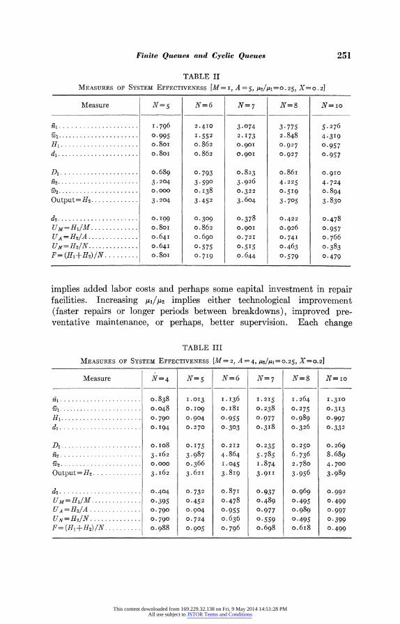
TABLE II
MEASURES OF SYSTEM EFFECTIVENESS [M=I, A =5, A11-2/1 =0.25, X 0.21
Measure N=5 N=6 N=7 N=8 N= io
* .. ................... I .796 2.4IO 3.074 3. 775 5. 276 , ,,,
............ ......... -0.995 I. 552 2. I73 2.848 4-3I9
H, .................. o.8oi o.862 0.90I 0.927 0.957
d. *.. . ...... o.8oi o0.862 0.90I 0.927 0.957
D1 .................. o.689 0.793 o.823 o.86i 0.9IO
F2................... 3.204 3 . 590 3.926 4.225 4- 724
W2 ...................o.0.000 0.I38 0.322 0-5I9 o.894
Output= H2 ............. 3.204 3.452 3.604 3.705 3.830
d2 .................... o 0.I99 0.309 0.378 0.422 0.478 UM = H1/M O . 8oi o0.862 0.90I 0.926 0 .957
UA = H2/A .............. o0.64I o0.690 0.72I 0. 74I 0 *766
UN = H21N .............. o. 64I 0 .575 0O5*5 0.463 O0.383 F= (H1+H2)/N. o.8oi 0. 7I9 O. 644 0.579 0.479
implies added labor costs and perhaps some capital investment in repair facilities. Increasing Ml/Y2 implies either technological improvement (faster repairs or longer periods between breakdowns), improved pre- ventative maintenance, or perhaps, better supervision. Each change
TABLE III
MEASURES OF SYSTEM EFFECTIVENESS [M= 2, A 4, /A2/1= 0. 25, X=0.2]
Measure N=4 N=5 N=6 N=7 N=8 N= io
l * *...................... , . 838 I.OI3 I.I36 I.2I5 I.264 I30IO
0.048 0. I09 o. i8i 0. 238 0. 275 0-3I3
H1 ....................0.790 0.904 0.955 0.977 o.989 0.997
di .................... 0. I94 0.270 0.303 0.3I8 0.326 0.332
D1 .................... O. io8 0.I75 0.2I2 0.235 0.250 0.269
2 *---.................... 3. I62 3.987 4.864 5.785 6.736 8.689 W2 ..........0............ o 000 0.366 I.045 I.874 2.780 4.700
Output=H2 ............. 3.I62 3.62I 3.8I9 3.9II 3.956 3.989
d2 ................... . o0.404 0.732 0.87I 0.937 o.969 0.992
UM = Hl/fM ...........0... 0395 0.452 0.478 0.489 0.495 0.499
UA= H21A ............0.. 0790 0.904 0.955 0.977 0.989 0.997 UN= H21N . ............. *790 0.724 o.636 0.559 0.495 0.399 F = (Hi+ H2) IN ............. o0.988 0.905 0.796 o.698 o.6i8 0.499
This content downloaded from 169.229.32.138 on Fri, 9 May 2014 14:51:28 PMAll use subject to JSTOR Terms and Conditions
252 Ernest Koenigsberg
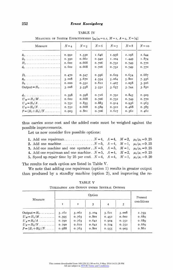
TABLE IV
MEASURES OF SYSTEM EFFECTIVENESS [2//4l1= 0.2, M= I, A 4, X = ']
Measure N=4 N=5 N=6 N=7 N=8 N= io
.................. .. o0.992 I * 330 I. 646 I .936 2. I98 2.644
..................... ?0.390 o0.662 0.940 I. 204 I .449 I. 874 H.0....... o.602 o.668 0.706 0.732 0.749 0.770
d. o.602 o.668 0 .706 0.732 0.749 0.770
Di .................... 0.470 0.547 0.596 o.629 o.654 o.687 2. .3.008 3.670 4.354 5. o64 5.802 7.356 2. .. .................... 0.000 0.332 0.822 I .407 2.058 3.506
Output = 112 . . . . .... ..... 3. oo8 3 . 338 3.532 3.657 3.744 3.850
d2 .0.................... 0.398 0.598 0.7i6 0.792 o0 845 0. 909 UM=H1/M .. 602 o.668 0.706 0.732 0.749 0.770 UA=H2/A .0.752 o.835 o0.883 0.914 0.936 o 963 UN= H2/N .....0.. 0-752 o.668 0.589 0.522 0.468 0.385 F= (HI+H2)/IN ......... -0.903 o.8oi 0 .706 o.627 0.562 0.462
thus carries some cost and the added costs must be weighed against the possible improvements.
Let us now consider five possible options:
1. Add one repairman ............... N =4, A =4, M=2, Y2/g1= O. 25 2. Add one machine ............... N =5, A =4, 1M1, = 2/gi = O. 25 3. Add one machine and one operator. .N=5, A =5, 1M =1, A2/Y11=0.25 4. Add one repairman and one machine. AN = 5, A =4, lI = 2, u2/Al = 0.25 5. Speed up repair time by 25 per cent. . N =4, A =4, I-=i, bt2/Al =0.20
The results for each option are listed in Table V. We note that adding one repairman (option 1) results in greater output
than produced by a standby machine (option 2), and improving the re-
TABLE V
UTILIZATION AND OUTPUT UNDER SEVERAL OPTIONS
Measure - ________ - Option Present
Measure conditions I 2 3 4 5
Output = H2 ......... 3. I62 3. o62 3.204 3.621 3. oo8 2.759 UM=H .../M..0.395 0.763 o.8oi 0.452 o.602 o.689 UA = H2/A .......... 0790 0.763 o.64I 0.904 0.752 O 689 UN = H2/N . 0.790 o.6io O. 64I 0.724 0.752 o.689 F= (H1--H2)/N ..... o0.988 0.763 o.8oi 0.955 0.903 o.862
This content downloaded from 169.229.32.138 on Fri, 9 May 2014 14:51:28 PMAll use subject to JSTOR Terms and Conditions
Finite Queues and Cyclic Queues 253
pair facility (option 5) is almost as fruitful as purchasing a standby ma- chine In many cases repair facilities are cheaper than an added produc- tion unit; if this is so, and the added output is sufficient, option 1 may be preferred. We also note that adding a machine and a repairman (option 4) produces greater output than adding a machine and an operator (option 3). This again shows that repair facilities should not be overlooked in any plan for increased production.
Thus, it is clear that consideration of the cyclic process leads to the logical extension of finite queue processes such as the Swedish machine problem. The spare or standby machine problem is one example that can be treated by this method. The cyclic process is also applicable to problems in which repair and/or operation of machines requires more than one stage. As an example of a 3-stage process one would have an inspection and/or tuneup stage between the repair and productive opera- tionS Alternatively there is the case of reparable spare parts for a fleet of aircraft or trucks. In such cases one frequently finds a transportation and inventory process between the repair facility and the items in opera- tion. Some work along these lines has already been earned outs
REFERENCES
L. L. G. PECK AND R. N. HAZELWOOD, Finite Queauin Tables, ORSA Publica- tions in Operations Research, No. 2, Wiley, New York, 1958.
2. E. KOENIGSBERG, Operational Research Quarterly 9, 22-35 (1958) 3. C. PALm, Industritidningen Norden 75, 75-80, 90-94, 119-123 (1957). 4t W. FELLER, Introductito to Probability Theory and Jts Application, Wiley, New
York, 1940.
This content downloaded from 169.229.32.138 on Fri, 9 May 2014 14:51:28 PMAll use subject to JSTOR Terms and Conditions