FINITE GENERATION OF SOME COHOMOLOGY …sjw/pub/cohp3journal2017115.pdf · Note that the zero term of grH equals its coradical, i.e., (grH) 0 = H 0. There is a projection ˇ: grH!H

FINITE GENERATION OF SOME COHOMOLOGY RINGS

VIA TWISTED TENSOR PRODUCT AND ANICK RESOLUTIONS

VAN C. NGUYEN, XINGTING WANG, AND SARAH WITHERSPOON

Abstract. Over a field of prime characteristic p > 2, we prove that the cohomology rings of somepointed Hopf algebras of dimension p3 are finitely generated. These are Hopf algebras arising inthe ongoing classification of finite dimensional Hopf algebras in positive characteristic, and includebosonizations of Nichols algebras of Jordan type in a general setting as well as their liftings whenp = 3. Our techniques are applications of twisted tensor product resolutions and Anick resolutionsin combination with May spectral sequences.

Contents

1. Introduction 12. Settings 22.1. Pointed Hopf algebras 22.2. Our setting: Rank two Nichols algebra and its bosonization 32.3. Our setting: A class of 27-dimensional pointed Hopf algebras 33. Twisted tensor product resolutions 43.1. The resolution construction 43.2. Resolution over the Nichols algebra R 53.3. Resolution over the bosonization R#kG 84. Anick resolutions 114.1. The resolution construction 114.2. A truncated polynomial ring 155. Finite generation of some cohomology rings 175.1. Cohomology of the Nichols algebra and its bosonization 175.2. Cohomology of some pointed Hopf algebras of dimension 27 19References 20

1. Introduction

The cohomology ring of a finite dimensional Hopf algebra is conjectured to be finitely generated.Friedlander and Suslin [8] proved this for cocommutative Hopf algebras, generalizing earlier resultsof Evens [6], Golod [10], and Venkov [24] for finite group algebras and of Friedlander and Parshall [7]for restricted Lie algebras. There are many finite generation results as well for various typesof noncocommutative Hopf algebras (see, e.g., [3, 9, 11, 14, 22]). Most of these results are incharacteristic 0. In this paper, we prove finite generation for classes of noncocommutative Hopf

Date: November 5, 2017.2010 Mathematics Subject Classification. 16E05, 16E40, 16T05.Key words and phrases. cohomology, positive characteristic, (pointed) Hopf algebras, Anick resolutions, twisted

tensor products.The third author was partially supported by NSF grant DMS-1401016.

1

2 VAN C. NGUYEN, XINGTING WANG, AND SARAH WITHERSPOON

algebras in prime characteristic p > 2. These are some of the pointed Hopf algebras arising inclassification work of the first two authors.

Our main result is the following combination of Theorems 5.1.2 and 5.2.1 below:

Theorem. Let k be an algebraically closed field of prime characteristic p > 2. Consider thefollowing Hopf algebras over k:

(1) the p2q-dimensional bosonization R#kG of a rank two Nichols algebra R of Jordan typeover a cyclic group G of order q, where q is divisible by p; and

(2) a lifting H of R#kG when p = q = 3.

Then the cohomology rings of R#kG and of H are finitely generated.

Our theorem is exclusively an odd characteristic result since the Nichols algebra of Jordan typedoes not appear in characteristic 2. Instead there is another related Nichols algebra [4] that willrequire different techniques. Part (2) of our main theorem above is only stated for characteristic 3;this is because we use the classification of such Hopf algebras from [18], and liftings are only knowncompletely in this case. We expect our homological techniques will be able to handle liftings whenp > 3 once more is known about their structure.

More specifically, we let R#kG be a p2q-dimensional Hopf algebra given by the bosonization ofa Jordan plane as introduced in [4] (see Section 2.2 below). We prove in Theorem 5.1.2 that thecohomology ring of such a Hopf algebra R#kG, that is H∗(R#kG,k) := Ext∗R#kG(k,k), is finitely

generated. We also consider liftings H of R#kG in the special case p = q = 3 (see Section 2.3below). We prove in Theorem 5.2.1 that the cohomology ring H∗(H,k) is finitely generated.

Our techniques for proving the main theorem above rely on the May spectral sequence for thecohomology of a filtered algebra. In either setting, (1) or (2), we may choose a filtration for whichthe associated graded algebra is a truncated polynomial ring whose cohomology is straightforward.The hard work is in finding some permanent cycles as required to use a spectral sequence lemmathat goes back to Friedlander and Suslin [8]. This we do in two ways, by constructing two types ofresolutions which should be of independent interest. The general definitions of the resolutions arenot new, but we provide here some nontrivial examples, with our main theorem as an application.The first resolution is the twisted tensor product resolution of [20], recalled in Section 3.1, used inSection 3.2, and iterated in Section 3.3, to obtain a resolution over the bosonization R#kG of theNichols algebra R. This is used in Section 5.1 to prove finite generation of its cohomology. Thesecond resolution is the Anick resolution [1], explained in Section 4.1, with a general result for theAnick resolution of a truncated polynomial ring in Section 4.2. This Anick resolution is used inSection 5.2 to prove finite generation of the cohomology of the liftings H. We could have chosento work with just one type of resolution construction, either Anick or twisted tensor product, forproofs of both parts (1) and (2) of our main theorem above. We instead chose to work with bothto illustrate a wider variety of techniques available, each having its own advantages.

2. Settings

Throughout, let k be a field. For our main results we will assume that k is algebraically closedof prime characteristic p > 2 since we work with Hopf algebras found in classification work underthis assumption. The tensor product ⊗ is ⊗k and 1 denotes the identity map on any set unlessspecified otherwise. In this section, we will define the Nichols algebras and pointed Hopf algebrasthat are featured in this paper, and summarize some structural results that will be needed.

2.1. Pointed Hopf algebras. Let H be any finite dimensional pointed Hopf algebra over k. Thecoradical (the sum of all simple subcoalgebras) of H is H0 = kG, a Hopf subalgebra of H generatedby the grouplike elements G := {g ∈ H |∆(g) = g ⊗ g}, where ∆ is the coproduct on H.

LetH0 ⊆ H1 ⊆ H2 ⊆ · · · ⊆ H

COHOMOLOGY OF POINTED HOPF ALGEBRAS 3

be the coradical filtration of H, where Hn = ∆−1(H⊗Hn−1+H0⊗H) inductively, see [17, Chapter5]. Consider the associated graded Hopf algebra grH =

⊕n≥0Hn/Hn−1, with the convention

H−1 = 0. Note that the zero term of grH equals its coradical, i.e., (grH)0 = H0. There is aprojection π : grH → H0 and an inclusion ι : H0 → grH such that πι = 1H0 . Let R be the algebraof coinvariants of π:

R := (grH)co π = {h ∈ grH : (1H ⊗ π)∆(h) = h⊗ 1}.

By results of Radford [23] and Majid [15], R is a Hopf algebra in the braided category GGYD of left

Yetter-Drinfeld modules over H0 = kG. Moreover, grH is the bosonization (or Radford biproduct)of R and H0 so that grH ∼= R#H0 with the Hopf structure given in [17, Theorem 10.6.5]. As analgebra, it is simply the smash product of H0 with R, analogous to a semidirect product of groups.

2.2. Our setting: Rank two Nichols algebra and its bosonization. For Sections 3 and 5.1,we use the following setup. Let k be a field of prime characteristic p > 2. Let G := 〈g〉 ∼= Z/qZ bea cyclic group whose order q is divisible by p. Consider

R := k〈x, y〉/(

xp, yp, yx− xy − 1

2x2),

which is a p2-dimensional algebra as described in [4, Theorem 3.5], with a vector space basis{xiyj | 0 ≤ i, j ≤ p − 1}. Observe that R is the Nichols algebra of a rank two Yetter-Drinfeldmodule V = kx+ ky over G, where the G-action on V is given by

gx = x and gy = x+ y

(here, left superscript indicates group action), and the G-gradings of x and y are both given by g.Let R#kG be the bosonization of R and kG. It is the corresponding p2q-dimensional pointed

Hopf algebra as studied in [4, Corollary 3.14], [18, §3 (Case B)], and [19, §4]. Its Hopf structure isgiven by:

∆(x) = x⊗ 1 + g ⊗ x, ∆(y) = y ⊗ 1 + g ⊗ y, ∆(g) = g ⊗ g,ε(x) = 0, ε(y) = 0, ε(g) = 1,

S(x) = −g−1x, S(y) = −g−1y, S(g) = g−1,

where ∆ is the coproduct, ε is the counit, and S is the antipode map of R#kG.

Remark 2.2.1. These algebras have featured in the following papers:

(1) These R,G,R#kG appear in [4, 18, 19] for various purposes. In their settings, G is a cyclicgroup of order p. Here, we consider a more general setting with G being cyclic of order qdivisible by p.

(2) In [18], the first two authors classified p3-dimensional pointed Hopf algebra over primecharacteristic p. In their classification work, this p2-dimensional Nichols algebra R of Jordantype is unique, up to isomorphism, and only occurs when p > 2.

(3) The authors of [4] used right modules in their settings, whereas left modules were used in[18], thus inducing a sign difference in the relation yx−xy− 1

2x2 of R there. Here, we adopt

the relation described in [4]. In Section 5.2, when we study the cohomology of pointedHopf algebras H lifted from the associated graded algebras grH ∼= R#kG, we modify therelations of the lifting structure given in [18] accordingly, see the next Section 2.3.

2.3. Our setting: A class of 27-dimensional pointed Hopf algebras. Let k be a field ofcharacteristic p = 3 and consider Hopf algebras H(ε, µ, τ) defined from three scalar parametersε, µ, τ as in [18]. These are pointed Hopf algebras of dimension 27 whose associated graded algebrais grH(ε, µ, τ) ∼= R#kG, the Hopf algebra described in Section 2.2, in this case p = q = 3.


As an algebra, H(ε, µ, τ) is generated by g, x, y with relations

g3 = 1, x3 = εx, y3 = −εy2 − (µε− τ − µ2)y,yg − gy = xg + µ(g − g2), xg − gx = −ε(g − g2),

yx− xy = −x2 + (µ+ ε)x+ εy + τ(1− g2),

where ε ∈ {0, 1} and τ, µ ∈ k are arbitrary scalars. The coalgebra structure is the same as thatof R#kG described in Section 2.2. By setting w = g − 1, we get a new presentation in which thegenerators are w, x, y and the relations are:

w3 = 0, x3 = εx, y3 = −εy2 − (µε− τ − µ2)y,yw − wy = wx+ x− (µ− ε)(w2 + w), xw − wx = ε(w2 + w),

yx− xy = −x2 + (µ+ ε)x+ εy − τ(w2 − w).

This choice of generating set will be convenient for our homological arguments later. As shownin [18], H(ε, µ, τ) has dimension 27. It has vector space basis {wixjyk | 0 ≤ i, j, k ≤ 2}.

3. Twisted tensor product resolutions

In this section, we apply the construction of twisted tensor product resolutions introduced in[20] to our Nichols algebra R and its bosonization R#kG that was defined in Section 2.2.

3.1. The resolution construction. Let A and B be associative algebras over k with multiplica-tion maps mA : A⊗A→ A, mB : B ⊗B → B, and multiplicative identities 1A, 1B, respectively.

A twisting map τ : B⊗A→ A⊗B is a bijective k-linear map for which τ(1B ⊗ a) = a⊗ 1B andτ(b⊗ 1A) = 1A ⊗ b, for all a ∈ A and b ∈ B, and

(3.1.1) τ ◦ (mB ⊗mA) = (mA ⊗mB) ◦ (1⊗ τ ⊗ 1) ◦ (τ ⊗ τ) ◦ (1⊗ τ ⊗ 1)

as maps B⊗B⊗A⊗A→ A⊗B. The twisted tensor product algebra A⊗τB is the vector space A⊗Btogether with multiplication mτ given by such a twisting map τ , that is, mτ : (A⊗B)⊗ (A⊗B)→A⊗B is given by mτ = (mA ⊗mB) ◦ (1⊗ τ ⊗ 1).

Definition 3.1.2. [20, Definition 5.1] Let M be an A-module with module structure map ρA,M :A⊗M →M . We say M is compatible with the twisting map τ if there is a bijective k-linear mapτB,M : B ⊗M →M ⊗B such that

τB,M ◦ (mB ⊗ 1) = (1⊗mB) ◦ (τB,M ⊗ 1) ◦ (1⊗ τB,M ), and(3.1.3)

τB,M ◦ (1⊗ ρA,M ) = (ρA,M ⊗ 1) ◦ (1⊗ τB,M ) ◦ (τ ⊗ 1)(3.1.4)

as maps on B ⊗B ⊗M and on B ⊗A⊗M , respectively.

Let M be an A-module that is compatible with τ . We say a projective A-module resolution P q(M)of M is compatible with the twisting map τ if each module Pi(M) is compatible with τ via maps τB,ifor which τB, q : B⊗P q(M)→ P q(M)⊗B is a k-linear chain map lifting τB,M : B⊗M →M⊗B. LetN be a B-module and let P q(N) be a projective resolution of N over B. We put an A⊗τ B-modulestructure on the bicomplex P q(M)⊗ P q(N) by using maps τB, q.

Under such compatibility conditions, the twisted tensor product resolutions for left modules overA⊗τ B were constructed in [20] satisfying the following theorem.

Theorem 3.1.5. [20, Theorem 5.12] Let A and B be k-algebras with twisting map τ : B ⊗ A →A⊗B. Let P q(M) be an A-projective resolution of M and P q(N) be a B-projective resolution of N .Assume

(a) M and P q(M) are compatible with τ , and(b) Yi,j = Pi(M)⊗ Pj(N) is a projective A⊗τ B-module, for all i, j.


Then the twisted tensor product complex Y q = Tot(P q(M)⊗ P q(N)) with

Yn =⊕i+j=n

Pi(M)⊗ Pj(N)

is a projective resolution of M ⊗N as a module over the twisted tensor product A⊗τ B.

By Tot(P q(M)⊗P q(N)) we mean the total complex of the bicomplex P q(M)⊗P q(N), that is thecomplex whose nth component is Yn = ⊕i+j=n(Pi(M)⊗Pj(N)) and differential is dn =

∑i+j=n dij

where dij = di ⊗ 1 + (−1)i1⊗ dj .In the statement of [20, Theorem 5.12], we have replaced one of the hypotheses by our hypoth-

esis (b) above, and in this case the proof is given by [20, Lemmas 5.8 and 5.9]. In some contexts,such as ours here, the hypothesis (b) can be checked directly, in which case this version of thetheorem is sufficient.

For the rest of this section, let k be a field of characteristic p > 2 and R,G be as described inSection 2.2. Let k also denote the trivial (left) R- or (R#kG)-module, that is, the field k withaction given by the augmentation ε(x) = 0, ε(y) = 0, ε(g) = 1. We will construct a resolution of kas an R-module via a twisted tensor product, and as an (R#kG)-module by iterating the twistedproduct construction.

3.2. Resolution over the Nichols algebra R. We start with a construction of a resolution of kover R. Using the relation (3.9) in [4, Lemma 3.8], we can view R as the twisted tensor product

R = k〈x, y〉/(

xp, yp, yx− xy − 1

2x2)∼= A⊗τ B,

where A := k[x]/(xp), B := k[y]/(yp). The twisting map τ : B ⊗A→ A⊗B is defined by

τ(yr ⊗ x`) =r∑t=0

(r

t

)(1

2

)t[`][t] x`+t ⊗ yr−t,

where we use the convention:

[`][t] = `(`+ 1)(`+ 2) · · · (`+ t− 1),

with [`][0] = 1, for any `.Consider the following free resolutions of k as A-module and as B-module, respectively:

P q(A) : · · · xp−1· // A

x· // Axp−1· // A

x· // Aε // k // 0

P q(B) : · · ·yp−1· // B

y· // Byp−1· // B

y· // Bε // k // 0.

The map ε on A (respectively, on B) takes x to 0 (respectively, y to 0). Consider the tensorproduct P q(A)⊗ P q(B) as a graded vector space. The total complex is a complex of vector spaceswith differential in degree n given by

dn =∑i+j=n

di ⊗ 1 + (−1)i1⊗ dj .

We will put the structure of an R-module on each Pi(A)⊗Pj(B) so that this tensor product complexis an R-projective resolution of k as an R-module. This will follow from [20, Lemmas 5.8 and 5.9]once we define a chain map as in Definition 3.1.2 and check that the resulting R-modules are indeed


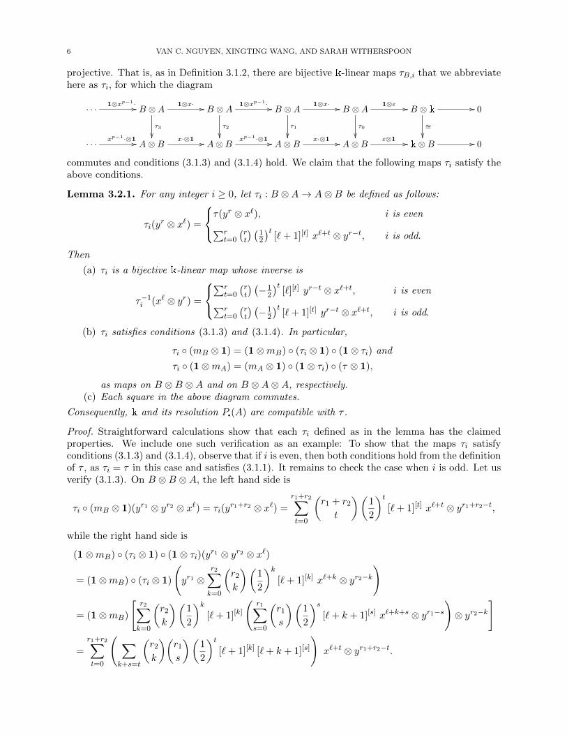
projective. That is, as in Definition 3.1.2, there are bijective k-linear maps τB,i that we abbreviatehere as τi, for which the diagram

· · · 1⊗xp−1· // B ⊗A

τ3

��

1⊗x· // B ⊗A

τ2

��

1⊗xp−1· // B ⊗A

τ1

��

1⊗x· // B ⊗A

τ0

��

1⊗ε // B ⊗ k //

∼=��

0

· · · xp−1·⊗1 // A⊗B x·⊗1 // A⊗B xp−1·⊗1 // A⊗B x·⊗1 // A⊗B ε⊗1 // k⊗B // 0

commutes and conditions (3.1.3) and (3.1.4) hold. We claim that the following maps τi satisfy theabove conditions.

Lemma 3.2.1. For any integer i ≥ 0, let τi : B ⊗A→ A⊗B be defined as follows:

τi(yr ⊗ x`) =

τ(yr ⊗ x`), i is even∑rt=0

(rt

) (12

)t[`+ 1][t] x`+t ⊗ yr−t, i is odd.

Then

(a) τi is a bijective k-linear map whose inverse is

τ−1i (x` ⊗ yr) =

∑r

t=0

(rt

) (−1

2

)t[`][t] yr−t ⊗ x`+t, i is even∑r

t=0

(rt

) (−1

2

)t[`+ 1][t] yr−t ⊗ x`+t, i is odd.

(b) τi satisfies conditions (3.1.3) and (3.1.4). In particular,

τi ◦ (mB ⊗ 1) = (1⊗mB) ◦ (τi ⊗ 1) ◦ (1⊗ τi) and

τi ◦ (1⊗mA) = (mA ⊗ 1) ◦ (1⊗ τi) ◦ (τ ⊗ 1),

as maps on B ⊗B ⊗A and on B ⊗A⊗A, respectively.(c) Each square in the above diagram commutes.

Consequently, k and its resolution P q(A) are compatible with τ .

Proof. Straightforward calculations show that each τi defined as in the lemma has the claimedproperties. We include one such verification as an example: To show that the maps τi satisfyconditions (3.1.3) and (3.1.4), observe that if i is even, then both conditions hold from the definitionof τ , as τi = τ in this case and satisfies (3.1.1). It remains to check the case when i is odd. Let usverify (3.1.3). On B ⊗B ⊗A, the left hand side is

τi ◦ (mB ⊗ 1)(yr1 ⊗ yr2 ⊗ x`) = τi(yr1+r2 ⊗ x`) =

r1+r2∑t=0

(r1 + r2

t

)(1

2

)t[`+ 1][t] x`+t ⊗ yr1+r2−t,

while the right hand side is

(1⊗mB) ◦ (τi ⊗ 1) ◦ (1⊗ τi)(yr1 ⊗ yr2 ⊗ x`)

= (1⊗mB) ◦ (τi ⊗ 1)

(yr1 ⊗

r2∑k=0

(r2k

)(1

2

)k[`+ 1][k] x`+k ⊗ yr2−k

)

= (1⊗mB)

[r2∑k=0

(r2k

)(1

2

)k[`+ 1][k]

(r1∑s=0

(r1s

)(1

2

)s[`+ k + 1][s] x`+k+s ⊗ yr1−s

)⊗ yr2−k

]

=

r1+r2∑t=0

( ∑k+s=t

(r2k

)(r1s

)(1

2

)t[`+ 1][k] [`+ k + 1][s]

)x`+t ⊗ yr1+r2−t.


It is straightforward to check that [`+ 1][k] [`+ k + 1][s] = [`+ 1][k+s], and

t∑k=0

(r2k

)(r1t− k

)=

(r1 + r2

t

).

This gives us the equality (3.1.3) as desired. �

For each i, the map τi is used to give Pi(A)⊗ Pj(B) = A⊗ B the structure of a left (A⊗τ B)-module. In the case when i is even, this is the usual (A⊗τ B)-module structure. In the case wheni is odd, the (A⊗τ B)-module structure via τi is given by

(A⊗τ B)⊗ (A⊗B)1⊗τi⊗1 // A⊗A⊗B ⊗B mA⊗mB // A⊗B.

Lemma 3.2.2. Retaining the above module structure, Pi(A)⊗ Pj(B) = A⊗B is a free (A⊗τ B)-module of rank one, generated by 1⊗ 1, via the (A⊗τ B)-module isomorphism ϕ : A⊗τ B → A⊗Bgiven by

ϕ(x` ⊗ yr) =

{x` ⊗ yr, i is even∑r

t=0

(rt

)t!2t x

`+t ⊗ yr−t, i is odd,

whose inverse is given by

ϕ−1(x` ⊗ yr) =

{x` ⊗ yr, i is even

x` ⊗ yr − r2x

`+1 ⊗ yr−1, i is odd.

Proof. When i is even, ϕ is clearly bijective. We check that ϕ is a bijection with the given inversewhen i is odd:

ϕ ◦ ϕ−1(x` ⊗ yr) = ϕ(x` ⊗ yr − r

2x`+1 ⊗ yr−1

)=

r∑t=0

(r

t

)t!

2tx`+t ⊗ yr−t − r

2

r−1∑k=0

(r − 1

k

)k!

2kx`+1+k ⊗ yr−1−k

= x` ⊗ yr +r∑t=1

(r

t

)t!

2tx`+t ⊗ yr−t −

r∑t=1

r

(r − 1

t− 1

)(t− 1)!

2tx`+t ⊗ yr−t

= x` ⊗ yr +r∑t=1

((r

t

)t− r

(r − 1

t− 1

))(t− 1)!

2tx`+t ⊗ yr−t

= x` ⊗ yr +

r∑t=1

(0)(t− 1)!

2tx`+t ⊗ yr−t = x` ⊗ yr.

By (3.1.4), ϕ is a module isomorphism. Therefore A⊗B is free as an (A⊗τ B)-module. �

In particular, the following is useful for our computations later:

ϕ−1(1⊗ y) =

{1⊗ y, i is even

1⊗ y − 12x⊗ 1, i is odd,

ϕ−1(1⊗ yp−1) =

{1⊗ yp−1, i is even

1⊗ yp−1 + 12x⊗ y

p−2, i is odd.

(3.2.3)

By Theorem 3.1.5, the total complex K q := Tot(P q(A) ⊗ P q(B)) is a free resolution of k asA ⊗τ B-module. For each i, j ≥ 0, let φi,j denote the free generator 1 ⊗ 1 of Pi(A) ⊗ Pj(B) as anA⊗τ B-module. Then as an R-module:

Kn =⊕i+j=n

Rφi,j .


Recall that the differentials of this total complex are dn =∑

i+j=n(di ⊗ 1 + (−1)i1 ⊗ dj). As

Pi(A)⊗Pj(B) is free as an A⊗τ B-module with generator φi,j , we can write the image of φi,j underthe differential map as the action of A⊗τ B on φi,j , using values of the inverse map ϕ−1 defined in(3.2.3) where needed. We express the differential on elements via this notation:

d(φi,j) =

xp−1φi−1,j + yp−1φi,j−1 if i, j are even,

xp−1φi−1,j + yφi,j−1 if i is even and j is odd,

xφi−1,j − (yp−1 + 12xy

p−2)φi,j−1 if i is odd and j is even,

xφi−1,j − (y − 12x)φi,j−1 if i, j are odd.

We interpret φi,j to be 0 if either i or j is negative.

3.3. Resolution over the bosonization R#kG. Again we take k to be a field of characteristicp > 2 and R, G as described in Section 2.2. For the group G = 〈g〉 ∼= Z/qZ, where q is divisibleby p, we define an action of G on the R-complex K q constructed in Section 3.2, for the purpose offorming a twisted tensor product resolution of K q with a resolution of k as kG-module. The groupaction will give us a twisting map on the complex K q analogous to the twisting map defining a skewgroup algebra. The resulting complex will give us a resolution of k over the bosonization R#kG.

Let R = A ⊗τ B be the twisted tensor product with A := k[x]/(xp), B := k[y]/(yp) andτ : B ⊗ A → A ⊗ B as defined before. Under our setting in characteristic p > 2 and relationyx = xy + 1

2x2 in R, we obtain the following relations in R by straightforward calculations (here,

we drop the tensor symbols and write xy in place of x⊗ y in R):

• For any integer ` ≥ 0, yx` = x`y +`

2x`+1.

• For any integer n ≥ 1, (x+ y)n =n∑i=0

(n

i

)(i+ 1)!

2ixiyn−i.

Further calculations show the following.

Lemma 3.3.1. Define an element

α := −yp−2 +

p−2∑i=1

(−1)i+1 (i+ 1)!

2i+1xiyp−2−i ∈ R.

Then α satisfies the following:

(a) xα = (x+ y)p−1 − yp−1 + 12x[(x+ y)p−2 − yp−2] ,

(b) (x+ y)α = −yp−1 − 12xy

p−2 ,

(c) αx = (x+ y)p−1 − yp−1 ,

(d) α(y − 12x) = −(x+ y)p−1.

Recall that G = 〈g〉 ∼= Z/qZ acts on R by gx = x and gy = x+ y. We define an action of G onthe complex K q, constructed in Section 3.2, as follows: for all 0 ≤ s ≤ q − 1,

gsφi,j =

φi,j , if i is oddφi,j + s φi+1,j−1, if i is even and j is odd

φi,j + ((gs−1+···+g+1)α)φi+1,j−1, if i, j are even.

Moreover, it is not hard to figure out the following for all 1 ≤ s ≤ q,

g−sφi,j =

φi,j , if i is oddφi,j − s φi+1,j−1, if i is even and j is odd

φi,j − ((g−s+···+g−1)α)φi+1,j−1, if i, j are even.

(3.3.2)


Lemma 3.3.3. With the above G-action, the complex K q is G-equivariant.

Proof. We first show that this G-action is well-defined, that is, gqφi,j = φi,j .

It is clear that when i is odd, or when i is even and j is odd that gqφi,j = φi,j , as q is divisibleby the characteristic p of the field k. When i, j are both even, we need to show that

gqφi,j = φi,j + ((gq−1+···+g+1)α)φi+1,j−1 = φi,j ,

that is, we need to show (gq−1+···+g+1)α = 0.From Lemma 3.3.1 (c), we have αx = (x+ y)p−1 − yp−1. Now apply gs to both sides to obtain:

gsα gsx = (gsx+ gsy)p−1 − (g

sy)p−1,

gsα x = (x+ y + sx)p−1 − (y + sx)p−1.

Thus, summing over all 0 ≤ s ≤ q − 1:(q−1∑s=0

gsα

)x =

q−1∑s=0

([y + (s+ 1)x]p−1 − (y + sx)p−1

)= (y + qx)p−1 − yp−1 = 0.

So∑q−1

s=0gsα = 0 in the domain k〈x, y〉/(yx− xy − 1

2x2) and hence is also 0 in R. Therefore, in all

cases, we have gqφi,j = φi,j and the above G-action is well-defined.To check that the complex K q is G-equivariant, we need to check such G-action is compatible

with the differential maps in each degree, that is, d( gφi,j) = gd(φi,j), for all i, j ≥ 0. When i andj are both even:

d( gφi,j) = d(φi,j + αφi+1,j−1)

= xp−1φi−1,j + yp−1φi,j−1 + α

(xφi,j−1 − (y − 1

2x)φi+1,j−2

),

gd(φi,j) = gxp−1 gφi−1,j + gyp−1 gφi,j−1

= xp−1φi−1,j + (x+ y)p−1(φi,j−1 + φi+1,j−2).

Comparing, we see that coefficients for the terms φi,j−1 and φi+1,j−2 are exactly identities (c) and(d) in Lemma 3.3.1, respectively. The other cases are similar by applying Lemma 3.3.1, and wehave d( gφi,j) = gd(φi,j) for all i, j, g. Thus, the complex K q is G-equivariant. �

We use this G-action next to form a twisted tensor product resolution of k as an R#kG-module.Let the twisting map τ ′n : kG⊗Kn → Kn ⊗ kG be given by the action of G on Kn, so that

τ ′i+j(g ⊗ φi,j) =

φi,j ⊗ g, if i is odd(φi,j + φi+1,j−1)⊗ g, if i is even and j is odd(φi,j + αφi+1,j−1)⊗ g, if i, j are even.

Then K q is compatible with τ ′ (giving the twisting that governs the smash product construction)via the maps τ ′n.

Let P q(kG) be the following free resolution of the trivial kG-module k:

P q(kG) : · · ·(∑q−1

s=0 gs)·// kG

(g−1)· // kG(∑q−1

s=0 gs)·// kG

(g−1)· // kGε // k // 0,

where ε takes g to 1.Let Y q := Tot(K q ⊗ P q(kG)). The modules are free (R#kG)-modules by a similar argument to

what we used earlier: In each degree we have a direct sum of modules of the form R ⊗ kG. Eachsuch is freely generated by some φi,j ⊗ φk, where φk denotes the free generator for Pk(kG) = kG.So by Theorem 3.1.5, Y q is a free resolution of the (R#kG)-module k.


For each i, j, k ≥ 0, let φi,j,k denote the free generator φi,j⊗φk of Ki+j⊗Pk(kG) as an (R#kG)-module. We set φi,j,k = 0 if one of i, j, k is negative. Then, for all n ≥ 0, as an (R#kG)-module,

Yn =⊕

i+j+k=n

(R#kG)φi,j,k.

We express the differentials on elements as follows, where d(φi,j) is given at the end of Section 3.2:

d(φi,j,k) = d(φi,j)⊗ φk

+ (−1)i+j

(g − 1)φi,j,k−1, if i, k are odd

(g − 1)φi,j,k−1 − g φi+1,j−1,k−1, if i is even and j, k are odd

(g − 1)φi,j,k−1 − αg φi+1,j−1,k−1, if i, j are even and k is odd(∑q−1s=0 g

s)φi,j,k−1, if i is odd and k is even(∑q−1

s=0 gs)φi,j,k−1 −

(∑q−1s=0 sg

s)φi+1,j−1,k−1, if i, k are even and j is odd(∑q−1

s=0 gs)φi,j,k−1

−∑q−1

s=1((gs−1+···+g+1)α) gsφi+1,j−1,k−1, if i, j, k are even.

We will give partial verification of the above differentials in view of (3.3.2).

The case where i, k are even and j is odd:

d(φi,j,k) = d(φi,j)⊗ φk + (−1)i+jφi,j ⊗ d(φk) = d(φi,j)⊗ φk + (−1)i+jφi,j

(q−1∑s=0

gs

)⊗ φk−1

= d(φi,j)⊗ φk + (−1)i+jq−1∑s=0

gs(g−s

φi,j

)⊗ φk−1

= d(φi,j)⊗ φk + (−1)i+jq−1∑s=0

gs (φi,j − sφi+1,j−1)⊗ φk−1

= d(φi,j)⊗ φk + (−1)i+j

[(q−1∑s=0

gs

)φi,j,k−1 −

(q−1∑s=0

sgs

)φi+1,j−1,k−1

].

The case where i, j, k are even:

d(φi,j,k) = d(φi,j)⊗ φk + (−1)i+jφi,j ⊗ d(φk) = d(φi,j)⊗ φk + (−1)i+jφi,j

(q−1∑s=0

gs

)⊗ φk−1

= d(φi,j)⊗ φk + (−1)i+jq−1∑s=0

gs(g−s

φi,j

)⊗ φk−1

= d(φi,j)⊗ φk + (−1)i+j

[(φi,j +

q−1∑s=1

gs(φi,j −(g−1+···+g−s)αφi+1,j−1)

)⊗ φk−1

]

= d(φi,j)⊗ φk + (−1)i+j

[(q−1∑s=0

gs

)φi,j,k−1 −

(q−1∑s=1

gs ((g−1+···+g−s)α)

)φi+1,j−1,k−1

]

= d(φi,j)⊗ φk + (−1)i+j

[(q−1∑s=0

gs

)φi,j,k−1 −

(q−1∑s=1

(gs−1+···+g+1)α gs

)φi+1,j−1,k−1

].


Other verifications are similar. Note that in the above formulas for the differentials, we have

ε(∑q−1

s=0 gs)

= 0 = ε(∑q−1

s=0 sgs)

in characteristic p, since p divides q. Among these differentials

of free R#kG-module basis elements, the only terms in the outcomes d(φi,j,k) that do not havecoefficients in the augmentation ideal Ker(ε) are the terms −gφi+1,j−1,k−1, occurring when i is evenand j, k are odd. Consequently, letting n = i + j + k and letting φ∗i,j,k be the dual basis vector to

φi,j,k in the Hom space Homk

(⊕i′+j′+k′=n kφi′,j′,k′ ,k

)∼= HomR#kG(Yn,k), we have

d∗(φ∗i,j,k) =

{−φ∗i−1,j+1,k+1, if i is odd and j, k are even

0, otherwise.

The cocycles are thus all the φ∗i,j,k except those for which i is odd and j, k are even. The coboundariesare the φ∗i,j,k for which i is even and j, k are odd. Therefore, for all n ≥ 0, as a vector space,

Hn(R#kG,k) ∼=

Spank{φ∗i,j,k | i+ j + k = n}−Spank{φ∗i,j,k | i is even and j, k are odd}, if n is even

Spank{φ∗i,j,k | i+ j + k = n}−Spank{φ∗i,j,k | i is odd and j, k are even}, if n is odd.

4. Anick resolutions

In this section, we recall the Anick resolution and make some additional observations about itin our setting. We will use this resolution in Section 5.2.

4.1. The resolution construction. We generally construct the Anick resolution [1] as envisionedby Cojocaru and Ufnarovski [5], adapted here to left modules under some conditions. An algorith-mic description using Grobner bases is given by Green and Solberg [12]. The construction of theresolution also serves as a proof of exactness, since the differentials are defined recursively in eachdegree, making use of a contracting homotopy in the previous degree that is constructed recursivelyas well. See Theorem 4.1.2 below, due to Anick. We include a proof in our setting because we willuse the construction in Sections 4.2 and 5.2.

Let A = T (V )/(I) where V is a finite dimensional vector space, T (V ) = Tk(V ) is the tensoralgebra on V over k, and I is a set of relations generating an ideal (I). We denote the image of anelement v of V in A also by v when it causes no confusion. We assume that A is augmented by analgebra homomorphism ε : A→ k with ε(v) = 0 for all v ∈ V . Fix a totally ordered basis v1, . . . , vnof V (say v1 < · · · < vn) and consider the degree lexicographic ordering on words in v1, . . . , vn.That is, we give each vi the degree 1, and monomials (words) are ordered first according to totaldegree, then monomials having the same degree (i.e. word length) are ordered as in a dictionary.

A normal word (called an element of an order ideal of monomials, or o.i.m. in [1]) is a monomial(considered as an element of T (V )) that cannot be written as a linear combination of smaller wordsin A. As a vector space, A has a basis in one-to-one correspondence with the set of normal words.

A tip (called an obstruction in [1]) is a word (considered as an element in T (V )) that is notnormal but for which any proper subword is normal. It follows that the tips correspond to therelations: Let u be a tip and write the image of u in A as a linear combination u =

∑aiti, where

each ti is a normal word and ai is a scalar. Then, viewed as an element of T (V ), u −∑aiti is

in the ideal of relations, (I). It also follows that the tips are in one-to-one correspondence with aGrobner basis of (I) [12].

We will construct the Anick resolution from the chosen sets of generators and relations in Aas follows. We reindex in comparison to [1] so that indices for spaces correspond to homologicaldegrees, and indices for functions correspond to homological degrees of their domains.


The Anick resolution is a free resolution of k considered to be an A-module under the augmen-tation ε. We will first describe a free basis Cn in each homological degree n of the resolution. Wewill write the resolution as:

· · · d3 // A⊗ kC2d2 // A⊗ kC1

d1 // Aε // k // 0,

where kCn denotes the vector space with basis Cn. We adapt the degree lexicographic ordering onmonomials in T (V ) to each A-module A ⊗ kCn by giving an element s ⊗ t, where s is a normalword and t ∈ Cn, the degree of st viewed as an element of T (V ).

Let

C1 = {v1, . . . , vn},that is, C1 is the chosen set of generators. Let C2 be the set of tips (or obstructions). The remainingsets Cn will be defined as sets of paths of length n in a directed graph (or quiver) associated tothe generators and tips as follows [5]. The graph will have at most one directed arrow joining twovertices, and paths will be denoted by the product of their vertices in T (V ), written from right toleft, for example, if f, g are vertices and there is an arrow from f to g, we denote the arrow by gf ,and if there is a further arrow from g to h, then hgf denotes the path

f → g → h

starting at f , passing through g, and ending at h.Let B = {v1, . . . , vn} be a basis of V , equipped with the ordering v1 < · · · < vn as above, so that

we may identify B with C1. Let T be the set of tips. Let R be the set of all proper prefixes (thatis, left factors) of the tips considered as elements of T (V ). (Note that B ⊂ R.) Let Q = Q(B, T )be the following quiver. The vertex set is {1} ∪ R. The arrows are all 1 → vi for vi ∈ B and allf → g for which the word gf (viewed as an element of T (V )) uniquely contains a tip, and that tipis a prefix (possibly coinciding with gf).

The set Cn consists of all paths of length n starting from 1 in the quiver. In this context, thepath 1→ f → g is identified with the product gf . (Note that f → g does not occur on its own asan element of any Ci if f 6= 1, so for our purposes there will be no confusion in denoting paths thisway.) For use in constructing the chains Cn, we observe that we only use the vertices that are inthe connected component of Q containing 1. Let Q = Q(B, T ) be the connected component of 1in Q, called the reduced quiver of B and T .

The differentials d are defined recursively, with a simultaneous recursive definition of a k-linearcontracting homotopy s:

(4.1.1) · · ·d3 // A⊗ kC2s2oo

d2 // A⊗ kC1s1oo

d1 // As0oo

ε //k

ηoo // 0,

where η is the unit map (taking the multiplicative identity of k to the multiplicative identity ofA). We give these definitions next in our setting, simultaneously proving the following theorem.Examples are given in [1, 5] and below in Sections 4.2 and 5.2.

Theorem 4.1.2. [1, Theorem 1.4] There are maps dn, sn for which (A⊗kC q, d q) is a free resolutionof k as an A-module and s q is a contracting homotopy.

Proof. We first define the maps dn, sn−1 for n = 1, 2 to illustrate the general method. We then useinduction on n.

Degree 1: We take n = 1 and let

d1(1⊗ vi) = vi

for all vi in B and extend d1 so that it is a left A-module homomorphism. To define the k-linearmap s0 : A→ A⊗ kC1, first write elements of A as k-linear combinations of normal words (whichform the chosen vector space basis of A). Define s0 on A via its values on all normal words, which


are as follows. Set s0(1) = 0 and s0(uvi) = u ⊗ vi for all normal words of the form uvi for someword u and vi in B. Extend s0 so that it is a k-linear map on A, and note that it will not be anA-module homomorphism in general. We now see that by construction,

a = (d1s0 + ηε)(a)

for all a ∈ A. It also follows that A ⊗ kC1 = Ker(d1) ⊕ Im(s0). To see this, let b ∈ A ⊗ kC1

and write b = (b − s0d1(b)) + s0d1(b). One checks that b − s0d1(b) ∈ Ker(d1); by definition,s0d1(b) ∈ Im(s0). The intersection of these two spaces is 0 by the above equation and definitions:If b ∈ Ker(d1) ∩ Im(s0), write b = s0(c). Then

c = (d1s0 + ηε)(c) = ηε(c),

which implies c ∈ k so that b = s0(c) = 0.

Degree 2: We take n = 2 and define d2(1 ⊗ u) for u in C2 as follows. By definition of C2, wemay write u = rvi uniquely in T (V ) for a word r in R and vi ∈ C1. Consider r ⊗ vi as an elementof A⊗ kC1, and further take its image under the A-module homomorphism d1:

d1(r ⊗ vi) = rd1(1⊗ vi) = rvi.

Define

d2(1⊗ u) = r ⊗ vi − s0(d1(r ⊗ vi)) = r ⊗ vi − s0(rvi),and extend d2 so that it is an A-module homomorphism on A ⊗ kC2. By its definition, rvi whenconsidered as an element of T (V ) is a tip (not a normal word), and considered here as an elementof A, it must be rewritten as a k-linear combination of normal words before applying s0 (since s0is a k-linear map but not an A-module homomorphism). Now the definitions of d1 and s0 implyd1s0|Ker(ε) = 1Ker(ε), the identity map on Ker(ε). It also follows that d1d2 = 0.

We wish to define s1 so that d2s1|Ker(d1) = 1Ker(d1) and more generally so that

d2s1 + s0d1 = 1A⊗kC1 .

First define s1 on elements in Ker(d1) by induction on their degrees, starting with those that areleast in the ordering, which are elements of A ⊗ kC1 corresponding to relations: Ordering theelements of C2 as u1, . . . , u`, with u1 least, we define s1(d2(1 ⊗ u1)) = 1 ⊗ u1. Recall that wehave chosen a total order on a vector space basis of A ⊗ kC1, given by elements r ⊗ vi where ris a normal word and vi ∈ B, to coincide with the order on the corresponding words rvi in T (V ).Assume s1 has been defined on elements of Ker(d1) with highest term of degree (i.e. position in thetotal order) less than n. Let

∑mj=1 aijrij ⊗ vij ∈ Ker(d1) for some nonzero aij ∈ k, rij ∈ A, with

vi1 , . . . , vim distinct elements of B, and terms ordered so that ri1 ⊗ vi1 is greatest and has degree n.Since d1(

∑aijrij ⊗ vij ) = 0 in A by assumption, and ri1 ⊗ vi1 is greatest, the monomial ri1vi1 in

T (V ) must contain a tip. Since ri1 is a nonzero normal word, the tip must be a suffix (that is, rightfactor) of ri1vi1 , say ri1vi1 = v′u′ in T (V ) with u′ a tip. Since u′ is a tip, there is an element in the

ideal (I) of the form u′+∑`

k=1 bktk for some normal words tk and scalars bk. Write each tk = t′kvikfor words t′k. Set α = −

∑`k=1 ai1bkv

′t′k ⊗ vik +∑m

j=2 aijrij ⊗ vij and

s1

m∑j=1

aijrij ⊗ vij

= ai1v′ ⊗ u′ + s1(α).

Note that α consists of terms of lower degree than ri1⊗vi1 , and α ∈ Ker(d1) by construction, so wemay now apply the induction hypothesis to define s1(α). Recall that A⊗kC1 = Ker(d1)⊕ Im(s0).We define s1 on Im(s0) to be 0. We claim that by these definitions,

d2s1 + s0d1 = 1A⊗kC1 .


To see this, we check separately for elements of Ker(d1) and of Im(s0). If x =∑m

j=1 aijrij ⊗ vij ∈Ker(d1) as above, then by the inductive definition of s1, we have

(d2s1 + s0d1)(x) = d2s1(x) = x.

If x ∈ Im(s0) then

(d2s1 + s0d1)(x) = s0d1(x) = x

since d1s0 + ηε = 1A. It follows that A ⊗ kC2 = Ker(d2) ⊕ Im(s1): If b ∈ A ⊗ kC2 then b =(b− s1d2(b)) + s1d2(b), with b− s1d2(b) in Ker(d2) and s1d2(b) in Im(s1). If b ∈ Ker(d2) ∩ Im(s1),write b = s1(c), and we have c = (d2s1 + s0d1)(c) = s0d1(c). Then b = s1(c) = s1s0d1(c) = 0 sinces1s0 = 0 by definition of s1.

Degree at least 3: We take n ≥ 3 and assume that A-module homomorphisms d1, . . . , dn−1and k-linear maps s0, . . . , sn−2 have been defined so that di−1di = 0, si−1si−2 = 0, and disi−1 +si−2di−1 = 1A⊗kCi−1

for 1 ≤ i ≤ n− 1. It follows by an argument similar to the above that

A⊗ kCi = Ker(di)⊕ Im(si−1)

for all 1 ≤ i ≤ n − 1. In particular, A ⊗ kCn−1 = Ker(dn−1) ⊕ Im(sn−2). We will define dn andsn−1. The map dn is defined first as follows. Let u ∈ Cn. We may write uniquely u = ru′ foru′ ∈ Cn−1 and r in R by construction of the quiver Q. Let

(4.1.3) dn(1⊗ u) = r ⊗ u′ − sn−2dn−1(r ⊗ u′).

Now dn−1(r ⊗ u′) = rdn−1(1 ⊗ u′) since dn−1 is an A-module homomorphism, and in order toapply sn−2 to this element of A ⊗ kCn−2, any elements of A will need to be rewritten as linearcombinations of normal words before applying sn−2 (since sn−2 is k-linear but not an A-modulehomomorphism in general). It follows directly from the definition of dn and the induction hypothesisthat dn−1dn = 0.

We wish to define sn−1 so that dnsn−1|Ker(dn−1) = 1Ker(dn−1) and more generally so that

dnsn−1 + sn−2dn−1 = 1A⊗kCn−1 .

The map sn−1 is defined inductively as follows. Let∑m

i=1 airi ⊗ ui ∈ Ker(dn−1) for some ai ∈ k,normal words ri ∈ A, and ui ∈ Cn−1. Recall that we have chosen a total order on a vector spacebasis of A ⊗ kCn−1, given by elements r ⊗ u where r is a normal word and u ∈ Cn−1, to coincidewith the order on the corresponding words ru in T (V ). We may assume r1 ⊗ u1 is the highestterm among all ri ⊗ ui. Write u1 = u′u′′, uniquely, where u′′ ∈ Cn−2. Then by definition of dn−1(replacing n by n− 1 in equation (4.1.3)), we have

0 = dn−1

(m∑i=1

airi ⊗ ui

)= a1r1u

′ ⊗ u′′ + β,

where β = −sn−3dn−2(a1r1u′ ⊗ u′′) + dn−1(∑m

i=2 airi ⊗ ui), and when the term dn−1(∑airi ⊗ ui)

is expanded, due to cancellation, the resulting expression for β consists of terms lower in the orderthan r1 ⊗ u1. Since 0 = a1r1u

′ ⊗ u′′ + β, considering r1u′ as a word in T (V ), there is a tip v′′ that

is a factor of r1u′ in T (V ). To make a unique choice of such a tip, write r1 = vj1 · · · vj` as a word in

the letters in B. Now u′ is not a tip, but r1u′ contains a tip, and so there is a largest k (k ≤ `) for

which vjk · · · vj`u′ (uniquely) contains a tip, and by construction this tip will then be a prefix. Thuswe may write, uniquely, r1u

′ = v′tu′ where t ∈ R and tu′ uniquely contains a tip that is a prefix.So there is an arrow u′ → t in the reduced quiver Q by definition. Therefore tu1 = tu′u′′ ∈ Cn. Wemay thus set

(4.1.4) sn−1

(m∑i=1

airi ⊗ ui

)= a1v

′ ⊗ tu1 + sn−1(γ),


where

γ =m∑i=1

airi ⊗ ui − dn(a1v′ ⊗ tu1)

has highest term that is lower in the order than r1 ⊗ u1. (To obtain the above expression, in theargument

∑airi ⊗ ui of sn−1, we have added and subtracted dn(a1v

′ ⊗ tu1).) Now continue in thesame fashion to obtain sn−1(γ) in terms of elements lower in the total order, and so on. Since thechosen basis of A⊗kCn−1 is well-ordered, we eventually reach an expression involving sn−1(0) = 0.

As before, we define sn−1 on Im(sn−2) to be 0, so that sn−1sn−2 = 0. A calculation as beforenow shows that

dnsn−1 + sn−2dn−1 = 1A⊗kCn−1 .

Now by its definition and the above arguments, s q is a contracting homotopy for the complex (4.1.1),implying that the complex is exact. Thus, (A⊗kC q, d q) is a free resolution of k as an A-module. �

4.2. A truncated polynomial ring. In this section, let k be any field and m1,m2,m3 ≥ 2 beintegers. We look closely at the Anick resolution for the algebra A = k[w, x, y]/(wm1 , xm2 , ym3)which will be used in the next section. For this, choose generating set B = {w, x, y} and relations

(4.2.1) I = {wm1 , xm2 , ym3 , wx− xw, wy − yw, xy − yx}.

Then A has basis {wixjyk | 0 ≤ i ≤ m1 − 1, 0 ≤ j ≤ m2 − 1, 0 ≤ k ≤ m3 − 1}. We choose theordering w < x < y. So, for example, the degree lex ordering on basis elements in degrees 0, 1, 2 is

1 < w < x < y < w2 < wx < wy < x2 < xy < y2.

Note that xy is a normal word, while yx is a tip (or obstruction). Generally, the normal wordscorrespond to the PBW basis of A, and the tips are

T := {wm1 , xm2 , ym3 , xw, yw, yx}.The proper prefixes of the tips are

R = {wi, xj , yk | 0 ≤ i ≤ m1 − 1, 0 ≤ j ≤ m2 − 1, 0 ≤ k ≤ m3 − 1}.

The corresponding reduced quiver Q, as defined in Section 4.1, is as follows. (The nonreducedquiver Q contains additional vertices and arrows if m > 3, but we do not need this here.) If m1 = 2,the vertices w and wm1−1 are identified, and there is a loop at that vertex. Similarly for m2, m3.

1

vv �� ((w //

++x //

y

wm1−1

HH 66 22

xm2−1

HH 66

ym3−1

II

We have

C1 = {w, x, y},C2 = {wm1 , xm2 , ym3 , xw, yw, yx},C3 = {wm1+1, xm2+1, ym3+1, xwm1 , ywm1 , yxm2 , xm2w, ym3w, ym3x, yxw},

and similarly we may find Cn for n > 3.A free basis of Cn is all 1 ⊗ u where u is a path of length n starting at 1 in the above reduced

quiver Q. Fix such a free basis element 1 ⊗ u. Suppose n = i + j + k and the first i vertices inthe path u are in the set {w,wm1−1}, the second j vertices of u are in the set {x, xm2−1}, and thethird k vertices are in the set {y, ym3−1}. Write u = ui,j,k and note that the triple of indices i, j, k


uniquely determines the path. For convenience, we set C0 = {1} and u000 = 1, identifying A withA⊗ kC0. We set uijk = 0 if i, j, or k is negative.

Lemma 4.2.2. Let A = k[w, x, y]/(wm1 , xm2 , ym3), and let P q denote the Anick resolution of Awith respect to the chosen generators w, x, y and relations (4.2.1). Then

dn(1⊗ uijk) = yσ3(k) ⊗ ui,j,k−1 + (−1)kxσ2(j) ⊗ ui,j−1,k + (−1)j+kwσ1(i) ⊗ ui−1,j,k

where n = i+ j + k, and σa(`) =

{1, if ` is odd,

ma − 1, if ` is even.

Proof. We will prove the formula for dn by induction on n. By definition, d1(1⊗ u100) = w⊗ u000,d1(1⊗u010) = y⊗u000, and d1(1⊗u001) = x⊗u000, and these values agree with the claimed formulafor d1.

Assume the formula holds for dn−1. We first consider the case j = k = 0 and i > 0:

dn(1⊗ ui00) = wσ1(i) ⊗ ui−1,0,0 − sn−2dn−1(wσ1(i) ⊗ ui−1,0,0)= wσ1(i) ⊗ ui−1,0,0 − sn−2(wσ1(i)(wσ1(i−1) ⊗ ui−2,0,0))= wσ1(i) ⊗ ui−1,0,0 − sn−2(0) = wσ1(i) ⊗ ui−1,0,0,

since wσ1(i)wσ1(i−1) = 0 in the algebra A. This outcome agrees with the stated formula for dn.Next consider the case k = 0 and j > 0, applying the construction of sn−2 described in the proof

of Theorem 4.1.2: The vertex xσ2(j) is last in the path uij0, so by induction,

dn(1⊗ uij0) = xσ2(j) ⊗ ui,j−1,0 − sn−2dn−1(xσ2(j) ⊗ ui,j−1,0)= xσ2(j) ⊗ ui,j−1,0 − sn−2((−1)j−1wσ1(i)xσ2(j) ⊗ ui−1,j−1,0)= xσ2(j) ⊗ ui,j−1,0 + (−1)jwσ1(i) ⊗ ui−1,j,0,

since xσ2(j)xσ2(j−1) = 0 in A. This agrees with the stated formula for dn.In case k > 0, since the vertex labeled yσ3(k) is the last in the path uijk, by induction, since

yσ3(k)yσ3(k−1) = 0,

dn(1⊗ uijk) = yσ3(k) ⊗ ui,j,k−1 − sn−2dn−1(yσ3(k) ⊗ ui,j,k−1)

= yσ3(k) ⊗ ui,j,k−1 − sn−2(yσ3(k)((−1)k−1xσ2(j) ⊗ ui,j−1,k−1 + (−1)j+k−1wσ1(i) ⊗ ui−1,j,k−1))

= yσ3(k) ⊗ ui,j,k−1 − sn−2((−1)k−1xσ2(j)yσ3(k) ⊗ ui,j−1,k−1 + (−1)j+k−1wσ1(i)yσ3(k) ⊗ ui−1,j,k−1).

Compare the two terms comprising the argument of sn−2; they are xσ2(j)yσ3(k) ⊗ ui,j−1,k−1 and

wσ1(i)yσ3(k) ⊗ ui−1,j,k−1, up to sign. These terms have the same total degree, since each arises viaan application to ui,j,k of some differential maps (that do not change total degree). Thus we must

compare them lexicographically, and we see that xσ2(j)yσ3(k) ⊗ ui,j−1,k−1 is the higher of the two

terms. The first step of applying sn−2 thus involves the term xσ2(j)⊗ ui,j−1,k corresponding to thisexpression as the first term on the right side of equation (4.1.4). Continuing by working inductively,with appropriate signs, we obtain

dn(1⊗ uijk) = yσ3(k) ⊗ ui,j,k−1 + (−1)kxσ2(j) ⊗ ui,j−1,k + (−1)j+kwσ1(i) ⊗ ui−1,j,k,as desired. �

Next we see that the Anick resolution is isomorphic to a twisted tensor product resolution forthis small example. This is surely known to experts, but we include a proof for completeness.

Lemma 4.2.3. Let A = k[w, x, y]/(wm1 , xm2 , ym3). The Anick resolution P q for A is equivalentto the total complex K q of the tensor product of the minimal resolutions of Aw = k[w]/(wm1),Ax = k[x]/(xm2), and Ay = k[y]/(ym3), that is, for each n there is an A-module isomorphismψn : Pn → Kn and ψ q is a chain map lifting the identity map on k.


Proof. Let P (Aw) be the following free resolution of k as an A-module:

P (Aw) : · · ·(wm1−1)· // Aw

w· // Aw(wm1−1)· // Aw

w· // Awε // k // 0.

Let P (Ax) and P (Ay) be similar free resolutions of k as an Ax-module and as an Ay-module,respectively. Let K q = Tot(P (Ay) ⊗ P (Ax) ⊗ P (Aw)), be the total complex of the tensor productof these three complexes.

We will show that Pn ∼= Kn as an A-module for each n and that such isomorphisms may bechosen so as to constitute a chain map between P q and K q. We will prove this by induction on n,beginning with n = 0 and n = 1. For n = 0, note that P0 = A ∼= Ay ⊗ Ax ⊗ Aw = K0 and eachmaps onto k via ε. We take ψ0 to be this isomorphism.

For n = 1, note that P1 = A⊗ k{w, x, y}, while K1 is equal to

(P (Ay)1 ⊗ P (Ax)0 ⊗ P (Aw)0)⊕ (P (Ay)0 ⊗ P (Ax)1 ⊗ P (Aw)0)⊕ (P (Ay)0 ⊗ P (Ax)0 ⊗ P (Aw)1).

To keep track of degrees, let φ100 denote 1⊗1⊗1 in P (Ay)1⊗P (Ax)0⊗P (Aw)0 and similarly φ010,φ001. Let ψ1 : P1 → K1 be defined by

ψ1(1⊗ w) = φ100, ψ1(1⊗ x) = φ010 and ψ1(1⊗ y) = φ001.

More generally let φijk denote 1⊗ 1⊗ 1 in P (Ay)k⊗P (Ax)j ⊗P (Aw)i. Recall similar notation uijkfor free basis elements of Pn described above. Define ψn : Pn → Kn as follows:

ψn(1⊗ uijk) = φijk.

Extend ψn to an A-module isomorphism.The differential on K q may be written as

dn(φijk) = yσ3(k)φi,j,k−1 + (−1)kxσ2(j)φi,j−1,k + (−1)j+kwσ1(i)φi−1,j,k.

Comparing with Lemma 4.2.2, we see that ψ q is a chain map. �

5. Finite generation of some cohomology rings

We now apply the constructions of twisted tensor product and Anick resolutions discussed inSections 3 and 4 to prove that the cohomology rings of the Hopf algebras in our settings (see Sec-tions 2.2 and 2.3) are finitely generated.

5.1. Cohomology of the Nichols algebra and its bosonization. Let R,G be defined as inSection 2.2. Recall that we have used a twisted tensor product to construct a resolution K q for kas an R-module in Section 3.2 and further to construct a resolution Y q for k as a module over thebosonization R#kG in Section 3.3.

By examining the expression for the cohomology H2(R#kG,k) given at the end of Section 3.3,we see that it includes nonzero elements represented by the 2-cocycles φ∗2,0,0, φ

∗0,2,0, φ

∗0,0,2. We find

their cup products, which will be used in the proof of Theorem 5.1.2 below.To simplify notation, let

ξx = φ∗2,0,0, ξy = φ∗0,2,0, ξg = φ∗0,0,2.

Using the projectivity of the resolution Y q, one can show that these functions may be extended tochain maps on Y q as follows:

ξx(φi,j,k) = φi−2,j,k, ξy(φi,j,k) = φi,j−2,k, ξg(φi,j,k) = φi,j,k−2,

for all i, j, k, where we set φi′,j′,k′ = 0 if any one of i′, j′, k′ is negative. Consequently, ξx, ξy, ξg aregenerators of a polynomial subalgebra k[ξx, ξy, ξg] of H∗(R#kG,k) in even degrees. For example,the above formulas can be used to show that

(φ∗2,0,0)2 = φ∗4,0,0 and φ∗2,0,0 ^ φ∗0,2,0 = φ∗2,2,0 = φ∗0,2,0 ^ φ∗2,0,0


and generally if i, j, k, i′, j′, k′ are all even, then

φ∗i,j,k ^ φ∗i′,j′,k′ = φ∗i+i′,j+j′,k+k′ .

We will also need the following lemma, which is [14, Lemma 2.5] as adapted from [8, Lemma 1.6].

Lemma 5.1.1. Let Ep,q1 =⇒ Ep+q∞ be a multiplicative spectral sequence of k-algebras concentratedin the half plane p+ q ≥ 0, and let B∗,∗ be a bigraded commutative k-algebra concentrated in even(total) degrees. Assume that there exists a bigraded map of algebras from B∗,∗ to E∗,∗1 such thatthe image of B∗,∗ consists of permanent cycles, and E∗,∗1 is a noetherian module over the image ofB∗,∗. Then E∗∞ is a noetherian module over Tot(B∗,∗).

We are now ready to prove our first main theorem.

Theorem 5.1.2. Let R := k〈x, y〉/(xp, yp, yx − xy − 12x

2) be the Nichols algebra defined over afield k of prime characteristic p > 2, and G := 〈g〉 be a cyclic group of order q divisible by p, actingon R by automorphisms with gx = x and gy = x+y. Then the cohomology ring of the bosonization,H∗(R#kG,k), is finitely generated.

Proof. Without loss of generality we may assume that q = pa for some a. To see this, notethat G ∼= Z/paZ × Z/`Z for some ` coprime to p and some a ≥ 1. Elements of the subgroupof G that is isomorphic to Z/`Z act trivially on R since their orders are coprime to p, and soR#kG ∼= (R#kZ/paZ) ⊗ (kZ/`Z) as an algebra. Thus the cohomology of R#kG is the gradedtensor product of the cohomology of R#kZ/paZ and of kZ/`Z. The cohomology of kZ/`Z isconcentrated in degree 0, where it is simply k, since ` is coprime to p.

Now assume that q = pa. Let w = g − 1 and note that since the order of g is q,

R#kG ∼= k〈w, x, y〉/(wq, xp, yp, yx− xy − 1

2x2, xw − wx, yw − wy − wx− x).

Assign the degree lexicographic order on monomials in w, x, y, with w < x < y. This gives rise to anN-filtration on R#kG for which the associated graded algebra gr(R#kG) ∼= k[w, x, y]/(wq, xp, yp).(See, e.g., [2, Theorem 4.6.5].)

We will apply the May spectral sequence [16] in our context, for which:

E∗,∗1∼= H∗(gr(R#kG),k) =⇒ E∗,∗∞

∼= gr H∗(R#kG,k).

The algebra gr(R#kG) ∼= k[w, x, y]/(wq, xp, yp) has a resolution given by a tensor product as inLemma 4.2.3, equivalently by repeating the twisted tensor product construction in Section 3.3 butwith trivial twisting. We find that there are elements in degree 2 of H∗(gr(R#kG),k) correspondingto ξw, ξx, ξy ∈ H2(R#kG,k) (here, we identify ξw = ξg), and we use the same notation for them, byabuse of notation. These elements are permanent cocycles in the May spectral sequence: We havealready seen that these cocycles exist for the filtered algebra R#kG, as constructed in Section 3.3.They are permanent cocycles as we may identify their images with the corresponding elements ofH∗(R#kG,k).

Specifically, let B∗,∗ = k[ξw, ξx, ξy]. By identifying H∗(gr(R#kG),k) with group cohomology,or by arguments in [14, Section 4], we see that E∗,∗1

∼= H∗(gr(R#kG),k) is a noetherian B∗,∗-module (it is generated over B∗,∗ by some elements ηw, ηx, ηy in degree 1). By Lemma 5.1.1, E∗,∗∞ ∼=gr H∗(R#kG,k) is a noetherian module over k[ξw, ξx, ξy]. By an appropriate Zariskian filtration[13, Chapter 2], one can lift information from the associated graded ring to the filtered ring; thus,H∗(R#kG,k) is noetherian over k[ξw, ξx, ξy]. Therefore, by [6, Proposition 2.4], H∗(R#kG,k) isfinitely generated as an algebra. �

Remark 5.1.3. There is a different proof of Theorem 5.1.2 that is closer to Evens’ original proofof finite generation of group cohomology. See [19, Theorem 3.1, Section 5, and Erratum] for details.


5.2. Cohomology of some pointed Hopf algebras of dimension 27. In this section, we letk be a field of characteristic p = 3 and consider the Hopf algebras H(ε, µ, τ) defined in Section 2.3.Consider k to be the H(ε, µ, τ)-module on which w, x, y each act as 0.

Theorem 5.2.1. Let H(ε, µ, τ) be a Hopf algebra of dimension 27 over an algebraically closedfield k of characteristic p = 3, as defined in Section 2.3. Then the cohomology H∗(H(ε, µ, τ),k) isfinitely generated.

Proof. Choose the ordering w < x < y as before, and the corresponding degree lexicographicordering on monomials. Due to the form of the relations, this gives rise to an N-filtration onH(ε, µ, τ) for which the associated graded algebra is grH(ε, µ, τ) ∼= k[w, x, y]/(w3, x3, y3). (See,e.g., [2, Theorem 4.6.5].) We consider the Anick resolution P q for H(ε, µ, τ), filtered correspondingly,and the resulting May spectral sequence of the complex HomH(ε,µ,τ)(P q,k). This is a multiplicativespectral sequence under the product induced by a diagonal map P q → P q ⊗ P q lifting the identitymap on k. Note that the associated graded resolution to P q is grP q, which we may identify withthe Anick resolution for grH(ε, µ, τ), described in Lemma 4.2.3.

The Anick resolution for A = H(ε, µ, τ) has the same free basis sets Cn as that for grH(ε, µ, τ)described in Section 4.2. Direct calculations show that it has the following differentials in degrees 2and 3 (recall that the parameter ε only takes the values 0 or 1): By the proof of Theorem 4.1.2,values of d2 on tips correspond to the relations, specifically,

d2(1⊗ w3) = w2 ⊗ w,d2(1⊗ x3) = x2 ⊗ x− ε⊗ x,d2(1⊗ y3) = y2 ⊗ y + εy ⊗ y + (µε− τ − µ2)⊗ y,d2(1⊗ xw) = x⊗ w − w ⊗ x− εw ⊗ w − ε⊗ w,d2(1⊗ yw) = y ⊗ w − w ⊗ y − w ⊗ x− 1⊗ x+ (µ− ε)w ⊗ w + (µ− ε)⊗ w,d2(1⊗ yx) = y ⊗ x− x⊗ y + x⊗ x− (µ+ ε)⊗ x− ε⊗ y + τw ⊗ w − τ ⊗ w.

Values of d3 require some computation, using the algorithm outlined as part of the proof of Theo-rem 4.1.2, and on free basis elements they are:

d3(1⊗ w4) = w ⊗ w3, d3(1⊗ x4) = x⊗ x3, d3(1⊗ y4) = y ⊗ y3,d3(1⊗ xw3) = x⊗ w3 − w2 ⊗ xw,d3(1⊗ x3w) = x2 ⊗ xw + w ⊗ x3 + εwx⊗ xw + εx⊗ xw + εw ⊗ xw,d3(1⊗ yw3) = y ⊗ w3 − w2 ⊗ yw + w2 ⊗ xw + w ⊗ xw,d3(1⊗ yxw) = y ⊗ xw − x⊗ yw + w ⊗ yx+ εw ⊗ yw + x⊗ xw + (µ+ ε)w ⊗ xw,d3(1⊗ y3w) = y2 ⊗ yw + w ⊗ y3 + wy ⊗ yx+ wx⊗ yx+ (ε− µ)wy ⊗ yw

+(µ− ε)wx⊗ yw − τw2 ⊗ yw + y ⊗ yx− (ε+ µ)y ⊗ yw+τw2 ⊗ xw + x⊗ yx+ (µ− ε)x⊗ yw + (µ2 − εµ)w ⊗ yw + τw ⊗ xw,

d3(1⊗ yx3) = y ⊗ x3 − x2 ⊗ yx+ τwx⊗ xw + εx⊗ yx− τx⊗ xw + ετw ⊗ xw,d3(1⊗ y3x) = y2 ⊗ yx+ x⊗ y3 − xy ⊗ yx− τwx⊗ yw − τwy ⊗ yw

+τw2 ⊗ yx+ τwx⊗ xw + ετw2 ⊗ yw + (ετ + µτ)w2 ⊗ xw+µy ⊗ yx+ τy ⊗ yw − µx⊗ yx+ τx⊗ xw+τw ⊗ yx+ (ετ + µτ)w ⊗ yw + ετw ⊗ xw.

For example, to find d3(1⊗ yw3), we first compute

d3(1⊗ yw3) = y ⊗ w3 − s1d2(y ⊗ w3) = y ⊗ w3 − s1(yw2 ⊗ w).


Using the relations, rewrite yw2 as w2y − w2x− wx+ (µ+ ε)w2 + εw so the above expression is

= y ⊗ w3 − s1(w2y ⊗ w − w2x⊗ w − wx⊗ w + (µ+ ε)w2 ⊗ w + εw ⊗ w).

Now d2(w2 ⊗ yw) = w2y ⊗ w − w2 ⊗ x + (µ − ε)w2 ⊗ w and, adding and subtracting −w2 ⊗ x +

(µ− ε)w2 ⊗ w, the above may be rewritten as

= y ⊗ w3 − s1(w2y ⊗ w − w2 ⊗ x+ (µ− ε)w2 ⊗ w + w2 ⊗ x− (µ− ε)w2 ⊗ w− w2x⊗ w − wx⊗ w + (µ+ ε)w2 ⊗ w + εw ⊗ w)

= y ⊗ w3 − w2 ⊗ yw − s1(w2 ⊗ x− w2x⊗ w − wx⊗ w − εw2 ⊗ w + εw ⊗ w)).

For the next two steps, we note that d2(w2 ⊗ xw) = w2x ⊗ w − εw2 ⊗ w and d2(w ⊗ xw) =

wx⊗ w − w2 ⊗ x− εw2 ⊗ w − εw ⊗ w, and so the above may be rewritten as

= y ⊗ w3 − w2 ⊗ yw − s1(w2 ⊗ x− w2x⊗ w + εw2 ⊗ w + εw2 ⊗ w − wx⊗ w + εw ⊗ w)

= y ⊗ w3 − w2 ⊗ yw + w2 ⊗ xw − s1(w2 ⊗ x− wx⊗ w + εw2 ⊗ w + εw ⊗ w).

We recognize the argument of s1 above as d2(w ⊗ xw) and so we obtain the value of d3(1 ⊗ yw3)as claimed.

Looking at the values of d3 given above, note that the coefficients in the factor A = H(ε, µ, τ) ofA⊗kC2 in the image of each of these free basis elements (under d3) are in the augmentation ideal.(A similar statement does not apply to d2.) In particular, letting (w3)∗, . . . denote elements in thedual basis in Homk(kC2,k) ∼= HomA(A⊗ kC2,k), to the tips w3, . . . of kC2, it follows that

d∗3((w3)∗) = 0, d∗3((x

3)∗) = 0, d∗3((y3)∗) = 0.

Setting ξw = (w3)∗, ξx = (x3)∗, and ξy = (y3)∗, we see that these functions are cocycles inHomk(kC2,k) ∼= HomA(A⊗ kC2,k).

It follows from the above observations that ξw, ξx, ξy are permanent cocycles in the May spectralsequence, and we may use them in an application of Lemma 5.1.1: On the E1-page, ξw, ξx, ξycorrespond to analogous 2-cocycles on grH(ε, µ, τ) that generate a polynomial subalgebra of itscohomology ring by a similar analysis to that in earlier sections. That is, by Lemma 4.2.3, the Anickresolution is essentially the same as the (twisted) tensor product resolution used earlier. Now letB = k[ξw, ξx, ξy]. Let ηw = (w)∗, ηx = (x)∗, ηy = (y)∗ in Homk(kC1,k) ∼= HomA(A⊗kC1,k). Thecohomology of grH(ε, µ, τ) is finitely generated as a module over B, by ηw, ηx, ηy and their products(note η2w = 0, η2x = 0, η2y = 0, so these products constitute a finite set). By Lemma 5.1.1, usingan appropriate Zariskian filtration [13, Chapter 2], the cohomology H∗(H(ε, µ, τ),k) is noetherianover k[ξw, ξx, ξy]. By [6, Proposition 2.4], it is finitely generated as an algebra. �

Remark 5.2.2. An alternative proof of our earlier Theorem 5.1.2 would proceed just as our aboveproof of Theorem 5.2.1: One could compute the differentials on the Anick resolution of the algebrathere to show existence of the needed elements ξw, ξx, ξy. We chose instead to use the twisted tensorproduct construction, for which we were able to give formulas for the differentials in all degrees,yielding a more explicit, if not shorter, presentation.

References

[1] D. J. Anick, On the homology of associative algebras, Trans. Amer. Math. Soc. 296 (1986), no. 2, 641–659.[2] J. L. Bueso, J. Gomez-Torecillas, and A. Verschoren, Algorithmic Methods in Non-Commutative Algebra,

Kluwer Academic Publishers, 2003.[3] C. Bendel, D. K. Nakano, B. J. Parshall, and C. Pillen, Cohomology for quantum groups via the geometry of

the nullcone, Mem. Amer. Math. Soc. 229 (2014), no. 1077.[4] C. Cibils, A. Lauve, and S. Witherspoon, Hopf quivers and Nichols algebras in positive characteristic, Proc.

Amer. Math. Soc. 137 (2009), no. 12, 4029–4041.[5] S. Cojocaru and V. Ufnarovski, BERGMAN under MS-DOS and Anick’s resolution, Discrete Math. Theoret-

ical Comp. Sci. 1 (1997), 139–147.


[6] L. Evens, The cohomology ring of a finite group, Trans. Amer. Math. Soc. 101 (1961), 224–239.[7] E. Friedlander and B. Parshall, Cohomology of infinitesimal and discrete groups, Math. Ann. 273 (1986),

353–374.[8] E. Friedlander and A. Suslin, Cohomology of finite group schemes over a field, Invent. Math. 127 (1997), no.

2, 209–270.[9] V. Ginzburg and S. Kumar, Cohomology of quantum groups at roots of unity, Duke Math. J. 69 (1993),

179–198.[10] E. Golod, The cohomology ring of a finite p-group, (Russian) Dokl. Akad. Nauk SSSR 235 (1959), 703–706.[11] I. G. Gordon, Cohomology of quantized function algebras at roots of unity, Proc. London Math. Soc. (3) 80

(2000), no. 2, 337–359.[12] E. L. Green and Ø. Solberg, An algorithmic approach to resolutions, J. Symbolic Comput. 42 (2007), no.

11–12, 1012–1033.[13] H.-S. Li and F. Van Oystaeyen, “Zariskian filtrations”, K-Monographs in Mathematics, 2, Kluwer Academic

Publishers, Dordrecht, 1996.[14] M. Mastnak, J. Pevtsova, P. Schauenburg, and S. Witherspoon, Cohomology of finite dimensional pointed

Hopf algebras, Proc. London Math. Soc. (3) 100 (2010), no. 2, 377–404.[15] S. Majid, Crossed products by braided groups and bosonization, J. Algebra 163 (1994), 165–190.[16] J. P. May, The cohomology of restricted Lie algebras and of Hopf algebras, J. Algebra 3 (1966), 123–146.[17] S. Montgomery, “Hopf Algebras and Their Actions on Rings”, CBMS Regional Conference Series in Mathe-

matics, 82, Amer. Math. Soc., Providence, RI, 1993.[18] V. C. Nguyen and X. Wang, Pointed p3-dimensional Hopf algebras in positive characteristic, arXiv:1609.03952.[19] V. C. Nguyen and S. Witherspoon, Finite generation of the cohomology of some skew group algebras, Algebra

and Number Theory 8 (2014), no. 7, 1647–1657; Erratum, in preparation.[20] A. V. Shepler and S. Witherspoon, Resolutions for twisted tensor products, arXiv:1610.00583.[21] P. Shroff, Finite generation of the cohomology of quotients of PBW algebras, J. Algebra 390 (2013), 44–55.[22] D. Stefan and C. Vay, The cohomology ring of the 12-dimensional Fomin-Kirillov algebra, Adv. Math. 291

(2016), 584–620.[23] D. E. Radford, The structure of Hopf algebras with a projection, J. Algebra 92 (1985), 322–347.[24] B. B. Venkov, Cohomology algebras for some classifying spaces, Dokl. Akad. Nauk. SSR 127 (1959), 943–944.

Department of Mathematics, Hood College, Frederick, MD 21701E-mail address: [email protected]

Department of Mathematics, Temple University, Philadelphia, PA 19122E-mail address: [email protected]

Department of Mathematics, Texas A&M University, College Station, TX 77843E-mail address: [email protected]

Documents

FINITE GENERATION OF SOME COHOMOLOGY …sjw/pub/cohp3journal2017115.pdf · Note that the zero term of grH equals its coradical, i.e., (grH) 0 = H 0. There is a projection ˇ: grH!H