Embed Size (px)
Citation preview
FINITE ELEMENT STUDIES OFQUANTUM DOTS
by
Lene Norderhaug Drøsdal
THESISfor the degree of
MASTER OF SCIENCE
(Master in Computational physics)
Faculty of Mathematics and Natural SciencesUniversity of Oslo
June 2009
Det matematisk- naturvitenskapelige fakultetUniversitetet i Oslo

Contents
1 Introduction 7
2 Introduction to quantum mechanics 92.1 Quantum mechanical postulates . . . . . . . . . . . . . . . . . 92.2 Scaling to dimensionless units . . . . . . . . . . . . . . . . . . 112.3 The time-independent Schrödinger equation . . . . . . . . . . 122.4 The Schrödinger equation in spherical coordinates . . . . . . . 12
2.4.1 Two dimensions . . . . . . . . . . . . . . . . . . . . . . 132.4.2 Three dimensions . . . . . . . . . . . . . . . . . . . . . 14
2.5 Angular momentum and Spin . . . . . . . . . . . . . . . . . . 162.5.1 Angular momentum . . . . . . . . . . . . . . . . . . . 162.5.2 Spin . . . . . . . . . . . . . . . . . . . . . . . . . . . . 172.5.3 Two-particle systems . . . . . . . . . . . . . . . . . . . 18
2.6 Interaction with the electromagnetic field . . . . . . . . . . . . 19
3 A mathematical model for quantum dots 233.1 Background on quantum dots . . . . . . . . . . . . . . . . . . 233.2 The mathematical model . . . . . . . . . . . . . . . . . . . . . 243.3 The single electron quantum dot . . . . . . . . . . . . . . . . . 26
3.3.1 Two dimensions . . . . . . . . . . . . . . . . . . . . . . 283.3.2 Three dimensions . . . . . . . . . . . . . . . . . . . . . 29
3.4 The two-electron quantum dot . . . . . . . . . . . . . . . . . . 313.4.1 Two dimensions . . . . . . . . . . . . . . . . . . . . . . 343.4.2 Three dimensions . . . . . . . . . . . . . . . . . . . . . 353.4.3 Anti-symmetric wave functions for two particles . . . . 36
3.5 Summary . . . . . . . . . . . . . . . . . . . . . . . . . . . . . 36
4 Numerical methods 394.1 Finite difference method (FDM) . . . . . . . . . . . . . . . . . 39
4.1.1 Richardson extrapolation . . . . . . . . . . . . . . . . . 414.2 Finite element method (FEM) . . . . . . . . . . . . . . . . . . 42
3
4 CONTENTS
4.2.1 One dimensional finite element method . . . . . . . . . 424.2.2 Element-by-element formulation . . . . . . . . . . . . . 454.2.3 Local basis functions . . . . . . . . . . . . . . . . . . . 474.2.4 Algorithm . . . . . . . . . . . . . . . . . . . . . . . . . 504.2.5 Higher dimensions . . . . . . . . . . . . . . . . . . . . 514.2.6 Time-dependent problems . . . . . . . . . . . . . . . . 52
4.3 Solving partial differential equations in parallel . . . . . . . . . 534.3.1 Parallel linear algebra operations . . . . . . . . . . . . 544.3.2 Grid partitioning . . . . . . . . . . . . . . . . . . . . . 55
4.4 Time evolution of the Schrödinger equation . . . . . . . . . . . 564.4.1 Splitting of the Hamiltonian . . . . . . . . . . . . . . . 574.4.2 Blanes-Moan method . . . . . . . . . . . . . . . . . . . 58
4.5 Eigenvalue problems . . . . . . . . . . . . . . . . . . . . . . . 594.5.1 The ARPACK eigenvalue solver . . . . . . . . . . . . . 60
5 Implementation of the numerical methods 615.1 Implementation of the radial equation . . . . . . . . . . . . . . 61
5.1.1 Finite difference equations . . . . . . . . . . . . . . . . 625.1.2 Finite element equations . . . . . . . . . . . . . . . . . 635.1.3 Boundary conditions for eigenvalue problems . . . . . . 65
5.2 Program . . . . . . . . . . . . . . . . . . . . . . . . . . . . . . 665.2.1 The Solver class . . . . . . . . . . . . . . . . . . . . . 675.2.2 The quantumdot class . . . . . . . . . . . . . . . . . . 705.2.3 Improvements to the program . . . . . . . . . . . . . . 71
5.3 Implementation of time evolution . . . . . . . . . . . . . . . . 73
6 Results of numerical simulations 756.1 Single electron quantum dot . . . . . . . . . . . . . . . . . . . 75
6.1.1 Dependence on rmax . . . . . . . . . . . . . . . . . . . 766.1.2 Analysis of results and methods . . . . . . . . . . . . . 80
6.2 Relative coordinates equation . . . . . . . . . . . . . . . . . . 86
7 Concluding remarks 89
A Mathematical details 91A.1 Analytic solutions of the single-electron harmonic oscillator . . 91A.2 Particular solutions for the relative motion . . . . . . . . . . . 94A.3 Numerical integration . . . . . . . . . . . . . . . . . . . . . . . 95
CONTENTS 5
B Source code 97B.1 Main program: class quantumdot . . . . . . . . . . . . . . . . 98
B.1.1 Input file “qd.inp” . . . . . . . . . . . . . . . . . . . . . 108B.2 Solver.h . . . . . . . . . . . . . . . . . . . . . . . . . . . . . . 108B.3 Finite element Solver . . . . . . . . . . . . . . . . . . . . . . . 111B.4 Finite difference Solver . . . . . . . . . . . . . . . . . . . . . . 117B.5 Eigenstates class . . . . . . . . . . . . . . . . . . . . . . . . . 120B.6 Simple matrix class . . . . . . . . . . . . . . . . . . . . . . . . 126

Chapter 1
Introduction
In this master thesis we study a two-dimensional quantum mechanical systemof two electrons in a harmonic oscillator potential and a magnetic field. Thisis an approximation to the two-electron quantum dot. A quantum dot isa semiconductor capable of confining a small number of free electrons. Thetopic of quantum dots is very popular. Because of studies of double quantumdots in quantum computing, the two-electron case is especially interesting.
The quantum mechanical system is described by the Schrödinger equa-tion which is a partial differential equation. We solve the time-independentSchrödinger equation numerically using the finite element method and the fi-nite difference method. In this thesis we choose to focus on the finite elementmethod. This method is not commonly used in quantum mechanics, perhapsbecause it is much more complicated to implement than the finite differencemethod. However the finite element method gives us more possibilities. Forexample, by introducing higher order basis functions, we can improve thetruncation error in the same implementation. Another advantage of the fi-nite element method which we have not studied here, is the strength of themethod on complex geometries.
A great portion of the time spent on this thesis has been dedicated to de-veloping a program which solves the time-independent Schrödinger equation.For comparison we have implemented both the finite difference and the finiteelement method in a similar structure. In this thesis we have focused onproblems with spherical symmetry, where the equations can be transformedinto one-dimensional radial equations.
We begin this thesis by giving a short introduction to quantum mechanicsin Chapter 2. This chapter gives the required background needed to studythe mathematical model for the quantum dot which we derive in Chapter 3.In Chapter3 we first give a short introduction to quantum dots. Then we
7
8 CHAPTER 1. INTRODUCTION
introduce the mathematical model for the quantum dot, specialising on thecase of one and two electrons. The equations which we will solve numericallyare derived and we also study analytic solutions. We begin by deriving thesingle-electron quantum dot. Then we show that the two-electron equationcan be separated into two independent single particle equations by introduc-ing a new set of coordinates.
In Chapter 4 the numerical methods are described in detail. We focuson the finite element method in one dimension. The implementation of thenumerical approximations and program structure is given in Chapter 5. Forthe full source code, see Appendix B. The results of the numerical simula-tions and a discussion of the methods are given in Chapter 6. Finally, wesummarise the thesis in Chapter 7.
I would like to thank my supervisors Morten Hjorth-Jensen and Xing Caifor their helpful advice. I would also like to thank my family and friends fortheir support, especially my boyfriend Hoa Binh for keeping me calm duringthis very stressful time.
Chapter 2
Introduction to quantummechanics
In this chapter we give a short introduction to the basic ideas of quantummechanics. For more details we refer to general texts on quantum mechanics[1, 2]. First we introduce the Schrödinger equation and the fundamentalpostulates of quantum mechanics. Then we focus on some topics required toderive the quantum dot equations in Chapter 3. The reader who is familiarwith quantum mechanics may skip this chapter.
2.1 Quantum mechanical postulatesBecause of experiments that could not be explained by classical physics,quantum mechanics was developed during the 20th century. We introducethe quantum mechanical formalism using the Dirac bracket notation; Thereis an abstract state vector |ψ〉, known as the “ket” vector, and its hermitianconjugate the “bra” vector 〈ψ|. The inner product is defined as a bracket〈ψ |ψ〉. Observables are associated with operators A. In a given basis theoperators are represented by matrices. The mathematical language is linearalgebra. We define the commutator between to operators as[
A, B]
= AB − BA,
which is in general different from zero.
We list the postulates for the mathematical formulation of quantum me-chanics [3]:
1. Each physical observable A is represented by a hermitian operator A.
9
10 CHAPTER 2. INTRODUCTION TO QUANTUM MECHANICS
The measurable values of an observable are the eigenvalues an of A
A |n〉 = an |n〉 ,
where |n〉 are the corresponding eigenvectors. The energy of the systemis associated with the eigenvalues of the Hamiltonian operator H.
2. A quantum state is described by a state vector |ψ〉 in Hilbert space.The state vector holds all observable properties of the quantum state.Any state vector must be normalisable
〈ψ |ψ〉 = 1.
The expectation values of an observable is given by⟨A
⟩= 〈ψ| A |ψ〉 .
The state vector can be expanded in any complete set of basis vectors|ai〉
|ψ〉 =∑
i
ci |ai〉 ,
where ci = 〈ai |ψ〉 are the components of the vector in that basis. Forinstance we have the coordinate basis
ψ(x) = 〈x |ψ〉 .
3. The time evolution of the state vector is governed by the Schrödingerequation
i~∂
∂t|ψ(t)〉 = H |ψ(t)〉 , (2.1)
where H is the Hamiltonian representing the total energy of the system.In general we have H = p2
2m+ V , where p is the momentum operator
and V is the potential energy.
For the rest of this thesis we use the coordinate basis. In the coordinatebasis the position and momentum operators are
x→ x,
p→ −i~ d
dx.
2.2. SCALING TO DIMENSIONLESS UNITS 11
The normalisation is given by∫ ∞
−∞ψ(x)∗ψ(x)dx, (2.2)
where x is a vector with the same dimensionality as the system. The expec-tation value is also given as an integral⟨
A⟩
=
∫ψ(x)∗Aψ(x)dx. (2.3)
The commutator between x and p is
[x, p] = i~. (2.4)
This is Heisenberg’s famous uncertainty principle. In fact this principle isdefined as the commutator between any pair of observables. If the com-mutator is non-zero then the two observables cannot be observed sharplysimultaneously.
2.2 Scaling to dimensionless unitsIn quantum mechanics the equations are complicated by many constants.To get rid of them we introduce a dimensionless scaling to so-called atomicunits. The scaling is given by
r = rcr =4πε0~2
mee2r = a0r,
E = EcE =~2
mea20
E,
ω = ωcω =~
mea20
ω,
B = BcB =~ea2
0
B.
The constants used here are: Planck’s constant ~, the mass of the electronme, the elementary charge e (the electron has charge C = −e) and thepermittivity of space ε0. The values of these constants can be found in atable of physical constants [4]. We define the scaling constant of r as theBohr radius a0 = 4πε0~2
mee2 . For the scaled equations we must also scale thepotentials. Here are some examples,
Harmonic oscillator: V =1
2meω
2r2 → V =1
2ω2r2, (2.5)
Hydrogen atom: V = − e2
4πεr→ V = −1
r. (2.6)
12 CHAPTER 2. INTRODUCTION TO QUANTUM MECHANICS
2.3 The time-independent Schrödinger equationIn coordinate basis the Schrödinger equation is given as
i~∂Ψ
∂t=HΨ (2.7)
=p2
2mΨ + VΨ = − ~2
2m∇2Ψ + VΨ.
When we have a time-independent potential V (x) we insert the ansatz Ψ(x, t) =ψ(x)U(t) in the Schrödinger equation to get a time-dependent equation
∂U
∂t= −iE
~U, (2.8)
and a time-independent equation
− ~2
2m∇2ψ + V ψ = Eψ, (2.9)
where E is the separation constant. The last equation is known as the time-independent Schrödinger equation and the constant E is identified as thetotal energy of the system.
To solve the time-independent Schrödinger equation we must specify thepotential V (x). The time-dependent equation has the solution
U(t) = e−iEt/~, (2.10)
where we define U(t) as the time evolution operator. The full wave functionis
Ψ(x, t) = ψ(x)e−iEt/~. (2.11)
Because U(t)∗U(t) = 1, the time-independent wave functions are stationarystates and the probability is given by
∫Ψ∗Ψ =
∫ψ∗ψ. in Chapter 4 we
discuss methods for solving the time-dependent Schrödinger equation.
2.4 The Schrödinger equation in spherical co-ordinates
For a spherically symmetric potential V (r) we can separate the time-independentSchrödinger equation (2.9) further into a radial equation and an angular equa-tion and solve them separately. Because the angular equation is independent
2.4. THE SCHRÖDINGER EQUATION IN SPHERICAL COORDINATES13
of r we can solve it in general for any potential V (r). We define sphericalcoordinates
r ≥ 0 distance from origin,0 ≤ φ ≤ 2π angle from x-axis,0 ≤ θ ≤ π angle from z-axis (3D).
2.4.1 Two dimensions
In two dimensions ∇2 is given by
∇2 =1
r
∂
∂r
(r∂
∂r
)+
1
r2
∂2
∂φ2. (2.12)
We insert this in Equation (2.9) and use the ansatz of separation of variableswith
ψ(r, φ) = R(r)Y (φ), (2.13)
we also multiply by 2m~2 r
2 to obtain
Y
[r∂
∂r
(r∂R
∂r
)− 2m
~2r2(E − V (r))
]R +R
∂2
∂φ2Y = 0.
For this equation to hold, each part must be equal to a separation constant.We choose this constant to be m2 and get an angular equation
d2Y
dφ2= −m2Y, (2.14)
and a radial equation
−1
r
d
dr
(rdR
dr
)+m2
r2R +
2m
~2(V (r)− E)R = 0. (2.15)
The angular equation (2.14) has the normalised solution
Y (φ) =1√2πeimφ, (2.16)
where the quantum number m can take the values
m = 0,±1,±2, . . . .
14 CHAPTER 2. INTRODUCTION TO QUANTUM MECHANICS
For the solution R(r) to be normalisable we must require the boundary con-ditions
R(0) = C and R(∞) = 0, where C is a constant. (2.17)
In the radial equation (2.15) we introduce the function
u(r) =√rR(r) → R(r) =
u(r)√r, (2.18)
to obtain
−d2u
dr2+
[m2 − 1
4
r2+
2me
~2V
]u =
2me
~2Eu.
Finally, introducing dimensionless variables (denoted by r) as defined in Sec-tion 2.2, we can rewrite this to
− d2u
dr2 +
[m2 − 1
4
r2 + 2V
]u = 2Eu. (2.19)
The boundary conditions (2.17) simplify to
u(0) = 0, u(∞) = 0. (2.20)
The total wave function is normalised by∫ 2π
0
∫ ∞
0
ψ∗(r, θ)ψ(r, θ)rdrdθ = 1.
Inserting ψ(r, θ) = 1√2πeimφ u(r)√
rinto this expression we have∫ ∞
0
u∗(r)u(r)dr = 1.
2.4.2 Three dimensions
Similarly, in three dimensions we have ∇2 given by
∇2 =1
r2
∂
∂r
(r2 ∂
∂r
)+
1
r2 sin θ
∂
∂θ
(sin θ
∂
∂θ
)+
1
r2 sin2 θ
(∂2
∂φ2
), (2.21)
We insert this is Equation (2.9) and use the ansatz
ψ(r, θ, φ) = R(r)Y (φ, θ),
2.4. THE SCHRÖDINGER EQUATION IN SPHERICAL COORDINATES15
to obtain
Y
[d
dr
(r2dR
dr
)− 2mr2
~2(V (r)− E)
]R
+R1
sin2 θ
[sin θ
∂
∂θ
(sin θ
∂Y
∂θ
)+∂2Y
∂φ2
]Y = 0,
We choose the separation constant l(l+1) and get an equation which dependsonly on φ and θ
sin θ∂
∂θ
(sin θ
∂Y
∂θ
)+∂2Y
∂φ2= −l(l + 1) sin2 θY, (2.22)
and a radial equation
d
dr
(r2dR
dr
)− 2mr2
~2(V (r)− E)R = l(l + 1)R. (2.23)
The solution of the angular equation (2.22) is more complicated for thethree-dimensional case and we refer to texts in quantum mechanics for thederivation, see for example [1]. The normalised angular wave functions arethe spherical harmonics
Y ml (θ, φ) = ε
√2l + 1
4π
(l − |m|)!(l + |m|)!
eimφPml (cos θ), , (2.24)
ε = (−1)m for m ≥ 0, ε = 1 for m ≤ 0, (2.25)
where Pml are the associated Legendre polynomials [5] defined by
Pml (x) = (1− x2)
12|m|
(d
dx
)|m|
Pl(x),
Pl(x) =1
2ll!
(d
dx
)l
(x2 − 1)l.
The quantum numbers l and m are restricted by
l = 0, 1, 2 . . .
m = −l,−l + 1, . . . ,−1, 0, 1, . . . , l − 1, l.
In the three-dimensional case we introduce the function
u(r) = rR(r) → R(r) =u(r)
r, (2.26)
16 CHAPTER 2. INTRODUCTION TO QUANTUM MECHANICS
to obtain
−d2u
dr2+
[l(l + 1)
r2+
2me
~2V
]u =
2me
~2Eu.
We introduce the dimensionless scaling of Section 2.2 to get
−d2u
dr2 +
[l(l + 1)
r2 + 2V
]u = 2Eu. (2.27)
We have the same boundary conditions and normalisation as for the two-dimensional case
u(0) = 0, u(∞) = 0, (2.28)∫ ∞
0
u∗(r)u(r)dr = 1. (2.29)
2.5 Angular momentum and Spin
2.5.1 Angular momentum
Classically, we define angular momentum as L = r × p in three dimensions.If we use p = −i~∇, we have the quantum mechanical expression for L
Lx = ypz − zpy, Ly = zpx − xpz, Lz = xpy − ypx.
We choose to study L2 and Lz (we choose one of the components of L) andsearch for the eigenstates. In spherical coordinates we have
L2 = −~2
[1
sin θ
∂
∂θ
(sin θ
∂
∂θ
)+
1
sin2 θ
(∂2
∂φ2
)], (2.30)
Lz = −i~ ∂
∂θ. (2.31)
The spherical harmonics Ylm we defined in the previous section are also eigen-functions of L2 and Lz. The eigenvalues are
L2Ylm = ~2l(l + 1)Ylm, LzYlm = ~mYlm.
Because they have the same eigenfunctions L2 and Lz, commute with theHamiltonian H
[H,L2] = [H,Lz] = 0.
2.5. ANGULAR MOMENTUM AND SPIN 17
2.5.2 Spin
All particles have a spin property, which is derived in relativistic quantummechanics. We define it in a similar way as the angular momentum
S2χms = ~2s(s+ 1)χms , Szχms = ~msχms . (2.32)
The eigenfunctions χms are called the eigenspinors, we define these for elec-trons soon. The quantum number s can take integer (bosons) and half integer(fermions) values
s = 0,1
2, 1,
3
2. . . , ms = −s,−s+ 1, . . . , s− 1, s. (2.33)
In particular electrons have the property
s =1
2, ms = ±1
2. (2.34)
Because electrons are the focus of this thesis we discuss this case further.There are two eigenstates
spin up: ms = +1
2, |↑〉
spin down: ms = −1
2, |↓〉
We define the spin state as the spinor
χ =
(ab
)= aχ+ + bχ−, (2.35)
whereχ+ =
(10
), χ− =
(01
),
represent spin up and spin down states respectively. We define the spinmatrix by the Pauli matrix
S =~2σ, (2.36)
where σ has the components
σx =
(0 11 0
), σy =
(0 −ii 0
), σz =
(1 00 −1
). (2.37)
These matrices have the property
σzχ+ = +χ+ → Szχ+ = +~2, (2.38)
σzχ− = −χ− → Szχ− = −~2. (2.39)
18 CHAPTER 2. INTRODUCTION TO QUANTUM MECHANICS
2.5.3 Two-particle systems
When we have two spin 12
particles we denote the spin states by
↑↑, ↑↓, ↓↑, ↓↓,
where the first arrow represents the spin of the first particle and the secondarrow represents the other particle. For the two-particle states we use capitalletters for the quantum numbers S, M . We wish to group the spin states intosymmetric and antisymmetric spin states. We have three symmetric stateswith S = 1 (triplet)
↑↑, M = 1,
1√2
(↑↓ + ↓↑) , M = 0,
↓↓, M = −1,
and one antisymmetric state for S = 0 (singlet)
1√2
(↑↓ − ↓↑) , M = 0.
Here we have M = m1 + m2 with values M = −S,−S + 1, . . . , S − 1, S aswe required for the spin quantum numbers.
Because we are dealing with a system of fermions we require the totalwave function to be anti-symmetric under the interchange of two particles
ψ(r1, r2) = −ψ(r2, r1).
If we construct a wave function of the form
ψ(r1, r2) = A [ψa(r1)ψb(r2)− ψa(r2)ψb(r1)] ,
the Pauli principle follows: Two identical fermions cannot occupy the samestate, because if ψa = ψb, then the wave function is zero.
For the full two-particle wave function we must require anti-symmetryfor fermions. To achieve this we combine a symmetric spatial wave functionto an anti-symmetric spin function (S = 0) and an anti-symmetric spatialwave function to a symmetric spin function (S = 1). The two-particle spinfunctions S = 0 and S = 1 were defined in the previous section.
2.6. INTERACTION WITH THE ELECTROMAGNETIC FIELD 19
2.6 Interaction with the electromagnetic fieldIn the quantum dot system, which we study in this thesis, we have an electro-magnetic field. In this section we derive the equations for interaction with anelectromagnetic field in quantum mechanics. This derivation is taken from[3]. We describe the magnetic field B, and the electric field E in terms ofpotentials
E = −∇Φ, (2.40)B = ∇×A, (2.41)∇ ·B = 0, (2.42)
where A is a vector potential and Φ is a scalar potential.In classical theory a charged particle is subject to the Lorentz force F =
e(E + v × B). In quantum mechanics we should reproduce this force inthe classical limit. To do this we need to incorporate the electromagneticfield into the Schrödinger equation somehow. The electric field gives thecontribution V = eΦ, but what about the magnetic field?
For a given magnetic field B we can have many vector potentials Awhich satisfy Equation (2.41). To show this we add a gradient to the vectorpotential
A→ A′ = A+∇χ, (2.43)
where χ = χ(r) is a scalar function. This is called a gauge transformation.The magnetic field stays the same
B → B′ = B +∇×∇χ = B, (2.44)
because ∇ × ∇ = 0. When we choose a specific A we choose a gauge. Weare allowed to do this because our equations are gauge invariant. A commonchoice, which we will use in this thesis is the Coulomb gauge
∇ ·A = 0. (2.45)
We further choose to write the vector potential as
A =1
2B × r, (2.46)
which automatically fulfills the coulomb gauge (2.45). In fact so will anyvector potential A′ which transforms as (2.43). Further show we show thatby introducing a new Hamiltonian and a phase transformation on the wavefunction we can always get back expression (2.46).
20 CHAPTER 2. INTRODUCTION TO QUANTUM MECHANICS
We introduce a modified Hamiltonian
H =1
2m(p− eA)2, (2.47)
where we have used the replacement p → p − eA. When we write out theexpression
(p− eA)2 =p2 − e (p ·A+A · p) + e2A2, (2.48)
and study p ·A acting on a wave function ψ , we see that when ∇ ·A = 0(Coulomb gauge), p and A commute
p ·Aψ = −i~∇ · (Aψ) = −i~(∇ ·A+A · ∇ψ) = A · (−i~∇ψ). (2.49)
Inserting these expressions back in the Hamiltonian we have
H =1
2m
(p2 − 2ep ·A+ e2A2
). (2.50)
If we use the choice for A given in expression (2.46) we can write the Hamil-tonian as
H =1
2m
(p2 − eB ·L+ e2A2
), (2.51)
where we have used (B × r) · p = B · (r × p) and recognised the angularmomentum as r × p = L .
We also introduce a phase transformation to the wave function
ψ(r) → ψ′(r) = eiθ(r)ψ(r). (2.52)
Acting on this wave function by p− eA we have the expressions
(p− eA)ψ′(r) = eiθ(r)(p+ ~∇θ(r)− eA)ψ(r),
(p− eA)2ψ′(r) = eiθ(r)(p+ ~∇θ(r)− eA)2ψ(r).
We now make a gauge transformation on A and choose the phase θ(r) =(e/~)χ(r)
(p− eA′)2ψ′(r) = eiθ(r)(p+ ~∇θ(r)− eA− e∇χ)2ψ(r)
= eieχ(r)/~(p− eA)2ψ(r).
We have now made the Schrödinger equation gauge invariant because wecan compensate for a change in the vector potential A → A′ by a phase
2.6. INTERACTION WITH THE ELECTROMAGNETIC FIELD 21
transformation in the wave function ψ → ψ′. We have also introduced thecoupling to the magnetic field by p→ p− eA.
To get the spin coupling to the magnetic field we must the Pauli Hamil-tonian
H =1
2m(σ ·Π)2 , (2.53)
where p − eA = Π and σ are the Pauli spin matrices defined by Equation(2.37) in Section 2.5.2. It can be shown that the Pauli matrices fulfill therelation
(σ · a)(σ · b) = a · b+ iσ · (a× b).Inserting this we have
(σ ·Π)2 = iσ · (Π×Π) + Π2. (2.54)
Here Π2 denotes the standard Hamiltonian. We calculate the cross productusing the Einstein’s summation convention
(Π×Π)i = εijkΠjΠk = [Πj,Πk] (2.55)= −~2[∂j, ∂k] + ie~[∂j, Ak]− ie~[∂k, Aj] + e2[Aj, Ak],
where ∂i ≡ ∂∂xi
. We calculate the commutators:
[∂j, ∂k] = 0,
[Aj, Ak] = 0,
[∂j, Ak] = (∂jAk),
[∂k, Aj] = (∂kAj).
We insert these relations in Equation (2.55) and obtain
(Π×Π)i = ie~ (∂jAk − ∂kAj) .
Comparing this with Bi = (∇×A)i = εijk∂jAk = ∂jAk − ∂kAj we see thatthey are the same. This gives
(σ ·Π)2 = Π2 − e~σ ·B. (2.56)
Finally, we have the full Hamiltonian for a particle in a magnetic field
H =1
2m(p− eA)2 − e~
2mσ ·B + eΦ. (2.57)
Here we have introduced the coupling of angular momentum to the magneticfield by B ·L and the coupling of spin to the magnetic field by B · σ. Thisis known as the Zeeman effect and gives a splitting of the energy levels. Wealso have the purely quantum term A2.

Chapter 3
A mathematical model forquantum dots
In this chapter we study the quantum quantum system of a quantum dot. Webegin by giving a short introduction to the field of quantum dots. Then wederive the mathematical model used to describe them. We focus on the twodimensional case, but will briefly mention the three dimensional equationsas well.
We study the time-independent Schrödinger equation, where we searchfor the eigenstates of the system. These eigenstates can then be used as abasis for computing the time evolution of the system. First, we derive thesingle-electron quantum dot, which can be solved analytically. Then we showthat the equation for the two-electron quantum dot can be rewritten into twoindependent single particle equations. This case only has particular analyticsolutions, so this is an interesting problem to solve numerically.
3.1 Background on quantum dots
The name "quantum dot" refers to a quantum system where electrons areconfined in space. Modern techniques allow confinement of only a few elec-trons. This is achieved in a semiconductor structure. We will only give ashort introduction here, for a review article, see Reference [6].
Quantum dots are often called “artificial atoms” because they have manysimilarities with atoms, this makes them very interesting to study. For these"artificial atoms" we can find degenerate energy levels giving stable states anda shell structure. Experiments have shown that for a quantum dot, electronscan be added in a controlled way by tunneling [7]. The development in
23
24 CHAPTER 3. A MATHEMATICAL MODEL FOR QUANTUM DOTS
semiconductor technology toward smaller systems also make it important tostudy such quantum systems.
The properties of a quantum dot can be controlled by changing the ge-ometry, applying electrostatic gates or by applying a magnetic field. Thereare several techniques for manufacturing quantum dots, but they will notbe explained here. In Reference [6] manufacturing techniques are explained.The electrons are confined in a bowl shaped potential, we approximate thispotential by a harmonic oscillator.
A very interesting application is the use of quantum dots in quantumcomputing. In Reference [8] two coupled quantum dots used as a two qubitquantum gate. The quantum bit (qubit) is a two-level system realised bythe electron spin. By taking the advantage of the superposition principlein quantum mechanics specialised algorithms can be created for the quan-tum computer. For the coupled quantum dot the quantum gate operates bytunneling between the two dots. Single qubit operations are performed byapplying local magnetic field. The model for this quantum gate is similar tothe model which we will derive except that it has a double harmonic oscillatorwell.
Another application is the use of the optical properties of the quantumdots. In the same way as atoms they can absorb and emit photons. Becausewe can vary the properties of the quantum dot and therefore the energy levelsthe wavelength of the emitted light can also be varied.This property may beused in LED lights or lasers, but a much more interesting application is theuse of quantum dots in medical imaging. There have been experiments onusing quantum dots for cancer targeting and imaging. In Reference [9] suchexperiments are described. They show promising features.
3.2 The mathematical modelWe describe the quantum dot as a quantum mechanical system of electronsin a harmonic oscillator well and in an external magnetic field. This quantumsystem is governed by the Schrödinger equation. In this chapter we focus onthe time-independent case
HΨ(r) = EΨ(r). (3.1)
For a system of N electrons we have the Hamiltonian
H =N∑
i=1
hi +N∑
i=1
∑j 6=i
e2
4πε0
1
|ri − rj|, (3.2)
3.2. THE MATHEMATICAL MODEL 25
where hi are the single particle Hamiltonians. The last term is the electro-static repulsion between two electrons.
In Section 2.6 we derived the single particle Hamiltonian for a particle inan electromagnetic field
hi =1
2m(pi − eAi)
2 + eΦ− e~2me
σ ·B + v(ri). (3.3)
In this thesis we use a constant magnetic field along the z-axis and zeroelectric field
B = (0, 0, B0), (3.4)E = 0. (3.5)
When we have no electric field the electric potential is a constant
E = −∇Φ → Φ = const.
In Section 2.6, we set the electromagnetic vector potential in Equation (2.46):
A =1
2B × r =
B0
2(−y, x, 0). (3.6)
The harmonic oscillator potential is given by
V (r) =1
2meω
20r
2, (3.7)
where ω0 is the oscillator frequency describing the shape of the potential.With this potential the single particle Hamiltonian for the quantum dot is
hi =1
2m(pi − eAi)
2 + eΦ− e~2me
σ ·B +1
2meω
20r
2i . (3.8)
We recall that σ is the Pauli spin matrix defined in Section 2.5.2 by Equation(2.37).
If we disregard the electron-electron repulsion in Equation (3.2), we cansolve N independent single-particle eigenvalue problems given by
hiψi = Eiψi,
where the index i refer to electron i. Each particle has its own set of eigen-states Eλ, ψλ. The total energy is given as the sum of the single particleenergies
E =N∑
i=1
Ei,
26 CHAPTER 3. A MATHEMATICAL MODEL FOR QUANTUM DOTS
and the wave function is the product of the single particle wave functions.
Ψ =N∏
i=1
ψi.
In the next section we study the single particle equation with the Hamiltonian(3.8). Then we move on to study the two-particle case. In this case we alsohave the electrostatic interaction between the two electrons and we will seethat this term is the source of complexity.
3.3 The single electron quantum dotFor N = 1 we have the Hamiltonian
H = h =1
2m(p− eA)2 + eΦ− e~
2me
σ ·B +1
2meω
20r
2. (3.9)
To separate out the spin part we use the ansatz
Ψ(r) = ψ(r)χ, (3.10)
where χ is the spin function defined by Equation (2.35) in Chapter 2. In-serting this into the time-independent Schrödinger equation we can separateit into a spatial part depending on r and a part which is independent of r
HΨ =χ
[1
2m(p− eA)2 +
1
2meω
20r
2
]ψ(r) (3.11)
+ ψ(r)− e~2me
σ ·Bχ+ eΦψ(r)χ
= Eψ(r)χ.
To solve this equation for any function ψ, χ each term must be a constantand the sum of the constants must be equal to the total energy
E = EΩ + Es + eΦ, (3.12)
where Ω denotes the spatial part and s denotes the spin part. The twoequations which must be solved are[
1
2m(p− eA)2 +
1
2meω
20r
2
]ψ(r) =EΩψ(r) and (3.13)
− e~2me
σ ·Bχ =Esχ. (3.14)
3.3. THE SINGLE ELECTRON QUANTUM DOT 27
We begin by solving the spin equation (3.14). With a constant magneticfield in the z-direction (3.4) we have
−B0e~
2me
σzχ = Esχ. (3.15)
From Section 2.5.2 we know that the eigenvalues and eigenvectors of σz are
+1, χ+ =
(10
), (3.16)
−1, χ− =
(01
). (3.17)
This gives
Es = −B0e~me
ms, ms = ±1
2, (3.18)
using atomic units as defined in Section 2.2 we have
Es = B0ms. (3.19)
We focus on the spatial equation (3.13) from now
Hψ(r) =
[1
2me
(p− eA)2 +1
2meω
20r
2
]ψ(r) = Eψ(r). (3.20)
From Section 2.6 we know that
(p− eA)2 = p2 − eB ·L+ e2A2. (3.21)
Using the magnetic field (3.4) we have
B ·L = B0Lz = −i~B0∂
∂θ. (3.22)
Inserting this in Equation (3.20) we obtain the Hamiltonian
H =1
2me
(p2 + ei~B0
∂
∂θ+ e2A2
)+
1
2meω
20r
2, (3.23)
which we study for the two-dimensional and three-dimensional case.
28 CHAPTER 3. A MATHEMATICAL MODEL FOR QUANTUM DOTS
3.3.1 Two dimensions
In two dimensions we have the Hamiltonian
H =− ~2
2me
[1
r
∂
∂r
(r∂
∂r
)+
1
r2
∂2
∂θ2− i
B0e
~∂
∂θ
]ψ(r) (3.24)
+1
2me
[B2
0e2
4m2e
+ ω20
]r2ψ(r) = Eψ(r).
We define
ω2 = ω20 + ω2
B, ωB =B0e
2me
, (3.25)
and make a substitution using the angular solution (2.16) from Chapter 2
ψ(r) = R(r)1√2πeimθ,
to get a one-dimensional radial equation
− ~2
2me
[1
r
d
dr
(rd
dr
)− m2
r2+B0em
~
]R(r) +
1
2meω
2r2R(r) = ER(r).
We introduce the dimensionless variables of Section 2.2 and define
ε = 2E +B0m (3.26)
to obtain
−[1
r
d
dr
(rd
dr
)− m2
r2
]R(r) + ω2r2R(r) = εR(r), (3.27)
ω2 = ω20 +
B2
0
4. (3.28)
To get rid of the first derivative we make another substitution
R(r) =u(r)√r,
to get [− d2
dr2 +m2 − 1
4
r2 + ω2r2
]u(r) = εu(r). (3.29)
3.3. THE SINGLE ELECTRON QUANTUM DOT 29
From Chapter 2 we have the boundary conditions
u(0) = 0, u(∞) = 0,
and normalisation of the wave function given by
∫ ∞
0
u(r)∗u(r)dr = 0.
This is the single particle equation for the quantum dot. We observe thatthis is just a harmonic oscillator potential where ω and E are shifted becauseof the magnetic field. This equation has closed form solutions, which we canuse to test our algorithm.
We show the derivation of the analytic solutions for the two-dimensionalquantum dot in Appendix A.1. The solution is
ε = 2ω(|m|+ 1 + 2n).
From (3.63) we find the full energy
E =(|m|+ 1 + 2n)ω − 1
2Bm. (3.30)
By studying the analytic solutions we see that the addition of a magneticfieldB give a splitting of the energy levels for ±m in addition to an increasedvalue of ω. The radial wave function is
R(r) =
√2n!
(|m|+ n)!ω(|m|+1)/2r|m|e−
12ωr2
L|m|n (ωr2), (3.31)
where L|m|n are the associated Laguerre polynomials. The first three Laguerre
polynomials are given n Table A.1
3.3.2 Three dimensions
For the sake of completeness we also quickly set up the equations for thesingle electron quantum dot in three dimensions. In three dimensions we
30 CHAPTER 3. A MATHEMATICAL MODEL FOR QUANTUM DOTS
have
Hψ(r) =1
2me
(p− eA)2 +1
2meω
20r
2 (3.32)
=− ~2
2me
[1
r2
∂
∂r
(r2 ∂
∂r
)+
1
r2 sin θ
∂
∂θ
(sin θ
∂
∂θ
)+
1
r2 sin2 θ
(∂2
∂φ2
)− i
B0e
~∂
∂φ
]ψ(r)
+1
2meω
20r
2ψ(r) +1
2me
B20e
2
4m2e
(x2 + y2
)ψ(r)
=Eψ(r).
In chapter 2 we gave the angular solution of a spherically symmetric potential,we insert this as ψ(r) = R(r)Ylml
, where Ylmlis given by (2.24). We recall
the definitions of L2 and Lz and its eigenvalues from Section 2.5.1
L2 = −~2
[1
sin θ
∂
∂θ
(sin θ
∂
∂θ
)+
1
sin2 θ
(∂2
∂φ2
)]→ ~2l(l + 1), (3.33)
Lz = −i~ ∂
∂θ→ ~m. (3.34)
We identify these in the Schrödinger equation (3.32) and insert their eigen-values. We now have a one dimensional radial equation
HR(r) =− ~2
2me
[1
r2
∂
∂r
(r2 ∂
∂r
)− l(l + 1)
r2+B0e
~m
]R(r)
+1
2meω
20r
2R(r) +1
2me
B20e
2
4m2e
(x2 + y2
)R(r)
=ER(r).
In three dimensions we encounter a problem: We get a term A2 →(x2 + y2). Because it has no z2 term we must require
ωx = ω0, ωy = ω0, ωz =
√ω2
0 +B2
0
4,
in order to obtain spherical symmetry. Finally, we insert the substitutionR(r) = u(r)
rand scale by atomic units[
− d2
dr2 +l(l + 1)
r2 + ω2r2
]u(r) = εu(r), (3.35)
3.4. THE TWO-ELECTRON QUANTUM DOT 31
where ω is defined in (3.28) and ε is defined in (3.26).In the three dimensional case the analytic eigenvalues are
ε = 2(2n+ l +3
2)ω, (3.36)
E = (2n+ l +3
2)ω −mωB, (3.37)
and the radial wave functions are
R(r) =
√2n+l+2n!√
π(2n+ 2l + 1)!!ω(l+3/2)/2rle−ωr2/2L
l+ 12
n (ωr2), (3.38)
where Ll+ 12
n (x) are the Laguerre polynomials given in Appendix A.1.
3.4 The two-electron quantum dotWe begin by separating the spin equation in the same way as we did one thesingle-particle case. This separation gives E = EΩ + 2eΦ +Es1 +Es2 , whereEsi
is given in Equation (3.18). We now focus on the spatial Hamiltonian aswe did for the two-dimensional case.For the two-electron case we also havean electron-electron interaction term. The Hamiltonian is
H =2∑
i=1
[1
2me
(pi − eAi)2 +
1
2meω
20r
2i
](3.39)
+e2
4πε0
1
|r1 − r2|.
To solve this two-particle problem it is convenient to introduce the coor-dinates of the centre-of-mass
R =1
2(r1 + r2) , P = p1 + p2, (3.40)
and relative motion
r = r1 − r2, p =1
2(p1 − p2) . (3.41)
When the magnetic field is given as in Equation (3.6), we have
A(r) = A(r1)−A(r2), A(R) =1
2(A(r1) +A(r2)) .
32 CHAPTER 3. A MATHEMATICAL MODEL FOR QUANTUM DOTS
From these definition we calculate some useful relations
r21 + r2
2 =1
2
(4R2 + r2
), p2
1 + p22 =
1
2
(4p2 + P 2
),
p1 ·A(r1) + p2 ·A(r2) = p ·A(r) + P ·A(R) and
A(r1)2 + A(r2)
2 =1
2A(r)2 + 2A(R)2.
First we write out the Hamiltonian in original set of coordinates r1 and r2
H =1
2me
(p2
1 + p22 − 2e [p1 ·A(r1) + p2 ·A(r2)] + e2
[A(r1)
2 + A(r2)2])
+1
2meω
20(r
21 + r2
2) +e2
4πε0
1
|r1 − r2|.
Inserting the new set of coordinates defined in Equations (3.40) and (3.41)we have
H =1
2me
(2p2 +
1
2P 2 − 2e [p ·A(r) + P ·A(R)] + e2
[1
2A(r)2 + 2A(R)2
])+
1
2meω
20(
1
2r2 + 2R2) +
e2
4πε0
1
r. (3.42)
In this equation we identify two independent parts
H = 2Hr +1
2HR, (3.43)
where Hr depends only on the relative coordinate
Hr =1
2me
(p2 − ep ·A(r) + e2
1
4A(r)2
)+
1
2me
1
4ω2
0r2 +
1
2
e2
4πε0
1
r, (3.44)
and HR depends only on the centre-of-mass coordinate
HR =1
2me
(P 2 − 2eP · 2A(R) + e24A(R)2
)+
1
2meω
204R
2. (3.45)
We now introduce the ansatz
ψ(r1, r2) = ψr(r)ψR(R). (3.46)
3.4. THE TWO-ELECTRON QUANTUM DOT 33
Using this we define two independent single particle equations
Hrψr = Erψr, (3.47)HRψR = ERψR. (3.48)
The energy is given by
E = 2Er +1
2ER. (3.49)
To rewrite our equations in a form similar to the single particle equation(3.20) we define
ωr =1
2ω0, ωR = 2ω0,
and
Ar =1
2A(r) → Br =
1
2B0,
AR = 2A(R) → BR = 2B0.
Using these expressions we obtain
Hr =1
2me
(p− eAr)2 +
1
2meω
2rr
2 +1
2
e2
4πε0
1
r, (3.50)
HR =1
2me
(P − eAR)2 +1
2meω
2RR
2. (3.51)
We observe that the centre-of-mass equation (3.47) behaves just like thesingle-electron equation (3.20). The relative motion equation (3.48) also hasa 1/r-term. Introducing Ω and K we set up a general Hamiltonian
H =1
2me
(p− eA)2 +1
2meΩ
20r
2 +Ke2
4πε0
1
2r, (3.52)
which represents the single-particle Hamiltonian (3.8),the centre-of-mass Hamil-tonian (3.51) and the relative Hamiltonian (3.50), with constants given by
Single particle: Ω0 = ω0, K = 0, B = B0, (3.53)Centre-of-mass: Ω0 = 2ω0, K = 0, B = 2B0 and (3.54)
Relative motion: Ω0 =1
2ω0, K = 1 B =
1
2B0. (3.55)
34 CHAPTER 3. A MATHEMATICAL MODEL FOR QUANTUM DOTS
We want to solve the time-independent Schrödinger equation Hψ = Eψfor the general Hamiltonian (3.52). For the magnetic potential defined inEquation (2.46) it is
H =− ~2
2me
[∇2 − i
eB0
~∂
∂θ
](3.56)
+1
2me
B02e2
4me2(x2 + y2) +
1
2meΩ0
2r2 +Ke
4πε0
1
2r.
3.4.1 Two dimensions
For the two-dimensional case we use ψ(r) = 1√2π
u(r)√reimφ as we did for the
single-electron quantum dot. We also introduce the dimensionless variablesdefined in Section 2.2 to obtain[
− d2
dr2 +m2 − 1
4
r2 + Ω2r2 +
K
r
]u(r) = εu(r), (3.57)
where we have defined
ε = 2E +Bm, (3.58)
Ω2
= Ω2
0 +B
2
4. (3.59)
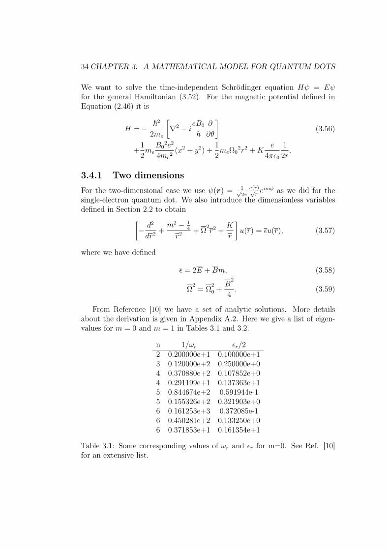
From Reference [10] we have a set of analytic solutions. More detailsabout the derivation is given in Appendix A.2. Here we give a list of eigen-values for m = 0 and m = 1 in Tables 3.1 and 3.2.
n 1/ωr εr/22 0.200000e+1 0.100000e+13 0.120000e+2 0.250000e+04 0.370880e+2 0.107852e+04 0.291199e+1 0.137363e+15 0.844674e+2 0.591944e-15 0.155326e+2 0.321903e+06 0.161253e+3 0.372085e-16 0.450281e+2 0.133250e+06 0.371853e+1 0.161354e+1
Table 3.1: Some corresponding values of ωr and εr for m=0. See Ref. [10]for an extensive list.
3.4. THE TWO-ELECTRON QUANTUM DOT 35
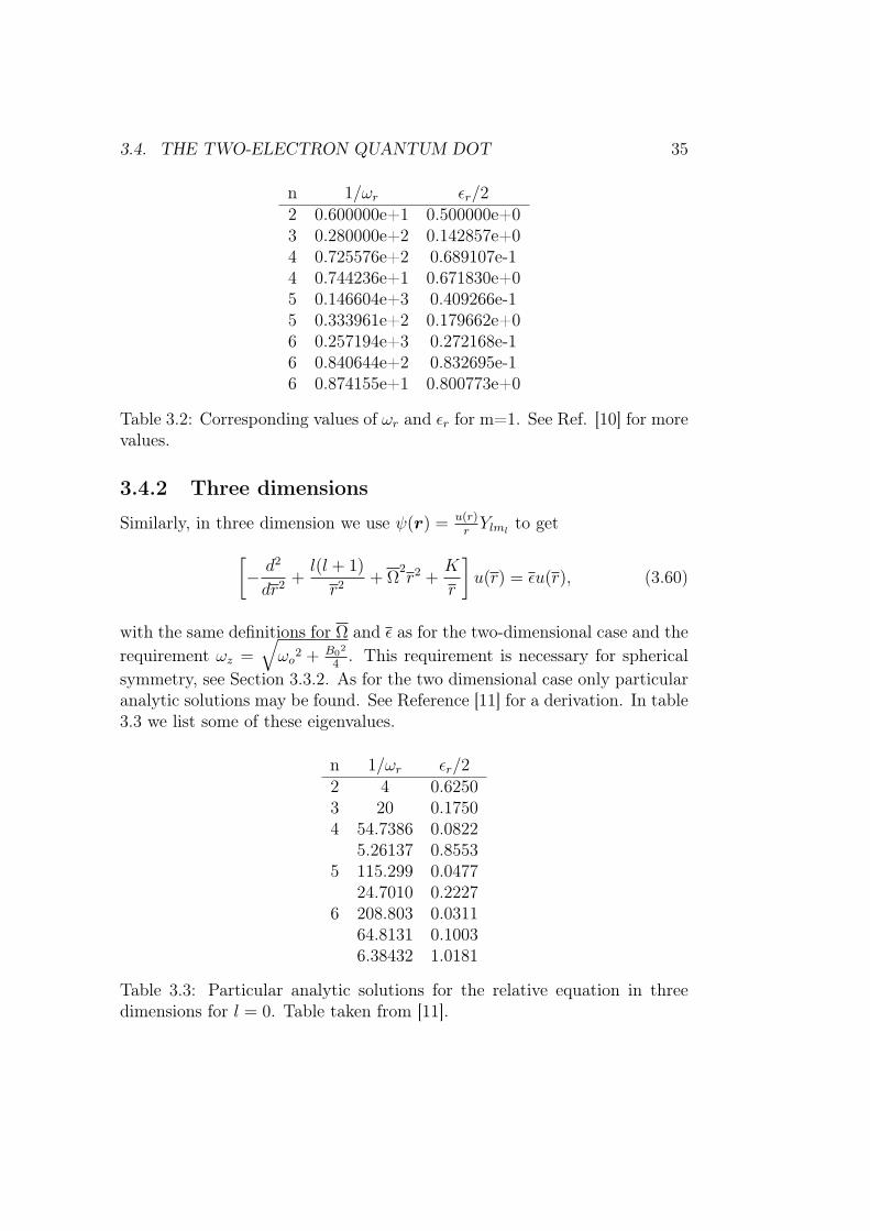
n 1/ωr εr/22 0.600000e+1 0.500000e+03 0.280000e+2 0.142857e+04 0.725576e+2 0.689107e-14 0.744236e+1 0.671830e+05 0.146604e+3 0.409266e-15 0.333961e+2 0.179662e+06 0.257194e+3 0.272168e-16 0.840644e+2 0.832695e-16 0.874155e+1 0.800773e+0
Table 3.2: Corresponding values of ωr and εr for m=1. See Ref. [10] for morevalues.
3.4.2 Three dimensions
Similarly, in three dimension we use ψ(r) = u(r)rYlml
to get[− d2
dr2 +l(l + 1)
r2 + Ω2r2 +
K
r
]u(r) = εu(r), (3.60)
with the same definitions for Ω and ε as for the two-dimensional case and therequirement ωz =
√ωo
2 + B02
4. This requirement is necessary for spherical
symmetry, see Section 3.3.2. As for the two dimensional case only particularanalytic solutions may be found. See Reference [11] for a derivation. In table3.3 we list some of these eigenvalues.
n 1/ωr εr/22 4 0.62503 20 0.17504 54.7386 0.0822
5.26137 0.85535 115.299 0.0477
24.7010 0.22276 208.803 0.0311
64.8131 0.10036.38432 1.0181
Table 3.3: Particular analytic solutions for the relative equation in threedimensions for l = 0. Table taken from [11].
36 CHAPTER 3. A MATHEMATICAL MODEL FOR QUANTUM DOTS
3.4.3 Anti-symmetric wave functions for two particles
When we are working with fermions we require that the total wave functionis anti-symmetric under the interchange of two particles r1 ↔ r2. In our newset of coordinates an interchange means that
R→ R, r → −r.
We observe that the centre-of-mass wave function is always symmetric. Forthe relative coordinates in two dimensions, an interchange of particles gives
r → r, φ→ φ+ π.
The only part of the wave function that changes is eimφ. From this we have
eimφ → eimφeimπ = (−1)meimφ.
For even m the spatial wave function is symmetric, and we must use ananti-symmetric spin function. When m is odd the spatial wave function isanti-symmetric, and we must use a symmetric spin-function. In Section 2.5.2we ordered the four spin states into symmetric (triplet) and anti-symmetric(singlet) states.
3.5 SummaryWe now summarise the equations we have derived in this chapter. From nowon we only use the dimensionless variables defined in Section 2.2. We removeall the overline symbols for the variables and let r → r etc. From the generalequation defined by the Hamiltonian (3.52) we get a radial equation. In twodimensions it is[
− d2
dr2+m2 − 1
4
r2+ Ω2r2 +
K
r
]u(r) = εu(r), (3.61)
and in three dimensions it has a similar form[− d2
dr2+l(l + 1)
r2+ Ω2r2 +
K
r
]u(r) = εu(r). (3.62)
In both equations we have
ε = 2E +Bm, (3.63)
Ω2 = Ω20 +
B2
4. (3.64)
3.5. SUMMARY 37
We can use these equations to solve the single-electron quantum dot, and thecentre-of-mass equation and the relative motion equation for the two-electronquantum dot, where the constants must be defined for each problem by
Single particle: Ω0 = ω0, K = 0, B = B0, (3.65)Centre-of-mass: Ω0 = 2ω0, K = 0, B = 2B0 and (3.66)
Relative motion: Ω0 =1
2ω0, K = 1 B =
1
2B0. (3.67)
The total energy of the two-particle problem is
E = 2Er +1
2ER + 2Φ−BoMs, (3.68)
where Ms = ms1 +ms2 . The energy depend on the quantum numbers
nR = 0, 1, 2, . . . , nr = 0, 1, 2, . . . ,
ms1 = ±1
2, ms2 = ±1
2,
in two dimensions we also have
mR = 0,±1,±2, . . . , mr = 0,±1,±2, . . . ,
and in three dimensions
lR = 0, 1, 2, . . . , lr = 0, 1, 2, . . . ,
mR = 0,±1,±2, . . .± lR, mr = 0,±1,±2, . . .± lR.

Chapter 4
Numerical methods
In this chapter we give the numerical methods used in this thesis. The mainfocus is on solving partial differential equations. We first have a short sectionabout the finite difference method and the finite element method, where wefocus on the finite element method. We also discuss the of parallelisation ofdifferential equations. In this thesis we will solve a one-dimensional equation,therefore we focus on the one-dimensional cases in these methods. In Sec-tion 4.4 we give a special numerical method for solving the time-dependentSchrödinger equation, the Blanes-Moan method. The last part of this chaptergive a short introduction to eigenvalue problems and the ARPACK software.
4.1 Finite difference method (FDM)
In the finite difference method we partition the domain into a grid with Nnodes x0, x1, . . . xN−1. On this grid we search for an approximation ui to theexact solution u(xi) on each node. If the number of nodes is N , then thedistance between the nodes is
h =xmax − xmin
N − 1.
The first derivative is approximated by
dui
dx≈ ui+1 − ui−1
2h. (4.1)
39
40 CHAPTER 4. NUMERICAL METHODS
Using this approximation we calculate the second derivative
d2ui
dx2≈u′i+1/2 − u′i−1/2
h(4.2)
=ui+1 − ui
h2− ui − ui−1
h2
=ui+1 − 2ui + ui−1
h2.
The truncation error can be calculated by a Taylor expansion of u aroundxi±1
ui±1 = ui ± hu′ +h2u′′
2± h3u′′′
6+ . . . .
Using this in Equation 4.2 we have
ui+1 − 2ui + ui−1
h2= u′′ +
h2u(4)
12+h4u(6)
360+O(h6), (4.3)
which gives
d2ui
dx2=ui+1 − 2ui + ui−1
h2+O(h2). (4.4)
The finite difference method approximates the differential equation at thenodes. For a differential operator D we get a matrix: Du→ Au, where u is avector consisting of all the ui in the domain. For simple boundary conditionsof the form u(xk) = f , we write uk = f . Another type of boundary conditioninvolving the derivative u′(xk) = g, can be implemented by the discretisationof the first derivative (4.1) as uk+1 − uk−1 = g, or by another first derivativediscertisation. The boundary conditions are implemented directly on thelinear system, we see show this in the example below.
Example: The Poisson equation
For the Poisson equation
− d2
dx2u(x) = f(x), x ∈ (0, 1), (4.5)
u(0) = 0, u(1) = 0,
we discretise the interior points by
−ui−1 + 2ui − ii+1 = h2f(xi), i = 1, . . . i = N − 2, (4.6)
4.1. FINITE DIFFERENCE METHOD (FDM) 41
and set the boundary conditions as
u0 = 0, uN−1 = 0.
We get a tridiagonal linear system
Au = b,
where
A =
1 0 0 0 . . . 0 0−1 2 −1 0 . . . 0 00 −1 2 −1 0 . . . 0. . . . . . . . . . . . . . . . . . . . .0 . . . . . . . . . . . . 2 −10 . . . . . . . . . . . . 0 1
,
and
b = h2
0f1
f2...
fN−2
0
.
4.1.1 Richardson extrapolation
The approximation to the second derivative given above is on the form
T (h) = T (0) + a1h2 + a2h
4...,
where T (0) is the solution when h→ 0, and a1, a2 . . . are constants indepen-dent of h. For an approximation like this, we can use Richardsons extrapo-lation [12]. The Richardson extrapolations consists of doing approximationsfor different step lengths h, and using these approximations to eliminate errorterms. For example in we calculate T (h) and T (h
2) we can eliminate a1 by
4T (h2)− T (h)
3= T (0)− 1
4a2h
4 + . . . .
We can obtain the formula
T (k)m = T
(k+1)m−1 +
T(k+1)m−1 − T
(k)m−1
4m − 1, m > 0 (4.7)
=4mT
(k+1)m−1 − T
(k)m−1
4m − 1,
42 CHAPTER 4. NUMERICAL METHODS
where T (k)0 = T ( h
2k ), which results in an improved error
T (k)m = T (0) + ak,m
m+1h2(m+1) + ak,m
m+2h2(m+2) + . . . (4.8)
= T (0) +O(h2(m+1)). (4.9)
4.2 Finite element method (FEM)The finite element method (FEM) is more complicated to implement thanthe finite difference method, but it provides a more flexible method to ap-proximate differential equations. For example, the finite element methodcan easily be extended to higher order approximations and can be used forcomplex geometries. We provide a short introduction here, focusing on theone-dimensional case. For a good introductory text to the finite elementmethod see for example Computational Partial Differential Equations [13],or see Reference [14].
4.2.1 One dimensional finite element method
We introduce the finite element method by the following steps:
1. Divide the domain Ω into M non-overlapping elements,
Ωe, e = 1, . . . ,M.
Each element has ne nodes, where the global nodes are denoted by
x[i], i = 1, . . . , N.
The total number of nodes is N = M(ne − 1) + 1 because two neigh-bouring elements share one node. The size of each element he is thedistance between the two boundary nodes of the element.
2. We write our differential equation as
L(u(x)) = 0,
where L is a differential operator specific to our problem.
3. We approximate the function u(x) by:
u(x) ≈ u =N∑
j=1
ujNj(x), (4.10)
where uj are the unknowns and Nj(x) are basis functions.
4.2. FINITE ELEMENT METHOD (FEM) 43
4. We minimise the residual L(u) by∫Ω
L(u)NidΩ = 0, i = 1, . . . , N. (4.11)
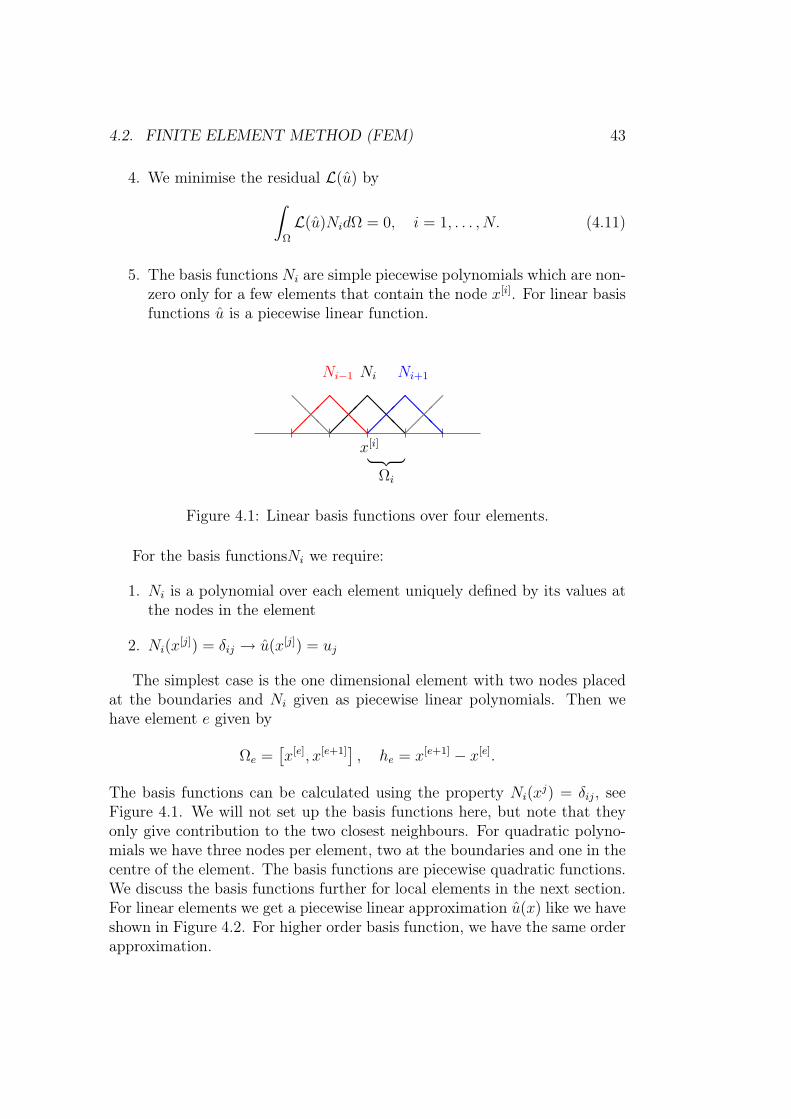
5. The basis functions Ni are simple piecewise polynomials which are non-zero only for a few elements that contain the node x[i]. For linear basisfunctions u is a piecewise linear function.
x[i]
Ωi
Ni
@@
@
Ni+1
@@
@
Ni−1
@@
@
@@
@
Figure 4.1: Linear basis functions over four elements.
For the basis functionsNi we require:
1. Ni is a polynomial over each element uniquely defined by its values atthe nodes in the element
2. Ni(x[j]) = δij → u(x[j]) = uj
The simplest case is the one dimensional element with two nodes placedat the boundaries and Ni given as piecewise linear polynomials. Then wehave element e given by
Ωe =[x[e], x[e+1]
], he = x[e+1] − x[e].
The basis functions can be calculated using the property Ni(xj) = δij, see
Figure 4.1. We will not set up the basis functions here, but note that theyonly give contribution to the two closest neighbours. For quadratic polyno-mials we have three nodes per element, two at the boundaries and one in thecentre of the element. The basis functions are piecewise quadratic functions.We discuss the basis functions further for local elements in the next section.For linear elements we get a piecewise linear approximation u(x) like we haveshown in Figure 4.2. For higher order basis function, we have the same orderapproximation.
44 CHAPTER 4. NUMERICAL METHODS
HHH
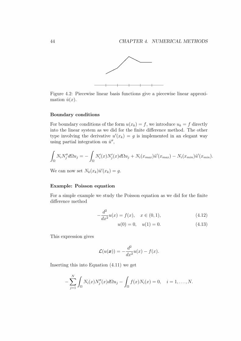
Figure 4.2: Piecewise linear basis functions give a piecewise linear approxi-mation u(x).
Boundary conditions
For boundary conditions of the form u(xk) = f , we introduce uk = f directlyinto the linear system as we did for the finite difference method. The othertype involving the derivative u′(xk) = g is implemented in an elegant wayusing partial integration on u′′,∫
Ω
NiN′′j dΩuj = −
∫Ω
N ′i(x)N
′j(x)dΩuj +Ni(xmax)u
′(xmax)−Ni(xmin)u′(xmin).
We can now set Nk(xk)u′(xk) = g.
Example: Poisson equation
For a simple example we study the Poisson equation as we did for the finitedifference method
− d2
dx2u(x) = f(x), x ∈ (0, 1), (4.12)
u(0) = 0, u(1) = 0. (4.13)
This expression gives
L(u(x)) = − d2
dx2u(x)− f(x).
Inserting this into Equation (4.11) we get
−N∑
j=1
∫Ω
Ni(x)N′′j (x)dΩuj −
∫Ω
f(x)Ni(x) = 0, i = 1, . . . , N.
4.2. FINITE ELEMENT METHOD (FEM) 45
For expressions of the form Ni(x)N′′j (x) we use integration by parts
N∑j=1
∫Ω
N ′i(x)N
′j(x)dΩuj −Ni(xmax)u
′(xmax) +Ni(xmin)u′(xmin)
−∫
Ω
f(x)Ni(x) = 0, i = 1, . . . , N.
The boundary integral terms always give zero contribution for i = 2, . . . , N−1. For our set of boundary conditions (4.13) we also get zero contribution fori = 0 and i = N . We use linear elements. Because of the properties of thebasis functions we only get contributions to the sums for j = (i− 1, i, i+ 1)
i+1∑j=i−1
∫Ω
N ′i(x)N
′j(x)dΩuj −
∫Ω
f(x)Ni(x) = 0, i = 2, . . . , N − 1.
The result is a tridiagonal linear system
i+1∑j=i−1
Aijuj = bi,
where
Aij =
∫Ω
N ′i(x)N
′j(x)dΩ, bi =
∫Ω
f(x)Ni(x).
In addition we must impose the boundary conditions u1 = 0 and uN = 0directly in this linear system. Here we have set up the linear system for thisspecific problem, but a similar construction can be set up for any problem.In general an operator L working on a function u gives a matrix, while afunction independent of u (like f(x)) gives a vector. In this example we endup with a linear system of equations, but we will see in Chapter 5 that foreigenvalue problems we end up with a generalised eigenvalue problem. For aone dimensional problem the matrix will have a bandwidth of 2ne− 1, wherene is the number of nodes per element. For higher dimensions this may notbe the case.
4.2.2 Element-by-element formulation
In this section we introduce the element-by-element formulation. By intro-ducing local coordinates we can generalise the elements regardless of the size
46 CHAPTER 4. NUMERICAL METHODS
and shape of the elements to standard boundaries. Following the examplefrom the previous section we write a sum over each element e
Aij =M∑
e=1
A(e)ij , A
(e)ij =
∫Ωe
N ′iN
′jdΩ and (4.14)
bi =M∑
e=1
b(e)i , b
(e)i =
∫Ωe
NifdΩ. (4.15)
We define the matrix A(e)ij as an element matrix, and b
(e)i as an element
vector, note that the integrals above depend on the problem we are solving.In element e, A(e)
ij is different from zero only for the nodes that belong to thiselement. Therefore the element matrix/vector has the size ne.
We now define local coordinates and numbering of nodes. We choose thelocal coordinate
ξ ∈ [−1, 1],
and define local node numbers
r, s = 1, . . . , ne,
that map to the global node numbers i, j by i = q(e, r) and j = q(e, s). Forthe one-dimensional case we have the simple expression
q(e, r) =(ne − 1)(e− 1) + r, (4.16)e = 1, . . . ,M, r = 1, . . . , ne, q = 1, . . . , N,
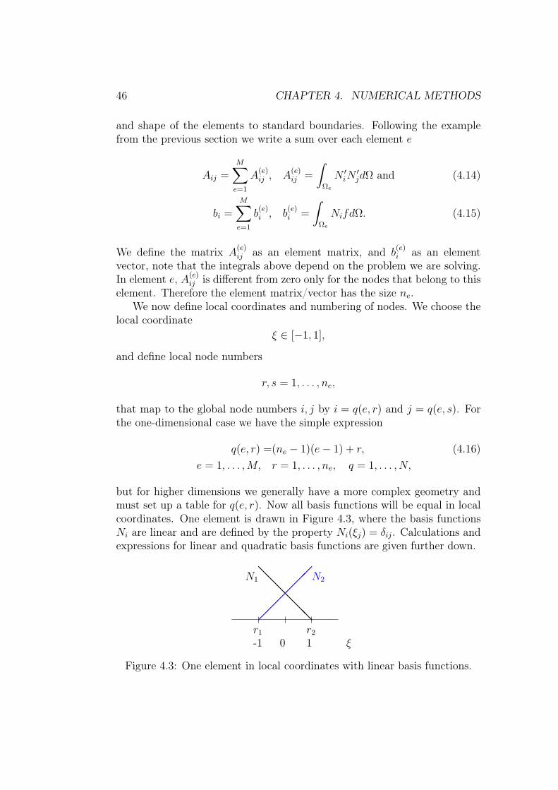
but for higher dimensions we generally have a more complex geometry andmust set up a table for q(e, r). Now all basis functions will be equal in localcoordinates. One element is drawn in Figure 4.3, where the basis functionsNi are linear and are defined by the property Ni(ξj) = δij. Calculations andexpressions for linear and quadratic basis functions are given further down.
r1 r2-1 0 1 ξ
N1@
@@
@@
@
N2
Figure 4.3: One element in local coordinates with linear basis functions.
4.2. FINITE ELEMENT METHOD (FEM) 47
We map from global coordinates x to local coordinates ξ by
x(e)(ξ) =ne∑
r=1
Nr(ξ)xq(e,r), (4.17)
where Nr(ξ) are the basis functions defined for local coordinates (expressionsare given on the next page ). The derivatives transform as
dNi
dx=dNr
dξ
dξ
dx= J−1dNr
dξ, (4.18)
dNj
dx=dNs
dξ
dξ
dx= J−1dNs
dξ, (4.19)
where r, s are local node numbers corresponding to i = q(e, r) and j = q(e, s).The integral is given by ∫ x[e+1]
x[e]
dx =
∫ 1
−1
detJdξ, (4.20)
where J is defined asJi,j =
∂xj
∂ξj,
in the case of one-dimensional piecewise linear basis functions J has thesimple form J = he
2.
After calculating the integrals each element will have it’s own ne × ne
element matrix and element vector of size ne given by A(e) with matrix el-ements A(e)
rs , and element vector b(e) with b(e)r . We assemble the element
matrices/vectors by adding them to the global system using i = q(e, r) tofind the correct global nodes
Aq(e,r),q(e,s)+ = A(e)r,s ,
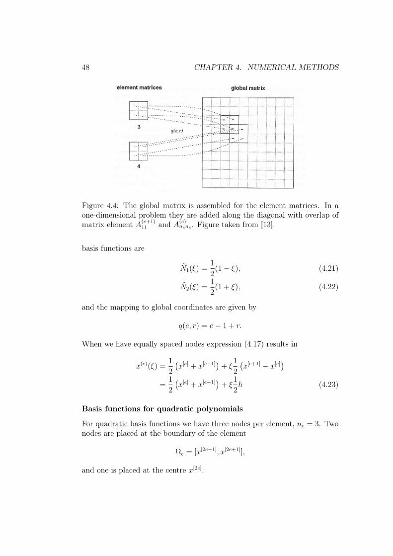
bq(e,r)+ = b(e)r .
For the matrix case this is shown in Figure 4.4. For the one dimensional casewe see that we get an overlap of matrix element A(e+1)
11 and A(e)nene . The same
goes for the element vectors, we get an overlap of b(e+1)1 and b(e)ne .
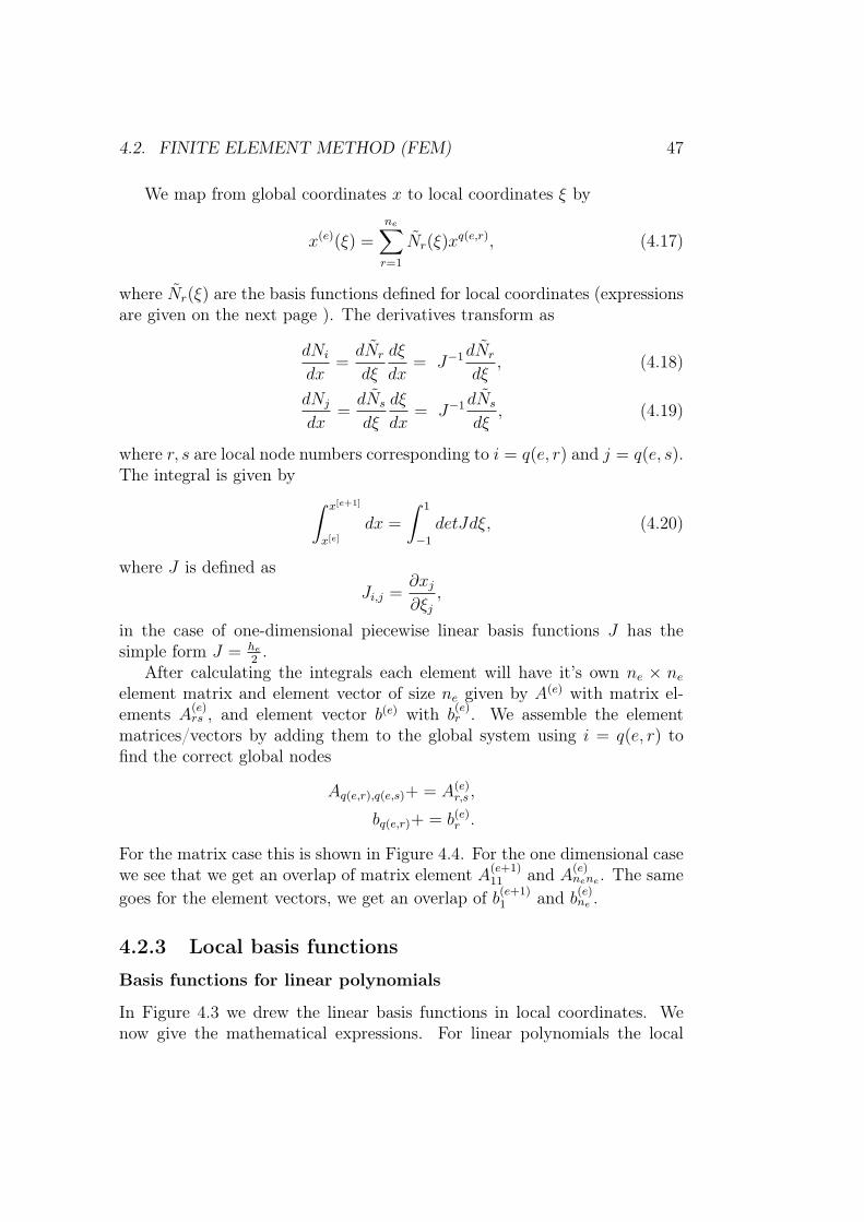
4.2.3 Local basis functions
Basis functions for linear polynomials
In Figure 4.3 we drew the linear basis functions in local coordinates. Wenow give the mathematical expressions. For linear polynomials the local
48 CHAPTER 4. NUMERICAL METHODS
Figure 4.4: The global matrix is assembled for the element matrices. In aone-dimensional problem they are added along the diagonal with overlap ofmatrix element A(e+1)
11 and A(e)nene . Figure taken from [13].
basis functions are
N1(ξ) =1
2(1− ξ), (4.21)
N2(ξ) =1
2(1 + ξ), (4.22)
and the mapping to global coordinates are given by
q(e, r) = e− 1 + r.
When we have equally spaced nodes expression (4.17) results in
x(e)(ξ) =1
2
(x[e] + x[e+1]
)+ ξ
1
2
(x[e+1] − x[e]
)=
1
2
(x[e] + x[e+1]
)+ ξ
1
2h (4.23)
Basis functions for quadratic polynomials
For quadratic basis functions we have three nodes per element, ne = 3. Twonodes are placed at the boundary of the element
Ωe = [x[2e−1], x[2e+1]],
and one is placed at the centre x[2e].
4.2. FINITE ELEMENT METHOD (FEM) 49
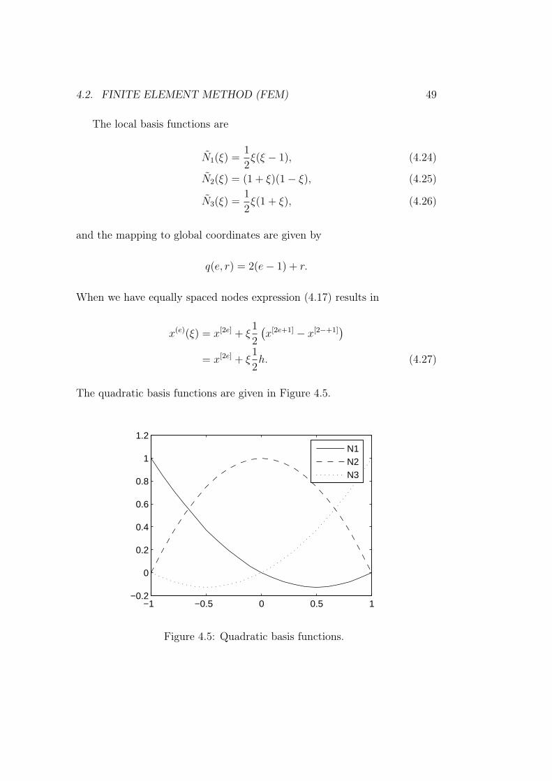
The local basis functions are
N1(ξ) =1
2ξ(ξ − 1), (4.24)
N2(ξ) = (1 + ξ)(1− ξ), (4.25)
N3(ξ) =1
2ξ(1 + ξ), (4.26)
and the mapping to global coordinates are given by
q(e, r) = 2(e− 1) + r.
When we have equally spaced nodes expression (4.17) results in
x(e)(ξ) = x[2e] + ξ1
2
(x[2e+1] − x[2−+1]
)= x[2e] + ξ
1
2h. (4.27)
The quadratic basis functions are given in Figure 4.5.
−1 −0.5 0 0.5 1−0.2
0
0.2
0.4
0.6
0.8
1
1.2
N1N2N3
Figure 4.5: Quadratic basis functions.
50 CHAPTER 4. NUMERICAL METHODS
Calculation of local basis functions
We require that the basis functions have the property Ni(ξj) = δij. For thefirst linear basis function we have
Ni(ξ) = aξ + b,
N1(−1) = 1 = −a+ b,
N1(1) = 0 = a+ b,
which gives the linear system for a and b[−1 11 1
] [ab
]=
[10
].
Compactly, we write the two linear systems for N1 and N2 as[−1 11 1
] [ab
]=
[δi1δi2
].
The solution for the basis functions are
N1(ξ) =1
2− 1
2ξ,
N2(ξ) =1
2+
1
2ξ.
Similarly, for quadratic elements we have the linear systems 1 −1 10 0 11 1 1
abc
δi1δi2δi3
We now have three linear systems to solve, resulting in (4.24) - (4.26). Thesame procedure can be done for higher order polynomials.
4.2.4 Algorithm
To get an overview of a finite element algorithm we set it up for the Poissonexample (4.12) here. However this algorithm can be generalised using otherelement vectors/matrices than br and Ars. For example in the quantum dotequation we get two element matrices and no element vector.
4.2. FINITE ELEMENT METHOD (FEM) 51
FINITE ELEMENT ALGORITHMInitialise gridset global and element matrices/vectors = 0for e=1, . . . ,m LOOP OVER ALL ELEMENTS
for r,s=1, . . . , ne LOOP OVER LOCAL NODESCalculate the integrals for the local element matrices/vectors (Ars and br)
Set essential boundary conditonsAdd the local element matrix A(e) and vector b(e) to the global system
Solve the resulting linear system
4.2.5 Higher dimensions
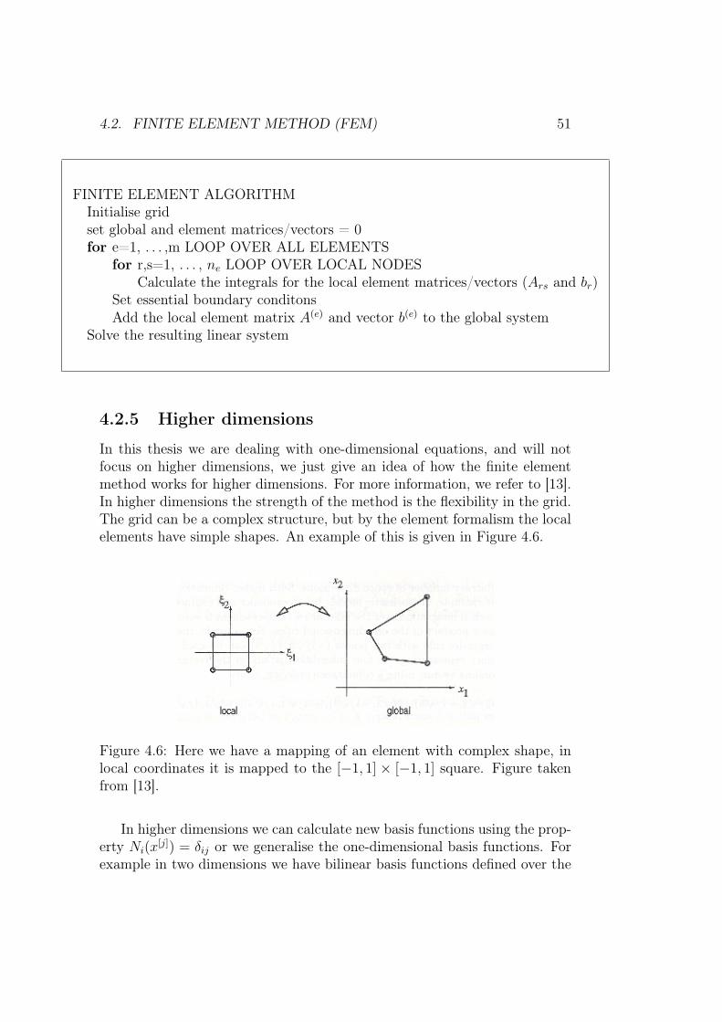
In this thesis we are dealing with one-dimensional equations, and will notfocus on higher dimensions, we just give an idea of how the finite elementmethod works for higher dimensions. For more information, we refer to [13].In higher dimensions the strength of the method is the flexibility in the grid.The grid can be a complex structure, but by the element formalism the localelements have simple shapes. An example of this is given in Figure 4.6.
Figure 4.6: Here we have a mapping of an element with complex shape, inlocal coordinates it is mapped to the [−1, 1] × [−1, 1] square. Figure takenfrom [13].
In higher dimensions we can calculate new basis functions using the prop-erty Ni(x
[j]) = δij or we generalise the one-dimensional basis functions. Forexample in two dimensions we have bilinear basis functions defined over the
52 CHAPTER 4. NUMERICAL METHODS
rectangle [−1, 1]× [−1, 1] by
N1(ξ1, ξ2) = N1(ξ1)N1(ξ2),
N2(ξ1, ξ2) = N2(ξ1)N1(ξ2),
N3(ξ1, ξ2) = N1(ξ1)N2(ξ2),
N4(ξ1, ξ2) = N2(ξ1)N2(ξ2).
The assembly of the global linear system for higher dimensions is more com-plicated and we have to make sure to add the contribution to a node fromall the elements containing that node.
4.2.6 Time-dependent problems
For time-dependent problems it is most common to use the finite elementmethod for discretisation in space and the finite difference method for dis-cretisation in time. If we denote the time step as ul = u(x, tl) we discretisethe time derivative by a finite difference scheme and then apply the finiteelement discretisation
ul(x) ≈ ul =N∑
j=1
uljNj(x). (4.28)
We show this on a simple example
du
dt= Lu.
We discertise this using the Euler method in time dudt≈ ul+1−ul
∆tand get
ul+1 = ul + ∆tLul.
We now introduce the discretisation (4.28) and obtain∫Ω
NiNjdΩul+1j =
∫Ω
NiNjdΩulj + ∆t
∫Ω
NiLNjdΩulj, (4.29)
→ Aul+1 = Aul + ∆tBul, (4.30)
when we write out the matrices. This gives a linear system to be solved foreach time step. We discuss some special numerical methods for the evolutionof the time-dependent Schrödinger equation in 4.4.
4.3. SOLVING PARTIAL DIFFERENTIAL EQUATIONS IN PARALLEL53
4.3 Solving partial differential equations in par-allel
The capacity of single processors can no longer keep up with the demand forlarger and faster simulations in scientific computing. To meet these increasingdemands we need parallel computing. In parallel computing we divide thework among a number of processors to run larger and faster simulations.The memory on a multiple processor computer can be organised in severalways. The most common way is the distributed memory system, where eachprocessor has its own memory. For such systems data must be exchangedexplicitly by message passing. MPI - “message passing interface” is a usefullibrary which provides functions for communication between processors.Thismust be provided by the programmer. Because of communication cost dueto message passing a parallel program will not acquire full speed-up
S(P ) =T (1)
T (P )≤ P. (4.31)
Here T (i) is the time spent using i processors and P is the number of proces-sors in parallel. The partitioning of the work is dependent on the algorithm.For an efficient parallel algorithm the work load should be evenly distributedto avoid idle time, and the communication cost should be minimised. In thisthesis we focus on parallelisation of partial differential equations (PDE).
When solving a PDE there are two time consuming parts: building thematrices/vectors in the system and solving this system (linear system oreigenvalue problem). The first step is to partition the data among the pro-cessors. In most cases the spatial grid is divided into P sub grids. Eachprocessor only has access to its own sub grid data. On this sub grid the pro-cessor applies operations in the same way as a sequential solver. In additionwe provide communication between neighbouring sub grids. After reviewingthe linear system and linear algebra operations we give more details of thepartitioning of finite difference grid and finite element grids.
To solve a linear system or an eigenvalue problem in parallel we mustuse iterative solvers. Iterative solvers generally rely on the linear algebraoperations: matrix-vector product, vector addition and the inner product.The task of parallelising an iterative solver thus consists of parallelising theseoperations according to the partitioning of the matrices and vectors.
54 CHAPTER 4. NUMERICAL METHODS
4.3.1 Parallel linear algebra operations
In a matrix the rows are partitioned
A =
A11 A12 · · · A1P
A21 A22 · · · A2P...
... . . . ...AP1 AP2 · · · APP
, (4.32)
where Aij are block matrices. Processor p holds the blocks Aip. The linesdivide the matrix/vector among the processors. For a vector we have
b =
b1
b2
...bP
. (4.33)
From this partitioning we set up the linear algebra operations:
Vector addition
The vector addition w = x+ y is given by local vector additions
wp = xp + yp, p = 1, . . . , P. (4.34)
This operation requires no communication.
Inner product
The inner product s = x · y is calculated locally on each processor p by
sp = xp · yp. (4.35)
All the local inner products sp are sent to a master node where the fullinner product is calculated s =
∑P1 sp (or distributed to all processors using
MPI_ALLREDUCE with MPI_SUM).
Matrix-vector product
The matrix-vector product w = Ab requires communication between allprocessors for a full matrix A. However when we discretise a PDE, thematrix is sparse. By using a smart partitioning, many of the block matricesare zero and we only need communication between a few processors.
4.3. SOLVING PARTIAL DIFFERENTIAL EQUATIONS IN PARALLEL55
Using the definitions above the result should be
w =
w1 = A11b1 + A12b2 + . . . A1PbP
w2 = A21b1 + A22b2 + . . . A2PbP
...wP = AP1b1 + AP2b2 + . . . APPbP
.From these expressions we see that we can calculate local matrix-vector prod-ucts. The local result Appbp is stored in wp, while the array Apqbq is sent toprocessor q and added to the vector wq.
4.3.2 Grid partitioning
Partitioning of finite difference grids
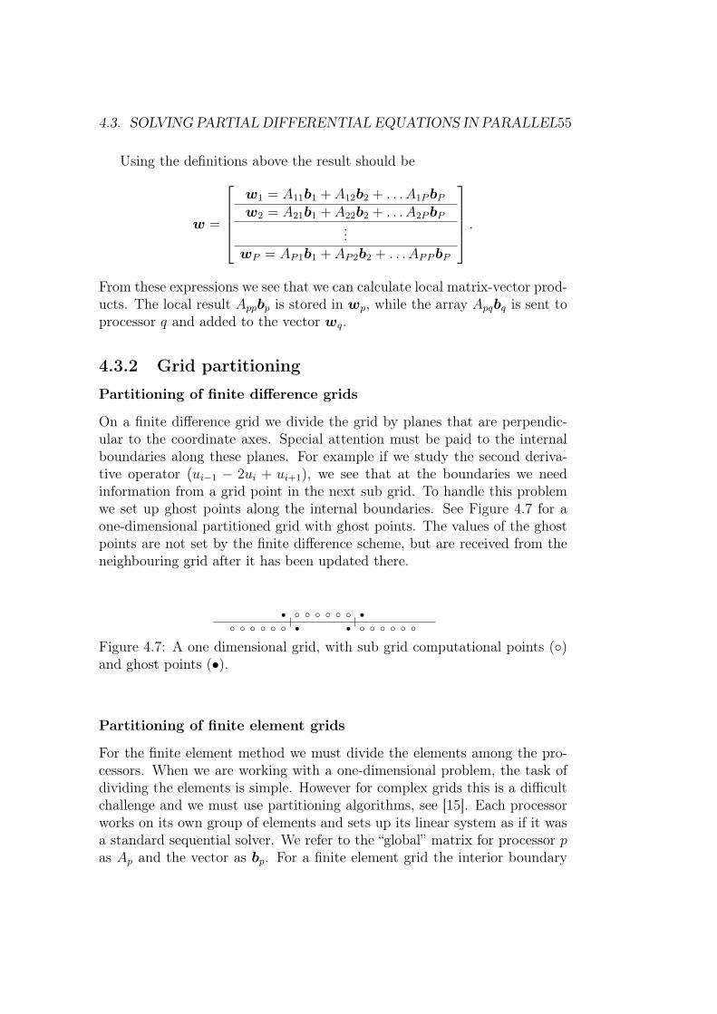
On a finite difference grid we divide the grid by planes that are perpendic-ular to the coordinate axes. Special attention must be paid to the internalboundaries along these planes. For example if we study the second deriva-tive operator (ui−1 − 2ui + ui+1), we see that at the boundaries we needinformation from a grid point in the next sub grid. To handle this problemwe set up ghost points along the internal boundaries. See Figure 4.7 for aone-dimensional partitioned grid with ghost points. The values of the ghostpoints are not set by the finite difference scheme, but are received from theneighbouring grid after it has been updated there.
b b b b b br rb b b b b br b b b b b brFigure 4.7: A one dimensional grid, with sub grid computational points ()and ghost points (•).
Partitioning of finite element grids
For the finite element method we must divide the elements among the pro-cessors. When we are working with a one-dimensional problem, the task ofdividing the elements is simple. However for complex grids this is a difficultchallenge and we must use partitioning algorithms, see [15]. Each processorworks on its own group of elements and sets up its linear system as if it wasa standard sequential solver. We refer to the “global” matrix for processor pas Ap and the vector as bp. For a finite element grid the interior boundary
56 CHAPTER 4. NUMERICAL METHODS
points are shared between two (or more in higher dimensions) sub grids, be-cause of this Ap and bp will not be equal to A and b at the interior boundarynodes. For a vector bi we sum the values at the shared boundary nodes, sothat all the boundary nodes have the correct (and same) value. This specialconstruction affects the linear algebra operations.
The vector addition is the same. For the finite element method the bound-ary nodes are duplicated and local inner product must be adjusted by
ci = ci −∑
k
ok − 1
ok
ukvk, (4.36)
where k runs over all internal boundary nodes and ok is the number of subgrids sharing this node. In the one-dimensional case each internal boundarynode belong to two processors and have ok = 2. The matrix-vector productis simplified. First we calculate the local matrix vector products wi = Aiui.To get the correct values and the internal boundaries we add the contributionfrom all the neighbouring sub grids for wi.
4.4 Time evolution of the Schrödinger equationThe time-dependent Schrödinger equation is
i~∂
∂tψ(t) = H(t)ψ(t), (4.37)
where ψ is also a function of the spatial coordinates, but for simplicity wejust write the time coordinate here. We define the time evolution operatorU by
ψ(t2) = U(t2, t1)ψ(t1), ψ(t) = U(t, 0)ψ(0), (4.38)
and rewrite the Schrödinger equation into an equation for U
i~∂
∂tU(t) = H(t)U(t). (4.39)
For a time-independent Hamiltonian the time evolution operator is U(t) =e−iEt/~, where E is a diagonal matrix with the eigenvalues along the diagonal.To avoid working with imaginary numbers we can use imaginary time t = iτ ,we also use atomic units as defined in Section 2.2. The equation for U is then
∂
∂τU(τ) = H(τ)U(τ) (4.40)
4.4. TIME EVOLUTION OF THE SCHRÖDINGER EQUATION 57
Using a simple Euler scheme we have
∂
∂τ≈ ul+1 − ul
∆τ, (4.41)
→ ul+1 =[1 + ∆τH l
]ul, (4.42)
with ul = U(τ) and H l = H(τ). A more accurate finite difference scheme isthe Runge-Kutta method. It has an accuracy of O(h5), where h is the steplength. The next time step is calculated by
k1 = hH lul, (4.43)
k2 = hH l(ul +1
2k1), (4.44)
k3 = hH l(ul +1
2k2), (4.45)
k4 = hH l(ul + k3), (4.46)
ul+1 = ul +1
6(k1 + 2k2 + 2k3 + k4). (4.47)
Here ki are also vectors of the same size as u.
4.4.1 Splitting of the Hamiltonian
We write the Hamiltonian on the form
H = H0 +H1(t), (4.48)
where H0 is time-independent. If we solve the time-independent Schrödingerequation for H0, as we have done for the quantum dot in Chapter 3, we cando a change of basis
H0 = PEP †, (4.49)
where E is a diagonal matrix with the eigenvalues of H0 on the diagonal,and P is a unitary matrix where the columns are the eigenvectors. We alsodefine
d(t) = P †u(t) and W (t) = P †H1(t)P. (4.50)
If we apply P † on H lul we have
P †H lul = P †H0ul + P †H l
1ul (4.51)
= EP †ul +W lP †ul (4.52)=
[E +W l
]dl. (4.53)
58 CHAPTER 4. NUMERICAL METHODS
4.4.2 Blanes-Moan method
When we have a separable Hamiltonian we can use the Blanes-Moan methoddescribed in [16]. In this article another splitting is defined, but we use thesplitting defined in Equation (4.48). We approximate the time evolutionoperator by discretising the total time interval (0, t) into Nt steps
U(t, 0) =U(t1, t0)U(t2, t1) · · ·U(tNt , tNt−1) (4.54)
=Nt−1∏n=0
U(tn + ∆t, tn), (4.55)
where
∆t =t
Nt
, tn = n∆τ, n = 0 . . . , Nt − 1. (4.56)
For a separable Hamiltonian H = A + B the solution can be approximatedby
U = eA1∆t/2eB 1
2∆teA0∆t/2 +O(∆t3), (4.57)
Ak = −iA(tn + k∆t), B 12
= −iB(tn +1
2∆t), k = 1, 2. (4.58)
If we choose to use the basis we defined above and set A = E and B = Wwe have
U = e−iE∆t/2e−i∆tW (tn+ 12∆t)e−iE∆t/2 +O(∆t3), (4.59)
where the expressions are simplified because E is independent of time. Theexponential e−iE∆t/2 is diagonal because E is a diagonal matrix.
A higher precision formula is also defined in [16], where U as approximatedby
U = eH(1)
eH(0)
e−H(1)
+O(∆t5), (4.60)
H(k) = − i
∆tk
∫ tn+∆t
tn
[s−
(tn +
1
2∆t
)]k
H(s)ds, k = 1, 2. (4.61)
Writing out the integrals we have
H(0) = −i∫ tn+∆t
tn
H(s)ds, (4.62)
H(1) = − i
∆t
∫ tn+∆t
tn
[s− tn −
1
2∆t
]H(s)ds
=i
∆t
[tn +
1
2∆t
] ∫ tn+∆t
tn
H(s)ds− i
∆t
∫ tn+∆t
tn
sH(s)ds. (4.63)
4.5. EIGENVALUE PROBLEMS 59
Here we also use the splitting of the Hamiltonian H = E+W (t) for H(k).This simplify the integrals because E is time-independent and go outside theintegrals.∫ tn+∆t
tn
H(s)ds = E∆t+
∫ tn+∆t
tn
W (s)ds, (4.64)∫ tn+∆t
tn
sH(s)ds = E∆t
(tn +
1
2∆t
)+
∫ tn+∆t
tn
sW (s)ds. (4.65)
4.5 Eigenvalue problemsThe time-dependent Schrödinger equation is a differential equation whichmust be solved as an eigenvalue problem. We are searching for the eigenstatesof the Hamiltonian which is a differential operator
Hψ = Eψ. (4.66)
In the previous sections we have discussed the discretisation of differentialequations. When discretising (4.66) we get a matrix eigenvalue problem. Forthe finite difference method we have a standard eigenvalue problem
Au = λu, (4.67)
and for the finite element method we have a generalised eigenvalue problem
Au = λBu. (4.68)
The reason that we get Bu on the right side is that for the finite elementmethod a vector give u→ Bu.
In the special case where B is a symmetric positive definite matrix wecan reduce the generalised eigenvalue problem to a standard one. We do aCholesky decomposition of B
B = LLT ,
and rewrite our problem to(L−1AL−T
) (LTu
)= λ
(LTu
)→ Cy = λy,
which is a standard eigenvalue problem.The standard way to solve eigenvalue problems is by solving the equation
det(A− λI) = 0, (4.69)
60 CHAPTER 4. NUMERICAL METHODS
for λ and solving the linear systems
(A− λiI)xi, (4.70)
for the eigenvectors xi. However this method is not suitable for large prob-lems.
4.5.1 The ARPACK eigenvalue solver
There are several numerical methods for solving a standard eigenvalue prob-lem, such as the Jacobi method, see for example Reference [17]. We will how-ever use the ARPACK software [18]. The ARPACK library provides solversfor both the standard eigenvalue problem and the generalised eigenvalueproblem. There is also a parallel extension: P_ARPACK. The ARPACKsoftware uses the implicitly restarted Arnoldi method. It is an iterativesolver which requires the computation of matrix-vector products. For moredetails about the software package, see the ARPACK user guide [18], and fornumerical methods, see Reference [19]. We will discuss how this package isimplemented in Chapter 5.
Chapter 5
Implementation of the numericalmethods
In this chapter we discuss the implementation of the numerical methods.First we focus on the time-independent Schrödinger equation
H0ψ = Eψ. (5.1)
In Section 5.1 we give the finite element and finite difference discretisationsof the quantum dot equations. We have built a general solver using thesemethods. Details about the program are given in Section 5.2. Then, inSection 5.3, we move on to the time-dependent Schrödinger equation wherethe Hamiltonian is given by
H = H0 +H1(t), (5.2)
whereH0 is the time-independent Hamiltonian which has already been solvedandH1(t) is a time-dependent perturbation. We use the Blanes-Moan method,which was described in Section 4.4. Because we already have a set of eigenval-ues and eigenvectors for H0 we use them as a basis to simplify the equations.
5.1 Implementation of the radial equationIn Chapter 3 we discussed the quantum system for the one-electron andthe two-electron quantum dot. There we derived a general one-dimensionalequation which describes this system. We choose to write it in a more generalform as
− d2u(r)
dr2+ Y (r)u(r) = εu(r), (5.3)
61
62CHAPTER 5. IMPLEMENTATION OF THE NUMERICAL METHODS
where Y (r) = Dr2 + 2V includes both the potential and the constants from
the angular equation
2D: Y (r) =m2 − 1
4
r2+ 2V , (5.4)
3D: Y (r) =l(l + 1)
r2+ 2V . (5.5)
For the quantum dot the potential is
2V = Ω2r2 +K
r, (5.6)
where the constants depend on the problem to be solved: single-electronquantum dot (3.65); two-electron centre-of-mass (3.66); two-electron relative-coordinates (3.67).
The boundary conditions are
u(0) = 0, u(∞) = 0. (5.7)
We must approximate ∞ by a finite value rmax. This value must be largeenough to not influence the results. This is further described in Section 5.2.
After we have discretised the Schrödinger equation using either the finiteelement method or the finite difference method, we get an eigenvalue problem
Au = εBu, (5.8)
where A and B (B=I for FDM) are matrices. We are searching for the eigen-values ε and eigenvectors u(r). Implementation of boundary conditions foreigenvalue problem are more complicated than for a standard linear system,this is discussed in Section 5.1.3. The eigenvalue problems are solved usingARPACK++[18].
5.1.1 Finite difference equations
We discretise the grid by
ri = ih ui = ψ(ri) h =1
N − 1i = 0, 1, ...N − 1,
where N is the number of points. For the second derivative we have
∂2
∂r2ui '
ui−1 − 2ui + ui+1
h2+O(h2).
5.1. IMPLEMENTATION OF THE RADIAL EQUATION 63
Using this approximation in Equation (5.3) we get a tridiagonal matrix eigen-value problem for the interior points and simple boundary conditions
−ui−1 + ui
(2 + Y (ih)h2
)− ui+1 = εh2ui, i = 1..N − 2, (5.9)
u0 = 0, (5.10)uN−1 = 0. (5.11)
For the two-dimensional quantum dot we have for interior points
− ui−1 + ui
(2 +
m2 − 14
i2+Kh
i+ ω2i2h4
)(5.12)
− ui+1 = εh2ui, i = 1, . . . , i = N − 2.
The finite difference method is simple to implement. We build a tridiag-onal matrix
A =
2 + Y1 −1 0 0 . . . 0 0−1 2 + Y2 −1 0 . . . 0 00 −1 2 + Y3 −1 0 . . . 0. . . . . . . . . . . . . . . . . . . . .0 . . . . . . . . . . . . 2 + YN−3 −10 . . . . . . . . . . . . −1 2 + YN−2
,
where Yi = Y (ih)h2 =m2− 1
4
i2+ Kh
i+ω2i2h4. The implementation of boundary
conditions are described in Section 5.1.3. The eigenvalue problem is
Au = εh2u. (5.13)
5.1.2 Finite element equations
We use the flexible element-by-element formulation of the finite elementmethod as described in Section 4.2.2. Here we give the mathematical cal-culations, in Section 5.2 we give more details about how the algorithm isimplemented in the program.
For the general Equation (5.3), we set up local elements. The secondderivative term gives
−d2u(r)
dr2→−
N∑j=1
∫ rmax
0
Ni(r)d2
dr2Nj(r)druj =
N∑j=1
∫ rmax
0
dNi
dr
dNj
drdruj
The element matrix T (e) arising from this term is
T (e)rs =
2
he
∫ 1
−1
dNr
dξ
dNs
dξdξ. (5.14)
64CHAPTER 5. IMPLEMENTATION OF THE NUMERICAL METHODS
Here we have omitted the boundary terms arising from the partial integrationbecause of the boundary conditions u(0) = 0 and u(rmax) = 0. For thisexpression and the following r, s = 1, . . . ne and T
(e)rs are the elements of the
ne × ne matrix T (e). The potential term Y (r) gives
Y (r)u(r) →N∑
j=1
∫ rmax
0
NiY (r)Njdr, (5.15)
which gives another element matrix contribution Y (e)
Y (e)rs =
he
2
∫ 1
−1
NrY (r(ξ))Nsdξ, (5.16)
where we must use r(ξ) as defined in (4.17) for Y (r(ξ)). For the globalmapping we have q(e, s) = (ne − 1)(e − 1) + s, which gives the positions ofthe global nodes as
rq = rmin + (q − 1)h
ne − 1
= rmin + (e− 1)h+s− 1
ne − 1h, (5.17)
q = 1, . . . , N, s = 1, . . . , ne, e = 1, . . .M.
Knowing this expression we calculate r(ξ) as in (4.17). On the right side wehave
εu(r) → εN∑
j=1
∫ rmax
0
NiNjdr, (5.18)
which also gives an element matrix M (e)
εM (e)rs = ε
he
2
∫ 1
−1
NrNsdξ. (5.19)
The global matrices are built by adding up the element matrices as de-scribed in Section 4.2.2. Building the global system we get a generalisedeigenvalue problem
N∑e=1
(T (e) + V (e)
)u = ε
N∑e=1
M (e)u (5.20)
(Au = εBu) ,
5.1. IMPLEMENTATION OF THE RADIAL EQUATION 65
where A and B are the global matrices defined by
A =N∑
e=1
(T (e) + V (e)
), B =
N∑e=1
M (e). (5.21)
Boundary conditions and eigenvalue solvers are discussed in the next section.In the one-dimensional case the matrices are banded with bandwidth 2ne−1.
5.1.3 Boundary conditions for eigenvalue problems
To impose boundary conditions on an eigenvalue problem is more complicatedthat for a simple linear system of equations, which arise from a standarddiscretisation of a differential equation. The generalised eigenvalue problemis
Au = λBu. (5.22)
For the finite difference method we have B = I, which reduces the problemto a standard eigenvalue problem. We define a projection matrix P
P : Cn → Cn−c,
where c is the number of boundary conditions and P is a (n− c)× n matrixwhich is identical to the identity matrix In with row number j removed forboundary nodes xj. The transformation due to P on a vector and a matrixis given by
v = Pu,
X = PXP T .
The effect of this transformation is that the boundary nodes are removedfrom the vector u to form v, and the boundary rows/columns are removedfrom X. The reduced eigenvalue problem is
Av = λBv. (5.23)
This derivation is taken from [20].For the boundary conditions in our problem we remove the first and last
columns/row from the matrices, giving a (N−2)×(N−2) eigenvalue problem.If we want to use the full vector we simply add a zero entry before and afterthe calculated eigenvector, the missing eigenvalues have the value λ = 0.
For the finite difference method this is simple to implement when we setup the matrix because we can omit the boundary nodes from the loop anddirectly set up a (N − 2)× (N − 2) matrix. For the finite element method itis more complicated. We first build the full global matrices and then removethe rows/columns from the matrices.
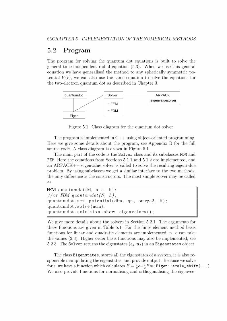
66CHAPTER 5. IMPLEMENTATION OF THE NUMERICAL METHODS
5.2 ProgramThe program for solving the quantum dot equations is built to solve thegeneral time-independent radial equation (5.3). When we use this generalequation we have generalised the method to any spherically symmetric po-tential V (r), we can also use the same equation to solve the equations forthe two-electron quantum dot as described in Chapter 3.
quantumdot Solver
− FEM
− FDM
Eigen
eigenvaluesolver
ARPACK
Figure 5.1: Class diagram for the quantum dot solver.
The program is implemented in C++ using object-oriented programming.Here we give some details about the program, see Appendix B for the fullsource code. A class diagram is drawn in Figure 5.1.
The main part of the code is the Solver class and its subclasses FDM andFEM. Here the equations from Sections 5.1.1 and 5.1.2 are implemented, andan ARPACK++ eigenvalue solver is called to solve the resulting eigenvalueproblem. By using subclasses we get a similar interface to the two methods,the only difference is the constructors. The most simple solver may be calledas:
FEM quantumdot (M, n_e , h) ;//or FDM quantumdot (N, h ) ;quantumdot . s e t_poten t i a l (dim , qn , omega2 , K) ;quantumdot . s o l v e (num) ;quantumdot . s o l u l t i o n . show_eigenvalues ( ) ;
We give more details about the solvers in Section 5.2.1. The arguments forthese functions are given in Table 5.1. For the finite element method basisfunctions for linear and quadratic elements are implemented; n_e can takethe values (2,3). Higher order basis functions may also be implemented, see5.2.3. The Solver returns the eigenstates (ελ,uλ) in an Eigenstates object.
The class Eigenstates, stores all the eigenstates of a system, it is also re-sponsible manipulating the eigenstates, and provide output. Because we solvefor ε, we have a function which calculates E = 1
2ε−1
2Bm; Eigen::scale_shift(...).
We also provide functions for normalising and orthogonalising the eigenvec-
5.2. PROGRAM 67
constructorM number of elementsn_e number of nodes per elementN number of nodesh step lengthset_potentialdim dimensions (2,3)qn quantum number (m in 2D, l in 3D)ω2 scaled oscillator frequencyK strength of electron-electron interaction termsolvenum number of eigenvalues to be found
Table 5.1: Input variable for the solver class.
tors. Some of the available functions are given in Table 5.2. A simple matrixclass has also been implemented.
show_eigenvalues() prints the eigenvalues to screenprint(filename, m, omega) print to file for the matlab script on file.mscale(scale), scales the eigenvalues (E = 1
2ε)
shift(shift), shifts the eigenvalues (E = ε− 12Bm)
scale_shift(scale, shift) scales/shifts the eigenvalues (E = 12ε− 1
2Bm)
normalise() normalise all the eigenvectorsorthogonalise_set() orthonormalise the eigenvectors
Table 5.2: Available functions in the Eigenstates class. The functions ma-nipulate the set of eigenstates and print information. These functions arecalled in the quantumdot class.
The class quantumdot is a code where we call the Solver. As explainedearlier the solver can be called using only the small code bit above, but herewe have implemented some more features: input from file, variation overrmax, etc. More information about this class is given in Section 5.2.2.
5.2.1 The Solver class
The general structure of the Solver classes FDM and FEM is:
• Constructors: Parameters are set from the arguments, matrices andpointers are initialised, for FEM the integration points and weights arealso set.
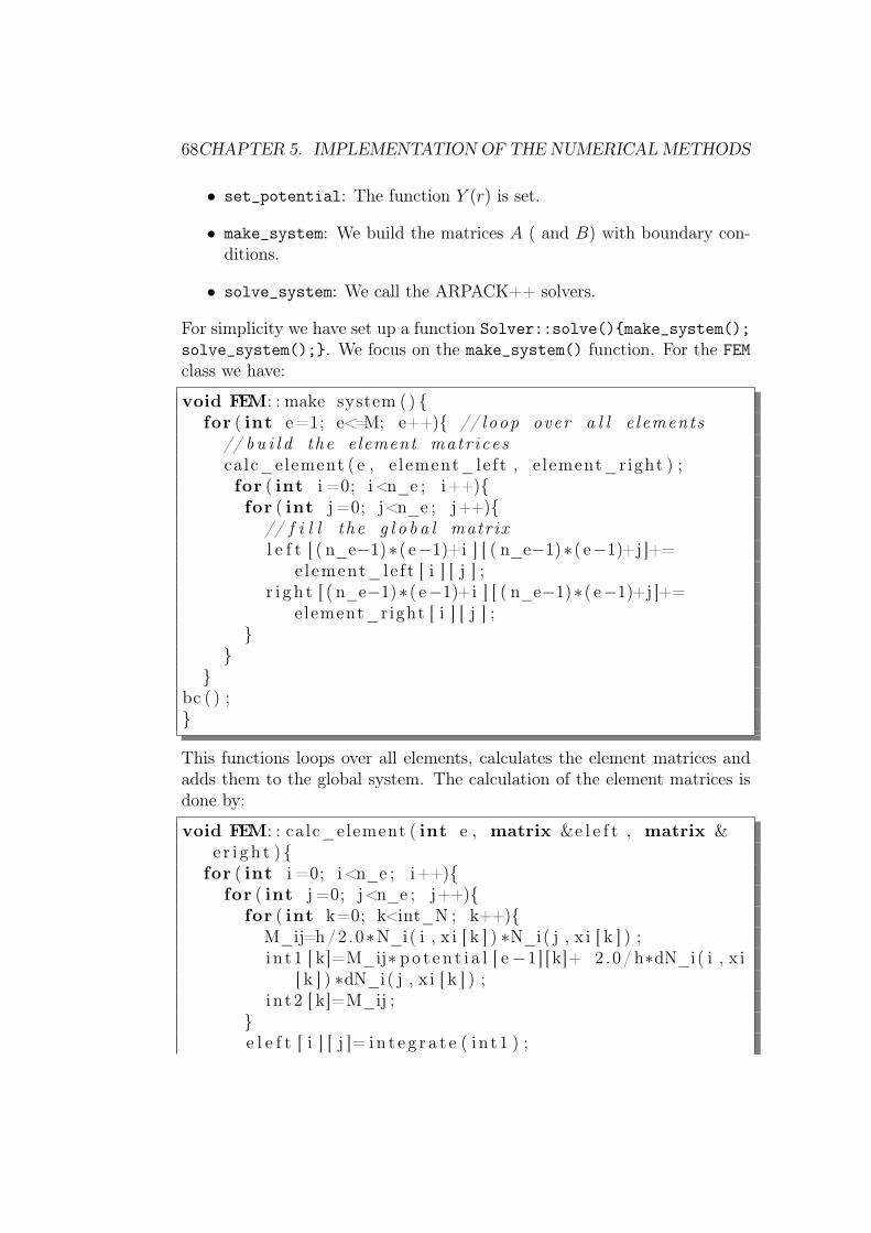
68CHAPTER 5. IMPLEMENTATION OF THE NUMERICAL METHODS
• set_potential: The function Y (r) is set.
• make_system: We build the matrices A ( and B) with boundary con-ditions.
• solve_system: We call the ARPACK++ solvers.
For simplicity we have set up a function Solver::solve()make_system();solve_system();. We focus on the make_system() function. For the FEMclass we have:
void FEM: : make system ( ) for ( int e=1; e<=M; e++) // loop over a l l e lements
// b u i l d the element matr icescalc_element ( e , e lement_le f t , e lement_right ) ;for ( int i =0; i<n_e ; i++)for ( int j =0; j<n_e ; j++)
// f i l l t he g l o b a l matrixl e f t [ ( n_e−1)∗( e−1)+i ] [ ( n_e−1)∗( e−1)+j ]+=
element_le f t [ i ] [ j ] ;r i g h t [ ( n_e−1)∗( e−1)+i ] [ ( n_e−1)∗( e−1)+j ]+=
element_right [ i ] [ j ] ;
bc ( ) ;
This functions loops over all elements, calculates the element matrices andadds them to the global system. The calculation of the element matrices isdone by:
void FEM: : ca lc_element ( int e , matrix &e l e f t , matrix &er i gh t )
for ( int i =0; i<n_e ; i++)for ( int j =0; j<n_e ; j++)
for ( int k=0; k<int_N ; k++)M_ij=h/2.0∗N_i( i , x i [ k ] ) ∗N_i( j , x i [ k ] ) ;i n t1 [ k]=M_ij∗ po t e n t i a l [ e−1] [ k]+ 2 .0/h∗dN_i( i , x i
[ k ] ) ∗dN_i( j , x i [ k ] ) ;i n t2 [ k]=M_ij ;
e l e f t [ i ] [ j ]= i n t e g r a t e ( i n t1 ) ;
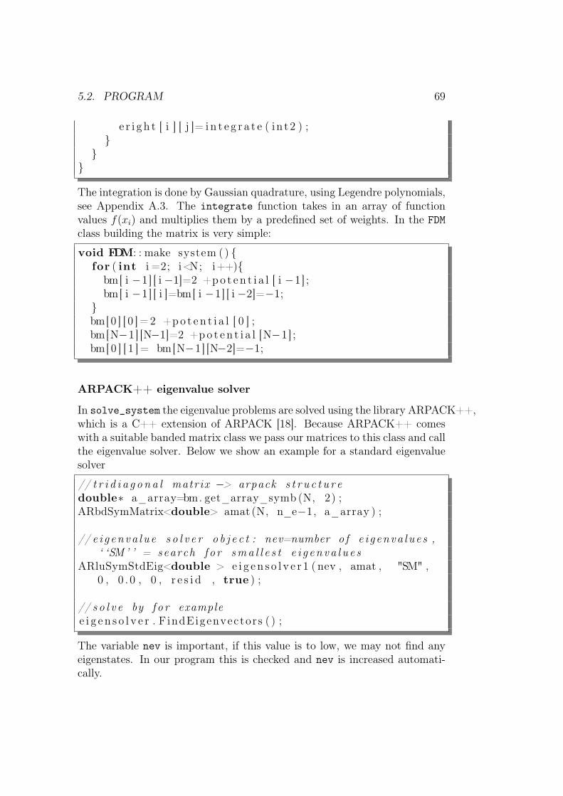
5.2. PROGRAM 69
e r i g h t [ i ] [ j ]= i n t e g r a t e ( i n t2 ) ;
The integration is done by Gaussian quadrature, using Legendre polynomials,see Appendix A.3. The integrate function takes in an array of functionvalues f(xi) and multiplies them by a predefined set of weights. In the FDMclass building the matrix is very simple:
void FDM: : make system ( ) for ( int i =2; i<N; i++)
bm[ i −1] [ i −1]=2 +po t en t i a l [ i −1] ;bm[ i −1] [ i ]=bm[ i −1] [ i −2]=−1;
bm[ 0 ] [ 0 ]=2 +po t en t i a l [ 0 ] ;bm[N−1] [N−1]=2 +po t en t i a l [N−1] ;bm[ 0 ] [ 1 ]= bm[N−1] [N−2]=−1;
ARPACK++ eigenvalue solver
In solve_system the eigenvalue problems are solved using the library ARPACK++,which is a C++ extension of ARPACK [18]. Because ARPACK++ comeswith a suitable banded matrix class we pass our matrices to this class and callthe eigenvalue solver. Below we show an example for a standard eigenvaluesolver
// t r i d i a g o n a l matrix −> arpack s t r u c t u r edouble∗ a_array=bm. get_array_symb (N, 2) ;ARbdSymMatrix<double> amat (N, n_e−1, a_array ) ;
// e i g enva l u e s o l v e r o b j e c t : nev=number o f e i g enva lue s ,‘ ‘SM ’ ’ = search f o r sma l l e s t e i g en va l u e s
ARluSymStdEig<double > e i g en s o l v e r 1 ( nev , amat , "SM" ,0 , 0 . 0 , 0 , r e s i d , true ) ;
// s o l v e by f o r examplee i g e n s o l v e r . F indEigenvectors ( ) ;
The variable nev is important, if this value is to low, we may not find anyeigenstates. In our program this is checked and nev is increased automati-cally.
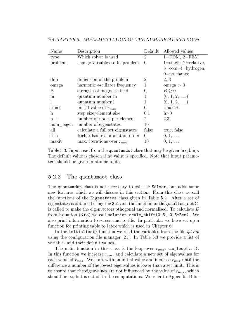
70CHAPTER 5. IMPLEMENTATION OF THE NUMERICAL METHODS
Name Description Default Allowed valuestype Which solver is used 2 1=FDM, 2=FEMproblem change variables to fit problem 0 1=single, 2=relative,
3=com, 4=hydrogen,0=no change
dim dimension of the problem 2 2, 3omega harmonic oscillator frequency 1 omega > 0B strength of magnetic field 0 B ≥ 0m quantum number m 1 (0, 1, 2, . . . )l quantum number l 1 (0, 1, 2, . . . )rmax initial value of rmax 0 rmax>0h step size/element size 0.1 h>0n_e number of nodes per element 2 2,3num_eigen number of eigenstates 10all calculate a full set eigenstates false true, falserich Richardson extrapolation order 0 0, 1, . . .maxit max. iterations over rmax 10 0, 1, . . .
Table 5.3: Input read from the quantumdot class that may be given in qd.inp.The default value is chosen if no value is specified. Note that input parame-ters should be given in atomic units.
5.2.2 The quantumdot class
The quantumdot class is not necessary to call the Solver, but adds somenew features which we will discuss in this section. From this class we callthe functions of the Eigenstates class given in Table 5.2. After a set ofeigenstates is obtained using the Solver, the function orthogonalise_set()is called to make the eigenvectors othogonal and normalised. To calculate Efrom Equation (3.63) we call solution.scale_shift(0.5, 0.5*B*m). Wealso print information to screen and to file. In particular we have set up afunction for printing table to latex which is used in Chapter 6.
In the initialise() function we read the variables from the file qd.inpusing the configuration file manager [21]. In Table 5.3 we provide a list ofvariables and their default values.
The main function in this class is the loop over rmax: rm_loop(...).In this function we increase rmax and calculate a new set of eigenvalues foreach value of rmax. We start with an initial value and increase rmax until thedifference a number of the lowest eigenvalues is lower than a set limit. This isto ensure that the eigenvalues are not influenced by the value of rmax, whichshould be ∞, but is cut off in the computations. We refer to Appendix B for
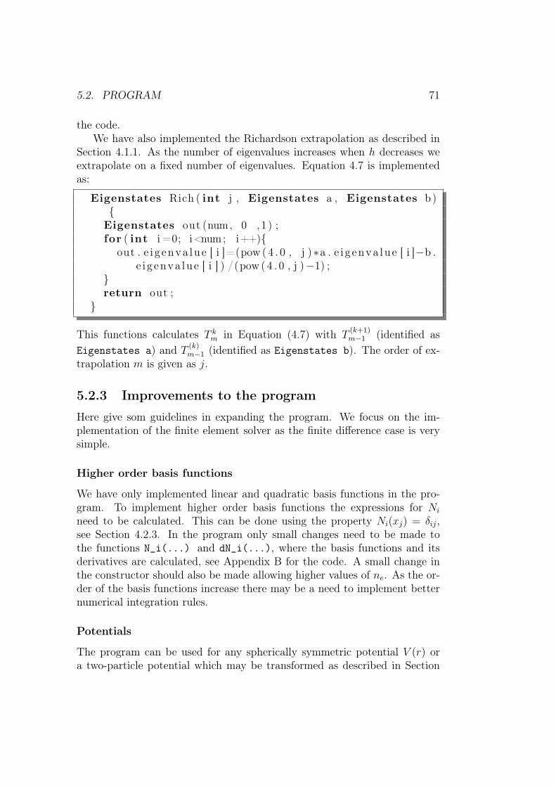
5.2. PROGRAM 71
the code.We have also implemented the Richardson extrapolation as described in
Section 4.1.1. As the number of eigenvalues increases when h decreases weextrapolate on a fixed number of eigenvalues. Equation 4.7 is implementedas:
Eigenstates Rich ( int j , Eigenstates a , Eigenstates b)
Eigenstates out (num, 0 ,1 ) ;for ( int i =0; i<num; i++)
out . e i g enva lue [ i ]=(pow ( 4 . 0 , j )∗a . e i g enva lue [ i ]−b .e i g enva lue [ i ] ) /(pow ( 4 . 0 , j )−1) ;
return out ;
This functions calculates T km in Equation (4.7) with T
(k+1)m−1 (identified as
Eigenstates a) and T(k)m−1 (identified as Eigenstates b). The order of ex-
trapolation m is given as j.
5.2.3 Improvements to the program
Here give som guidelines in expanding the program. We focus on the im-plementation of the finite element solver as the finite difference case is verysimple.
Higher order basis functions
We have only implemented linear and quadratic basis functions in the pro-gram. To implement higher order basis functions the expressions for Ni
need to be calculated. This can be done using the property Ni(xj) = δij,see Section 4.2.3. In the program only small changes need to be made tothe functions N_i(...) and dN_i(...), where the basis functions and itsderivatives are calculated, see Appendix B for the code. A small change inthe constructor should also be made allowing higher values of ne. As the or-der of the basis functions increase there may be a need to implement betternumerical integration rules.
Potentials
The program can be used for any spherically symmetric potential V (r) ora two-particle potential which may be transformed as described in Section
72CHAPTER 5. IMPLEMENTATION OF THE NUMERICAL METHODS
3.4: V (r1, r2) → V (r)+V (R). The program is set up to handle potentials ofthe form V (r) = Ar2 + B
r, but by changing the set_potential function this
potential may have another form. Note that this functionality must also beadded to the FDM class in the same way.
Uneven step length
We may choose to vary the size of the elements h → he. To implement thiswe need to calculate the node positions xq. An array of element sizes he mustalso be implemented. This improvement can be used to improve the accuracyclose to r = 0 where the wave functions change more rapidly. To implementthis the uneven step length must also be implemented in class Eigenstatesfor correct normalisation.
General time optimisation
The code could be more optimised in order to run faster, however the mosttime consuming part is the eigenvalue solver, which was not made as a partof this thesis.
Parallelisation
The parallelisation of a program like this is a complicated task, we must firstpartition the data and then use a parallel eigenvalue solver. For the parallelsolver we tried to use P_ARPACK [18], which seemed to be a good solver,however we were not able to install the library. For the first part we could usethe FEM and FDM class as they are implemented with a few changes. To usethe sequential code to build local matrices, we must first divide the elements(or nodes for the finite difference method), and set a local rmin value. ForP processors we can define the local number of elements m_i. If we have Mtotal element to divide among P processors we can divide the elements bythe code:
int m_i=M/P;int r e s t=M%P;i f (my_rank>0 && my_rank<=r e s t ) m_i++;
The value rmin must also be calculated, this can be dine by calculating rmax =h ∗mi on processor i and passing it to rmin on processor i+ 1. Then we callthe solvers as before to build local matrices. Changes must also be made tothe structure of class eigenstates, and we need to implement changes tothe linear algebra operations as explained in Section 4.3.
5.3. IMPLEMENTATION OF TIME EVOLUTION 73
5.3 Implementation of time evolutionThe Hamiltonian is split into a time-dependent part and a time-independentpart
H = H0 +H1(t). (5.24)
For H0 we calculate a full set of orthogonal eigenvectors u and correspondingeigenvalues E using the radial solver. Using these eigenfunctions we definean eigenvector basis as we explained in Section 4.4. We use the Blanes-Moanmethod, see Equations (4.60)-(4.65) in Section 4.4.
We have set up the time evolution in a matlab script. The script readsthe solutions for H0 from file and sets up the eigenvector matrix P and adiagonal matrix E of the eigenvalues. The step length ∆t and total time Tmust be given.
We must also set an initial state d(0) = P Tc(0) given in the eigenvectorbasis. Here c is the state vector in coordinate basis and d is the state vectorin the eigenvector basis. The time-independent Hamiltonian H0 gives thediagonal matrix E in the eigenvector basis.
We use the function H1(t) = W sin(ft) as the time-dependent perturba-tion and calculate the integrals analytically for now. The constants f andW must also be given, if W = 0 there is no time perturbation and we cancompare to analytic results. The analytic expressions for the integrals are∫
sin(ft)dt = − 1
fcos(ft), (5.25)∫
t sin(ft)dt =1
f 2[sin(ft)− tf cos(ft)] . (5.26)
For a spatially independent H1(t), H(k) is just the identity matrix times ascalar which is calculated from the integrals above. If H1(t) also depends onr we must transform it in the same basis, and we get a matrix.
For each time step we calculate c(t+∆t) = U(t+∆t, t)c(t) using Equation(4.60). To calculate the expression w = eMu, where M is a matrix, we usethe function expv from Expokit [22] in matlab.

Chapter 6
Results of numerical simulations
We begin by studying the single-electron quantum dot in two and threedimensions. We compare the results to known analytic results, in order toverify our solver. Then we move to the relative coordinates equation of thetwo-electron case and study the special analytic solutions from References[10] and [11].
6.1 Single electron quantum dot
In Chapter 3 we simplified the single particle equation to
2D: − d2u
dr2+
[m2 − 1
4
r2+ Ω2r2+
]u = εu, (6.1)
3D: − d2u
dr2+
[l(l + 1)
r2+ Ω2r2+
]u = εu. (6.2)
This is the equation for both the single particle equation and the centre-of-mass equation for the two-particle problem (when the constants are scaledas in Equation (3.66)). However the scaling is not important for the nu-merical algorithm. The analytic solutions are given in Section 3.3. In twodimemensions they are
ε
2Ω= (|m|+ 1 + 2n), (6.3)
u(r) =
√n!
π(m+ n)!ω(|m|+1)/2r|m|+ 1
2 e−12Ωr2
L|m|n (Ωr2). (6.4)
75
76 CHAPTER 6. RESULTS OF NUMERICAL SIMULATIONS
In three dimensions the solutions areε
2Ω= (2n+ l +
3
2), (6.5)
u(r) =
√2n+l+2n!√
π(2n+ 2l + 1)!!ω(l+3/2)/2rl+1e−ωr2/2L
l+ 12
n (ωr2). (6.6)
For the simulations we only use positive values for m because Equation (6.1)is only dependent on |m|. First we study the dependency on the variablermax.
6.1.1 Dependence on rmax
The solution domain for Equation (6.1) is r ∈ (0,∞). In the numericallysimulation we have to cut off this domain to r ∈ (0, rmax). We wish to set thiscut-off to a value which will not influence our results. For a chosen numberof wanted eigenvalues we increase the value of rmax until the difference inthis set of eigenvalues is small.
We set the variables: (m = 1, Ω = 1, h = 0.05) and run simulationsfor both the finite difference method and for the finite element method usinglinear elements. We vary the number of eigenvalues we request.. The value ofrmax which was found is given in Table 6.1. From this table we observe thatwhen we increase the number of required eigenvalues, we must also increasermax. In Figure 6.1 a plot of the wave functions are given, from this we seethat the higher energy wave functions stretch further out towards rmax. Thetwo methods give approximately the same results for rmax.
We also do a comparison between two values of rmax where we search forall the eigenvalues in the set. The results are given in Table 6.3 and 6.4.We observe that the lowest eigenvalues are the same for both sets, while forhigher eigenvalues the results depend on the value of rmax. When we increasermax we also increase the size of the system N = rmax
h+1. Because of this we
will never be able to find accurate values for all N eigenvalues, but we canchoose the number of accurate eigenvalues we need.
For the oscillator frequency Ω we do a similar examination of rmax. Theresults are given in Table 6.2. From the analytic wave functions in Equation(6.4) we see that the term e−
12Ωr2 will make the wave functions stretch further
out for lower values of Ω. Another way to explain this is to look directlyEquation (6.1). For the single-electron quantum dot we can introduce a newscaling r′ =
√Ωr. Using a scaling like this we should be able to solve one
equation and scale the result to fit for and Ω. From this formula rmax shouldbehave as we see in Table 6.2; When Ω decreases, we must increase rmax andthen r′max =
√Ωrmax stays the same. The variable h, ne do not affect rmax.
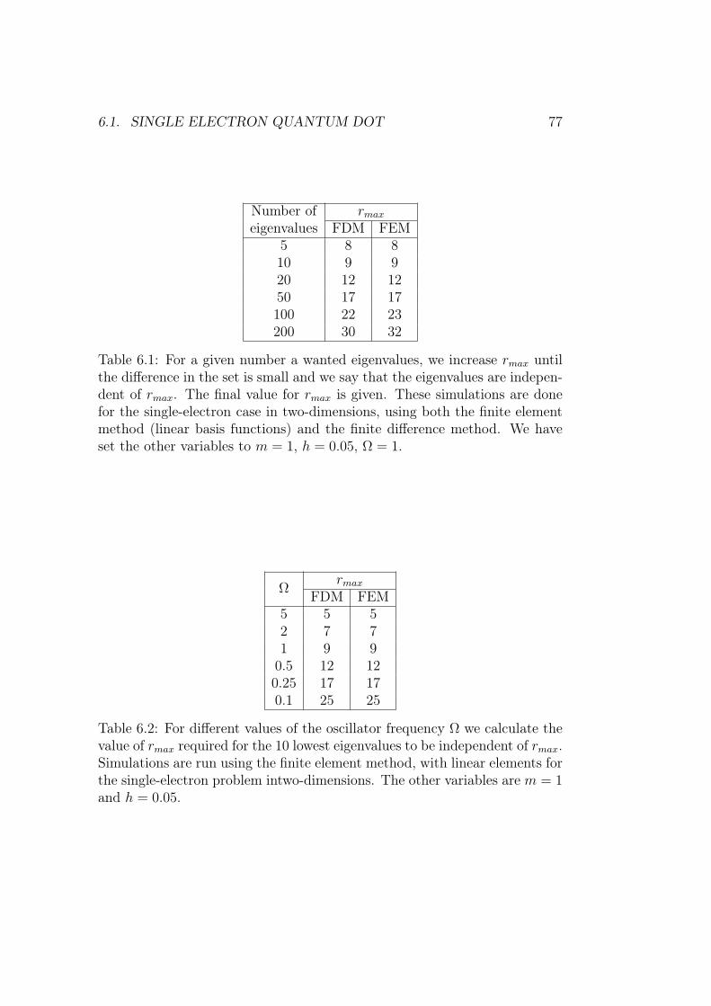
6.1. SINGLE ELECTRON QUANTUM DOT 77
Number of rmax
eigenvalues FDM FEM5 8 810 9 920 12 1250 17 17100 22 23200 30 32
Table 6.1: For a given number a wanted eigenvalues, we increase rmax untilthe difference in the set is small and we say that the eigenvalues are indepen-dent of rmax. The final value for rmax is given. These simulations are donefor the single-electron case in two-dimensions, using both the finite elementmethod (linear basis functions) and the finite difference method. We haveset the other variables to m = 1, h = 0.05, Ω = 1.
Ωrmax
FDM FEM5 5 52 7 71 9 9
0.5 12 120.25 17 170.1 25 25
Table 6.2: For different values of the oscillator frequency Ω we calculate thevalue of rmax required for the 10 lowest eigenvalues to be independent of rmax.Simulations are run using the finite element method, with linear elements forthe single-electron problem intwo-dimensions. The other variables are m = 1and h = 0.05.
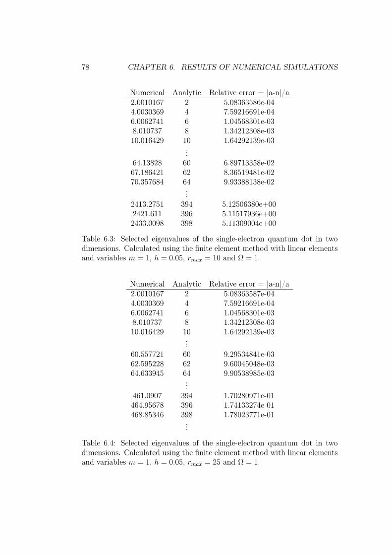
78 CHAPTER 6. RESULTS OF NUMERICAL SIMULATIONS
Numerical Analytic Relative error = |a-n|/a2.0010167 2 5.08363586e-044.0030369 4 7.59216691e-046.0062741 6 1.04568301e-038.010737 8 1.34212308e-0310.016429 10 1.64292139e-03
...64.13828 60 6.89713358e-0267.186421 62 8.36519481e-0270.357684 64 9.93388138e-02
...2413.2751 394 5.12506380e+002421.611 396 5.11517936e+002433.0098 398 5.11309004e+00
Table 6.3: Selected eigenvalues of the single-electron quantum dot in twodimensions. Calculated using the finite element method with linear elementsand variables m = 1, h = 0.05, rmax = 10 and Ω = 1.
Numerical Analytic Relative error = |a-n|/a2.0010167 2 5.08363587e-044.0030369 4 7.59216691e-046.0062741 6 1.04568301e-038.010737 8 1.34212308e-0310.016429 10 1.64292139e-03
...60.557721 60 9.29534841e-0362.595228 62 9.60045048e-0364.633945 64 9.90538985e-03
...461.0907 394 1.70280971e-01464.95678 396 1.74133274e-01468.85346 398 1.78023771e-01
...
Table 6.4: Selected eigenvalues of the single-electron quantum dot in twodimensions. Calculated using the finite element method with linear elementsand variables m = 1, h = 0.05, rmax = 25 and Ω = 1.
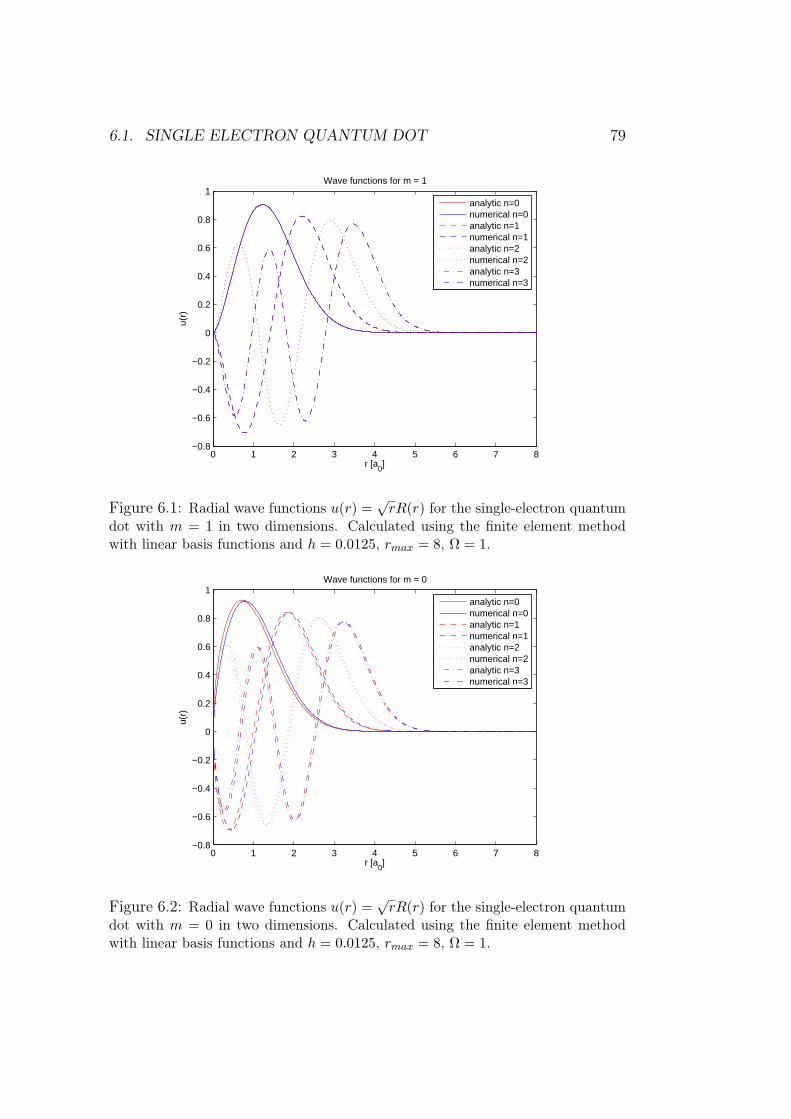
6.1. SINGLE ELECTRON QUANTUM DOT 79
0 1 2 3 4 5 6 7 8−0.8
−0.6
−0.4
−0.2
0
0.2
0.4
0.6
0.8
1Wave functions for m = 1
r [a0]
u(r)
analytic n=0numerical n=0analytic n=1numerical n=1analytic n=2numerical n=2analytic n=3numerical n=3
Figure 6.1: Radial wave functions u(r) =√
rR(r) for the single-electron quantumdot with m = 1 in two dimensions. Calculated using the finite element methodwith linear basis functions and h = 0.0125, rmax = 8, Ω = 1.
0 1 2 3 4 5 6 7 8−0.8
−0.6
−0.4
−0.2
0
0.2
0.4
0.6
0.8
1Wave functions for m = 0
r [a0]
u(r)
analytic n=0numerical n=0analytic n=1numerical n=1analytic n=2numerical n=2analytic n=3numerical n=3
Figure 6.2: Radial wave functions u(r) =√
rR(r) for the single-electron quantumdot with m = 0 in two dimensions. Calculated using the finite element methodwith linear basis functions and h = 0.0125, rmax = 8, Ω = 1.
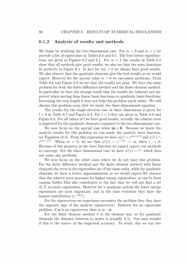
80 CHAPTER 6. RESULTS OF NUMERICAL SIMULATIONS
6.1.2 Analysis of results and methods
We begin by studying the two-dimensional case. For m = 0 and m = 1 weprovide a list of eigenvalues in Tables 6.6 and 6.5. The four lowest eigenfunc-tions are given in Figures 6.2 and 6.1. For m = 1 the results in Table 6.5show that all methods give good results, we also see that the wave functionsfit perfectly in Figure 6.1. In fact for |m| > 0 we always have good results.We also observe that the quadratic elements give the best results as we wouldexpect. However for the special value m = 0 we encounter problems. FromTable 6.6 and Figure 6.2 we see that the results are poor. We have the sameproblem for both the finite difference method and the finite element method.In particular we have the strange result that the results are (almost) not im-proved when moving from linear basis functions to quadratic basis functions.Increasing the step length h does not help this problem much either. We willdiscuss this problem soon, first we study the three-dimensional equation.
The results for the single-electron case in three dimensions is given forl = 0 in Table 6.7 and Figure 6.3. For l = 5 they are given in Table 6.8 andFigure 6.4. For all values of l we have good results, actually the relative erroris improved for the quadratic elements compared to the two-dimensional case.
We now focus on the special case when m = 0. Because we know theanalytic results for this problem we can study the analytic wave function,see Equation (6.4). From this expression we have u(r) ∼ r|m|+1/2 and u′(r) ∼r|m|−1/2. When m = 0, we see that u′(r) ∼ r−1/2 → ∞ when r → 0.Because of this property in the wave function we cannot expect our methodsto converge. For the three dimensional case we have u′(r) ∼ rl, which doesnot cause any problems.
We now focus on the other cases where we do not have this problem.For the finite difference method and the finite element method with linearelements the error in the eigenvalues are of the same order, while for quadraticelements we have a better approximations as we would expect.We observethat the relative error increases for higher energy eigenvalues, as can be fromvarious Tables.This also contributes to the fact that we will not find a setof N accurate eigenvalues. However for a quantum system the lower energyeigenstates are most important, and in the time evolution they have thelargest contribution (e−iEkt).
For the eigenvectors we sometimes encounter the problem they they havethe opposite sign of the analytic eigenvectors. However for an eigenvalueproblem, if u is an eigenvector then so is −u.
For the finite element method h is the element size, so for quadraticelements the distance between to nodes is actually h/2. You may wonderif this is the source of the improved accuracy. To study this we run two
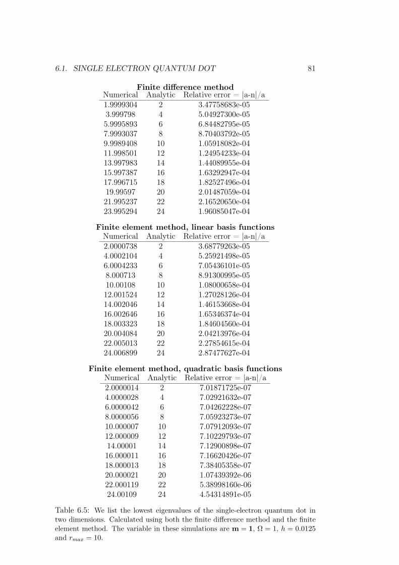
6.1. SINGLE ELECTRON QUANTUM DOT 81
Finite difference methodNumerical Analytic Relative error = |a-n|/a1.9999304 2 3.47758683e-053.999798 4 5.04927300e-055.9995893 6 6.84482795e-057.9993037 8 8.70403792e-059.9989408 10 1.05918082e-0411.998501 12 1.24954233e-0413.997983 14 1.44089955e-0415.997387 16 1.63292947e-0417.996715 18 1.82527496e-0419.99597 20 2.01487059e-0421.995237 22 2.16520650e-0423.995294 24 1.96085047e-04
Finite element method, linear basis functionsNumerical Analytic Relative error = |a-n|/a2.0000738 2 3.68779263e-054.0002104 4 5.25921498e-056.0004233 6 7.05436101e-058.000713 8 8.91300995e-0510.00108 10 1.08000658e-0412.001524 12 1.27028126e-0414.002046 14 1.46153668e-0416.002646 16 1.65346374e-0418.003323 18 1.84604560e-0420.004084 20 2.04213976e-0422.005013 22 2.27854615e-0424.006899 24 2.87477627e-04
Finite element method, quadratic basis functionsNumerical Analytic Relative error = |a-n|/a2.0000014 2 7.01871725e-074.0000028 4 7.02921632e-076.0000042 6 7.04262228e-078.0000056 8 7.05923273e-0710.000007 10 7.07912093e-0712.000009 12 7.10229793e-0714.00001 14 7.12900898e-0716.000011 16 7.16620426e-0718.000013 18 7.38405358e-0720.000021 20 1.07439392e-0622.000119 22 5.38998160e-0624.00109 24 4.54314891e-05
Table 6.5: We list the lowest eigenvalues of the single-electron quantum dot intwo dimensions. Calculated using both the finite difference method and the finiteelement method. The variable in these simulations are m = 1, Ω = 1, h = 0.0125and rmax = 10.
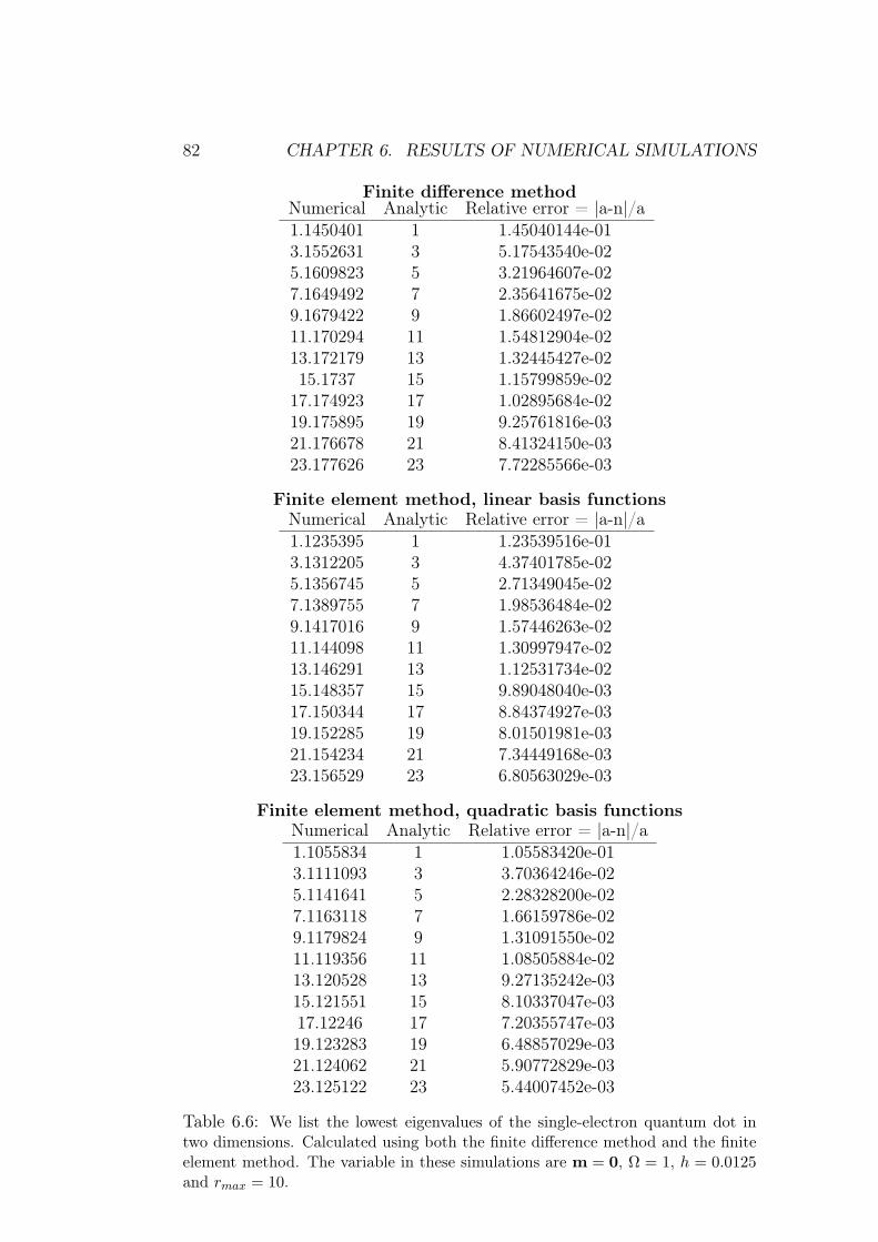
82 CHAPTER 6. RESULTS OF NUMERICAL SIMULATIONS
Finite difference methodNumerical Analytic Relative error = |a-n|/a1.1450401 1 1.45040144e-013.1552631 3 5.17543540e-025.1609823 5 3.21964607e-027.1649492 7 2.35641675e-029.1679422 9 1.86602497e-0211.170294 11 1.54812904e-0213.172179 13 1.32445427e-0215.1737 15 1.15799859e-02
17.174923 17 1.02895684e-0219.175895 19 9.25761816e-0321.176678 21 8.41324150e-0323.177626 23 7.72285566e-03
Finite element method, linear basis functionsNumerical Analytic Relative error = |a-n|/a1.1235395 1 1.23539516e-013.1312205 3 4.37401785e-025.1356745 5 2.71349045e-027.1389755 7 1.98536484e-029.1417016 9 1.57446263e-0211.144098 11 1.30997947e-0213.146291 13 1.12531734e-0215.148357 15 9.89048040e-0317.150344 17 8.84374927e-0319.152285 19 8.01501981e-0321.154234 21 7.34449168e-0323.156529 23 6.80563029e-03
Finite element method, quadratic basis functionsNumerical Analytic Relative error = |a-n|/a1.1055834 1 1.05583420e-013.1111093 3 3.70364246e-025.1141641 5 2.28328200e-027.1163118 7 1.66159786e-029.1179824 9 1.31091550e-0211.119356 11 1.08505884e-0213.120528 13 9.27135242e-0315.121551 15 8.10337047e-0317.12246 17 7.20355747e-0319.123283 19 6.48857029e-0321.124062 21 5.90772829e-0323.125122 23 5.44007452e-03
Table 6.6: We list the lowest eigenvalues of the single-electron quantum dot intwo dimensions. Calculated using both the finite difference method and the finiteelement method. The variable in these simulations are m = 0, Ω = 1, h = 0.0125and rmax = 10.
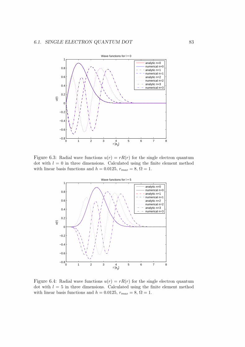
6.1. SINGLE ELECTRON QUANTUM DOT 83
0 1 2 3 4 5 6 7 8−0.8
−0.6
−0.4
−0.2
0
0.2
0.4
0.6
0.8
1Wave functions for l = 0
r [a0]
u(r)
analytic n=0numerical n=0analytic n=1numerical n=1analytic n=2numerical n=2analytic n=3numerical n=3
Figure 6.3: Radial wave functions u(r) = rR(r) for the single electron quantumdot with l = 0 in three dimensions. Calculated using the finite element methodwith linear basis functions and h = 0.0125, rmax = 8, Ω = 1.
0 1 2 3 4 5 6 7 8−0.8
−0.6
−0.4
−0.2
0
0.2
0.4
0.6
0.8
1Wave functions for l = 5
r [a0]
u(r)
analytic n=0numerical n=0analytic n=1numerical n=1analytic n=2numerical n=2analytic n=3numerical n=3
Figure 6.4: Radial wave functions u(r) = rR(r) for the single electron quantumdot with l = 5 in three dimensions. Calculated using the finite element methodwith linear basis functions and h = 0.0125, rmax = 8, Ω = 1.
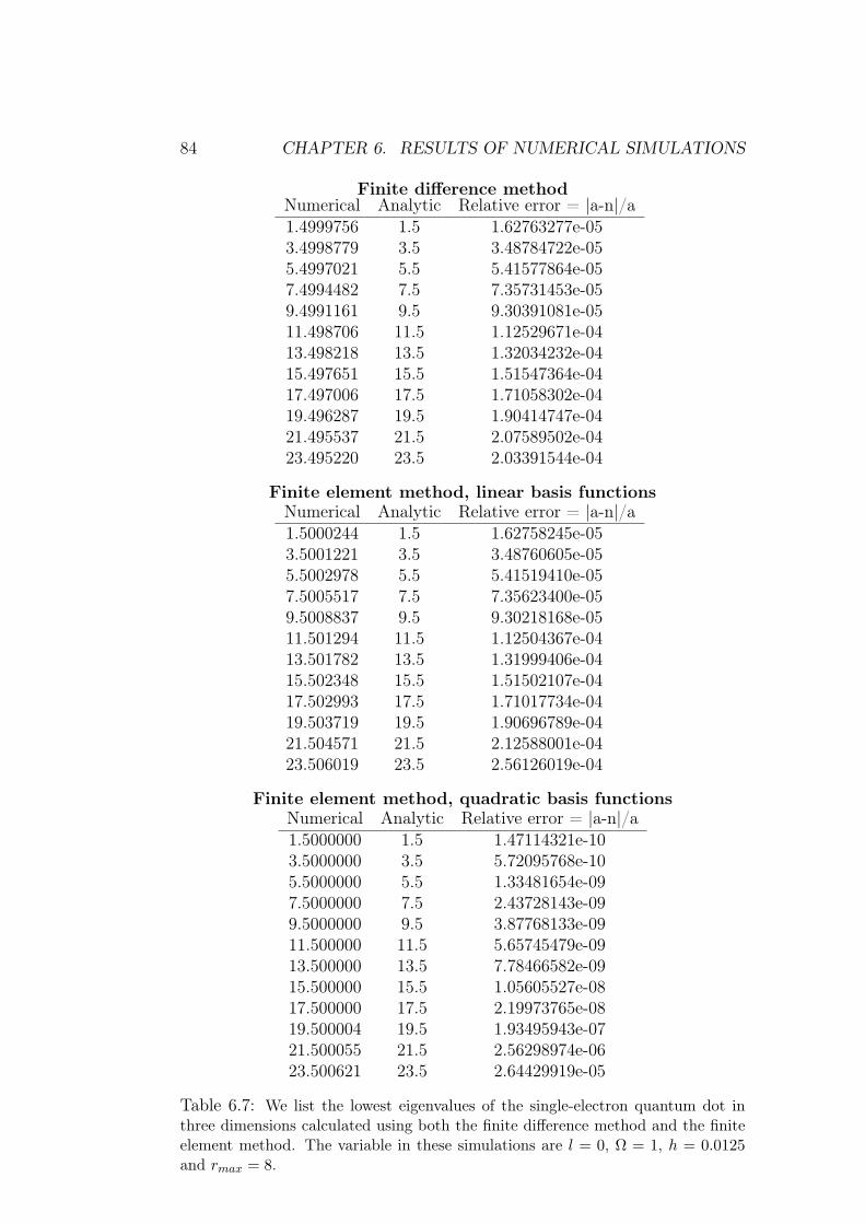
84 CHAPTER 6. RESULTS OF NUMERICAL SIMULATIONS
Finite difference methodNumerical Analytic Relative error = |a-n|/a1.4999756 1.5 1.62763277e-053.4998779 3.5 3.48784722e-055.4997021 5.5 5.41577864e-057.4994482 7.5 7.35731453e-059.4991161 9.5 9.30391081e-0511.498706 11.5 1.12529671e-0413.498218 13.5 1.32034232e-0415.497651 15.5 1.51547364e-0417.497006 17.5 1.71058302e-0419.496287 19.5 1.90414747e-0421.495537 21.5 2.07589502e-0423.495220 23.5 2.03391544e-04
Finite element method, linear basis functionsNumerical Analytic Relative error = |a-n|/a1.5000244 1.5 1.62758245e-053.5001221 3.5 3.48760605e-055.5002978 5.5 5.41519410e-057.5005517 7.5 7.35623400e-059.5008837 9.5 9.30218168e-0511.501294 11.5 1.12504367e-0413.501782 13.5 1.31999406e-0415.502348 15.5 1.51502107e-0417.502993 17.5 1.71017734e-0419.503719 19.5 1.90696789e-0421.504571 21.5 2.12588001e-0423.506019 23.5 2.56126019e-04
Finite element method, quadratic basis functionsNumerical Analytic Relative error = |a-n|/a1.5000000 1.5 1.47114321e-103.5000000 3.5 5.72095768e-105.5000000 5.5 1.33481654e-097.5000000 7.5 2.43728143e-099.5000000 9.5 3.87768133e-0911.500000 11.5 5.65745479e-0913.500000 13.5 7.78466582e-0915.500000 15.5 1.05605527e-0817.500000 17.5 2.19973765e-0819.500004 19.5 1.93495943e-0721.500055 21.5 2.56298974e-0623.500621 23.5 2.64429919e-05
Table 6.7: We list the lowest eigenvalues of the single-electron quantum dot inthree dimensions calculated using both the finite difference method and the finiteelement method. The variable in these simulations are l = 0, Ω = 1, h = 0.0125and rmax = 8.

6.1. SINGLE ELECTRON QUANTUM DOT 85
Finite difference methodNumerical Analytic Relative error = |a-n|/a6.4999785 6.5 3.30079248e-068.4998968 8.5 1.21388049e-0510.499737 10.5 2.50510850e-0512.499499 12.5 4.00823503e-0514.499183 14.5 5.63560713e-0516.498789 16.5 7.34198565e-0518.498317 18.5 9.09959390e-0520.497775 20.5 1.08551731e-0422.497269 22.5 1.21364539e-0424.497791 24.5 9.01533094e-0526.505445 26.5 2.05464543e-0428.543458 28.5 1.52484023e-03
Finite element method, linear basis functionsNumerical Analytic Relative error = |a-n|/a6.5000215 6.5 3.30074116e-068.5001032 8.5 1.21381462e-0510.500263 10.5 2.50487599e-0512.500501 12.5 4.00770768e-0514.500817 14.5 5.63465136e-0516.501211 16.5 7.34063445e-0518.501684 18.5 9.10218285e-0520.502243 20.5 1.09415055e-0422.502996 22.5 1.33140178e-0424.504941 24.5 2.01666020e-0426.514235 26.5 5.37184126e-0428.554294 28.5 1.90506711e-03
Finite element method, quadratic basis functionsNumerical Analytic Relative error = |a-n|/a6.5000000 6.5 4.62243577e-118.5000000 8.5 2.31825435e-1010.500000 10.5 6.51294130e-1012.500000 12.5 1.35557300e-0914.500000 14.5 2.39091677e-0916.500000 16.5 4.62762725e-0918.500001 18.5 2.95981328e-0820.500009 20.5 4.54655861e-0722.500133 22.5 5.91820972e-0624.501367 24.5 5.57949383e-0526.509841 26.5 3.71370387e-0428.548878 28.5 1.71500277e-03
Table 6.8: We list the lowest eigenvalues of the single-electron quantum dot inthree dimensions calculated using both the finite difference method and the finiteelement method. The variable in these simulations are l = 5, Ω = 1, h = 0.0125and rmax = 8.
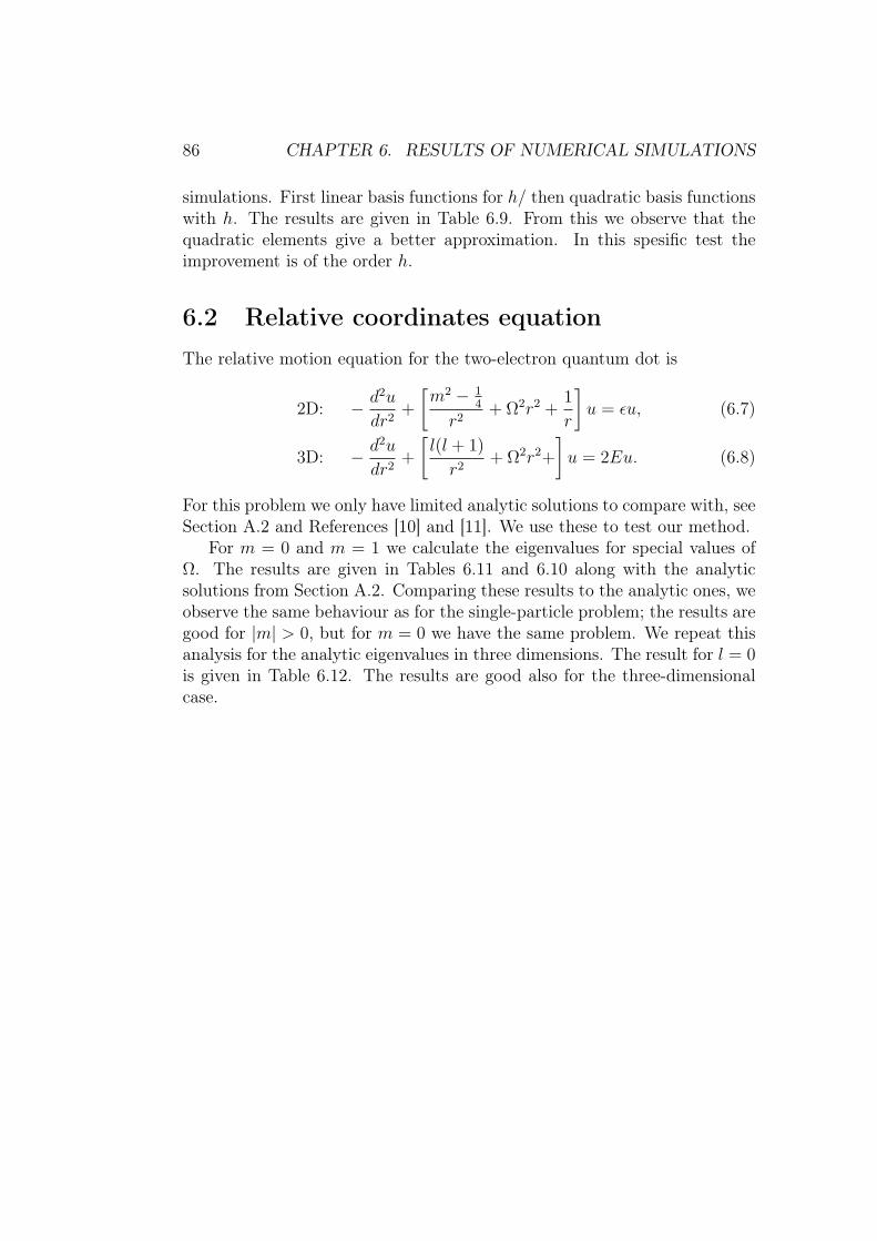
86 CHAPTER 6. RESULTS OF NUMERICAL SIMULATIONS
simulations. First linear basis functions for h/ then quadratic basis functionswith h. The results are given in Table 6.9. From this we observe that thequadratic elements give a better approximation. In this spesific test theimprovement is of the order h.
6.2 Relative coordinates equationThe relative motion equation for the two-electron quantum dot is
2D: − d2u
dr2+
[m2 − 1
4
r2+ Ω2r2 +
1
r
]u = εu, (6.7)
3D: − d2u
dr2+
[l(l + 1)
r2+ Ω2r2+
]u = 2Eu. (6.8)
For this problem we only have limited analytic solutions to compare with, seeSection A.2 and References [10] and [11]. We use these to test our method.
For m = 0 and m = 1 we calculate the eigenvalues for special values ofΩ. The results are given in Tables 6.11 and 6.10 along with the analyticsolutions from Section A.2. Comparing these results to the analytic ones, weobserve the same behaviour as for the single-particle problem; the results aregood for |m| > 0, but for m = 0 we have the same problem. We repeat thisanalysis for the analytic eigenvalues in three dimensions. The result for l = 0is given in Table 6.12. The results are good also for the three-dimensionalcase.
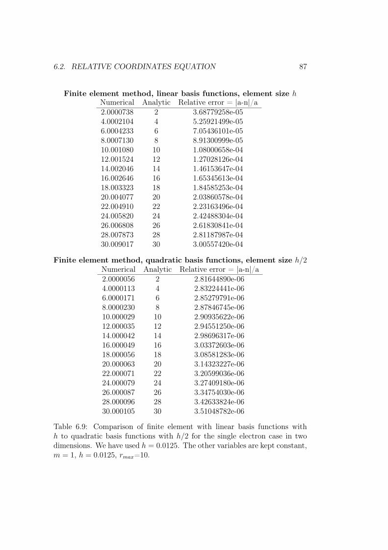
6.2. RELATIVE COORDINATES EQUATION 87
Finite element method, linear basis functions, element size hNumerical Analytic Relative error = |a-n|/a2.0000738 2 3.68779258e-054.0002104 4 5.25921499e-056.0004233 6 7.05436101e-058.0007130 8 8.91300999e-0510.001080 10 1.08000658e-0412.001524 12 1.27028126e-0414.002046 14 1.46153647e-0416.002646 16 1.65345613e-0418.003323 18 1.84585253e-0420.004077 20 2.03860578e-0422.004910 22 2.23163496e-0424.005820 24 2.42488304e-0426.006808 26 2.61830841e-0428.007873 28 2.81187987e-0430.009017 30 3.00557420e-04
Finite element method, quadratic basis functions, element size h/2Numerical Analytic Relative error = |a-n|/a2.0000056 2 2.81644890e-064.0000113 4 2.83224441e-066.0000171 6 2.85279791e-068.0000230 8 2.87846745e-0610.000029 10 2.90935622e-0612.000035 12 2.94551250e-0614.000042 14 2.98696317e-0616.000049 16 3.03372603e-0618.000056 18 3.08581283e-0620.000063 20 3.14323227e-0622.000071 22 3.20599036e-0624.000079 24 3.27409180e-0626.000087 26 3.34754030e-0628.000096 28 3.42633824e-0630.000105 30 3.51048782e-06
Table 6.9: Comparison of finite element with linear basis functions withh to quadratic basis functions with h/2 for the single electron case in twodimensions. We have used h = 0.0125. The other variables are kept constant,m = 1, h = 0.0125, rmax=10.
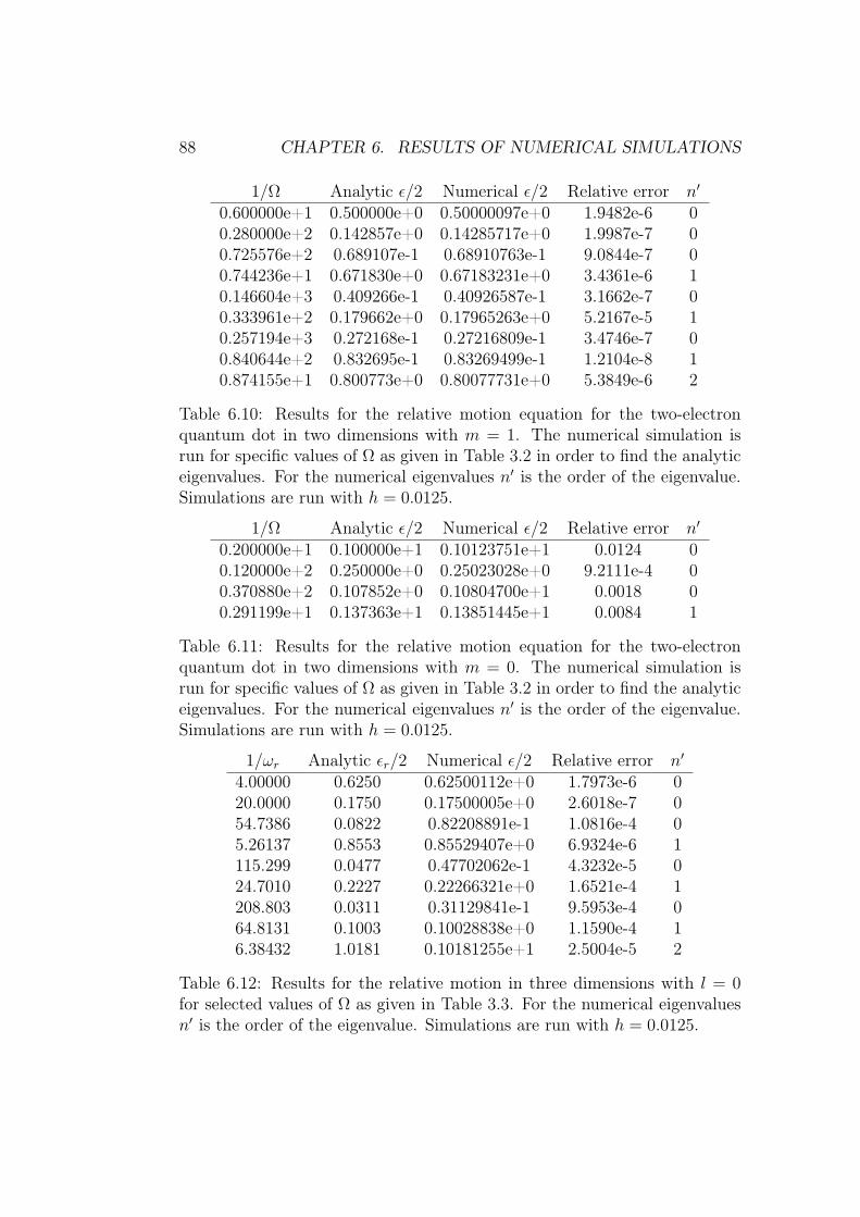
88 CHAPTER 6. RESULTS OF NUMERICAL SIMULATIONS
1/Ω Analytic ε/2 Numerical ε/2 Relative error n′
0.600000e+1 0.500000e+0 0.50000097e+0 1.9482e-6 00.280000e+2 0.142857e+0 0.14285717e+0 1.9987e-7 00.725576e+2 0.689107e-1 0.68910763e-1 9.0844e-7 00.744236e+1 0.671830e+0 0.67183231e+0 3.4361e-6 10.146604e+3 0.409266e-1 0.40926587e-1 3.1662e-7 00.333961e+2 0.179662e+0 0.17965263e+0 5.2167e-5 10.257194e+3 0.272168e-1 0.27216809e-1 3.4746e-7 00.840644e+2 0.832695e-1 0.83269499e-1 1.2104e-8 10.874155e+1 0.800773e+0 0.80077731e+0 5.3849e-6 2
Table 6.10: Results for the relative motion equation for the two-electronquantum dot in two dimensions with m = 1. The numerical simulation isrun for specific values of Ω as given in Table 3.2 in order to find the analyticeigenvalues. For the numerical eigenvalues n′ is the order of the eigenvalue.Simulations are run with h = 0.0125.
1/Ω Analytic ε/2 Numerical ε/2 Relative error n′
0.200000e+1 0.100000e+1 0.10123751e+1 0.0124 00.120000e+2 0.250000e+0 0.25023028e+0 9.2111e-4 00.370880e+2 0.107852e+0 0.10804700e+1 0.0018 00.291199e+1 0.137363e+1 0.13851445e+1 0.0084 1
Table 6.11: Results for the relative motion equation for the two-electronquantum dot in two dimensions with m = 0. The numerical simulation isrun for specific values of Ω as given in Table 3.2 in order to find the analyticeigenvalues. For the numerical eigenvalues n′ is the order of the eigenvalue.Simulations are run with h = 0.0125.
1/ωr Analytic εr/2 Numerical ε/2 Relative error n′
4.00000 0.6250 0.62500112e+0 1.7973e-6 020.0000 0.1750 0.17500005e+0 2.6018e-7 054.7386 0.0822 0.82208891e-1 1.0816e-4 05.26137 0.8553 0.85529407e+0 6.9324e-6 1115.299 0.0477 0.47702062e-1 4.3232e-5 024.7010 0.2227 0.22266321e+0 1.6521e-4 1208.803 0.0311 0.31129841e-1 9.5953e-4 064.8131 0.1003 0.10028838e+0 1.1590e-4 16.38432 1.0181 0.10181255e+1 2.5004e-5 2
Table 6.12: Results for the relative motion in three dimensions with l = 0for selected values of Ω as given in Table 3.3. For the numerical eigenvaluesn′ is the order of the eigenvalue. Simulations are run with h = 0.0125.
Chapter 7
Concluding remarks
The study in this thesis has been two-fold; it has been a study of the inter-esting quantum system of two-electrons in a quantum dot, but also a studyof the finite element method for solving the time-independent Schrödingerequation.
After giving a background to quantum mechanics we gave an overview ofquantum dots, focusing on the mathematical model. Note that this model isjust an approximation to a quantum dot. We showed that the one-electronquantum dot can be described by a modified harmonic oscillator, which is aknown quantum mechanical problem with analytic solutions. For the two-electron quantum dot we introduced centre-of-mass and relative motion co-ordinates and showed that the two-particle equation can be rewritten as twoindependent single particle equations. The centre-of-mass equation is also amodified harmonic oscillator equation, while the relative coordinates equa-tion is more complicated.
The other main topic of this thesis was the use of numerical methodsfor solving differential equations. We gave a thorough introduction to thefinite element method in one dimension and also mentioned the finite differ-ence method. Both methods were implemented in a program for solving thetime-independent Schrödinger equation for a spherically symmetric poten-tial. This program were then used to study the one-electron and two-electronquantum dot. We would have liked to parallelise this program as well, how-ever we had big problems making the P_ARPACK [18] library work.
After studying the results in Chapter 6 we see that our program give goodresults except for the special case when m = 0 in two dimensions where wediscovered that we have a divergence u′(r) ∼ r−1/2 → ∞. Compared to thefinite difference method the finite element method give results with approx-imately the same relative error for linear elements, however for quadratic
89
90 CHAPTER 7. CONCLUDING REMARKS
elements we get a better approximation. It is possible to extend the programwith higher order basis functions, see Section 5.2.3. A disadvantage of the fi-nite element method is that we end up with a generalised eigenvalue probleminstead of a standard eigenvalue problem. Fortunately the arpack++ libraryhas implemented this. However this may be more time consuming to solve,but this has not been studied in this thesis.
A very interesting problem is the double quantum dot, consisting of twocoupled quantum dots. This system is similar to the potential we have stud-ied. Unfortunately for us this problem breaks the spherical symmetry andcan not be studied by our model. To study this a two-dimensional (or three-dimensional) solver must be constructed.
Appendix A
Mathematical details
A.1 Analytic solutions of the single-electron har-monic oscillator
Here we derive the analytic solutions for the two-dimensional harmonic os-cillator. We begin with Equation (3.27) from Chapter 3
−[1
r
d
dr
(rd
dr
)− m2
r2
]R(r) +
(ω2r2 − ε
)R(r) = 0. (A.1)
First we study the limits r → 0 and r → ∞. For r → 0 the m2/r2 termdominates and we have
−[1
r
d
dr
(rd
dr
)− m2
r2
]R(r) = 0,
which has the solutionR(r) = r|m|.
For r →∞ the r2 term dominates
−[1
r
d
dr
(rd
dr
)]R(r) + ω2r2R(r) = 0,
and we have the solutionR(r) = e−
12ωr2/2.
Now we insert a solution of the form
R(r) = r|m|e−12ωr2
g(r), (A.2)
91
92 APPENDIX A. MATHEMATICAL DETAILS
into (A.1) to get
−d2g
dr2−
(2|m| − 2ωr2 + 1
) 1
r
dg
dr+ 2ω (|m|+ 1) g − εg = 0.
We can simplify further by changing variables to
y = ωr2,
which gives us
yd2g
dy2+ (|m|+ 1− y)
dg
dy− 1
2
(|m|+ 1− ε
2ω
)g = 0. (A.3)
We can rewrite this as
yg′′ + (|m|+ 1− y) g′ + λg = 0, (A.4)
λ = −1
2
(|m|+ 1− ε
2ω
). (A.5)
This equation is known as the associated Laguerre differential equation.We try a solution of the form
g(y) =∞∑
n=0
anyn, (A.6)
with the derivatives given by
g(y) =∞∑
n=0
nanyn−1,
g(y) =∞∑
n=0
n(n− 1)anyn−2.
Inserting this in (A.4) we get
y
∞∑n=0
n(n− 1)anyn−2 + (|m|+ 1− y)
∞∑n=0
nanyn−1 + λ
∞∑n=0
anyn = 0,
multiplying by y and shifting terms we have
→∞∑
n=0
n(n− 1)anyn + (|m|+ 1)
∞∑n=0
nanyn
−∞∑
n=0
nanyn+1 + λ
∞∑n=0
anyn+1 = 0.
A.1. ANALYTIC SOLUTIONS OF THE SINGLE-ELECTRON HARMONIC OSCILLATOR93
In the first two sums we shift the index n→ n + 1 (the lower limit can stillbe set to 0 because this term equals 0) and divide by the entire expressionby y to get
∞∑n=0
[(n+ 1)(|m|+ 1 + n)an+1 − (n− λ)an] yn = 0.
From this we can find a recursive relation for an+1 from an
an+1 =(n− λ)
(n+ 1)(|m|+ 1 + n)an.
We can now write Equation (A.6) as
g(y) =
[1− λ
(|m|+ 1)y − λ(1− λ)
(|m|+ 1)(|m|+ 2)2y2 − . . .
]a0. (A.7)
For convergence we must requite λ ≥ 0. This expansion is cut off whenn = λ, because all terms after that will be zero. This property is importantfor the function to be normalisable.We set λ in (A.5) to n giving
ε = 2ω(|m|+ 1 + 2n).
The solution for g(y) is the Laguerre polynomials L|m|n and radial wave
function R(r) is
R(r) = r|m|e−12ωr2
L|m|n (ωr2), (A.8)
and with normalisation we have
R(r) =
√2n!
(|m|+ n)!ω(|m|+1)/2r|m|e−
12ωr2
L|m|n (ωr2). (A.9)
The Rodrigues representation for the associated Laguerre polynomials[23] is
L|m|n (y) =
eyy−|m|
n!
dn
dyn
(yn+|m|e−y
), (A.10)
=n∑
j=0
(−1)m (n+ |m|)!(n− j)!(|m|+ j)!j!
xj, (A.11)
and the first four Laguerre polynomials are given in Table A.1.
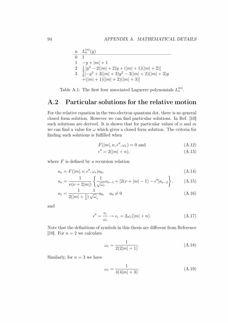
94 APPENDIX A. MATHEMATICAL DETAILS
n L|m|n (y)
0 11 −y + |m|+ 12 1
2[y2 − 2(|m|+ 2)y + (|m|+ 1)(|m|+ 2)]
3 16[−y3 + 3(|m|+ 3)y2 − 3(|m|+ 2)(|m|+ 3)y
+(|m|+ 1)(|m|+ 2)(|m|+ 3)]
Table A.1: The first four associated Laguerre polynomials L|m|n .
A.2 Particular solutions for the relative motionFor the relative equation in the two-electron quantum dot, there is no generalclosed form solution. However we can find particular solutions. In Ref. [10]such solutions are derived. It is shown that for particular values of n and mwe can find a value for ω which gives a closed form solution. The criteria forfinding such solutions is fulfilled when
F (|m|, n, ε′′, ωr) = 0 and (A.12)ε′′ = 2(|m|+ n), (A.13)
where F is defined by a recursion relation
aν = F (|m|, ν, ε′′, ωr)a0, (A.14)
aν =1
ν(ν + 2|m|)
1√ωr
aν−1 + [2(ν + |m| − 1)− ε′′]aν−2
, (A.15)
a1 =1
2(|m|+ 12)
1√ωr
a0, a0 6= 0 (A.16)
and
ε′′ =εrωr
→ εr = 2ωr(|m|+ n). (A.17)
Note that the definitions of symbols in this thesis are different from Reference[10]. For n = 2 we calculate
ωr =1
2(2|m|+ 1). (A.18)
Similarly, for n = 3 we have
ωr =1
4(4|m|+ 3). (A.19)
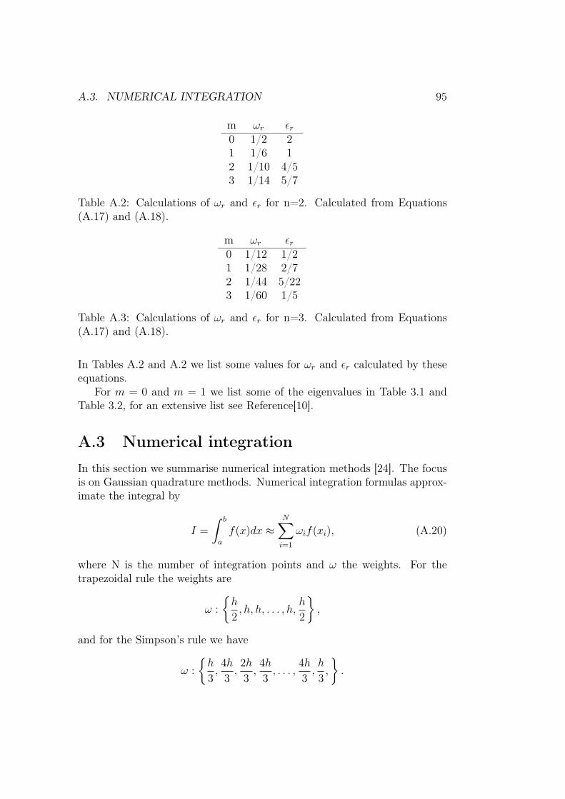
A.3. NUMERICAL INTEGRATION 95
m ωr εr0 1/2 21 1/6 12 1/10 4/53 1/14 5/7
Table A.2: Calculations of ωr and εr for n=2. Calculated from Equations(A.17) and (A.18).
m ωr εr0 1/12 1/21 1/28 2/72 1/44 5/223 1/60 1/5
Table A.3: Calculations of ωr and εr for n=3. Calculated from Equations(A.17) and (A.18).
In Tables A.2 and A.2 we list some values for ωr and εr calculated by theseequations.
For m = 0 and m = 1 we list some of the eigenvalues in Table 3.1 andTable 3.2, for an extensive list see Reference[10].
A.3 Numerical integrationIn this section we summarise numerical integration methods [24]. The focusis on Gaussian quadrature methods. Numerical integration formulas approx-imate the integral by
I =
∫ b
a
f(x)dx ≈N∑
i=1
ωif(xi), (A.20)
where N is the number of integration points and ω the weights. For thetrapezoidal rule the weights are
ω :
h
2, h, h, . . . , h,
h
2
,
and for the Simpson’s rule we have
ω :
h
3,4h
3,2h
3,4h
3, . . . ,
4h
3,h
3,
.
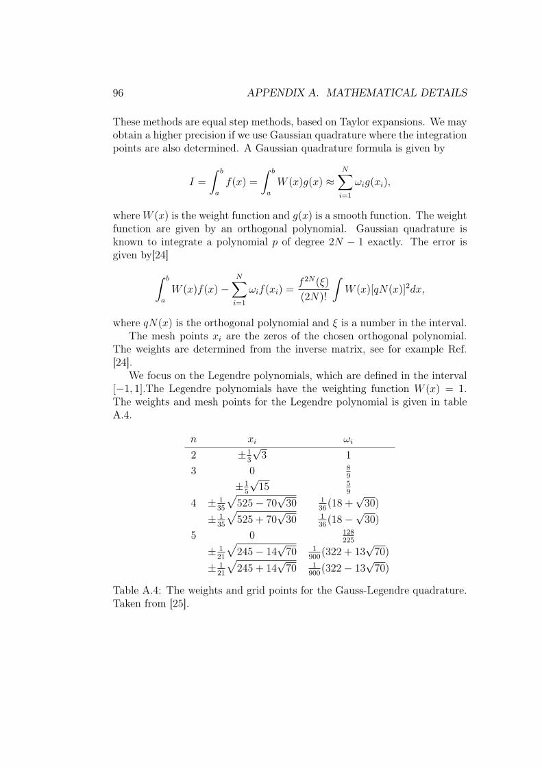
96 APPENDIX A. MATHEMATICAL DETAILS
These methods are equal step methods, based on Taylor expansions. We mayobtain a higher precision if we use Gaussian quadrature where the integrationpoints are also determined. A Gaussian quadrature formula is given by
I =
∫ b
a
f(x) =
∫ b
a
W (x)g(x) ≈N∑
i=1
ωig(xi),
where W (x) is the weight function and g(x) is a smooth function. The weightfunction are given by an orthogonal polynomial. Gaussian quadrature isknown to integrate a polynomial p of degree 2N − 1 exactly. The error isgiven by[24]∫ b
a
W (x)f(x)−N∑
i=1
ωif(xi) =f 2N(ξ)
(2N)!
∫W (x)[qN(x)]2dx,
where qN(x) is the orthogonal polynomial and ξ is a number in the interval.The mesh points xi are the zeros of the chosen orthogonal polynomial.
The weights are determined from the inverse matrix, see for example Ref.[24].
We focus on the Legendre polynomials, which are defined in the interval[−1, 1].The Legendre polynomials have the weighting function W (x) = 1.The weights and mesh points for the Legendre polynomial is given in tableA.4.
n xi ωi
2 ±13
√3 1
3 0 89
±15
√15 5
9
4 ± 135
√525− 70
√30 1
36(18 +
√30)
± 135
√525 + 70
√30 1
36(18−
√30)
5 0 128225
± 121
√245− 14
√70 1
900(322 + 13
√70)
± 121
√245 + 14
√70 1
900(322− 13
√70)
Table A.4: The weights and grid points for the Gauss-Legendre quadrature.Taken from [25].
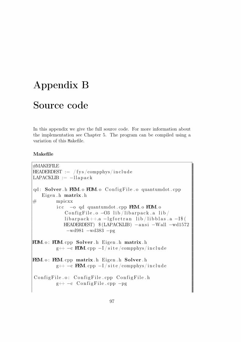
Appendix B
Source code
In this appendix we give the full source code. For more information aboutthe implementation see Chapter 5. The program can be compiled using avariation of this Makefile.
Makefile
#MAKEFILEHEADERDEST := / fy s /compphys/ inc ludeLAPACKLIB := −l l apa ck
qd : Solver . h FEM. o FDM. o Con f i gF i l e . o quantumdot . cppEigen . h matrix . h
# mpicxxi c c −o qd quantumdot . cpp FEM. o FDM. o
Con f i gF i l e . o −O3 l i b / l i ba rpack . a l i b /l i ba rpack++.a − l g f o r t r a n l i b / l i b b l a s . a −I$ (HEADERDEST) $ (LAPACKLIB) −ans i −Wall −wd1572−wd981 −wd383 −pg
FDM. o : FDM. cpp Solver . h Eigen . h matrix . hg++ −c FDM. cpp −I / s i t e /compphys/ inc lude
FEM. o : FEM. cpp matrix . h Eigen . h Solver . hg++ −c FEM. cpp −I / s i t e /compphys/ inc lude
Con f i gF i l e . o : Con f i gF i l e . cpp Con f i gF i l e . hg++ −c Con f i gF i l e . cpp −pg
97
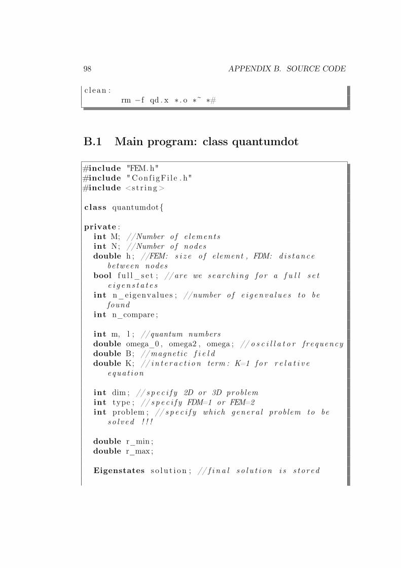
98 APPENDIX B. SOURCE CODE
c l ean :rm −f qd . x ∗ . o ∗~ ∗#
B.1 Main program: class quantumdot
#include "FEM. h"#include " Con f i gF i l e . h"#include <st r ing >
class quantumdot
private :int M; //Number o f e lementsint N; //Number o f nodesdouble h ; //FEM: s i z e o f element , FDM: d i s t ance
between nodesbool f u l l_ s e t ; // are we search ing f o r a f u l l s e t
e i g e n s t a t e sint n_eigenvalues ; //number o f e i g enva l u e s to be
foundint n_compare ;
int m, l ; //quantum numbersdouble omega_0 , omega2 , omega ; // o s c i l l a t o r f requencydouble B; //magnetic f i e l ddouble K; // i n t e r a c t i o n term : K=1 fo r r e l a t i v e
equat ion
int dim ; // s p e c i f y 2D or 3D problemint type ; // s p e c i f y FDM=1 or FEM=2int problem ; // s p e c i f y which genera l problem to be
so l v ed ! ! !
double r_min ;double r_max ;
Eigenstates s o l u t i o n ; // f i n a l s o l u t i o n i s s t o r ed
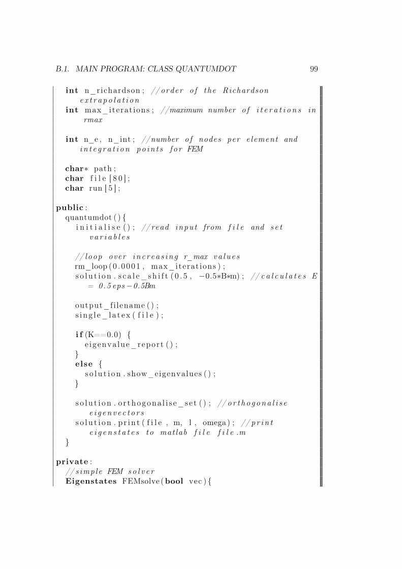
B.1. MAIN PROGRAM: CLASS QUANTUMDOT 99
int n_richardson ; // order o f the Richardsone x t r a p o l a t i o n
int max_iterat ions ; //maximum number o f i t e r a t i o n s inrmax
int n_e , n_int ; //number o f nodes per e lement andi n t e g r a t i o n po in t s f o r FEM
char∗ path ;char f i l e [ 8 0 ] ;char run [ 5 ] ;
public :quantumdot ( )
i n i t i a l i s e ( ) ; // read input from f i l e and s e tv a r i a b l e s
// loop over in c r ea s in g r_max va l u e srm_loop (0 . 0001 , max_iterat ions ) ;s o l u t i o n . s c a l e_ sh i f t ( 0 . 5 , −0.5∗B∗m) ; // c a l c u l a t e s E
= 0.5 eps−0.5Bm
output_fi lename ( ) ;s i ng l e_ l a t ex ( f i l e ) ;
i f (K==0.0) e igenva lue_report ( ) ;
else
s o l u t i o n . show_eigenvalues ( ) ;
s o l u t i o n . o r thogona l i s e_se t ( ) ; // o r t h o gona l i s ee i g en v e c t o r s
s o l u t i o n . p r i n t ( f i l e , m, l , omega ) ; // p r i n te i g e n s t a t e s to matlab f i l e f i l e .m
private :// s imple FEM so l v e rEigenstates FEMsolve (bool vec )
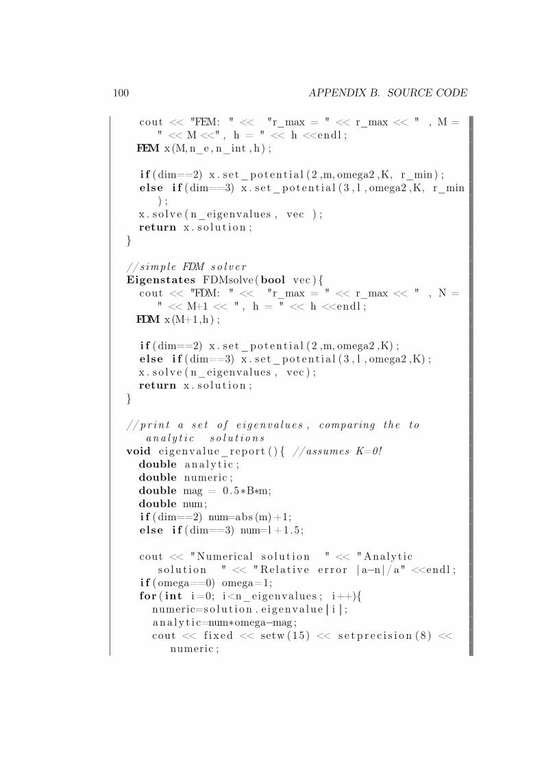
100 APPENDIX B. SOURCE CODE
cout << "FEM: " << "r_max = " << r_max << " , M =" << M <<" , h = " << h <<endl ;
FEM x (M, n_e , n_int , h ) ;
i f (dim==2) x . s e t_poten t i a l (2 ,m, omega2 ,K, r_min) ;else i f (dim==3) x . s e t_poten t i a l (3 , l , omega2 ,K, r_min
) ;x . s o l v e ( n_eigenvalues , vec ) ;return x . s o l u t i o n ;
// s imple FDM so l v e rEigenstates FDMsolve (bool vec )
cout << "FDM: " << "r_max = " << r_max << " , N =" << M+1 << " , h = " << h <<endl ;
FDM x (M+1,h) ;
i f (dim==2) x . s e t_poten t i a l (2 ,m, omega2 ,K) ;else i f (dim==3) x . s e t_poten t i a l (3 , l , omega2 ,K) ;x . s o l v e ( n_eigenvalues , vec ) ;return x . s o l u t i o n ;
// p r i n t a s e t o f e i g enva lue s , comparing the toana l y t i c s o l u t i o n s
void e igenva lue_report ( ) //assumes K=0!double ana l y t i c ;double numeric ;double mag = 0.5∗B∗m;double num;i f (dim==2) num=abs (m)+1;else i f (dim==3) num=l +1.5 ;
cout << "Numerical s o l u t i o n " << " Analyt ics o l u t i o n " << " Re la t i v e e r r o r | a−n | / a" <<endl ;
i f ( omega==0) omega=1;for ( int i =0; i<n_eigenvalues ; i++)
numeric=s o l u t i o n . e i g enva lue [ i ] ;a n a l y t i c=num∗omega−mag ;cout << f i x ed << setw (15) << s e t p r e c i s i o n (8 ) <<
numeric ;
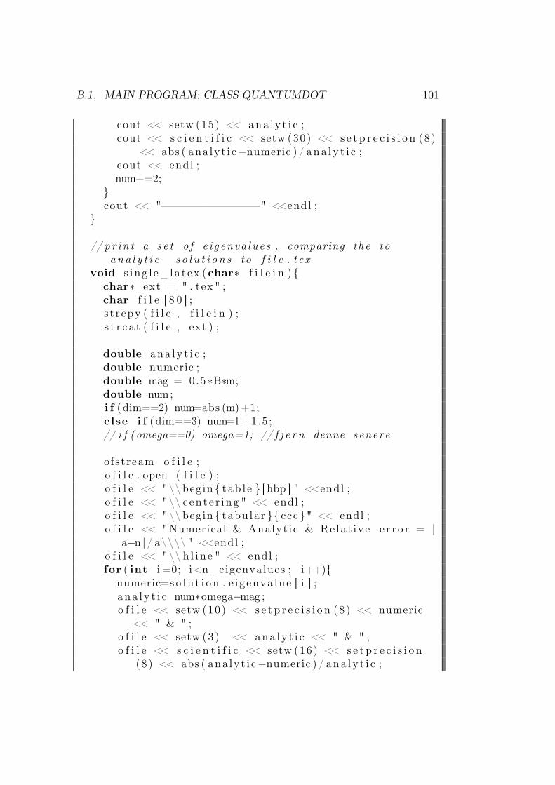
B.1. MAIN PROGRAM: CLASS QUANTUMDOT 101
cout << setw (15) << ana l y t i c ;cout << s c i e n t i f i c << setw (30) << s e t p r e c i s i o n (8 )
<< abs ( ana ly t i c−numeric ) / ana l y t i c ;cout << endl ;num+=2;
cout << "−−−−−−−−−−−−−−−" <<endl ;
// p r i n t a s e t o f e i g enva lue s , comparing the toana l y t i c s o l u t i o n s to f i l e . t e x
void s i ng l e_ l a t ex (char∗ f i l e i n ) char∗ ext = " . tex " ;char f i l e [ 8 0 ] ;s t r cpy ( f i l e , f i l e i n ) ;s t r c a t ( f i l e , ext ) ;
double ana l y t i c ;double numeric ;double mag = 0.5∗B∗m;double num;i f (dim==2) num=abs (m)+1;else i f (dim==3) num=l +1.5 ;// i f ( omega==0) omega=1; // f j e r n denne senere
ofstream o f i l e ;o f i l e . open ( f i l e ) ;o f i l e << "\\ begin tab l e [ hbp ] " <<endl ;o f i l e << "\\ c en t e r i ng " << endl ;o f i l e << "\\ begin tabu la r ccc " << endl ;o f i l e << "Numerical & Analyt ic & Re la t i v e e r r o r = |
a−n | / a\\\\" <<endl ;o f i l e << "\\ h l i n e " << endl ;for ( int i =0; i<n_eigenvalues ; i++)
numeric=s o l u t i o n . e i g enva lue [ i ] ;a n a l y t i c=num∗omega−mag ;o f i l e << setw (10) << s e t p r e c i s i o n (8 ) << numeric
<< " & " ;o f i l e << setw (3) << ana l y t i c << " & " ;o f i l e << s c i e n t i f i c << setw (16) << s e t p r e c i s i o n
(8 ) << abs ( ana ly t i c−numeric ) / ana l y t i c ;
102 APPENDIX B. SOURCE CODE
o f i l e << " \\\\ " <<endl ;o f i l e . un s e t f ( ios_base : : s c i e n t i f i c ) ;num+=2;
o f i l e << "\\end tabu la r " <<endl ;o f i l e << "\\ capt ion " << "m=" << m << " , h=" << h
<< " , $r_max$=" << r_max ;i f ( type==1) o f i l e << " ,FDM, r i c h = " <<
n_richardson ;else o f i l e <<" ,FEM, $n_e$=" << n_e << " , $n_ in t $
= " << n_int ;o f i l e <<"" <<endl ;o f i l e << "\\ l a b e l " <<endl ;o f i l e << "\\end tab l e " <<endl ;o f i l e . c l o s e ( ) ;
// read input from f i l e us ing con f i g u r a t i on manager :h t t p ://www−per sona l . umich . edu/~wagnerr/ Con f i gF i l e .html
void i n i t i a l i s e ( ) double temp ;Con f i gF i l e c on f i g ( "qd . inp " ) ;c on f i g . r eadInto ( temp , "omegainv" , 0 . 0 ) ;i f ( temp!=0) omega_0=1.0/temp ;else c on f i g . r eadInto ( omega_0 , "omega" , 1 . 0 ) ;c on f i g . r eadInto ( B, "B" , 0 . 0 ) ;c on f i g . r eadInto ( m, "m" , 1) ;c on f i g . r eadInto ( l , " l " , 1) ;c on f i g . r eadInto ( K, "K" , 0 . 0 ) ;c on f i g . r eadInto ( h , "h" , . 1 ) ;c on f i g . r eadInto ( max_iterations , "maxit" , 10) ;
// read r_max from f i l e or c a l c u l a t e , s e t Mc on f i g . r eadInto ( r_min , "r_min" , 0 . 0 ) ;c on f i g . r eadInto ( r_max , "r_max" , 0 . 0 ) ;i f (r_max==0.0) r_max=init_rmax (omega ) ;
M=( int ) c e i l (r_max/h) ;
c on f i g . r eadInto ( dim , "dim" , 2) ;i f (dim!=3) dim =2;
B.1. MAIN PROGRAM: CLASS QUANTUMDOT 103
cout << dim <<endl ;c on f i g . r eadInto ( type , " type " , 2) ;i f ( type==2)
con f i g . r eadInto ( n_e , "n_e" , 2) ;i f (n_e>3) n_e=3;c on f i g . r eadInto ( n_int , "n_int" , 5) ;N=M∗(n_e−1)+1;
else
type=1;c on f i g . r eadInto ( n_richardson , " r i c h " , 0) ;N=M+1;
// change cons tan t s f o r problem typec on f i g . r eadInto ( problem , "problem" , 0) ;i f ( problem==2) r e l a t i v e ( ) ;else i f ( problem==3) com( ) ;else i f ( problem==1) s i n g l e ( ) ;else problem=0;
// inc l ude the magnetic f i e l d in omegaomega2=omega_0∗omega_0+0.25∗B∗B;omega=sq r t ( omega2 ) ;
c on f i g . r eadInto ( fu l l_s e t , " a l l " , fa l se ) ;i f ( ! f u l l_ s e t ) c on f i g . r eadInto ( n_eigenvalues , "
num_eigenvalues" , 10) ;i f ( f u l l_ s e t ) n_eigenvalues=N−2;c on f i g . r eadInto ( n_compare , "num_eigenvalues" , 10) ;
//Output i n f o to screencout << " So lv ing : −u ’ ’ + " ;i f (dim==3) cout << " l ( l +1)" ;else cout << " (m^2−0.25)" ;cout << "u/ r^2 + w^2r^2u" ;i f (K!=0 .0) cout << "+" << K << " u/ r = eps u" ;cout << " = eps u" ;cout <<endl << "w = " << omega_0 << " , B = " << B;i f (dim==3) cout << " , l = " << l ;
104 APPENDIX B. SOURCE CODE
cout << " ,m = " << m <<endl << "Using " ;i f ( type==1) cout << "FDM, with step l ength h = " <<
h << " Richardson ex t r apo l a t i on order = " <<n_richardson <<endl ;
else cout <<"FEM, with element s i z e h = " << h << ", us ing " << n_e << " nodes per element and " <<n_int << " i n t e g r a t i o n po in t s "<<endl ;
// s e t up output f i l evoid output_fi lename ( )
path= " . . / Tekst/Double/" ; //3d /";s t r cpy ( f i l e , path ) ;
// s t r c a t ( f i l e , " r ") ;// s p r i n t f ( run , "%04.0 f " ,r_max) ;// s t r c a t ( f i l e , run ) ;// s t r c a t ( f i l e , "w") ;// s p r i n t f ( run , "%g" ,omega) ;// s t r c a t ( f i l e , run ) ;
// s t r c a t ( f i l e , "h") ;// s p r i n t f ( run , "%g" , h ) ;// s t r c a t ( f i l e , run ) ;
s t r c a t ( f i l e , "B" ) ;s p r i n t f ( run , "%g" ,B) ;s t r c a t ( f i l e , run ) ;
// s t r c a t ( f i l e , "m") ;// s p r i n t f ( run , "%i " ,m) ;// s t r c a t ( f i l e , run ) ;// s t r c a t ( f i l e , " l ") ;// s p r i n t f ( run , "%i " , l ) ;// s t r c a t ( f i l e , run ) ;
i f ( type==1) s t r c a t ( f i l e , "FDM" ) ;else
s t r c a t ( f i l e , "FEM" ) ;s p r i n t f ( run , "%i " ,n_e) ;s t r c a t ( f i l e , run ) ;
B.1. MAIN PROGRAM: CLASS QUANTUMDOT 105
cout << "Output to : " << f i l e << endl ;
// i n i t i a l i s e r_max i f not s e tint init_rmax (double omega )
double ep s i l o n =0.001;i f ( omega==0) return ( int )−l og ( e p s i l o n )+1;else return ( int ) c e i l ( s q r t (−2∗ l og ( e p s i l o n ) /omega ) )
;
// change v a r i a b l e s accord ing to problemvoid r e l a t i v e ( ) K=1; omega_0∗=0.5; void com( ) K=0; omega_0∗=2; void s i n g l e ( ) K=0;
// s o l v e f o r i n c r ea s in g r_max u n t i l the a s topp ingc r i t e r e a i s reached
// the Eigenva lues and Eigenvec tor o f the f i n a l r_maxi s s t o r ed
void rm_loop (double l im i t , int max_iterat ions )
Eigenstates temp ;int count=0;double d i f f =1;i f ( max_iterations >0)
cout <<endl<< " Sta r t i ng loop over rmax" << endl ;i f ( type==1)
i f ( n_richardson==0) s o l u t i o n=FDMsolve ( fa l se ) ;else s o l u t i o n=Richardson ( n_richardson , fa l se ) ;
i f ( type==2) s o l u t i o n=FEMsolve ( fa l se ) ;
while ( d i f f >l im i t && count<max_iterat ions )
r_max++;M=( int ) c e i l (r_max/h) ;i f ( f u l l_ s e t ) n_eigenvalues=N−2; // pass på f o r ne
! ! !
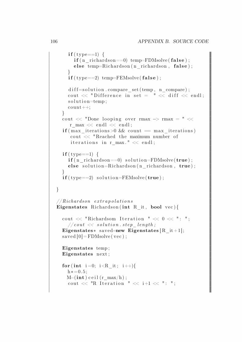
106 APPENDIX B. SOURCE CODE
i f ( type==1) i f ( n_richardson==0) temp=FDMsolve ( fa l se ) ;else temp=Richardson ( n_richardson , fa l se ) ;
i f ( type==2) temp=FEMsolve ( fa l se ) ;
d i f f=s o l u t i o n . compare_set ( temp , n_compare ) ;cout << " D i f f e r e n c e in s e t = " << d i f f << endl ;s o l u t i o n=temp ;count++;
cout << "Done loop ing over rmax −> rmax = " <<
r_max << endl << endl ;i f ( max_iterations >0 && count == max_iterat ions )
cout << "Reached the maximum number o fi t e r a t i o n s in r_max . " << endl ;
i f ( type==1) i f ( n_richardson==0) s o l u t i o n=FDMsolve ( true ) ;else s o l u t i o n=Richardson ( n_richardson , true ) ;
i f ( type==2) s o l u t i o n=FEMsolve ( true ) ;
//Richardson e x t r a p o l a t i o n sEigenstates Richardson ( int R_it , bool vec )
cout << "Richardsom I t e r a t i o n " << 0 << " : " ;// cout << so l u t i o n . s t ep_leng th ;
Eigenstates∗ saved=new Eigenstates [ R_it+1] ;saved [0 ]=FDMsolve ( vec ) ;
Eigenstates temp ;Eigenstates next ;
for ( int i =0; i<R_it ; i++)h∗=0.5;M=( int ) c e i l (r_max/h) ;cout << "R I t e r a t i o n " << i+1 << " : " ;
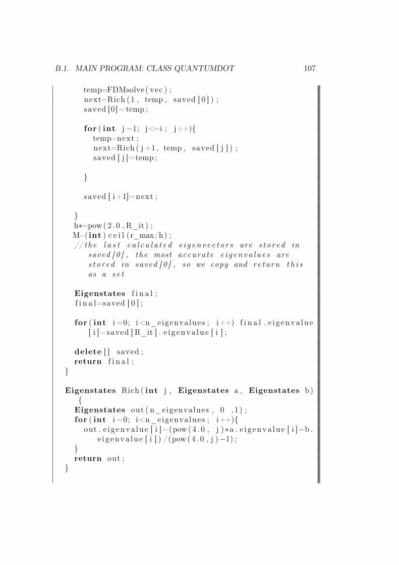
B.1. MAIN PROGRAM: CLASS QUANTUMDOT 107
temp=FDMsolve ( vec ) ;next=Rich (1 , temp , saved [ 0 ] ) ;saved [0 ]= temp ;
for ( int j =1; j<=i ; j++)temp=next ;next=Rich ( j +1, temp , saved [ j ] ) ;saved [ j ]=temp ;
saved [ i +1]=next ;
h∗=pow (2 . 0 , R_it ) ;M=( int ) c e i l (r_max/h) ;// the l a s t c a l c u l a t e d e i g en v e c t o r s are s t o r ed in
saved [ 0 ] , the most accura te e i g enva l u e s ares t o r ed in saved [ 0 ] , so we copy and re turn t h i sas a s e t
Eigenstates f i n a l ;f i n a l=saved [ 0 ] ;
for ( int i =0; i<n_eigenvalues ; i++) f i n a l . e i g enva lue[ i ]= saved [ R_it ] . e i g enva lue [ i ] ;
delete [ ] saved ;return f i n a l ;
Eigenstates Rich ( int j , Eigenstates a , Eigenstates b)
Eigenstates out ( n_eigenvalues , 0 ,1 ) ;for ( int i =0; i<n_eigenvalues ; i++)
out . e i g enva lue [ i ]=(pow ( 4 . 0 , j )∗a . e i g enva lue [ i ]−b .e i g enva lue [ i ] ) /(pow ( 4 . 0 , j )−1) ;
return out ;
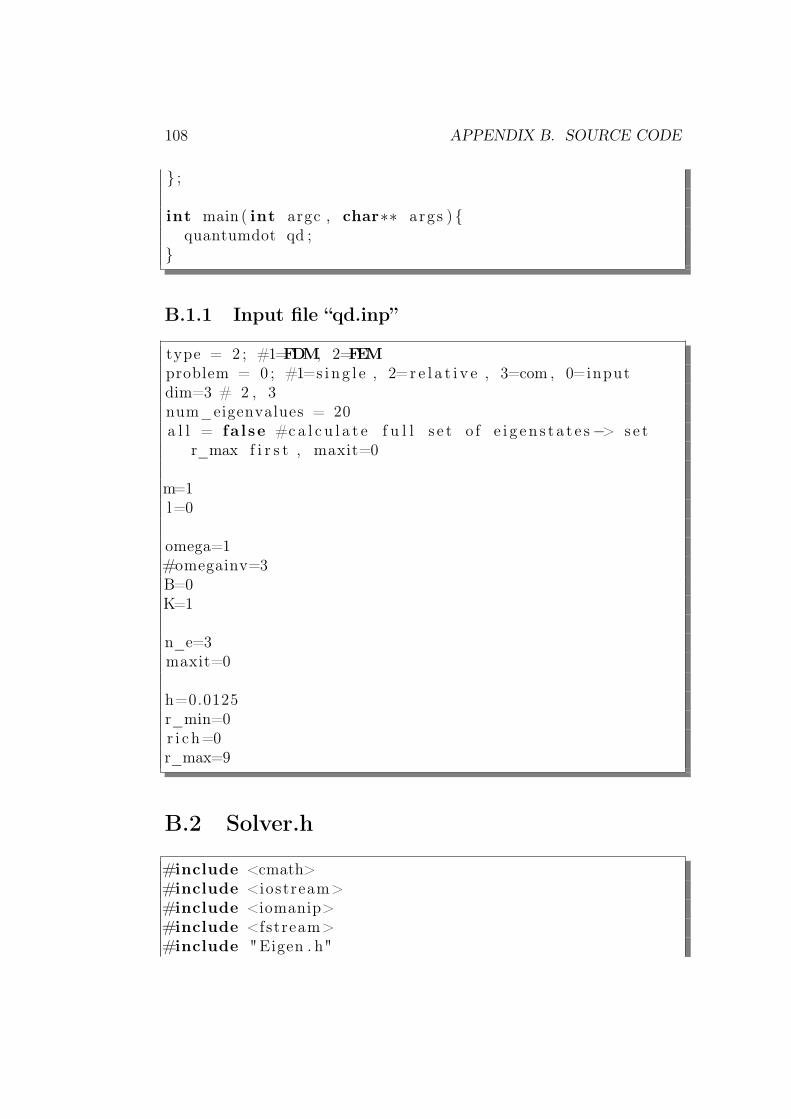
108 APPENDIX B. SOURCE CODE
;
int main ( int argc , char∗∗ args ) quantumdot qd ;
B.1.1 Input file “qd.inp”
type = 2 ; #1=FDM, 2=FEMproblem = 0 ; #1=s ing l e , 2=r e l a t i v e , 3=com , 0=inputdim=3 # 2 , 3num_eigenvalues = 20a l l = fa l se #ca l c u l a t e f u l l s e t o f e i g en s t a t e s−> se t
r_max f i r s t , maxit=0
m=1l=0
omega=1#omegainv=3B=0K=1
n_e=3maxit=0
h=0.0125r_min=0r i c h=0r_max=9
B.2 Solver.h
#include <cmath>#include <iostream>#include <iomanip>#include <fstream>#include "Eigen . h"
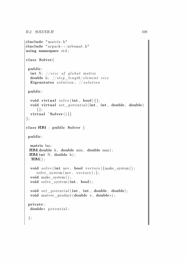
B.2. SOLVER.H 109
#include "matrix . h"#include "arpack++/arbsmat . h"using namespace std ;
class Solver
public :int N; // s i z e o f g l o b a l matrixdouble h ; // s t ep_leng th / element s i z eEigenstates s o l u t i o n ; // s o l u t i o n
public :
void virtual s o l v e ( int , bool ) ;void virtual s e t_poten t i a l ( int , int , double , double )
;virtual ~Solver ( )
;
class FDM : public Solver
public :
matrix bm;FDM(double h , double min , double max) ;FDM( int N, double h) ;~FDM( ) ;
void s o l v e ( int nev , bool vec to r s ) make_system ( ) ;solve_system ( nev , v e c t o r s ) ; ;
void make_system ( ) ;void solve_system ( int , bool ) ;
void s e t_poten t i a l ( int , int , double , double ) ;void matvec_product (double ∗ , double∗) ;
private :double∗ po t e n t i a l ;
;
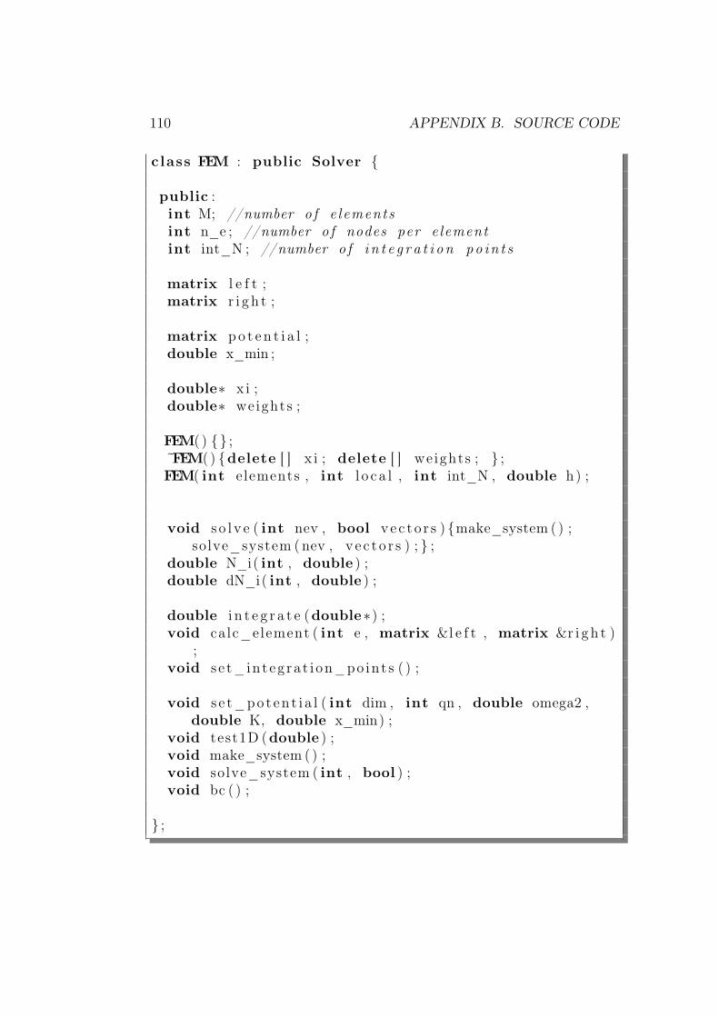
110 APPENDIX B. SOURCE CODE
class FEM : public Solver
public :int M; //number o f e lementsint n_e ; //number o f nodes per e lementint int_N ; //number o f i n t e g r a t i o n po in t s
matrix l e f t ;matrix r i g h t ;
matrix po t e n t i a l ;double x_min ;
double∗ x i ;double∗ weights ;
FEM( ) ;~FEM( ) delete [ ] x i ; delete [ ] we ights ; ;FEM( int elements , int l o c a l , int int_N , double h) ;
void s o l v e ( int nev , bool vec to r s ) make_system ( ) ;solve_system ( nev , v e c t o r s ) ; ;
double N_i( int , double ) ;double dN_i( int , double ) ;
double i n t e g r a t e (double∗) ;void calc_element ( int e , matrix &l e f t , matrix &r i gh t )
;void s e t_integ ra t i on_po int s ( ) ;
void s e t_poten t i a l ( int dim , int qn , double omega2 ,double K, double x_min) ;
void test1D (double ) ;void make_system ( ) ;void solve_system ( int , bool ) ;void bc ( ) ;
;
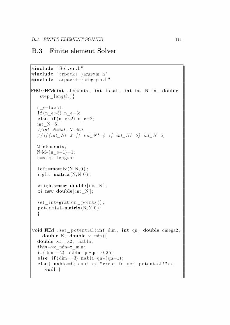
B.3. FINITE ELEMENT SOLVER 111
B.3 Finite element Solver
#include " So lve r . h"#include "arpack++/argsym . h"#include "arpack++/arbgsym . h"
FEM: :FEM( int elements , int l o c a l , int int_N_in , doublestep_length )
n_e=l o c a l ;i f (n_e>3) n_e=3;else i f (n_e<2) n_e=2;int_N=5;//int_N=int_N_in ;// i f ( int_N!=2 | | int_N!=4 | | int_N!=5) int_N=5;
M=elements ;N=M∗(n_e−1)+1;h=step_length ;
l e f t=matrix (N,N, 0 ) ;r i g h t=matrix (N,N, 0 ) ;
weights=new double [ int_N ] ;x i=new double [ int_N ] ;
s e t_integ ra t i on_po int s ( ) ;p o t e n t i a l=matrix (N,N, 0 ) ;
void FEM: : s e t_poten t i a l ( int dim , int qn , double omega2 ,double K, double x_min)
double x1 , x2 , nabla ;this−>x_min=x_min ;i f (dim==2) nabla=qn∗qn−0.25;else i f (dim==3) nabla=qn∗( qn+1) ;else nabla=0; cout << " e r r o r in s e t_poten t i a l ! "<<
endl ;
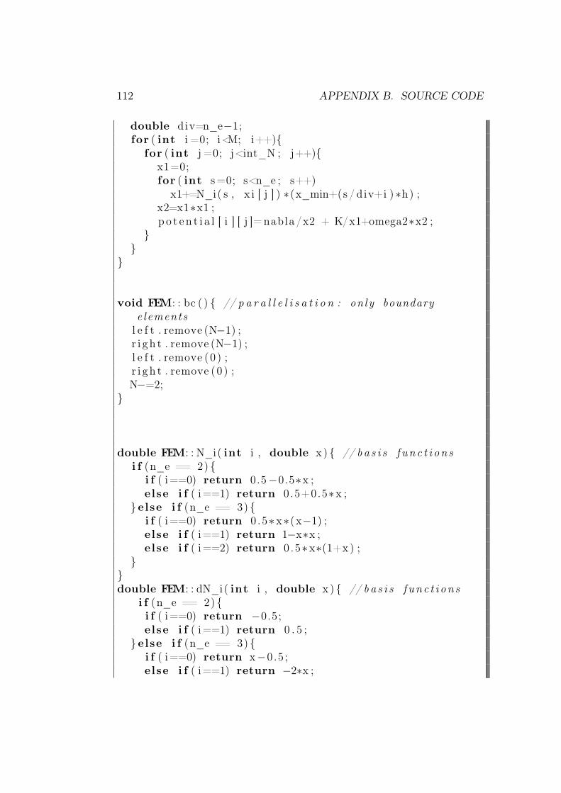
112 APPENDIX B. SOURCE CODE
double div=n_e−1;for ( int i =0; i<M; i++)
for ( int j =0; j<int_N ; j++)x1=0;for ( int s=0; s<n_e ; s++)
x1+=N_i( s , x i [ j ] ) ∗(x_min+(s / div+i )∗h) ;x2=x1∗x1 ;p o t e n t i a l [ i ] [ j ]=nabla /x2 + K/x1+omega2∗x2 ;
void FEM: : bc ( ) // p a r a l l e l i s a t i o n : on ly boundarye lements
l e f t . remove (N−1) ;r i g h t . remove (N−1) ;l e f t . remove (0 ) ;r i g h t . remove (0 ) ;N−=2;
double FEM: : N_i( int i , double x ) // b a s i s f unc t i on si f (n_e == 2)
i f ( i==0) return 0.5−0.5∗x ;else i f ( i==1) return 0.5+0.5∗x ;
else i f (n_e == 3) i f ( i==0) return 0 .5∗x∗(x−1) ;else i f ( i==1) return 1−x∗x ;else i f ( i==2) return 0 .5∗x∗(1+x) ;
double FEM: : dN_i( int i , double x ) // b a s i s f unc t i on s
i f (n_e == 2) i f ( i==0) return −0.5;else i f ( i==1) return 0 . 5 ;
else i f (n_e == 3) i f ( i==0) return x−0.5 ;else i f ( i==1) return −2∗x ;
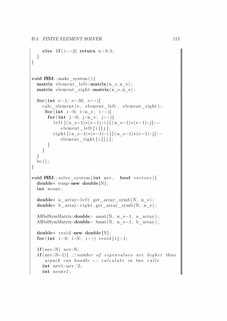
B.3. FINITE ELEMENT SOLVER 113
else i f ( i==2) return x+0.5 ;
void FEM: : make_system ( ) matrix e l ement_le f t=matrix (n_e , n_e) ;matrix e lement_right=matrix (n_e , n_e) ;
for ( int e=1; e<=M; e++)calc_element ( e , e lement_le f t , e lement_right ) ;for ( int i =0; i<n_e ; i++)for ( int j =0; j<n_e ; j++)
l e f t [ ( n_e−1)∗( e−1)+i ] [ ( n_e−1)∗( e−1)+j ]+=element_le f t [ i ] [ j ] ;
r i g h t [ ( n_e−1)∗( e−1)+i ] [ ( n_e−1)∗( e−1)+j ]+=element_right [ i ] [ j ] ;
bc ( ) ;
void FEM: : solve_system ( int nev , bool vec to r s ) double∗ temp=new double [N ] ;int nconv ;
double∗ a_array=l e f t . get_array_symb (N, n_e) ;double∗ b_array=r i gh t . get_array_symb (N, n_e) ;
ARbdSymMatrix<double> amat (N, n_e−1, a_array ) ;ARbdSymMatrix<double> bmat(N, n_e−1, b_array ) ;
double∗ r e s i d=new double [N ] ;for ( int i =0; i<N; i++) r e s i d [ i ]=1;
i f ( nev>N) nev=N;i f ( nev>N−1) //number o f e i g enva l u e s are h i ghe r than
arpack can handle −> ca l c u l a t e in two c a l l sint nev1=nev /2 ;int nconv1 ;
114 APPENDIX B. SOURCE CODE
ARluSymGenEig<double > e i g en s o l v e r 1 ( nev1 , amat ,bmat , "SM" , 0 , 0 . 0 , 0 , r e s i d , true ) ;
ARluSymGenEig<double > e i g en s o l v e r 2 ( nev−nev1 , amat ,bmat , "LM" , 0 , 0 . 0 , 0 , r e s i d , true ) ;
i f ( v e c t o r s ) nconv1 = e i g en s o l v e r 1 . FindEigenvectors ( ) ;for ( int i =0; i<N; i++) r e s i d [ i ]=1;nconv = e i g en s o l v e r 2 . FindEigenvectors ( ) ;s o l u t i o n=Eigenstates ( nev ,N, h/(n_e−1) ) ;
for ( int i =0; i<nconv1 ; i++)for ( int j =0; j<N; j++)
temp [ j ]= e i g e n s o l v e r 1 . E igenvector ( i , j ) ;s o l u t i o n . add_pair ( i , e i g e n s o l v e r 1 . Eigenvalue ( i )
, temp) ;for ( int i =0; i<nconv ; i++)
for ( int j =0; j<N; j++)
temp [ j ]= e i g e n s o l v e r 2 . E igenvector ( i , j ) ;s o l u t i o n . add_pair ( i+nconv1 , e i g e n s o l v e r 2 .
Eigenvalue ( i ) , temp) ;
else nconv1 = e i g en s o l v e r 1 . FindEigenvalues ( ) ;for ( int i =0; i<N; i++) r e s i d [ i ]=1;nconv = e i g en s o l v e r 2 . FindEigenvalues ( ) ;s o l u t i o n=Eigenstates ( nev , 0 , h/(n_e−1) ) ;for ( int i =0; i<nconv1 ; i++) s o l u t i o n . e i g enva lue [ i
]= e i g en s o l v e r 1 . Eigenvalue ( nconv1−1− i ) ;for ( int i =0; i<nconv ; i++) s o l u t i o n . e i g enva lue [ i+
nconv1 ]= e i g en s o l v e r 2 . Eigenvalue ( i ) ;
else ARluSymGenEig<double > e i g e n s o l v e r ( nev , amat , bmat ,
"SM" , 0 , 0 . 0 , 0 , r e s i d , true ) ;
i f ( v e c t o r s )
B.3. FINITE ELEMENT SOLVER 115
nconv = e i g e n s o l v e r . F indEigenvectors ( ) ;s o l u t i o n=Eigenstates ( nconv ,N, h/(n_e−1) ) ;for ( int i =0; i<nconv ; i++)
for ( int j =0; j<N; j++) temp [ j ]= e i g e n s o l v e r .E igenvector ( i , j ) ;
s o l u t i o n . add_pair ( i , e i g e n s o l v e r . Eigenvalue ( i ) ,temp) ;
else nconv = e i g e n s o l v e r . FindEigenvalues ( ) ;s o l u t i o n=Eigenstates ( nconv , 0 , h/(n_e−1) ) ;for ( int i =0; i<nconv ; i++) s o l u t i o n . e i g enva lue [ i
]= e i g e n s o l v e r . Eigenvalue ( nconv−1− i ) ;i f ( nconv<nev )
cout << "nconv<num"<<endl ;solve_system ( nev+10, v e c t o r s ) ;
delete [ ] r e s i d ;delete [ ] temp ;delete [ ] a_array ;delete [ ] b_array ;
double FEM: : i n t e g r a t e (double∗ func ) double sum=0;for ( int i =0; i<int_N ; i++)
sum+=weights [ i ]∗ func [ i ] ;return sum ;
void FEM: : ca lc_element ( int e , matrix &e l e f t , matrix &er i gh t )
double∗ i n t 1=new double [ int_N ] ;double∗ i n t 2=new double [ int_N ] ;double M_ij ;double xp ;
116 APPENDIX B. SOURCE CODE
for ( int i =0; i<n_e ; i++)for ( int j =0; j<n_e ; j++)
for ( int k=0; k<int_N ; k++)M_ij=h/2.0∗N_i( i , x i [ k ] ) ∗N_i( j , x i [ k ] ) ;i n t1 [ k]=M_ij∗ po t e n t i a l [ e−1] [ k]+ 2 .0/h∗dN_i( i , x i
[ k ] ) ∗dN_i( j , x i [ k ] ) ; ;i n t 2 [ k]=M_ij ;
e l e f t [ i ] [ j ]= i n t e g r a t e ( i n t1 ) ;e r i g h t [ i ] [ j ]= i n t e g r a t e ( i n t2 ) ;
delete [ ] i n t1 ;delete [ ] i n t2 ;
void FEM: : s e t_ integ ra t i on_po int s ( ) // h t t p :// mathworld . wolfram . com/Legendre−
GaussQuadrature . htmli f ( int_N==2)
x i [ 0 ] = −s q r t ( 1 . 0 / 3 . 0 ) ;weights [0 ]= 1 ;x i [1]=− x i [ 0 ] ;we ights [ 1 ]=1 ;
else i f ( int_N==4)
// gauss−l e g endre f o r po lynomia l o f 4 th orderx i [0 ]= −s q r t (525+70∗ s q r t (30) ) / 3 5 . 0 ;weights [0 ]= (18− s q r t (30) ) / 3 6 . 0 ;x i [1]=− s q r t (525−70∗ s q r t (30) ) / 3 5 . 0 ;weights [1]=(18+ sq r t (30) ) / 3 6 . 0 ;x i [2]=− x i [ 1 ] ;we ights [2 ]= weights [ 1 ] ;x i [3]=− x i [ 0 ] ;we ights [3 ]= weights [ 0 ] ;
else // i f ( int_N==5)// gauss−l e g endre f o r po lynomia l o f 5 th orderx i [0]=− s q r t (245+14∗ s q r t (70) ) / 2 1 . 0 ;
B.4. FINITE DIFFERENCE SOLVER 117
weights [0]=(322.0−13∗ s q r t (70) ) / 900 . 0 ;x i [1]=− s q r t (245−14∗ s q r t (70) ) / 2 1 . 0 ;weights [1 ]=(322.0+13∗ s q r t (70) ) / 900 . 0 ;x i [ 2 ]=0 ;weights [ 2 ]=128 . 0 /225 . 0 ;x i [3]=− x i [ 1 ] ;we ights [3 ]= weights [ 1 ] ;x i [4]=− x i [ 0 ] ;we ights [4 ]= weights [ 0 ] ;
B.4 Finite difference Solver
#include " So lve r . h"#include "arpack++/arssym . h"#include "arpack++/arbssym . h"
FDM: :FDM( int num_points , double s tep ) h=step ;N=num_points−2;p o t e n t i a l=new double [N ] ;bm = matrix (N,N, 0 ) ;
FDM: : ~FDM( ) delete [ ] p o t e n t i a l ;
void FDM: : s e t_poten t i a l ( int dim , int qn , double omega2 ,double K)
double h4=h∗h∗h∗h ;double nabla ;double h2=h∗h ;
i f (dim==2) nabla=qn∗qn−0.25;else i f (dim==3) nabla=qn∗( qn+1) ;else nabla=0; cout << " e r r o r in s e t_poten t i a l ! "<<
endl ;
for ( int i =1; i<=N; i++)
118 APPENDIX B. SOURCE CODE
po t e n t i a l [ i−1]=nabla /( i ∗ i )+omega2∗ i ∗ i ∗h4+ K∗h/ i ;
void FDM: : make_system ( ) for ( int i =2; i<N; i++)
bm[ i −1] [ i −1]=2 +po t en t i a l [ i −1] ;bm[ i −1] [ i ]=bm[ i −1] [ i −2]=−1;
bm[ 0 ] [ 0 ]=2 +po t en t i a l [ 0 ] ;bm[N−1] [N−1]=2 +po t en t i a l [N−1] ;bm[ 0 ] [ 1 ]= bm[N−1] [N−2]=−1;
void FDM: : solve_system ( int nev , bool vec to r s )
double h2=h∗h ;double∗ temp=new double [N ] ;int nconv ;
double∗ a_array=bm. get_array_symb (N, 2) ;ARbdSymMatrix<double> amat (N, 1 , a_array ) ;
double∗ r e s i d=new double [N ] ;for ( int i =0; i<N; i++) r e s i d [ i ]=1;
i f ( nev>N) nev=N;i f ( nev>N−1)
int nev1=nev /2 ;int nconv1 ;ARluSymStdEig<double > e i g en s o l v e r 1 ( nev1 , amat , "
SM" , 0 , 0 . 0 , 0 , r e s i d , true ) ;ARluSymStdEig<double > e i g en s o l v e r 2 ( nev−nev1 , amat ,
"LM" , 0 , 0 . 0 , 0 , r e s i d , true ) ;
i f ( v e c t o r s ) nconv1 = e i g en s o l v e r 1 . FindEigenvectors ( ) ;for ( int i =0; i<N; i++) r e s i d [ i ]=1;nconv = e i g en s o l v e r 2 . FindEigenvectors ( ) ;s o l u t i o n=Eigenstates ( nev ,N, h) ;
for ( int i =0; i<nconv1 ; i++)for ( int j =0; j<N; j++)
B.4. FINITE DIFFERENCE SOLVER 119
temp [ j ]= e i g e n s o l v e r 1 . E igenvector ( i , j ) ;s o l u t i o n . add_pair ( i , e i g e n s o l v e r 1 . Eigenvalue ( i )
/h2 , temp) ;for ( int i =0; i<nconv ; i++)
for ( int j =0; j<N; j++)
temp [ j ]= e i g e n s o l v e r 2 . E igenvector ( i , j ) ;s o l u t i o n . add_pair ( i+nconv1 , e i g e n s o l v e r 2 .
Eigenvalue ( i ) /h2 , temp) ;
else nconv1 = e i g en s o l v e r 1 . FindEigenvalues ( ) ;for ( int i =0; i<N; i++) r e s i d [ i ]=1;nconv = e i g en s o l v e r 2 . FindEigenvalues ( ) ;s o l u t i o n=Eigenstates ( nev , 0 , h ) ;for ( int i =0; i<nconv1 ; i++) s o l u t i o n . e i g enva lue [ i
]= e i g en s o l v e r 1 . Eigenvalue ( nconv1−1− i ) /h2 ;for ( int i =0; i<nconv ; i++) s o l u t i o n . e i g enva lue [ i+
nconv1 ]= e i g en s o l v e r 2 . Eigenvalue ( i ) /h2 ;
else ARluSymStdEig<double> e i g e n s o l v e r ( nev , amat , "SM" ,
0 , 0 . 0 , 0 , r e s i d , true ) ;i f ( v e c t o r s )
nconv = e i g e n s o l v e r . F indEigenvectors ( ) ;s o l u t i o n=Eigenstates ( nconv ,N, h) ;for ( int i =0; i<nconv ; i++)
for ( int j =0; j<N; j++) temp [ j ]= e i g e n s o l v e r .E igenvector ( i , j ) ;
s o l u t i o n . add_pair ( i , e i g e n s o l v e r . Eigenvalue ( i ) /h2 , temp) ;
else nconv = e i g e n s o l v e r . FindEigenvalues ( ) ;s o l u t i o n=Eigenstates ( nconv , 0 , h ) ;
120 APPENDIX B. SOURCE CODE
for ( int i =0; i<nconv ; i++) s o l u t i o n . e i g enva lue [ i]= e i g e n s o l v e r . Eigenvalue ( nconv−1− i ) /h2 ;
i f ( nconv<nev )
cout << " Inc r e a s e number o f e i g enva lu e s in searchf o r arpack . . . "<<endl ;
solve_system ( nev+10, v e c t o r s ) ;
delete [ ] r e s i d ;delete [ ] temp ;delete [ ] a_array ;
B.5 Eigenstates class
#include <iostream>#include <cmath>#include <fstream>#include <st r ing >using namespace std ;
class Eigenstates
public :int number ; //number o f e i g e n s t a t e sint l ength ; // l en g t h o f e i g en v e c t o r sdouble step_length ; // even s t ep_leng th
//quantum numbers?int∗ n ;
double∗ e i g enva lue ;double∗∗ e i g enve c t o r ;
void a l l o c a t e ( int N, int l , double h) number=N;l ength=l ;
B.5. EIGENSTATES CLASS 121
step_length=h ;
n=new int [ number ] ;e i g enva lue=new double [ number ] ;e i g enve c t o r=new double ∗ [ number ] ;for ( int i =0; i<number ; i++)
e i g enve c t o r [ i ]=new double [ l ength ] ;
void d e a l l o c a t e ( ) for ( int i =0; i<number ; i++)
delete [ ] e i g enve c t o r [ i ] ;delete [ ] e i g enva lue ;delete [ ] e i g enve c t o r ;delete [ ] n ;
Eigenstates ( ) a l l o c a t e ( 1 , 1 , 1 . 0 ) ; Eigenstates ( int N, int l , double h) a l l o c a t e (N, l , h ) ;
Eigenstates ( const Eigenstates &in )
a l l o c a t e ( in . number , in . length , in . step_length ) ;for ( int i =0; i<number ; i++)
e i g enva lue [ i ]= in . e i g enva lue [ i ] ;for ( int j =0; j<length ; j++) e i g enve c t o r [ i ] [ j ]= in .
e i g enve c t o r [ i ] [ j ] ;
~Eigenstates ( ) d e a l l o c a t e ( ) ;
Eigenstates& operator=(const Eigenstates& in ) i f ( this != &in )
i f ( number!= in . number | | l ength != in . l ength ) d e a l l o c a t e ( ) ;a l l o c a t e ( in . number , in . length , in . step_length ) ;
for ( int i =0; i<number ; i++)
e i g enva lue [ i ]= in . e i g enva lue [ i ] ;
122 APPENDIX B. SOURCE CODE
for ( int j =0; j<length ; j++) e i g enve c t o r [ i ] [ j ]=in . e i g enve c t o r [ i ] [ j ] ;
return ∗ this ;
void f ind_zeros ( ) int z e r o s ;for ( int i =0; i<number ; i++)
ze ro s =0;for ( int j =1; j<length ; j++)
i f ( ( abs ( e i g enve c t o r [ i ] [ j ]− e i g enve c t o r [ i ] [ j −1])>10e−8) && ( ( e i g enve c t o r [ i ] [ j −1] >0 &&e i g enve c t o r [ i ] [ j ]<0) | | ( e i g enve c t o r [ i ] [ j −1]<0 && e i g enve c t o r [ i ] [ j ]>0) ) )
z e r o s++;
n [ i ]= ze ro s ;
//add an e i g e n s t a t e to the s e tvoid add_pair ( int k , double val , double∗ vec )
//assumes k<number , vec [ l ]for ( int i =0; i<length ; i++)
e i g enve c t o r [ k ] [ i ]=vec [ i ] ;e i g enva lue [ k]= va l ;
// p r i n t e i g en va l u e s to screenvoid show_eigenvalues ( )
show_eigenvalues (1 ) ;
// p r i n t e i g en va l u e s s c a l e d by omega to screenvoid show_eigenvalues (double omega )
i f ( omega==0) omega=1;cout << " Eigenva lues : " <<endl ;
B.5. EIGENSTATES CLASS 123
for ( int i =0; i<number ; i++)cout << e igenva lue [ i ] / omega << endl ;
cout << "−−−−−−−−−−−−−−−" <<endl ;
// p r i n t s e i g en v e c t o r s to screen , on ly u s e f u l f o r asma l l s e t !
void pr in t_e ig envec to r s ( ) cout << " Eigenvector s " <<endl ;for ( int i =0; i<number ; i++)
for ( int j =0; j<length ; j++)cout <<e i g enve c t o r [ i ] [ j ] << " " ;
cout << endl <<endl ;
cout << "−−−−−−−−−−−−−−−" <<endl ;
// p r i n t s the s e t to a matlab s c r i p tvoid pr in t (char ∗ f i l e i n , int m, int l , double omega )
char∗ ext = " .m" ;char f i l e [ 8 0 ] ;s t r cpy ( f i l e , f i l e i n ) ;s t r c a t ( f i l e , ext ) ;
o f s tream o f i l e ;o f i l e . open ( f i l e ) ;o f i l e << "m = " << m << " ; " << endl ;o f i l e << " l = " << l << " ; " << endl ;o f i l e << "omega = " << omega << " ; " << endl ;o f i l e << "h = " << step_length << " ; " << endl ;o f i l e << "E = [ " ;for ( int i =0; i<number ; i++) o f i l e << s c i e n t i f i c <<
s e t p r e c i s i o n (21) << setw (28) << e igenva lue [ i ] ;o f i l e << " ] ; " << endl ;
o f i l e << "V = [ " <<endl ;for ( int j =0; j<length ; j++)
124 APPENDIX B. SOURCE CODE
for ( int i =0; i<number ; i++) o f i l e << s c i e n t i f i c<<s e t p r e c i s i o n (21) << setw (30) << e i g enve c t o r[ i ] [ j ] ;
o f i l e << endl ;o f i l e << " ] ; " << endl ;o f i l e . c l o s e ( ) ;
// s h i f t a l l e i g enva l u e s : v a l=va l+s h i f tvoid s h i f t (double s h i f t )
for ( int i =0; i<number ; i++)e i g enva lue [ i ] += s h i f t ;
// s c a l e a l l e i g enva l u e s : v a l=va l ∗ s c a l evoid s c a l e (double s c a l e )
for ( int i =0; i<number ; i++)e i g enva lue [ i ] ∗= s c a l e ;
// s h i f t and s c a l e a l l e i g en va l u e s va l=va l ∗ s c a l e+s h i f tvoid s c a l e_ sh i f t (double s ca l e , double s h i f t )
for ( int i =0; i<number ; i++)e i g enva lue [ i ] = s c a l e ∗ e i g enva lue [ i ]+ s h i f t ;
// dot product e i g env e c t o r ( i )∗ e i g env e c t o r ( j )double dot ( int i , int j ) // l e g g e t i l dim + r seneredouble prod=0;
for ( int k=0; k<length ; k++) //u_0 , u_N = 0prod+=e i g enve c t o r [ i ] [ k ]∗ e i g enve c t o r [ j ] [ k ] ;
prod∗=step_length ;return prod ;
B.5. EIGENSTATES CLASS 125
// normal ise e i g env e c t o r ( i )void normalise_vec ( int i ) double norm=sq r t ( dot ( i , i ) ) ;for ( int j =0; j<length ; j++)
e i g enve c t o r [ i ] [ j ]= e i g enve c t o r [ i ] [ j ] / norm ;
// normal ise a l l e i g en v e c t o r svoid normal i se ( )
for ( int i =0; i<number ; i++)normalise_vec ( i ) ;
// use the b a s i s o f e i g en v e c t o r s to c r ea t e anor thogona l s e t
void o r thogona l i s e_se t ( ) double d ;normalise_vec (0 ) ;for ( int i =1; i<number ; i++)
for ( int j =0; j<i ; j++)d=dot ( i , j ) ;for ( int k=0; k<length ; k++)
e i g enve c t o r [ i ] [ k]−=d∗ e i g enve c t o r [ j ] [ k ] ;normalise_vec ( i ) ;
//compare the n_compare f i r s t e i g en va l u e s to s e t b ,r e tu rn ing sum | a_i−b_i | , used i rm_loop iquantumdot . cpp , compare a l go may be improved tocheck the convergence o f e i g enva l u e (n_compare )
double compare_set ( Eigenstates b , int n_compare ) double e r r o r =0;n_compare = min (min (n_compare , number ) , b . number ) ;for ( int i =0; i<n_compare ; i++)
e r r o r+=abs ( e i g enva lue [ i ]−b . e i g enva lue [ i ] ) ;
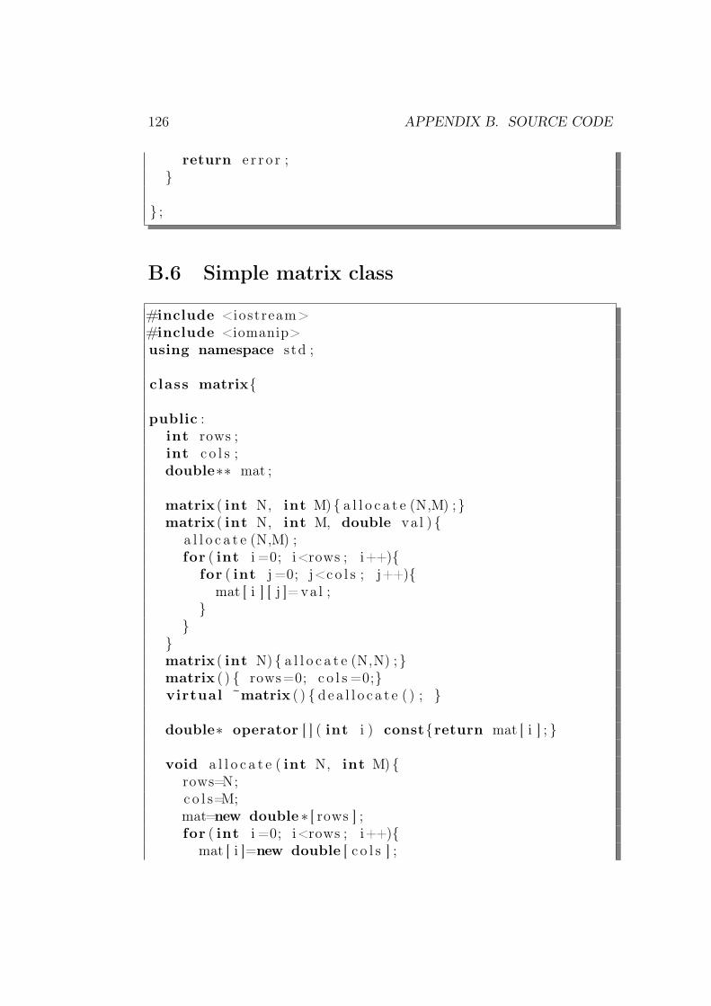
126 APPENDIX B. SOURCE CODE
return e r r o r ;
;
B.6 Simple matrix class
#include <iostream>#include <iomanip>using namespace std ;
class matrix
public :int rows ;int c o l s ;double∗∗ mat ;
matrix ( int N, int M) a l l o c a t e (N,M) ; matrix ( int N, int M, double va l )
a l l o c a t e (N,M) ;for ( int i =0; i<rows ; i++)
for ( int j =0; j<c o l s ; j++)mat [ i ] [ j ]= va l ;
matrix ( int N) a l l o c a t e (N,N) ; matrix ( ) rows=0; c o l s =0;virtual ~matrix ( ) d e a l l o c a t e ( ) ;
double∗ operator [ ] ( int i ) constreturn mat [ i ] ;
void a l l o c a t e ( int N, int M)rows=N;c o l s=M;mat=new double ∗ [ rows ] ;for ( int i =0; i<rows ; i++)
mat [ i ]=new double [ c o l s ] ;
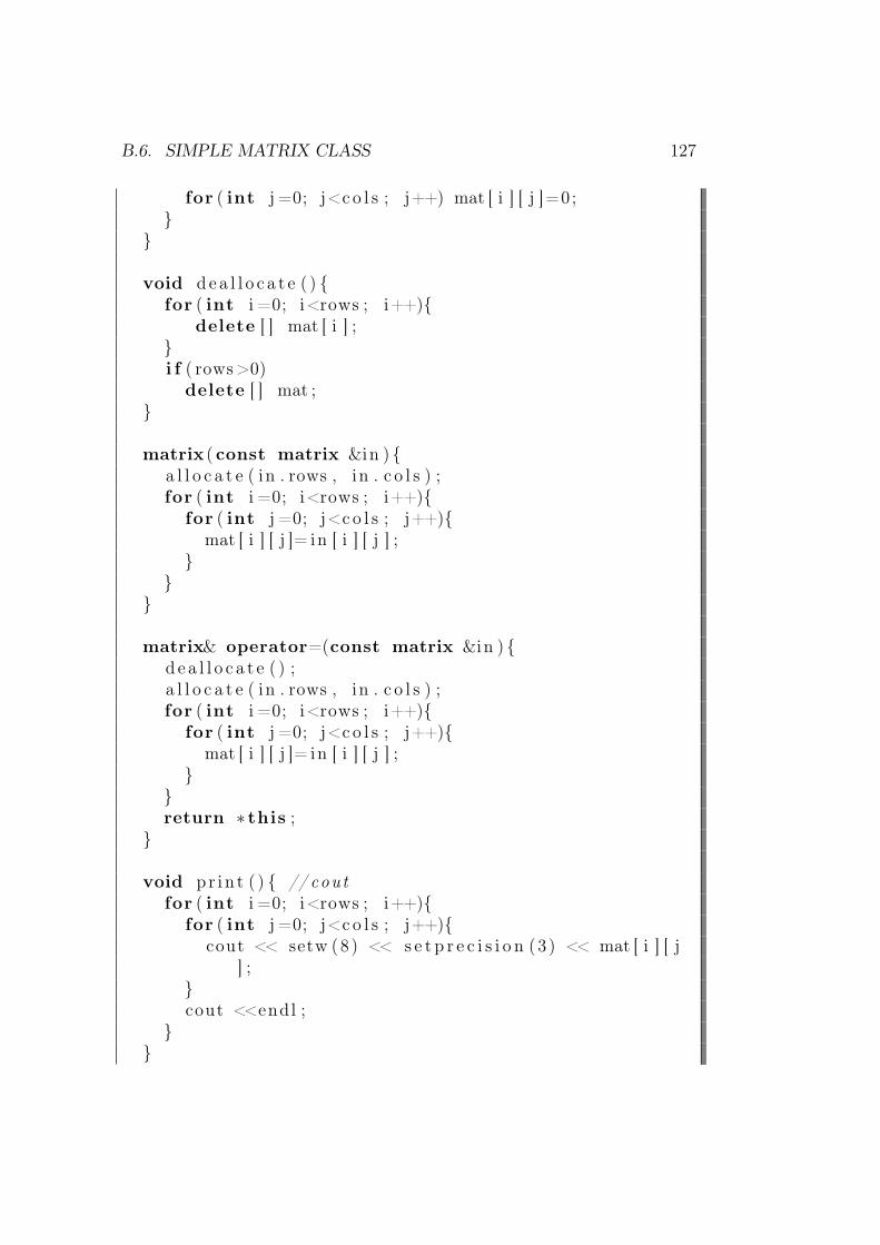
B.6. SIMPLE MATRIX CLASS 127
for ( int j =0; j<c o l s ; j++) mat [ i ] [ j ]=0;
void d e a l l o c a t e ( ) for ( int i =0; i<rows ; i++)
delete [ ] mat [ i ] ;i f ( rows>0)
delete [ ] mat ;
matrix ( const matrix &in ) a l l o c a t e ( in . rows , in . c o l s ) ;for ( int i =0; i<rows ; i++)
for ( int j =0; j<c o l s ; j++)mat [ i ] [ j ]= in [ i ] [ j ] ;
matrix& operator=(const matrix &in ) d e a l l o c a t e ( ) ;a l l o c a t e ( in . rows , in . c o l s ) ;for ( int i =0; i<rows ; i++)
for ( int j =0; j<c o l s ; j++)mat [ i ] [ j ]= in [ i ] [ j ] ;
return ∗ this ;
void pr in t ( ) // coutfor ( int i =0; i<rows ; i++)
for ( int j =0; j<c o l s ; j++)cout << setw (8) << s e t p r e c i s i o n (3 ) << mat [ i ] [ j
] ;cout <<endl ;
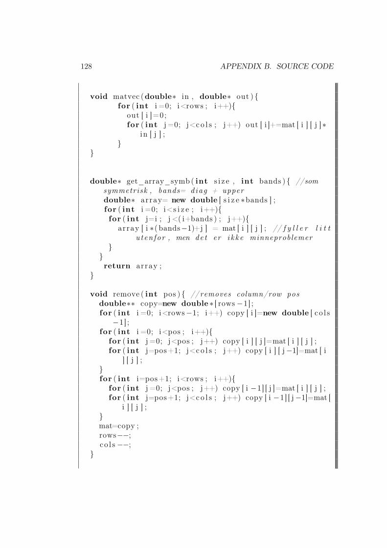
128 APPENDIX B. SOURCE CODE
void matvec (double∗ in , double∗ out ) for ( int i =0; i<rows ; i++)
out [ i ]=0;for ( int j =0; j<c o l s ; j++) out [ i ]+=mat [ i ] [ j ]∗
in [ j ] ;
double∗ get_array_symb ( int s i z e , int bands ) //somsymmetrisk , bands= diag + upperdouble∗ array= new double [ s i z e ∗bands ] ;for ( int i =0; i<s i z e ; i++)for ( int j=i ; j <( i+bands ) ; j++)
array [ i ∗( bands−1)+j ] = mat [ i ] [ j ] ; // f y l l e r l i t tu tenfor , men de t er i k k e minneproblemer
return array ;
void remove ( int pos ) // removes column/row posdouble∗∗ copy=new double ∗ [ rows −1] ;for ( int i =0; i<rows−1; i++) copy [ i ]=new double [ c o l s
−1] ;for ( int i =0; i<pos ; i++)
for ( int j =0; j<pos ; j++) copy [ i ] [ j ]=mat [ i ] [ j ] ;for ( int j=pos+1; j<c o l s ; j++) copy [ i ] [ j−1]=mat [ i
] [ j ] ;for ( int i=pos+1; i<rows ; i++)
for ( int j =0; j<pos ; j++) copy [ i −1] [ j ]=mat [ i ] [ j ] ;for ( int j=pos+1; j<c o l s ; j++) copy [ i −1] [ j−1]=mat [
i ] [ j ] ;mat=copy ;rows−−;c o l s −−;
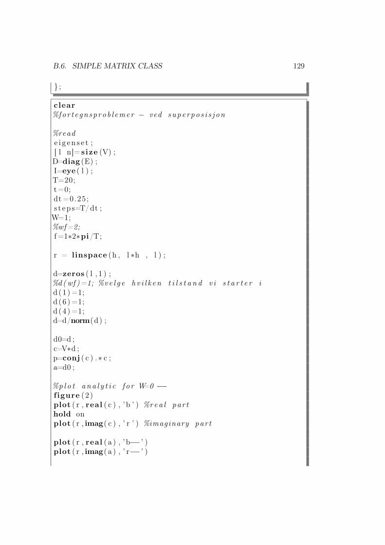
B.6. SIMPLE MATRIX CLASS 129
;
clear%for t e gnsprob l emer − ved supe rpo s i s j on
%reade i g e n s e t ;[ l n]= s ize (V) ;D=diag (E) ;I=eye ( l ) ;T=20;t=0;dt =0.25;s t ep s=T/dt ;
W=1;%wf=2;f =1∗2∗pi/T;
r = linspace (h , l ∗h , l ) ;
d=zeros ( l , 1 ) ;%d(wf )=1; %v e l g e h v i l k e n t i l s t a n d v i s t a r t e r id (1) =1;d (6 ) =1;d (4 ) =1;d=d/norm(d) ;
d0=d ;c=V∗d ;p=conj ( c ) .∗ c ;a=d0 ;
%p l o t ana l y t i c f o r W=0 −−f igure (2 )plot ( r , real ( c ) , ’ b ’ ) %rea l par thold onplot ( r , imag( c ) , ’ r ’ ) %imaginary par t
plot ( r , real ( a ) , ’b−− ’ )plot ( r , imag( a ) , ’ r−− ’ )
130 APPENDIX B. SOURCE CODE
plot ( r , p , ’ g ’ ) % c∗cylim ( [ −1 ,1 ] ) ;hold o f fMovie (1 )=getframe ;
for j =0: steps−1 %evo l v e from t j to t j+1
%H( s )i n t 1=D∗dt+I∗−W∗( cos ( f ∗( t+dt ) )−cos ( f ∗ t ) ) / f ;%sH( s )i n t 2=D∗dt ∗( t +0.5∗dt )+I ∗W∗( sin ( f ∗( t+dt ) )−t∗ f ∗cos ( f ∗( t
+dt ) )−sin ( f ∗dt )+t∗ f ∗cos ( f ∗dt ) ) / f / f ;
H0=−i ∗ i n t 1 ;H1=i /dt ∗ ( ( t +0.5∗dt )∗ int1−i n t 2 ) ;
d=expv(−1 , H1 , d) ;d=expv (1 , H0 , d) ;d=expv (1 , H1 , d) ;
t=t+dt ;c=V∗d ;p=conj ( c ) .∗ c ;
a=V∗diag (exp(− i ∗E∗ t ) )∗d0 ;d i f f=c−a ;sum( d i f f ) ; %sammenlikne med ana l y t i s k f o r W=0
plot ( r , real ( c ) , ’ b ’ )hold onplot ( r , imag( c ) , ’ r ’ )plot ( r , real ( a ) , ’b−− ’ )%hold onplot ( r , imag( a ) , ’ r−− ’ )plot ( r , p , ’ g ’ )text (10∗h , 0 . 8 , [ ’ t=’ , num2str( t ) ] )hold o f fyl im ( [ −1 ,1 ] ) ;Movie ( j +2)=getframe ;%sin ( f ∗ t )

B.6. SIMPLE MATRIX CLASS 131
end
%movie (Movie , 1 , 1 )

Bibliography
[1] David j. Griffiths. Introduction to Quantum Mechanics. Pearson, 2005.
[2] R. Shankar. Principles of Quantum Mechanics. Plenum Press, 1994.
[3] Finn Ravndal. Notes on quantum mechanics. Lecture notes - FYS 3110.
[4] NIST (National Institute og Standards and Technology). Codata inter-nationally recommended values of the fundamental physical constants.
[5] Eric W. Weisstein. Legendre polynomial. From MathWorld–A Wolframweb resource http://mathworld.wolfram.com/LegendrePolynomial.html.
[6] Stephanie M. Reimann and Matti Manninen. Electronic structure ofquantum dots. Rev. Mod. Phys, 74:1283, 2002.
[7] R. C. Ashoori. Electrons in artificial atoms. Nature, 379:413, 1996.
[8] Daniel Loss and David P. DiVincenzo. Quantum computation withquantum dots. Phys. Rev. A, 57(1):120–126, Jan 1998.
[9] Xiaohu Gao, Yuanyuan Cui, Richard M. Levenson, Leland W K . Chung,and Shuming Nie. In vivo cancer targeting and imaging with semicon-ductor quantum dots. nature biotechnology, 22(8):969, August 2004.
[10] M. Taut. Two electrons in a homogeneous magnetic field: particularanalytical solutions. J. Phys. A: Math. Gen., 27:1045, 1994.
[11] M. Taut. Two electrons in an external oscillator potential: Particu-lar analytic solutions of a coulomb correlation problem. Phys. Rev. A,48(5):3561–3566, Nov 1993.
[12] Andreassen et al. Numeriske metoder. Tapir, 1986.
[13] H.P. Langtangen. Computational Partial Differential Equations: Nu-merical Methods and Diffpack Programming. Springer, 2003.
133
134 BIBLIOGRAPHY
[14] L. Ramdas Ram-Mohan. Finite Element and Boundary Element Appli-cations in Quantm Mechanics. Oxford University Press, 2002.
[15] H.P. Langtangen and A. Tveito. Advanced topics in computational par-tial differential equations: numerical methods and diffpack programming.Springer, 2003.
[16] S Blanes and P. C. Moan. Splitting methods for the time-dependentSchrödinger equation. Physics Letters A, 265:35–42, 2000.
[17] W.H. Press, B.P. Flannery, S.A. Teukolsky, and W.T. Vetterling. Nu-merical Recipes in C++, The art of scientific Computing. CambridgeUniversity Press, 1999.
[18] Arpack software. http://www.caam.rice.edu/software/ARPACK/.
[19] G.H. Golub and C.F. Van Loan. Matrix Computations. John HopkinsUniversity Press, 1996.
[20] Simen. Kvaal. A critical study of the finite difference and finite elementmethods for the time dependent Schrödinger equation. Master’s thesis,University of Oslo, 2004.
[21] Rick Wagner. Configuration file reader for c++. http://www-personal.umich.edu/~wagnerr/ConfigFile.html.
[22] Expokit - matrix exponential software package for dense and sparse ma-trices. http://www.maths.uq.edu.au/expokit/.
[23] Eric W. Weisstein. Laguerre polynomial. From MathWorld–A Wolframweb resource http://mathworld.wolfram.com/LaguerrePolynomial.html.
[24] Morten. Hjorth-Jensen. Lecture notes on computational physics.http://www.uio.no/studier/emner/matnat/fys/FYS3150/h08/undervisningsmateriale/Lecture%20Notes/lecture2008.pdf,2006. Lecture notes in FYS-3150 and FYS 4410.
[25] Eric W. Weisstein. Legendre-gauss quadrature. From MathWorld–A Wolfram web resource http://mathworld.wolfram.com/Legendre-GaussQuadrature.html.