Finite-element modelling oftympanic-membrane vibrationsunder quasi-static pressurization

Sahar Choukir

Department of BioMedical Engineering

McGill University, Montréal

August 2017

A thesis submitted to McGill University

in partial fulfillment of the requirements of the degree of

Master of Engineering

©Sahar Choukir, 2017

Finite-element modelling oftympanic-membrane vibrationsunder quasi-static pressurization

AbstractEarly detection of hearing loss is important so it can be addressed in a timely manner. Current newborn

hearing screening methods produce high false-positive rates which are attributed to transient conditions

in the external and middle ear in the first 48 hours after birth. Tympanometry (acoustical input

admittance measurement in the presence of a range of quasi-static pressures) is a promising tool for

characterizing middle-ear status in newborns but their response to tympanometry is not well

understood. Tympanometry involves large, nonlinear deformations; viscoelastic (time-dependent)

effects; and complex dynamic responses. The goal of this study is to combine these three features in a

dynamic nonlinear viscoelastic model. The constitutive equation of this model is a convolution integral

composed of a Mooney-Rivlin hyperelastic model and an exponential time-dependent Prony series with

six time constants. Material properties are taken from previous measurements and estimates. The

tympanic membrane contributes to the overall response more than other middle-ear components do and

those other components are greatly simplified in this model. The tympanic membrane is assumed to be

homogeneous and nearly incompressible. The loading conditions included low-amplitude sound

pressures; high quasi-static pressures; and combinations of high quasi-static pressures with low-

amplitude sound pressures, corresponding to those involved in tympanometry. Simulations were

performed with two different finite-element solvers and we report simulated displacements and

vibrations in the frequency and time domains for the different loading conditions. Results from the two

finite-element solvers were compared and were similar. The simulation results were compared with

measured data from experimental animals. In response to high quasi-static pressures, the model

i

replicates the asymmetrical effects of positive and negative pressures on the displacement; the

hysteresis of the displacement; and the frequency dependence of the hysteresis. The model also

replicates the differences between the peak-admittance magnitudes and the pressures at which they

occur for low-amplitude vibrations during negative and positive sweeps of high quasi-static pressures.

Our dynamic nonlinear viscoelastic model of the middle ear permits quantitative insights into the

middle ear’s response to different loading conditions and will help to establish improved applications

of tympanometric measurements in newborns.

ii

Modélisation par éléments finis des

vibrations de la membrane tympanique

mise en pression quasi statique

RésuméLa détection précoce de la perte auditive est très importante pour une intervention précoce appropriée.

Les méthodes de dépistage de perte d’audition actuelles pour les nouveau-nés produisent des taux

élevés de faux positifs que l’on attribue au régime transitoire qui prévaut dans l'oreille externe et

l’oreille moyenne dans les premières 48 heures postnatales. La tympanométrie (la mesure de

l’admittance d'entrée acoustique en présence de pressions quasi statiques) est un outil prometteur pour

évaluer l'état de l'oreille moyenne chez les nouveau-nés, mais, leur réponse à la tympanométrie n'est

pas bien comprise. La tympanométrie comprend de grandes déformations nonlinéaires; des effets

viscoélastiques (dépendants du temps); et des réponses dynamiques complexes. L’objectif de cette

étude est de combiner ces trois caractéristiques dans un modèle dynamique viscoélastique nonlinéaire.

L’équation constitutive de ce modèle est une intégrale de convolution composée d’un modèle

hyperélastique Mooney-Rivlin et de la fonction exponentielle dépendante du temps de la série de Prony

avec six constantes temporelles. Les propriétés des matériaux sont déterminées avec des mesures et des

estimations antérieures. La membrane tympanique contribue davantage à la réponse globale que les

autres composantes de l’oreille moyenne et ces autres composantes sont simplifiés dans ce modèle. La

membrane tympanique est supposée homogène et quasi incompressible. Les conditions de chargement

comprenaient des pressions sonores à faible amplitude; pressions quasi statiques élevées; et des

combinaisons de pressions quasi statiques élevées avec des pressions sonores à faible amplitude,

correspondant à celles impliquées dans la tympanométrie. Des simulations ont été effectuées avec deux

solveurs d’éléments finis différents et nous signalons les déplacements simulés et les vibrations dans

iii

les domaines de fréquence et du temps pour les différentes conditions de chargement. Les résultats des

deux solveurs à éléments finis ont été comparés et étaient similaires. Les résultats de la simulation ont

été comparés aux données expérimentales provenant d’animaux. En réponse à des pressions quasi

statiques élevées, le modèle réplique les effets asymétriques des pressions positives et négatives sur le

déplacement; l’hystérésis du déplacement; et la dépendance en fréquence de l'hystérésis. Le modèle

réplique également les différences entre les magnitudes d'admission maximum et les pressions à

laquelle elles se produisent pour des vibrations de faible amplitude lors de balayages négatifs et positifs

de pressions quasi statiques élevées. Nos modèles numériques dynamiques viscoélastiques et

nonlinéaires de la membrane tympanique fournissent une piste pour étudier la mécanique de l’oreille

moyenne en réponse à différentes conditions de chargements et, en particulier, établissent les bases

pour améliorer l’application clinique des mesures tympanométriques chez les nouveau-nés.

iv

AcknowledgementsI would like to thank all the people who contributed in some way to the work described in this thesis.

First of all, I would like to express my deep appreciation for my supervisor Dr. W. Robert J. Funnell for

accepting me into his group, his guidance and unfailing support and contribution of ideas in preparing

this thesis, and his patience in reviewing my work.

I must also acknowledge Dr. Willem F. Decraemer of the University of Antwerp, Belgium. His smart

comments and valuable feedback on my model were of great assistance when analyzing my results.

The past and present members of the Auditory Mechanics Laboratory have contributed immensely to

my personal and professional time at McGill. I would like to acknowledge Nima and Hamid, for their

prompt help to explain their previous work in the lab, provide constructive advice and their willingness

to help. I thank Orhun for conducting measurements for validation of my simulations on very short

notice even though we didn’t end up using the data. I would also like to thank Majid for his help in

explaining some concepts to me and for other valuable input. I am also very thankful to Xuan for her

great personality, her kindness and her sense of humour.

I am deeply indebted to my parents Jamel and Najoua, and my brothers Omar, Makram and Racem for

their constant love and support. Without them, I would not have been be able to finish up my thesis.

My gratitude also goes to all those who, formally and informally, gave me the benefit of their

knowledge, views and experience. I am also indebted to all of our friends for their moral support and

encouragement during the preparation of this dissertation.

My sincere thanks also go to Pina Sorrini, Daniel Caron and Trang Q. Tran. Their guidance and support

during my studies have been very valuable.

This work was supported by the Canadian Institutes of Health Research, the Natural Sciences and

Engineering Council of Canada and the BioMedical Engineering Department.

v

Table of ContentsAcknowledgements...................................................................................................................................vChapter1: Introduction...........................................................................................................................1

1.1 Motivation..........................................................................................................................................11.2 Objectives..........................................................................................................................................21.3 Thesis outline.....................................................................................................................................3

Chapter 2: The auditory system.............................................................................................................42.1 Introduction........................................................................................................................................42.2 Anatomy of outer ear.........................................................................................................................42.3 Anatomy of middle ear......................................................................................................................5

2.3.1 Tympanic membrane....................................................................................................................52.3.2 Ossicles.........................................................................................................................................72.3.3 Ligaments and muscles................................................................................................................82.3.4 Middle-ear cavity.........................................................................................................................9

2.4 Anatomy of inner ear.......................................................................................................................102.4 Gerbil middle ear.............................................................................................................................11

Chapter 3: Literature review................................................................................................................133.1 Introduction......................................................................................................................................133.2 Tympanometry.................................................................................................................................13

3.2.1 Principles of tympanometry.......................................................................................................133.2.2 Clinical applications of tympanometry......................................................................................173.2.3 Tympanometry in newborns.......................................................................................................19

3.3 Finite-element method.....................................................................................................................223.3.1 Introduction................................................................................................................................223.3.2 Nonlinear and time-dependent material models.........................................................................25

3.3.2.1 Finite-strain theory................................................................................................................263.3.2.2 Hyperelasticity......................................................................................................................273.3.2.3 Viscoelasticity.......................................................................................................................283.3.2.4 Viscoelasticity and nonlinearity in the middle ear................................................................32

3.3.3 Finite-element models of the ear................................................................................................383.4 Experimental measurements............................................................................................................43

3.4.1 Measurements of non-gerbil tympanic-membrane vibrations....................................................433.4.2 Unpressurized vibration measurements in gerbils......................................................................463.4.3 Static pressure deformations......................................................................................................473.4.4 Pressurized TM vibrations..........................................................................................................52

3.4.4.1 Tympanometric measurements..............................................................................................523.4.4.2 Laser Doppler vibrometry measurements.............................................................................53

Chapter 4: Methods...............................................................................................................................564.1 Introduction......................................................................................................................................564.2 Geometry, model components and mesh.........................................................................................564.3 Boundary conditions........................................................................................................................614.4 Material Properties...........................................................................................................................62

4.4.1 Tympanic membrane..................................................................................................................624.4.1.1 Governing equations.............................................................................................................624.4.1.2 Viscoelastic parameters.........................................................................................................66

vi

4.4.1.3 Hyperelastic parameters........................................................................................................684.4.2 Manubrium, wedge and block....................................................................................................704.4.3 Cochlear load..............................................................................................................................71

4.5 Loading conditions and time-step analysis......................................................................................724.6 Mesh convergence...........................................................................................................................77

Chapter 5: Results..................................................................................................................................795.1 Introduction......................................................................................................................................795.2 Unpressurized vibrations.................................................................................................................79

5.2.1 Comparison of FEBio and Code_Aster......................................................................................795.2.2 Umbo and pars-flaccida responses.............................................................................................82

5.2.2.1 Low frequencies....................................................................................................................825.2.2.2 Mid and high frequencies......................................................................................................86

5.2.3 Manubrial response....................................................................................................................895.2.4 Pars-tensa response.....................................................................................................................91

5.3 Pressurized vibrations......................................................................................................................935.3.1 Triangular quasi-static pressure signals......................................................................................93

5.3.1.1 Displacement versus quasi-static pressure............................................................................935.3.1.2 Vibration amplitude versus quasi-static pressure................................................................102

5.3.2 Sinusoidal static pressure signals.............................................................................................1065.3.3 Ramp static pressure signals combined with low-amplitude sound pressures.........................1095.3.4 Discussion.................................................................................................................................112

Chapter 6: Conclusion.........................................................................................................................1176.1 Summary........................................................................................................................................1176.2 Future work....................................................................................................................................1196.3 Significance...................................................................................................................................122

References.............................................................................................................................................123

vii

Chapter1: Introduction

1.1 MotivationHearing loss is one of the most common birth defects – about 3 in 1000 babies are born with some

degree of hearing impairment. Early detection of hearing loss accompanied by appropriate early

intervention is important in order to avoid problems associated with language development that affect

daily communication, educational achievement, psychosocial development, and quality of life in

general. Currently, otoacoustic emission (OAE) and/or auditory brainstem response (ABR) tests are

employed as screening tools in newborn hearing screening programs. However, they have high

false-positive rates that are often attributed to transient conditions in the middle ear due to fluid and

other residual material in the first 48 hours after birth, which conflicts with the desire for in-hospital

screening and shorter hospital stays.

Admittance measurement is a promising tool for assessing middle-ear status in newborns. In this

method, the acoustical input admittance of the outer and middle ear is measured in response to an

acoustical excitation, which can be either single-frequency or wideband. Tympanometry provides

additional information by introducing a range of quasi-static air pressures in the ear canal along with

the acoustical excitation. Low-frequency tympanometry with a single probe-tone frequency provides

easy-to-interpret results for adult ears, but the results in newborns are very different from those in

adults. Differences in the interpretation of results in adults and newborns may be attributed to

anatomical and physiological changes during maturation. More information can be obtained quickly

over a broad frequency range by using a wideband stimulus, but the wideband admittance response of

the infant ear is even less well understood. Furthermore, many procedural variables, including the

direction and rate of the quasi-static pressurization and the frequencies of the acoustical stimulus,

influence tympanometric results. It is unclear exactly how these variables affect tympanometry and

1

what their clinical significance is.

Understanding and predicting the response of the middle ear to tympanometry can be facilitated by

developing numerical models of the middle ear. Such models allow us to study the effects of different

parameters quantitatively to get a better understanding of their roles. Different approaches to modelling

the middle ear were reviewed by Funnell et al. (2012) and are discussed briefly in section 3.3.3.

Finite-element models allow us to connect the detailed anatomical and mechanical properties of the

middle-ear structures to the physiological characteristics of the system. In recent years, the

finite-element method has been increasingly applied in modelling of the middle ear due to the

increasing accessibility of finite-element preprocessing programmes and solvers.

1.2 ObjectivesTympanometry involves both nonlinear responses and viscoelastic (time-dependent) effects. To the best

of our knowledge, no previous numerical models have addressed the dynamic response of the middle

ear in the presence of both quasi-static pressures and acoustical stimuli (comparable to those in

tympanometry) while accounting for both nonlinearity and viscoelasticty. The research conducted here

forms part of a research programme that has as its goal an improved understanding of tympanometry in

newborns. In this research, an animal model (the Mongolian gerbil ear) is used because it allows

comparison with experimental measurements that are not possible with human ears. The overall

objective of my thesis is to develop a better quantitative understanding of the mechanical behaviour of

the gerbil middle ear, particularly its response under conditions involving both nonlinear viscoelasticity

and linear dynamics as found in tympanometry. The specific objectives of my thesis are listed below:

1. Development of a dynamic, nonlinear viscoelastic model for the gerbil middle ear, with the

material properties of the different components estimated from previous work.

1. Investigation of the behaviour of the model in conditions relevant to tympanometry, involving

2

the presence of large quasi-static ear-canal pressures with and without the presence of a sound

stimulus.

2. Comparison of the model results with experimental measurements.

1.3 Thesis outlineChapter 2 of the thesis is a basic overview of the auditory system with emphasis on the anatomy of the

middle ear. Chapter 3 consists of a literature review of concepts and previous studies related to the

present work. The methods are presented in Chapter 4, followed by our results in Chapter 5. A

summary of our findings, a discussion of potential future work and the significance of our research are

presented in Chapter 6.

3

Chapter 2: The auditory system

2.1 IntroductionThe auditory system is designed to collect sound signals, transform and amplify them, and channel

them to the brain via neural pathways. In general, the vertebrate peripheral auditory system consists of

three sections: the outer, middle and inner ear (Fig. 2–1). Detailed descriptions of the anatomy of the

ear can be found in standard anatomy textbooks (e.g., Standring, 2008, chaps. 36 & 37). In this chapter

we include a brief description of the anatomical characteristics of each part of the human ear, with a

focus on the middle ear as it is the most relevant to this research. We also highlight the similarities and

differences between the human middle ear and the gerbil middle ear.

2.2 Anatomy of outer earThe outer ear consists of the auricle (or pinna) and the external acoustic meatus (or outer ear canal).

4

Fig. 2–1: Overview of he human ear anatomy (Adapted from:http://audilab.bme.mcgill.ca/AudiLab/teach/me_saf/me_saf.html as of 2017 August 2, after

Cull (1989))

The pinna has a quite complex anatomy and its growth continues until approximately 9 years of age

(e.g., Saunders et al., 1983, p. 4).

The ear canal is an air-filled tube that extends from the pinna to the TM. In adults, its length is

approximately 25 mm (Anson and Donaldson, 1992, p. 146). The adult ear canal has an S-shape

curvature; it has a bony wall in its inner two-thirds and a soft-tissue wall in the outer one-third (Abdala

& Keefe, 2012).

The postnatal development of the ear canal continues to the age of about 7 years (e.g., Saunders et

al., 1983, p. 4). The canal is shorter in infants than in adults and is said to be straighter. The cross-

section of the canal at birth is approximately oval and much narrower than that of the adult. The ear

canal of the newborn is surrounded by soft tissue. The surrounding bony wall is developed during “the

first 3 years of age” (e.g., Eby & Nadol, 1986).

2.3 Anatomy of middle earThe middle ear is an air-filled space located between the ear canal and the Eustachian tube. It is

bounded laterally by the tympanic membrane (TM), more commonly referred to as the eardrum and

medially by the stapes footplate. The ossicles and their suspensory attachments are located within the

middle-ear cavity. This cavity is connected to the throat by the Eustachian tube, which is normally

closed and which equalizes the pressures on the two sides of the TM when it is opened.

2.3.1 Tympanic membrane

The TM is a very thin structure, approximately conical in shape with an apex pointing towards the

middle-ear cavity. Its longest and shortest diameters measure between 9 to 10 mm and 8 to 9 mm,

respectively, in adults (e.g., Lim, 1970; Anson & Donaldson, 1973, p. 147). Its periphery is thick and

forms a fibrocartilaginous ring.

5

The TM has two components, the pars tensa (PT) and the pars flaccida (PF) (Fig. 2–2). The PT

represents the larger portion of the TM, and is generally stiffer than the PF (e.g., Dirckx et al., 1998).

The PF represents approximately one-tenth of the TM. The motion of the PF appears to be more or less

independent of the PT and it is deformed easily by small static pressure differences (e.g., Teoh et al.,

1997; Dirckx & Decraemer, 2001). Both the PT and PF are composed of three layers: the lateral

epidermal layer, the intermediate lamina propria and the medial muscosal layer (Fig. 2–3). The

epidermal layer is similar in both areas of the TM and is a specialized type of skin that does not contain

any glands or hair follicles, and it can migrate laterally. This latter phenomenon plays an important role

in the self-cleaning ability of the ear canal. The mucosal layer is thin and is a continuation of the

mucosal lining of the middle-ear cavity. The lamina propria represents the main difference between the

PT and the PF. It has four distinct parts in the PT: subepidermal connective tissue, radial fibres, circular

fibers and submucosal connective tissue (see Fig. 2–3). Collagen types II and IV are the major

constituents of the fibres in the fibrous layer of the PT. In the PF, the lamina propria consists mostly of

loose connective tissue with elastin and collagen fibres. The PF is much thicker than the PT. The

thickness of the PF varies between 0.08 mm and 0.60 mm in adults while the mean thickness of the PT

varies between 0.04 mm and 0.12 mm (Kuypers et al., 2006).

6

Fig. 2–2: Anatomy of the tympanic membrane (Adapted from:https://www.slideshare.net/estherissaac/tympanic-membrane-46410199 as of 2017 August 2)

Even though the TM develops in the embryo and reaches its adult size before birth, it still undergoes

morphological changes during post-natal development. Ruah et al. (1991) reported age-related

structural changes of the TM that are similar to the changes observed in skin. The TM in newborns is

significantly thicker than that of adults, with a thickness ranging from 0.4 to 0.7 mm in the posterior-

superior region, 0.7 to 1.5 mm in the umbo region and 0.1 to 0.25 mm in other regions. The TM in

adults lies at an angle of about 45° with respect to the roof of the canal while in newborns it is nearly in

line with the canal roof (e.g., Bailey, 2001). The bony tympanic ring does not completely develop until

the age of about 2 years (e.g., Standring, 2008, p. 624).

2.3.2 Ossicles

The middle ear contains an ossicular chain made up of three interconnected bones, called the malleus,

incus and stapes. The malleus (Latin ‘hammer’), the most lateral, is the largest of the ossicles. It is

shaped somewhat like a hammer. The malleus measures between 7.6 and 9.1 mm in length (e.g., Wever

& Lawrence, 1954, p. 417). It is composed of a head, a neck and three processes: the lateral process,

the anterior process and the manubrium. The head represents the large oval-shaped upper part that is

7

Fig. 2–3: Layers of the PT (Source: http://audilab.bme.mcgill.ca/AudiLab/teach/me_saf/me_saf.html asof 2017 June 5, after Lim (1968))

attached to the incus. The head continues as the neck which projects inferiorly to the manubrium.

Between the neck and the manubrium, lateral and anterior processes emerge. Both the lateral process

and the inferior tip of the manubrium connect tightly to the PT.

The incus (Latin ‘anvil’), the middle bone in the ossicular chain, is said to be shaped like an anvil

and consists of a body and the posterior, long and lenticular processes. The incudomallear joint is a

synovial joint between the malleus head and the incus body. The short process of the incus extends into

the posterior incudal recess, and is attached to the cavity wall by the posterior incudal ligament. The

long process ends in a small region called the lenticular process. The incudostapedial joint, another

synovial joint, is located between the lenticular plate and the head of the stapes. The lengths of the

short and long processes of the incus are approximately 5 and 7 mm, respectively (e.g., Wever &

Lawrence, 1954, p. 417).

The stapes is the smallest and most medial bone in the ossicular chain and looks like a stirrup. It

includes a head, a neck, two crura (or legs, posterior and anterior) and a footplate. The stapedial

annular ligament attaches the footplate to the oval window of the cochlea. The two crura diverge from

the neck and connect at the ends of the flat oval footplate. The anterior crus is generally straighter than

the posterior crus, and both vary in thickness and curvature across individuals. The surface area of the

footplate is about 2.3 – 3.75 mm2 (e.g., Wever & Lawrence, 1954, p. 417).

The ossicles are completely formed prenatally but continue to mature after birth (e.g., Saunders et

al., 1983, p. 10).

2.3.3 Ligaments and muscles

The ossicles are supported by ligaments and muscles. The TM is connected to the malleus along the

length of the manubrium by a ligament. Three ligaments are attached to the malleus, called the anterior,

lateral and superior mallear ligaments. The incus is attached to the tympanic cavity wall by the

8

posterior and superior ligaments. The posterior incudal ligament is composed of a medial bundle and a

lateral bundle (Winerman et al., 1980). As mentioned above, an annular ligament attaches the footplate

of the stapes to the oval window. Some authors (Proctor, 1989) have discussed the existence of other

ligaments such as the posterior mallear ligament. The ligaments are made of collagenous tissue that

undergoes morphological changes from newborn to adult (e.g., Williamson et al., 2001).

The movement of the ossicles is influenced by two striated skeletal muscles in the middle-ear cavity:

the stapedius muscle and the tensor tympani muscle. The stapedius muscle represents the smallest

muscle of the body, with an approximate length of 6.3 mm (e.g., Wever & Lawrence, 1954, p. 417). It

connects the stapes head to the mastoid wall of the tympanic cavity. The tensor tympani is

approximately 25 mm in length (e.g., Wever & Lawrence, 1954, p. 417). It attaches the handle of the

malleus to the anterior wall of the tympanic cavity. Both muscles are fully developed before birth, but

the attachments mature about one week after birth (e.g., Saunders et al., 1983, p. 10). These muscles

work to reduce the response of the middle ear by constraining the motion of the ossicles, and at high

sound levels they contract to produce reflex effects to protect the inner ear. In addition to these muscles,

smooth muscle fibres have been found in the fibrocartilaginous ring (Kuijpers et al., 1999). The muscle

fibres are oriented radially and fill the gaps between the blood vessels while extending toward the TM.

It has been hypothesized that the role of these fibres may be to “regulate tympanic membrane tension

and control blood flow” (Yang & Henson, 2002).

2.3.4 Middle-ear cavity

The middle-ear cavity is an irregular set of inter-connected air-filled cavities. This space consists of

four parts: tympanic cavity, aditus ad antrum, mastoid antrum and mastoid air cells. The tympanic

cavity is situated between the TM and the inner ear, and contains the ossicular chain. It is also the site

of the opening of the Eustachian tube. The aditus ad antrum is located at the posterior-superior portion

9

of the tympanic cavity, and connects to the antrum. The antrum is situated at the base of the skull

behind the ears and connects to the mastoid air cells. These air cells are numerous irregular spaces

formed by the mastoid bone, and they have different sizes and numbers in different individuals. In

general the mastoid air cells contribute the most to the volume in the middle-ear cavity, followed by the

volume of the tympanic cavity. The air volume in the middle-ear cavity has a large intersubject

variability, ranging from 2000 to 22000 mm3 in adults (Molvaer et al., 1978). The newborn middle-ear

cavity is much smaller than in adults with an approximate volume for the tympanic cavity equal to

330 mm3 (Ikui et al., 2000). The newborn mastoid volume is very small. The volume of the middle-ear

cavity increases postnatally until the teenage years (e.g., Saunders et al., 1983, p. 11). The mastoid bone

begins to grow in all three directions at approximately one year after birth, influencing the middle-ear

function (Eby & Nadol, 1986).

2.4 Anatomy of inner earUnlike the other two parts of the ear, the inner ear is liquid-filled. Its role is to convert mechanical

energy into action potentials. Its main components are the cochlea, vestibule and semicircular canals.

The communication of the inner ear with the middle ear is established via two openings: the oval

window and the round window. The vestibule is located medial to the oval window. It houses the utricle

and saccule. The utricle detects linear accelerations andhead-tilts in the horizontal plane while the

saccule detects head-tilts in the vertical plane, and both provide information to the brain about head

position when it is not moving. Posterior to the vestibule are the semicircular canals, oriented at right

angles with respect to one another, which detect angular acceleration. Anterior to the vestibule is the

snail-shaped organ called the cochlea which is responsible for receiving the sound waves and

converting them into electrical impulses to transmit to brain for neural processing.

When the stapes footplate vibrates in and out of the oval window, it displaces the liquid in the

10

cochlea. Reacting to the intracochlear pressure resulting from footplate vibration, the round-window

membrane moves in and out of the cochlea, with a phase opposite to that of the footplate. The pressure

of liquid inside the cochlea causes the basilar membrane, stretched along the cochlear duct at the base

of the organ of Corti, to vibrate up and down. This creates a shearing force between the tectorial

membrane and the basilar membrane. Within the organ of Corti reside the sensory hair cells. In the

mammalian cochlea, there are two distinct types of hair cells: inner hair cells and outer hair cells. The

vibrations at each site along the basilar membrane deflect the stereocilia of the sensory hair cells. Thus,

the sensory hair cells are depolarized, thereby sending signals to the brain via cranial nerve VIII.

2.4 Gerbil middle ear The use of experimental animals in medical research is sometimes the only possible way to obtain data

involving experiments that would have been very invasive and harmful if performed on humans.

Experimental animals offer a number of additional advantages as well: in vivo or recently euthanized

animals are fresher than the human cadavers available for research, and there is less subject-to-subject

variability than in humans. Over the last few decades, Mongolian gerbils (Meriones unguiculatus) have

been very popular in middle-ear research (e.g., von Unge et al., 1991, 1993; Teoh et al., 1997; Dirckx et

al., 1998; Rosowski et al., 1999; Dirckx & Decraemer, 2001; Dong & Olson, 2006; Ravicz et al., 2008;

Maftoon et al., 2014). Gerbils are an excellent candidate for auditory research for their affordability,

easily approachable middle-ear structures, and relatively large eardrum to body size ratio.

11

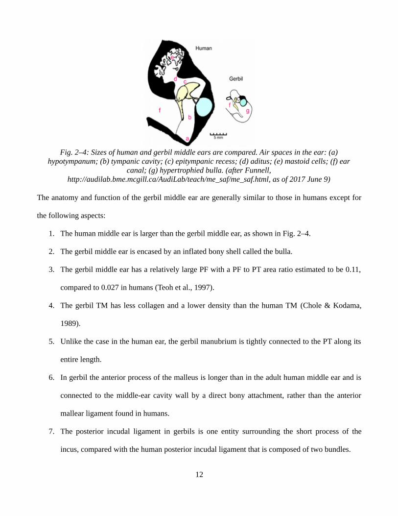
The anatomy and function of the gerbil middle ear are generally similar to those in humans except for

the following aspects:

1. The human middle ear is larger than the gerbil middle ear, as shown in Fig. 2–4.

2. The gerbil middle ear is encased by an inflated bony shell called the bulla.

3. The gerbil middle ear has a relatively large PF with a PF to PT area ratio estimated to be 0.11,

compared to 0.027 in humans (Teoh et al., 1997).

4. The gerbil TM has less collagen and a lower density than the human TM (Chole & Kodama,

1989).

5. Unlike the case in the human ear, the gerbil manubrium is tightly connected to the PT along its

entire length.

6. In gerbil the anterior process of the malleus is longer than in the adult human middle ear and is

connected to the middle-ear cavity wall by a direct bony attachment, rather than the anterior

mallear ligament found in humans.

7. The posterior incudal ligament in gerbils is one entity surrounding the short process of the

incus, compared with the human posterior incudal ligament that is composed of two bundles.

12

Fig. 2–4: Sizes of human and gerbil middle ears are compared. Air spaces in the ear: (a)hypotympanum; (b) tympanic cavity; (c) epitympanic recess; (d) aditus; (e) mastoid cells; (f) ear

canal; (g) hypertrophied bulla. (after Funnell,http://audilab.bme.mcgill.ca/AudiLab/teach/me_saf/me_saf.html, as of 2017 June 9)

Chapter 3: Literature review

3.1 IntroductionIn this chapter, we present a review of concepts and previous studies relevant to our research. In section

3.2, tympanometry is explained. In section 3.3, a review of the finite-element method and its

application in auditory research is presented. A review of previous experimental studies on the middle

ear is included in section 3.4.

3.2 TympanometryTympanometry is a promising clinical tool for evaluating the status of the middle ear in newborns. It

measures acoustical input admittance in the presence of a range of static pressures. In section 3.2.1, we

introduce the principles of tympanometry. We present the clinical applications of tympanometry in

section 3.2.2 and summarize the use of tympanometry in newborns in section 3.2.3.

3.2.1 Principles of tympanometry

Immittance is a term used to refer to both impedance Z and admittance Y. Impedance (measured in

ohms) is a measure of the opposition of a system to forces, and admittance (measured in mhos) is the

reciprocal of impedance. In acoustics, the admittance of a system is defined by

Y=U /P , (3–1)

where U and P are the volume velocity and the acoustical pressure, respectively, at the point where the

measurement is performed. Volume velocity is the volume of fluid (e.g. air) that passes through a unit

surface area per unit time.

The impedance is defined by

Z=1 /Y . (3–2)Admittance and impedance are complex numbers, which can be expressed either by magnitude and

phase or by real and imaginary parts. Admittance can be expressed as

13

Y=G+ jB (3–3)where G is the conductance, B is the susceptance and j=√−1 . The unit of acoustical admittance is the

mho (m3/Pa.s). In tympanometry, in addition to the acoustic stimulus, a pump generates quasi-static

pressures ranging generally between −400 and +400 daPa (−4 and +4 kPa), going from negative to

positive pressures or vice versa. (The unit usually used in clinical tympanometry for pressures is daPa

and 1 daPa=10 Pa.)

Fig. 3–1 is an illustration of a tympanometer. A hand-held probe is inserted into the ear canal and

forms a leak-free space from the probe tip to the TM. The probe is comprised of three components: a

small sound source , a microphone and a pump. The sound source delivers the acoustic stimulus to the

ear canal through a tube, and the pump generates varying quasi-static pressures within the sealed canal.

The microphone measures the sound pressure level at the probe-tip location. The voltage at the

microphone output is monitored to control the sound pressure in the ear canal. The voltage values are

then converted to an equivalent admittance value.

Fig. 3–1: Shematic diagram of a tympanometer (after Funnell,http://audilab.bme.mcgill.ca/AudiLab/teach/me_obj/me_obj009.html, as of 2017 August 18)

Tympanometry is widely used to assess middle-ear status. It was introduced into clinical practice

during the 1970s (Stach, 2008, p. 314) and its clinical use is established in adults. The acoustical

14

admittance is an indication of the amount of sound energy absorbed and reflected by the TM.

The middle ear can be thought of as a system composed of mechanical masses, springs and

dampers. The admittance of this system is frequency-dependent; it is stiffness-controlled at low

frequencies and mass-controlled at high frequencies. Damping plays an important role at mid to high

frequencies.

The goal of acoustical immittance measurement is to characterize the middle ear, but the probe tip

cannot be placed at the TM and is instead placed near the entrance of the ear canal. Consequently, the

admittance measured at the probe tip (Ya) (i.e., “a” for acoustical) is the sum of the admittance of the

ear-canal volume (Yec) and the admittance at the TM (Ytm). If we know Yec, we can thus calculate Ytm.

Terkildsen and Thomsen (1959) suggested that Yec can be measured independently when a large static

pressure (e.g., 200 daPa) is applied. At such a high pressure, the TM and the other middle-ear structures

are pushed almost to their limits and can no longer vibrate very much. Thus, all (or at least most) of the

energy of the probe tip is reflected at the surface of the eardrum, making Ya≈ Yec. In Fig. 3–3B, Ya is

equal to 1 mmho at 200 daPa. If the volume of the ear canal changes, Ya shifts higher or lower on the y

axis without altering the shape of the tympanogram. Several studies (e.g., Shanks & Lilly, 1981) have

shown that 200 daPa is not actually sufficient to drive the TM admittance to zero.

15

Fig. 3–2 Two methods of analyzing 226-Hz tympanograms. A: A qualitative analysis of tympanogramshape, designated as Type A B, or C (Strain & Fernandes, 2015). B: A quantitative analysis of

equivalent canal volume (Vea in cm3), acoustic admittance ( Ytm in mmho), tympanogram peak pressure(TPP in daPa), and tympanogram width (TW in daPa) (Adapted from:

https://www.slideshare.net/amirmah/topic5-49228595).

Acoustic admittance as a function of varying air pressure in the external ear canal for a specific

probe-tone frequency results in a graph called a “tympanogram”. Fig. 3–2 demonstrates two methods,

one qualitative and one quantitative, for analyzing tympanograms. The qualitative typing procedure

(Fig. 3–2A) was introduced by Jerger (1970) and is still deeply ingrained in clinical practice (Park,

2017). A normal tympanogram has a peak near 0 daPa and is asymmetric with higher admittance values

for positive pressure values than for negative values. The asymmetry is attributed to eardrum

movement, enlargement of the cartilaginous portion of the ear canal, movement of the probe tip,

residual middle-ear effects and viscoelasticity of soft tissues (Elner et al., 1971). Such a tympanogram

is designated as type A. Subcategories of type A are AS (i.e., “S” refers to a shallow notch in an

impedance tympanogram) for a small peak (low admittance) and type AD (i.e., “D” refers to a deep

notch in an impedance tympanogram) for a sharp peak (high admittance). Type AS tympanograms are

associated with otosclerosis and type AD are associated with ossicular discontinuity or atrophic scarring

of the eardrum (Shanks & Shohet, 2009). Type B tympanograms are flat and generally occur with

middle-ear effusion and eardrum perforation. Type C tympanograms are characterized by negative peak

16

pressures indicating negative pressures in the middle-ear cavity, characteristic of a malfunction of the

Eustachian tube. Differentiating among different types of tympanograms is very subjective. Feldman

(1976) criticized this coding procedure as it may cause confusion, and recommended a more

quantitative analysis of tympanometry with a focus on quantitative measures.

Fig. 3–3B shows how a tympanogram can be analyzed in terms of four numbers: acoustic

admittance magnitude Ytm (mmho), peak pressure TPP (daPa), width TW (daPa), and external ear canal

volume Vea (ml). These four numbers differ in their degrees of diagnostic relevance. Tympanometry can

also be analyzed in terms of the real part and the imaginary part of the acoustic admittance (i.e.,

conductance and susceptance). This has been used to study the W-notching of tympanograms in

response to high acoustic frequencies to evaluate mass-related pathologies of the middle ear (Vanhuyse

et al., 1975) .

3.2.2 Clinical applications of tympanometry

The first clinical application of clinical immittance measurement was in the 1940s, and it was starting

to be widely used in clinical practice during the 1970s. Early tympanometry devices only provided

qualitative and semi-quantitative measurements of middle-ear impedance. Quantitative measures were

later added, leading to the widespread use of tympanometry as a routine clinical procedure in

audiological examination for older children and adults. It is a well-established method for the

physiological assessment of the middle ear. Although there are only limited correlations between

tympanometry and specific middle-ear pathologies, it has often been used to estimate middle-ear

pressure, determine the presence or absence of fluid in the middle ear, and assess the condition of the

ossicular chain.

Tympanometry was initially performed at 226 Hz with no consideration as to the diagnostic value of

that particular frequency. This was mainly done for calibration reasons: at standard sea-level air

17

pressure, the compliance of 1 cc of air for a 226-Hz pure tone is equal to 1 mmho. Most diagnostic

immittance measurements on adults still use a 226-Hz probe tone because it has shown definitive

advantages for testing in adult middle ears (Roup et al., 1998). The frequency 226 Hz is below the

normal adult middle-ear resonance, which lies between 650 and 1400 Hz, so the effects of mass and

damping are minor. Normal 226-Hz tympanograms are single peaked, and as the probe frequency

increases tympanograms begin to display notches in a systematic way.

Multifrequency tympanometry (MFT) emerged in the 1970’s as a promising new method for

identification of middle-ear conditions. The use of multiple frequencies results in more information

(e.g., Alberti & Jerger, 1974; Colletti, 1975; Funasaka et al., 1984; Keefe & Levi, 1996; Shahnaz et al.,

2008), and MFT has been shown to improve the test sensitivity in some cases of conductive hearing

loss and outer/middle ear pathologies (e.g., Ferekidis et al., 1999; Shahnaz et al., 2008).

There are two methods of achieving MFT: sweep-pressure (Colletti, 1975) and sweep-frequency

(Funasaka et al., 1984) procedures. In the former method, a full course of quasi-static pressure variation

is performed, while the probe tone is held constant at a certain frequency, and the procedure is repeated

for multiple discrete frequencies. In sweep-frequency MFT, a wideband acoustic stimulus is introduced

to the ear canal in the presence of a sweeping quasi-static pressure. The acoustic stimulus can be a

sweep-frequency tone, also referred to as a chirp (Funasaka et al., 1984) , or a click (e.g., Keefe &

Simmons, 2003). The sound stimulus is repeated during the pressurization cycle (e.g., every 40 ms).

Within the duration of the acoustic stimulus, the quasi-static pressure changes are very small (e.g.,

0.48 daPa for a pressure course of –400 to +200 daPa at a rate of 50 daPa/s as in Therkildsen &

Gaihede (2005)). This leads to the assumption that the pressure remains constant within each chirp or

click.

MFT can be used to measure the resonance frequency of the middle-ear system. The resonance

frequency may be altered due to middle-ear disorders that affect the mass and stiffness of the middle

18

ear components. For instance, in the case of otosclerosis (i.e, a middle-ear disease caused by an

abonormal growth of bone that reduces the vibration of the ossicles), the stiffness of the middle ear

increases, resulting in an increase of the middle-ear resonance frequency. On the other hand, an

ossicular-chain disruption results in a decrease in the stiffness of the middle ear and consequently a

decrease in the middle-ear resonance frequency. It has been reported that MFT can detect otoclerosis

(Van Camp & Vogeleer, 1986).

Vanhuyse (1975) made a significant contribution to understanding how the tympanogram changes as

a function of frequency. At low frequencies (e.g., below 2 kHz), the acoustic pressure distribution is

approximately uniform in the ear canal and across the TM. At higher frequencies, however, the

interaction between the impedance of the ear canal and TM becomes complex, and the ear canal and

TM can no longer be considered as a parallel system. The complex behaviour of high-frequency

admittance tympanograms has limited their usefulness so far for the identification of middle-ear

pathologies. That is why multi-frequency probe tones are not used clinically as often as the 226 Hz

probe tone.

3.2.3 Tympanometry in newborns

Hearing is very critical for speech acquisition in children. Hearing loss can result in subsequent

behavioural, psychological and educational difficulties. Early screening for hearing loss is important so

it can be addressed in a timely manner. Neonatal hearing screening often uses an evoked otoascoustic

emissions (EOAE) test as the first step, to assess cochlear function. EOAE measures the sound

produced in the cochlea and is affected by any abnormalities in the sound transmission either forward

or in reverse through the middle ear. Acoustic brainstem response (ABR) tests are sometimes used as a

second step in neonatal hearing screening. ABR uses surface electrodes placed on the infant’s head to

measure the auditory nerve’s response to sound. Immittance measurements have been recommended

19

for inclusion in a battery of screening tests to identify any abnormality in an infant’s hearing (e.g.,

Calandruccio et al., 2006; Shahnaz et al., 2008). ABR and OAE results are believed to be most

effective when they are interpreted along with tympanometry measurements (e.g., McKinley et al.,

1997; Kilic et al., 2012).

It has been shown that 226-Hz tympanograms in infants below the age of 6 months are not as

reliable as in adults (e.g., Paradise, 1982; Holte et al., 1990). For instance, it is possible to obtain

normal 226-Hz tympanograms in infants even with confirmed middle-ear effusion (Meyer et al., 1997).

It is also possible to obtain abnormal-looking low-frequency pure-tone tympanograms in normal infant

ears (McLellan & Webb, 1957). The interpretation of tympanograms in infants is very different from

the case in adults. This is attributed to the anatomical differences (Fig. 3–3) in the developing newborn

ear (e.g., McLellan & Webb, 1957; Holte et al., 1991). The changes in the external and middle ear after

birth that could account for the acoustic alterations include:

• The newborn canal wall undergoes ossification.

• The sizes of the ear canal, middle-ear cavity and mastoid continue to change after birth.

• The relative orientation of the TM and the ear canal is different in newborns than in adults.

• The TM in infants is thicker than in adults, but less stiff.

• The tympanic ring is not fused in newborns.

• The density and the size of the ossicles change, and the mesenchyme, amniotic fluid and residual fluid clear out during the first hours and days after birth (Roberts et al., 1995) leading to a decrease in the overall mass of the middle ear.

• The ossicular joints tighten after birth.

20

Fig. 3–3. Comparison of the ear anatomy between newborns and adults (After Fowler EP Jr. (1947):Medicine of the ear, 2nd ed., T. Nelson, New York from

http://audilab.bmed.mcgill.ca/AudiLab/teach/me_saf/me_saf016.html, as of 2017 August 8)

It has been recognized that the external and middle ear systems can vary significantly in their

acoustic response properties over the first 2 years after birth (André et al., 2012). Higher-frequency

probe tones have been explored and displayed improved specificity and better correlation with

OAE/ABR screening. Through the use of either MFT or single high-frequency probe tones, it has been

concluded that high-frequency tympanometry can more accurately identify middle-ear effusion

(Marchant et al., 1986). Many studies have stated that the use of 1000-Hz probe tones is preferable to

the use of 226-Hz probe tones for infants (e.g., Kei et al., 2003; Wet et al., 2007; Glater, 2009; Kilic et

al., 2012).

Other studies have also tested the performance of MFT in infants. McKinley et al. (1997) measured

both multi-frequency tympanograms (at 226, 678 and 1000 Hz) and evoked otoacoustic emissions

(EOAE) in first-day neonates. They reported that there is no clear correlation between admittance

characteristics and EOAE results. Shahnaz et al. (2008) investigated MFT in 3-week-old infants and

adults. They found that at 1000 Hz, the admittance tympanograms had a single peak for 74% of infant

21

ears, while 78% of adult ears showed multiple-peak or irregular patterns. They also investigated MFT

in well babies and intensive-care-unit babies (with an average age of 3 weeks) at 9 frequencies (from

226 to 1000 Hz). They found that the tympanograms obtained at 1 kHz are more sensitive and specific

for presumably abnormal and normal middle-ear conditions, and that tympanometry at 1 kHz is a good

predictor of the presence or absence of transient EOAE’s.

3.3 Finite-element methodIn this section we discuss the finite-element (FE) method and some concepts that are important to the

generation of our FE model of the middle ear. A definition of the FE method and its basics are

summarized in section 3.3.1. Nonlinear and time-dependent models are defined in section 3.3.2.

Previous FE models of the middle-ear are reviewed in section 3.3.3.

3.3.1 Introduction

Continuum mechanics is concerned with the mechanical behaviour of solids and fluids on macroscopic

scales. Continuum mechanics applies fundamental physical laws to continua to derive partial

differential equations describing their behaviour. Information about the particular materials of the

continua is added through empirical constitutive laws.

The existing strategies to solve stress problems include analytical solutions. They can be derived

from the differential equations only for simple cases and rapidly become very complex for more

elaborate materials, geometries and loading conditions. In fact, exact analytical solution methods for

solving problems in deformable mechanics often don’t exist. Real engineering applications seldom

involve geometries or loading conditions exactly equivalent to those analyzed, so use of these methods

often involves some approximations.

Numerical methods are appropriate when no plausible idealization of the real problem can be

analyzed, or when greater accuracy is required than the idealization is expected to produce. By far the

22

most versatile and widely used numerical method is the FE method that dates back to the work of

McHenry, Hrenikoof and Newmark in the field of solid mechanics (e.g., Zienkiewicz et al., 1977). Here

we present a brief description of the method, but a more detailed overview can be found in standard FE

method textbooks (e.g., Dhatt et al., 2012).

A mesh of the geometry is built with a finite number of elements. An exact domain Ω is

approximated by the union Ωh of N non-overlapping elements Ωe (h) in such a way that:

Ωh=N∪

e=1Ωe(h) , lim

h→0(

N∪

e=1Ωe (h))=Ω (3–4)

where h reflects the size of the elements.

The sought-for solution is then approximated over each element by means of a function

approximation (usually a simple polynomial expansion) and is quantified in terms of values at discrete

points within the elements called the nodes. The discretization process establishes an algebraic system

of equations to approximate the continuous solution.

To develop the FE equations, we must first formulate the ‘strong form’ of the boundary-value

problem, which consists of the ordinary or partial differential equations together with the appropriate

boundary conditions. The strong form can be restated in an integral form called the ‘weak form’ which

can be proved to be equivalent to the strong form. The name weak form originates from the fact that

solutions have weaker continuity requirements than solutions of the strong form.

The FE strategy uses a Rayleigh-Ritz approximation in a piecewise manner on each finite element to

linearize the weak formulation for each element. Solving the resulting system of linear equations

provides the response of the system. The Rayleigh-Ritz approach considers a series of trial

approximation that satisfy the displacement boundary conditions in a point-wise fashion but not the

partial differential equations.

The FE method can be very accurate with certain assumptions on the behaviour of each element and

23

proper boundary conditions. The FE method can also be misleading and even dangerous without a good

knowledge of basic FE Method theory. In fact, a number of factors should be carefully considered to

ensure an adequate and accurate representation of reality:

1. Mesh convergence analysis: A systematic mesh convergence analysis should be performed.

Identifying an appropriate mesh size that yields accurate results at an acceptable computational

cost is essential. The finer the mesh is, the bigger the system of equation is, resulting in a high

computational cost.

1. Constitutive laws: Choosing the appropriate material properties to model the material behaviour

is important. For instance, modelling rubber behaviour using linear isotropic constitutive laws is

inadequate unless strains are small enough. The nature of the deformations of the material

determines how it should be modelled. There are different constitutive laws to model a wide

range of nonlinear behaviour. A priori information about the material properties is favoured

over simply adjusting model parameters to fit a set of experimental results.

2. Boundary conditions, loading conditions and constraints: The interactions among the

components of the system and the interaction of the system with the environment are usually

very complex. A simplification of these interactions in the FE model should still provide an

adequate representation of reality.

3. Model verification and validation: Model verification refers to the verification of the FE

computer code and the mathematical calculations. It may consist of comparing the same FE

model with different solvers. Model validation is the process of comparing the FE model

numerical results with experimental measurements.

There are a number of software packages for FE modelling, either commercial or free and open-

source. Commonly used commercial FE software includes ANSYS (www.ansys.com/) and ABAQUS

(www.3ds.com/products-services/simulia/products/abaqus/). Both include the three steps of modelling,

24

namely preprocessing (geometry and mesh generation, model creation), solving, and post-processing

(results visualization). Free and open-source software may include the three previously mentioned

components in one product or be designed for certain limited functions. For example, Salome-Meca (at

www.code-aster.org/) is open-source software that incorporates the three steps of modelling. On the

other hand, some software is used for geometry and mesh generation (e.g., Fie, Tr3 and Fad at

www.audilab.bme.mcgill.ca/sw/, PreView at www.febio.org/preview/, Gmsh at www.geuz.org/gmsh/).

Other software is used to implement new constitutive laws to model mechanical behaviour not

supported by the FE solver (e.g., nonlinear material representation using MFront at

https://tfel.sourceforge.net/). The latter can be used with commercial software when they do not support

a certain mechanical behaviour. There is software that solves the mathematical equations (e.g., FEBio

at https://febio.org/febio/, and Code_Aster at www.code-aster.org/). Finally, there is also software to

visualize the output (e.g., PostView at www.febio.org/postview/, ParaView at www.paraview.org/).

3.3.2 Nonlinear and time-dependent material models

Nonlinearities in FE models can be classified into four types: geometric nonlinearities that arise from

large deformations; material nonlinearities that stem from nonlinear material properties (e.g., nonlinear

elasticity); contact nonlinearities; and boundary-condition nonlinearities (e.g., pressure loads that

change orientation during deformation).

Some materials exhibit time-dependent behaviour when deforming; they possess a memory of past

events and can both store and dissipate energy. These materials have both elastic and viscous

characteristics and are referred to as viscoelastic materials. In this brief introduction, we will provide

descriptions of hyperelastic and viscoelastic behaviours. Detailed overviews of nonlinear and time-

dependent materials can be found in standard textbooks (e.g., Christensen, 2012; Belytschko et al.,

2013).

25

3.3.2.1 Finite-strain theory

For simulations with moderate to large deformation, an appropriate method is required to describe the

geometric configuration. Let us consider a small segment dX=(dX, dY, dZ) between two points M(X, Y,

Z) and P(X+dX, Y+dY, Z+dZ) in an initial configuration of a solid continuum domain. The segment is

transformed through Ф into a different segment dx=(dx, dy, dz) separating the two points M*(x ,y ,z)

and P*(x+dx, y+dy, z+dz) in the deformed configuration. According to this mapping, one can write the

following relationships:

d x=Φ(P)−Φ(M )=Φ(X+d X )−Φ(X) , (3–5)

which can be linearized through a Taylor’s series expansion up to first order as

d x=Φ(X)+ ∂Φ∂X

⋅d X−Φ(X )=∂Φ∂ X

⋅d X , (3–6)

which leads to the definition of the gradient tensor of the transformation at X:

F(X )=∂Φ∂X

=RU (3–7)

where F(X ) is a second-order tensor known as the deformation gradient, which linearly transforms

any infinitesimal vector in the undeformed configuration to another infinitesimal vector in the

deformed configuration of the body; R is the orthogonal rotation tensor and U is the right stretch tensor

(where the term “right” means it is to the right of the rotation tensor R). The deformation gradient

tensor is not zero for a rigid-body transformation, making it inappropriate to measure deformation of a

mechanical body. Instead, the right Cauchy-Green deformation tensor C is more appropriate and arises

from mapping the scalar product of two initial infinitesimal vectors. It is defined by

C=F T F . (3–8)

Note its symmetry. The difference between the initial and modified scalar products gives rise to the

Lagrangian finite-strain tensor E which is also symmetric and is defined by

E=12(C−I ) (3–9)

26

where I is the unity matrix. The Green-Lagrange strain tensor is a measure of deformation and for a

rigid-body transformation it is null. It is written as follows with respect to the displacement:

E=12(∂u∂ X

+(∂u∂ X

)T

+(∂u∂ X

)T∂u∂ X

) . (3–10)

The principal invariants of C are defined as follows:

I 1=tr (C )=λ12+λ2

2+λ3

2

I 2=12(I 1

2−tr (C2

))=λ12λ2

2+λ2

2λ32+λ1

2λ32

I 3=det(C )=J 2=λ1

2λ22λ3

2

(3–11)

where λ1 ,λ2 , and λ3 are called principle stretch ratios and are the eigenvalues of the deformation

gradient tensor F, and J is called the Jacobian and represents the volume change ratio. If the material is

incompressible, the volume change is negligible and J =1 .

3.3.2.2 Hyperelasticity

A hyperelastic material is a type of constitutive model defined in terms of a stored-energy function W

which depends on the deformation locally (e.g., W(C) and W(F)). A hyperelastic material is an elastic

material that exhibits nonlinear behaviour during large deformation. Unlike the case for linear elastic

materials, the strain-stress relationship is not linear. The strain-energy function is frame-indifferent due

to the symmetry of the Cauchy stress tensor, and the second Piola Kirchhoff stress S can be computed

as follows:

S=∂W∂E

=2∂W∂C

. (3–12)

Within the context of isothermal processes and isotropic materials, there exists a unique decoupled

representation of the stored-energy function into volumetric and isochoric (volume preserving) parts

(Simo & Taylor, 1985) as shown below:

W=W iso+W vol . (3–13)

A number of constitutive equations have been developed that are expressed in terms of either strain

27

invariants or principal stretch ratios, derived from a strain-energy function, such as the Neo-Hookean,

Mooney–Rivlin, Veronda-Westmann, Ogden, Yeoh and Arruda-Boyce models (e.g., Holzapfel, 2000).

Hyperelastic materials have been widely used to simulate large deformations in nearly

incomprehensible soft tissue such as skin, brain tissue, breast tissue, liver and TM (e.g., Qi et al., 2008).

3.3.2.3 Viscoelasticity

In addition to nonlinear elastic behaviour and large strains, soft biological tissues also exhibit

time-dependent stress results, creep, stress relaxation and hysteresis, which reflect

viscoelastic behaviour. Many viscoelastic models have been proposed in the literature and compared

(Reese & Govindjee, 1997; Simo & Hughes, 2006; Ciambella et al., 2010). Viscoelastic models can be

separated into three groups: linear viscoelastic models (LV) applicable in infinitesimal strain theory,

quasi-linear visco-hyperelastic (QLVH) models, and fully nonlinear visco-hyperelastic (NLVH)

models. The latter two are both applicable for finite deformations (Charlebois et al., 2013). LV and

QLVH models share the characteristic that the stress response is decoupled between time and strain. On

the other hand, in the case of the NLVH model, the nonlinear equation depends on both time and strain:

the deformation gradient has a multiplicative split into a viscous part and an elastic part. We will

present here only isotropic models, which refers to the invariance of the constitutive response of a

material under superposed rigid-body motions of the reference configuration. The condition of isotropy

places strong restrictions on the form of the response function. Furthermore, many nonlinear

approaches are beyond the scope of this thesis. The focus here will be on QLVH models. They are

single-integral mathematical models which are an outgrowth of linear viscoelasticity convolution

integrals and lead to an extended superposition principle that can be used to evaluate nonlinear

viscoelastic materials.

Let us consider a model that includes an elastic branch, composed of an elastic spring element, in

28

parallel with an arbitrary number of viscous branches, each composed of an elastic spring and a damper

in series. This provides a generalized relaxation and creep model. Fig. 3–4 shows an example of a

circuit model composed of one elastic branch and N viscous branches. For this model, the stress

response is defined by the relationship:

σ( t)=E0ε(t)−∑i=1

N

Eiαi (3–14)

where σ denotes the total stress applied on the system, ε denotes the total strain, αi is an internal

variable that represent the inelastic strain in dashpot i with viscosity ηi, E0 is the initial modulus, and

the Ei are the spring constants. The initial modulus E0, the relaxation time constants τ i and the

relaxation functions are defined

E0=E∞+∑i=1

N

Ei>0

τ i=ηi

Ei

, i=1,... ,N

G( t)=E∞+∑i=1

N

E iexp (−t /τ i)

. (3–15)

Fig. 3–4:Schematic of the Generalized Maxwell Model (Source:https://en.wikipedia.org/wiki/Generalized_Maxwell_model as of 2017 June 29)

This simple model can be extended to three-dimensional linear elasticity. In LV models, the stress is

linearly proportional to the strain history, and the stress tensor can be expressed in a closed form as a

29

convolution integral:

σ ( t)=dW vol

dJI +∫

−∞

t

g( t−s)dd(dev

∂W iso

∂ e)d s

dev .=.−13

tr (.) I(3–16)

where g(t), a sum of exponential time-dependent functions, represents the normalized relaxation

function (also defined as the Prony series):

g(t)=γ∞+∑i=1

N

γ i exp([−t / τi]) . (3–17)

Here γ∞ and γi represent the nondimensional Prony series coefficients constructed by the

relationship:

γ∞=E∞

E0

γi=E i

E0

, i=1,2,... , N

. (3–18)

The material parameters γ∞ , γi and τi are subject to these restrictions:

γ∞=1−∑i=1

N

γ i

0⩽γ∞<1γi⩾0τi>0

. (3–19)

When the strain is not infinitesimal, linear theory is inappropriate, and a nonlinear constitutive law has

to be considered. Fung (1993) introduced the QLVH model with the assumption that stress depends

linearly on the superposed time history of a related nonlinear response. The formulation is patterned

after linear viscoelasticity, and the stress response is, as in the linear theory, defined in the following

convolution representation:

S( t)=∫−∞

t

g (t−s )dd s

(Se(s))d s (3–20)

where Se represents the instantaneous second Piola-Kirchhoff stress tensor and may be thought of as

30

an equivalent elastic stress. The strain-energy function is split into a long-term equilibrium response W∞

and a nonequilibrium response Wk which represents the stored energy in the material that will relax

viscously in time:

W=W∞+∑i=1

N

W i . (3–21)

Each i=1,...,N represents a different relaxation mechanism in the material. The crucial idea is to use

internal variables to represent the nonequilibrium stresses associated with these mechanisms. Thus, the

stress response for a QLVH constitutive model is given by

S( t)=2dW∞

dC(t)+∑

i=1

N

Qi(t) (3–22)

where Qi(t ),u=1,2,... ,N , are internal variables governed by the evolution equations:

Qi(t )+1/ τ iQ

i(t)=

dd t

[2∂W i

∂C]

limt→∞

Qi(t)=0

(3–23)

These relations can be expressed in convolution form as

Qi( t )=∫

−∞

t

exp[−(t−s)/ τi]dd s

[2∂W i

∂C]d s . (3–24)

In addition to this stress convolution model for finite-deformation viscoelasticity, the multiplicative

decomposition model is very suitable for many materials undergoing large deformations or changes in

their properties under deformations. In these NLVH models, the deformation gradient is divided into an

elastic time-independent deformation gradient Fe and a viscous time-dependent deformation gradient

Fv:

F=F e F v

(3–25)

This hypothesis is combined with the assumption of a viscoelastic potential to give a model similar to

associative elasto-plasticity (Govindjee & Reese, 1997). The energetic contribution of each mechanism

is assumed to depend on F ie through C i

e=[F i

e]T F i

e such that the overall strain energy of the material

31

can be expressed as:

W (C ,F iv)=W ∞(C )+∑

i=1

N

W i(C ie) . (3–26)

Note that W k depends on C ie rather than C as one would expect from a physical point of view since

the “elastic” deformation associated with each mechanism should not be part of the total deformation

of the material but only the driving force. In this model, the stress is also decomposed into an

equilibrium and a nonequilibrium contribution:

S=2d W ∞

dC+∑

i=1

N

2(F iv)−1 ∂W i

∂C ie (Fi

v)−T . (3–27)

The evolution equations for the internal viscous part of the deformation must satisfy the following

dissipation inequality for each relaxation mechanism independent of the others:

∂W i

∂F iv :(Fi

v)⩾0 (i=0,. .., N ) (3–28)

The elastic behaviour of the response is specified using the hyperelastic material model while the

viscous behaviour has different forms depending on the creep law chosen. NLVH models can predict

complex behaviour of materials. Unlike LV and QLVH models, they can be shown to always satisfy the

Second Law of Thermodynamics. Furthermore, they provide evolution equations that are valid far from

elastic equilibrium, and thus are not restricted to strain states near the elastic equilibrium.

3.3.2.4 Viscoelasticity and nonlinearity in the middle ear

The TM is a complex structure composed of multiple layers (section 2.3.1). It is also an

inhomogeneous structure with anisotropy in the radial, circumferential and through-thickness

directions.

In vitro measurements of the mechanical properties of the TM have been reported in the literature.

von Békésy (1960) estimated the Young’s modulus of the human TM to be 20 MPa using bending tests

32

on dissected human TM strips. Kirkae (1960) measured the Young’s modulus to be 40 MPa based on a

longitudinal dynamic test on strips of fresh human TM. Decraemer et al. (1980) reported results for a

uniaxial tension test of strips of human TM and proposed nonlinear elastic and nonlinear viscoelastic

structural models. At the large strains, a Young’s modulus of 23 MPa was found.

Fay et al. (2005) applied three different methods to estimate the elastic properties of the TM. First, a

constitutive model was used to estimate the properties of the cat TM based on known stiffness values of

collagen and on observed fibre densities. Second, both bending and tensile loading tests for the TM

were reinterpreted using composite laminate theory to find the range of elastic modulus values for the

fibre layers. Third, the dynamic displacement of the TM was measured as a function of frequency. A

wave-number vs. frequency relationship was determined which represents a fundamental property of

the TM’s mechanical structure. From these three different methods, they reported a range of elastic

moduli for the human TM ranging between 0.1 GPa and 0.3 GPa, which is significantly higher than

values reported elsewhere. The high Young’s modulus in Fay’s study is, at least in part, because they

use a much smaller thickness for their specimens, corresponding to only the fibre layers. These

variations in measurements between different groups may also be due to the fact that the Young’s

modulus of the TM is frequency dependent, and all the previous measurements were performed at

different frequencies.

In normal hearing the middle ear behaves linearly, but it becomes nonlinear in response to high

sound pressures, to blast and explosions, and to the large quasi-static pressures involved in large

changes of altitude and in clinical tympanometry. In these scenarios, soft tissue in the middle-ear (e.g.,

the TM and the ligaments) shows typically time-dependent behaviour, and also elastic deformations

that can reach large values.

In the middle-ear, the TM functions over a broad frequency range. By measuring surface

displacement of the TM as a function of frequency as when it is acoustically driven, Fay et al. (2005)

33

demonstrated that, like many other soft biological tissues, the TM exhibits viscoelastic behaviour upon

deformation. Different formulations have been introduced to derive the constitutive equations of the

TM (e.g., Motallebzadeh et al., 2013).

Fung (1993) discussed the viscoelasticity of soft tissue in the light of two important features of the

loading and unloading curves: hysteresis and preconditioning. In response to cyclic loading, the stress-

strain curve in the unloading process is different from that in the loading process. This dynamic

phenomenon is called hysteresis and is often approximately independent of frequency over a wide

range of frequencies (Fung, 2013, p. 289). Successive loading and unloading changes the stress-strain

curves from cycle to cycle until it reaches a steady state after a few cycles, and this is referred to as

preconditioning.

Chang et al. (2007) reported a series of mechanical measurements on strips of the human TM to

characterize its viscoelastic properties. They performed uniaxial tensile, stress relaxation, and failure

tests, on specimens taken from human cadaver eardrums, under quasi-static loading conditions. They

cut 11 rectangular strips from the posterior side of the eardrum, clamped them at both ends and

mounted them in the material-testing system. The maximum strain was 15%. Curves of stress vs.

stretch ratio for one eardrum specimen are shown in Fig. 3–5. The preconditioning is observed in

Fig. 3–5a with curves decreasing during repeated loading-unloading curves until they reach a steady

state after the third cycle. The hysteresis phenomenon was also observed, with the unloading curve

being lower than the loading curve. Based on these stress-stretch data, Cheng et al. identified Ogden

model parameters to model the nonlinear elastic properties of the TM for different stress ranges. The

stress-relaxation behaviour of the TM for 9 specimens was also reported. The stress decreases with

time and reaches a relatively stable level after 120 s. At 1 s, 10% of the stress is relaxed; at 5 s, 20% of

the stress is relaxed; at 50 s, 35% of the stress is relaxed. The viscoelastic properties of the TM were

described but not modelled.

34

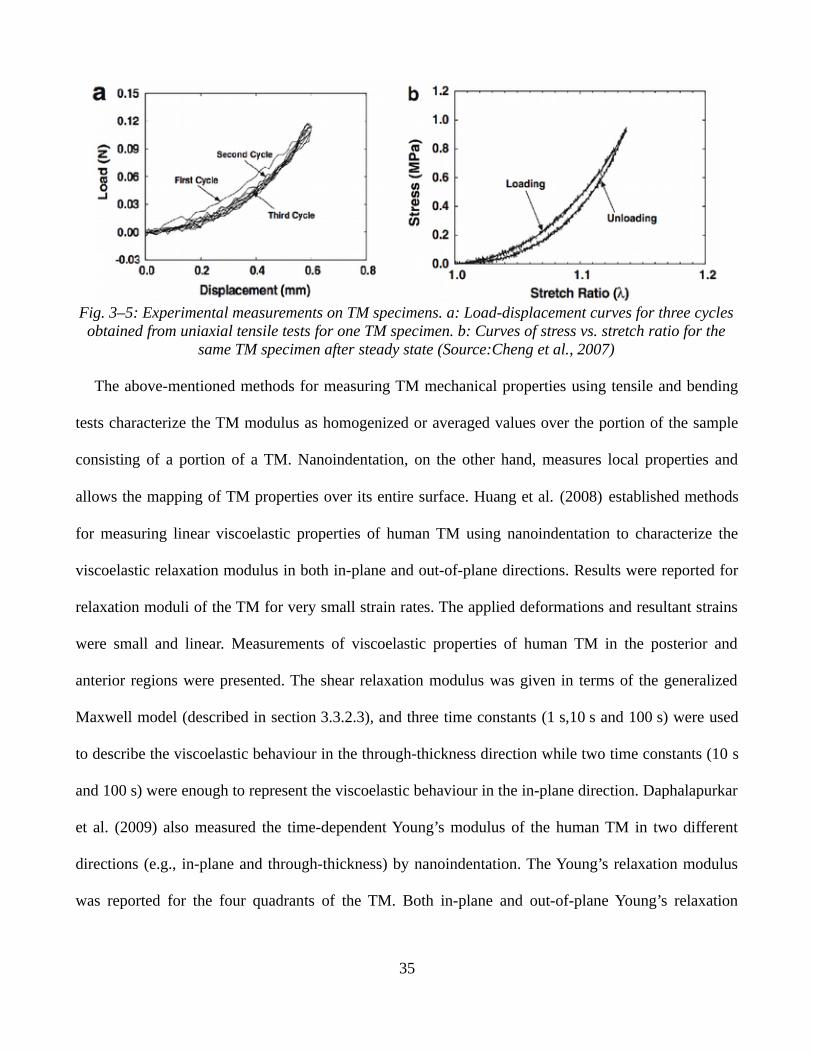
Fig. 3–5: Experimental measurements on TM specimens. a: Load-displacement curves for three cyclesobtained from uniaxial tensile tests for one TM specimen. b: Curves of stress vs. stretch ratio for the

same TM specimen after steady state (Source:Cheng et al., 2007)

The above-mentioned methods for measuring TM mechanical properties using tensile and bending

tests characterize the TM modulus as homogenized or averaged values over the portion of the sample

consisting of a portion of a TM. Nanoindentation, on the other hand, measures local properties and

allows the mapping of TM properties over its entire surface. Huang et al. (2008) established methods

for measuring linear viscoelastic properties of human TM using nanoindentation to characterize the

viscoelastic relaxation modulus in both in-plane and out-of-plane directions. Results were reported for

relaxation moduli of the TM for very small strain rates. The applied deformations and resultant strains

were small and linear. Measurements of viscoelastic properties of human TM in the posterior and

anterior regions were presented. The shear relaxation modulus was given in terms of the generalized

Maxwell model (described in section 3.3.2.3), and three time constants (1 s,10 s and 100 s) were used

to describe the viscoelastic behaviour in the through-thickness direction while two time constants (10 s

and 100 s) were enough to represent the viscoelastic behaviour in the in-plane direction. Daphalapurkar

et al. (2009) also measured the time-dependent Young’s modulus of the human TM in two different

directions (e.g., in-plane and through-thickness) by nanoindentation. The Young’s relaxation modulus

was reported for the four quadrants of the TM. Both in-plane and out-of-plane Young’s relaxation

35

moduli exhibited pronounced viscoelastic effects. The in-plane steady-state Young’s relaxation

modulus did not show much variation across the four quadrants of each TM. The values obtained, 25.7

to 37.8 MPa (in-plane) and 2 to 15 Mpa (out-of-plane) are close to the values (40 MPa) reported by

Békésy (1960), Kirikae (1960) and Decraemer et al. (1980) the value (20 MPa) reported by von Békésy

(1960). In general, the out-of-plane Young’s relaxation modulus is considerably lower than the in-plane

modulus. On average, the out-of-plane relaxation Young’s modulus decreased by 50% from 1 s to

100 s. At the steady-state, the out-of-plane Young’s relaxation modulus varied considerably, from

2 MPa to 15 MPa, over the TM surface.

In the experiments described above, the properties of the TM were measured at very low strain

rates. Luo et al. (2009a, 2009b) used a split-Hopkinson pressure bar to measure the strain-rate-

dependent behaviour of the normal and diseased human TM at higher strain rates, from 300 to 2000 s−1,

in both the radial and circumferential directions. They found little difference between the Young’s

moduli in the radial (45.3-58.9 Mpa) and circumferential (34.1-56.8 MPa) directions, indicating an

isotropic behaviour even at high stain rates. At higher strain rates (1000-2000 s-1), the reported stress-

strain curves are linear except in the vicinity of failure strains, indicating nearly linear behaviour.

Furthermore, they observed an increase in the Young’s modulus with increasing strain rate, indicating

that the viscoelastic behaviour of the TM is dependent on strain rate.

Zhang and Gan (2010) conducted dynamic tests on the human TM up to 8000 Hz using a laser

Doppler vibrometer. The complex modulus was obtained by fitting the experimental measurements

using a FE model. In a later study, Zhang and Gan (2013) extended their results to higher than previous

quasi-static frequencies using frequency-temperature superposition (FTS). The basic theory of this

empirical method considers the viscoelastic behaviour of some materials as a function of two principle

variables: frequency and temperature (e.g., Ferry, 1980; Landel & Nielsen, 1993). The effects of

temperature changes on the viscoelastic properties of the material are assumed to be equivalent to those

36

of frequency changes. Their measurements were conducted at different temperatures in the frequency

range 1 to 40 Hz and extended to at about 7840 Hz using the FTS principle. The complex modulus of

the TM was found to generally increase with frequency. The largest slopes were observed below 10 Hz

and between 1000 and 3800 Hz. The change in slope at these frequencies relates to two time constants

used to fit the experimental data, with mean values of 5.14 ms and 78.6 μs. The mean storage and loss

moduli found in this study were lower than those found in the previous studies by Luo et al. (2009a,

2009b) and showed lower slopes as functions of frequency. Possible causes identified by Zhang and

Gan for these differences include cross-subject variability, the physiological condition of the TM and

its moisture level, or perhaps inadequacy of the FTS principle.

The measurements discussed above were all done on the human TM. Our study focuses on the gerbil

TM and measurements for this species are very limited. Aernouts and Dirckx (2012) studied the

mechanical behaviour of the gerbil TM under both quasi-static and dynamic loading conditions through

in situ indentation. The frequency-dependent Young’s modulus of each specimen was then estimated by

an inverse analysis. They reported Young’s moduli between 71 and 106 MPa at 0.2 Hz indentation

frequency.

Few measurements have been made of the material properties of the gerbil PF. The PF is a

continuation of the external ear canal skin (Lim, 1968), so its material properties may be close to those

of skin. Agache et al. (1980) estimated the Young’s modulus of the human forearm skin in vivo to be

0.42 MPa in their younger subjects and 0.85 MPa in subjects more than 30 years old. Geerligs et al.

(2011) performed in vitro indentation measurements on human abdominal skin and estimated the

Young’s modulus of the skin to be between 1 and 2 MPa. Due to the relatively simple geometry of the

PF, its behaviour can be approximated by that of a circular disk. Such numerical models have been used

in attempts to infer its material properties from experimentally measured large quasi-static

deformations but the estimated Veronda-Westmann parameters were inconsistent (Decraemer et al.,

37

2010; Aernouts and Dircks, 2011).

Similar to the TM, ligaments also exhibit nonlinear viscoelastic behaviour. For example,

Bonifasi-Lista et al. (2005) and Vena et al. (2006) found that human medial collateral ligaments exhibit

a clear nonlinear viscoelastic response. They found that the creep rate depends on the applied stress and

that the relaxation rate depends on the applied stretch. The stretch-dependent and time-dependent

behaviour of some ligaments in the middle ear has been investigated experimentally. Cheng and Gan

(2008) reported the mechanical properties of the anterior mallear ligament (AML) through uniaxial

tensile, stress-relaxation and failure tests. A nonlinear hyperelastic model was used to describe the

nonlinear behaviour of the AML. Unlike the isotropic model for the TM (Cheng et al., 2007), local

responses of fibres in the middle portion of the AML were used to describe the mechanical properties

of the ligament. The transverse effects of fibres were accounted for in the Ogden model by an

I4- reinforced term in the equation that corresponds to the square of material stretch in the fibre

direction. It was concluded that the stress distribution in the AML is much more complicated and

requires a more accurate description of its microstructure. The stress relaxation curve showed a stable

stress after 120 s. The material behaviour of fibrous soft tissues in general presumably depends on fibre

properties, matrix properties, fibre-matrix interactions and fibre-fibre interactions. Thus, multiaxial

tests (e.g., shear, transverse and longitudinal directions) are required to fully characterize the three-

dimensional material behaviour of ligaments in the middle ear. To the best of our knowledge, these

types of experiments on middle-ear ligaments are nonexistent.

3.3.3 Finite-element models of the ear

The first mathematical models of the middle ear included lumped-parameter models where each

middle-ear structure is lumped as an equivalent electrical circuit element (e.g., Zwislocki, 1957). In

these models, variables are only dependent on time and not on space. To address this issue, analytical

38

(Wada & Kobayashi, 1990) or semi-analytical models (Rabbitt & Holmes, 1986) were formulated.

However, these simplified models of the middle ear do not actually capture its complex 3D geometry

containing many interconnected, highly irregular, asymmetrical and non-uniform parts. On the other

hand, the FE method offers the possibility of modelling such a complex system and obtaining a

quantitative understanding of its function. In FE models, dependent variables are functions of both time

and spatial coordinates and can be connected to physiological characteristics of the middle-ear

structures. Here, only a brief review of previous FE models of the middle ear is provided. For a more

complete review of different approaches to modelling the middle ear, refer to Funnell et al. (2012).

Funnell and Laszlo (1978) presented the first FE model of the middle ear and investigated the low-

frequency behaviour of the cat TM within the range of linear vibration amplitudes. To represent the

three-dimensional curved conical shape of the TM, the curvature was represented by circular arcs. A

fixed axis of rotation running from the anterior mallear process to the posterior incudal process was

assumed, and stiff triangular elements connected the axis to the manubrium. The combined ossicular

and cochlear load was represented at the axis of rotation by a frequency-independent rotational

stiffness. Funnell (1983) extended this model to higher frequencies. The dynamic response of the

model to a uniform sound pressure was analyzed, and natural frequencies and mode shapes were

measured. Results from the model were qualitatively similar to the experimental observations of

Khanna and Tonndorf (1972) obtained in cat by time-averaged laser holography. Funnell et al. (1987)

added consideration of the inertial and damping effects in the cat TM model. The damping of the

system was represented by mass-proportional Rayleigh damping. Numerical results from the FE model

agreed quite well with laser interferometric point measurements on the cat TM (Decraemer et al.,

1989).

Lesser and Williams (1988) and Williams and Lesser (1990) presented linear dynamic FE models of

the human TM and ossicles in 2-D. However, it was known from previous studies that 3-D geometry

39

has an important effect on the behaviour of the middle ear. Wada et al. (1992) made the first 3-D FE

model of the human middle ear. It was a linear dynamic model that included the TM and ossicles.

Vibration patterns of the eardrum and ossicles were in agreement with the experimental results of

Khanna and Tonndorf (1972).

The mechanical behaviour of the eardrum depends heavily on its shape, so accurate geometric

modelling techniques for reconstructing the TM (and also other structures of the middle ear) are

essential for a good FE model. Funnell and Decraemer (1996) used phase-shift moiré topography to

accurately measure the shape of the cat TM and incorporated that shape in their FE model. They used

large static pressures to facilitate the determination of the boundaries of PF, PT and manubrium.

Prendergast et al. (1999) used nuclear magnetic resonance (NMR) spectroscopy images (of very low

resolution) to reconstruct the outer-ear and middle-ear geometry. Van Wijhe et al. (2000) segmented the

middle ear of the moustached bat from a magnetic-resonance microscopy (MRM) data set. Daniel et al.

(2001) used the moiré shape measurements for the TM shape in a FE model of the human middle-ear.

In Daniel et al. (2001) the ossicles and ligaments were reconstructed from histological sections and

high-resolution MRM data. Sun et al. (2002) used histological sections to reconstruct the TM geometry

where the distinction between PF and PT can be hard to detect. Decraemer et al. (2003) used

microscale X-ray computed tomography (μCT) imaging data to reconstruct the ossicle and TM

geometries. MRM and μCT imaging techniques allow the orientation and geometry of the TM to be

observed clearly, but cannot produce a detailed thickness distribution of the TM. Kuypers et al. (2005,

2006) used confocal microscopy and Van der Jeught et al. (2013) used optical coherence tomography

for full-field high-resolution thickness distribution maps and shape data of the TM. , For a thorough

review of image-segmentation methods used for 3-D reconstruction of the ear, see Ferreira et al.

(2014).

In FE models of the middle ear, a variety of constitutive models have been applied to different

40

components based on their mechanical behaviours. The simplest constitutive model is linear isotropic

elasticity, which can only simulate the behaviour of the middle ear in response to low pressures (e.g.

acoustic stimuli in the range of normal hearing). Funnell et al. (1987) modelled the TM by a single

layer of isotropic material, and Wada et al. (1992) modelled the ossicles as isotropic elastic materials.

Maftoon et al. (2015) developed a FE model of the gerbil middle ear with isotropic elastic properties

for the TM, the ossicles and the joints.

Orthotropic elastic models have also been applied to the TM to account for the orientation of

collagen fibres in the radial and circumferential directions (e.g., Gan et al., 2006; Wang et al., 2007).

Multilayered models of the TM have also been developed to consider the different layers of the TM

(e.g., Fay et al., 2006; Tuck-Lee et al., 2008).

Viscous and nonlinear behaviour of the TM has also been taken into account in some FE models of

the middle ear or its components. Ladak et al. (2006) modelled nonlinear deformations of the cat TM

by considering only the geometric nonlinearity. The effects of large static pressures within the range of

pressures used in clinical tympanometry were investigated. Their simulation results agreed with their

experimental shape and displacement patterns measured using phase-shift shadow moiré topography

(Ladak et al., 2004). They found that the location of the maximum displacement changes when the

pressures are varied, and concluded that geometric nonlinearity of the TM must be considered at high

pressures. However, material nonlinearity may become more important at high pressures. Qi et al.

(2006) modelled the dynamic response of the newborn ear canal while including both geometric and

material nonlinearities using a nonlinear hyperelastic constitutive law. They later used the same method

to model the newborn middle ear (Qi et al., 2008). Wang et al. (2007) studied middle-ear pressure

effects on the static and dynamic behaviour of the adult human ear. The static behaviour of the human

middle ear under various air pressures was investigated using a hyperelastic model. The static

deformation field then provided nodal displacements of the TM and middle-ear ligaments that were

41

used to update the model mesh for dynamic analysis. The latter was linear with material properties that

were adjusted for different stress ranges. The TM and stapes-footplate vibrations under various middle-

ear pressures were reported from the dynamic analysis. They concluded that reductions of the TM and

footplate vibration magnitudes under positive middle-ear pressures were mainly caused by nonlinear

material properties, but that the reductions under negative pressures were caused by both the geometric

and material nonlinearities. Rather than using true nonlinear material properties, Homma et al. (2010)

modelled the effects of large static pressures by empirically altering the linear material properties for

the different pressures. In a quasi-static model, Motallebzadeh et al. (2013) combined modelling of the

nonlinear and viscoelastic effects of strips of the TM for the first time. Their model could reproduce

both the relaxation and hysteresis curves of Cheng et al. (2007), which was “an important step toward

understanding the viscoelastic phenomena of the eardrum under conditions that are comparable to those

involved in tympanometry”.

In early FE models, the cochlear damping was not modelled explicitly and its effect was included in

the damping of the TM and ossicles (e.g., Funnell et al., 1987; Ladak & Funnell, 1996). Koike et al.

(2002) represented the cochlear damping in their middle-ear models by one dashpot connected to the

footplate of the stapes, based on experimental observations that the cochlear impedance is primarily

damping. Sun et al. (2002) modelled the cochlear load with 49 spring-dashpot elements oriented in the

direction normal to the footplate plane. Fluid models of the cochlea have also been incorporated in FE

models (e.g., Kim et al., 2011).

Although most middle-ear FE models have been developed for human, strong validation of FE

models requires data that can only collected, or can be collected with a higher quality, in experimental

animals. There have been some models for non-human middle ears. Models for the cat middle ear were

at one time extensively developed (e.g., Funnell & Laszlo, 1978; Funnell et al., 1987; Tuck-Lee et al.,

2008). Aernouts et al. (2010) created a FE model for the rabbit, and Ghadarghadar et al. (2013)

42

published a model for the rat. The gerbil is currently perhaps the most popular species for experimental

middle-ear research, and models of the gerbil middle ear have been developed (e.g., Funnell et al.,

2000; Elkhouri et al., 2006; Buytaert et al., 2011; Maftoon et al., 2015).

Daniel et al. (2001) discussed the clinical applications of FE modelling of the human middle ear. FE

models have been applied to study middle-ear pathologies (e.g., Dai et al., 2007; Gan & Wang, 2007),

middle-ear prostheses (e.g., Williams et al., 1995), middle-ear surgical repair procedures (e.g., Lee et

al., 2006), ear protection systems (e.g., James, 2006), and clinical tests (e.g., Wang et al., 2007;

Motallebzadeh et al., 2017).

3.4 Experimental measurements A variety of experimental measurement techniques have been used to study middle-ear mechanics both

post mortem and in vivo and in different species. Our research focuses on the response of the gerbil TM

to sound stimuli and static pressures. A review of previous studies pertinent to our research is presented

in this section. A review of human studies and other non-gerbil studies is presented in section 3.4.1.

Then, a review of experimental studies conducted on the gerbil middle ear using only sound stimuli is

presented in section 3.4.2. Studies that include quasi-static pressures only are highlighted in section

3.4.3. A review of studies involving both sound stimuli and quasi-static pressures is included in

section 3.4.4.

3.4.1 Measurements of non-gerbil tympanic-membrane vibrations

Early experimental measurements of TM vibrations were reviewed by Funnell and Laszlo (1982). The

review includes work as far back as 1874. Here, we only discuss some of the key studies mentioned in

the review and present studies that were done after the publication of that article.

After non-electronic observations by Kessel (1874) and Dahmann (1929), von Békésy (1941) used a

capacitive probe to measure TM vibration. He described the TM motion as a rotation of a stiff surface

43

about an axis superior to the TM at low frequencies (up to 2 kHz), and concluded that, because of the

rotation, the maximum vibration magnitude occurs inferior to the manubrium. He also qualitatively

described the motion of the TM for frequencies above 2.4 kHz, reporting that the conical shape of the

TM becomes less stiff and that the manubrium lags behind the PT portions near the manubrium.

Manley and Johnstone (1974) measured the velocity and displacement at various locations on the

guinea-pig TM over a broad range of frequencies (up to 25 kHz) using the Mössbauer technique with a

very small gamma-ray source. Since then, optical interferometric techniques have become very popular

and the primary means of investigating TM vibration patterns. Tonndorf and Khanna (1972) used time-

averaged laser holography to visualize and quantify the vibration patterns of the TM in cat and in

cadaveric human ears. They observed iso-amplitude contours on the vibrating TM. They showed that

even at low frequencies the TM does not move as a stiff surface as von Békésy described. They

identified regions of higher displacement magnitudes in the posterior and anterior regions of the PT,

with a maximum on the posterior side. This pattern remained almost the same up to about 2 kHz. At

about 3 kHz, the vibration patterns appeared to break up and became much more complex as the

frequency increased. Funnell and Laszlo (1978) discussed possible causes of the discrepancy between

von Békésy’s observations and those of Tonndorf and Khanna. Decraemer et al. (1989) utilized a

homodyne laser interferometer and reported phase and magnitude for a wide frequency range (130 Hz

to 20 kHz) for a few points on the cat PT and manubrium, using reflective objects to increase the

signal-to-noise ratio. They observed that up to 1 kHz all points on the PT moved almost in phase, but

beyond that frequency the phase differences increased and for frequencies above 5 kHz each point

moved very differently. Time-averaged holographic techniques provide full-field observations of

sound-induced motions of the TM surface, but point-by-point laser interferometry provides more

precise magnitude and phase information. This technique also has a finer frequency resolution.

Tonndorf and Khanna (1968) developed a laser interferometer and studied vibrations in the cat at the

44

umbo. Buunen and Vlaming (1981) used a laser Doppler vibrometer (LDV) to measure the magnitude

and phase of the umbo vibrations in the cat. LDV measures vibration velocity over a broad range of

frequencies by computing the Doppler frequency shift of the light that is being scattered. Konrádsson et

al. (1987) studied vibrations of the human TM in vitro using a scanning LDV and presented data at 578,

3107 and 3113 Hz. The observations were consistent with earlier studies. Decraemer et al. (1989) used

an improved interferometer that did not require reflective objects, allowing them to obtain vibration

measurements with higher spatial resolution. They concluded that the motion “looks more like a

traveling wave than like a standing wave”.

Akache et al. (2007) in our lab performed post mortem LDV measurements on the rat TM. They

used microbeads to enhance the signal quality and reported displacement magnitudes in the frequency

range of 1 to 10 kHz. They observed no break-up in the simple TM vibration pattern up to 10 kHz,

which may have been due to drying of the middle-ear structures in their post mortem measurements.

In a series of in vivo studies in healthy and pathological human ears, the potential clinical diagnostic

utility of LDV measurements at the umbo has been evaluated. Huber et al. (2001) used scanning LDV

on TMs from subjects with normal hearing and from subjects with conductive or sensorineural hearing

loss. Based on the umbo response, they suggested that scanning LDV can detect conductive hearing

loss and can distinguish among a few middle-ear conditions. Rosowski et al. (2008) demonstrated that

LDV can be used for diagnosis and differentiation of various ossicular disorders through a series of

measurements near the umbo in live human subjects and patients.

Recent advances in software and hardware have enabled the development of modern TM

holographic measurements and enabled measuring at higher frequencies. Rosowski et al. (2009)

performed computer-assisted time-averaged holographic measurements in ears of cadaveric chinchillas,

cats and humans and in a live chinchilla. Based on their observations, they classified the TM motions

into three regimes. At the lowest frequencies, the displacement patterns are fairly simple, with one to

45

three displacement maxima. At 4 kHz in the cat and human and 1 kHz in the chinchilla, they observed

more complex patterns composed of areas of concentric rings of high-magnitude motions separated by

rings of low-magnitude motions. This regime was named ‘complex pattern’ and had been described in

previous studies (e.g., Khanna & Tonndorf, 1972) as the breakup of the simple low-frequency motion.

At higher frequencies, above 8 kHz in the cat and human and above 4 kHz in the chinchilla, they

observed another regime of vibration pattern that they named ‘ordered pattern’. In this regime, a large

number of displacement maxima are arranged in an orderly fashion in the radial and circumferential

directions, and they alternate with displacement minima. The same group later integrated stroboscopy

in their holographic setup to measure phase of the motion as well Cheng et al. (2010). They concluded

that the TM motion is a combination of standing waves and “some smaller traveling-wave like

components”. Later, the group used the same setup with two laser wavelengths (Rosowski et al., 2013)

to also compute the 3D-shape of the chinchilla TM. The in-plane TM motions were found to be

significantly smaller in magnitude than the out-of-plane motions, which is consistent with the thin-shell

theory of mechanics.

3.4.2 Unpressurized vibration measurements in gerbils

Some groups (e.g., Ravicz et al., 1992; Ravicz & Rosowski, 1997; Teoh et al., 1997) have investigated

the input admittance of the gerbil TM in response to acoustic stimuli at different frequencies as an

indirect measure of middle-ear vibration responses to sound. Although admittance is easy to measure, it

does not provide information about the spatial vibration patterns of the TM, which are important to

gain a better understanding of middle-ear mechanics and for diagnostic purposes.

Studies of the vibration patterns of the gerbil TM in response to sound pressure are very scarce. De

La Rochefoucauld and Olson (2010) measured the vibration of the gerbil TM at a few points on the PT

near the umbo as well as along the manubrium. Aside from these measurements, only our group has

46

published studies that investigate the vibration pattern of the gerbil TM. Ellaham et al. (2007) reported

LDV measurements at multiple points in five post mortem gerbils. Magnitudes of displacement were

measured at points along the manubrium as well as on the PT over a frequency range from 0.15 to

10 kHz. The study provided a detailed longitudinal tracking of the effect of the drying of middle-ear

structures on vibration measurements. Nambiar (2010) performed post mortem studies similar to those

of Ellaham et al. but with much better hydration of the middle-ear structures, to try to avoid the post

mortem effects of drying. Matoon et al. (2012) reported our first in vivo TM vibration patterns and He

(2012) devised an experimental approach to widely expose the TM more widely. In a more recent study

in our group, Maftoon et al. (2013, 2014) used LDV to perform in vivo vibration measurements of the

gerbil TM at several points on the PT, along the manubrium and on the PF. The response of the TM to

audio-frequency chirps in the ear canal was reported. Data were presented for two PF conditions:

naturally flat, and retracted into the middle-ear cavity. At low frequencies, they reported a minimum

and a shallow maximum in the magnitude responses of the manubrium caused by resonance of the PF

when in its flat condition. On the other hand, a retracted PF resulted in reduced displacement

magnitudes and no effects on the responses of the manubrium and PT. They reported that the break-up

of the simple low-frequency pattern occurs between 1.8 and 2.8 kHz for all PT points. At higher

frequencies, they observed more complex vibration patterns on the PT and a roll-off of the magnitude

responses on the manubrium, including the umbo, with substantial irregularities.

3.4.3 Static pressure deformations

Apart from acoustic pressures, the middle ear is also subject to very slow quasi-static pressures due to

changes in ambient pressures and to mechanisms of gas exchange (Dirckx et al., 2001). Changes in

static pressure are also involved in tympanometry, a useful clinical diagnostic tool for assessing the

condition of the middle ear. Static pressures change the stiffness of the middle-ear system and alter its

47

acoustic transfer function.

Quasi-static deformation of the gerbil TM under static pressure has been measured in several studies

by the group of Decraemer and Dirckx in Antwerp. To start with, Von Unge et al. (1993) studied gerbil

PT deformations under static pressure using real-time differential moiré topography. Their

measurements showed hysteresis between the loading and unloading cycles and convergence to a

preconditioned state after the second cycle. Two areas of maximum magnitude were observed, one on

the anterior side and one on the posterior side of the PT, at approximately the same level. The locations

of the areas remained constant as the pressure increased. Dirckx et al. (1997, 1998) studied gerbil PF

deformation under positive and negative static pressures varying from −2 kPa to +2 kPa using moiré

topography with very high resolution. They found that the PF can be approximated by a spherical cap

with high accuracy. Hysteresis was again found between loading and unloading. They also reported that

much of the PF deformation takes place in response to small pressure changes of a few hundred Pa.

Dirckx and Decraemer (2001) studied the effects of removing different gerbil middle-ear structures

on the displacement pattern of the TM under static pressure with high-resolution moiré topography.

Each pressurized measurement was preceded by a preconditioning process consisting of the pressure

cycle 0 Pa, −1 kPa, −2 kPa, −1 kPa, 0 kPa, +1 kPa, +2 kPa, +1 kPa and 0 kPa, repeated five times. Each

pressure value was maintained for 1 s. Then, the middle ear was loaded with a pressure cycle of larger

pressure steps for higher pressure values and lower pressure steps for lower pressure values: 0 Pa,

±0.1 kPa, ±0.2 kPa, ±0.3 kPa, ±0.4 kPa, ±0.6 kPa, ±0.8 kPa, ±1.2 kPa, ±1.6 kPa and ±2 kPa, with each

pressure value maintained for 2 s. Measurements at various stages of dissection were compared with

measurements in the intact middle ear. Fig. 3–6 shows the mean deformation as a function of pressure

for an intact ear (stage 0) and an ear without the cochlea (stage 1). The curves for both stages are very

similar over the whole pressure range; only at negative pressures is there a small difference. The same

is observed for most other dissection stages. They concluded that the cochlea, stapes and tensor

48

tympani have little or no influence on static TM deformations, but that for pressures between 0 and

400 Pa the ossicles strongly influence the TM deformation, and at 0 Pa the anterior mallear bony

connection influences the shape of the TM.

Gea et al. (2010) used X-ray microscopic computed tomography in the human and gerbil middle-ear

while static pressure was applied to the ear canal. Boundary deformations were carefully observed to

fully understand the boundary conditions required in realistic three-dimensional models of the middle

ear.

Quasi-static deformation of the human TM under static pressure was investigated in several studies as

well. Dirckx and Decraemer (1991) studied the effect of static pressure on the shape of the human TM.

Multiple measurements were taken for positive and negative middle-ear pressures ranging from

−1.6 kPa to +1.6 kPa. They determined the umbo displacement as a function of the applied middle-ear

pressure and found that their measurements were in agreement with point displacements presented by

Hüttenbrink (1988).

49

Fig. 3–6:Mean deformation as function of pressure for an intact ear (stage 0) and ear without acochlea (stage 1) (Dirckx and Decraemer, 2001)

The same group has also evaluated the response of the cat TM to static pressures. Funnell and

Decraemer (1996) measured the shape of the cat TM under static pressures as high as ±2.2 kPa to

clearly determine the boundaries of the PT, manubrium and PF. Although the unloading curves were

not actually measured, they observed the effect of hysteresis and suggested the presence of

preconditioning. Dirckx and Decraemer (2001) also investigated the effect of static pressure on the cat

TM and reported the full loading and unloading curves. Ladak et al. (2004) measured the shape of the

cat TM with a normal mobile manubrium and with a fixed manubrium as it was pressurized to

±2.5 kPa. In response to negative pressures the TM displayed erratic results, which was hypothesized to

be due to “snap-through” buckling. This is a form of instability involving a local reversal in the TM

curvature due to a sudden jump from one equilibrium configuration to a different equilibrium

configuration.

Charlebois et al. (2004), in an investigation of the nonlinear tensile properties of bovine articular

cartilage, performed a series of uniaxial tension tests on fresh bovine articular cartilage slices. They

found that viscoelastic behaviour of the soft tissue was still present even a few hours after each large

static-pressure application. This finding suggests that in the short intervals of the pressurization cycle

of Decraemer’s protocol (10 to 20 s), the possible viscoelastic effects may not dissipate between the

application of the static pressure and the start of a measurement. These possible effects must be

considered when interpreting pressurized vibration results.

The Antwerp group (e.g., Dirckx et al., 2006; Salih et al., 2016) has also studied the effects of the

rate and direction of pressure change on the displacement response of the middle ear to static pressure.

Dirckx et al. (2006) investigated the response of the rabbit middle ear (with removed cochlea) to

varying pressures with amplitudes up to ±2.5 kPa and five different linear pressure rates: 0.2, 0.3, 0.5,

1 and 1.5 kPa/s. They measured the displacement of the umbo and the stapes with a heterodyne

interferometer with a position decoder. Displacement vs. pressure curves were reported at all

50

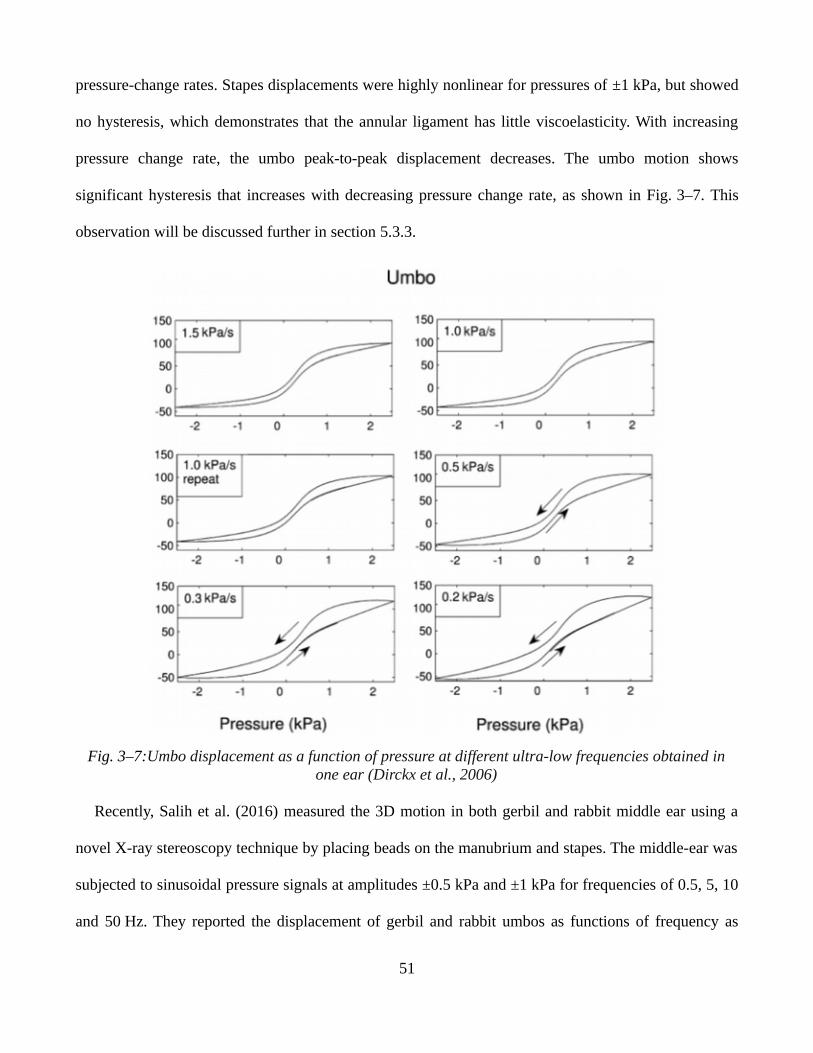
pressure-change rates. Stapes displacements were highly nonlinear for pressures of ±1 kPa, but showed

no hysteresis, which demonstrates that the annular ligament has little viscoelasticity. With increasing

pressure change rate, the umbo peak-to-peak displacement decreases. The umbo motion shows

significant hysteresis that increases with decreasing pressure change rate, as shown in Fig. 3–7. This

observation will be discussed further in section 5.3.3.

Recently, Salih et al. (2016) measured the 3D motion in both gerbil and rabbit middle ear using a

novel X-ray stereoscopy technique by placing beads on the manubrium and stapes. The middle-ear was

subjected to sinusoidal pressure signals at amplitudes ±0.5 kPa and ±1 kPa for frequencies of 0.5, 5, 10

and 50 Hz. They reported the displacement of gerbil and rabbit umbos as functions of frequency as

51

Fig. 3–7:Umbo displacement as a function of pressure at different ultra-low frequencies obtained inone ear (Dirckx et al., 2006)

shown in Fig 3–8. Similar to the earlier experiment performed by the same group (i.e., Dirckx et al.,

2006), strong nonlinearity in the stapes motion was obtained, and asymmetry in both umbo and stapes

displacement was obtained with higher displacements for positive pressures. Unlike the case in the

earlier experiment, both umbo and stapes peak-to-peak displacements increased as a function of

frequency. The umbo and stapes were reported to move in opposite directions, but no explanation of

this strange behaviour was suggested. Hysteresis was not reported because “the current experimental

setup does not not currently allow the measurement of displacement direction”.

3.4.4 Pressurized TM vibrations

3.4.4.1 Tympanometric measurements

Tympanometry is well established and widely used to assess middle-ear function in clinical and

scientific studies. From early work (e.g., Decraemer et al., 1984; Shanks & Wilson, 1986), it is well

known that the direction of the pressure sweep affects the admittance measures. In bidirectional

tympanometry, two different peak pressures are found corresponding to the negative and positive

directions of pressure change. The difference between the peaks obtained during the increasing and

decreasing part of the pressure cycle is defined as the peak pressure difference. There are discrepancies

between different studies about how the pressure-change rate affects the pressure peak difference and

52

Fig. 3–8: Displacement of (a) gerbil umbos and (b) rabbit umbos at frequencies of 0.5, 5, 10, and50 Hz (Salih et al., 2016)

what is the cause of the separation between the peaks. Osguthorpe and Lam (1981) studied the effects

of the rate and direction of pressure change on tympanometry in cats. They measured both the

susceptance and conductance components of admittance. Ascending and descending pressure runs

between +3.9 and −5.9 kPa were compared, with rates of pressure change of 100 and 500 Pa/sec. They

observed that the tympanograms for descending runs were simple and single peak, while the ascending

runs produced notched tympanograms. Lower admittance values were obtained with decreasing rates of

pressure change for both ascending and descending runs. Osguthorpe & Lam also investigated the

stability of tympanograms in response to repetitive testing, in both cats and human subjects. The

resulting susceptance and conductance tympanograms of the first, third and tenth descending runs in a

typical human subject were different and did not seem to reach a steady state. Gaihede (1996)

investigated the effects of the rate of pressure change on the increased compliance that occurs as a

result of repetitive loading-unloading experiments (e.g., Osguthorpe & Lam, 1981). He performed 9

tympanometric measurements in healthy adults with different rates of ear-canal pressure change: 500,

1000, 2000 and 4000 Pa/s. For each group he observed that compliance increases in each trial until it

reaches a steady preconditioned state for later trials. He also observed that tympanometric admittance

increased with increasing rates of pressure change. In a more recent article using a modern high-speed

tympanometer (Therkildsen & Gaihede, 2005), no significant effect of pressure change rate was found

on the peak pressure differences for pressure change rates ranging from 500 Pa/s to 4000 Pa/s. A

constant peak pressure difference of 120 Pa was found for all pressure change rates. Therkildsen and

Gaihede (2005) attributed it to hysteresis in the ear and attributed earlier observations of rate

dependence to phase delay in the older instruments.

3.4.4.2 Laser Doppler vibrometry measurements

Lee and Rosowski (2001) used LDV to analyze the acoustic behaviour of the PT and PF of the gerbil in

53

response to middle-ear static pressure sweeps that mimic pressure changes in normal tympanometry.

They measured sound-induced umbo velocity in live gerbils at different levels of static pressure in the

±3 kPa range. Negative middle-ear pressures reduced the velocity magnitude of the TM more than

positive pressures did. This asymmetry between negative pressures and positive pressures is consistent

with other studies (e.g., Dirckx & Decraemer, 2001; Dirckx et al., 2006; Salih et al., 2016). They

reported a dependence of the velocity measurements on the direction of the pressure sweep and

attributed it to hysteresis. They also highlighted the frequency dependence of both the umbo and PF

transfer functions. Umbo velocity increased with the frequency of the sound stimulus from 250 Hz up

to 2.5 kHz and then decreased at higher frequencies for both positive and negative quasi-static

pressures. However, the magnitude of the effect varied with the sign of the static pressure, decreasing

more for negative pressures than for positive pressures for frequencies less than 2.5 kHz.

Gan et al. (2006) used two laser vibrometers to simultaneously measure the umbo and stapes

vibrations in human temporal bones with intact and removed cochlea and a step-wise variation of

middle-ear pressures. They reported displacement responses of the umbo from seven temporal bones,

recorded over the frequency range from 0.2 to 8 kHz in response to positive and negative middle-ear

pressures in the range ±2 kPa and with an acoustic stimulus of 90 dB. They found that positive and

negative pressures in the middle-ear reduced the displacement of the umbo and footplate at frequencies

less than 1500 Hz, while no effect was observed at higher frequencies. This reduction in umbo

displacement for frequencies lower than 1500 Hz is consistent with data reported by Lee and Rosowski

(2001) except that the latter study found that the umbo velocity decreases at frequencies less than

2500 Hz. No asymmetry was detected in the umbo displacement for the intact cochlea, unlike the

results of Lee and Rosowski (2001). These differences between the two studies may be due to the

difference in species as well as to different techniques for measuring vibrations.

In our group, Shapiro (2014) performed preliminary post mortem LDV multiple-point measurements

54

on the pressurized gerbil middle-ear in response to a chirp over the range of 0.2 to 11 kHz. Quasi-static

pressure was varied in both positive and negative directions in a stepwise fashion with measurements

taken at 0, ±0.25, ±0.5, ±1, ±2 and ±2.5 kPa, with each step maintained for 20 s. The vibration

responses of the TM to pressurization were reported for different locations on the PT, PF and

manubrium. Pressurized responses exhibited magnitude reductions at lower frequencies, then rose to a

peak and exhibited sharp features at higher frequencies. As pressure increased, magnitudes decreased

and the peak was shifted to higher frequencies. With regard to hysteresis and cycle-to-cycle changes,

these preliminary results were not repeatable. Kose et al. (2017) extended this work and presented

preliminary results from similar experiments on in vivo gerbils. Vibration responses were similar to

those of Shapiro.

Investigating the presence of hysteresis and the effects of pressure-change rate is ongoing work to

provide a better understanding of the effect of static pressurization on the response of the middle ear.

55

Chapter 4: Methods

4.1 IntroductionDetails regarding the FE modelling are presented in this chapter. It includes a description of the

geometry, model components and mesh in section 4.2. The boundary conditions are defined in

section 4.3. Material properties of the components of the model are presented in section 4.4. Loading

conditions and the time-step analysis are summarized in section 4.5, and the mesh-convergence

analysis is presented in section 4.6.

4.2 Geometry, model components and meshThe 3D geometry of the model is a simplification of the one used by Maftoon et al. (2015), which was

a refinement of the ones used by Elkhouri et al. (2006) and Decraemer et al. (2011). The model of

Maftoon et al. has a fine mesh composed of about 50000 second-order solid elements. Using this mesh

in a dynamic nonlinear viscoelastic analysis is computationally very expensive. Quasi-static pressure

sweeps in clinical tympanometry over a couple of cycles may last a few seconds. For research

tympanometry, an exploration of conditioning effects at low pump speeds results in a set of several

cycles that may last a few minutes. The acoustic stimulus applied as pure tones or chirps may have

frequencies as high as 8 kHz. The time step in simulations of tympanometry should be on the order of

10−5 s to adequately model the response to the acoustic stimulus of frequency 8 kHz (see section 4.5).

Considering this small time step and the long duration of quasi-static pressure sweeps, millions of time

steps are required for these simulations. Thus, for a preliminary study of the response of the middle ear

to conditions similar to tympanometry, we decided to simplify the model and include only the parts that

we expect to contribute the most to the middle-ear response.

The geometry of the model of Maftoon et al. was based on segmentation of a microCT dataset,

supplemented by histological images. The model here includes the PT and PF, the manubrium, and a

56

crude representation of the ossicular chain with a fixed axis of rotation and the cochlear load. The FE

model used in this study is shown in Fig. 4–1. In-house FE preprocessing software, Fie, Tr3 and Fad,

was used by Elkhouri et al. and Maftoon et al. to perform image segmentation and surface tesselation

and to prepare surface meshes for volume mesh generation using the open-source software Gmsh

(Geuzaine & Remacle, 2009). Fad was then used to export the 3D mesh to text files that can be read by

two open-source software packages, Salome-Meca (2016) and Preview (version 1.20.4), the

preprocessors for the FE solvers Code_Aster (version 12.7) and FEBio (version 2.6.4), respectively.

We decided to use these two FE solvers because they are open-source and free/libre software; they

are powerful and well supported; and our group has previously used them in several studies

(Code_Aster: e.g., Maftoon et al., 2015, and Motallebzadeh et al., 2017; FEBio: e.g., Motallebzadeh et

al., 2013, and Soleimani & Funnell, 2016). Our previous simulations using Code_Aster were either

static or dynamic, while all our previous FEBio studies were static. Furthermore, the only viscoelastic

nonlinear model study in our group was performed using FEBio and was static ( Motallebzadeh et al.,

2013). Thus, despite our experience with these solvers, we have not tested the performance of either

one for the new combination of dynamics, nonlinearity and viscoelasticity required for this study. We

therefore decided to create the model for both solvers, and to compare the responses for model

verification.

57

Fig. 4–1:3D FE model of gerbil middle ear. A: components of the model. B: Mesh of the model isshown.

As discussed in section 3.3.2.4, the TM is a complex structure composed of multiple layers. It is an

inhomogeneous structure with anisotropy in the radial, circumferential and through-thickness

directions. However, in this study we assume the TM to be homogeneous and isotropic. This has been

done in many other middle-ear modelling studies, including Maftoon et al. (2015), and has been quite

successful.

In the model of Maftoon et al. (2015), the TM was modelled using Code_Aster’s seven-node

second-order TRIA7 COQUE_3D shell elements. The PT had a variable thickness calculated using an

interpolation algorithm developed to reconstruct a thickness map based on the measurements of

Kuypers er al. (2005), who reported thicknesses along four lines across the PT and eight lines across

the PF in the gerbil, as shown in Fig. 4–2. For simplicity, in our model we used a constant thickness of

15.78 μm (calculated by us to be the mean) for the PT and 23.5 μm (their reported mean) for the PF.

These mean values for the thicknesses of the PT and PF are similar to the measurements of Teoh et al.

(1997) who obtained a mean value of 19.1 μm (SD=3.2) for the PT and a mean of 32.2 μm (SD=12.7)

for the PF based on a histological study on five gerbils.

58

Fig. 4–2: Contour plots of the thickness distribution of a gerbil TM. A: PT; B: PF (Source: Kuypers etal., 2005)

In the model of Maftoon et al. (2015), in order to ensure correct coupling between the shell elements of

the TM and the 3D solid elements of the malleus, the PT was continued over the lateral surface of the

manubrium and nodes were shared between the two structures. This surface was thus modelled with

second-order TRIA7 COQUE_3D shell elements and assigned a thickness of 40 μm. COQUE_3D shell

elements in Code_Aster support nonlinear geometry (large displacements and large rotations) but they

do not support material nonlinearity. Furthermore, testing shell elements in FEBio with simple

geometries (e.g., clamped square plates) for which we have analytical solutions showed no

convergence to the analytical solution in static analysis and showed abnormal behaviour in dynamic

analysis. On the other hand, solid elements in both FEBio and Code_Aster concur well with analytical

solutions, show normal dynamic behaviour with simple geometries, and support material nonlinearity.

We therefore modelled the manubrium with solid elements. We assigned it a larger thickness of 80 μm

that ensured its rigidity under both quasi-static and acoustic pressures, consistent with the model of

Maftoon et al. (2015) and their experimental observations at frequencies below 1600 Hz (e.g., Maftoon

et al., 2013, 2014). In Code_Aster, we use the CREA_MAILLAGE module with its subfunction

COQU_VOLU to build volume meshes for the TM and manubrium from the data of the surface mesh

by extrusion along the normals of the elements. The PT was extruded in one layer, the PF in two layers

and the manubrium in three layers. This operation applies only to first-order meshes, so the second-

order shell elements of the TM and the manubrium were converted to first-order elements before the

extrusion. The resulting solid mesh for the TM and the manubrium was made of first-order PENTA6

3D pentahedral elements. Each node of this type of element possesses three translational degrees of

freedom and no rotational degrees of freedom. Higher-order solid elements are less stiff than first-order

solid elements, give better displacement predictions and have better convergence rates (e.g., Cifuentes

& Kalbag, 1992). The first-order pentahedral elements in Code_Aster can be converted to higher-order

pentahedral elements PENTA15 and PENTA18. On the other hand, FEBio has higher-order hexahedral

59

and tetrahedral elements but supports only first-order pentahedral elements. To have a working model

in both FEBio and Code_Aster, the Code_Aster solid model was converted into a triangulated surface

in Salome_Meca. Then, MATLAB code was written to convert the 3D surface information

corresponding to the solid model of the TM and manubrium to a file type readable by Fad, which in

turn produced a file readable by Gmsh. Using Gmsh, we converted the surface meshes to volume

meshes made of tetrahedral elements. Consequently, a model of the TM and manubrium made of ten-

node second-order tetrahedral solid elements is available for both FEBio (tet10) and Code_Aster

(TETRA10).

The effect of the number of layers in the PT, PF and manubrium was tested. To ensure the continuity

of the layers across the boundaries of these three components, when the PT (which has the smallest

thickness) was extruded to a certain thickness, all other components were extruded by the same amount

as well. Then, when we extruded PF (which has a thickness higher than the PT but lower than the

manubrium) to its required thickness, the manubrium was also extruded by the same amount. Finally,

the manubrium (which has the greatest thickness) was extruded to its required thickness. We evaluated

different configurations for the number of layers, with a maximum of 4 layers for the PT, 5 layers for

the PF and 6 layers for the manubrium. We found that with second-order elements all of the

configurations produced very similar results.

The effective load exerted on the eardrum by the ossicular chain has been modelled by considering a

fixed axis of rotation. Its position was defined by two points corresponding to the most anterior point

on the anterior mallear process and the most posterior point on the posterior incudal process. Stiff

tetrahedral elements, forming what we call the “wedge”, connect the axis of rotation to the upper end of

the manubrium. An additional block of tetrahedral elements is added on top of the wedge to represent

the stiffening effects of the ossicles and middle-ear ligaments. Funnell and Laszlo (1975, 1978)

attempted to estimate the mechanical properties of the ossicles and middle-ear ligaments of the cat

60

based on their geometries. An alternative approach to that a priori parameter estimation is to estimate

the cochlear and ossicular load by fitting to either experimental or model results. Here, the mechanical

properties of the wedge and block were estimated by fitting to the umbo displacements obtained from

the model of Maftoon et al. (2015). A more detailed description will be provided in sections 4.4.2 and

4.4.3. The assumption of rigid-body motion about a fixed axis of rotation is valid up to about 1600 Hz

according to the experimental observations by Maftoon et al. (2013, 2014). For higher frequencies, they

found that the position of the axis of rotation shifts and the manubrium seems to be bending, which is

also consistent with measurements by de La Rochefoucauld and Olson (2010) and Decraemer et al.

(2011). Thus, the findings of our model at higher frequencies may not properly reflect the mechanisms

involved in the gerbil middle ear.

4.3 Boundary conditions Three constraint representations have been implemented in the literature in order describe the

boundaries of the PT and PF: (1) a fully clamped (i.e, all of the three translational and three rotational

degrees of freedom are set to zero) or simply supported (i.e, the three translational degrees of freedom

are set to zero but the rotational degrees of freedom are not) periphery (e.g., Elkhouri et al., 2006;

Maftoon et al., 2014); (2) representation of the tympanic annulus as a shell or a solid structure (e.g.,

Van Wijhe et al., 2000); or a spring restraint at the periphery of the TM (e.g., Koike et al., 2002; Kelly

et al., 2003). The choice of considering the whole TM to be firmly anchored to the bony tympanic

annulus around its entire circumference represents an approximation of the TM anatomy. In fact, the

TM thickens around the periphery of the PT, forming the fibrocartilaginous ring. This structure is

firmly attached to a sulcus in the bony tympanic annulus except superiorly between the PT and PF

(e.g., Gea et al., 2010; Aernouts & Dirckx, 2011). Gea et al. (2010) demonstrated that the boundaries of

the PT and PF are neither simply supported nor fully clamped, suggesting that the fibrocartilaginous

61

ring should be modelled. However, for simplicity, in this model, the PT and PF were considered to be

fully clamped around their peripheries except at their interface. For the superior edge of the wedge, all

three translational degrees of freedom were also set to zero to define a fixed axis of rotation (Fig. 4–3).

The upper face of the block was also clamped.

4.4 Material PropertiesBecause of the scarcity of data in the literature about the material properties of the gerbil middle ear, all

of the parameters describing the material properties of the components were estimated. To define the

baseline parameters, we evaluated the dynamic response of the model to a unit-step sound pressure,

computed frequency responses, and compared them with those from the linear FE model of the gerbil

middle ear of Maftoon et al. (2015). That model generated frequency responses that were similar to

responses measured in vivo using multi-point vibrometry by the same authors (2013, 2014) and to those

measured by other groups (e.g., Lee & Rosowski, 2001) as shown in section 5.2.2.

4.4.1 Tympanic membrane

4.4.1.1 Governing equations

Different approaches have been used in the literature to derive the constitutive equations for nonlinear

viscoelastic materials. In this study, we use a model similar to that of Motallabzadeh (2013) and assume

linear viscosity and nonlinear elasticity (hyperelasticity). The stress response of the material is

62

Fig. 4–3: Illustration of the boundary conditions at the wedge and block.

formulated in terms of a convolution of a time-dependent component and an elastic component, similar

to what is done for small-strain viscoelasticity (linear viscoelasticity). We refer here to this model as a

quasi-linear visco-hyperelastic (QLVH) model. The total second Piola-Kirchhof stress tensor S(t) is

calculated by convolving a normalized relaxation function G(t) with the derivative of an elastic

response function Se:

S (t )=∫0

t

G( t−u)(d S e

d u)d u (4–1)

where t is time and u is a dummy variable. A Prony (exponential) series representation is used for G(t).

This formulation can interconvert the viscoelastic functions between the time and frequency domains,

and also allows a simple discretization procedure for numerical implementation (e.g., Park & Schapery,

1999). Depending on whether Se represents the instantaneous or long-term elastic response, G(t) is

given by either

G(t)=1−∑i=1

N

gi(1−exp(−t / τi)) (4–2)

or

G(t)=1+∑i=1

N

g iexp (−t / τ i) (4–3)

respectively. In both equations, gi (relaxation coefficients) and τi (time constants) are material

parameters and N is the number of exponential terms.

Among the many constitutive models that have been proposed for hyperelastic materials, the

Mooney-Rivlin method has been widely used to simulate deformations in nearly incompressible soft

tissues (e.g., Martins et al., 2006) such as the TM (e.g., Wang et al., 2007). According to this model, a

strain energy W composed of deviatoric and volumetric energies (i.e., energies due to distortion and to

change of volume, respectively) is defined by

W=C10( I 1−3)+C01( I 2−3)+W vol (J ) (4–4)

63

where I1 and I2 are the invariants of the deviatoric part of the right Cauchy-Green deformation tensor

and are related to the strain invariants as follows:

I1=J−2

3 I1

I2=J−4

3 I2

. (4–5)

C10 and C01 are material coefficients; and Wvol(J) is the volumetric part of the energy function with this

form in our model:

W vol=K ( ln J )2 (4–6)

where J = λ1λ2λ3 is the determinant of the elastic deformation gradient; the λi are the stretches; and K is

the bulk modulus. Soft tissue is generally assumed to be nearly incompressible (e.g., Humphrey, 2003).

Thus, volume change is negligible, and the bulk modulus is set high enough to make Wvol very small.

Material parameters for a hyperelastic material can be determined by performing an unconfined

tensile or compression test (to determine the deviatoric properties) and a confined compression test (to

determine the volumetric part of the strain energy function). Under small strains, the Young’s modulus

of the material may be written as follows:

E=4 (C10+C 01)(1+ν) , (4–7)

where ν is Poisson’s ratio and the bulk modulus is defined as

K=4 (C10+C01)(1+ν)

3 (1−2 ν). (4–8)

In the Mooney-Rivlin model, the bulk modulus can be given by (Delalleau et al., 2008)

K=4 (C10+C01)

3(1−2ν)(4–9)

In the case of quasi-incompressibility, the effect of the bulk modulus is insignificant.

This QLVH model is readily available in FEBio but is not implemented in Code_Aster. It is possible

to add it, however, using MFront (http://tfel.sourceforge.net/), a constitutive law generator which

comes in the form of a software library that provides interfaces to several mechanical solvers, including

64

Code_Aster. MFront (version 2.3) makes it possible to define a constitutive law without having to

worry about the solution methods. It converts domain-specific languages into C++ and offers three

kinds of material knowledge: (1) material properties (e.g., the Young’s modulus, Poisson’s ratio, bulk

modulus, etc.); (2) mechanical behaviours (e.g., Ogden model, Chaboche model, etc.); and (3) simple

point-wise models (e.g., material swelling used in fuel performance codes). The coupling between

Code_Aster and MFront has been extensively tested and its effectiveness demonstrated for many laws.

The implementation of different mechanical behaviours is compatible with solid, shell, plate and joint

elements. MFront is adapted to both implicit and explicit temporal schemes. For finite strains, it

suffices to define the stress tensor and the consistent tangent operator. The latter is a term introduced by

Simo and Taylor (1986) and plays an important role in the nonlinear FE method. It is defined as the

ratio of the stress tensor to the strain tensor and is a fourth-order tensor:

D=∂ S∂ E

=2∂S∂C

(4–10)

where S is the second Piola-Kirchhoff stress; and C is the right Cauchy-Green tensor.

For the numerical solution of QLVH problems with the use of the Newton-Raphson method, it is

necessary to determine the consistent tangent operator at each integration point. This allows one to

obtain a quadratic rate of asymptotic convergence when using the Newton-Raphson method (Simo &

Hughes, 2006). For relatively simple models, such as a Mooney-Rivlin model, it is possible to

determine it analytically. However, in the case of more complex models such as a QLVH model, it is

necessary to use an approximation.

The numerical approximation consists of transforming the convolution representation presented in

equation 4–1 and discussed in section 3.3.2.3 into a two-step recurrence formula involving internal

variables stored at the quadrature points of elements. This method was first suggested by Hermann and

Petterson (1968) and Taylor et al. (1970). This approximation is only valid for a particular class of

65

relaxation functions consisting of a linear combination in time like the one we are using (i.e., Prony

series, equation 4–3). For a detailed overview of the recursive procedure for updating the Cauchy stress

tensor and consistent tangent operator, refer to the work of Simo and Hughes (2006, p. 372).

Code_Aster provides two different finite-strain formulations (1) SIMO_MIEHE and

(2) GROT_GDEP, where the principal of virtual work is expressed in the current configuration and in

the reference configuration, respectively, and the Cauchy stress and second Piola-Kirchhoff stress are

the respective outputs. The GROT_GDEP formulation is also called “total Lagrangian” in the literature

(Belytschko et al., 2013). When using MFront, finite-strain behaviours must use the SIMO_MIEHE

finite-strain formulation. Thus, in MFront, both the stress and the consistent tangent operator must be

provided in the current configuration. MFront has intrinsic functions to transform tensors from one

configuration to another, such as convertSecondPiolaKirchhoffStressToCauchyStress for stress-tensor

transformation and pull_back for transformation of the consistent tangent operator to the current

configuration.

4.4.1.2 Viscoelastic parameters

The acoustic stimulus in wideband tympanometry and LDV experiments is usually within the range

150 to 8000 Hz. The linear change rate of the quasi-static pressure in tympanometry and in sweep

pressurization experiments on the middle-ear vary from 50 Pa/s to 4000 Pa/s. A 50 Pa/s

pressure-change rate in a triangular pressure signal between +2.5 kPa and −2.5 kPa corresponds to a

frequency of 5 mHz (200 sbeing the time it takes for the signal to pass from −2.5 kPa to +2.5 kPa and

back again in a triangular pressure signal . The period of the signal is thus 200 s and the frequency is

1/200 s=5 mHz) while a rate of 4000 Pa/s for the same pressure range corresponds to a frequency of

400 mHz. In this study, we only examine the response of the middle ear to pressure change rates from

±200 Pa/s (20 mHz) to ±1500 Pa/s (150 mHz).

66

To cover the range from the ultra-low frequencies of the quasi-static pressure variations to the high

frequencies of the acoustic stimulus, for both the PT and the PF we predefine six time constants that

cover the range of 3 mHz to 16 kHz. A common practice is to take one time constant per decade in the

time domain (e.g., Knauss & Zhao, 2007). This also corresponds to one time constant per decade in the

frequency domain (e.g., Fung, 2013; Charlebois et al., 2013). The inverse of each time constant

corresponds to an angular frequency (ωi=1/τi=2πfi) for which the damping represented by the

coefficient (gi) is maximum. Since we limit the number of time constants to six (due to a restriction in

FEBio), we use time constants ranging from 10 µs(=100000 rad/s ≈16 kHz) to 52 s (=0.019 rad/s

≈3 mHz) that are approximately equally logarithmically spaced to cover the frequency range of

interest. In this case, we end up having about one time constant per two decades: τ1=10 µs, τ2=220 µs,

τ3=5 ms, τ4=0.11 s, τ5=2.3 s and τ6=52 s.

Each term in a Prony series involves the two parameters gi (relaxation coefficient) and τi (time

constant), resulting in two degrees of freedom (DOFs). The relaxation coefficient represents the amount

of damping at the frequency corresponding to the time constant. As discussed in section 3.3.2.3, for an

n-term series, the sum of the n relaxation coefficients needs to be less than or equal to 1 (Simo &

Hughes, 2006, p. 349). A common characteristic of the hysteresis of soft tissues is its insensitivity to

frequency, with a continuous relaxation spectrum over a wide range of frequencies as shown in

Fig. 4–4. This suggests that one should consider equal relaxation coefficients for all of the time

constants. Thus, taking into account the constraint on the sum of the relaxation coefficients (Eq 3–19),

each of the six equal coefficients must be greater than 0 and less than or equal to 1/6 ≈0.167). A We

evaluated the dynamic response of the model to sound pressure using these parameters and compared it

to the results from the linear FE model of the gerbil middle ear of Maftoon et al. (2015). We compared

our model results at the umbo, two points in the PT (anterior and posterior) and a centre point in the PF

to results from the model of Maftoon et al. (2015). We found that the a coefficient 0.07 for all time

67

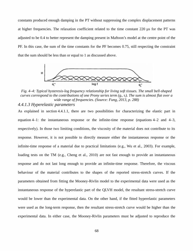
constants produced enough damping in the PT without suppressing the complex displacement patterns

at higher frequencies. The relaxation coefficient related to the time constant 220 µs for the PT was

adjusted to be 0.4 to better represent the damping present in Maftoon’s model at the centre point of the

PF. In this case, the sum of the time constants for the PF becomes 0.75, still respecting the constraint

that the sum should be less than or equal to 1 as discussed above.

4.4.1.3 Hyperelastic parameters

As explained in section 4.4.1.1, there are two possibilities for characterizing the elastic part in

equation 4–1: the instantaneous response or the infinite-time response (equations 4–2 and 4–3,

respectively). In those two limiting conditions, the viscosity of the material does not contribute to its

response. However, it is not possible to directly measure either the instantaneous response or the

infinite-time response of a material due to practical limitations (e.g., Wu et al., 2003). For example,

loading tests on the TM (e.g., Cheng et al., 2010) are not fast enough to provide an instantaneous

response and do not last long enough to provide an infinite-time response. Therefore, the viscous

behaviour of the material contributes to the shapes of the reported stress-stretch curves. If the

parameters obtained from fitting the Mooney-Rivlin model to the experimental data were used as the

instantaneous response of the hyperelastic part of the QLVH model, the resultant stress-stretch curve

would be lower than the experimental data. On the other hand, if the fitted hyperelastic parameters

were used as the long-term response, then the resultant stress-stretch curve would be higher than the

experimental data. In either case, the Mooney-Rivlin parameters must be adjusted to reproduce the

68

Fig. 4–4: Typical hysteresis-log frequency relationship for living soft tissues. The small bell-shapedcurves correspond to the contributions of one Prony series term (gi, τi). The sum is almost flat over a

wide range of frequencies. (Source: Fung, 2013, p. 288)

experimental curves (e.g., Motallebzadeh et al., 2013). We have chosen to take the elastic part of the

model to be the instantaneous elastic response and the Prony series of equation 4–3 is therefore used as

the time-dependent part.

The parameters in Table 4–1 were obtained by matching the responses at the umbo and at the centre

of the PF from the model of Maftoon et al. (2015). For the PT, these Mooney-Rivlin coefficients

correspond to a small-displacement Young’s modulus (obtained from equation 4–7) of 9.9 MPa,

compared with 10 MPa as used by Maftoon et al. (2015). In our model, different ratios of C10 to C01

were studied, namely, 1:0, 1:1,0:1, 1:2, 2:1, 1:3 and 3:1, while keeping the sum of C10 and C01 constant

at 1.6787 MPa. The model responses to both sound pressures and quasi-static pressures were found to

be insensitive to the C10:C01 ratio when the sum of C10 and C01 remains constant. This is consistent with

the results of Qi et al. (2008) who used the Mooney-Rivlin model for the soft tissue in a newborn

middle-ear model and found that the different combinations of C10 and C01 had little effect on model

displacements in response to static pressures of ±3 kPa. Thus, for the PT, we select a C10:C01 ratio equal

to 3:1 as an arbitrary choice.

The density of the PT was initially defined to be 1100 kg/m3 as in the model of Maftoon et al.

(2015), the value having been chosen as being between the density of water (1000 kg/m3) and that of

undehydrated collagen (1200 kg/m3) (Funnell & Laszlo, 1978). It was then changed to be equal to

1300 kg/m3 in order to match the resonance frequency obtained by Maftoon et al. (2015) at the umbo

and at points on the anterior and posterior PT. Alternatively, we could have reduced the effective

Young’s modulus by reducing the sum of the Mooney-Rivlin coefficients. In that case we would have

had to adjust the ossicular load to stiffen the response at the lower frequencies.

For the PF, we defined the density to be 1100 kg/m3 and adjusted the Mooney-Rivlin coefficients to

match the model response of Maftoon et al. (2015) at the centre of the PF. The Mooney-Rivlin

coefficients for the PF were taken to be C10=81.2 kPa and C01=40.6 kPa, which correspond to a small-

69

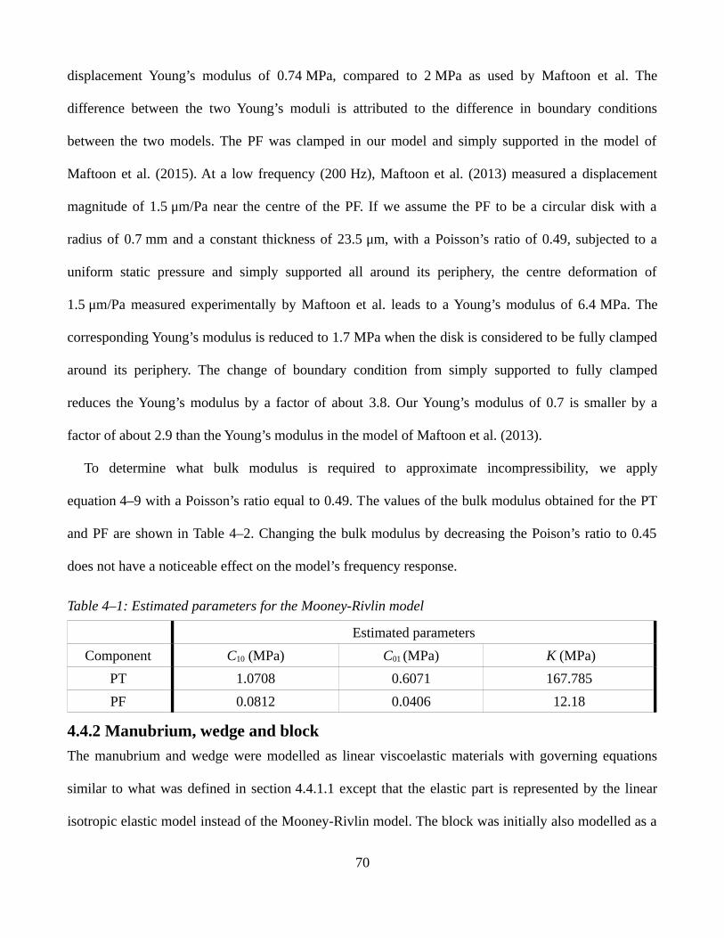
displacement Young’s modulus of 0.74 MPa, compared to 2 MPa as used by Maftoon et al. The

difference between the two Young’s moduli is attributed to the difference in boundary conditions

between the two models. The PF was clamped in our model and simply supported in the model of

Maftoon et al. (2015). At a low frequency (200 Hz), Maftoon et al. (2013) measured a displacement

magnitude of 1.5 μm/Pa near the centre of the PF. If we assume the PF to be a circular disk with a

radius of 0.7 mm and a constant thickness of 23.5 μm, with a Poisson’s ratio of 0.49, subjected to a

uniform static pressure and simply supported all around its periphery, the centre deformation of

1.5 μm/Pa measured experimentally by Maftoon et al. leads to a Young’s modulus of 6.4 MPa. The

corresponding Young’s modulus is reduced to 1.7 MPa when the disk is considered to be fully clamped

around its periphery. The change of boundary condition from simply supported to fully clamped

reduces the Young’s modulus by a factor of about 3.8. Our Young’s modulus of 0.7 is smaller by a

factor of about 2.9 than the Young’s modulus in the model of Maftoon et al. (2013).

To determine what bulk modulus is required to approximate incompressibility, we apply

equation 4–9 with a Poisson’s ratio equal to 0.49. The values of the bulk modulus obtained for the PT

and PF are shown in Table 4–2. Changing the bulk modulus by decreasing the Poison’s ratio to 0.45

does not have a noticeable effect on the model’s frequency response.

Table 4–1: Estimated parameters for the Mooney-Rivlin model

Estimated parameters

Component C10 (MPa) C01 (MPa) K (MPa)

PT 1.0708 0.6071 167.785

PF 0.0812 0.0406 12.18

4.4.2 Manubrium, wedge and block

The manubrium and wedge were modelled as linear viscoelastic materials with governing equations

similar to what was defined in section 4.4.1.1 except that the elastic part is represented by the linear

isotropic elastic model instead of the Mooney-Rivlin model. The block was initially also modelled as a

70

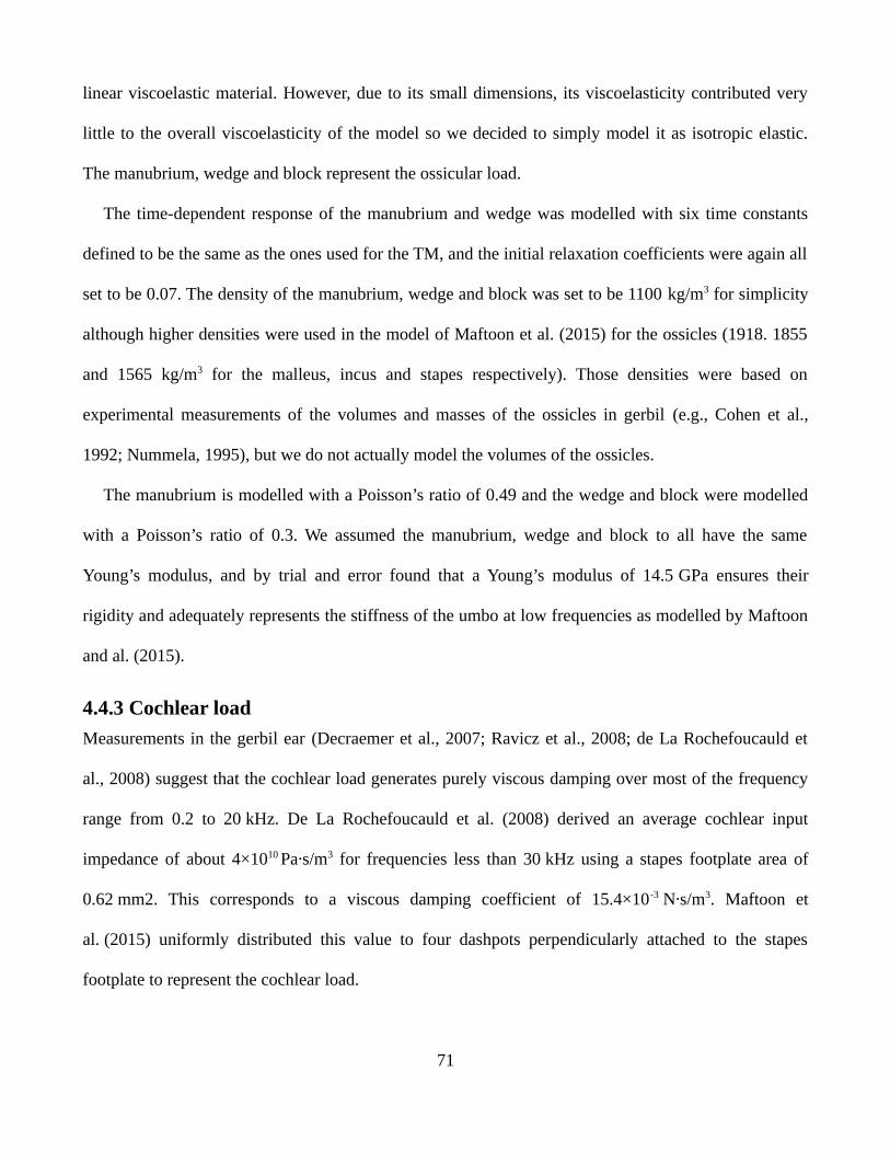
linear viscoelastic material. However, due to its small dimensions, its viscoelasticity contributed very

little to the overall viscoelasticity of the model so we decided to simply model it as isotropic elastic.

The manubrium, wedge and block represent the ossicular load.

The time-dependent response of the manubrium and wedge was modelled with six time constants

defined to be the same as the ones used for the TM, and the initial relaxation coefficients were again all

set to be 0.07. The density of the manubrium, wedge and block was set to be 1100 kg/m3 for simplicity

although higher densities were used in the model of Maftoon et al. (2015) for the ossicles (1918. 1855

and 1565 kg/m3 for the malleus, incus and stapes respectively). Those densities were based on

experimental measurements of the volumes and masses of the ossicles in gerbil (e.g., Cohen et al.,

1992; Nummela, 1995), but we do not actually model the volumes of the ossicles.

The manubrium is modelled with a Poisson’s ratio of 0.49 and the wedge and block were modelled

with a Poisson’s ratio of 0.3. We assumed the manubrium, wedge and block to all have the same

Young’s modulus, and by trial and error found that a Young’s modulus of 14.5 GPa ensures their

rigidity and adequately represents the stiffness of the umbo at low frequencies as modelled by Maftoon

and al. (2015).

4.4.3 Cochlear load

Measurements in the gerbil ear (Decraemer et al., 2007; Ravicz et al., 2008; de La Rochefoucauld et

al., 2008) suggest that the cochlear load generates purely viscous damping over most of the frequency

range from 0.2 to 20 kHz. De La Rochefoucauld et al. (2008) derived an average cochlear input

impedance of about 4×1010 Pa·s/m3 for frequencies less than 30 kHz using a stapes footplate area of

0.62 mm2. This corresponds to a viscous damping coefficient of 15.4×10-3 N·s/m3. Maftoon et

al. (2015) uniformly distributed this value to four dashpots perpendicularly attached to the stapes

footplate to represent the cochlear load.

71

In Maftoon's model, cochlear damping was modelling by placing four dashpots perpendicular to the

stapes footplate. The total viscous damping coefficients was equal to 15.4×10-3 N·s/m3. Following the

same approach, in our model in Code_Aster, the cochlear load was modelled by a dashpot

perpendicularly attached to the inferior part of the manubrium near the umbo, with a viscous damping

coefficient of 2.04×10-3 N-s/m3. This is smaller than the value of 15.4×10-3 N·s/m3 used in Maftoon’s

model because the damper is attached to the manubrium instead of to the stapes footplate, resulting in a

stronger effect on the TM vibration patterns. This is smaller than the value of 15.4×10-3 N·s/m3 used in

Maftoon’s model because the damper is attached to the manubrium instead of to the stapes footplate,

resulting in a stronger effect on the TM vibration patterns. In our model in FEBio, the cochlear

damping was represented in both the manubrium and wedge by a very high relaxation coefficient equal

to 16 for the time constant 10 µs. This violates the two constraints on the Prony-series coefficients

discussed in section 3.2.3.3, but it can thought of as following the common practice of representing the

cochlea by a first-order mass-spring-dashpot system, where the damping coefficient is set to be higher

than 1 for an overdamped system. Implementing this approach in Code_Aster let to numerical

convergence problems. On the other hand, using discrete dampers in FEBio was not possible because

their dampers are restricted to connecting two rigid bodies. Although the manubrium is assumed to be

rigid, the other end of the damper is a node that does not belong to a rigid body. Introducing an

artificial rigid body to allow the implementation of the damper led to abnormal behaviours. In any case,

even though the two models use different representations of cochlear damping they produce similar

results, as will be shown in section 5.2.

4.5 Loading conditions and time-step analysis We evaluated the response of our gerbil middle-ear model to different loading conditions. As

mentioned in section 4.4, to evaluate the material properties, we applied a unit-step sound pressure of

72

1 Pa on the TM surface and performed transient FE analyses. Simulations were continued for 25 ms

after the onset of the unit-step sound-pressure function. By 25 ms, the velocity magnitudes at different

locations of the TM and manubrium had reached almost zero. Frequency responses were obtained by

differentiating the displacement responses and then computing the fast Fourier transforms of the

resulting velocity responses. The response of our model was compared to the model of Maftoon et al.

(2015). A doubling of the time span of the simulation (from 25 to 50 ms) changed the responses by less

than 0.03 dB, so the time span of 25 ms was used in order to reduce computation time. The selected

time span provided a frequency resolution of 12 Hz.

For the acoustic stimulus, the choice of the time step is crucial and is controlled by its highest

frequency content. Fig. 4–5 shows the effect of the size of the time step on the umbo frequency

response, with time steps of 75, 50, 30, 15, 10 and 5 μs. For time steps between 5 and 30 μs, an

increase of less than 15 nm/Pa in magnitude was observed as the time step increased. Above 4 kHz,

compared with the results for the smallest time step (5 μs), the two largest time steps displayed

discrepancies of up to 3.5 dB followed by dramatic roll-offs above 4 and 8 kHz, respectively. As a

trade-off between accuracy and length of computation time, we chose a time step of 10 μs for our

simulations for this loading condition.

73

We also studied the response of the middle ear to quasi-static triangular pressure stimuli at linear rates

between 200 Pa/s and 1.5 kPa/s with an amplitude of ±2.5 kPa as done in a study by Dirckx et al.

(2006). To obtain stable results, we simulated at least 3 cycles of each pressure-change rate.

Furthermore, in some runs at a pressure-change rate 1.5 kPa/s, a small sinusoidal acoustic stimulus of

1 Pa amplitude was added to the quasi-static pressure for about 0.3 s near the 0 Pa pressure value on

both the ascending (from −2.5 kPa to +2.5 kPa) and descending (from +2.5 kPa to −2.5 kPa) branches

(see Fig. 4–6) to study how the peak pressure (i.e., the static pressure at which the vibration amplitude

is maximal, analogous to the tympanometric peak pressure discussed in section 3.2.1) changes between

the two branches as a function of the pressure-change rate.

74

Fig. 4–5: Effect of size of time step on simulated umbo frequency response.

Fig. 4–6: Illustration of the loading condition for quasi-static pressure-change rate at 1.5 kPa/s with asuperimposed pure tone of 226 Hz. A: Pressure as a function of time with magnification of the acoustic

stimulus (a factor of 100 was applied on the acoustic stimulus for better visualization). B: A closerview of the left-hand rectangle in A. C: A closer view of the right-hand rectangle in A.

For this loading condition without the acoustic stimulus, the largest acceptable time step was equal to

0.05 s and a smaller time step equal to 0.1 ms wasneeded for the faster pump speeds and for modelling

buckling. Thus, the time step was set to vary between 0.05 s and 0.1 ms. When an acoustic stimulus is

applied in addition to the quasi-static pressure, a constant time step of 10 μs was used.

We also studied the response of the middle ear to a quasi-static sinusoidal pressure signal at

75

frequencies of 0.5, 5, 10 and 50 Hz as done in a study by Salih et al. (2016). We simulated at least

about 5 cycles of each frequency. We used the times steps 1 ms and 100, 50 and 10 μs for the

frequencies 0.5, 5, 10 and 50 Hz, respectively, to provide adequate representations of the sinusoids.

We also evaluated the response of our model to a sudden increase in static pressure followed by an

acoustical signal. The pressure was increased linearly from zero to 250 Pa in 1 ms and then maintained.

After 25 ms an acoustical pressure of 94 dB (2 Pa peak to peak) was applied as either a sinusoidal wave

at 226 Hz or a 50 ms chirp with frequency changing linearly from 0.12 to 3 kHz (see Fig. 5–21 and

Fig. 5–22). This loading condition was considered mainly to evaluate the capabilities of the model to

simulate conditions present in step-wise pressurization cycles in LDV experiments (e.g., Shapiro, 2014;

Kose et al., 2017). For these loading condition, a constant time step equal to 10 μs was used to simulate

the vibrations due to pure tone and chirp.

Since the main purpose of this study was to evaluate the response of the gerbil middle ear at specific

locations and to validate the model results against the multi-point experimental data of previous

studies, we chose to extract the displacement values for only a limited set of nodes instead of for all of

the ~28,000 nodes in the model. We considered only two nodes on the manubrium (d and e in

Fig. 4–7), a node on the posterior PT (g), a node on the anterior PT (k) and a node at the centre of the

PF (a).

76

Fig. 4–7: A schematic of the general layout of eighteen micro-beads on a right gerbil TM; the shadedarea represents the remaining hidden region of the PT. (Source: He, 2012)

4.6 Mesh convergence

The original mesh for the TM and manubrium that resulted from conversion of shell elements into a

volume mesh contained about 14600 tetrahedral elements and about 28000 nodes. The model of

Maftoon et al. (2015) had around 80000 nodes. Simplification of the model provides a significant

reduction in the computational cost. To test whether the mesh was fine enough, we used Code_Aster’s

Homard utility (Nicolas & Fouquet, 2013) to refine the mesh by dividing each tetrahedral element into

eight smaller tetrahedral elements. Two iterations of refinement were performed to define two refined

meshes. The first refined mesh resulted in only a 1.4 % increase in the umbo displacement magnitude

in response to sound pressure at the lowest frequency (200 Hz). The second mesh resulted in a further

0.35 % increase in the umbo displacement magnitude. For frequencies between 20 and 2000 Hz, the

first refined mesh resulted in an increase of less than 3% in the umbo displacement magnitude, and for

higher frequencies the difference remained less than 5.3 %. The second refined mesh resulted in a

further 1.8 % increase in the umbo displacement magnitude for frequencies between 200 and 2000 Hz

and an increase of less than 3.2 %for higher frequencies. Based on these results, we chose to perform

this study with the original mesh. The wedge and block meshes were made very coarse (52 tetrahedral

elements in total) because their shapes are not intended to be realistic.

Simulations were done on the supercomputer Guillimin of McGill University. Guillimin is a cluster

of Intel Westmere EP Xeon X5650 and Intel Sandy Bridge EP E5-2670 processors running under the

CentOS 6 Linux distribution. Code_Aster studies were performed using one processor and 4 GB of

RAM. Each simulation for one set of parameters and 2500 time steps lasted about 24 hours. Although a

parallel version of Code_Aster was successfully installed and tested on a lab computer, its

implementation in Guillimin faced some difficulties and was not further investigated. Furthermore,

running parallel Code_Aster on a standard computer is very expensive in terms of memory and disk

space. Thus, we were limited to using a single processor with Code_Aster. FEBio uses OpenMP to

77

parallelize the FE calculations. Parallelism improves the performance considerably. After testing with

up to 16 processors, an increase in the number of processors beyond four showed no improvement. In

fact, using a higher number of processors actually decreased performance. A simulation in FEBio for

one set of parameters and 2500 time steps lasts for about 2 hours with 4 processors, as opposed to

8 hours when using one processor.

78

Chapter 5: Results

5.1 IntroductionIn this chapter, we present the responses of our FE model of the gerbil middle ear to the different

loading conditions described in the previous chapter. In section 5.2, we present the response of the

model to low-amplitude sound pressures. We compare results from the two FE solvers and the results

from the model of Maftoon et al. (2015). In section 5.3, we report the response of the model to high

quasi-static pressures in the form of triangular and sinusoidal signals and in different frequency ranges

as well as the combination of high-static pressures with a low-amplitude pure tone. Simulation results

are compared to experimental measurements from previous studies. In section 5.4, we present the

response of the model to a linearly increasing static pressure followed by low-amplitude sound

pressures, including a pure tone and a chirp.

5.2 Unpressurized vibrations In this section we first present a model verification in which we compare the FEBio and Code_Aster

models in response to sound pressure. Then, we present the frequency responses of our FEBio model at

the umbo and at two nodes on the manubrium, two nodes on the PT and one node on the PF (as

discussed in section 4.5) and compare them with responses of the model of Maftoon et al. (2015) and

previous experimental results.

5.2.1 Comparison of FEBio and Code_Aster

As mentioned in section 4.2, two models of the gerbil middle ear were created, for two different FE

solvers, FEBio and Code_Aster, for model verification. This step ensures that FEBio and Code_Aster

provide the same results for the same material properties and loading conditions to evaluate whether

the model implements our assumptions correctly and to check the consistency of our dynamic

quasi-linear viscoelastic model across different solvers.

79

Fig. 5–1 shows model velocity responses in the time domain for the umbo in both FEBio and

Code_Aster in response to a step of sound pressure. The two FE solvers produce very similar responses

in the z direction (i.e., at right angles to the plane of the annulus of the TM) and in total magnitude.

Ignoring the first three cycles where differences are the largest due to transient effects, we see changes

of less than 3% in velocity magnitude between the two solvers. The responses at other nodes of the

model also show very similar results. Fig. 5–2 shows model responses in the frequency domain, and it

can be seen that the two solvers match very well, and a change of less than 0.05 dB in magnitude was

found for all frequencies between 0.2 and 10 kHz. In terms of computational cost, for the same analysis

and using the same resources (a single processor), an FEBio simulation takes about 8 hours while a

Code_Aster simulation requires about 24 hours for 2500 time steps. Since we gained a certain

confidence in the performance of FEBio for dynamic viscoelastic models, and because of the ease of

implementation of computational parallelism in FEBio (with OpenMP, see section 4.6), most of the

subsequent simulations were conducted in FEBio unless stated otherwise. Even though both solvers

produced almost identical results for this set of parameters and loading conditions, a thorough model

verification would require testing with both solvers every time a modification is made to either material

properties or loading conditions. However, due to the high computational costs of nonlinear dynamic

analysis in Code_Aster, this thorough comparison of the two solvers was not performed. This can be

done later, once the code in Code_Aster is modified for parallel computations for better performance.

80

Fig. 5–1: Comparison of umbo velocity in FEBio and Code_Aster. A: Comparison of velocity in zdirection . B: Comparison of magnitude velocity. The red lines almost completely obscure the blue

lines.

81

5.2.2 Umbo and pars-flaccida responses

As mentioned in section 4.4, the material properties of the components of our model were determined

based on matching the umbo response to that of Maftoon’s model. In earlier experimental studies (e.g.,

Lee and Rosowski, 2001; Rosowski and Lee, 2002; Maftoon et al., 2013; Maftoon et al., 2014), it was

observed that the vibrations of the PF affect responses measured at the umbo. In this section we present

these responses together.

5.2.2.1 Low frequencies

Fig. 5–3 shows that the umbo response from the present model is very similar to that from Maftoon’s

model in the low-frequency range (up to about 1 kHz) except around the resonance frequency of the PF

82

Fig. 5–2: Comparison of frequency responses of umbo in FEBio and Code_Aster. The red lines almostcompletely obscure the blue lines.

near 800 Hz. The magnitude and phase of the umbo at the lowest frequency in the model were

382.7 nm/Pa and −5.4°, compared with 381.4 nm/Pa and −4° in Maftoon’s model, resulting in a

difference of 0.34% for magnitude and −1.4° for phase. The phase at low frequency is very close to

zero as observed in experimental results.

Fig. 5–4 shows simulated responses at the centre of the PF from our model compared to those from

Maftoon’s model. The small-amplitude stiffness of the PF was selected to exactly match the

low-frequency response of Maftoon’s model at the centre of the PF. As mentioned in section 4.3, this

step was necessary to account for the difference in boundary conditions for the PF in the two models

(i.e, fully clamped for the solid elements in our model and simply supported for the shell elements in

Maftoon’s model). The selected Young’s modulus and predefined density of the PF resulted in a

83

Fig. 5–3: Comparison of our gerbil model umbo response with Maftoon’s model

resonance frequency similar to the one obtained in the model of Maftoon et al. The width and

magnitude of the centre of the PF resonance were matched to Maftoon’s model by adjusting the Prony

series coefficient at 220 μs as previously described in section 4.4.1.2. At the lowest frequency the

centre of the PF in our model has a magnitude of 2.6 μm/Pa and a phase of −4.4° compared to a

magnitude of 2.4 μm/Pa and a phase of −1.9°. The difference in magnitude is about 8% for magnitude

and 2.5° for phase. Once again, our model produces a slightly more negative phase.

Fig. 5–5 shows a magnified region of the umbo response from 0.2 to 2 kHz, emphasizing the feature

related to the PF. The PF shows a resonance at about 820 Hz in both our model and Maftoon’s model.

Between about 700 and 950 Hz, the umbo response from our model shows a feature that includes a

shallow maximum (at 790 Hz) followed by a shallow minimum (at 865 Hz) in the magnitude, and a

local minimum (at 840 Hz) in the phase. By comparison, in Maftoon’s model the feature is more

pronounced, with a magnitude maximum (at 780 Hz) followed by a minimum (at 880 Hz) and a phase

minimum (at 840 Hz). According to Maftoon et al. (2013), this feature in the umbo response

corresponds to the resonance of a flat PF and they refer to its role in shunting low-frequency sound.

Rosowski et al. (1997) also observed that a flat PF has larger displacements than the umbo, and also

showed that it has larger displacements than the PT in this low frequency range. Although the

magnitude of the simulated response at the centre of the PF at resonance (800 Hz) is 16 μm/Pa in both

our model and Maftoon’s model, its effect on the umbo response is less in our model. The reason for

these differences will be discussed in section 5.2.4.

84

Fig. 5–4:Comparison of our gerbil PF model response with Maftoon’s model response.

85

Fig. 5–5: A magnified view of part of Fig 5–3 to clearly show the effect of the flat PF on the umboresponse, namely, a maximum and minimum and in the displacement magnitude that corresponds to the

resonance frequency of the PF.

5.2.2.2 Mid and high frequencies

The simulated umbo response in Fig. 5–3 shows a rather broad resonance with a peak of 599 nm/Pa at

1.62 kHz, close to what was obtained with Maftoon’s model with a peak of 605 nm/Pa at 1.60 kHz. The

difference in peak magnitude is less than 1%. The width of the resonance and its magnitude are mainly

controlled by the PT Prony series coefficients and time constants as well as the Prony series coefficient

at the highest frequency for the manubrium and wedge (which represents the cochlear damping). The

location of the resonance frequency of the umbo is mainly controlled by the elastic material properties

of the PT and its density, which were selected to match Maftoon’s model.

86

For both models, the umbo response shows a roll-off with substantial irregularities, with magnitude

changes of a few decibels and phase changes of a few tens of degrees. For frequencies above the

resonance frequency, our simulated umbo responses are different in detail from those from Maftoon’s

model. The differences between the two models increase with increasing frequency, with our model

having mainly lower magnitudes. The slope of the roll-off from 2.5 kHz to 5 kHz is about 7 dB/octave

in our model and 5 dB/octave in Maftoon’s model. At higher frequencies the vibrations of the ossicles

become more complex and the axis of rotation of the middle ear no longer corresponds to the

anatomical axis (e.g., Maftoon et al., 2015). Since our model doesn’t include the geometry of the

ossicles, and the location of the axis of rotation is fixed, it is to be expected that the response of our

model to high frequencies is different from that of Maftoon’s model.

For the PF, the slope of the roll-off from 1 kHz to 2 kHz is equal to 8.7 dB/octave in our model

compared with 9.5 dB in Maftoon’s model. While the magnitude of the PF displacement in Maftoon’s

model keeps decreasing after 2 kHz, our PF model response at higher frequencies shows many more

irregularities than Maftoon’s model does. Above 2 kHz, there are regions where the vibration

magnitude of the PF increases suddenly and then decreases, which indicates that the motion of the PF is

not as damped at high frequencies as it should be. Increasing the Prony series coefficient for 10 μs for

the PF (rather than assuming that it is the same as for the PT) could effectively smooth the

displacement of the PF at the higher frequencies.

Fig. 5–6 shows the umbo responses of our model with and without the cochlear damping and

compares them with Maftoon’s model. It is clear that the cochlear damping plays a major role in

flattening the resonance of the umbo. It is also clear that the damping in the TM and the manubrium

modelled by Prony series in our model is less than the mass-proportional Rayleigh damping in

Maftoon’s model. Whether we underestimated the TM damping and overestimated the cochlear

damping, or Maftoon did the opposite, is not very clear, and cannot be easily determined due to an

87

inherent lack of knowledge of both the TM damping and the cochlear impedance in gerbils. However,

our use of a Prony series is a more realistic representation of the damping in soft tissues and represents

damping in separate frequency ranges, as opposed to the Rayleigh damping in Maftoon’s model that

affects all frequencies with a single parameter. We have initially assumed an internal damping of the

TM that is equal across all frequencies but it is not really clear whether this is actually the case.

Fig. 5–6: Comparison of our model umbo response with that of Maftoon’s model with cochleardamping (CD) and with no cochlear damping (No CD).

The results from Fig. 5–3 to Fig. 5–6 were obtained from our FEBio model. The Code_Aster model,

with the cochlear impedance modelled by a single dashpot as described in section 4.4.3, produced

results very similar to those of the FEBio model except for a small magnitude minimum at about

2.8 kHz and some small differences above 7 kHz, as shown in Fig. 5–7.

88

Fig. 5–7: Comparison of the umbo response of FEBio and Code_Aster models with the umbo responseof Maftoon’s model.

5.2.3 Manubrial response

Fig. 5–8 shows the responses for our model at three points along the manubrium. Similar to

experimental observations by Maftoon et al. (2014) and to the behaviour of Maftoon’s model, the

magnitude increases toward the umbo (from green to blue to red), and all points along the manubrium

move almost exactly in phase with each other up to very high frequencies. This pattern in the responses

is consistent with the fact that in our model the malleus is assumed to rotate around a fixed axis of

rotation. Thus, the displacement along the manubrium is proportional to its distance from the axis of

rotation. At the resonance peak, the umbo-to-mid-manubrium displacement magnitude ratio in our

model is 2.1, higher than the ratio 1.6 obtained with Maftoon’s model.

89

Fig. 5–8:Model responses at three locations along the manubrium. The colours of the curvescorrespond to the colours of the dots in the inset.

Fig. 5–9 shows the responses of our model at the umbo and also mid-manubrium, compared with those

from Maftoon’s model. The umbo displacement magnitudes at resonance are almost the same but the

mid-manubrium displacement magnitude in our model is about 100 nm/Pa lower than that in Maftoon’s

model. This indicates that the manubrium in our case rotates about an axis of rotation whose position is

different from that in Maftoon’s model. Maftoon et al. (2015) measured the location of their axis of

rotation for different frequencies. The found that at frequencies between 200 Hz and 1.5 kHz (i.e., the

resonance peak), the manubrium rotates as a rigid body around a fixed axis of rotation whose location

is close to but not the same as that of the anatomical axis defined to run from the anterior mallear

process to the posterior incudal process, as assumed in our model (see section 4.2). Above 1.8 kHz, the

position of the axis of rotation in Maftoon’s model started to shift. In our model, however, we assumed

90

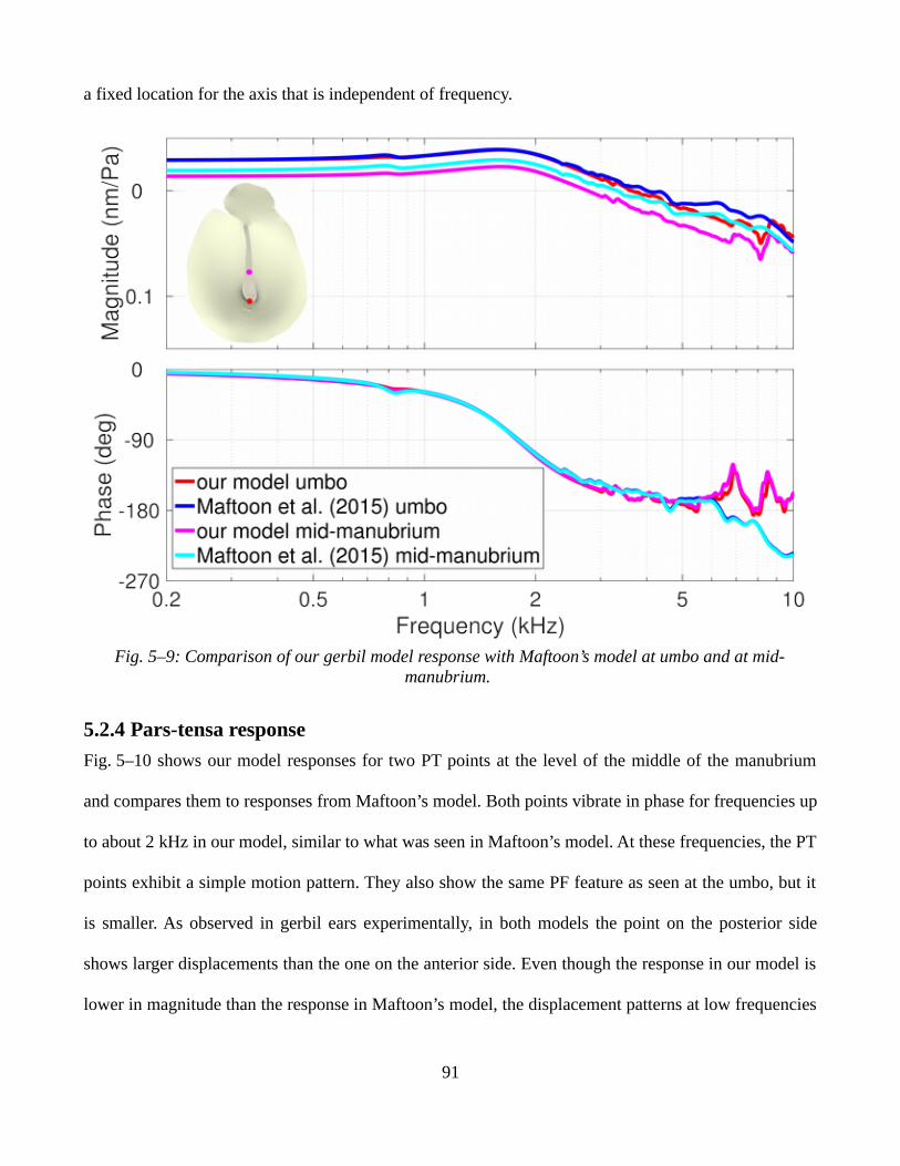
a fixed location for the axis that is independent of frequency.

Fig. 5–9: Comparison of our gerbil model response with Maftoon’s model at umbo and at mid-manubrium.

5.2.4 Pars-tensa response

Fig. 5–10 shows our model responses for two PT points at the level of the middle of the manubrium

and compares them to responses from Maftoon’s model. Both points vibrate in phase for frequencies up

to about 2 kHz in our model, similar to what was seen in Maftoon’s model. At these frequencies, the PT

points exhibit a simple motion pattern. They also show the same PF feature as seen at the umbo, but it

is smaller. As observed in gerbil ears experimentally, in both models the point on the posterior side

shows larger displacements than the one on the anterior side. Even though the response in our model is

lower in magnitude than the response in Maftoon’s model, the displacement patterns at low frequencies

91

are within the range of the patterns observed experimentally. The PT in our model is somewhat stiffer

than the one in Maftoon’s model due to its uniform thickness and our corresponding choice of material

properties.

The resonance has a similar shape in both models. The simple in-phase motion breaks up at higher

frequencies, with each point showing different frequency-dependent magnitudes and phases. As done

by Maftoon et al. (2013), we define the break-up frequency as the frequency at which the phase

divergence of the points on the PT is more than 15°. The break-up frequency for the PT points in our

model is 2.9 kHz. This is higher than the 2.2 kHz seen in Maftoon’s model (consistent with the higher

stiffness of our PT) but still close to the range of 1.8 to 2.8 kHz observed experimentally. The PT

magnitude responses from our model are within the range seen in the experimental responses (Maftoon

et al. 2014).

Figs. 5–5 and 5–10 indicate that the shunting of low frequencies by our PF and its effect on umbo

and PT is less than in Maftoon’s model. This effect of the PF is strongly affected by the size of the

middle-ear cavity (e.g., Rosowski et al., 1997; Maftoon et al., 2014). Smaller cavity sizes result in a

stronger effect of the PF on the response of the umbo and PT. Thus, with an open middle-ear cavity, the

PF has a very small effects on the motion of the PT and umbo, as seen in our model and Maftoon’s

model. In the open-cavity configuration, the effect may be strongly modulated by the coupling of the

PF with the manubrium and PT. The PT thickness in Maftoon’s model was variable, while in our case it

has a constant thickness of 15.8 µm, and this thickness along with the defined material properties

resulted in a stiffer PT in our model. This could affect the coupling between PT and PF, making the

effect of the PF on the PT much smaller. Furthermore, the coupling between manubrium and PT is

affected by the position of the axis of rotation, which is different than in Maftoon’s model. This also

might alter the effect of the PF on the umbo. Such speculations about the coupling between different

structures of the middle ear could be verified by modelling different configurations: changing the axis

92

of rotation, varying the PT thickness and material properties, etc.

Fig. 5–10: Comparison of our gerbil model response with Maftoon’s model (2015) response at a pointin anterior PT and a point in posterior PT

5.3 Pressurized vibrations

5.3.1 Triangular quasi-static pressure signals

5.3.1.1 Displacement versus quasi-static pressure

In this section we report the response of our model to slowly varying triangular pressure waves with

amplitude ±2.5 kPa and linear pressure-change rates between 200 Pa/s and 1.5 kPa/s, as was measured

experimentally at the umbo in the rabbit middle ear by Dirckx et al. (2006). The cochlear damping was

not included in the model. As some of the components of our gerbil middle-ear model are viscoelastic,

repeated pressurization cycles can give different results. To obtain stable responses, we simulated the

motion of different points on the TM and manurbrium at all pressure-change rates for about 5 to 6

93

cycles and examined how the response varied from one cycle to another. Fig. 5–11A shows umbo

displacement at 200 Pa/s as a function of pressure for 6 cycles. No significant change in the umbo

displacement is seen after the first cycle. Overall, the changes during the preconditioning were very

small for this low rate of pressure change and the curves nearly coincide, which was also clearly

observed in the measurements by Dirckx et al. This was also the case for the other pressure-change

rates. For subsequent simulations in this section, we report the displacement results of the third cycle.

Fig. 5–12 shows the simulated displacement of a point on the anterior PT. Near 0 Pa pressure, some

local buckling happens, as highlighted by circles in the figure. The instability of the TM is manifested

by sharp ‘kinks’ as shown in Fig. 5–12A. Each kink has a local minimum followed by a local

maximum in the ascending branch and vice versa in the descending branch. The inflection point at the

94

Fig. 5–11: Simulated umbo response to about 6 cycles of triangular waves of pressure for a pressure-change rate of 200 Pa/s. A: Umbo displacement as a function of time. B: Umbo displacement as a

function of pressure for all cycles.

middle of the kink is at about 150 Pa pressure in the ascending branch and about 300 Pa in the

descending branch. In Fig. 5–12B, the buckling is manifested as a transient decrease of the

displacement as pressure increases during loading, and as a transient increase of the displacement as the

pressure decreases during unloading. At positive pressures, the anterior PT flips over from a slightly

convex shape to a slightly concave shape during loading (and vice versa during unloading), without

ever becoming perfectly flat. This instability, with the TM jumping from one equilibrium configuration

to a very different equilibrium configuration, has been reported experimentally by other groups as well

(e.g., Dirckx et al., 1998; Ladak et al., 2004), but never simulated to the best of our knowledge. In this

pressure range, very fine time steps are required for numerical convergence. It becomes even more

challenging to model as the degree of buckling increases.

Fig. 5–12: Simulated anterior PT response to about 6 cycles of triangular waves of pressure for apressure-change rate of 200 Pa/s. A:Displacement as a function of time. B: Displacement as a function

of pressure for all cycles. Circles highlight some regions of buckling. C: Magnified view of the leftcircle in A. D: Magnified view of the right circle in A.

Fig. 5–13A shows our simulated umbo motion for different linear pressure-change rates ranging from

95

200 Pa/s to 1500 Pa/s (corresponding to frequencies ranging from 20 mHz to 150 mHz). We see that

the umbo motion is strongly nonlinear. For pressures beyond +1 kPa, for all frequencies the changes of

the umbo displacement are relatively small. For pressures beyond –1 kPa, however, the slope for

displacement versus pressure is still quite steep. Fig. 5–13B shows the experimental umbo motions

measured by Dirckx et al. (2006) for the rabbit middle ear for different pressure-change rates. The axis

have been reversed horizontally and vertically from what was presented in their paper because their

pressures were applied in the middle-ear cavity rather than on the ear-canal side of the TM as in our

model. The experimental displacement curves are very different from ours. Dirckx et al. (2006)

reported that umbo displacement changes by only a few micrometers beyond ±2 kPa in the rabbit

middle-ear. They observed that at these high pressures a wrinkle appeared in the TM around the umbo

and the umbo displacement decreased slightly as the pressure magnitude continued to increase,

especially at low pressure-change rates. This effect in the rabbit middle ear was not seen for our model

of the gerbil middle ear.

From Fig. 5–13A we can see that amplitudes at negative ear-canal pressures are always significantly

larger than amplitudes at equal positive pressures. This asymmetry is less pronounced but still present

in the rabbit as shown in Fig. 5–13B. We calculated the ratio of the maximal amplitudes at +2.5 and

−2.5 kPa for all pressure-change rates. For our model, the ratio of maximal displacement amplitudes

changed from 4.72 at 200 Pa/s to 4.69 at 1500 Pa/s, while in the rabbit experiment the ratio changed

from 2.21 at 200 Pa/s to 2.45 at 1500 Pa/s. In both cases the change was quite small. The actual ratios,

however, were smaller for the experimental rabbit data: averaged over pressure-change rates, the ratio

is 4.72 for the simulated gerbil umbo displacement but only 2.34 for the measured rabbit umbo

displacement. The displacements themselves were also smaller for the rabbit: the model umbo

peak-to-peak displacement at 200 Pa/s is 790 µm, compared with an umbo displacement of 165 µm at

the same pressure-change rate for the rabbit.

96

Fig. 5–13: Umbo displacement vs. pressure for various pressure-change rates. A: Model umbodisplacement. B: Experimental umbo displacement (Dirckx et al., 2006).C: Magnified view of panel A

from −2.0 kPa to −2.5 kPa. D: Magnified view of panel A from +2.0 kPa to +2.5 kPa.

97

Figs. 5–13C and 5–13D show magnified views of the two rectangles in Fig. 5–14A, to show how the

model umbo displacement varies as a function of pressure-change rate at −2.5 kPa and +2.5 kPa. We

see that increasing the pressure-change rate makes the umbo displacement slightly less negative at

−2.5 kPa and slightly less positive at +2.5 kPa. Thus, the simulated gerbil peak-to-peak umbo

displacement decreases slightly as a function of increasing pressure-change rate: it changed from

790 µm at 200 Pa/s to 776 µm at 1.5 kPa/s. Dirckx et al. (2006) reported a dependence of the

peak-to-peak umbo displacement on the pressure-change rate that was in the same direction but much

more pronounced, decreasing from 165 µm (SD=19) at 200 Pa/s to 118 µm (SD=15) at 1.5 kPa/s,for 10

rabbits.

Fig. 5–13A shows approximately the same amount of hysteresis at all pressure-change rates. On the

other hand, the experimental measurements on the rabbit middle ear in Fig. 5–13B show a hysteresis

that decreases with increasing pressure-change rate: at 200 Pa/s the hysteresis, computed as the surface

area enclosed by the displacement vs. pressure curve, is more than double the hysteresis at 1.5 kPa/s.

To evaluate the effects of the Prony series parameters on hysteresis, we increased (one at a time) the

coefficient of each of the six time constants of the PT (see section 4.4.12), manubrium and wedge from

0.07 to 0.6 while keeping all other parameters the same. This increase in the Prony-series coefficients

still satisfies the constraint that the sum of the coefficients should be less than 1 (refer to

section 3.3.2.3). Fig. 5–14 shows the hysteresis at pressure-change rates ranging from 0.2 Pa/s to

1.5 kPa/s when the coefficient for time constant 2.3 s (corresponding to ≈70 mHz or 700 Pa/s) has been

increased from 0.07 to 0.6. This will be referred to as gerbil model 2 while the original model is

referred to as gerbil model 1. Fig. 5–14 shows that the hysteresis in gerbil model 2 is much greater than

that in gerbil model 1 (Fig. 5–13A). In Fig. 5–14, the most hysteresis is observed at 30 mHz (300 Pa/s),

with slightly less at 200 Pa/s, and the smallest hysteresis is obtained with 150 mHz (1500 Pa/s). For

pressure-change rates 300 Pa/s, 500 Pa/s, 1000 Pa/s and 1500 Pa/s, a complete closed loop for

98

hysteresis could not be obtained because the FE solver failed to converge in the buckling region.

Increasing the coefficient of the Prony series to a very high value leads to a more pronounced

instability on the PT.

Fig. 5–14: Model umbo displacement as function of pressure at different ultra-low frequencies whenthe coefficient of the time constant 2.3 s is increased from 0.07 to 0.6.

To compare the hysteresis in the two models and with experimental measurements, the usual measure

would be the surface area enclosed by the displacement-versus-pressure curve. However, since for

gerbil model 2 the curves do not form a closed loop, we decided to measure the displacement

difference between the loading and unloading curves at −1000 Pa, where the hysteresis is most

pronounced for all models. Fig. 5–15 shows the displacement difference for both of our gerbil models

and for the rabbit experimental measurements of (Dirckx et al., 2006). The amount of hysteresis

remains almost unchanged for all pressure-change rates for gerbil model 1, in which the coefficients of

99

the Prony series are the same in PT, manubrium and wedge. The amount of hysteresis in model 1 is

very similar to that in the experimental data at pressure-change rates of 0.5, 1.0 and 1.5 kPa/s. At lower

rates (300 and 200 Pa/s) the experimental hysteresis increases by 20 to 25% while the model hysteresis

decreases slightly. For model 2, we were able to obtain hysteresis measures for only three

pressure-change rates: 200 Pa/s, 300 Pa/s and 1500 Pa/s. The amount of hysteresis is about five times

higher than for model 1 and the experimental data. The most hysteresis in the model is obtained with a

pressure-change rate of 300 Pa/s; there is about the same amount (11% less) at 200 Pa/s and much less

(34% less) at 1500 Pa/s. The trends are similar for the experimental data, with a small change (an

increase of 7%) from 300 Pa/s to 200 Pa/s and a large reduction (52%) from 300 Pa/s to 1500 Pa/s.

This modelling shows that, by changing the viscoelastic parameters, we can control the amount of

hysteresis at different frequencies. On the one hand, in gerbil model 1 where the coefficients of the

Prony series are equal, hysteresis was almost constant for all pressure-change rates. On the other hand,

in gerbil model 2 where the Prony-series coefficient corresponding to a frequency of 70 mHz

(corresponding to a pressure-change rate of 700 Pa/s) was greater than for the other coefficients,

hysteresis at the nearby pressure-change rates (30 mHz and 300 Pa/s) increased the most. Although we

could not measure the hysteresis at 500 Pa/s (50 mHz) and 1000 Pa/s (1000 mHz), we expect that the

hysteresis at 500 Pa/s would be even greater than the hysteresis at 300 Pa/s. When we change the

coefficients for time constants 10 µs (≈16 kHz), 220 µs (≈724 Hz), 5 ms (≈32 Hz), 110 ms (≈15 Hz)

and 52 s (≈3 mHz), outside the range of time constants corresponding to the pressure-change rates 300

to 1500 Pa/s (20 mHz to 150 mHz), the model hysteresis remains unchanged.

100

Fig. 5–15: Umbo hysteresis as a function of pressure-change rate, measured in the two gerbil modelsand in the experiment by Dirckx et al. (2006).

Motallebzadeh et al. (2013) computed the lost-energy spectra (using the method described by

Charlebois et al. (2013)) for one-term, two-term and three-term Prony series to study the individual

effect of each time constant and its corresponding coefficient. They found that each term has a peak at

an angular frequency corresponding to the inverse of its time constant. The height of each peak depends

on the value of the associated coefficient. The influence of each term spans about one decade before

and one decade after its peak with decreasing effect. Thus, in model 2, it makes sense to see that

changing the coefficient of the time constant corresponding to the frequency 70 mHz affects all

pressure-change rates (20-150 mHz), and that the effect gets smaller as we move further from that

frequency.

101

5.3.1.2 Vibration amplitude versus quasi-static pressure

To relate the results we obtained in section 5.2.1.1 to tympanometry, with our gerbil model 1 we apply

a pure tone of 226 Hz for 300 ms around zero pressure on both the ascending and descending branches

of the pressure sweep with a pressure-change rate of 1500 Pa/s. The acoustical stimulus of ±1 Pa

amplitude (equivalent to 94 dB SPL) is first applied from 6.53 s to 6.83 s, to cover a range of static

pressure from −225 Pa to +225 Pa. It is then also applied from 9.91 s to 10.21 s, to cover a range of

static pressure from +165 Pa and −285 Pa. The acoustic stimulus was applied for these two short

periods, instead of for the entire loading and unloading branches as done in tympanometry, to reduce

the computation time. In both cases we pass through zero static pressure. Fig. 5–16A shows the umbo

displacement as a function of time in response to the quasi-static pressure and sound stimulus.

Fig. 5–16B is a magnified view of the left rectangle in Fig. 5–16A and shows the small displacements

resulting from the application of the pure tone during the ascending branch.

Fig. 5–17 shows the resulting umbo acoustical response with the quasi-static response subtracted away.

102

Fig. 5–16: Response of the model to a 226-Hz pure tone during large sweeps of quasi-static pressure.A: Model umbo displacement as function of time. Rectangles indicate areas where the acoustic

stimulus was applied. B: Magnified view of the left square in A to highlight the acoustic induceddisplacements during the ascending branch. Arrows indicate the start and end of the vibrations.

As seen in Fig. 5–17A for the ascending branch, as the static pressure increases, the umbo vibration

increases slightly, then starting at time 6.66 s (corresponding to a quasi-static pressure of –28.6 Pa) it

decreases. For the descending branch (Fig. 5–17B), as the static pressure decreases the umbo vibration

increases, and then starting at time 10.067 s (corresponding to a quasi-static pressure of –70.5 Pa) it

decreases slightly. At the onset of the acoustic stimulus in panel A, pronounced transient effects are

observed for the first three cycles. This phenomenon is only observed for the ascending pressure; this

could be due to the fact that, at the onset of the tone on the ascending branch, the acoustical pressure is

moving in the opposite direction as the static-pressure sweep, while it is moving in the same direction

on the descending branch.

We also observe in both panels that the vibration amplitude appears to be modulated with a period of

4 to 6 cycles. It is not clear what the origin of this modulation is. It may be a consequence of

(1) complex interactions between the viscoelastic effects of some components of our model (which are

expressed in terms of six different time constants corresponding to frequencies ranging from 3 mHz

to16 kHz) with the frequencies of the pressure signals; or (2) the numerical integration in the FE solver.

Fig. 5–18 shows a magnified view of the vibration in the descending branch from 10.01 s to 10.06 s.

We can see some irregularities in the vibration, starting from 10.025 s (quasi-static pressure of 7.5 Pa)

and continuing up to around 10.04 s (quasi-static pressure of 30 Pa). We believe that these irregularities

in the vibrations are a consequence of buckling (as described in section 5.3.1.1) since they manifest

during loading and unloading at positive pressures near 0 Pa.

103

Fig. 5–17: Model umbo vibration after removing the displacement induced by quasi-static pressuresweep. A: Umbo vibration in the ascending branch. B: Umbo vibration in the descending branch.

104

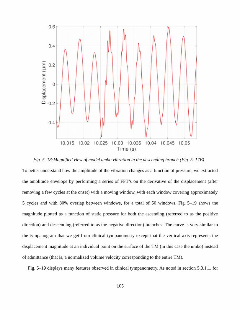
Fig. 5–18:Magnified view of model umbo vibration in the descending branch (Fig. 5–17B).

To better understand how the amplitude of the vibration changes as a function of pressure, we extracted

the amplitude envelope by performing a series of FFT’s on the derivative of the displacement (after

removing a few cycles at the onset) with a moving window, with each window covering approximately

5 cycles and with 80% overlap between windows, for a total of 50 windows. Fig. 5–19 shows the

magnitude plotted as a function of static pressure for both the ascending (referred to as the positive

direction) and descending (referred to as the negative direction) branches. The curve is very similar to

the tympanogram that we get from clinical tympanometry except that the vertical axis represents the

displacement magnitude at an individual point on the surface of the TM (in this case the umbo) instead

of admittance (that is, a normalized volume velocity corresponding to the entire TM).

Fig. 5–19 displays many features observed in clinical tympanometry. As noted in section 5.3.1.1, for

105

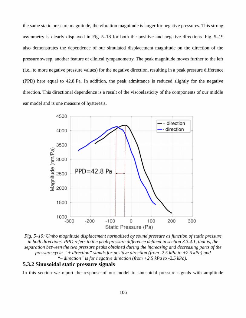
the same static pressure magnitude, the vibration magnitude is larger for negative pressures. This strong

asymmetry is clearly displayed in Fig. 5–18 for both the positive and negative directions. Fig. 5–19

also demonstrates the dependence of our simulated displacement magnitude on the direction of the

pressure sweep, another feature of clinical tympanometry. The peak magnitude moves further to the left

(i.e., to more negative pressure values) for the negative direction, resulting in a peak pressure difference

(PPD) here equal to 42.8 Pa. In addition, the peak admittance is reduced slightly for the negative

direction. This directional dependence is a result of the viscoelasticity of the components of our middle

ear model and is one measure of hysteresis.

5.3.2 Sinusoidal static pressure signals

In this section we report the response of our model to sinusoidal pressure signals with amplitude

106

Fig. 5–19: Umbo magnitude displacement normalized by sound pressure as function of static pressurein both directions. PPD refers to the peak pressure difference defined in section 3.3.4.1, that is, the

separation between the two pressure peaks obtained during the increasing and decreasing parts of thepressure cycle. “+ direction” stands for positive direction (from -2.5 kPa to +2.5 kPa) and

“– direction” is for negative direction (from +2.5 kPa to -2.5 kPa).

±1 kPa and frequencies 0.5 Hz, 5 Hz, 10 Hz and 50 Hz, as was performed experimentally in gerbil and

rabbit middle ears by Salih et al. (2016). In both model and experiment, pressure is applied to the

middle-ear cavity, so that positive pressures are associated with outward motion of the TM. This is

opposite to our model definition in section 5.3.1. Thus, the axis have been reversed horizontally (i.e.,

pressure) and vertically (i.e., displacement) for our simulations in this section.

The displacement amplitudes of our gerbil umbo as functions of pressure are presented in Fig. 5–20

and are compared with the displacement measured experimentally in 6 gerbils (Salih et al. 2016). The

model responses are quite similar to the experimental responses except at high positive pressures

greater than 800 Pa. Displacement at positive pressures fails to reach a plateau. At −1 kPa, the average

simulated umbo displacement is –97 µm for all frequencies, very similar to the -98 µm (SD=8) found

for all frequencies and gerbils for the experimental results. At +1 kPa, the average umbo displacement

is 351 µm for all frequencies, somewhat larger than the 286 µm (SD=35) for all frequencies and gerbils

experimentally. Thus, we again find the asymmetry seen in previous studies (e.g., Dirckx and

Decraemer, 2001; Dirckx et al., 2006). The simulated mean peak-to-peak displacement (i.e.,

displacement at +2.5 kPa minus displacement at −2.5 kPa) is equal to 448 μm (SD=10), compared with

an experimental value of 428 μm (SD=26). Overall, the model displacement values are well within the

range of experimental values.

107

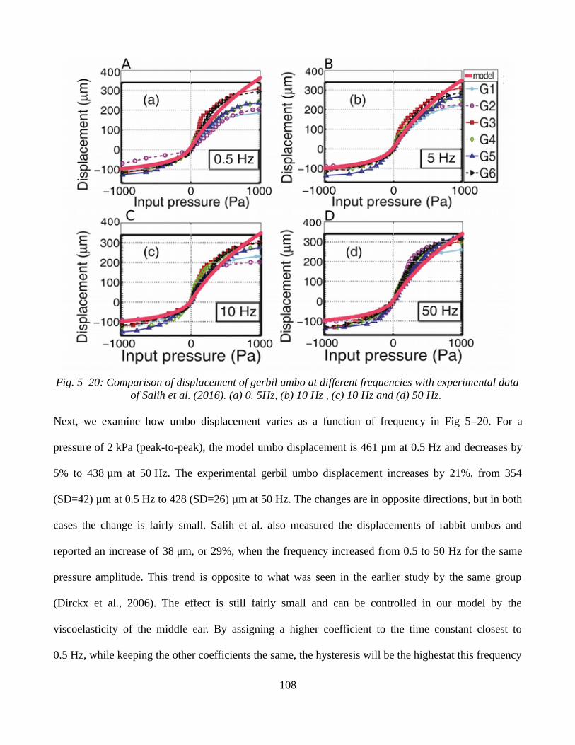
Fig. 5–20: Comparison of displacement of gerbil umbo at different frequencies with experimental dataof Salih et al. (2016). (a) 0. 5Hz, (b) 10 Hz , (c) 10 Hz and (d) 50 Hz.

Next, we examine how umbo displacement varies as a function of frequency in Fig 5–20. For a

pressure of 2 kPa (peak-to-peak), the model umbo displacement is 461 µm at 0.5 Hz and decreases by

5% to 438 µm at 50 Hz. The experimental gerbil umbo displacement increases by 21%, from 354

(SD=42) µm at 0.5 Hz to 428 (SD=26) µm at 50 Hz. The changes are in opposite directions, but in both

cases the change is fairly small. Salih et al. also measured the displacements of rabbit umbos and

reported an increase of 38 μm, or 29%, when the frequency increased from 0.5 to 50 Hz for the same

pressure amplitude. This trend is opposite to what was seen in the earlier study by the same group

(Dirckx et al., 2006). The effect is still fairly small and can be controlled in our model by the

viscoelasticity of the middle ear. By assigning a higher coefficient to the time constant closest to

0.5 Hz, while keeping the other coefficients the same, the hysteresis will be the highestat this frequency

108

and will decrease with increasing frequency while the umbo peak-to-peak displacement will be

smallest at this frequency and will increase with increasing frequencies.

Salih et al. (2016) reported an average umbo peak-to-peak displacement of 175 μm (SD=45) at

0.5 Hz for rabbits, compared with 354 μm (SD=42) at 0.5 Hz for gerbils. This corresponds to a ratio of

peak-to-peak displacement in gerbil to that in rabbit equal to about 2 for 0.5 Hz. In section 5.3.1.1, we

reported an umbo peak-to-peak displacement equal to 776 µm at 1500 Pa/s (150 mHz) in our gerbil

middle-ear model, compared with an experimental peak-to-peak rabbit umbo displacement of 118 μm

(SD=15) at 1500 Pa/s (Dirckx et al., 2006) which translates into a ratio of the peak-to-peak

displacement in gerbil to that in rabbit of 6.6. This ratio decreases with frequency and is equal to 4.7 at

200 Pa/s (20 mHz). The two sets of experiments (Dirckx et al. 2006 and Salih et al. 2016) cover quite

different frequency ranges (20 mHz-150 mHz vs. 0.5-50 Hz) and employ different pressure signals

(triangular vs. sinusoidal). It is thus not unexpected that the estimated ratio of the umbo peak-to-peak

displacement in gerbil to that in rabbit (6.6 at 150 mHz) would be different than the ratio measured by

Salih et al. (2 at 500 mHz).

5.3.3 Ramp static pressure signals combined with low-amplitude sound pressures

In this section we report the response of our model to a quasi-static pressure that is linearly increased

from zero to 250 Pa in 10 ms and then maintained at a constant value. After 15 ms a 50-ms acoustic

stimulus is superimposed on it, either a pure tone with a frequency of 226 Hz (Fig. 5–21 A & B) or a

chirp with constant amplitude and a linear frequency ramp from 0.12 to 3 kHz (Fig. 5–22 A & B). The

umbo displacements as function of time are shown in panels C and D of Figs. 5–21 and 5–22.

109

Fig. 5–21:Results for a quasi-static pressure combined with a 226-Hz pure tone using FEBio andCode_Aster. A: Input pressure signal. B. Magnified view corresponding to the rectangle in A to

show the acoustic stimulus. C: Umbo displacement as a function of time. D: Magnified viewcorresponding to the rectangle in C.

In Figs. 5–21C and 5–21D, we see that the umbo displacement increases nonlinearly as the static

pressure increases linearly for the first 10 ms. The nature of the nonlinearity is very similar in both

Code_Aster and FEBio, and the difference in displacement is less than 2%. Then, when the pressure

stays constant at 250 Pa, the displacement has a slight curvature with displacement increasing from

52.2 µm at 10 ms to 52.9 µm at 25 ms in FEBio. For Code_Aster, the displacement increases from

53.2 µm at 10 ms to 54 µm at 25 ms, corresponding to an increase of 0.8 µm compared with 0.7 µm in

FEBio. Both solvers show a behaviour typical of stress relaxation due to the viscoelasticity of the

system. The displacement resulting from the sinusoidal acoustical stimulus is very close to being a pure

sine wave of the same frequency riding on top of the slowly increasing response to the constant

pressure in both FEBio and Code_Aster. Aside from the transient effects seen at the onset, the

110

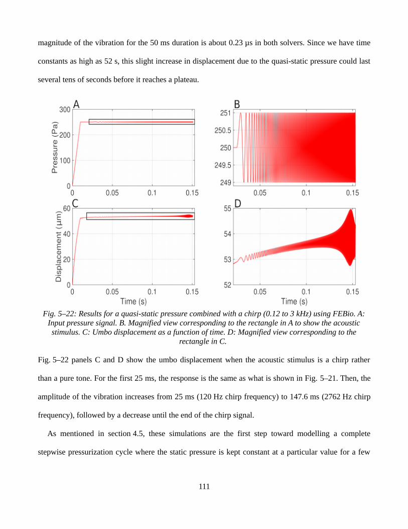
magnitude of the vibration for the 50 ms duration is about 0.23 µs in both solvers. Since we have time

constants as high as 52 s, this slight increase in displacement due to the quasi-static pressure could last

several tens of seconds before it reaches a plateau.

Fig. 5–22: Results for a quasi-static pressure combined with a chirp (0.12 to 3 kHz) using FEBio. A:Input pressure signal. B. Magnified view corresponding to the rectangle in A to show the acousticstimulus. C: Umbo displacement as a function of time. D: Magnified view corresponding to the

rectangle in C.

Fig. 5–22 panels C and D show the umbo displacement when the acoustic stimulus is a chirp rather

than a pure tone. For the first 25 ms, the response is the same as what is shown in Fig. 5–21. Then, the

amplitude of the vibration increases from 25 ms (120 Hz chirp frequency) to 147.6 ms (2762 Hz chirp

frequency), followed by a decrease until the end of the chirp signal.

As mentioned in section 4.5, these simulations are the first step toward modelling a complete

stepwise pressurization cycle where the static pressure is kept constant at a particular value for a few

111

seconds while the acoustic stimulus is continuously applied on the eardrum, as done in our group using

LDV measurements (e.g., Shapiro, 2014; Kose et al., 2017). There are not yet any experimental data to

compare with the simulation results. The preliminary measurements by Shapiro (2014) and Kose et al.

(2017) employ a peristaltic pump that cannot yet achieve a pressure rise time as fast as 10 ms, which

prevents us from investigating the short-term viscoelastic effects.

Furthermore, a serious issue with such simulations is the computational cost. A time step of 10 µs

was required for a pure-tone acoustic stimulus. The preliminary simulations took about 5 hours in

FEBio and about 35 hours in Code_Aster. When the acoustic stimulus was a chirp, the simulations

lasted 12 hours in FEBio. We used 7500 time steps for the pure tone and 15800 time steps for the chirp

for a single quasi-static pressure value, and these numbers will rise quickly when we want to consider a

complete pressurization cycle and higher frequencies (8 or 10 kHz).

5.3.4 Discussion

Dirckx and Decraemer (2001) showed that quasi-static eardrum displacement remained the same before

and after removing the cochlea. For quasi-static displacements, the presence of the cochlear fluid does

not much impede the motion of the TM due to the high static compliance of the round window, and

little effect is to be expected. The impedance of the cochlea becomes important at acoustic frequencies.

Therefore, even though we removed the cochlear impedance in this model (as mentioned in section

5.3.1.1)to better represent the no-cochlea condition of the rabbit middle ear in the experiment of Dirckx

et al. (2006), we can still compare our simulations of umbo displacements to results obtained with

intact middle ears.

We simulated the buckling in the PT, but encountered numerical challenges when larger instabilities

were obtained with gerbil model 2. Currently, FEBio only supports the Newton-Raphson

time-marching scheme, which is not the most suitable method to simulate mechanical instabilities.

112

Code_Aster makes it possible to circumvent some of the numerical difficulties of simulating buckling

by employing the arc-length method (Crisfield, 1981) which is suitable for “soft” snap-backs. For more

“abrupt” snap-backs other methods exist but are not currently available in Code_Aster (e.g., Riks et al.,

1996; Hellweg & Crisfield, 1998).

For our gerbil model 1, we obtained an umbo peak-to-peak displacement equal to 783 µm averaged

across all pressure-change rates. Ladak et al. (2004) reported umbo peak-to-peak values in cat, which

were around 300 to 600 µm, while Dirckx and Decraemer (2001) reported peak-to-peak values in the

gerbil middle ear with drained cochlea of about 350 µm in the region inferior to the umbo. The

displacements in the region inferior to the umbo will be bigger than the displacement at the umbo.

Eardrum sizes are comparable between cat and rabbit, but are smaller in gerbil. Furthermore, the gerbil

and cat PTs are thinner than in rabbit and human. The annulus of the rabbit and gerbil PT resembles the

shape in humans more than the cat. The PF’s in gerbil and rabbit are much larger (relative to the PT)

than in either cat or human. In our model (as in tympanometry) we increase the pressure linearly from 0

to 2.5 kPa in seconds, whereas in the moiré measurements the pressure increase was stepwise, with

several minutes of time interval between steps. All of these differences make it difficult to compare our

model results with previous work.

The asymmetry in our pressure vs. displacement curves (Fig. 5–13A), with negative pressures

causing higher displacements, has been reported by other studies as well. Dirckx and Decraemer (2001)

also identified this asymmetry and concluded that TM deformation in response to negative pressure is

strongly influenced by ossicular mechanics, while at positive pressures the maximal motion of the TM

is mainly determined by the elasticity of the membrane itself. Ladak et al. (2004) attributed the

asymmetry partially to the conical shape of the TM: due to this shape, the TM can easily balloon at

positive pressure but is stretched at negative pressure.

For acoustic frequencies below 1 kHz, Rosowski (1994) calculated values of the acoustic stiffness of

113

the TM and ossicles on the basis of acoustic stiffness measurements of the total middle ear and

middle-ear air space, and found 360 Pa/mm3 in gerbil, 500 Pa/mm3 in rabbit and 170 Pa/mm3 in human.

Thus, in the low-frequency acoustic range, the rabbit ear was a factor of about 1.5 stiffer than the gerbil

and the gerbil was a factor of 2 stiffer than human. We found a peak-to-peak umbo displacement equal

to 790 µm in the gerbil at 200 Pa/s while Dirckx et al. (2006) measured a peak-to-peak umbo

displacement equal to 165 µm in the rabbit at 200 Pa/s, which is a factor of 4.8 less. Hüttenbrink (1988)

measured a peak-to-peak umbo displacement of 540 µm at 200 Pa/s for the human ear, which is factor

of 1.5 less than our peak-to-peak gerbil umbo displacement. These factors are different from those

computed from the data of Rosowski (1994). However, the Rosowski data cover audio frequencies as

opposed to the ultra-low quasi-static frequencieckx et al. (2006) conducted their experiments on post

mortem rabbits. Whether the differences in results are due to species differences, to differences in the

freshness of the tissue or to differences in experimental methods is unclear.s covered by our model and

by the experimental data of Dirckx et al. (2006) and Hüttenbrink (1988).

Dirckx et al. (2006) suggested that the hysteresis trend of their experimental data was not governed

by viscoelasticity and they proposed a mechanism involving static and dynamic friction. They

suggested that “friction can occur between the ossicles and the middle-ear walls and within the ossicle

joints, and that static friction effects take over as the pressure-change rate decreases”. It is not clear to

us where this friction might occur, nor why static friction would be pronounced at 200 Pa/s where the

eardrum is moving substantially. In any case, results from our gerbil models 1 and 2 indicate that

hysteresis variation as a function of pressure-change rate can be controlled by the viscoelasticity of the

system. It thus appears that the trend observed by Dirckx et al., of greater hysteresis at lower

pressure-change rates, could be a consequence of viscoelasticity of several components of the middle

ear and can be modelled numerically by adjusting the Prony series coefficients in appropriate ranges of

frequency.

114

Salih et al. (2016) measured the motion of both gerbil and rabbit middle ears in response to very

low-frequency sinusoidal variations of static pressure, for amplitudes of ±500 Pa and ±1000 Pa and for

frequencies ranging from 0.5 to 50 Hz. In both species, the umbo displacement as a function of

frequency increased, as opposed to what is seen in our model and to what was seen experimentally by

the same group (Dirckx et al., 2006). The two sets of experiments used different measurement

techniques, covered very different ranges of freckx et al. (2006) conducted their experiments on post

mortem rabbits. Whether the differences in results are due to species differences, to differences in the

freshness of the tissue or to differences in experimental methods is unclear.quencies and used different

pressure signals (triangular vs. sinusoidal). Whether this is enough to explain the different results is not

clear.

It is hard to determine whether the amount of hysteresis computed for gerbil model 1 (Fig. 5–15) is

comparable to what is actually measured in the gerbil middle ear, given the lack of experimental

measurements of hysteresis. The plots of Dirckx and Decraemer (2001) show hysteresis for the gerbil

but it was not quantified. From their figure (Fig. 3–6 in section 3.4.3 here), one can see, however, that

the hysteresis was considerably greater than the hysteresis that we observe with gerbil model 1

(Figs. 5–13A and 5–15) and close to the hysteresis obtained with model 2 (Figs. 5–14 and 5–15) at

1500 kPa/s. The results are not directly comparable because the quasi-static pressure cycles were

different (triangular signal of a few seconds vs. stepwise variation with durations of several minutes).

We found a PPD of 42.8 Pa (Fig. 5–19) for a pressure-change rate of 1000 Pa/s when simulating

umbo vibration in the presence of quasi-static pressure sweeps. Although we did not measure the

variation of the PPD as a function of pressure-change rate, we expect that it will remain constant in our

gerbil model 1. Therkildsen and Gaihede (2005) used a modern high-speed commercial tympanometer

and found that, for pumping speeds ranging from 500 Pa/s to 4000 Pa/s, a constant PPD of 120 Pa was

measured in human ears. They thus concluded that hysteresis is constant, at least for this range of

115

pressure-change rates. As discussed in section 5.3.1.1, however, in the rabbit measurements of Dirckx

et al. (2006) the umbo hysteresis was greater at lower pressure-change rates. We can obtain similar

changes by manipulating the Prony-series coefficients. Therkildsen and Gaihede (2005) performed

their measurements on live humans while Dirckx et al. (2006) conducted their experiments on post

mortem rabbits. Whether the differences in results are due to species differences, to differences in the

freshness of the tissue or to differences in experimental methods is unclear.

116

Chapter 6: Conclusion

6.1 SummaryIn this study, a FE model of the gerbil middle ear was developed to study its response under conditions

involved in both clinical and experimental tympanometry, namely, both large quasi-static pressures and

small audio-frequency pressures. We created a FE model of the gerbil middle-ear that included the TM,

the manubrium, and a simplified representation of the ossicular chain and cochlear load with two

components referred to as the wedge and block. A fixed axis of rotation, around which the manubrium

rotates as a rigid body, was defined. We used two different FE solvers, FEBio and Code_Aster, as a

verification technique.

A quasi-linear viscoelastic model was used to describe the viscoelastic behaviour of the middle ear.

The viscoelastic parameters were defined with six equally spaced Prony-series time constants covering

a frequency range of 3 mHz to 16 kHz, covering the range of pressure-change rates and the frequencies

of acoustical stimulation in tympanometry. Their coefficients were initially assumed to be equal and set

to a constant value of 0.07. The elastic response of the TM was described by the Mooney-Rivlin

hyperelastic model while the manubrium, wedge and block were modelled as isotropic elastic. The

elastic properties of the model components were determined by studying the small-amplitude frequency

response of the model and comparing it with the model of Maftoon et al. (2015). To match Maftoon’s

model for different locations on the TM and manubrium, the Prony-series coefficients of the PF were

adjusted. The cochlear load was modelled differently in FEBio and Code_Aster. In FEBio, the

coefficient of the lowest time constant (10 µs) for the manubrium and wedge were increased to a high

value; in Code_Aster, a dashpot perpendicular to the manubrium was used. The two models were

compared and produced very similar results. Overall, the small-amplitude frequency response of our

model matched Maftoon’s model for frequencies up to 3 kHz. At higher frequencies, larger differences

117

were seen due to the assumptions made in our model. The PT was somewhat stiffer in our model, and

the PF effect on PT and umbo responses was smaller, but still within the range of experimental

measurements (Maftoon et al., 2013, 2014).

For comparison with experimental data, we explored the response of our gerbil middle-ear model to

large quasi-static pressures, both triangular sweeps with ultra-low frequencies (as used by Dirckx et al.,

2006, for rabbits), and sinusoidal sweeps with near-acoustic-range frequencies (as used by Salih et al.,

2016, for both rabbits and gerbils). We reported umbo peak-to-peak displacement as a function of

frequency and also measured hysteresis as a function of the pressure-change rate in the ultra-low

frequency range. In response to the triangular signal sweeps, we observed asymmetry of the umbo

displacement as a function of pressure. This asymmetry was also reported by Dirckx et al. (2006).

Umbo displacements at positive pressures were similar to those by measured by Dirckx et al, while

umbo displacements at negative pressures were much larger in our model. This could at least partly be

because we are comparing results from two different species. The discrepancy could be corrected by

adjusting the material nonlinearity of our model represented by the Mooney-Rivlin coefficients.

Hysteresis in our initial model was small and constant as function of frequency, while Dirckx et al.

reported an increasing hysteresis with decreasing pressure change rate. We have demonstrated that, by

changing the coefficients of the time constants within the range of the low pressure-change rates, we

can increase hysteresis and also control its variation as a function of frequency.

Exploring the response of our model to pressure sweeps at different locations on the PT indicated

that we were able to simulate TM buckling. This instability is manifested by sharp local kinks at small

positive pressures and was present for both the loading and unloading of the TM.

In response to sinusoidal pressures, we found that our displacements are in good agreement with the

experimental data except that once again we may be overestimating the umbo displacement for

negative pressures in the ear canal. The umbo peak-to-peak displacement increased slightly as

118

frequency decreased while Salih et al. (2016) reported a slight decrease. This discrepancy also could be

reduced by adjusting the coefficient of the time constant that covers the range of frequencies of interest.

The model umbo response to low-frequency pure tones applied on top of pressure sweeps at a

pressure-change rate of 1.5 kPa/s was investigated. We reported the vibration magnitude as a function

of pressure for the loading and unloading directions, to relate our results to clinical tympanograms. The

simulated static-pressure-induced variations in displacement of the umbo have features in common

with human tympanograms, including (1) the asymmetrical effects of positive and negative pressures;

and (2) the peak pressure difference and the slight decrease in magnitude from the ascending branch to

the descending branch, both resulting from hysteresis.

Finally, we studied the response of our model to a rapid pressure increase followed by an acoustic

stimulus consisting of either a pure tone (226 Hz) or a chirp (0.12 to 3 kHz). We applied this loading

condition to test the capability of our model to simulate conditions similar to LDV experiments

performed in our lab that use a stepwise pressurization protocol adapted from earlier work. In response

to the pure tone, Code_Aster and FEBio gave similar results; the simulation for a chirp was only

performed in FEBio. For both types of acoustic stimulus, we saw that the viscoelasticity strongly

affects the TM vibrations.

6.2 Future workDespite continuing advances in FE software, the realistic simulation of the middle-ear response under

simultaneous quasi-static and acoustical stimulation continues to be challenging. One reason for this is

the wide range of possible choices that can be made during the definition of a model. Therefore, a

sensitivity analysis is essential to understand the relative influences of some of these choices on the

middle-ear mechanisms under different loading conditions. For example, we should explore the effects

of the material properties; the TM curvature, geometry and thickness; the position of the axis of

119

rotation; and the boundary conditions

The generalized Maxwell viscoelastic model coupled with the Mooney-Rivlin hyperelastic model is

quasi-linear and may not reflect the intrinsic mechanical properties of the TM. The value of the viscous

modulus and its variation as a function of frequency are both controlled by the same parameters (gi and

τi). However, actual soft tissues exhibit strong non-inear viscoelasticity as clearly shown in Figs. 5–13B

and 5–14 in section 5.3.1.1 for the TM. For a more accurate representation of the mechanical behaviour

of soft tissues, a nonlinear viscohyperelastic model could be employed (Charlebois et al., 2013). It

introduces an additional parameter which allows seperate control of the variations of damping and

stiffness as functions of frequency.

The present model includes oversimplifications, and further improvements of the model can be

made by including the ear canal, annulus, ossicles, ligaments and middle-ear cavity, and by taking into

account a realistic thickness map for PT and PF, the anisotropy and multiple layers of the TM, and the

nonlinear viscoelasticity of the ligaments. On the other hand, we realize that more sophisticated models

will require a significantly more computational power and larger effort for their calibration. Thus, to

enable the development of more complex models, we first need to explore tools to decrease the

computational cost of our current model. Each stage of FE modelling (pre-processing, solution and

post-processing) has an inherent parallelism. Here, we are interested in exploiting parallelism in the

solution step. We could first start by optimizing our computations in both Code_Aster and FEBio by

investigating where they spend time. For a large number of degrees of freedom and slow performance

in calculation of the element matrices, implementing parallel Code_Aster and FEBio in Guillimin can

speed up our computations. FEBio has an implementation of a parallel solver for shared memory that

has been used in this study to decrease computational cost, but does not have an implementation of a

distributed-memory solver. On the other hand, one shared-memory solver (MULTI_FRONT) and two

different distributed-memory solvers (MUMPS and PETSC, which are direct and iterative,

120

respectively) are available for parallel computations in Code_Aster. However, there may be no

significant reduction in computational cost using such parallelism with the large number of time steps

that we are dealing with in our dynamic simulations, in the absence of parallelism in time.

We could alsoexploit graphical processing units (GPUs)for the FE solvers. Some groups have

implemented an explicit dynamic framework for nonlinear FE analysis using GPU execution, and it has

been shown to be much faster than CPU execution (e.g., Taylor et al., 2009).

Modelling buckling is numerically challenging. We ran into convergence problems in regions of

buckling when we increased the coefficients of some of our time constants. Incorporating different

numerical schemes in FEBio, and testing the capabilities of Code_Aster for modelling such

instabilities, should permit better modelling of buckling. The TM exhibits little plasticity, and the

buckled deflections are small and buckling loads are below the yield stress. Therefore, linear models of

buckling would be sufficient to model buckling in the TM. Once we develop an appropriate approach

to model buckling, we can incorporate the ossicular joints and model them as nonlinear viscoelastic

structures as done by Soleimani and Funnell (2016). These joints may also be prone to buckling, and by

modelling them we would gain a better understanding of the physical instabilities in the middle ear.

Not many data are available for the mechanical properties of the components of the gerbil middle

ear. We established estimates of parameters based on comparison with a previously validated linear

model (Maftoon et al., 2015). This approach, however, does not provide good estimates of the

nonlinearity and viscoelasticty of the gerbil middle ear. However, our model with its baseline

parameters can be used to simulate the gerbil middle ear in response to different loading conditions and

compare the results with experimental measurements. We can then adjust our material properties based

on these comparisons. As a first attempt in this experimental direction, in another study in our lab,

Shapiro (2014) performed preliminary post mortem multiple-point measurements on the gerbil TM in

response to chirps in the presence of step-wise changes in static pressures similar to those used

121

previously in measurements of TM shape in the gerbil (e.g., Dirckx & Decraemer, 2001). Currently, our

group is extending this work to acquire in vivo measurements and to extend it to more measurement

points (Kose et al., 2017). The pressurization introduces nonlinearities, and testing with different

pressurization cycles and pumping speeds will allow us to characterize the viscoelastic behaviour of the

gerbil middle ear. Thus, we will be able to obtain more a realistic and accurate numerical model of the

gerbil middle ear.

6.3 SignificanceIn general, the results of our study provide insight into the features present in tympanometry in gerbils,

and by extension in clinical tympanometry. To the best of our knowledge, this is the first time that the

response of the middle ear to both quasi-static pressures and acoustic pressures has been modelled,

accounting for both nonlinearity and viscoelasticity. The model provides a tool to bridge the gap

between quasi-static and acoustic measurements, and to explain the complex interactions between

them, which will enhance our understanding of tympanometry. Although our model is for the gerbil

middle ear, the ultimate goal is to understand clinical tympanometry in humans, and particularly in

newborns. Part of the rationale for studying the gerbil is to build confidence in our ability to explain

and model the behaviour of the middle ear by comparing the model to existing and future

measurements that cannot be done in humans.

Our study indicates that we can model the middle ear for conditions similar to those in

tympanometry (i.e., acoustic stimulus in presence of large pressure sweeps) but more work is needed to

clarify the response of the TM to different pressurization protocols, different frequencies of the acoustic

stimulus, different forms of the acoustic stimulus (i.e., pure tones, chirps or clicks) as well as the roles

of hysteresis, preconditioning and other temporal effects. This will lead to a better understanding of

tympanometry in gerbils and eventually in human newborns.

122

References

Abdala, C., & Keefe, D. H. (2012). Morphological and functional ear development. Human Auditory

Development (pp. 19–59). Springer.

Aernouts, J., & Dirckx, J. J. J. (2011). Elastic characterization of the gerbil pars flaccida from in situ

inflation experiments. Biomechanics and Modeling in Mechanobiology, 10(5), 727–741.

Aernouts, J., & Dirckx, J. J. J. (2012). Static versus dynamic gerbil tympanic membrane elasticity:

derivation of the complex modulus. Biomechanics and Modeling in Mechanobiology, 11(6), 829–

840.

Aernouts, J., Soons, J. A., & Dirckx, J. J. (2010). Quantification of tympanic membrane elasticity

parameters from in situ point indentation measurements: validation and preliminary study. Hearing

Research, 263(1), 177–182.

Agache, P. G., Monneur, C., Leveque, J. L., & De Rigal, J. (1980). Mechanical properties and Young’s

modulus of human skin in vivo. Archives of Dermatological Research, 269(3), 221–232.

Akache, F., Funnell, W. R. J., & Daniel, S. J. (2007). An experimental study of tympanic membrane and

manubrium vibrations in rats. Audiology and Neurotology, 12(1), 49–58.

Alberti, P. W., & Jerger, J. F. (1974). Probe-tone frequency and the diagnostic value of tympanometry.

Archives of Otolaryngology, 99(3), 206–210.

André, K. D., Sanches, S. G. G., & Carvallo, R. M. M. (2012). Middle ear resonance in infants: age

effects. International Archives of Otorhinolaryngology, 16(3), 353–357.

Anson, B. J., & Donaldson, J. A. (1973). Surgical anatomy of the temporal bone and ear. WB Saunders

Company.

Bailey, B. J. (2001). Atlas of Head & Neck Surgery-Otolaryngology (Vol. 2). Lippincott Williams &

Wilkins.

von Békésy, G. (1941). Über die Messung der Schwingungsamplitude der Gehörknöcheln mittels einer

kapazitiven Sonde.

von Békésy, G., & Wever, E. G. (1960). Experiments in Hearing (Vol. 8). McGraw-Hill New York.

123

Belytschko, T., Liu, W. K., Moran, B., & Elkhodary, K. (2013). Nonlinear Finite Elements for

Continua and Structures. John wiley & sons.

Bonifasi-Lista, C., Lakez, S. P., Small, M. S., & Weiss, J. A. (2005). Viscoelastic properties of the

human medial collateral ligament under longitudinal, transverse and shear loading. Journal of

Orthopaedic Research, 23(1), 67–76.

Buunen, T. J. F., & Vlaming, M. S. M. G. (1981). Laser–Doppler velocity meter applied to tympanic

membrane vibrations in cat. The Journal of the Acoustical Society of America, 69(3), 744–750.

Buytaert, J. A. N., Salih, W. H. M., Dierick, M., Jacobs, P., & Dirckx, J. J. J. (2011). Realistic 3D

Computer Model of the Gerbil Middle Ear, Featuring Accurate Morphology of Bone and Soft

Tissue Structures. Journal of the Association for Research in Otolaryngology, 12(6), 681–696.

Calandruccio, L., Fitzgerald, T. S., & Prieve, B. A. (2006). Normative multifrequency tympanometry in

infants and toddlers. Journal of the American Academy of Audiology, 17(7), 470–480.

Charlebois, M., McKee, M. D., & Buschmann, M. D. (2004). Nonlinear tensile properties of bovine

articular cartilage and their variation with age and depth. Journal of Biomechanical Engineering,

126(2), 129–137.

Charlebois, M., Motallebzadeh, H., & Funnell, W. R. J. (2013). Visco-hyperelastic law for finite

deformations: a frequency analysis. Biomechanics and Modeling in Mechanobiology, 1–11.

Cheng, J. T., Aarnisalo, A. A., Harrington, E., Hernandez-Montes, M. del S., Furlong, C., Merchant, S.

N., & Rosowski, J. J. (2010). Motion of the surface of the human tympanic membrane measured

with stroboscopic holography. Hearing Research, 263(1–2), 66–77.

Cheng, T., Dai, C., & Gan, R. Z. (2007). Viscoelastic Properties of Human Tympanic Membrane.

Annals of Biomedical Engineering, 35(2), 305–314.

Cheng, T., & Gan, R. Z. (2008). Mechanical properties of anterior malleolar ligament from

experimental measurement and material modeling analysis. Biomechanics and Modeling in

Mechanobiology, 7(5), 387–394.

Chole, R. A., & Kodama, K. (1989). Comparative histology of the tympanic membrane and its

relationship to cholesteatoma. Annals of Otology, Rhinology & Laryngology, 98(10), 761–766.

124

Christensen, R. (2012). Theory of Viscoelasticity: An Introduction. Elsevier.

Ciambella, J., Paolone, A., & Vidoli, S. (2010). A comparison of nonlinear integral-based viscoelastic

models through compression tests on filled rubber. Mechanics of Materials, 42(10), 932–944.

Cifuentes, A. O., & Kalbag, A. (1992). A performance study of tetrahedral and hexahedral elements in

3-D finite element structural analysis. Finite Elements in Analysis and Design, 12(3), 313–318.

Cohen, Y. E., Bacon, C. K., & Saunders, J. C. (1992). Middle ear development III: morphometric

changes in the conducting apparatus of the Mongolian gerbil. Hearing Research, 62(2), 187–193.

Colletti, V. (1975). Methodologic observations on tympanometry with regard to the probe tone

frequency. Acta Oto-Laryngologica, 80(1–6), 54–60.

Crisfield, M. A. (1981). A fast incremental/iterative solution procedure that handles “snap-through.”

Computers & Structures, 13(1), 55–62.

Cull, P. (1989). The Sourcebook of Medical Illustration. Parthenon Publishing.

Dahmann, H. (1929). Zur Physiologie des Hörens; experimentelle Untersuchungen über die Mechanik

der Gehörknöchelchenkette, sowie über deren Verhalten auf Ton und Luftdruck. Z. Hals-Nasen-u

Ohrenheilk (Leipzig), 24, 462–498.

Dai, C., Cheng, T., Wood, M. W., & Gan, R. Z. (2007). Fixation and detachment of superior and

anterior malleolar ligaments in human middle ear: experiment and modeling. Hearing Research,

230(1), 24–33.

Daniel, S. J., Funnell, W. R. J., Zeitouni, A. G., Schloss, M. D., & Rappaport, J. (2001). Clinical

application of a finite-element model of the human middle ear. Journal of Otolaryngology-Head &

Neck Surgery, 30(6), 340.

Daphalapurkar, N. P., Dai, C., Gan, R. Z., & Lu, H. (2009). Characterization of the linearly viscoelastic

behavior of human tympanic membrane by nanoindentation. Journal of the Mechanical Behavior

of Biomedical Materials, 2(1), 82–92.

Decraemer, W. F., Creten, W. L., & Van Camp, K. J. (1984). Tympanometric middle-ear pressure

determination with two-component admittance meters. Scandinavian Audiology, 13(3), 165–172.

Decraemer, W. F., Dirckx, J. J. J., & Funnell, W. R. J. (2003). Three-dimensional modelling of the

125

middle-ear ossicular chain using a commercial high-resolution X-ray CT scanner. Journal of the

Association for Research in Otolaryngology, 4(2), 250–263.

Decraemer, W. F., Khanna, S. M., & Funnell, W. R. J. (1989). Interferometric measurement of the

amplitude and phase of tympanic membrane vibrations in cat. Hearing Research, 38(1), 1–17.

Decraemer, W. F., de La Rochefoucauld, O., Dong, W., Khanna, S. M., Dirckx, J. J. J., & Olson, E. S.

(2007). Scala vestibuli pressure and three-dimensional stapes velocity measured in direct

succession in gerbil. The Journal of the Acoustical Society of America, 121(5), 2774–2791.

Decraemer, W. F., Maes, M. A., & Vanhuyse, V. J. (1980). An elastic stress-strain relation for soft

biological tissues based on a structural model. Journal of Biomechanics, 13(6), 463–468.

Decraemer, W., Maftoon, N., Dirckx, J., & Funnell, W. R. J. (2011). The effects of the asymmetric

shape of the tympanic membrane on the asymmetry of ossicular displacements for positive and

negative static pressures. ARO Midwinter Meeting.

Delalleau, A., Josse, G., Lagarde, J.-M., Zahouani, H., & Bergheau, J.-M. (2008). A nonlinear elastic

behavior to identify the mechanical parameters of human skin in vivo. Skin Research and

Technology, 14(2), 152–164.

Dhatt, G., Touzot, G., & others. (2012). Finite Element Method. John Wiley & Sons.

Dirckx, J. J., Buytaert, J. A., & Decraemer, W. F. (2006). Quasi-static transfer function of the rabbit

middle ear‚ measured with a heterodyne interferometer with high-resolution position decoder.

Journal of the Association for Research in Otolaryngology, 7(4), 339–351.

Dirckx, J. J., & Decraemer, W. F. (1991). Human tympanic membrane deformation under static

pressure. Hearing Research, 51(1), 93–105.

Dirckx, J. J. J., & Decraemer, W. F. (2001). Effect of middle ear components on eardrum quasi-static

deformation. Hearing Research, 157(1–2), 124–137.

Dirckx, J. J. J., Decraemer, W. F., von Unge, M., & Larsson, C. (1997). Measurement and modeling of

boundary shape and surface deformation of the Mongolian gerbil pars flaccida. Hearing Research,

111(1), 153–164.

Dirckx, J. J. J., Decraemer, W. F., von Unge, M., & Larsson, C. (1998). Volume displacement of the

126

gerbil eardrum pars flaccida as a function of middle ear pressure. Hearing Research, 118(1–2), 35–

46.

Dirckx, J. J. J., Somers, T., Decraemer, W. F., Govaerts, P., & Offeciers, E. (2001). Continuous pressure

monitoring in the intact middle ear. Cholesteatoma and Ear Surgery, 41–47.

Dong, W., & Olson, E. S. (2006). Middle ear forward and reverse transmission in gerbil. Journal of

Neurophysiology, 95(5), 2951–2961.

Eby, T. L., & Nadol, J. B. (1986). Postnatal growth of the human temporal bone: Implications for

cochlear implants in children. Annals of Otology, Rhinology & Laryngology, 95(4), 356–364.

Elkhouri, N., Liu, H., & Funnell, W. R. J. (2006). Low-Frequency Finite-Element Modeling of the

Gerbil Middle Ear. Journal of the Association for Research in Otolaryngology, 7(4), 399–411.

Ellaham, N. N., Akache, F., Funnell, W. R., & Daniel, S. J. (2007). Experimental study of the effects of

drying on middle-ear vibrations in the gerbil. 30th Annual Conference Canadian Medical

Bioligical Engineering Society.

Elner, A., Ingelstedt, S., & Ivarsson, A. (1971). The elastic properties of the tympanic membrane

system. Acta Oto-Laryngologica, 72(1–6), 397–403.

Fay, J. P., Puria, S., & Steele, C. R. (2006). The discordant eardrum. Proceedings of the National

Academy of Sciences, 103(52), 19743–19748.

Fay, J., Puria, S., Decraemer, W. F., & Steele, C. (2005). Three approaches for estimating the elastic

modulus of the tympanic membrane. Journal of Biomechanics, 38(9), 1807–1815.

Feldman, A. S. (1976). Tympanometry—Procedures, Interpretations and Variables. Acoustic

impedance and admittance: The measurement of middle ear function.

Ferekidis, E., Vlachou, S., Douniadakis, D., Apostolopoulos, N., & Adamopoulos, G. (1999). Multiple-

frequency tympanometry in children with acute otitis media. Otolaryngology–Head and Neck

Surgery, 121(6), 797–801.

Ferreira, A., Gentil, F., & Tavares, J. M. R. (2014). Segmentation algorithms for ear image data towards

biomechanical studies. Computer Methods in Biomechanics and Biomedical Engineering, 17(8),

888–904.

127

Ferry, J. D. (1980). Viscoelastic Properties of Polymers. John Wiley & Sons.

Funasaka, S., Funai, H., & Kumakawa, K. (1984). Sweep-frequency tympanometry: Its development

and diagnostic value. Audiology, 23(4), 366–379.

Fung, Y. (2013). Biomechanics: mechanical properties of living tissues. Springer Science & Business

Media.

Fung, Y.-C. (1993). Mechanical properties and active remodeling of blood vessels. Biomechanics (pp.

321–391). Springer.

Funnell, W. R., Decraemer, W. F., & Khanna, S. M. (1987). On the damped frequency response of a

finite-element model of the cat eardrum. The Journal of the Acoustical Society of America, 81(6),

1851–1859.

Funnell, W. R. J. (1983). On the undamped natural frequencies and mode shapes of a finite‐element

model of the cat eardrum. The Journal of the Acoustical Society of America, 73(5), 1657–1661.

Funnell, W. R. J., & Decraemer, W. F. (1996). On the incorporation of moiré shape measurements in

finite‐element models of the cat eardrum. The Journal of the Acoustical Society of America,

100(2), 925–932.

Funnell, W. R. J., Decraemer, W. F., Von Unge, M., & Dirckx, J. J. J. (2000). Finite-element modelling

of the gerbil eardrum and middle ear. 23rd Association for Research in Otolaryngology (ARO)

MidWinter Meeting.

Funnell, W. R. J., & Laszlo, C. A. (1975). Modeling the eardrum as a doubly curved shell using the

finite-element method. The Journal of the Acoustical Society of America, 57(S1), S72–S72.

Funnell, W. R. J., & Laszlo, C. A. (1978). Modeling of the cat eardrum as a thin shell using the finite‐

element method. The Journal of the Acoustical Society of America, 63(5), 1461–1467.

Funnell, W. R. J., Maftoon, N., & Decraemer, W. F. (2012). Mechanics and modelling for the middle

ear, 3, 2013.

Funnell, W. R., & Laszlo, C. A. (1982). A critical review of experimental observations on eardrum

structure and function. Journal for Otorhinolaryngology and its Related Specialties, 44(4), 181–

205.

128

Gaihede, M. (1996). Tympanometric preconditioning of the tympanic membrane. Hearing Research,

102(1), 28–34.

Gan, R. Z., Sun, Q., Feng, B., & Wood, M. W. (2006). Acoustic–structural coupled finite element

analysis for sound transmission in human ear-pressure distributions. Medical Engineering &

Physics, 28(5), 395–404.

Gan, R. Z., & Wang, X. (2007). Multifield coupled finite element analysis for sound transmission in

otitis media with effusion. The Journal of the Acoustical Society of America, 122(6), 3527–3538.

Gea, S. L., Decraemer, W. F., Funnell, R. W., Dirckx, J. J., & Maier, H. (2010). Tympanic membrane

boundary deformations derived from static displacements observed with computerized tomography

in human and gerbil. Journal of the Association for Research in Otolaryngology, 11(1), 1–17.

Geerligs, M., Van Breemen, L., Peters, G., Ackermans, P., Baaijens, F., & Oomens, C. (2011). In vitro

indentation to determine the mechanical properties of epidermis. Journal of Biomechanics, 44(6),

1176–1181.

Geuzaine, C., & Remacle, J.-F. (2009). Gmsh: A 3-D finite element mesh generator with built-in pre-

and post-processing facilities. International Journal for Numerical Methods in Engineering,

79(11), 1309–1331.

Ghadarghadar, N., Agrawal, S. K., Samani, A., & Ladak, H. M. (2013). Estimation of the quasi-static

Young’s modulus of the eardrum using a pressurization technique. Computer Methods and

Programs in Biomedicine, 110(3), 231–239.

Glater, J. (2009). Efficacy of 1000 Hz tympanometry in infants birth to 4 months of age: A follow up

study (Capstone Project). Washington University School of Medicine.

Govindjee, S., & Reese, S. (1997). A Presentation and Comparison of Two Large Deformation

Viscoelasticity Models. Journal of Engineering Materials and Technology, 119(3), 251–255.

He, Z. (2012). Vibration measurements on the widely exposed gerbil eardrum (Master’s). McGill

University (Canada).

Hellweg, H.-B., & Crisfield, M. A. (1998). A new arc-length method for handling sharp snap-backs.

Computers & Structures, 66(5), 704–709.

129

Herrmann, L. R., & Peterson, F. E. (1968). A numerical procedure for viscoelastic stress analysis.

Seventh meeting of ICRPG mechanical behavior working group, Orlando, FL, CPIA Publication

(pp. 60–69).

Holte, L., Cavanaugh, R. M., & Margolis, R. H. (1990). Ear canal wall mobility and tympanometric

shape in young infants. The Journal of Pediatrics, 117(1), 77–80.

Holte, L., Margolish, R. H., & Cavanaugh, R. M. (1991). Developmental changes in multifrequency

tympanograms. Audiology, 30(1), 1–24.

Holzapfel, G. A. (2000). Nonlinear solid mechanics: a continuum approach for engineering. John

Wiley & Sons Ltd.

Homma, K., Shimizu, Y., Kim, N., Du, Y., & Puria, S. (2010). Effects of ear-canal pressurization on

middle-ear bone and air-conduction responses. Hearing Research, 263(1–2), 204–215.

Huang, G., Daphalapurkar, N. P., Gan, R. Z., & Lu, H. (2008). A method for measuring linearly

viscoelastic properties of human tympanic membrane using nanoindentation. Journal of

Biomechanical Engineering, 130(1), 014501-014501-7.

Huber, A. M., Schwab, C., Linder, T., Stoeckli, S. J., Ferrazzini, M., Dillier, N., & Fisch, U. (2001).

Evaluation of eardrum laser Doppler interferometry as a diagnostic tool. The Laryngoscope,

111(3), 501–507.

Humphrey, J. D. (2003). Continuum biomechanics of soft biological tissues. Proceedings of the Royal

Society of London A: Mathematical, Physical and Engineering Sciences (Vol. 459, pp. 3–46). The

Royal Society.

Hüttenbrink, K.-B. (1988). The mechanics of the middle-ear at static air pressures: the role of the

ossicular joints, the function of the middle-ear muscles and the behaviour of stapedial prostheses.

Acta Oto-Laryngologica, 105(sup451), 1–35.

Ikui, A., Sando, I., Haginomori, S.-I., & Sudo, M. (2000). Postnatal development of the tympanic

cavity: a computer-aided reconstruction and measurement study. Acta Oto-Laryngologica, 120(3),

375–379.

James, C. (2006, February 10). Finite element modeling and exploration of double hearing protection

130

systems (Master’s). Virginia Tech.

Jerger, J. (1970). Clinical experience with impedance audiometry. Archives of Otolaryngology, 92(4),

311–324.

Keefe, D. H., & Levi, E. (1996). Maturation of the middle and external ears: acoustic power-based

responses and reflectance tympanometry. Ear and Hearing, 17(5), 361–373.

Keefe, D. H., & Simmons, J. L. (2003). Energy transmittance predicts conductive hearing loss in older

children and adults. The Journal of the Acoustical Society of America, 114(6), 3217–3238.

Kei, J., Allison-Levick, J., Dockray, J., Harrys, R., Kirkegard, C., Wong, J., Maurer, M., et al. (2003).

High-frequency (1000 Hz) tympanometry in normal neonates. Journal of the American Academy

of Audiology, 14(1), 20–28.

Kelly, D. J., Prendergast, P. J., & Blayney, A. W. (2003). The effect of prosthesis design on vibration of

the reconstructed ossicular chain: a comparative finite element analysis of four prostheses. Otology

& Neurotology, 24(1), 11–19.

Kessel, J. (1874). On the influence of the middle-ear muscles on the displacements and vibrations of

the eardrum in the cadaver ear. Arch. OhrenhLk, 8, 80–92.

Khanna, S. M., & Tonndorf, J. (1972). Tympanic membrane vibrations in cats studied by time-averaged

holography. The Journal of the Acoustical Society of America, 51(6), 1904–1920.

Kilic, A., Baysal, E., Karatas, E., Baglam, T., Durucu, C., Deniz, M., & Mumbuc, S. (2012). The role of

high frequency tympanometry in newborn hearing screening programme. European Review for

Medical and Pharmacological Sciences, 16(2), 220–223.

Kim, N., Homma, K., & Puria, S. (2011). Inertial bone conduction: symmetric and anti-symmetric

components. Journal of the Association for Research in Otolaryngology, 12(3), 261–279.

Kirikae, I. (1960). The Structure and Function of the Middle Ear. University of Tokyo Press.

Knauss, W. G., & Zhao, J. (2007). Improved relaxation time coverage in ramp-strain histories.

Mechanics of Time-Dependent Materials, 11(3–4), 199–216.

Koike, T., Wada, H., & Kobayashi, T. (2002). Modeling of the human middle ear using the finite-

element method. The Journal of the Acoustical Society of America, 111(3), 1306–1317.

131

Konrádsson, K. S., Ivarsson, A., & Bank, G. (1987). Computerized laser Doppler interferometric

scanning of the vibrating tympanic membrane. Scandinavian Audiology, 16(3), 159–166.

Kose, O., Funnell, W. R. J., & Daniel, S. J. (2017). In vivo experimental study of gerbil eardrum

vibrations under static pressures. Presented at the 39th Association for Research in Otolaryngology

(ARO) MidWinter Meeting.

Kuijpers, W., Peters, T. A., & Tonnaer, E. L. (1999). Nature of the tympanic membrane insertion into

the tympanic bone of the rat. Hearing Research, 128(1–2), 80–88.

Kuypers, L. C., Decraemer, W. F., & Dirckx, J. J. (2006). Thickness distribution of fresh and preserved

human eardrums measured with confocal microscopy. Otology & Neurotology, 27(2), 256–264.

Kuypers, L. C., Dirckx, J. J., Decraemer, W. F., & Timmermans, J.-P. (2005). Thickness of the gerbil

tympanic membrane measured with confocal microscopy. Hearing Research, 209(1), 42–52.

de La Rochefoucauld, O., Decraemer, W. F., Khanna, S. M., & Olson, E. S. (2008). Simultaneous

measurements of ossicular velocity and intracochlear pressure leading to the cochlear input

impedance in gerbil. Journal of the Association for Research in Otolaryngology, 9(2), 161–177.

de La Rochefoucauld, O., & Olson, E. S. (2010). A sum of simple and complex motions on the eardrum

and manubrium in gerbil. Hearing Research, 263(1), 9–15.

Ladak, H. M., Decraemer, W. F., Dirckx, J. J. J., & Funnell, W. R. J. (2004). Response of the cat

eardrum to static pressures: Mobile versus immobile malleus. The Journal of the Acoustical

Society of America, 116(5), 3008–3021.

Ladak, H. M., & Funnell, W. R. J. (1996). Finite-element modeling of the normal and surgically

repaired cat middle ear. The Journal of the Acoustical Society of America, 100(2), 933–944.

Ladak, H. M., Funnell, W. R. J., Decraemer, W. F., & Dirckx, J. J. J. (2006). A geometrically nonlinear

finite-element model of the cat eardrum. The Journal of the Acoustical Society of America, 119(5),

2859–2868.

Landel, R. F., & Nielsen, L. E. (1993). Mechanical properties of polymers and composites. Crc Press.

Lee, C. Y., & Rosowski, J. J. (2001). Effects of middle-ear static pressure on pars tensa and pars

flaccida of gerbil ears. Hearing Research, 153(1–2), 146–163.

132

Lee, C.-F., Chen, P.-R., Lee, W.-J., Chen, J.-H., & Liu, T.-C. (2006). Three-dimensional reconstruction

and modeling of middle ear biomechanics by high-resolution computed tomography and finite

element analysis. The Laryngoscope, 116(5), 711–716.

Lesser, T. H. J., & Williams, K. R. (1988). The tympanic membrane in cross section: a finite element

analysis. The Journal of Laryngology & Otology, 102(3), 209–214.

Lim, D. J. (1968). Tympanic membrane part II: pars flaccida. Acta Oto-Laryngologica, 66(1–6), 515–

532.

Lim, D. J. (1970). Human tympanic membrane: an ultrastructural observation. Acta Oto-

Laryngologica, 70(3), 176–186.

Luo, H., Dai, C., Gan, R. Z., & Lu, H. (2009a). Measurement of Young’s modulus of human tympanic

membrane at high strain rates. Journal of Biomechanical Engineering, 131(6), 064501.

Luo, H., Lu, H., Dai, C., & Gan, R. Z. (2009b). A comparison of Young’s modulus for normal and

diseased human eardrums at high strain rates. International Journal of Experimental and

Computational Biomechanics, 1(1), 1–22.

Maftoon, N., Funnell, W. R. J., Daniel, S. J., & Decraemer, W. F. (2013). Experimental study of

vibrations of gerbil tympanic membrane with closed middle ear cavity. Journal of the Association

for Research in Otolaryngology, 14(4), 467–481.

Maftoon, N., Funnell, W. R. J., Daniel, S. J., & Decraemer, W. F. (2014). Effect of opening middle-ear

cavity on vibrations of gerbil tympanic membrane. Journal of the Association for Research in

Otolaryngology, 15(3), 319–334.

Maftoon, N., Funnell, W. R. J., Daniel, S. J., & Decraemer, W. F. (2015). Finite-element modelling of

the response of the gerbil middle ear to sound. Journal of the Association for Research in

Otolaryngology, 16(5), 547–567.

Manley, G. A., & Johnstone, B. M. (1974). Middle‐ear function in the guinea pig. The Journal of the

Acoustical Society of America, 56(2), 571–576.

Marchant, C. D., McMillan, P. M., Shurin, P. A., Johnson, C. E., Turczyk, V. A., Feinstein, J. C., &

Panek, D. M. (1986). Objective diagnosis of otitis media in early infancy by tympanometry and

133

ipsilateral acoustic reflex thresholds. The Journal of Pediatrics, 109(4), 590–595.

Martins, P. a. L. S., Natal Jorge, R. M., & Ferreira, A. J. M. (2006). A comparative study of several

material models for prediction of hyperelastic properties: application to silicone-rubber and soft

tissues. Strain, 42(3), 135–147.

McKinley, A. M., Grose, J. H., & Roush, J. (1997). Multifrequency tympanometry and evoked

otoacoustic emissions in neonates during the first 24 hours of life. Journal of the American

Academy of Audiology, 8(3).

McLellan, M. S., & Webb, C. H. (1957). Ear studies in the newborn infant: natural appearance and

incidence of obscuring by vernix, cleansing of vernix, and description of drum and canal after

cleansing. The Journal of Pediatrics, 51(6), 672–677.

Meyer, S. E., Jardine, C. A., & Deverson, W. (1997). Developmental changes in tympanometry: a case

study. British Journal of Audiology, 31(3), 189–195.

Molvaer, O. I., Vallersnes, F. M., & Kringlebotn, M. (1978). The size of the middle ear and the mastoid

air cell: System measured by an acoustic method. Acta Oto-Laryngologica, 85(1–6), 24–32.

Motallebzadeh, H., Charlebois, M., & Funnell, W. R. J. (2013). A non-linear viscoelastic model for the

tympanic membrane. The Journal of the Acoustical Society of America, 134(6), 4427–4434.

Motallebzadeh, H., Maftoon, N., Pitaro, J., Funnell, W. R. J., & Daniel, S. J. (2017). Fluid-Structure

Finite-Element Modelling and Clinical Measurement of the Wideband Acoustic Input Admittance

of the Newborn Ear Canal and Middle Ear. Journal of the Association for Research in

Otolaryngology, 1–16.

Nambiar, S. (2010). An experimental study of middle-ear vibrations in gerbils (Master’s). McGill

University (Canada).

Nicolas, G., & Fouquet, T. (2013). Adaptive mesh refinement for conformal hexahedralmeshes. Finite

Elements in Analysis and Design, 67, 1–12.

Nummela, S. (1995). Scaling of the mammalian middle ear. Hearing Research, 85(1), 18–30.

Osguthorpe, J. D., & Lam, C. (1981). Methodologic aspects of tympanometry in cats. Otolaryngology-

Head and Neck Surgery, 89(6), 1037–1040.

134

Paradise, J. L. (1982). Editorial retrospective: tympanometry. Mass Medical Society.

Park, M. K. (2017). Clinical Applications of Wideband Tympanometry. Korean Journal of

Otorhinolaryngology-Head and Neck Surgery, 60(8), 375–380.

Park, S. W., & Schapery, R. A. (1999). Methods of interconversion between linear viscoelastic material

functions. Part I-A numerical method based on Prony series. International Journal of Solids and

Structures, 36(11), 1653–1675.

Prendergast, P. J., Ferris, P., Rice, H. J., & Blayney, A. W. (1999). Vibro-Acoustic Modelling of the

Outer and Middle Ear Using the Finite-Element Method. Audiology and Neurotology, 4(3–4), 185–

191.

Proctor, B. (1989). Surgical Anatomy of the Ear and Temporal Bone. Thieme Medical Pub.

Qi, L., Funnell, W. R. J., & Daniel, S. J. (2008). A nonlinear finite-element model of the newborn

middle ear. The Journal of the Acoustical Society of America, 124(1), 337–347.

Qi, L., Liu, H., Lutfy, J., Funnell, W. R. J., & Daniel, S. J. (2006). A non-linear finite-element model of

the newborn ear canal. The Journal of the Acoustical Society of America, 120(6), 3789–3798.

Rabbitt, R. D., & Holmes, M. H. (1986). A fibrous dynamic continuum model of the tympanic

membrane. The Journal of the Acoustical Society of America, 80(6), 1716–1728.

Ravicz, M. E., Cooper, N. P., & Rosowski, J. J. (2008). Gerbil middle-ear sound transmission from 100

Hz to 60 kHz. The Journal of the Acoustical Society of America, 124(1), 363–380.

Ravicz, M. E., & Rosowski, J. J. (1997). Sound-power collection by the auditory periphery of the

mongolian gerbil Meriones unguiculatus: III. Effect of variations in middle-ear volume. The

Journal of the Acoustical Society of America, 101(4), 2135–2147.

Ravicz, M. E., Rosowski, J. J., & Voigt, H. F. (1992). Sound-power collection by the auditory periphery

of the Mongolian gerbil M erionesunguiculatus. I: Middle-ear input impedance. The Journal of the

Acoustical Society of America, 92(1), 157–177.

Reese, S., & Govindjee, S. (1997). Theoretical and Numerical Aspects in the Thermo-Viscoelastic

Material Behaviour of Rubber-Like Polymers. Mechanics of Time-Dependent Materials, 1(4),

357–396.

135

Riks, E., Rankin, C. C., & Brogan, F. A. (1996). On the solution of mode jumping phenomena in thin-

walled shell structures. Computer Methods in Applied Mechanics and Engineering, 136(1), 59–92.

Roberts, D. G., Johnson, C. E., Carlin, S. A., Turczyk, V., Karnuta, M. A., & Yaffee, K. (1995).

Resolution of middle ear effusion in newborns. Archives of Pediatrics & Adolescent Medicine,

149(8), 873–877.

Rosowski, J. J. (1994). Outer and middle ears. Comparative Hearing: Mammals (pp. 172–247).

Springer.

Rosowski, J. J., Cheng, J. T., Ravicz, M. E., Hulli, N., Hernandez-Montes, M., Harrington, E., &

Furlong, C. (2009). Computer-assisted time-averaged holograms of the motion of the surface of the

mammalian tympanic membrane with sound stimuli of 0.4-25 kHz. Hearing Research, 253(1–2),

83–96.

Rosowski, J. J., Dobrev, I., Khaleghi, M., Lu, W., Cheng, J. T., Harrington, E., & Furlong, C. (2013).

Measurements of three-dimensional shape and sound-induced motion of the chinchilla tympanic

membrane. Hearing Research, 301, 44–52.

Rosowski, J. J., Nakajima, H. H., & Merchant, S. N. (2008). Clinical utility of laser-Doppler

vibrometer measurements in live normal and pathologic human ears. Ear and Hearing, 29(1), 3–

19.

Rosowski, J. J., Ravicz, M. E., Teoh, S. W., & Flandermeyer, D. (1999). Measurements of middle-ear

function in the Mongolian gerbil, a specialized mammalian ear. Audiology and Neurotology, 4(3–

4), 129–136.

Roup, C. M., Wiley, T. L., Safady, S. H., & Stoppenbach, D. T. (1998). Tympanometric screening

norms for adults. American Journal of Audiology, 7(2), 55–60.

Ruah, C. B., Schachern, P. A., Zelterman, D., Paparella, M. M., & Yoon, T. H. (1991). Age-related

morphologic changes in the human tympanic membrane: a light and electron microscopic study.

Archives of Otolaryngology Head & Neck Surgery, 117(6), 627–634.

Salih, W. H., Soons, J. A., & Dirckx, J. J. (2016). 3D displacement of the middle ear ossicles in the

quasi-static pressure regime using new X-ray stereoscopy technique. Hearing Research, 340, 60–

136

68.

Saunders, J. C., Kaltenbach, J. A., & Relkin, E. M. (1983). Development of Auditory and Vestibular

Systems. The structural and functional development of the outer and middle ear.

Shahnaz, N., Miranda, T., & Polka, L. (2008). Multifrequency tympanometry in neonatal intensive care

unit and well babies. Journal of the American Academy of Audiology, 19(5), 392–418.

Shanks, J. E., & Lilly, D. J. (1981). An evaluation of tympanometric estimates of ear canal volume.

Journal of Speech, Language, and Hearing Research, 24(4), 557–566.

Shanks, J. E., & Wilson, R. H. (1986). Effects of direction and rate of ear-canal pressure changes on

tympanometric measures. Journal of Speech, Language, and Hearing Research, 29(1), 11–19.

Shanks, J., & Shohet, J. (2009). Tympanometry in clinical practice. Handbook of Clinical Audiology,

157–188.

Shapiro, R. (2014). An experimental study of vibrations in the gerbil middle ear under static pressure

(Master’s). McGill University (Canada).

Simo, J. C., & Hughes, T. J. R. (2006). Computational Inelasticity. Springer Science & Business

Media.

Simo, J. C., & Taylor, R. L. (1985). Consistent tangent operators for rate-independent elastoplasticity.

Computer Methods in Applied Mechanics and Engineering, 48(1), 101–118.

Simo, J. C., & Taylor, R. L. (1986). A return mapping algorithm for plane stress elastoplasticity.

International Journal for Numerical Methods in Engineering, 22(3), 649–670.

Soleimani, M., & Funnell, W. R. J. (2016). Deformation and stability of short cylindrical membranes.

International Journal of Mechanical Sciences, 119, 266–272.

Stach, B. (2008). Clinical audiology: An introduction. Nelson Education.

Standring, S. (2008). Gray’s Anatomy: The anatomical basis of clinical practice, expert consult

(fortieth.). Spaine: Elsevier.

Strain, G. M., & Fernandes, A. J. (2015). Handheld tympanometer measurements in conscious dogs for

the evaluation of the middle ear and auditory tube. Veterinary Dermatology, 26(3), 193–197, e39-

40.

137

Sun, Q., Gan, R. Z., Chang, K.-H., & Dormer, K. J. (2002). Computer-integrated finite element

modeling of human middle ear. Biomechanics and Modeling in Mechanobiology, 1(2), 109–122.

Taylor, R. L., Pister, K. S., & Goudreau, G. L. (1970). Thermomechanical analysis of viscoelastic

solids. International Journal for Numerical Methods in Engineering, 2(1), 45–59.

Taylor, Z. A., Comas, O., Cheng, M., Passenger, J., Hawkes, D. J., Atkinson, D., & Ourselin, S. (2009).

On modelling of anisotropic viscoelasticity for soft tissue simulation: numerical solution and GPU

execution. Medical Image Analysis, 13(2), 234–244.

Teoh, S. W., Flandermeyer, D. T., & Rosowski, J. J. (1997). Effects of pars flaccida on sound

conduction in ears of Mongolian gerbil: acoustic and anatomical measurements. Hearing Research,

106(1–2), 39–65.

Terkildsen, K., & Thomsen, K. A. (1959). The influence of pressure variations on the impedance of the

human eardrum. The Journal of Laryngology & Otology, 73(07), 409–418.

Therkildsen, A. G., & Gaihede, M. (2005). Accuracy of tympanometric middle ear pressure

determination: The role of direction and rate of pressure change with a fast, modern tympanometer.

Otology & Neurotology, 26(2), 252–256.

Tonndorf, J., & Khanna, S. M. (1968). Submicroscopic displacement amplitudes of the tympanic

membrane (cat) measured by a laser interferometer. The Journal of the Acoustical Society of

America, 44(6), 1546–1554.

Tuck-Lee, J. P., Pinsky, P. M., Steele, C. R., & Puria, S. (2008). Finite element modeling of acousto-

mechanical coupling in the cat middle ear. The Journal of the Acoustical Society of America,

124(1), 348–362.

von Unge, M., Bagger-Sjöbäck, D., & Brong, E. (1991). Mechanoacoustic properties of the tympanic

membrane: a study on isolated Mongolian gerbil temporal bones. Otology & Neurotology, 12(6),

407–419.

von Unge, M., Decraemer, W. F., Bagger-Sjöbäck, D., & Dirckx, J. J. (1993). Displacement of the

gerbil tympanic membrane under static pressure variations measured with a real-time differential

moire interferometer. Hearing Research, 70(2), 229–242.

138

Van Camp, K. J., & Vogeleer, M. (1986). Normative multifrequency tympanometric data on

otosclerosis. Scandinavian Audiology, 15(4), 187–190.

Van der Jeught, S., Dirckx, J. J. J., Aerts, J. R. M., Bradu, A., Podoleanu, A. G., & Buytaert, J. A. N.

(2013). Full-field thickness distribution of human tympanic membrane obtained with optical

coherence tomography. Journal of the Association for Research in Otolaryngology, 14(4), 483–

494.

Van Wijhe, R. G., Funnell, W. R. J., Henson, O. W., & Henson, M. M. (2000). Development of a finite-

element model of the middle ear of the moustached bat. Proceedings 26th Annual Conference

Canandian Medical Biology Engineering Society (pp. 20–21).

Vanhuyse, V. J., Creten, W. L., & Van Camp, K. J. (1975). On the W-notching of tympanograms.

Scandinavian Audiology, 4(1), 45–50.

Vena, P., Gastaldi, D., & Contro, R. (2006). A constituent-based model for the nonlinear viscoelastic

behavior of ligaments. Journal of Biomechanical Engineering, 128(3), 449–457.

Wada, H., & Kobayashi, T. (1990). Dynamical behavior of middle ear: theoretical study corresponding

to measurement results obtained by a newly developed measuring apparatus. The Journal of the

Acoustical Society of America, 87(1), 237–245.

Wada, H., Metoki, T., & Kobayashi, T. (1992). Analysis of dynamic behavior of human middle ear

using a finite-element method. The Journal of the Acoustical Society of America, 92(6), 3157–

3168.

Wang, X., Cheng, T., & Gan, R. Z. (2007). Finite-element analysis of middle-ear pressure effects on

static and dynamic behavior of human ear. The Journal of the Acoustical Society of America,

122(2), 906–917.

Wet, S., Werner, S., Hugo, R., Louw, B., Owen, R., & Swanepoel, A. (2007). High frequency

immittance for neonates: a normative study. Acta Oto-Laryngologica, 127(1), 49–56.

Wever, E. G., & Lawrence, M. (1954). Physiological Acoustics (Princeton UP, Princeton, NJ).

Williams, K. R., Blayney, A. W., & Lesser, T. H. J. (1995). A 3-D finite element analysis of the natural

frequencies of vibration of a stapes prosthesis replacement reconstruction of the middle ear.

139

Clinical Otolaryngology & Allied Sciences, 20(1), 36–44.

Williams, K. R., & Lesser, T. H. J. (1990). A finite element analysis of the natural frequencies of

vibration of the human tympanic membrane. Part I. British Journal of Audiology, 24(5), 319–327.

Williamson, A. K., Chen, A. C., & Sah, R. L. (2001). Compressive properties and function-composition

relationships of developing bovine articular cartilage. Journal of Orthopaedic Research: Official

Publication of the Orthopaedic Research Society, 19(6), 1113–1121.

Winerman, I., Nathan, H., & Arensburg, B. (1980). Posterior ligament of the incus: variations in its

components. Ear, Nose & Throat, 59(5), 227.

Wu, J. Z., Dong, R. G., Smutz, W. P., & Schopper, A. W. (2003). Nonlinear and viscoelastic

characteristics of skin under compression: experiment and analysis. Biomedical Materials and

Engineering, 13(4), 373–385.

Yang, X., & Henson, O. W. (2002). Smooth muscle in the annulus fibrosus of the tympanic membrane:

physiological effects on sound transmission in the gerbil. Hearing Research, 164(1–2), 105–114.

Zhang, X., & Gan, R. Z. (2010). Dynamic properties of human tympanic membrane – experimental

measurement and modelling analysis. International Journal of Experimental and Computational

Biomechanics, 1(3), 252–270.

Zhang, X., & Gan, R. Z. (2013). Dynamic properties of human tympanic membrane based on

frequency-temperature superposition. Annals of Biomedical Engineering, 41(1), 205–214.

Zienkiewicz, O. C., Taylor, R. L., Zienkiewicz, O. C., & Taylor, R. L. (1977). The Finite Element

Method (Vol. 3). McGraw-hill London.

Zwislocki, J. (1957). Some impedance measurements on normal and pathological ears. The Journal of

the Acoustical Society of America, 29(12), 1312–1317.

140